Globally Convergent Newton Methods for Ill-conditioned Generalized Self-concordant Losses

Abstract

In this paper, we study large-scale convex optimization algorithms based on the Newton method applied to regularized generalized self-concordant losses, which include logistic regression and softmax regression. We first prove that our new simple scheme based on a sequence of problems with decreasing regularization parameters is provably globally convergent, that this convergence is linear with a constant factor which scales only logarithmically with the condition number. In the parametric setting, we obtain an algorithm with the same scaling than regular first-order methods but with an improved behavior, in particular in ill-conditioned problems. Second, in the non-parametric machine learning setting, we provide an explicit algorithm combining the previous scheme with Nyström projection techniques, and prove that it achieves optimal generalization bounds with a time complexity of order $O(n\mathsf{df}_{\lambda})$, a memory complexity of order $O(\mathsf{df}_{\lambda}^{2})$ and no dependence on the condition number, generalizing the results known for least-squares regression. Here $n$ is the number of observations and $\mathsf{df}_{\lambda}$ is the associated degrees of freedom. In particular, this is the first large-scale algorithm to solve logistic and softmax regressions in the non-parametric setting with large condition numbers and theoretical guarantees.

1 Introduction

Minimization algorithms constitute a crucial algorithmic part of many machine learning methods, with algorithms available for a variety of situations [10]. In this paper, we focus on finite sum problems of the form

$$\min_{x\in{\mathcal{H}}}{f_{\lambda}(x)=f(x)+\frac{\lambda}{2}\|x\|^{2}},\mbox{ with }f(x)=\frac{1}{n}\sum_{i=1}^{n}{f_{i}(x)},$$

where ${\mathcal{H}}$ is a Euclidean or a Hilbert space, and each function is convex and smooth. The running-time of minimization algorithms classically depends on the number of functions $n$, the explicit (for Euclidean spaces) or implicit (for Hilbert spaces) dimension $d$ of the search space, and the condition number of the problem, which is upper bounded by $\kappa=L/\lambda$, where $L$ characterizes the smoothness of the functions $f_{i}$, and $\lambda$ the regularization parameter.

In the last few years, there has been a strong focus on problems with large $n$ and $d$, leading to first-order (i.e., gradient-based) stochastic algorithms, culminating in a sequence of linearly convergent algorithms whose running time is favorable in $n$ and $d$, but scale at best in $\sqrt{\kappa}$ [15, 22, 14, 4]. However, modern problems lead to objective functions with very large condition numbers, i.e., in many learning problems, the regularization parameter that is optimal for test predictive performance may be so small that the scaling above in $\sqrt{\kappa}$ is not practical anymore (see examples in Sect. 5).

These ill-conditioned problems are good candidates for second-order methods (i.e., that use the Hessians of the objective functions) such as Newton method. These methods are traditionally discarded within machine learning for several reasons: (1) they are usually adapted to high precision results which are not necessary for generalization to unseen data for machine learning problems [9], (2) computing the Newton step $\Delta_{\lambda}(x)=\nabla^{2}f_{\lambda}(x)^{-1}\nabla f_{\lambda}(x)$ requires to form the Hessian and solve the associated linear system, leading to complexity which is at least quadratic in $d$, and thus prohibitive for large $d$, and (3) the global convergence properties are not applicable, unless the function is very special, i.e., self-concordant [24] (which includes only few classical learning problems), so they often are only shown to converge in a small area around the optimal $x$.

In this paper, we argue that the three reasons above for not using Newton method can be circumvented to obtain competitive algorithms: (1) high absolute precisions are indeed not needed for machine learning, but faced with strongly ill-conditioned problems, even a low-precision solution requires second-order schemes; (2) many approximate Newton steps have been designed for approximating the solution of the associated large linear system [1, 27, 25, 8]; (3) we propose a novel second-order method which is globally convergent and which is based on performing approximate Newton methods for a certain class of so-called generalized self-concordant functions which includes logistic regression [6]. For these functions, the conditioning of the problem is also characterized by a more local quantity: $\kappa_{\ell}=R^{2}/\lambda$, where $R$ characterizes the local evolution of Hessians. This leads to second-order algorithms which are competitive with first-order algorithms for well-conditioned problems, while being superior for ill-conditioned problems which are common in practice.

Contributions.

We make the following contributions:

• We build a global second-order method for the minimization of $f_{\lambda}$, which relies only on computing approximate Newton steps of the functions $f_{\mu},\mu\geqslant\lambda$. The number of such steps will be of order $O(c\log\kappa_{\ell}+\log\frac{1}{\epsilon})$ where $\epsilon$ is the desired precision, and $c$ is an explicit constant. In the parametric setting (${\mathcal{H}}=\mathbb{R}^{d}$), $c$ can be as bad as $\sqrt{\kappa_{\ell}}$ in the worst-case but much smaller in theory and practice. Moreover in the non-parametric/kernel machine learning setting (${\mathcal{H}}$ infinite dimensional), $c$ does not depend on the local condition number $\kappa_{\ell}$.

• Together with the appropriate quadratic solver to compute approximate Newton steps, we obtain an algorithm with the same scaling as regular first-order methods but with an improved behavior, in particular in ill-conditioned problems. Indeed, this algorithm matches the performance of the best quadratic solvers but covers any generalized self-concordant function, up to logarithmic terms.

• In the non-parametric/kernel machine learning setting we provide an explicit algorithm combining the previous scheme with Nyström projections techniques. We prove that it achieves optimal generalization bounds with $O(n\mathsf{df}_{\lambda})$ in time and $O(\mathsf{df}_{\lambda}^{2})$ in memory, where $n$ is the number of observations and $\mathsf{df}_{\lambda}$ is the associated degrees of freedom. In particular, this is the first large-scale algorithm to solve logistic and softmax regression in the non-parametric setting with large condition numbers and theoretical guarantees.

1.1 Comparison to related work

We consider two cases for ${\mathcal{H}}$ and the functions $f_{i}$ that are common in machine learning: ${\mathcal{H}}=\mathbb{R}^{d}$ with linear (in the parameter) models with explicit feature maps, and ${\mathcal{H}}$ infinite-dimensional, corresponding in machine learning to learning with kernels [32]. Moreover in this section we first consider the quadratic case, for example the squared loss in machine learning (i.e., $f_{i}(x)=\frac{1}{2}(x^{\top}z_{i}-y_{i})^{2}$ for some $z_{i}\in{\mathcal{H}},y_{i}\in\mathbb{R}$). We first need to introduce the Hessian of the problem, for any $\lambda>0$, define

$$\mathbf{H}(x):=\nabla^{2}f(x),\qquad\mathbf{H}_{\lambda}(x):=\nabla^{2}f_{\lambda}(x)=\mathbf{H}(x)+\lambda\mathbf{I},$$

in particular we denote by $\mathbf{H}$ (and analogously $\mathbf{H}_{\lambda}$) the Hessian at optimum (which in case of squared loss corresponds to the covariance matrix of the inputs).

Quadratic problems and ${\mathcal{H}}=\mathbb{R}^{d}$ (ridge regression).

The problem then consists in solving a (ill-conditioned) positive semi-definite symmetric linear system of dimension $d\times d$. Methods based on randomized linear algebra, sketching and suitable subsampling [17, 18, 11] are able to find the solution with precision $\epsilon$ in time that is $O((nd+\min(n,d)^{3})\log(L/\lambda\epsilon))$, so essentially independently of the condition number, because of the logarithmic complexity in $\lambda$.

Quadratic problems and ${\mathcal{H}}$ infinite-dimensional (kernel ridge regression).

Here the problem corresponds to solving a (ill-conditioned) infinite-dimensional linear system in a reproducing kernel Hilbert space [32]. Since however the sum defining $f$ is finite, the problem can be projected on a subspace of dimension at most $n$ [5], leading to a linear system of dimension $n\times n$. Solving it with the techniques above would lead to a complexity of the order $O(n^{2})$, which is not feasible on massive learning problems (e.g., $n\approx 10^{7}$). Interestingly these problems are usually approximately low-rank, with the rank represented by the so called effective-dimension $\mathsf{df}_{\lambda}$ [13], counting essentially the eigenvalues of the problem larger than $\lambda$,

$$\mathsf{df}_{\lambda}=\operatorname{Tr}(\mathbf{H}\mathbf{H}_{\lambda}^{-1}).$$ (1)

Note that $\mathsf{df}_{\lambda}$ is bounded by $\min\{n,L/\lambda\}$ and in many cases $\mathsf{df}_{\lambda}\ll\min(n,L/\lambda)$. Using suitable projection techniques, like Nyström [34] or random features [26] it is possible to further reduce the problem to dimension $\mathsf{df}_{\lambda}$, for a total cost to find the solution of $O(n\mathsf{df}_{\lambda}^{2})$. Finally recent methods [29], combining suitable projection methods with refined preconditioning techniques, are able to find the solution with precision compatible with the optimal statistical learning error [13] in time that is $O(n\mathsf{df}_{\lambda}\log(L/\lambda))$, so being essentially independent of the condition number of the problem.

Convex problems and explicit features (logistic regression).

When the loss function is self-concordant it is possible to leverage the fast techniques for linear systems in approximate Newton algorithms [25] (see more in Sec. 2), to achieve the solution in essentially $O(nd+\min(n,d)^{3})$ time, modulo logarithmic terms. However only few loss functions of interest are self-concordant, in particular the widely used logistic and soft-max losses are not self-concordant, but generalized-self-concordant [6]. In such cases we need to use (accelerated/stochastic) first order optimization methods to enter in the quadratic convergence region of Newton methods [2], which leads to a solution in $O(dn+d\sqrt{nL/\lambda}+\min(n,d)^{3})$ time, which does not present any improvement on a simple accelerated first-order method. Globally convergent second-order methods have also been proposed to solve such problems [21], but the number of Newton steps needed being bounded only by $L/\lambda$, they lead to a solution in $O(L/\lambda\leavevmode\nobreak\ (nd+\min(n,d)^{3}))$. With $\lambda$ that could be as small as $10^{-12}$ in modern machine learning problems, this makes both these kind of approaches expensive from a computational viewpoint for ill-conditioned problems. For such problems, with our new global second-order scheme, the algorithm we propose achieves instead a complexity of essentially $O((nd+\min(n,d)^{3})\log(R^{2}/\lambda\epsilon))$ (see Thm. 1).

Convex problems and ${\mathcal{H}}$ infinite-dimensional (kernel logistic regression).

Analogously to the case above, it is not possible to use Newton methods profitably as global optimizers on losses that are not self-concordant as we see in Sec. 3. In such cases by combining projecting techniques developped in Sec. 4 and accelerated first-order optimization methods, it is possible to find a solution in $O(n\mathsf{df}_{\lambda}+\mathsf{df}_{\lambda}\sqrt{nL/\lambda})$ time. This can still be prohibitive in the very small regularization scenario, since it strongly depends on the condition number $L/\lambda$. In Sec. 4 we suitably combine our optimization algorithm with projection techniques achieving optimal statistical learning error [23] in essentially $O(n\mathsf{df}_{\lambda}\log(R^{2}/\lambda))$.

First-order algorithms for finite sums.

In dimension $d$, accelerated algorithms for strongly-convex smooth (not necessarily self-concordant) finite sums, such as K-SVRG [4], have a running time proportional $O((n+\sqrt{nL/\lambda})d)$. This can be improved with preconditioning to $O((n+\sqrt{dL/\lambda})d)$ for large $n$ [2]. Quasi-Newton methods can also be used [20], but typically without the guarantees that we provide in this paper (which are logarithmic in the condition number in natural scenarios).

2 Background: Newton methods and generalized self concordance

In this section we start by recalling the definition of generalized self concordant functions and motivate it with examples. We then recall basic facts about Newton and approximate Newton methods, and present existing techniques to efficiently compute approximate Newton steps. We start by introducing the definition of generalized self-concordance, that here is an extension of the one in [6].

Definition 1 (generalized self-concordant (GSC) function).

Let ${\mathcal{H}}$ be a Hilbert space. We say that $f$ is a generalized self-concordant function on $\mathcal{G}\subset{\mathcal{H}}$, when $\mathcal{G}$ is a bounded subset of ${\mathcal{H}}$ and $f$ is a convex and three times differentiable mapping on ${\mathcal{H}}$ such that

$$\textstyle\forall x\in{\mathcal{H}},\leavevmode\nobreak\ \forall h,k\in{\mathcal{H}},\leavevmode\nobreak\ \nabla^{(3)}f(x)[h,k,k]\leqslant\sup_{g\in\mathcal{G}}|g\cdot h|\leavevmode\nobreak\ \nabla^{2}f(x)[k,k].$$

We will usually denote by $R$ the quantity $\sup_{g\in\mathcal{G}}\|g\|<\infty$ and often omit $\mathcal{G}$ when it is clear from the context (for simplicity think of $\mathcal{G}$ as the ball in ${\mathcal{H}}$ centered in zero and with radius $R>0$, then $\sup_{g\in\mathcal{G}}|g\cdot h|=R\|h\|$). The globally convergent second-order scheme we present in Sec. 3 is specific to losses which satisfy this generalized self-concordance property. The following loss functions, which are widely used in machine learning, are generalized-self-concordant, and motivate this work.

Example 1 (Application to finite-sum minimization).

The following loss functions are generalized self-concordant functions, but not self-concordant:
(a) Logistic regression: $f_{i}(x)=\log(1+\exp(-y_{i}w_{i}^{\top}x))$, where $x,w_{i}\in\mathbb{R}^{d}$ and $y_{i}\in\{-1,1\}$.
(b) Softmax regression: $f_{i}(x)=\log\big{(}\sum_{j=1}^{k}\exp(x_{j}^{\top}w_{i})\big{)}-x_{y_{i}}^{\top}w_{i}$, where now $x\in\mathbb{R}^{d\times k}$ and $y_{i}\in\{1,\dots,k\}$ and $x_{j}$ denotes the $j$-th column of $x$.
(c) Generalized linear models with bounded features (see details in [7, Sec. 2.1]), which include conditional random fields [33].
(d) Robust regression: $f_{i}(x)=\varphi(y_{i}-w_{i}^{\top}x)$ with $\varphi(u)=\log(e^{u}+e^{-u})$.

Note that these losses are not self-concordant in the sense of [25]. Moreover, even if the losses $f_{i}$ are self-concordant, the objective function $f$ is not necessarily self-concordant, making any attempt to prove the self-concordance of the objective function $f$ almost impossible.

Newton method (NM).

Given $x_{0}\in{\mathcal{H}}$, the Newton method consists in doing the following update:

$$x_{t+1}=x_{t}-\Delta_{\lambda}(x_{t}),\qquad\Delta_{\lambda}(x_{t}):=\mathbf{H}^{-1}_{\lambda}(x_{t})\nabla f_{\lambda}(x_{t}).$$ (2)

The quantity $\Delta_{\lambda}(x):=\mathbf{H}^{-1}_{\lambda}(x)\nabla f_{\lambda}(x)$ is called the Newton step at point $x$, and $x-\Delta_{\lambda}(x)$ is the minimizer of the second order approximation of $f_{\lambda}$ around $x$. Newton methods enjoy the following key property: if $x_{0}$ is close enough to the optimum, the convergence to the optimum is quadratic and the number of iterations required to a given precision is independent of the condition number of the problem [12].

However Newton methods have two main limitations: (a) the region of quadratic convergence can be quite small and reaching the region can be computationally expensive, since it is usually done via first order methods [2] that converge linearly depending on the condition number of the problem, (b) the cost of computing the Hessian can be really expensive when $n,d$ are large, and also (c) the cost of computing $\Delta_{\lambda}(x_{t})$ can be really prohibitive. In the rest of the section we recall some ways to deal with (b) and (c). Our main result of Sec. 3 is to provide globalization scheme for the Newton method to tackle problem (a), which is easily integrable with approximate techniques to deal with (b) ans (c), to make second-order technique competitive.

Approximate Newton methods (ANM) and approximate solutions to linear systems.

Computing exactly the Newton increment $\Delta_{\lambda}(x_{t})$, which corresponds essentially to the solution of a linear system, can be too expensive when $n,d$ are large. A natural idea is to approximate the Newton iteration, leading to approximate Newton methods,

$$x_{t+1}=x_{t}-\widetilde{\Delta}_{\lambda}(x_{t}),\qquad\widetilde{\Delta}_{\lambda}\approx\Delta_{\lambda}(x_{t}).$$ (3)

In this paper, more generally we consider any technique to compute $\widetilde{\Delta}_{\lambda}(x_{t})$ that provides a relative approximation [16] of $\Delta_{\lambda}(x_{t})$ defined as follows.

Definition 2 (relative approximation).

Let $\rho<1$, let $\mathbf{A}$ be an invertible positive definite Hermitian operator on ${\mathcal{H}}$ and $b$ in ${\mathcal{H}}$. We denote by $\operatorname{LinApprox}(\mathbf{A},b,\rho)$ the set of all $\rho$-relative approximations of $z^{*}=\mathbf{A}^{-1}b$, i.e., $\operatorname{LinApprox}(\mathbf{A},b,\rho)=\{z\in{\mathcal{H}}\leavevmode\nobreak\ |\leavevmode\nobreak\ \|z-z^{*}\|_{\mathbf{A}}\leqslant\rho\|z^{*}\|_{\mathbf{A}}\}$.

Sketching and subsampling for approximate Newton methods.

Many techniques for approximating linear systems have been used to compute $\widetilde{\Delta}_{\lambda}$, in particular sketching of the Hessian matrix via fast transforms and subsampling (see [25, 8, 2] and references therein). Assuming for simplicity that $f_{i}=\ell_{i}(w_{i}^{\top}x)$, with $\ell_{i}:\mathbb{R}\to\mathbb{R}$ and $w_{i}\in{\mathcal{H}}$, it holds:

$$\mathbf{H}(x)=\frac{1}{n}\sum_{i=1}^{n}\ell_{i}^{(2)}(w_{i}^{\top}x)w_{i}w_{i}^{\top}=V_{x}^{\top}V_{x},$$ (4)

with $V_{x}\in\mathbb{R}^{n\times d}=D_{x}W$, where $D_{x}\in\mathbb{R}^{n\times n}$ is a diagonal matrix defined as $(D_{x})_{ii}=(\ell_{i}^{(2)}(w_{i}^{\top}x))^{1/2}$ and $W\in\mathbb{R}^{n\times d}$ defined as $W=(w_{1},\dots,w_{n})^{\top}$.

Both sketching and subsampling methods approximate $z^{*}=\mathbf{H}_{\lambda}(x)^{-1}\nabla f_{\lambda}(x)$ with $\tilde{z}=\widetilde{\mathbf{H}}_{\lambda}(x)^{-1}\nabla f_{\lambda}(x)$, in particular, in the case of subsampling $\widetilde{\mathbf{H}}(x)=\sum_{j=1}^{Q}p_{j}w_{i_{j}}w_{i_{j}}^{\top}$ where $Q\ll\min(n,d)$, $(p_{j})_{j=1}^{n}$ are suitable weights and $(i_{j})_{j=1}^{Q}$ are indices selected at random from $\{1,\dots,n\}$ with suitable probabilities. Sketching methods instead use $\widetilde{\mathbf{H}}(x)=\widetilde{V}_{x}^{\top}\widetilde{V}_{x}$, with $\widetilde{V}_{x}=\Omega V_{x}$ with $\Omega\in\mathbb{R}^{Q\times n}$ a structured matrix such that computing $\widetilde{V}_{x}$ has a cost in the order of $O(nd\log n)$; to this end usually $\Omega$ is based on fast Fourier or Hadamard transforms [25]. Note that essentially all the techniques used in approximate Newton methods guarantee relative approximation. In particular the following results can be found in the literature (see Lemmas 28 and 29 in Appendix I and [25], Lemma 2 for more details).

Lemma 1.

Let $x,b\in{\mathcal{H}}$ and assume that $\ell_{i}^{(2)}\leqslant a$ for $a>0$. With probability $1-\delta$ the following methods output an element in $\operatorname{LinApprox}(\mathbf{H}_{\lambda}(x),b,\rho)$, in $O(Q^{2}d+Q^{3}+c)$ time, $O(Q^{2}+d)$ space:
(a) Subsampling with uniform sampling (see [27, 28]), where $Q=O(\rho^{-2}a/\lambda\log\frac{1}{\lambda\delta})$ and $c=O(1)$.
(b) Subsampling with approximate leverage scores [27, 3, 28]), where $Q=O(\rho^{-2}\bar{\mathsf{df}_{\lambda}}\log 1/\lambda\delta),c=O(\min(n,a/\lambda)\bar{\mathsf{df}_{\lambda}}^{2})$ and $\bar{\mathsf{df}_{\lambda}}=\operatorname{Tr}(W^{\top}W(W^{\top}W+\lambda/aI)^{-1})$ [30]. Note that $\bar{\mathsf{df}_{\lambda}}\leqslant\min(n,d)$.
(c) Sketching with fast Hadamard transform [25], where $Q=O(\rho^{-2}\bar{\mathsf{df}_{\lambda}}\log a/\lambda\delta),c=O(nd\log n)$.

3 Globally convergent scheme for ANM algorithms on GSC functions

The algorithm is based on the observation that when $f_{\lambda}$ is generalized self concordant, there exists a region where $t$ steps of ANM converge as fast as $2^{-t}$. Our idea is to start from a very large regularization parameter $\lambda_{0}$, such that we are sure that $x_{0}$ is in the convergence region and perform some steps of ANM such that the solution enters in the convergence region of $f_{\lambda_{1}}$, with $\lambda_{1}=q\lambda_{0}$ with $q<1$, and to iterate this procedure until we enter the convergence region of $f_{\lambda}$. First we define the region of interest and characterize the behavior of NM and ANM in the region, then we analyze the globalization scheme.

Preliminary results: the Dikin ellipsoid.

We consider the following region that we prove to be contained in the region of quadratic convergence for the Newton method and that will be useful to build the globalization scheme. Let $c,R>0$ and $f_{\lambda}$ be generalized self-concordant with coefficient $R$, we call Dikin ellipsoid and denote by $\mathsf{D}_{\lambda}(\mathsf{c})$ the region

$$\mathsf{D}_{\lambda}(\mathsf{c}):=\big{\{}x\leavevmode\nobreak\ |\leavevmode\nobreak\ \nu_{\lambda}(x)\leqslant\mathsf{c}\sqrt{\lambda}/R\big{\}},\quad\textrm{with}\quad\nu_{\lambda}(x):=\|\nabla f_{\lambda}(x)\|_{\mathbf{H}^{-1}_{\lambda}(x)},$$

where $\nu_{\lambda}(x)$ is usually called the Newton decrement and $\|x\|_{\mathbf{A}}$ stands for $\|\mathbf{A}^{1/2}x\|$.

Lemma 2.

Let $\lambda>0,\mathsf{c}\leqslant 1/7$, let $f_{\lambda}$ be generalized self-concordant and $x\in\mathsf{D}_{\lambda}(\mathsf{c})$. Then it holds: $\frac{1}{4}\nu_{\lambda}(x)^{2}\leqslant f_{\lambda}(x)-f_{\lambda}(x_{\lambda}^{\star})\leqslant\nu_{\lambda}(x)^{2}$. Moreover Newton method starting from $x_{0}$ has quadratic convergence, i.e., let $x_{t}$ be obtained via $t\in\mathbb{N}$ steps of Newton method in Eq. 2, then $\nu_{\lambda}(x_{t})\leqslant 2^{-(2^{t}-1)}\nu_{\lambda}(x_{0}).$ Finally, approximate Newton methods starting from $x_{0}$ have a linear convergence rate, i.e., let $x_{t}$ given by Eq. 3, with $\widetilde{\Delta}_{t}\in\operatorname{LinApprox}(\mathbf{H}_{\lambda}(x_{t}),\nabla f_{\lambda}(x_{t}),\rho)$ and $\rho\leqslant 1/7$, then $\nu_{\lambda}(x_{t})\leqslant 2^{-t}\nu_{\lambda}(x_{0}).$

This result is proved in Lemma 11 in Sec. B.3. The crucial aspect of the result above is that when $x_{0}\in\mathsf{D}_{\lambda}(\mathsf{c})$, the convergence of the approximate Newton method is linear and does not depend on the condition number of the problem. However $\mathsf{D}_{\lambda}(\mathsf{c})$ itself can be very small depending on $\sqrt{\lambda}/R$. In the next subsection we see how to enter in $\mathsf{D}_{\lambda}(\mathsf{c})$ in an efficient way.

Entering the Dikin ellipsoid using a second-order scheme.

The lemma above shows that $\mathsf{D}_{\lambda}(\mathsf{c})$ is a good region where to use the approximate Newton algorithm on GSC functions. However the region itself is quite small, since it depends on $\sqrt{\lambda}/R$. Some other globalization schemes arrive to regions of interest by first-order methods or back-tracking schemes [2, 1]. However such approaches require a number of steps that is usually proportional to $\sqrt{L/\lambda}$ making them non-beneficial in machine learning contexts. Here instead we consider the following simple scheme where $\texttt{ANM}_{\rho}(f_{\lambda},x,t)$ is the result of a $\rho$-relative approximate Newton method performing $t$ steps of optimization starting from $x$.

The main ingredient to guarantee the scheme to work is the following lemma (see Lemma 13 in Sec. C.1 for a proof).

Lemma 3.

Let $\mu>0$, $\mathsf{c}<1$ and $x\in{\mathcal{H}}$. Let $s=1+R\|x\|/\mathsf{c}$, then for $q\in[1-2/(3s),1)$

$$\mathsf{D}_{\mu}(\mathsf{c}/3)\subseteq\mathsf{D}_{q\mu}(\mathsf{c}).$$

Now we are ready to show that we can guarantee the loop invariant $x_{k}\in\mathsf{D}_{\mu_{k}}(\mathsf{c})$. Indeed assume that $x_{k-1}\in\mathsf{D}_{\mu_{k-1}}(\mathsf{c})$. Then $\nu_{\mu_{k-1}}(x_{k-1})\leqslant\mathsf{c}\sqrt{\mu_{k-1}}/R$. By taking $t=2,\rho=1/7$, and performing $x_{k}=\texttt{ANM}_{\rho}(f_{\mu_{k-1}},x_{k-1},t)$, by Lemma 2, $\nu_{\mu_{k-1}}(x_{k})\leqslant 1/4\nu_{\mu_{k-1}}(x_{k-1})\leqslant\mathsf{c}/4\leavevmode\nobreak\ \sqrt{\mu_{k-1}}/R$, i.e., $x_{k}\in\mathsf{D}_{\mu_{k-1}}(\mathsf{c}/4)$. If $q_{k}$ is large enough, this implies that $x_{k}\in\mathsf{D}_{q_{k}\mu_{k-1}}(\mathsf{c})=\mathsf{D}_{\mu_{k}}(\mathsf{c})$, by Lemma 3. Now we are ready to state our main theorem of this section.

Proposed Globalization Scheme Phase I: Getting in the Dikin ellispoid of $f_{\lambda}$ Start with $x_{0}\in{\mathcal{H}},\mu_{0}>0$, $t,T\in\mathbb{N}$ and $(q_{k})_{k\in\mathbb{N}}\in(0,1]$. For $k\in\mathbb{N}$ ${}\qquad x_{k+1}\leftarrow\texttt{ANM}_{\rho}(f_{\mu_{k}},x_{k},t)$ ${}\qquad\mu_{k+1}\leftarrow q_{k+1}\mu_{k}$ Stop when $\mu_{k+1}<\lambda$ and set $x_{last}\leftarrow x_{k}$. Phase II: reach a certain precision starting from inside the Dikin ellipsoid Return $\widehat{x}\leftarrow\texttt{ANM}_{\rho}(f_{\lambda},x_{last},T)$

Fully adaptive method.

The scheme presented above converges with the following parameters.

Theorem 1.

Let $\epsilon>0$. Set $\mu_{0}=7R\|\nabla f(0)\|$, $x_{0}=0$, and perform the globalization scheme above for $\rho\leqslant 1/7,t=2$, and $\textstyle q_{k}=\frac{1/3+7R\|x_{k}\|}{1+7R\|x_{k}\|}$, $T=\lceil\log_{2}\sqrt{1\leavevmode\nobreak\ \vee\leavevmode\nobreak\ (\lambda\epsilon^{-1}/R^{2})}\rceil.$ Then denoting by $K$ the number of steps performed in the Phase I, it holds:

$$f_{\lambda}(\widehat{x})-f_{\lambda}(x_{\lambda}^{\star})\leqslant\epsilon,\qquad K\leqslant\left\lfloor\left(3+11R\|x_{\lambda}^{\star}\|\right)\log(7R\|\nabla f(0)\|/\lambda)\right\rfloor.$$

Note that the theorem above (proven in Sec. C.3) guarantees a solution with error $\epsilon$ with $K$ steps of ANM each performing 2 iterations of approximate linear system solving, plus a final step of ANM which performs $T$ iterations of approximate linear system solving. In case of $f_{i}(x)=\ell_{i}(w_{i}^{\top}x)$, with $\ell_{i}:\mathbb{R}\to\mathbb{R}$, $w_{i}\in{\mathcal{H}}$ with $\ell_{i}^{(2)}\leqslant a$, for $a>0$, the final runtime cost of the proposed scheme to achieve precision $\epsilon$, when combined with of the methods for approximate linear system solving from Lemma 1 (i.e. sketching), is $O(Q^{2}+d)$ in memory and

$$O\Big{(}(nd\log n+dQ^{2}+Q^{3})\Big{(}R\|x_{\lambda}^{\star}\|\log\frac{R}{\lambda}+\log\frac{\lambda}{R\epsilon}\Big{)}\Big{)}\leavevmode\nobreak\ \leavevmode\nobreak\ \textrm{in time},\quad Q=O\Big{(}\bar{\mathsf{df}_{\lambda}}\log\frac{1}{\lambda\delta}\Big{)},$$

where $\bar{\mathsf{df}_{\lambda}}$, defined in Lemma 1, measures the effective dimension of the correlation matrix $W^{\top}W$ with $W=(w_{1},\dots,w_{n})^{\top}\in\mathbb{R}^{n\times d}$, corresponding essentially to the number of eigenvalues of $W^{\top}W$ larger than $\lambda/a$. In particular note that $\bar{\mathsf{df}_{\lambda}}\leqslant\min(n,d,\text{rank}(W),ab^{2}/\lambda)$, with $b:=\max_{i}\|w_{i}\|$, and usually way smaller than such quantities.

Remark 1.

The proposed method does not depend on the condition number of the problem $L/\lambda$, but on the term $R\|x_{\lambda}^{\star}\|$ which can be in the order of $R/\sqrt{\lambda}$ in the worst case, but usually way smaller. For example, it is possible to prove that this term is bounded by an absolute constant not depending on $\lambda$, if at least one minimum for $f$ exists. In the appendix (see Proposition 7), we show a variant of this adaptive method which can leverage the regularity of the solution with respect to the Hessian, i.e., depending on the smaller quantity $R\sqrt{\lambda}\|x^{\star}_{\lambda}\|_{\mathbf{H}^{-1}_{\lambda}(x^{\star}_{\lambda})}$ instead of $R\|x_{\lambda}^{\star}\|$.

Finally note that it is possible to use $q_{k}=q$ fixed for all the iterations and way smaller than the one in Thm. 1, depending on some regularity properties of $\mathbf{H}$ (see Proposition 8 in Sec. C.2).

4 Application to the non-parametric setting: Kernel methods

In supervised learning the goal is to predict well on future data, given the observed training dataset. Let $\mathcal{X}$ be the input space and $\mathcal{Y}\subseteq\mathbb{R}^{p}$ be the output space. We consider a probability distribution $P$ over $\mathcal{X}\times\mathcal{Y}$ generating the data and the goal is to estimate $g^{*}:\mathcal{X}\to\mathcal{Y}$ solving the problem

$$g^{*}=\operatorname*{arg\,min}_{g:\mathcal{X}\to\mathcal{Y}}\mathcal{L}(g),\quad\mathcal{L}(g)=\mathbb{E}[\ell(g(x),y)],$$ (5)

for a given loss function $\ell:\mathcal{Y}\times\mathcal{Y}\to\mathbb{R}$. Note that $P$ is not known, and accessible only via the dataset $(x_{i},y_{i})_{i=1}^{n}$, with $n\in\mathbb{N}$, independently sampled from $P$. A prototypical estimator for $g^{*}$ is the regularized minimizer of the empirical risk $\widehat{\mathcal{L}}(g)=\frac{1}{n}\sum_{i=1}^{n}\ell(g(x_{i}),y_{i})$ over a suitable space of functions $\cal G$. Given $\phi:\mathcal{X}\to{\mathcal{H}}$ a common choice is to select ${\cal G}$ as the set of linear functions of $\phi(x)$, that is, ${\cal G}=\{w^{\top}\phi(\cdot)\leavevmode\nobreak\ |\leavevmode\nobreak\ w\in{\mathcal{H}}\}$. Then the regularized minimizer of $\widehat{\mathcal{L}}$, denoted by $\widehat{g}_{\lambda}$, corresponds to

$$\widehat{g}_{\lambda}(x)=\widehat{w}_{\lambda}^{\top}\phi(x),\quad\widehat{w}_{\lambda}=\operatorname*{arg\,min}_{w\in{\mathcal{H}}}\textstyle\frac{1}{n}\sum_{i=1}^{n}f_{i}(w)+\lambda\|w\|^{2},\quad f_{i}(w)=\ell(w^{\top}\phi(x_{i}),y_{i}).$$ (6)

Learning theory guarantees how fast $\widehat{g}_{\lambda}$ converges to the best possible estimator $g^{*}$ with respect to the number of observed examples, in terms of the so called excess risk $\mathcal{L}(\widehat{g}_{\lambda})-\mathcal{L}(g^{*})$. The following theorem recovers the minimax optimal learning rates for squared loss and extend them to any generalized self-concordant loss function.

Note on $\mathsf{df}_{\lambda}$. In this section, we always denote with $\mathsf{df}_{\lambda}$ the effective dimension of the problem in Eq. 5. When the loss belongs to the family of generalized linear models (see Example 1) and if the model is well-specified, then $\mathsf{df}_{\lambda}$ is defined exactly as in Eq. 1 otherwise we need a more refined definition (see [23] or Eq. 30 in Appendix D).

Theorem 2 (from [23], Thm. 4).

Let $\lambda>0,\delta\in(0,1]$. Let $\ell$ be generalized self-concordant with parameter $R>0$ and $\sup_{x\in X}\|\phi(x)\|\leqslant C<\infty$. Assume that there exists $g^{*}$ minimizing $\mathcal{L}$. Then there exists $c_{0}$ not depending on $n,\lambda,\delta,\mathsf{df}_{\lambda},C,g^{*}$, such that if $\sqrt{\mathsf{df}_{\lambda}/n},\mathsf{b}_{\lambda}\leqslant\lambda^{1/2}/R$, and $n\geqslant C/\lambda\log(\delta^{-1}C/\lambda)$ the following holds with probability $1-\delta$:

$$\mathcal{L}(\widehat{g}_{\lambda})-\mathcal{L}(g^{*})\leqslant c_{0}\Big{(}\frac{\mathsf{df}_{\lambda}}{n}+\mathsf{b}^{2}_{\lambda}\Big{)}\log(1/\delta),\qquad\mathsf{b}_{\lambda}:=\lambda\|g^{*}\|_{\mathbf{H}_{\lambda}^{-1}(g^{*})}.$$ (7)

Under standard regularity assumptions of the learning problems [23], i.e., (a) the capacity condition $\sigma_{j}(\mathbf{H}(g^{*}))\leqslant Cj^{-\alpha}$, for $\alpha\geqslant 1,C>0$ (i.e., a decay of eigenvalues $\sigma_{j}(\mathbf{H}(g^{*}))$ of the Hessian at the optimum), and (b) the source condition $g^{*}=\mathbf{H}(g^{*})^{r}v$, with $v\in{\mathcal{H}}$ and $r>0$ (i.e., the control of the optimal $g^{\ast}$ for a specific Hessian-dependent norm), $\mathsf{df}_{\lambda}\leqslant C^{\prime}\lambda^{-1/\alpha}$ and $\mathsf{b}^{2}_{\lambda}\leqslant C^{\prime\prime}\lambda^{1+2r}$, leading to the following optimal learning rate,

$$\mathcal{L}(\widehat{g}_{\lambda})-\mathcal{L}(g^{*})\leqslant c_{1}n^{-\frac{1+2r\alpha}{1+\alpha+2r\alpha}}\log(1/\delta),\quad\textrm{when}\quad\lambda=n^{-\frac{\alpha}{1+\alpha+2r\alpha}}.$$ (8)

Now we propose an algorithmic scheme to compute efficiently an approximation of $\widehat{g}_{\lambda}$ that achieves the same optimal learning rates. First we need to introduce the technique we are going to use.

Nyström projection.

It consists in suitably selecting $\{\bar{x}_{1},\dots,\bar{x}_{M}\}\subset\{x_{1},\dots,x_{n}\}$, with $M\ll n$ and computing $\bar{g}_{M,\lambda},$ i.e., the solution of Eq. 6 over ${\mathcal{H}}_{M}=\text{span}\{\phi(\bar{x}_{1}),\dots,\phi(\bar{x}_{M})\}$ instead of ${\mathcal{H}}$. In this case the problem can be reformulated as a problem in $\mathbb{R}^{M}$ as

$$\bar{g}_{M,\lambda}=\bar{\alpha}_{M,\lambda}^{\top}{\bf T}^{-1}v(x),\qquad\bar{\alpha}_{M,\lambda}=\operatorname*{arg\,min}_{\alpha\in\mathbb{R}^{M}}\bar{f}_{\lambda}(\alpha),\qquad\bar{f}(\alpha)=\frac{1}{n}\sum_{i=1}^{n}\bar{f}_{i}(\alpha)+\lambda\|\alpha\|^{2},$$ (9)

where $\bar{f}_{i}(\alpha)=\ell(v(x_{i})^{\top}{\bf T}^{-1}\alpha,\leavevmode\nobreak\ y_{i})$ and $v(x)\in\mathbb{R}^{M}$, $v(x)=(k(x,\bar{x}_{1}),\dots,k(x,\bar{x}_{M}))$ with $k(x,x^{\prime})=\phi(x)^{\top}\phi(x^{\prime})$ the associated positive-definite kernel [32], while ${\bf T}$ is the upper triangular matrix such that ${\bf K}={\bf T}^{\top}{\bf T}$, with ${\bf K}\in\mathbb{R}^{M\times M}$ with ${\bf K}_{ij}=k(\bar{x}_{i},\bar{x}_{j})$. In the next theorem we characterize the sufficient $M$ to achieve minimax optimal rates, for two standard techniques of choosing the Nyström points $\{\bar{x}_{1},\dots,\bar{x}_{M}\}$.

Theorem 3 (Optimal rates for learning with Nyström).

Let $\lambda>0,\delta\in(0,1]$. Assume the conditions of Thm. 2. Then the excess risk of $\bar{g}_{M,\lambda}$ is bounded with prob. $1-2\delta$ as in Eq. 7 (with $c_{1}^{\prime}\propto c_{1}$), when
${}\qquad(1)\leavevmode\nobreak\$ Uniform Nyström method [28, 29] is used and $\leavevmode\nobreak\ M\leavevmode\nobreak\ \geqslant\leavevmode\nobreak\ C_{1}/\lambda\leavevmode\nobreak\ \log(C_{2}/\lambda\delta)$.
${}\qquad(2)\leavevmode\nobreak\$ Approximate leverage score method [3, 28, 29] is used and $\leavevmode\nobreak\ M\leavevmode\nobreak\ \geqslant\leavevmode\nobreak\ C_{3}\leavevmode\nobreak\ \mathsf{df}_{\lambda}\leavevmode\nobreak\ \log(C_{4}/\lambda\delta)$.
Here $C,C_{1},C_{2},C_{4}$ do not depend on $\lambda,n,M,\mathsf{df}_{\lambda},\delta$.

Thm. 3 generalizes results for learning with Nyström and squared loss [28], to GSC losses. It is proved in Thm. 6, in Sec. D.4. As in [28], Thm. 3 shows that Nyström is a valid technique for dimensionality reduction. Indeed it is essentially possible to project the learning problem on a subspace ${\mathcal{H}}_{M}$ of dimension $M=O(c/\lambda)$ or even as small as $M=O(\mathsf{df}_{\lambda})$ and still achieve the optimal rates of Thm. 2. Now we are ready to introduce our algorithm.

Proposed algorithm.

The algorithm conceptually consists in (a) performing a projection step with Nyström, and (b) solving the resulting optimization problem with the globalization scheme proposed in Sec. 3 based on ANM in Eq. 3. In particular, we want to avoid to apply explicitly ${\bf T}^{-1}$ to each $v(x_{i})$ in Eq. 9, which would require $O(nM^{2})$ time. Then we will use the following approximation technique based only on matrix vector products, so we can just apply ${\bf T}^{-1}$ to $\alpha$ at each iteration, with a total cost proportional only to $O(nM+M^{2})$ per iteration. Given $\alpha,\nabla\bar{f}_{\lambda}(\alpha)$, we approximate $z^{*}=\bar{\mathbf{H}}_{\lambda}(\alpha)^{-1}\nabla\bar{f}_{\lambda}(\alpha)$, where $\bar{\mathbf{H}}_{\lambda}$ is the Hessian of $\bar{f}_{\lambda}(\alpha)$, with $\tilde{z}$ defined as

$$\tilde{z}=\texttt{prec-conj-grad}_{t}(\bar{\mathbf{H}}_{\lambda}(\alpha),\nabla\bar{f}_{\lambda}(\alpha)),$$

where $\texttt{prec-conj-grad}_{t}$ corresponds to performing $t$ steps of preconditioned conjugate gradient [19] with preconditioner computed using a subsampling approach for the Hessian among the ones presented in Sec. 2, in the paragraph starting with Eq. 4. The pseudocode for the whole procedure is presented in Alg. 1, Appendix E. This technique of approximate linear system solving has been studied in [29] in the context of empirical risk minimization for squared loss.

Lemma 4 ([29]).

Let $\lambda>0,\alpha,b\in\mathbb{R}^{M}$. The previous method, applied with $t=O(\log 1/\rho)$, outputs an element of $\operatorname{LinApprox}(\bar{\mathbf{H}}_{\lambda}(\alpha),b,\rho)$, with probability $1-\delta$ with complexity $O((nM+M^{2}Q+M^{3}+c)t)$ in time and $O(M^{2}+n)$ in space, with $Q=O(C_{1}/\lambda\log(C_{1}/\lambda\delta)),c=O(1)$ if uniform sub-sampling is used or $Q=O(C_{2}\mathsf{df}_{\lambda}\log(C_{1}/\lambda\delta)),c=O(\mathsf{df}_{\lambda}^{2}\min(n,\frac{1}{\lambda}))$ if sub-sampling with leverage scores is used [30].

A more complete version of this lemma is shown in Proposition 12 in Sec. D.5.1. We conclude this section with a result proving the learning properties of the proposed algorithm.

Theorem 4 (Optimal rates for the proposed algorithms).

Let $\lambda>0$ and $\epsilon<\lambda/R^{2}$. Under the hypotheses of Thm. 3, if we set $M$ as in Thm. 3, $Q$ as in Lemma 4 and setting the globalization scheme as in Thm. 1, then the proposed algorithm (Alg. 1, Appendix E) finishes in a finite number of newton steps $N_{ns}=O(R\|g^{*}\|\log(C/\lambda)+\log(C/\epsilon))$ and returns a predictor $g_{Q,M,\lambda}$ of the form $g_{Q,M,\lambda}=\alpha^{\top}{\bf T}^{-1}v(x)$. With probability at least $1-\delta$, this predictor satisfies:

$$\mathcal{L}(g_{Q,M,\lambda})-\mathcal{L}(g^{*})\leqslant c_{0}\Big{(}\frac{\mathsf{df}_{\lambda}}{n}+\mathsf{b}^{2}_{\lambda}+\epsilon\Big{)}\log(1/\delta),\qquad\mathsf{b}_{\lambda}:=\lambda\|g^{*}\|_{\mathbf{H}_{\lambda}^{-1}(g^{*})}.$$ (10)

The theorem above (see Proposition 14, Sec. D.6 for exacts quantifications) shows that the proposed algorithm is able to achieve the same learning rates of plain empirical risk minimization as in Thm. 2. The total complexity of the procedure, including the cost of computing the preconditioner, the selection of the Nyström points via approximate leverage scores and also the computation of the leverage scores [30] is then

$$O\left(R\|g^{*}\|\log(R^{2}/\lambda)\left(n\leavevmode\nobreak\ \mathsf{df}_{\lambda}\log(C\lambda^{-1}\delta^{-1})\leavevmode\nobreak\ c_{X}+\leavevmode\nobreak\ +\leavevmode\nobreak\ \mathsf{df}_{\lambda}^{3}\log^{3}(C\lambda^{-1}\delta^{-1})+\min(n,C/\lambda)\leavevmode\nobreak\ \mathsf{df}_{\lambda}^{2}\right)\right)$$

in time and $O(\mathsf{df}_{\lambda}^{2}\log^{2}(C\lambda^{-1}\delta^{-1}))$ in space, where $c_{X}$ is the cost of computing the inner product $k(x,x^{\prime})$ (in the kernel setting assumed when the input space $X$ is $X=\mathbb{R}^{p}$ it is $c=O(p)$). As noted in [30], under the standard regularity assumptions on the learning problem seen above, $\mathsf{df}_{\lambda}^{2}\leqslant\mathsf{df}_{\lambda}/\lambda\leqslant n$ when the optimal $\lambda$ is chosen. So the total computational complexity is

$$O\left(R\log(R^{2}/\lambda)\leavevmode\nobreak\ \log^{3}(C\lambda^{-1}\delta^{-1})\leavevmode\nobreak\ \|g^{*}\|\cdot n\cdot\mathsf{df}_{\lambda}\cdot c_{X}\right)\leavevmode\nobreak\ \leavevmode\nobreak\ \textrm{in time},\quad O(\mathsf{df}_{\lambda}^{2}\cdot\log^{2}(C\lambda^{-1}\delta^{-1}))\leavevmode\nobreak\ \leavevmode\nobreak\ \textrm{in space}.$$

First note, the fact that due to the statistical properties of the problem the complexity does not depend even implicitly on $\sqrt{C/\lambda}$, but only on $\log(C/\lambda)$, so the algorithm runs in essentially $O(n\mathsf{df}_{\lambda})$, compared to $O(\mathsf{df}_{\lambda}\sqrt{nC/\lambda})$ of the accelerated first-order methods we develop in Appendix F and the $O(n\mathsf{df}_{\lambda}\sqrt{C/\lambda})$ of other Newton schemes (see Sec. 1.1). To our knowledge, this is the first algorithm to achieve optimal statistical learning rates for generalized self-concordant losses and with complexity only $\widetilde{O}(n\mathsf{df}_{\lambda})$. This generalizes similar results for squared loss [29, 30].

5 Experiments

The code necessary to reproduce the following experiments is available on GitHub at https://github.com/umarteau/Newton-Method-for-GSC-losses-.

We compared the performances of our algorithm for kernel logistic regression on two large scale classification datasets ($n\approx 10^{7}$), Higgs and Susy, pre-processed as in [29]. We implemented the algorithm in pytorch and performed the computations on $1$ Tesla P100-PCIE-16GB GPU. For Susy ($n=5\times 10^{6},p=18$): we used Gaussian kernel with $k(x,x^{\prime})=e^{-\|x-x^{\prime}\|^{2}/(2\sigma^{2})}$, with $\sigma=5$, which we obtained through a grid search (in [29], $\sigma=4$ is taken for the ridge regression); $M=10^{4}$ Nyström centers and a subsampling $Q=M$ for the preconditioner, both obtained with uniform sampling. Analogously for Higgs ($n=1.1\times 10^{7},p=28$): , we used a Gaussian kernel with $\sigma=5$ and $M=2.5\times 10^{4}$ and $Q=M$, using again uniform sampling.

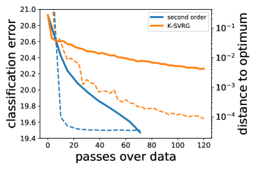
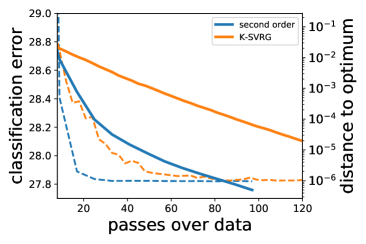
Figure 1: Training loss and test error as as function of the number of passes on the data for our algorithm vs. K-SVRG. on the (left) Susy and (right) Higgs data sets.

To find reasonable $\lambda$ for supervised learning applications, we cross-validated $\lambda$ finding the minimum test error at $\lambda=10^{-10}$ for Susy and $\lambda=10^{-9}$ for Higgs (see Figs. 3 and 2 in Appendix F) for such values our algorithm and the competitor achieve an error of 19.5% on the test set for Susy, comparable to the state of the art (19.6% [29]) and analogously for Higgs (see Appendix F). We then used such $\lambda$’s as regularization parameters and compared our algorithm with a well known accelerated stochastic gradient technique Katyusha SVRG (K-SVRG) [4], tailored to our problem using mini batches. In Fig. 1 we show the convergence of the training loss and classification error with respect to the number of passes on the data, of our algorithm compared to K-SVRG. It is possible to note our algorithm is order of magnitude faster in achieving convergence, validating empirically the fact that the proposed algorithm scales as $O(n\mathsf{df}_{\lambda})$ in learning settings, while accelerated first order methods go as $O((n+\sqrt{nL/\lambda})\mathsf{df}_{\lambda})$. Moreover, as mentioned in the introduction, this highlights the fact that precise optimization is necessary to achieve a good performance in terms of test error. Finally, note that since a pass on the data is much more expensive for K-SVRG than for our second order method (see Appendix F for details), the difference in computing time between the second order scheme and K-SVRG is even more in favour of our second order method (see Figs. 5 and 4 in Appendix F).

Acknowledgments

We acknowledge support from the European Research Council (grant SEQUOIA 724063).

Organization of the Appendix

• Main results on generalized self-concordant functions
  Notations, definitions and basic results concerning generalized self-concordant functions.

• Results on approximate Newton methods
  In this section, the interaction between the notion of Dikin ellipsoid, approximate Newton methods and generalized self-concordant functions is studied. The results needed in the main paper are all concentrated in Sec. B.3. In particular the results in Lemma 2 are proven in a more general form in Lemma 11.

• Proof of bounds for the globalization scheme
  In this section, we leverage the results of the previous two sections to analyze the globalization scheme.

  • Main technical lemmas
    We start by proving the result on the inclusion of Dikin ellipsoids (Lemma 3).

  • Proof of main theorems
    In particular, a general version of Thm. 1 is proven. Moreover Remark 1 is proven in Proposition 7, while the fixed scheme to choose $(q_{k})_{k\in\mathbb{N}}$ is proven in Proposition 8.

  • Proof of Thm. 1
    Finally, we prove the properties of the globalization schemes presented in Thm. 1.

• Non-parametric learning with generalized self-concordant functions
  In this section, some basic results about non-parametric learning with generalized self-concordant functions are recalled and the main results of Sec. 4 are proven.

  • General setting and assumptions, statistical result for regularized ERM.
    More details about the generalization properties of empirical risk minimization as well as the optimal rates in Thm. 2 are recalled.

  • Reducing the dimension: projecting on a subspace using Nyström sub-sampling.

  • Sub-sampling techniques.
    The basics of uniform sub-sampling and sub-sampling with approximate leverage scores are recalled.

  • Selecting the $M$ Nyström points
    Thm. 3 is proven in a more general version in Thm. 6.

  • Performing the globalization scheme to approximate $\beta_{M,\lambda}$
    A general scheme is proposed to solve the projected problem approximately using the globalization scheme.

    • Performing approximate Newton steps
      We start by describing the way of computing approximate Newton steps. A generalized version of Lemma 4 is proven in Proposition 12.

    • Applying the globalization scheme to control $\widehat{\nu}_{M,\lambda}(\beta)$
      We then completely analyse the approximating of $\beta_{M,\lambda}$ from an optimization point of view (see Proposition 13).

  • Final algorithm and results
    Finally, the proof of Thm. 4 is provided, using the results of the previous subsections.

• Algorithm
  In this section, the pseudocode for the algorithm presented in Sec. 4 and analyzed in Thm. 7 is provided.

• Experiments
  In this section, more details about the experiments are provided.

• Solving a projected problem to reduce dimension
  In this section, more details about the problem of randomized projections are provided.

  • Relating the projected to the original problem
    In particular, results to relate the ERM with the projected ERM in terms of excess risk are provided for generalized self-concordant functions.

• Relations between statistical problems and empirical problem.
  In this section, we provide results to relate excess expected risk with excess empirical risk for generalized self-concordant functions.

• Multiplicative approximations for Hermitian operators
  In this section, some general analytic results on multiplicative approximations for Hermitian operators are derived. Moreover they are used to provide a simplified proof for the results in Lemma 1. See in particular Lemmas 28 and 29 and [25], Lemma 2.

Appendix A Main results on generalized self-concordant functions

In this section, we start by introducing a few notations. We define the key notion of generalized self-concordance in Sec. A.1, and present the main results concerning generalized self-concordant functions. In Sec. A.2, we describe how generalized self-concordance behaves with respect to an expectation or to certain relaxations.

Notations

Let $\lambda\geqslant 0$ and $\mathbf{A}$ be a bounded positive semidefinite Hermitian operator on ${\mathcal{H}}$. We denote with $\mathbf{I}$ the identity operator, and

$$\|x\|_{\mathbf{A}} :=\|\mathbf{A}^{1/2}x\|,$$ (11)

$$\mathbf{A}_{\lambda} :=\mathbf{A}+\lambda\mathbf{I}.$$ (12)

Let $f$ be a twice differentiable convex function on a Hilbert space ${\mathcal{H}}$. We adopt the following notation for the Hessian of $f$:

$$\forall x\in{\mathcal{H}},\leavevmode\nobreak\ \mathbf{H}_{f}(x):=\nabla^{2}f(x)\in\mathcal{L}({\mathcal{H}}).$$

For any $\lambda>0$, we define the $\lambda$-regularization of $f$:

$$f_{\lambda}:=f+\frac{\lambda}{2}\|\cdot\|^{2}.$$

$f_{\lambda}$ is $\lambda$-strongly convex and has a unique minimizer which we denote with $x^{f,\lambda}_{\star}$. Moreover, define

$$\forall x\in{\mathcal{H}},\leavevmode\nobreak\ \mathbf{H}_{f,\lambda}(x):=\nabla^{2}f_{\lambda}(x)=\mathbf{H}_{f}(x)+\lambda\mathbf{I},\qquad\nu_{f,\lambda}(x):=\|\nabla f_{\lambda}(x)\|_{\mathbf{H}_{f,\lambda}^{-1}(x)}.$$

The quantity $\nu_{f,\lambda}(x)$ is called the Newton decrement at point $x$ and will play a significant role.

When the function $f$ is clear from the context, we will omit the subscripts with $f$ and use $\mathbf{H},\mathbf{H}_{\lambda},\nu_{\lambda}...$.

A.1 Definitions and results on generalized self-concordant functions

In this section, we introduce the main definitions and results for self-concordant functions. These results are mainly the same as in appendix B of [23].

Definition 3 (generalized self-concordant function).

Let ${\mathcal{H}}$ be a Hilbert space. Formally, a generalized self-concordant function on ${\mathcal{H}}$ is a couple $(f,\mathcal{G})$ where:

1. $\mathcal{G}$ is a bounded subset of ${\mathcal{H}}$; we will usually denote $\|\mathcal{G}\|$ or $R$ the quantity $\sup_{g\in\mathcal{G}}\|g\|<\infty$;

2. $f$ is a convex and three times differentiable mapping on ${\mathcal{H}}$ such that

   $$\forall x\in{\mathcal{H}},\leavevmode\nobreak\ \forall h,k\in{\mathcal{H}},\leavevmode\nobreak\ \nabla^{(3)}f(x)[h,k,k]\leqslant\sup_{g\in\mathcal{G}}|g\cdot h|\leavevmode\nobreak\ \nabla^{2}f(x)[k,k].$$

To make notations lighter, we will often omit $\mathcal{G}$ from the notations and simply say that $f$ stands both for the mapping and the couple $(f,\mathcal{G})$.

Definition 4 (Definitions).

Let $f$ be a generalized self-concordant function. We define the following quantities.

• $\forall h\in{\mathcal{H}},\leavevmode\nobreak\ \mathsf{t}_{f}(h):=\sup_{g\in\mathcal{G}}|h\cdot g|$;

• $\forall x\in{\mathcal{H}},\leavevmode\nobreak\ \forall\lambda>0,\leavevmode\nobreak\ \mathsf{r}_{f,\lambda}(x):=\frac{1}{\sup_{g\in\mathcal{G}}\|g\|_{\mathbf{H}^{-1}_{f,\lambda}(x)}}$;

• $\forall\mathsf{c}\geqslant 0,\leavevmode\nobreak\ \forall\lambda>0,\leavevmode\nobreak\ \mathsf{D}_{f,\lambda}(\mathsf{c}):=\left\{x\leavevmode\nobreak\ :\leavevmode\nobreak\ \nu_{f,\lambda}(x)\leqslant\mathsf{c}\mathsf{r}_{f,\lambda}(x)\right\}$.

We also define the following functions:

$$\psi(t)=\frac{e^{t}-t-1}{t^{2}},\quad\underline{\phi}(t)=\frac{1-e^{-t}}{t},\quad\overline{\phi}(t)=\frac{e^{t}-1}{t}.$$ (13)

Note that $\psi$, $\overline{\phi}$ are increasing functions and that $\underline{\phi}$ is a decreasing function. Moreover, $\frac{\overline{\phi}(t)}{\underline{\phi}(t)}=e^{t}$. Once again, if $f$ is clear, we will often omit the reference to $f$ in the quantities above, keeping only $\mathsf{t},\mathsf{r}_{\lambda},\mathsf{D}_{\lambda}...$

We condense results obtained in [23] under a slightly different form. The proofs, however, are exactly the same.

While in [23], only the regularized case is dealt with, the proof techniques are exactly the same to obtain Proposition 1. Proposition 2 is proved explicitly in Proposition 4 of [23] and Lemma 5 is proved in Proposition 5.
 Omitting the subscript $f$, we get the following results.

Proposition 1 (Bounds for the non-regularized function $f$).

Let $f$ be a generalized self-concordant function. Then the following bounds hold (we omit $f$ in the subscripts):

$$\forall x\in{\mathcal{H}},\leavevmode\nobreak\ \forall h\in{\mathcal{H}},\leavevmode\nobreak\ e^{-\mathsf{t}(h)}\mathbf{H}(x)\preceq\mathbf{H}(x+h)\preceq e^{\mathsf{t}(h)}\mathbf{H}(x),$$ (14)

$$\forall x,h\in{\mathcal{H}},\leavevmode\nobreak\ \forall\lambda>0,\leavevmode\nobreak\ \|\nabla f(x+h)-\nabla f(x)\|_{\mathbf{H}^{-1}_{\lambda}(x)}\leqslant\overline{\phi}(\mathsf{t}(h))\|h\|_{\mathbf{H}_{\lambda}(x)},$$ (15)

$$\forall x,h\in{\mathcal{H}},\leavevmode\nobreak\ \psi(-\mathsf{t}(h))\|h\|^{2}_{\mathbf{H}(x)}\leqslant f(x+h)-f(x)-\nabla f(x).h\leqslant\psi(\mathsf{t}(h))\|h\|^{2}_{\mathbf{H}(x)}.$$ (16)

We get the analoguous bounds in the regularized case.

Proposition 2 (Bounds for the regularized function $f_{\lambda}$).

Let $f$ be a generalized self-concordant function and $\lambda>0$ be a regularizer. Then the following bounds hold:

$$\forall x,h\in{\mathcal{H}},\leavevmode\nobreak\ e^{-\mathsf{t}(h)}\mathbf{H}_{\lambda}(x)\preceq\mathbf{H}_{\lambda}(x+h)\preceq e^{\mathsf{t}(h)}\mathbf{H}_{\lambda}(x),$$ (17)

$$\forall x,h\in{\mathcal{H}},\leavevmode\nobreak\ \underline{\phi}(\mathsf{t}(h))\|h\|_{\mathbf{H}_{\lambda}(x)}\leqslant\|\nabla f_{\lambda}(x+h)-\nabla f_{\lambda}(x)\|_{\mathbf{H}^{-1}_{\lambda}(x)}\leqslant\overline{\phi}(\mathsf{t}(h))\|h\|_{\mathbf{H}_{\lambda}(x)},$$ (18)

$$\forall x,h\in{\mathcal{H}},\leavevmode\nobreak\ \psi(-\mathsf{t}(h))\|h\|^{2}_{\mathbf{H}_{\lambda}(x)}\leqslant f_{\lambda}(x+h)-f_{\lambda}(x)-\nabla f_{\lambda}(x).h\leqslant\psi(\mathsf{t}(h))\|h\|^{2}_{\mathbf{H}_{\lambda}(x)}.$$ (19)

Corollary 1.

Let $f$ be a $\mathcal{G}$ generalized self-concordant function and $\lambda>0$ be a regularizer, and $x_{\lambda}^{\star}$ the unique minimizer of $f_{\lambda}$. Then the following bounds hold for any $x\in{\mathcal{H}}$:

$$\underline{\phi}(\mathsf{t}(x-x_{\lambda}^{\star}))\|x-x_{\lambda}^{\star}\|_{\mathbf{H}_{\lambda}(x)}\leqslant\underbrace{\|\nabla f_{\lambda}(x)\|_{\mathbf{H}^{-1}_{\lambda}(x)}}_{\nu_{\lambda}(x)}\leqslant\overline{\phi}(\mathsf{t}(x-x_{\lambda}^{\star}))\|x-x_{\lambda}^{\star}\|_{\mathbf{H}_{\lambda}(x)},$$ (20)

$$\psi(-\mathsf{t}(x-x_{\lambda}^{\star}))\|x-x_{\lambda}^{\star}\|^{2}_{\mathbf{H}_{\lambda}(x_{\lambda}^{\star})}\leqslant f_{\lambda}(x)-f_{\lambda}(x_{\lambda}^{\star})\leqslant\psi(\mathsf{t}(x-x_{\lambda}^{\star}))\|x-x_{\lambda}^{\star}\|^{2}_{\mathbf{H}_{\lambda}(x_{\lambda}^{\star})}.$$ (21)

Moreover, the following localization lemma holds.

Lemma 5 (localization).

Let $\lambda>0$ be fixed. If $\frac{\nu_{\lambda}(x)}{\mathsf{r}_{\lambda}(x)}<1$, then

$$\mathsf{t}(x-x_{\lambda}^{\star})\leqslant-\log\left(1-\frac{\nu_{\lambda}(x)}{\mathsf{r}_{\lambda}(x)}\right).$$ (22)

In particular, this shows:

$$\forall\mathsf{c}<1,\leavevmode\nobreak\ \forall\lambda>0,\leavevmode\nobreak\ x\in\mathsf{D}_{\lambda}(\mathsf{c})\implies\mathsf{t}(x-x_{\lambda}^{\star})\leqslant-\log(1-\mathsf{c}).$$

We now state a Lemma which shows that the difference to the optimum in function values is equivalent to the squared newton decrement in a small Dikin ellipsoid. We will use this result in the main paper.

Lemma 6 (Equivalence of norms).

Let $\lambda>0$ and $x\in\mathsf{D}_{\lambda}(\frac{1}{7})$. Then the following holds:

$$\frac{1}{4}\nu_{\lambda}(x)^{2}\leqslant f_{\lambda}(x)-f_{\lambda}(x_{\lambda}^{\star})\leqslant\nu_{\lambda}(x)^{2}.$$

Proof.Apply Lemma 5 knowing $x\in\mathsf{D}_{\lambda}(\frac{1}{7})$ to get $\mathsf{t}(x-x_{\lambda}^{\star})\leqslant\log(7/6)$. Then apply Eq. 19 and Eq. 18 to get:

$$f_{\lambda}(x)-f_{\lambda}(x_{\lambda}^{\star}) \leqslant\psi(\mathsf{t}(x-x_{\lambda}^{\star}))\|x-x_{\lambda}^{\star}\|_{\mathbf{H}_{\lambda}(x_{\lambda}^{\star})}^{2}$$

$$\leqslant e^{\mathsf{t}(x-x_{\lambda}^{\star})}\psi(\mathsf{t}(x-x_{\lambda}^{\star}))\|x-x_{\lambda}^{\star}\|_{\mathbf{H}_{\lambda}(x)}^{2}$$

$$\leqslant\frac{e^{\mathsf{t}(x-x_{\lambda}^{\star})}\psi(\mathsf{t}(x-x_{\lambda}^{\star}))}{\underline{\phi}(\mathsf{t}(x-x_{\lambda}^{\star}))^{2}}\nu_{\lambda}(x)^{2}.$$

Replacing with the bound above, we get

$$\forall\lambda>0,\leavevmode\nobreak\ \forall x\in\mathsf{D}_{\lambda}(\frac{1}{7}),\leavevmode\nobreak\ f_{\lambda}(x)-f_{\lambda}(x_{\lambda}^{\star})\leqslant\nu_{\lambda}(x)^{2}.$$

For the lower bound, proceed in exactly the same way.

A.2 Comparison between generalized self-concordant functions

The following result is straightforward.

Lemma 7 (Comparison between generalized self-concordant functions).

Let $\mathcal{G}_{1}\subset\mathcal{G}_{2}\subset{\mathcal{H}}$ be two bounded subsets. If $(f,\mathcal{G}_{1})$ is generalized self-concordant, then $(f,\mathcal{G}_{2})$ is also generalized self-concordant. Moreover,

$$\forall x\in{\mathcal{H}},\leavevmode\nobreak\ \forall\lambda>0,\leavevmode\nobreak\ \mathsf{r}_{(f,\mathcal{G}_{1}),\lambda}(x)\geqslant\mathsf{r}_{(f,\mathcal{G}_{2}),\lambda}(x).$$

In particular, we will often use the following fact. If $(f,\mathcal{G})$ is generalized self-concordant, and $\mathcal{G}$ is bounded by $R$, then $(f,B_{{\mathcal{H}}}(R))$ is also generalized self-concordant. Moreover,

$$\mathsf{r}_{(f,B_{{\mathcal{H}}}(R)),\lambda}(x)=\frac{\sqrt{\lambda+\lambda_{\min}(\mathbf{H}_{f}(x))}}{R}\geqslant\frac{\sqrt{\lambda}}{R}.$$

We now state a result which shows that, given a family of generalized self-concordant functions, the expectancy of that family is also generalized self-concordant. This can be seen as a reformulation of Proposition 2 of [23].

Proposition 3 (Expectation).

Let $\mathcal{Z}$ be a polish space equipped with its Borel sigma-algebra, and ${\mathcal{H}}$ be a Hilbert space. Let $((f_{z},\mathcal{G}_{z}))_{z\in\mathcal{Z}}$ be a family of generalized self-concordant functions such that the mapping $(z,x)\mapsto f_{z}(x)$ is measurable.

Assume we are given a random variable $Z$ on $\mathcal{Z}$, whose support we denote with $\operatorname{supp}(Z)$, such that

• the random variables $\|f_{Z}(0)\|,\|\nabla f_{Z}(0)\|,\operatorname{Tr}(\nabla^{2}f_{Z}(0))$ are are bounded;

• $\mathcal{G}:=\bigcup_{z\in\operatorname{supp}(Z)}\mathcal{G}_{z}$ is a bounded subset of ${\mathcal{H}}$.

Then the mapping $f:x\in{\mathcal{H}}\mapsto\mathbb{E}\left[f_{Z}(x)\right]$ is well defined, $(f,\mathcal{G})$ is generalized self-concordant, and we can differentiate under the expectation.

Corollary 2.

Let $n\in\mathbb{N}$ and $(f_{i},\mathcal{G}_{i})_{1\leqslant i\leqslant n}$ be a family of generalized self-concordant functions. Define

$$f(x)=\frac{1}{n}\sum_{i=1}^{n}{f_{i}(x)},\leavevmode\nobreak\ \mathcal{G}=\bigcup_{i=1}^{n}{\mathcal{G}_{i}}.$$

Then $(f,\mathcal{G})$ is generalized self-concordant.

Appendix B Results on approximate Newton methods

In this section, we assume we are given a generalized self-concordant function $f$ in the sense of Appendix A. As $f$ will be fixed throughout this part, we will omit it from the notations. Recall the definitions from Definition 4:

$$\nu_{\lambda}(x):=\|\nabla f_{\lambda}(x)\|_{\mathbf{H}_{\lambda}^{-1}(x)},\leavevmode\nobreak\ \frac{1}{\mathsf{r}_{\lambda}(x)}:=\sup_{g\in\mathcal{G}}{\|g\|_{\mathbf{H}_{\lambda}^{-1}(x)}},\leavevmode\nobreak\ \mathsf{D}_{\lambda}(\mathsf{c}):=\left\{x\leavevmode\nobreak\ :\leavevmode\nobreak\ \frac{\nu_{\lambda}(x)}{\mathsf{r}_{\lambda}(x)}\leqslant\mathsf{c}\right\}.$$

Define the following quantities:

• the true Newton step at point $x$ for the $\lambda$-regularized problem:

  $$\Delta_{\lambda}(x):=\mathbf{H}_{\lambda}^{-1}(x)\nabla f_{\lambda}(x).$$

• the renormalized Newton decrement $\widetilde{\nu}_{\lambda}(x)$:

  $$\widetilde{\nu}_{\lambda}(x):=\frac{\nu_{\lambda}(x)}{\mathsf{r}_{\lambda}(x)}.$$

Moreover, note that a direct application of Eq. 17 yields the following equation which relates the radii at different points:

$$\forall\lambda>0,\leavevmode\nobreak\ \forall x\in{\mathcal{H}},\leavevmode\nobreak\ \forall h\in{\mathcal{H}},\leavevmode\nobreak\ e^{-\mathsf{t}(h)}\mathsf{r}_{\lambda}(x)\leqslant\mathsf{r}_{\lambda}(x+h)\leqslant e^{\mathsf{t}(h)}\mathsf{r}_{\lambda}(x).$$ (23)

In this appendix, we develop a complete analysis of so-called approximate Newton methods in the case of generalized self-concordant losses. By "approximate Newton method", we mean that instead of performing the classical update $x_{t+1}=x_{t}-\Delta_{\lambda}(x_{t})$, we perform an update of the form $x_{t+1}=x_{t}-\widetilde{\Delta}_{t}$ where $\widetilde{\Delta}_{t}$ is an approximation of the real Newton step. We will characterize this approximation by measuring its distance to the real Newton step using two parameters $\rho$ and $\epsilon_{0}$:

$$\|\widetilde{\Delta}_{t}-\Delta_{\lambda}(x_{t})\|\leqslant\rho\nu_{\lambda}(x_{t})+\epsilon_{0}.$$

We start by presenting a few technical results in Sec. B.1. We continue by proving that an approximate Newton method has linear convergence guarantees in the right Dikin ellipsoid in Sec. B.2. In Sec. B.3, we adapt these results to a certain way of computing approximate Newton steps, which will be the one we use in the core of the paper. In Sec. B.4, we mention ways to reduce the computational burden of these methods by showing that since all Hessians are equivalent in Dikin ellipsoids, one can actually sketch the Hessian at one given point in that ellipsoid instead of re-sketching it at each Newton step. For the sake of simplicity, this is not mentioned in the core paper, but works very well in practice.

B.1 Main technical results

We start with a technical decomposition of the Newton decrement at point $x-\widetilde{\Delta}$ for a given $\widetilde{\Delta}\in{\mathcal{H}}$.

Lemma 8 (Technical decomposition).

Let $\lambda>0$, $x\in{\mathcal{H}}$ be fixed. Assume we perform a step of the form $x-\widetilde{\Delta}$ for a certain $\widetilde{\Delta}\in{\mathcal{H}}$. Define

$$\delta:=\|\widetilde{\Delta}-\Delta_{\lambda}(x)\|_{\mathbf{H}_{\lambda}(x)},\qquad\widetilde{\delta}:=\frac{\delta}{\mathsf{r}_{\lambda}(x)}.$$

The following holds:

$$\widetilde{\nu}_{\lambda}(x-\widetilde{\Delta}) \leqslant e^{\widetilde{\nu}_{\lambda}(x)+\widetilde{\delta}}\left[\psi(\widetilde{\nu}_{\lambda}(x)+\widetilde{\delta})(\widetilde{\nu}_{\lambda}(x)+\widetilde{\delta})^{2}+\widetilde{\delta}\right];$$ (24)

$$\nu_{\lambda}(x-\widetilde{\Delta}_{\lambda}(x)) \leqslant e^{\widetilde{\nu}_{\lambda}(x)+\widetilde{\delta}}\left[\psi(\widetilde{\nu}_{\lambda}(x)+\widetilde{\delta})(\widetilde{\nu}_{\lambda}(x)+\widetilde{\delta})(\nu_{\lambda}(x)+\delta)+\delta\right].$$ (25)

Proof.

Note that by definition, $\nabla f_{\lambda}(x)=\mathbf{H}_{\lambda}(x)\Delta_{\lambda}(x)$. Hence

$$\|\nabla f^{\lambda}(x-\widetilde{\Delta})\|_{\mathbf{H}_{\lambda}^{-1}(x)} =\|\nabla f^{\lambda}(x-\widetilde{\Delta})-\nabla f^{\lambda}(x)+\mathbf{H}_{\lambda}(x)\Delta_{\lambda}(x)\|_{\mathbf{H}_{\lambda}^{-1}(x)}$$

$$\leqslant\|\nabla f^{\lambda}(x-\widetilde{\Delta})-\nabla f^{\lambda}(x)+\mathbf{H}_{\lambda}(x)\widetilde{\Delta}\|_{\mathbf{H}_{\lambda}^{-1}(x)}$$

$$+\|\mathbf{H}_{\lambda}(x)(\Delta_{\lambda}(x)-\widetilde{\Delta})\|_{\mathbf{H}_{\lambda}^{-1}(x)}$$

$$=\|\int_{0}^{1}{[\mathbf{H}_{\lambda}(x-s\widetilde{\Delta})-\mathbf{H}_{\lambda}(x)]\widetilde{\Delta}ds}\|_{\mathbf{H}_{\lambda}^{-1}(x)}+\delta$$

$$\leqslant\int_{0}^{1}{\|\mathbf{H}_{\lambda}^{-1/2}(x)\mathbf{H}_{\lambda}(x-s\widetilde{\Delta})\mathbf{H}_{\lambda}^{-1/2}(x)-\mathbf{I}\|ds}\leavevmode\nobreak\ \|\widetilde{\Delta}\|_{\mathbf{H}_{\lambda}(x)}+\delta.$$

Now using Eq. 17, one has $\|\mathbf{H}_{\lambda}^{-1/2}(x)\mathbf{H}_{\lambda}(x-s\widetilde{\Delta})\mathbf{H}_{\lambda}^{-1/2}(x)-\mathbf{I}\|\leqslant e^{s\mathsf{t}(\widetilde{\Delta})}-1$, whose integral on $s$ is $\psi(\mathsf{t}(\widetilde{\Delta}))\mathsf{t}(\widetilde{\Delta})$ where $\psi$ is defined in Definition 4. Morever, bounding

$$\|\widetilde{\Delta}\|_{\mathbf{H}_{\lambda}(x)}\leqslant\|\widetilde{\Delta}-\Delta_{\lambda}(x)\|_{\mathbf{H}_{\lambda}(x)}+\|\Delta_{\lambda}(x)\|_{\mathbf{H}_{\lambda}(x)}=\delta+\nu_{\lambda}(x),$$

it holds

$$\|\nabla f^{\lambda}(x-\widetilde{\Delta})\|_{\mathbf{H}_{\lambda}^{-1}(x)}\leqslant\psi(\mathsf{t}(\widetilde{\Delta}))\mathsf{t}(\widetilde{\Delta})\leavevmode\nobreak\ (\nu_{\lambda}(x)+\delta)+\delta.$$

1.

Now note that using Eq. 17, it holds: $\nu_{\lambda}(x-\widetilde{\Delta})\leqslant e^{\mathsf{t}(\widetilde{\Delta})/2}\|\nabla f^{\lambda}(x-\widetilde{\Delta})\|_{\mathbf{H}_{\lambda}^{-1}(x)}$ and hence:

$$\nu_{\lambda}(x-\widetilde{\Delta})\leqslant e^{\mathsf{t}(\widetilde{\Delta})/2}\left(\psi(\mathsf{t}(\widetilde{\Delta}))\mathsf{t}(\widetilde{\Delta})\leavevmode\nobreak\ (\nu_{\lambda}(x)+\delta)+\delta\right).$$ (26)

2.

Moreover, using Eq. 23,

$$\widetilde{\nu}_{\lambda}(x-\widetilde{\Delta})\leqslant e^{\mathsf{t}(\widetilde{\Delta})}\left(\psi(\mathsf{t}(\widetilde{\Delta}))\mathsf{t}(\widetilde{\Delta})\leavevmode\nobreak\ (\widetilde{\nu}_{\lambda}(x)+\widetilde{\delta})+\widetilde{\delta}\right).$$ (27)

Noting that

$$\mathsf{t}(\widetilde{\Delta})\leqslant\frac{\|\widetilde{\Delta}\|_{\mathbf{H}_{\lambda}(x)}}{\mathsf{r}_{\lambda}(x)}\leqslant\widetilde{\nu}_{\lambda}(x)+\widetilde{\delta},$$

and bounding Eq. 26 simply by taking $e^{\mathsf{t}(\widetilde{\Delta})/2}\leqslant e^{\mathsf{t}(\widetilde{\Delta})}$, we get the two bounds in the lemma.

We now place ourselves in the case where we are given an approximation of the Newton step of the following form. Assume $\lambda$ and $x$ are fixed, and that we approximate $\Delta_{\lambda}(x)$ with $\widetilde{\Delta}$ such that there exists $\rho\geqslant 0$ and $\epsilon_{0}\geqslant 0$ such that it holds:

$$\|\widetilde{\Delta}-\Delta_{\lambda}(x)\|_{\mathbf{H}_{\lambda}(x)}\leqslant\rho\nu_{\lambda}(x)+\epsilon_{0}.$$

We define/prove the three different following regimes.

Lemma 9 (3 regimes).

Let $x\in\mathsf{D}_{\lambda}\left(\frac{1}{7}\right)$ and $\lambda>0$ be fixed. Let

$$0\leqslant\rho\leqslant\frac{1}{7},\leavevmode\nobreak\ \epsilon_{0}\geqslant 0\text{ s.t. }\tilde{\varepsilon}_{0}:=\frac{\epsilon_{0}}{\mathsf{r}_{\lambda}(x)}\leqslant\frac{1}{21}.$$

Let $\widetilde{\Delta}$ be an approximation of the Newton steps satisfying $\|\widetilde{\Delta}-\Delta_{\lambda}(x)\|_{\mathbf{H}_{\lambda}(x)}\leqslant\rho\nu_{\lambda}(x)+\epsilon_{0}$. The three following regimes appear.

• If $\widetilde{\nu}_{\lambda}(x)\geqslant\rho$ and $\widetilde{\nu}_{\lambda}(x)^{2}\geqslant\tilde{\varepsilon}_{0}$, then we are in the quadratic regime, i.e.

  $$\frac{10\widetilde{\nu}_{\lambda}(x-\widetilde{\Delta}_{\lambda}(x))}{3}\leqslant\left(\frac{10\widetilde{\nu}_{\lambda}(x)}{3}\right)^{2},\leavevmode\nobreak\ \nu_{\lambda}(x-\widetilde{\Delta}_{\lambda}(x))\leqslant\frac{10}{3}\widetilde{\nu}_{\lambda}(x)\nu_{\lambda}(x).$$

• If $\rho\geqslant\widetilde{\nu}_{\lambda}(x)$ and $\rho\widetilde{\nu}_{\lambda}(x)\geqslant\widetilde{\epsilon}_{0}$, then we are in the linear regime, i.e.

  $$\frac{10}{3}\widetilde{\nu}_{\lambda}(x-\widetilde{\Delta}_{\lambda}(x))\leqslant\left(\frac{10\rho}{3}\right)\left(\frac{10}{3}\widetilde{\nu}_{\lambda}(x)\right),\leavevmode\nobreak\ \nu_{\lambda}(x-\widetilde{\Delta}_{\lambda}(x))\leqslant\frac{10}{3}\widetilde{\nu}_{\lambda}(x)\nu_{\lambda}(x).$$

• If $\widetilde{\epsilon}_{0}\geqslant\widetilde{\nu}_{\lambda}(x)^{2},\rho\leavevmode\nobreak\ \widetilde{\nu}_{\lambda}(x)$, then the maximal precision of the approximation is reached, and it holds:

  $$\widetilde{\nu}_{\lambda}(x-\widetilde{\Delta}_{\lambda}(x))\leqslant 3\widetilde{\epsilon}_{0}\leqslant\frac{1}{7},\leavevmode\nobreak\ \nu_{\lambda}(x-\widetilde{\Delta}_{\lambda}(x))\leqslant 3\epsilon_{0}.$$

Proof.Using the previous lemma,

$$\widetilde{\nu}_{\lambda}(x-\widetilde{\Delta}_{\lambda}(x)) \leqslant e^{(1+\rho)\widetilde{\nu}_{\lambda}(x)+\widetilde{\epsilon}_{0}}\left[\psi((1+\rho)\widetilde{\nu}_{\lambda}(x)+\widetilde{\epsilon}_{0})((1+\rho)\widetilde{\nu}_{\lambda}(x)+\widetilde{\epsilon}_{0})^{2}+\rho\widetilde{\nu}_{\lambda}(x)+\widetilde{\epsilon}_{0}\right]$$

$$\leqslant\square_{1}(\widetilde{\nu}_{\lambda}(x),\rho,\widetilde{\epsilon}_{0})\leavevmode\nobreak\ \widetilde{\nu}_{\lambda}(x)^{2}+\square_{2}(\widetilde{\nu}_{\lambda}(x),\rho,\widetilde{\epsilon}_{0})\leavevmode\nobreak\ \rho\widetilde{\nu}_{\lambda}(x)+\square_{3}(\widetilde{\nu}_{\lambda}(x),\rho,\widetilde{\epsilon}_{0})\leavevmode\nobreak\ \widetilde{\epsilon}_{0},$$

and

$$\nu_{\lambda}(x-\widetilde{\Delta}_{\lambda}(x))\leqslant\square_{1}(\widetilde{\nu}_{\lambda}(x),\rho,\widetilde{\epsilon}_{0})\leavevmode\nobreak\ \widetilde{\nu}_{\lambda}(x)\nu_{\lambda}(x)+\square_{2}(\widetilde{\nu}_{\lambda}(x),\rho,\widetilde{\epsilon}_{0})\leavevmode\nobreak\ \rho\nu_{\lambda}(x)+\square_{3}(\widetilde{\nu}_{\lambda}(x),\rho,\widetilde{\epsilon}_{0})\leavevmode\nobreak\ \epsilon_{0},$$

where the following defintions are used:

$$\square_{1}(\widetilde{\nu},\rho,\widetilde{\epsilon}_{0}) :=e^{(1+\rho)\widetilde{\nu}+\widetilde{\epsilon}_{0}}\psi((1+\rho)\widetilde{\nu}+\widetilde{\epsilon}_{0})(1+\rho)^{2},$$

$$\square_{2}(\widetilde{\nu},\rho,\widetilde{\epsilon}_{0}) :=e^{(1+\rho)\widetilde{\nu}+\widetilde{\epsilon}_{0}},$$

$$\square_{3}(\widetilde{\nu},\rho,\widetilde{\epsilon}_{0}) :=e^{(1+\rho)\widetilde{\nu}+\widetilde{\epsilon}_{0}}\left[2\psi((1+\rho)\widetilde{\nu}+\widetilde{\epsilon}_{0})(1+\rho)\widetilde{\nu}+1\right].$$

Now assume $\widetilde{\epsilon}_{0}\leqslant\frac{1}{21}$, $\widetilde{\nu}_{\lambda}(x),\rho\leqslant\frac{1}{7}$. Replacing these values in the functions above bounds $\square_{1},\square_{2}$ and $\square_{3}$, and using the case distinction, we get the result.

B.2 General analysis of an approximate Newton method

The following proposition describes the behavior of an approximate newton method where $\rho$ and $\epsilon_{0}$ are fixed a priori.

Proposition 4 (General approximate Newton scheme results).

Let $\mathsf{c}\leqslant\frac{1}{7}$ be fixed and $x_{0}\in\mathsf{D}_{\lambda}(\mathsf{c})$ be a given starting point.
Let $\rho\leqslant\frac{1}{7}$ and $\epsilon_{0}$ such that $\epsilon_{0}\leqslant\frac{\mathsf{c}}{4}\leavevmode\nobreak\ \mathsf{r}_{\lambda}(x_{0})$.
Define the following approximate Newton scheme:

$$\forall t\geqslant 0,\leavevmode\nobreak\ x_{t+1}=x_{t}-\widetilde{\Delta}_{t},\leavevmode\nobreak\ \qquad\|\widetilde{\Delta}_{t}-\Delta_{\lambda}(x_{t})\|_{\mathbf{H}_{\lambda}(x_{t})}\leqslant\rho\nu_{\lambda}(x_{t})+\epsilon_{0}.$$

The following guarantees hold.

• $\forall t\geqslant 0,\leavevmode\nobreak\ x_{t}\in\mathsf{D}_{\lambda}(\mathsf{c})$.

• Let $t_{c}=\left\lfloor\log_{2}\log_{2}\frac{3}{10\rho}\right\rfloor+1$.

  $$\forall t\leqslant t_{c},\leavevmode\nobreak\ \frac{10\widetilde{\nu}_{\lambda}(x_{t})}{3}\leqslant\max\left(\frac{12\epsilon_{0}}{\mathsf{r}_{\lambda}(x_{0})},2^{-2^{t}}\right),$$

  $$\forall t\geqslant t_{c},\leavevmode\nobreak\ \frac{10\widetilde{\nu}_{\lambda}(x_{t})}{3}\leqslant\max\left(\frac{12\epsilon_{0}}{\mathsf{r}_{\lambda}(x_{0})},\left(\frac{10\rho}{3}\right)^{t-t_{c}+1}\right).$$

• We can bound the relative decrease for both the Newton decrement and the renormalized Newton decrement:

  $$\forall t\leqslant t_{c},\leavevmode\nobreak\ \nu_{\lambda}(x_{t})\leqslant\max\left(3\epsilon_{0},\left(\frac{1}{2}\right)^{2^{t}-1}\nu_{\lambda}(x_{0})\right),$$

  $$\widetilde{\nu}_{\lambda}(x_{t})\leqslant\max\left(\frac{18\epsilon_{0}}{5\mathsf{r}_{\lambda}(x_{0})},\left(\frac{1}{2}\right)^{2^{t}-1}\widetilde{\nu}_{\lambda}(x_{0})\right).$$

  $$\forall t\geqslant t_{c},\leavevmode\nobreak\ \nu_{\lambda}(x_{t})\leqslant\max\left(3\epsilon_{0},\left(\frac{10\rho}{3}\right)^{t-t_{c}+1}\nu_{\lambda}(x_{0})\right),$$

  $$\widetilde{\nu}_{\lambda}(x_{t})\leqslant\max\left(\frac{18\epsilon_{0}}{5\mathsf{r}_{\lambda}(x_{0})},\left(\frac{10\rho}{3}\right)^{t-t_{c}+1}\widetilde{\nu}_{\lambda}(x_{0})\right).$$

Proof.Start by noting, using Eq. 23,

$$\forall x\in\mathsf{D}_{\lambda}\left(\frac{1}{7}\right),\leavevmode\nobreak\ \varepsilon\leqslant\frac{\mathsf{r}_{\lambda}(x)}{21},\leavevmode\nobreak\ \frac{6}{7}\mathsf{r}_{\lambda}(x_{0})\leqslant\mathsf{r}_{\lambda}(x)\leqslant\frac{7}{6}\mathsf{r}_{\lambda}(x_{0}).$$ (28)

In particular, this holds for any $x\in\mathsf{D}_{\lambda}(\mathsf{c}),\leavevmode\nobreak\ \mathsf{c}\leqslant\frac{1}{7}$. Thus,

$$\forall\mathsf{c}\leqslant\frac{1}{7},\leavevmode\nobreak\ \forall x_{0}\in\mathsf{D}_{\lambda}(\mathsf{c}),\leavevmode\nobreak\ \frac{\epsilon_{0}}{\mathsf{r}_{\lambda}(x_{0})}\leqslant\frac{\mathsf{c}}{4}\implies\forall x\in\mathsf{D}_{\lambda}(\mathsf{c}),\leavevmode\nobreak\ \frac{\epsilon_{0}}{\mathsf{r}_{\lambda}(x)}\leqslant\frac{\mathsf{c}}{3}.$$

1.

Proving the first point is simple by induction. Indeed, assume $\widetilde{\nu}_{\lambda}(x_{t})\leqslant\mathsf{c}$. We can apply Lemma 9 since the conditions on $\varepsilon$ and $\rho$ guarantee that the conditions of this lemma are satisfied.

If we are in either the linear or quadratic regime, the fact that $\frac{10\rho}{3},\frac{10\widetilde{\nu}_{\lambda}(x_{t})}{3}\leqslant\frac{10}{21}$ show that $\widetilde{\nu}_{\lambda}(x_{t+1})\leqslant\frac{10}{21}\widetilde{\nu}_{\lambda}(x_{t})\leqslant\mathsf{c}$.

If we are in the last case, $\widetilde{\nu}_{\lambda}(x_{t+1})\leqslant\frac{3\epsilon_{0}}{\mathsf{r}_{\lambda}(x_{t})}\leqslant\mathsf{c}$.

2.

Let us prove the second bullet point by induction. Start by assuming the property holds at $t$. By the previous point, the hypothesis of Lemma 9 are satisfied at $x_{t}$ with $\rho$ and $\varepsilon$. Assume we are in the limiting case; we easily show that in this case,

$$\frac{10\widetilde{\nu}_{\lambda}(x_{t+1})}{3}\leqslant\frac{10}{3}\leavevmode\nobreak\ 3\frac{\epsilon_{0}}{\mathsf{r}_{\lambda}(x_{t})}\leqslant\frac{35\epsilon_{0}}{3\mathsf{r}_{\lambda}(x_{0})}.$$

Here, the last inequality comes from Eq. 28. If we are not in the limiting case, let us distinguish between the two following cases.

If $t\leqslant t_{c}-1$,

$$\frac{10\widetilde{\nu}_{\lambda}(x_{t+1})}{3} \leqslant\frac{10\widetilde{\nu}_{\lambda}(x_{t})}{3}\max\left(\frac{10\widetilde{\nu}_{\lambda}(x_{t})}{3},\frac{10\rho}{3}\right)$$

$$\leqslant\max\left(\frac{35\epsilon_{0}}{3\mathsf{r}_{\lambda}(x_{0})},\frac{10\widetilde{\nu}_{\lambda}(x_{t})}{3}\max\left(\left(\frac{1}{2}\right)^{2^{t}},\frac{10\rho}{3}\right)\right),$$

where the last inequality comes from using the induction hypothesis and the fact that $\frac{10\widetilde{\nu}_{\lambda}(x_{t})}{3}\leqslant 1$. Using once again the induction hypotheses and the fact that $t\leqslant\left\lfloor\log_{2}\log_{2}\frac{3}{10\rho}\right\rfloor$ which implies $\frac{10\rho}{3}\leqslant\left(\frac{1}{2}\right)^{2^{t}}$, we finally get

$$\frac{10\widetilde{\nu}_{\lambda}(x_{t+1})}{3}\leqslant\max\left(\frac{35\epsilon_{0}}{3\mathsf{r}_{\lambda}(x_{0})},\left(\frac{1}{2}\right)^{2^{t+1}}\right).$$

The fact that the second property holds for $t=t_{c}$ is trivial Now consider the case where $t\geqslant t_{c}$. Using the same technique as before but noting that in this case

$$\frac{10\widetilde{\nu}_{\lambda}(x_{t})}{3}\leqslant\max\left(\frac{35\epsilon_{0}}{3\mathsf{r}_{\lambda}(x_{0})},\left(\frac{10\rho}{3}\right)^{t-t_{c}+1}\right)\leqslant\max\left(\frac{35\epsilon_{0}}{3\mathsf{r}_{\lambda}(x_{0})},\frac{10\rho}{3}\right),$$

We easily use Lemma 9 to reach the desired conclusion.

3.

Let $t<t_{c}$. Then using Lemma 9:

$$\forall s\leqslant t,\leavevmode\nobreak\ \nu_{\lambda}(x_{s+1})\leqslant\max\left(3\epsilon_{0},\max(\frac{10\rho}{3},\frac{10\widetilde{\nu}_{\lambda}(x_{s})}{3})\nu_{\lambda}(x_{s})\right).$$

Using the fact that for any $s\leqslant t$, $\frac{10\widetilde{\nu}_{\lambda}(x_{s})}{3}\leqslant\max(\frac{35\epsilon_{0}}{3\mathsf{r}_{\lambda}(x_{0})},\left(\frac{1}{2}\right)^{2^{s}})$:

$$\forall s\leqslant t,\leavevmode\nobreak\ \nu_{\lambda}(x_{s+1})\leqslant\max\left(3\epsilon_{0},\frac{35\epsilon_{0}}{3}\frac{\nu_{\lambda}(x_{s})}{\mathsf{r}_{\lambda}(x_{0})},\max(\frac{10\rho}{3},\left(\frac{1}{2}\right)^{2^{s}})\nu_{\lambda}(x_{s})\right).$$

Now using the fact that for any $s\leqslant t,\leavevmode\nobreak\ \widetilde{\nu}_{\lambda}(x_{s})\leqslant\frac{1}{7}$, we see that $\frac{\nu_{\lambda}(x_{s})}{\mathsf{r}_{\lambda}(x_{0})}\leqslant\frac{7}{6}\widetilde{\nu}_{\lambda}(x_{s})\leqslant\frac{1}{6}$ and hence $\frac{35\epsilon_{0}}{3}\frac{\nu_{\lambda}(x_{s})}{\mathsf{r}_{\lambda}(x_{0})}\leqslant 3\epsilon_{0}$. Moreover, since $s\leqslant t<t_{c}$, $\max(\frac{10\rho}{3},\left(\frac{1}{2}\right)^{2^{s}})=\left(\frac{1}{2}\right)^{2^{s}}$. Thus:

$$\forall s\leqslant t,\leavevmode\nobreak\ \nu_{\lambda}(x_{s+1})\leqslant\max\left(3\epsilon_{0},\left(\frac{1}{2}\right)^{2^{s}}\nu_{\lambda}(x_{s})\right).$$

Combining these results yields:

$$\nu_{\lambda}(x_{t+1})\leqslant\max\left(3\epsilon_{0},\left(\frac{1}{2}\right)^{2^{t+1}-1}\nu_{\lambda}(x_{0})\right).$$

This shows the first equation, that is:

$$\forall t\leqslant t_{c},\leavevmode\nobreak\ \nu_{\lambda}(x_{t})\leqslant\max\left(3\epsilon_{0},\left(\frac{1}{2}\right)^{2^{t}-1}\nu_{\lambda}(x_{0})\right).$$

The case for $t\geqslant t_{c}$ is completely analogous. We can also reproduce the same proof to get the same bounds for $\widetilde{\nu}$, since the bounds in Lemma 9 are the same for both.

B.3 Main results in the paper

In the main paper, we mention two types of Newton method. First, we present a result of convergence on the full Newton method:

Lemma 10 (Quadratic convergence of the full Newton method).

Let $\mathsf{c}\leqslant\frac{1}{7}$ and $x_{0}\in\mathsf{D}_{\lambda}(\mathsf{c})$. Define

$$x_{t+1}=x_{t}-\Delta_{\lambda}(x_{t}).$$

Then this scheme converges quadratically, i.e.:

$$\forall t\in\mathbb{N},\leavevmode\nobreak\ \frac{\nu_{\lambda}(x_{t})}{\nu_{\lambda}(x_{0})},\frac{\widetilde{\nu}_{\lambda}(x_{t})}{\widetilde{\nu}_{\lambda}(x_{0})}\leqslant 2^{-(2^{t}-1)}.$$

Thus :

• $\forall t\in\mathbb{N},\leavevmode\nobreak\ x_{t}\in\mathsf{D}_{\lambda}(\mathsf{c})$.

• For any $\tilde{\mathsf{c}}\leqslant\mathsf{c}$ then $\forall t\geqslant\left\lceil\log_{2}\left(1+\log_{2}\frac{\mathsf{c}}{\tilde{\mathsf{c}}}\right)\right\rceil,\leavevmode\nobreak\ x_{t}\in\mathsf{D}_{\lambda}(\tilde{\mathsf{c}})$.

• For any $\varepsilon>0$, $\forall t\geqslant\left\lceil\log_{2}\left(1+\log_{2}\frac{\nu_{\lambda}(x_{0})}{\sqrt{\varepsilon}}\right)\right\rceil,\leavevmode\nobreak\ \nu_{\lambda}(x_{t})\leqslant\sqrt{\varepsilon},\leavevmode\nobreak\ f_{\lambda}(x)-f_{\lambda}(x_{\lambda}^{\star})\leqslant\varepsilon$.

• If we perform the Newton method and return the first $x_{t}$ such that $\nu_{\lambda}(x_{t})\leqslant\sqrt{\varepsilon}$, then the number of Newton steps computations is at most $1+\left\lceil\log_{2}\left(1+\log_{2}\frac{\nu_{\lambda}(x_{0})}{\sqrt{\varepsilon}}\right)\right\rceil$.

Proof.

A full Newton method is an approximate Newton method where $\rho,\epsilon_{0}=0$. Thus apply Proposition 4; note that in this case $t_{c}=+\infty$. The last point shows that if $\mathsf{c}\leqslant\frac{1}{7}$, and if we perform the Newton method with a full Newton step, then

$$\forall t\geqslant 0,\leavevmode\nobreak\ \widetilde{\nu}_{\lambda}(x_{t})\leqslant 2^{-(2^{t}-1)}\nu_{\lambda}(x_{0}),\leavevmode\nobreak\ \widetilde{\nu}_{\lambda}(x_{t})\leqslant 2^{-(2^{t}-1)}\nu_{\lambda}(x_{0}).$$

This shows the quadratic convergence, and the first two points directly follow. For the third point, the result for $\nu_{\lambda}(x_{t})$ directly follows from the previous equation, and the one on function values is a direct consequence of Lemma 6 and the fact that $x_{t}\in\mathsf{D}_{\lambda}(1/7)$.

For the last point, note that $\nu_{t}(x_{t})=\nabla f_{\lambda}(x_{t})\cdot\Delta_{\lambda}(x_{t})$ is accessible. Moreover, the bound on $t$ is given in the point before, and since one has to compute $\Delta_{\lambda}(x_{s})$ for $0\leqslant s\leqslant t$, there are at most $t+1$ computations.

In the main paper, we compute approximate Newton steps by considering methods which naturally yield only a relative error $\rho$ and no absolute error $\epsilon_{0}$. Indeed, we take the following notation.

Approximate solutions to linear problems.

Let $\mathbf{A}$ be a positive definite Hermitian operator on ${\mathcal{H}}$, $b$ in ${\mathcal{H}}$, and a wanted relative precision $\rho$.

We say that $x$ is a $\rho$-relative approximation to the linear problem $\mathbf{A}x=b$ and write $x\in\operatorname{LinApprox}(\mathbf{A},b,\rho)$ if the following holds:

$$\|\mathbf{A}^{-1}b-x\|_{\mathbf{A}}\leqslant\rho\|b\|_{\mathbf{A}^{-1}}=\rho\|\mathbf{A}^{-1}b\|_{\mathbf{A}}.$$

Note that if $x\in\operatorname{LinApprox}(\mathbf{A},b,\rho)$ for $\rho<1$, then

$$(1-\rho)\|b\|_{\mathbf{A}^{-1}}\leqslant x\cdot b\leqslant(1+\rho)\|b\|_{\mathbf{A}^{-1}}.$$

The following lemma shows that if, instead of computing the exact Newton step, we compute a relative approximation of the Newton step belonging to $\operatorname{LinApprox}(\mathbf{H}_{\lambda}(x),\nabla f_{\lambda}(x),\rho)$ for a given $\rho<1$, then one has linear convergence. Moreover, we show that we can still perform a method which automatically stops.

Proposition 5 (relative approximate Newton method).

Let $\lambda>0$, $\rho\leqslant\frac{1}{7}$, $\mathsf{c}\leqslant\frac{1}{7}$ and a starting point $x_{0}\in\mathsf{D}_{\lambda}(\mathsf{c})$. Assume we perform the following Newton scheme:

$$\forall t\geqslant 0,\leavevmode\nobreak\ x_{t+1}=x_{t}-\widetilde{\Delta}_{t},\leavevmode\nobreak\ \qquad\widetilde{\Delta}_{t}\in\operatorname{LinApprox}(\mathbf{H}_{\lambda}(x_{t}),\nabla f_{\lambda}(x_{t}),\rho).$$

Then the scheme converges linearly, i.e.

$$\forall t\in\mathbb{N},\leavevmode\nobreak\ \frac{\nu_{\lambda}(x_{t})}{\nu_{\lambda}(x_{0})},\frac{\widetilde{\nu}_{\lambda}(x_{t})}{\widetilde{\nu}_{\lambda}(x_{0})}\leqslant 2^{-t}.$$

Thus,

• $\forall t\in\mathbb{N},\leavevmode\nobreak\ x_{t}\in\mathsf{D}_{\lambda}(\mathsf{c})$.

• For any $\tilde{\mathsf{c}}\leqslant\mathsf{c}$ then $\forall t\geqslant\left\lceil\log_{2}\frac{\mathsf{c}}{\tilde{\mathsf{c}}}\right\rceil,\leavevmode\nobreak\ x_{t}\in\mathsf{D}_{\lambda}(\tilde{\mathsf{c}})$.

• For any $\varepsilon>0$, $\forall t\geqslant\left\lceil\log_{2}\frac{\nu_{\lambda}(x_{0})}{\sqrt{\varepsilon}}\right\rceil,\leavevmode\nobreak\ \nu_{\lambda}(x_{t})\leqslant\sqrt{\varepsilon},\leavevmode\nobreak\ f_{\lambda}(x)-f_{\lambda}(x_{\lambda}^{\star})\leqslant\varepsilon$

• If the method is performed and returns the first $x_{t}$ such that $x_{t}\cdot\widetilde{\Delta}_{t}\leqslant\frac{6}{7}\varepsilon$, then at most $2+\left\lfloor\log_{2}\left(\sqrt{\frac{4}{3}}\frac{\nu_{\lambda}(x_{0})}{\sqrt{\varepsilon}}\right)\right\rfloor$ approximate Newton steps computations have been performed, and $\nu_{\lambda}(x_{t})\leqslant\sqrt{\varepsilon},\leavevmode\nobreak\ f_{\lambda}(x)-f_{\lambda}(x_{\lambda}^{\star})\leqslant\varepsilon$.

Proof.Apply Proposition 4 with $\epsilon_{0}=0$ and $\rho=\frac{1}{7}$, since if $\rho\leqslant\frac{1}{7}$, then a fortiori the approximation satisfies the condition for $\rho=\frac{1}{7}$. The last point clearly states that

$$\forall t\in\mathbb{N},\leavevmode\nobreak\ \frac{\nu_{\lambda}(x_{t})}{\nu_{\lambda}(x_{0})},\frac{\widetilde{\nu}_{\lambda}(x_{t})}{\widetilde{\nu}_{\lambda}(x_{0})}\leqslant\left(\frac{10}{21}\right)^{t}\leqslant 2^{-t}.$$

From this, using Lemma 6 for the third point, the first three points are easily proven.
 For the last point, note that since $\widetilde{\Delta}_{t}\in\operatorname{LinApprox}(\mathbf{H}_{\lambda}(x_{t}),\nabla f_{\lambda}(x_{t}),\rho)$, the following holds: $\nabla f_{\lambda}(x_{t})\cdot\widetilde{\Delta}_{t}=\nu_{\lambda}(x_{t})^{2}+\nabla f_{\lambda}(x_{t})\cdot\left(\widetilde{\Delta}_{t}-\mathbf{H}_{\lambda}^{-1}(x_{t})\nabla f_{\lambda}(x_{t})\right)$. Now bound

$$|\nabla f_{\lambda}(x_{t})\cdot\left(\widetilde{\Delta}_{t}-\mathbf{H}_{\lambda}^{-1}(x_{t})\nabla f_{\lambda}(x_{t})\right)|\leqslant\nu_{\lambda}(x_{t})\leavevmode\nobreak\ \|\widetilde{\Delta}_{t}-\mathbf{H}_{\lambda}^{-1}(x_{t})\nabla f_{\lambda}(x_{t})\|_{\mathbf{H}_{\lambda}(x_{t})}\leqslant\rho\nu_{\lambda}(x_{t})^{2}.$$

Thus:

$$(1-\rho)\nu_{\lambda}(x_{t})^{2}\leqslant\nabla f_{\lambda}(x_{t})\cdot\widetilde{\Delta}_{t}\leqslant(1+\rho)\nu_{\lambda}(x_{t})^{2}.$$

Since $\rho=\frac{1}{7}$, we see that if $\nabla f_{\lambda}(x_{t})\cdot\widetilde{\Delta}_{t}\leqslant\frac{6}{7}\varepsilon$, then $\nu_{\lambda}(x_{t})^{2}\leqslant\varepsilon$. Moreover, since we stop at the first $t$ where $\nabla f_{\lambda}(x_{t})\cdot\widetilde{\Delta}_{t}\leqslant\frac{6}{7}\varepsilon$, then if $t$ denotes the time at which we stop,

$$\frac{6}{7}\varepsilon<\nabla f_{\lambda}(x_{t-1})\cdot\widetilde{\Delta}_{t-1}\leqslant\frac{8}{7}\nu_{\lambda}(x_{t-1})^{2}\implies\nu_{\lambda}(x_{t-1})^{2}\geqslant\frac{3}{4}\varepsilon.$$

Since $\nu_{\lambda}(x_{t-1})^{2}\leqslant 2^{-2(t-1)}\nu_{\lambda}(x_{0})^{2}$, this implies in turn that $t-1\leqslant\log_{2}\left(\sqrt{\frac{4}{3}}\frac{\nu_{\lambda}(x_{0})}{\sqrt{\varepsilon}}\right)$. Thus, necessarily, $t\leqslant 1+\left\lfloor\log_{2}\left(\sqrt{\frac{4}{3}}\frac{\nu_{\lambda}(x_{0})}{\sqrt{\varepsilon}}\right)\right\rfloor$, and since we compute approximate Newton steps for $s=0,...,t$, we finally have that the number of approximate Newton steps is bounded by

$$2+\left\lfloor\log_{2}\left(\sqrt{\frac{4}{3}}\frac{\nu_{\lambda}(x_{0})}{\sqrt{\varepsilon}}\right)\right\rfloor.$$

Last but not least, we summarize all these theorem in the following simple result.

Lemma 11.

Let $\lambda>0,\mathsf{c}\leqslant 1/7$, let $f_{\lambda}$ be generalized self-concordant and $x\in\mathsf{D}_{\lambda}(\mathsf{c})$. It holds: $\frac{1}{4}\nu_{\lambda}(x)^{2}\leqslant f_{\lambda}(x)-f_{\lambda}(x_{\lambda}^{\star})\leqslant\nu_{\lambda}(x)^{2}$. Moreover, the full Newton method starting from $x_{0}$ has quadratic convergence, i.e. if $x_{t}$ is obtained via $t\in\mathbb{N}$ steps of the Newton method Eq. 2, then $\nu_{\lambda}(x_{t})\leqslant 2^{-(2^{t}-1)}\nu_{\lambda}(x_{0}).$ Finally, the approximate Newton method starting from $x_{0}$ has linear convergence, i.e. if $x_{t}$ is obtained via $t\in\mathbb{N}$ steps of Eq. 3, with $\widetilde{\Delta}_{t}\in\operatorname{LinApprox}(\mathbf{H}_{\lambda}(x_{t}),\nabla f_{\lambda}(x_{t}),\rho)$ and $\rho\leqslant 1/7$, then $\nu_{\lambda}(x_{t})\leqslant 2^{-t}\nu_{\lambda}(x_{0}).$

Proof.The three points are obtained in the following lemmas, assuming $x\in\mathsf{D}_{\lambda}(1/7)$.

• For $\frac{1}{4}\nu_{\lambda}(x)^{2}\leqslant f_{\lambda}(x)-f_{\lambda}(x_{\lambda}^{\star})\leqslant\nu_{\lambda}(x)^{2}$, see Lemma 6 in Sec. A.1.

• The convergence rate of the full Newton method starting in $\mathsf{D}_{\lambda}(1/7)$ is obtained in Lemma 10.

• The convergence rate of the approximate Newton method starting in $\mathsf{D}_{\lambda}(1/7)$ is obtained in Proposition 5.

B.4 Sketching the Hessian only once in each Dikin ellispoid

In this section, we provide a lemma which shows in essence that if we are in a small Dikin ellipsoid, then we can keep the Hessian of the starting point and compute approximations of $\mathbf{H}_{\lambda}^{-1}(x_{0})\nabla f_{\lambda}(x_{t})$; they will be good approximations to $\mathbf{H}_{\lambda}^{-1}(x_{t})\nabla f_{\lambda}(x_{t})$ as well.

Lemma 12.

Let $\mathsf{c}<1$ and $x_{0}\in\mathsf{D}_{\lambda}(\mathsf{c})$ be fixed.

Let $\widetilde{\mathbf{H}}$ be an approximation of the Hessian at $x_{0}$, approximation wich we quantify with

$$t:=\|\mathbf{H}^{-1/2}_{\lambda}(x_{0})\left(\mathbf{H}_{\lambda}(x_{0})-\widetilde{\mathbf{H}}\right)\mathbf{H}^{-1/2}_{\lambda}(x_{0})\|.$$

Assume

$$1+t<2(1-\mathsf{c})^{2}.$$

Let $b\in{\mathcal{H}}$. If $\widetilde{\Delta}\in\operatorname{LinApprox}(\widetilde{\mathbf{H}}_{\lambda},b,\tilde{\rho})$, then

$$\forall x\in\mathsf{D}_{\lambda}(\mathsf{c}),\leavevmode\nobreak\ \widetilde{\Delta}\in\operatorname{LinApprox}(\mathbf{H}_{\lambda}(x),b,\rho),\leavevmode\nobreak\ \rho=\frac{(\tilde{\rho}-1)(1-\mathsf{c})^{2}+(1+t)}{2(1-\mathsf{c})^{2}-(1+t)}.$$

In particular, if $\mathsf{c}\leqslant\frac{1}{30}$, $x_{0}\in\mathsf{D}_{\lambda}(\mathsf{c})$,

$$\forall x\in\mathsf{D}_{\lambda}(\mathsf{c}),\leavevmode\nobreak\ \forall b\in{\mathcal{H}},\leavevmode\nobreak\ \widetilde{\Delta}\in\operatorname{LinApprox}(\mathbf{H}_{\lambda}(x_{0}),b,\frac{1}{20})\implies\widetilde{\Delta}\in\operatorname{LinApprox}(\mathbf{H}_{\lambda}(x),b,\frac{1}{7}).$$

Proof.First, start with a general theoretical result.

1.

Let $\mathbf{A}$ and $\mathbf{B}$ be two positive semi-definite hermitian operators. Let $\lambda>0$, $b\in{\mathcal{H}}$ and $\widetilde{\Delta}\in\operatorname{LinApprox}(\mathbf{B}_{\lambda},b,\tilde{\rho})$. Decompose

$$\|\mathbf{A}_{\lambda}^{-1}b-\widetilde{\Delta}\|_{\mathbf{A}_{\lambda}} \leqslant\|\mathbf{A}_{\lambda}^{-1}b-\mathbf{B}_{\lambda}^{-1}b\|_{\mathbf{A}_{\lambda}}+\|\mathbf{B}_{\lambda}^{-1}b-\widetilde{\Delta}\|_{\mathbf{A}_{\lambda}}$$

$$\leqslant\|\mathbf{A}_{\lambda}^{1/2}(\mathbf{A}_{\lambda}^{-1}-\mathbf{B}_{\lambda}^{-1})\mathbf{A}_{\lambda}^{1/2}\|\leavevmode\nobreak\ \|b\|_{\mathbf{A}_{\lambda}^{-1}}+\|\mathbf{A}_{\lambda}^{1/2}\mathbf{B}_{\lambda}^{-1/2}\|\leavevmode\nobreak\ \|\mathbf{B}_{\lambda}^{-1}b-\widetilde{\Delta}\|_{\mathbf{B}_{\lambda}}.$$

Now using the fact that $\mathbf{A}_{\lambda}^{-1}-\mathbf{B}_{\lambda}^{-1}=\mathbf{B}_{\lambda}^{-1}(\mathbf{B}-\mathbf{A})\mathbf{A}_{\lambda}^{-1}$,

$$\|\mathbf{A}_{\lambda}^{1/2}(\mathbf{A}_{\lambda}^{-1}-\mathbf{B}_{\lambda}^{-1})\mathbf{A}_{\lambda}^{1/2}\| \leqslant\|\mathbf{A}_{\lambda}^{-1/2}(\mathbf{B}-\mathbf{A})\mathbf{A}_{\lambda}^{-1/2}\|\leavevmode\nobreak\ \|\mathbf{A}_{\lambda}^{1/2}\mathbf{B}_{\lambda}^{-1}\mathbf{A}_{\lambda}^{1/2}\|$$

$$=\|\mathbf{A}_{\lambda}^{-1/2}(\mathbf{B}-\mathbf{A})\mathbf{A}_{\lambda}^{-1/2}\|\leavevmode\nobreak\ \|\mathbf{A}_{\lambda}^{1/2}\mathbf{B}_{\lambda}^{-1/2}\|^{2}.$$

Moreover,

$$\|\mathbf{B}_{\lambda}^{-1}b-\widetilde{\Delta}\|_{\mathbf{B}_{\lambda}}\leqslant\tilde{\rho}\|b\|_{\mathbf{B}_{\lambda}^{-1}}\leqslant\|\mathbf{A}^{1/2}\mathbf{B}^{-1/2}\|\leavevmode\nobreak\ \|b\|_{\mathbf{A}_{\lambda}^{-1}}.$$

Putting things together, and noting that from Lemma 21, $\|\mathbf{A}^{1/2}\mathbf{B}^{-1/2}\|^{2}\leqslant\frac{1}{1-\|\mathbf{A}_{\lambda}^{-1/2}(\mathbf{B}-\mathbf{A})\mathbf{A}_{\lambda}^{-1/2}\|}$ as soon as $\|\mathbf{A}_{\lambda}^{-1/2}(\mathbf{B}-\mathbf{A})\mathbf{A}_{\lambda}^{-1/2}\|<1$, it holds:

$$\widetilde{\Delta}\in\operatorname{LinApprox}(\mathbf{A}_{\lambda},b,\rho),\leavevmode\nobreak\ \rho=\frac{\tilde{\rho}+\|\mathbf{A}_{\lambda}^{-1/2}(\mathbf{B}-\mathbf{A})\mathbf{A}_{\lambda}^{-1/2}\|}{1-\|\mathbf{A}_{\lambda}^{-1/2}(\mathbf{B}-\mathbf{A})\mathbf{A}_{\lambda}^{-1/2}\|}.$$

The aim is now to apply this lemma to $\mathbf{A}=\mathbf{H}(x)$ and $\mathbf{B}=\widetilde{\mathbf{H}}$.

2.

Let $x,x_{0}\in\mathsf{D}_{\lambda}(\mathsf{c})$. Using Lemma 22, we see that

$$1+\|\mathbf{H}_{\lambda}^{-1/2}(x)(\widetilde{\mathbf{H}}-\mathbf{H}(x))\mathbf{H}_{\lambda}^{-1/2}(x)\|\leqslant(1+t)(1+\|\mathbf{H}_{\lambda}^{-1/2}(x)(\mathbf{H}(x_{0})-\mathbf{H}(x))\mathbf{H}_{\lambda}^{-1/2}(x)\|).$$

Using Eq. 17, it holds:

$$(e^{-\mathsf{t}(x-x_{0})}-1)\mathbf{I}\preceq\mathbf{H}_{\lambda}^{-1/2}(x)(\mathbf{H}(x_{0})-\mathbf{H}(x))\mathbf{H}_{\lambda}^{-1/2}(x)\preceq(e^{\mathsf{t}(x_{0}-x)}-1)\mathbf{I}.$$

Thus,

$$\|\mathbf{H}_{\lambda}^{-1/2}(x)(\mathbf{H}(x_{0})-\mathbf{H}(x))\mathbf{H}_{\lambda}^{-1/2}(x)\|\leqslant\max(1-e^{-\mathsf{t}(x-x_{0})},e^{\mathsf{t}(x-x_{0})}-1)=e^{\mathsf{t}(x-x_{0})}-1.$$

Finally, using the fact that $x_{0},x\in\mathsf{D}_{\lambda}(\mathsf{c})$ for $\mathsf{c}<1$ yields $\mathsf{t}(x-x_{0})\leqslant 2\log\frac{1}{1-\mathsf{c}}$. Hence

$$1+\|\mathbf{H}_{\lambda}^{-1/2}(x)(\mathbf{H}(x_{0})-\mathbf{H}(x))\mathbf{H}_{\lambda}^{-1/2}(x)\|\leqslant\frac{1}{(1-\mathsf{c})^{2}}.$$

Thus,

$$\|\mathbf{H}_{\lambda}^{-1/2}(x)(\widetilde{\mathbf{H}}-\mathbf{H}(x))\mathbf{H}_{\lambda}^{-1/2}(x)\|\leqslant\frac{1+t}{(1-\mathsf{c})^{2}}-1.$$

The result then follows.

Appendix C Proof of bounds for the globalization scheme

In this section, we prove that the scheme of decreasing $\mu$ towards $\lambda$ converges.

C.1 Main technical lemmas

Lemma 13 (Next $\mu$).

Let $\mu>0$, $\mathsf{c}<1$.

$$\nu_{\mu}(x)\leqslant\frac{\mathsf{c}}{3}\leavevmode\nobreak\ \frac{\sqrt{\mu}}{R}\implies\nu_{\widetilde{\mu}}(x)\leqslant\mathsf{c}\leavevmode\nobreak\ \frac{\sqrt{\widetilde{\mu}}}{R},\qquad\widetilde{\mu}:=q\leavevmode\nobreak\ \mu,\qquad q\geqslant\frac{\frac{1}{3}+\frac{R\sqrt{\mu}\|x\|_{\mathbf{H}_{\mu}^{-1}(x)}}{\mathsf{c}}}{1+\frac{R\sqrt{\mu}\|x\|_{\mathbf{H}_{\mu}^{-1}(x)}}{\mathsf{c}}}.$$

$$x\in\mathsf{D}_{\mu}\left(\frac{\mathsf{c}}{3}\right)\implies x\in\mathsf{D}_{\widetilde{\mu}}\left(\mathsf{c}\right),\qquad\widetilde{\mu}:=q\leavevmode\nobreak\ \mu,\qquad q\geqslant\frac{\frac{1}{3}+\frac{\mu\|x\|_{\mathbf{H}_{\mu}^{-1}(x)}}{\mathsf{c}\leavevmode\nobreak\ \mathsf{r}_{\mu}(x)}}{1+\frac{\mu\|x\|_{\mathbf{H}_{\mu}^{-1}(x)}}{\mathsf{c}\leavevmode\nobreak\ \mathsf{r}_{\mu}(x)}}.$$

Proof.For any $\widetilde{\mu}<\mu$, note that

$$\forall x\in{\mathcal{H}},\leavevmode\nobreak\ \|\mathbf{H}_{\widetilde{\mu}}^{-1/2}(x)\mathbf{H}_{\mu}^{1/2}(x)\|=\sqrt{\frac{\lambda_{\min}(\mathbf{H}(x))+\mu}{\lambda_{\min}(\mathbf{H}(x))+\widetilde{\mu}}}\leqslant\sqrt{\mu/\widetilde{\mu}}.$$

This shows that $\|\cdot\|_{\mathbf{H}_{\widetilde{\mu}}^{-1}(x)}\leqslant\sqrt{\frac{\mu}{\widetilde{\mu}}}\leavevmode\nobreak\ \|\cdot\|_{\mathbf{H}_{\mu}^{-1}(x)}$, and in particular that $\frac{1}{\mathsf{r}_{\widetilde{\mu}}(x)}\leqslant\sqrt{\mu/\widetilde{\mu}}\frac{1}{\mathsf{r}_{\mu}(x)}$.

Using this fact, it holds:

$$\widetilde{\nu}_{\widetilde{\mu}}(x) =\frac{\|\nabla f_{\widetilde{\mu}}(x)\|_{\mathbf{H}^{-1}_{\widetilde{\mu}}(x)}}{\mathsf{r}_{\widetilde{\mu}}(x)}$$

$$=\frac{\|\nabla f_{\mu}(x)-(\mu-\widetilde{\mu})x\|_{\mathbf{H}^{-1}_{\widetilde{\mu}}(x)}}{\mathsf{r}_{\widetilde{\mu}}(x)}$$

$$\leqslant\frac{\mu}{\widetilde{\mu}}\leavevmode\nobreak\ \frac{\|\nabla f_{\mu}(x)\|_{\mathbf{H}_{\mu}^{-1}(x)}}{\mathsf{r}_{\mu}(x)}+\left(\frac{\mu}{\widetilde{\mu}}-1\right)\frac{\|\mu x\|_{\mathbf{H}^{-1}_{\mu}(x)}}{\mathsf{r}_{\mu}(x)}.$$

Hence, if $\widetilde{\nu}_{\mu}(x)\leqslant\frac{\mathsf{c}}{3}$, a condition to obtain $\widetilde{\nu}_{\widetilde{\mu}}(x)\leqslant\mathsf{c}$ is the following:

$$\frac{\mu}{\widetilde{\mu}}\left(\frac{\mathsf{c}}{3}+t\right)\leqslant\mathsf{c}+t\Leftrightarrow\widetilde{\mu}\geqslant\mu\frac{\mathsf{c}/3+t}{\mathsf{c}+t}\qquad t=\frac{\|\mu x\|_{\mathbf{H}^{-1}_{\mu}(x)}}{\mathsf{r}_{\mu}(x)}.$$

This yields the second point of the lemma. The analysis is completely analoguous for the first.

Lemma 14 (Useful bounds for $q$).

Let $\mu>0$. Then the following hold:

$$\forall x\in{\mathcal{H}},\leavevmode\nobreak\ \frac{\mu\|x\|_{\mathbf{H}_{\mu}^{-1}(x)}}{\mathsf{r}_{\mu}(x)}\leqslant R\sqrt{\mu}\|x\|_{\mathbf{H}_{\mu}^{-1}(x)}\leqslant R\|x\|.$$

Moreover, we can bound all of these quantities using $x_{\mu}^{\star}$:

• For any $\mathsf{c}<1$, $x\in{\mathcal{H}}$, if $x\in\mathsf{D}_{\mu}(\mathsf{c}/3)$, then the following holds:

  $$\frac{\mu\|x\|_{\mathbf{H}^{-1}_{\mu}(x)}}{\mathsf{c}\leavevmode\nobreak\ \mathsf{r}_{\mu}(x)}\leqslant\frac{1}{3}\left(1+\frac{1}{1-\mathsf{c}/3}\right)+\frac{1}{1-\mathsf{c}/3}\frac{\|\mu x_{\mu}^{\star}\|_{\mathbf{H}_{\mu}^{-1}(x_{\mu}^{\star})}}{\mathsf{c}\leavevmode\nobreak\ \mathsf{r}_{\mu}(x_{\mu}^{\star})}.$$

• For any $\mathsf{c}<1$, $x\in{\mathcal{H}}$, if $\frac{R\nu_{\mu}(x)}{\sqrt{\mu}}\leqslant\frac{\mathsf{c}}{3}$, then the following holds:

  $$\frac{R\sqrt{\mu}\|x\|_{\mathbf{H}_{\mu}^{-1}(x)}}{\mathsf{c}}\leqslant\left(1+\frac{1}{1-\mathsf{c}/3}\right)\frac{1}{3}+\sqrt{\frac{1}{1-\mathsf{c}/3}}\frac{R\sqrt{\mu}\|x_{\mu}^{\star}\|_{\mathbf{H}_{\mu}^{-1}(x_{\mu}^{\star})}}{\mathsf{c}}.$$

  Likewise, it can be shown that under the same conditions:

  $$\frac{R\|x\|}{\mathsf{c}}\leqslant\frac{R\|x_{\mu}^{\star}\|}{\mathsf{c}}+\frac{1}{3}\overline{\phi}(-\log(1-\mathsf{c}/3)).$$

Proof.The first bound is obvious. Moreover, the fact that $\widetilde{\nu}_{\mu}(x)\leqslant\frac{\mathsf{c}}{3}$ implies that $\mathsf{t}(x-x_{\mu}^{\star})\leqslant\log\frac{1}{1-\mathsf{c}/3}$. Thus, we get the classical bounds on the Hessian using Eq. 14:

$$e^{-\mathsf{t}(x-x_{\mu}^{\star})}\mathbf{H}(x)\preceq\mathbf{H}(x_{\mu}^{\star})\preceq e^{\mathsf{t}(x-x_{\mu}^{\star})}\mathbf{H}(x).$$

1. Bound on $\mu\|x\|_{\mathbf{H}_{\mu}^{-1}(x)}$.

Using Eqs. 17 and 18,

$$\mu\|x\|_{\mathbf{H}^{-1}_{\mu}(x)} =\|\nabla f_{\mu}(x)-\nabla f(x)+\nabla f(x_{\mu}^{\star})-\nabla f(x_{\mu}^{\star})\|_{\mathbf{H}^{-1}_{\mu}(x)}$$

$$\leqslant\nu_{\mu}(x)+\int_{0}^{1}{\|\mathbf{H}_{\mu}(x)^{-1/2}\mathbf{H}(x_{t})(x-x_{\mu}^{\star})\|\leavevmode\nobreak\ dt}+\|\nabla f(x_{\mu}^{\star})\|_{\mathbf{H}_{\mu}(x)},\leavevmode\nobreak\ x_{t}=tx+(1-t)x_{\mu}^{\star}.$$

Now bound $\|\mathbf{H}_{\mu}(x)^{-1/2}\mathbf{H}(x_{t})(x-x_{\mu}^{\star})\|\leqslant\|\mathbf{H}_{\mu}(x)^{-1/2}\leavevmode\nobreak\ \mathbf{H}_{\mu}(x_{t})^{1/2}\|\leavevmode\nobreak\ \|x-x_{\mu}^{\star}\|_{\mathbf{H}(x_{t})}$ and use Eq. 17 and Eq. 14 to get:

$$\|\mathbf{H}_{\mu}(x)^{-1/2}\mathbf{H}(x_{t})(x-x_{\mu}^{\star})\|\leqslant e^{t\leavevmode\nobreak\ \mathsf{t}(x-x_{\mu}^{\star})}\|x-x_{\mu}^{\star}\|_{\mathbf{H}(x)}.$$

Integrating this yields:

$$\int_{0}^{1}{\|\mathbf{H}_{\mu}(x)^{-1/2}\mathbf{H}(x_{t})(x-x_{\mu}^{\star})\|\leavevmode\nobreak\ dt}\leqslant\overline{\phi}(\mathsf{t}(x-x_{\mu}^{\star}))\leavevmode\nobreak\ \|x-x_{\mu}^{\star}\|_{\mathbf{H}(x)}\leqslant e^{\mathsf{t}(x-x_{\mu}^{\star})}\leavevmode\nobreak\ \nu_{\mu}(x).$$

Where the last inequality is obtained using the bounds between gradient and hessian distance Eq. 18. Finally, using the bound on $\mathsf{t}(x-x_{\mu}^{\star})$,

$$\mu\|x\|_{\mathbf{H}_{\mu}^{-1}(x)}\leqslant\left(1+\frac{1}{1-\mathsf{c}/3}\right)\nu_{\mu}(x)+\sqrt{\frac{1}{1-\mathsf{c}/3}}\|\nabla f(x_{\mu}^{\star})\|_{\mathbf{H}_{\mu}^{-1}(x_{\mu}^{\star})}.$$

2. Bound on $R\|x\|$.

Start by decomposing

$$R\|x\|\leqslant R\|x_{\mu}^{\star}\|+R\|x-x_{\mu}^{\star}\|.$$

Now bound

$$R\|x-x_{\mu}^{\star}\|\leqslant\frac{R}{\sqrt{\mu}}\|x-x_{\mu}^{\star}\|_{\mathbf{H}_{\mu}(x)}.$$

Using Eq. 17, $\|x-x_{\mu}^{\star}\|_{\mathbf{H}_{\mu}(x)}\leqslant\overline{\phi}(-\log(1-\mathsf{c}/3))\nu_{\mu}(x).$ Hence:

$$R\|x\|\leqslant R\|x_{\mu}^{\star}\|+\overline{\phi}(-\log(1-\mathsf{c}/3))\frac{R\nu_{\mu}(x)}{\sqrt{\mu}}.$$

3. Now assume $x\in\mathsf{D}_{\mu}(\mathsf{c}/3)$.

Using the bound on $\mu\|x\|_{\mathbf{H}^{-1}_{\mu}(x)}$, and noting that

$$\frac{1}{\mathsf{r}_{\mu}(x)}\leqslant e^{\mathsf{t}(x-x_{\mu}^{\star})/2}\frac{1}{\mathsf{r}_{\mu}(x_{\mu}^{\star})},$$

it holds:

$$\frac{\mu\|x\|_{\mathbf{H}^{-1}_{\mu}(x)}}{\mathsf{c}\leavevmode\nobreak\ \mathsf{r}_{\mu}(x)}\leqslant\frac{1}{3}\left(1+\frac{1}{1-\mathsf{c}/3}\right)+\frac{1}{1-\mathsf{c}/3}\frac{\|\mu x_{\mu}^{\star}\|_{\mathbf{H}_{\mu}^{-1}(x_{\mu}^{\star})}}{\mathsf{c}\leavevmode\nobreak\ \mathsf{r}_{\mu}(x_{\mu}^{\star})}.$$

4. Now assume $\frac{R\nu_{\mu}(x)}{\sqrt{\mu}}\leqslant\frac{\mathsf{c}}{3}$.

. We know that in particular, $x\in\mathsf{D}_{\mu}(\mathsf{c}/3)$ and hence:

$$R\sqrt{\mu}\|x\|_{\mathbf{H}_{\mu}^{-1}(x)} \leqslant\left(1+\frac{1}{1-\mathsf{c}/3}\right)\frac{R\nu_{\mu}(x)}{\sqrt{\mu}}+\sqrt{\frac{1}{1-\mathsf{c}/3}}\frac{R\mu\|x_{\mu}^{\star}\|_{\mathbf{H}_{\mu}^{-1}(x_{\mu}^{\star})}}{\sqrt{\mu}}$$

$$\leqslant\left(1+\frac{1}{1-\mathsf{c}/3}\right)\frac{\mathsf{c}}{3}+\sqrt{\frac{1}{1-\mathsf{c}/3}}R\sqrt{\mu}\|x_{\mu}^{\star}\|_{\mathbf{H}_{\mu}^{-1}(x_{\mu}^{\star})}.$$

Hence

$$\frac{R\sqrt{\mu}\|x\|_{\mathbf{H}_{\mu}^{-1}(x)}}{\mathsf{c}}\leqslant\left(1+\frac{1}{1-\mathsf{c}/3}\right)\frac{1}{3}+\sqrt{\frac{1}{1-\mathsf{c}/3}}\frac{R\sqrt{\mu}\|x_{\mu}^{\star}\|_{\mathbf{H}_{\mu}^{-1}(x_{\mu}^{\star})}}{\mathsf{c}}.$$

Likewise:

$$\frac{R\|x\|}{\mathsf{c}}\leqslant\frac{R\|x_{\mu}^{\star}\|}{\mathsf{c}}+\frac{1}{3}\overline{\phi}(-\log(1-\mathsf{c}/3)).$$

We can get the following simpler bounds.

Corollary 3 (Application to $\mathsf{c}=\frac{1}{7}$).

Applying Lemma 14 to $\mathsf{c}=\frac{1}{7}$, we get the following bounds. Let $\mu>0$.

• For any $x\in{\mathcal{H}}$, if $x\in\mathsf{D}_{\mu}(\mathsf{c}/3)$, then the following holds:

  $$\frac{7\mu\|x\|_{\mathbf{H}^{-1}_{\mu}(x)}}{\mathsf{r}_{\mu}(x)}\leqslant 1+\frac{8\|\mu x_{\mu}^{\star}\|_{\mathbf{H}_{\mu}^{-1}(x_{\mu}^{\star})}}{\mathsf{r}_{\mu}(x_{\mu}^{\star})}.$$

• For any $\mathsf{c}<1$, $x\in{\mathcal{H}}$, if $\frac{R\nu_{\mu}(x)}{\sqrt{\mu}}\leqslant\frac{\mathsf{c}}{3}$, then the following hold:

  $$7R\sqrt{\mu}\|x\|_{\mathbf{H}_{\mu}^{-1}(x)}\leqslant 1+8R\sqrt{\mu}\|x_{\mu}^{\star}\|_{\mathbf{H}_{\mu}^{-1}(x_{\mu}^{\star})}.$$

  $$7R\|x\|\leqslant 7R\|x_{\mu}^{\star}\|+1.$$

C.2 Proof of main theorems

In this section, we bound the number of iterations of our scheme in different cases.

Recall the proposed globalization scheme in the paper, where $\texttt{ANM}_{\rho}(f,x,t)$ is a method performing $t$ successive $\rho$-relative approximate Newton steps of $f$ starting at $x$.

Proposed Globalization Scheme Phase I: Getting in the Dikin ellispoid of $f_{\lambda}$ Start with $x_{0}\in{\mathcal{H}},\mu_{0}>0$, $t,T\in\mathbb{N}$ and $(q_{k})_{k\in\mathbb{N}}\in(0,1]$. For $k\in\mathbb{N}$ ${}\qquad x_{k+1}\leftarrow\texttt{ANM}_{\rho}(f_{\mu_{k}},x_{k},t)$ ${}\qquad\mu_{k+1}\leftarrow q_{k+1}\mu_{k}$ Stop when $\mu_{k+1}<\lambda$ and set $x_{last}\leftarrow x_{k}$. $K\leftarrow k$ Phase II: reach a certain precision starting from inside the Dikin ellipsoid Return $\widehat{x}\leftarrow\texttt{ANM}_{\rho}(f_{\lambda},x_{last},T)$

Throughout this section, we will denote with $K$ the value of $k$ when the scheme stops, i.e. the first value of $k$ such that $\mu_{k+1}<\lambda$.

Adaptive methods

We start by presenting an adaptive way to select $\mu_{k+1}$ from $\mu_{k}$, with theoretical guarantees. The main result is the following.

Proposition 6 (Adaptive, simple version).

Assume that we perform phase I starting at $x_{0}$ such that

$$\frac{R\nu_{\mu_{0}}(x_{0})}{\sqrt{\mu_{0}}}\leqslant\frac{1}{7}.$$

Assume that at each step $k$, we compute $x_{k+1}$ using $t=2$ iterations of the $\rho$-relative approximate Newton method. Then if at each iteration, we set:

$$\mu_{k+1}=q_{k+1}\leavevmode\nobreak\ \mu_{k},\qquad q_{k+1}:=\frac{\frac{1}{3}+7R\|x_{k+1}\|}{1+7R\|x_{k+1}\|}.$$

Then the following hold:

1.

$\forall k\leqslant K+1,\leavevmode\nobreak\ \frac{R\nu_{\mu_{k}}(x_{k})}{\sqrt{\mu_{k}}}\leqslant\frac{1}{7}$ .

2.

The decreasing parameter $q_{k+1}$ is bounded above before reaching $K$:

$$\forall k\leqslant K,\leavevmode\nobreak\ q_{k+1}\leqslant\frac{\frac{4}{3}+7R\|x^{\star}_{\mu_{k}}\|}{2+7R\|x^{\star}_{\mu_{k}}\|}\leqslant\frac{\frac{4}{3}+7R\|x^{\star}_{\lambda}\|}{2+7R\|x^{\star}_{\lambda}\|}.$$

3.

$K$ is finite,

$$K\leqslant\left\lfloor\frac{\log\frac{\mu_{0}}{\lambda}}{\log\frac{2+7R\|x^{\star}_{\lambda}\|}{\frac{4}{3}+7R\|x^{\star}_{\lambda}\|}}\right\rfloor\leqslant\left\lfloor\left(3+11R\|x_{\lambda}^{\star}\|\right)\log\frac{\mu_{0}}{\lambda}\right\rfloor,$$

and $\frac{R\nu_{\lambda}(x_{K+1})}{\sqrt{\lambda}}\leqslant\frac{1}{7}$.

Proof.

Let us prove the three points one by one.

1.

This is easily proved by induction, the keys to the induction hypothesis being:

• Using the induction hypothesis, $x_{k}\in\mathsf{D}_{\mu_{k}}(\mathsf{c})$ and hence, using Proposition 5 shows that after two iterations of the approximate Newton scheme, $\frac{\nu_{\mu_{k}}(x_{k+1})}{\nu_{\mu_{k}}(x_{k})}\leqslant\frac{1}{3}$ which implies $\frac{R\nu_{\mu_{k}}(x_{k+1})}{\sqrt{\mu_{k}}}\leqslant\frac{\mathsf{c}}{3}$.

• Now using Lemma 13, we see that that since

  $$7R\|x_{k+1}\|=\frac{R\|x_{k+1}\|}{\mathsf{c}}\geqslant\frac{R\sqrt{\mu_{k}}\|x_{k+1}\|_{\mathbf{H}^{-1}_{\mu_{k}}(x_{k+1})}}{\mathsf{c}},$$

  the hypotheses to guarantee the bound for $q_{k+1}$ hold, hence

  $$\frac{R\nu_{\mu_{k+1}}(x_{k+1})}{\sqrt{\mu_{k+1}}}\leqslant\mathsf{c}.$$

2.

Using the second bullet point of Cor. 3, we see that the previous point implies

$$\forall k\leqslant K,\leavevmode\nobreak\ 7R\|x_{k+1}\|\leqslant 7R\|x^{\star}_{\mu_{k}}\|+1\implies q_{k+1}\leqslant\frac{4/3+7R\|x^{\star}_{\mu_{k}}\|}{2+7R\|x^{\star}_{\mu_{k}}\|}.$$

Now using the fact that for any $k\leqslant K$, $\mu_{k}>\lambda$, we can use the simple fact that $\|x^{\star}_{\lambda}\|\geqslant\|x^{\star}_{\mu_{k}}\|$ to get the desired bound for $q_{k+1}$.

3.

Using the previous point clearly shows the following bound:

$$\forall k\leqslant K+1,\leavevmode\nobreak\ \mu_{k}\leqslant\left(\frac{\frac{4}{3}+7R\|x^{\star}_{\lambda}\|}{2+7R\|x^{\star}_{\lambda}\|}\right)^{k}\mu_{0}.$$

As this clearly converges to $0$ when $k$ goes to infinity, $K$ is necessarily finite. Applying this for $k=K$, we see that:

$$\lambda\leqslant\mu_{K}\leqslant\left(\frac{\frac{4}{3}+7R\|x^{\star}_{\lambda}\|}{2+7R\|x^{\star}_{\lambda}\|}\right)^{K}\mu_{0}.$$

This shows that $K\leqslant\frac{\log\frac{\mu_{0}}{\lambda}}{\log\frac{2+7R\|x^{\star}_{\lambda}\|}{\frac{4}{3}+7R\|x^{\star}_{\lambda}\|}}$.

The final bound is obtained noting that

$$\frac{2+7R\|x^{\star}_{\lambda}\|}{\frac{4}{3}+7R\|x^{\star}_{\lambda}\|}=1+\frac{1}{t},\qquad t=2+\frac{21}{2}R\|x^{\star}_{\lambda}\|,$$

and using the classical bound:

$$\frac{1}{\log(1+\frac{1}{t})}\leqslant t+1.$$

Finally, the fact that $\frac{R\nu_{\lambda}(x_{K+1})}{\sqrt{\lambda}}\leqslant\mathsf{c}$ is just a consequence of the fact that $\mu_{K+1}\leqslant\lambda\leqslant\mu_{K}$ and thus that $\lambda=q\mu_{K}$ with $q\geqslant q_{K+1}$, which is shown to satisfy the condition in Lemma 13. Hence, the lemma holds not only for $\mu_{K+1}$ but also for $\lambda$.

Remark 2 ($\mu_{0}$).

In the previous proposition, we assume start at $x_{0},\mu_{0}$ such that

$$\frac{R\nu_{\mu_{0}}(x_{0})}{\sqrt{\mu_{0}}}\leqslant\frac{1}{7}.$$

A simple way to have such a pair is simply to select:

$$x_{0}=0,\leavevmode\nobreak\ \mu_{0}=7R\|\nabla f(0)\|,$$

since $\frac{R\nu_{\mu_{0}}(x_{0})}{\sqrt{\mu_{0}}}=\frac{R\|\nabla f(0)\|_{\mathbf{H}_{\mu_{0}}^{-1}(0)}}{\sqrt{\mu_{0}}}\leqslant\frac{R\|\nabla f(0)\|}{\mu_{0}}$.

Alternatively, if one can approximately compute $\|x\|_{\mathbf{H}^{-1}_{\mu}(x)}$, one can propose the following variant, whose proof is completely analogous.

Proposition 7 (Adaptive, small variant version).

Assume that we perform phase I starting at $x_{0}$ such that

$$\frac{R\nu_{\mu_{0}}(x)}{\sqrt{\mu_{0}}}\leqslant\frac{1}{7}.$$

Then if at each iteration, we set:

$$t_{k+1}=7\sqrt{\frac{7}{6}}R\sqrt{\mu_{k}}\sqrt{x_{k+1}\cdot s_{k+1}},s_{k+1}\in\operatorname{LinApprox}(\mathbf{H}_{\mu_{k}}(x_{k+1}),x_{k+1},\frac{1}{7}),$$

and

$$\mu_{k+1}=q_{k+1}\leavevmode\nobreak\ \mu_{k},\qquad q_{k+1}:=\frac{\frac{1}{3}+t_{k+1}}{1+t_{k+1}}.$$

Then the following hold:

1.

$\forall k\leqslant K,\leavevmode\nobreak\ \frac{R\nu_{\mu_{k}}(x_{k})}{\sqrt{\mu_{k}}}\leqslant\frac{1}{7}$.

2.

The decreasing parameter $q_{k+1}$ is bounded above before reaching $K$:

$$\forall k\leqslant K,\leavevmode\nobreak\ q_{k+1}\leqslant\sup_{\mu_{0}\geqslant\mu\geqslant\lambda}\frac{\frac{7}{3}+10R\sqrt{\mu}\|x^{\star}_{\mu}\|_{\mathbf{H}^{-1}_{\mu}(x^{\star}_{\mu})}}{3+10R\sqrt{\mu}\|x^{\star}_{\mu}\|_{\mathbf{H}^{-1}_{\mu}(x^{\star}_{\mu})}}\leqslant\frac{\frac{7}{3}+10R\|x_{\lambda}^{\star}\|}{3+10R\|x_{\lambda}^{\star}\|}.$$

3.

$K$ is finite,

$$K\leqslant\left(\frac{9}{2}+15\sup_{\lambda\leqslant\mu\leqslant\mu_{0}}R\sqrt{\mu}\|x^{\star}_{\mu}\|_{\mathbf{H}^{-1}_{\mu}(x^{\star}_{\mu})}\right)\log\frac{\mu_{0}}{\lambda},$$

and $\frac{R\nu_{\lambda}(x_{K+1})}{\sqrt{\lambda}}\leqslant\frac{1}{7}$.

Proof.The main thing to note is that because of the properties of $\frac{1}{7}$-approximations, if $s_{k+1}\in\operatorname{LinApprox}(\mathbf{H}_{\mu_{k}}(x_{k+1}),x_{k+1},\frac{1}{7})$,

$$(1-\frac{1}{7})\|x_{k+1}\|_{\mathbf{H}^{-1}_{\mu_{k}}(x_{k+1})}^{2}\leqslant x_{k+1}\cdot s_{k+1}\leqslant(1+\frac{1}{7})\|x_{k+1}\|_{\mathbf{H}^{-1}_{\mu_{k}}(x_{k+1})}^{2}.$$

Hence,

$$\|x_{k+1}\|_{\mathbf{H}^{-1}_{\mu_{k}}(x_{k+1})}\leqslant\sqrt{\frac{7}{6}}\sqrt{x_{k+1}\cdot s_{k+1}}\leqslant\sqrt{\frac{4}{3}}\|x_{k+1}\|_{\mathbf{H}^{-1}_{\mu_{k}}(x_{k+1})}.$$

Hence, $t_{k+1}\geqslant 7R\sqrt{\mu_{k}}\|x_{k+1}\|_{\mathbf{H}^{-1}_{\mu_{k}}(x_{k+1})}$, and we can apply Lemma 13 to get the first point.
 To get the second point, we bound $t_{k+1}$ above:

$$t_{k+1}\leqslant 7\sqrt{\frac{4}{3}}R\sqrt{\mu_{k}}\|x_{k+1}\|_{\mathbf{H}^{-1}_{\mu_{k}}(x_{k+1})}.$$

Now use Cor. 3 to find:

$$t_{k+1}\leqslant\sqrt{\frac{4}{3}}\left(1+8R\sqrt{\mu_{k}}\|x^{\star}_{\mu_{k}}\|_{\mathbf{H}^{-1}_{\mu_{k}}(x^{\star}_{\mu_{k}})}\right)\leqslant 2+10R\sqrt{\mu_{k}}\|x^{\star}_{\mu_{k}}\|_{\mathbf{H}^{-1}_{\mu_{k}}(x^{\star}_{\mu_{k}})}.$$

Thus,

$$q_{k+1}\leqslant\frac{\frac{7}{3}+10R\sqrt{\mu_{k}}\|x^{\star}_{\mu_{k}}\|_{\mathbf{H}^{-1}_{\mu_{k}}(x^{\star}_{\mu_{k}})}}{3+10R\sqrt{\mu_{k}}\|x^{\star}_{\mu_{k}}\|_{\mathbf{H}^{-1}_{\mu_{k}}(x^{\star}_{\mu_{k}})}}.$$

Note that as long as $k\geqslant K$,

$$q_{k+1}\leqslant\sup_{\mu\geqslant\lambda}\frac{\frac{7}{3}+10R\sqrt{\mu}\|x^{\star}_{\mu}\|_{\mathbf{H}^{-1}_{\mu}(x^{\star}_{\mu})}}{3+10R\sqrt{\mu}\|x^{\star}_{\mu}\|_{\mathbf{H}^{-1}_{\mu}(x^{\star}_{\mu})}}\leqslant\frac{\frac{7}{3}+10R\|x_{\lambda}^{\star}\|}{3+10R\|x_{\lambda}^{\star}\|}.$$

This guarantees convergence.

For the last point, the proof is exactly the same as in the previous proposition.

General non-adaptive result.

As mentioned in the core of the article, in practice, we do not select $q_{k+1}$ at each iteration using a safe adaptative value, but rather decrease $\mu_{k+1}=q\mu_{k}$ with a constant $q$, which we see as a parameter to tune. The following result shows that for $q$ large enough, this is justified, and that the lower bound we get for $q$ depends on the radius of the Dikin ellipsoid $\mathsf{r}_{\mu}(x)$, instead of $\frac{\sqrt{\mu}}{R}$ in the previous bounds, which is somewhat finer and shows that if the data is structured such that this radius is very big, then $q$ might actually be very small.

Proposition 8 (Fixed $q$).

Assume that we perform phase I starting at $x_{0}$ such that

$$x_{0}\in\mathsf{D}_{\mu_{0}}(\frac{1}{7}).$$

Assume we perform the method with a fixed $q_{k+1}=q$, satisfying

$$q\geqslant\sup_{\lambda\leqslant\mu\leqslant\mu_{0}}\frac{\frac{4}{3}+8\frac{\mu\|x^{\star}_{\mu}\|_{\mathbf{H}_{\mu}^{-1}(x^{\star}_{\mu})}}{\mathsf{r}_{\mu}(x^{\star}_{\mu})}}{2+8\frac{\mu\|x^{\star}_{\mu}\|_{\mathbf{H}_{\mu}^{-1}(x^{\star}_{\mu})}}{\mathsf{r}_{\mu}(x^{\star}_{\mu})}}.$$

Then the following hold:

1.

$\forall k\leqslant K+1,\leavevmode\nobreak\ x_{k}\in\mathsf{D}_{\mu_{k}}(\frac{1}{7})$.

2.

$K$ is finite,

$$K\leqslant\frac{1}{1-q}\log\frac{\mu_{0}}{\lambda},$$

and $x_{K+1}\in\mathsf{D}_{\lambda}(\frac{1}{7})$.

Proof.Let us prove the two points.

1.

Let us prove the result by induction. The initialization is trivial. Now assume $x_{k}\in\mathsf{D}_{\mu_{k}}(\frac{1}{7})$. Performing two iterations of the approximate Newton method guarantees that

$$x_{k+1}\in\mathsf{D}_{\mu_{k}}(\frac{1}{21}),$$

as show in Proposition 5. Now using Lemma 13, we see that $x_{k+1}\in\mathsf{D}_{q\mu_{k}}(\frac{1}{7})$, provided that

$$q\geqslant\frac{\frac{1}{3}+\frac{7\mu_{k}\|x_{k+1}\|_{\mathbf{H}_{\mu_{k}}^{-1}(x_{k+1})}}{\mathsf{r}_{\mu_{k}}(x_{k+1})}}{1+\frac{7\mu_{k}\|x_{k+1}\|_{\mathbf{H}_{\mu_{k}}^{-1}(x_{k+1})}}{\mathsf{r}_{\mu_{k}}(x_{k+1})}}.$$

Now using Cor. 3, we get that

$$\frac{7\mu_{k}\|x_{k+1}\|_{\mathbf{H}_{\mu_{k}}^{-1}(x_{k+1})}}{\mathsf{r}_{\mu_{k}}(x_{k+1})}\leqslant 1+\frac{8\mu_{k}\|x^{\star}_{\mu_{k}}\|_{\mathbf{H}_{\mu_{k}}^{-1}(x^{\star}_{\mu_{k}})}}{\mathsf{r}_{\mu_{k}}(x^{\star}_{\mu_{k}})}\leqslant 1+8\sup_{\lambda\leqslant\mu\leqslant\mu_{0}}\frac{\mu\|x^{\star}_{\mu}\|_{\mathbf{H}_{\mu}^{-1}(x^{\star}_{\mu})}}{\mathsf{r}_{\mu}(x^{\star}_{\mu})}.$$

Hence the result.

2.

This point just follows, using the bound $\frac{1}{\log\frac{1}{q}}\leqslant\frac{1}{1-q}$.

C.3 Proof of Thm. 1

Using Remark 2, the fact that $x_{0}=0$ and $\mu_{0}=7R\|\nabla f(0)\|$, as well as the hypotheses of the theorem, we can apply Proposition 6, and show that the number of steps $K$ performed in the first phase is bounded:

$$K\leqslant\left\lfloor(3+11R\|x_{\lambda}^{\star}\|)\log(7R\|\nabla f(0)\|/\lambda)\right\rfloor.$$

Moreover, this proposition also shows that $R\nu_{\lambda}(x_{last})/\sqrt{\lambda}\leqslant\frac{1}{7}$. Hence, we can use Proposition 5: if

$$t\geqslant T=\left\lceil\log_{2}\sqrt{\frac{\lambda\varepsilon^{-1}}{R^{2}}}\right\rceil\geqslant\left\lceil\log_{2}\frac{\nu_{\lambda}(x_{last})}{\sqrt{\varepsilon}}\right\rceil,$$

then it holds $\nu_{\lambda}(\hat{x})\leqslant\sqrt{\varepsilon}$ and $f_{\lambda}(\hat{x})-f_{\lambda}(x_{\lambda}^{\star})\leqslant\varepsilon$. ∎

Appendix D Non-parametric learning with generalized self-concordant functions

In this section, the aim is to provide a fast algorithm in the case of Kernel methods which achieves the optimal statistical guarantees.

D.1 General setting and assumptions, statistical result for regularized ERM.

In this section, we consider the supervised learning problem of learning a predictor $f:\mathcal{X}\rightarrow\mathcal{Y}$ from training samples $(x_{i},y_{i})_{1\leqslant i\leqslant n}$ which we assume to be realisations from a certain random variable $Z=(X,Y)\in\mathcal{Z}=\mathcal{X}\times\mathcal{Y}$ whose distribution is $\rho$. In what follows, for simplification purposes, we assume $\mathcal{Y}=\mathbb{R}$; however, this analysis can easily be adapted (although with heavier notations) to the setting where $\mathcal{Y}=\mathbb{R}^{p}$. Our aim is to compute the predictor of minimal generalization error

$$\inf_{f\in{\mathcal{H}}}{L(f):=\mathbb{E}_{z\sim\rho}\left[\ell_{z}(f(x))\right]},$$ (29)

where ${\mathcal{H}}$ is a space of candidate solutions and $\ell_{z}:\mathbb{R}\rightarrow\mathbb{R}$ is a loss function comparing the prediction $f(x)$ to the objective $y$.

Kernel methods.

Kernel methods consider a space of functions ${\mathcal{H}}_{K}$ implicitly constructed from a symmetric positive semi-definite Kernel $K:\mathcal{X}\times\mathcal{X}\rightarrow$ and whose basic functions are the $K_{x}:t\in\mathcal{X}\mapsto K(x,t)$ and the linear combinations of such functions $f=\sum_{j=1}^{m}{\alpha_{j}K_{x_{j}}}$.

It is endowed with a scalar product such that: $\forall x_{1},x_{2}\in\mathcal{X},\leavevmode\nobreak\ K_{x_{1}}\cdot K_{x_{2}}=K(x_{1},x_{2})$, and as a consequence, ${\mathcal{H}}_{K}$ satisfies the self-reprocucing property:

$$\forall x\in\mathcal{X},\leavevmode\nobreak\ \forall f\in{\mathcal{H}},\leavevmode\nobreak\ f(x)=\langle f,K_{x}\rangle_{{\mathcal{H}}}.$$

In order to find a good predictor for Eq. 29, the following estimator, called the regularized ERM estimator, is often computed:

$$\widehat{f}_{\lambda}:=\operatorname*{arg\,min}_{f\in{\mathcal{H}}}\widehat{L}_{\lambda}(f):=\frac{1}{n}\sum_{i=1}^{n}{\ell_{z_{i}}(f(x_{i}))}+\frac{\lambda}{2}\|f\|_{{\mathcal{H}}}^{2}.$$

The properties of this estimator have been studied in [13] for the square loss and [23] for generalized self-concordant functions. In Appendix H, we recall the full setting of [23], and extend it to include the statistical properties of the projected problem.

Assumptions

In this section, we will make the following assumptions, which are reformulations of the assumptions of [23], which we recall in Appendix H, in order to have the statistical properties of the regularized ERM. First, we assume that the $(x_{i},y_{i})$ are i.i.d. samples.

Assumption 1 (i.i.d. data).

The samples $(z_{i})_{1\leqslant i\leqslant n}=(x_{i},y_{i})_{1\leqslant i\leqslant n}\in\mathcal{Z}^{n}$ are independently and identically distributed according to $\rho$.

In the case where $\mathcal{Y}=\mathbb{R}$, we make the following assumptions on the loss, which leads to the self concordance of the mappings $f\mapsto\ell_{z}(f(x))$ and that of $L$, $\widehat{L}$…

Assumption 2 (Technical assumptions).

The mapping $(z,t)\in\mathcal{Z}\times\mathbb{R}\mapsto\ell_{z}(t)$ is measurable. Moreover,

• there exists $\mathsf{R}_{\ell}<\infty$ such that for all $z\in\operatorname{supp}(Z)$,

  $$\forall t\in\mathbb{R},\leavevmode\nobreak\ |\ell_{z}^{(3)}(t)|\leqslant\mathsf{R}_{\ell}\ell_{z}^{\prime\prime}(t),$$

• the random variables $|\ell_{Z}(0)|,|\ell^{\prime}_{Z}(0)|,|\ell^{\prime\prime}_{Z}(0)|$ are are bounded;

• The kernel is bounded, i.e. $\forall x\in\operatorname{supp}(X),\leavevmode\nobreak\ K(x,x)\leqslant\kappa^{2}$ for a certain $\kappa$.

Using these assumptions, we see that the following properties are satisfied. Define $L_{z}(f):=\ell_{z}(f(x))$. Then the $L_{z}$ satisfy the following properties:

• For any $z\in\mathcal{Z}$, $(L_{z},\left\{\mathsf{R}_{\ell}K_{x}\right\})$ is a generalized self-concordant function in the sense of Definition 4.

• The mapping $(z,f)\in\mathcal{Z}\times{\mathcal{H}}\mapsto L_{z}(f)$ is measurable;

• the random variables $\|L_{Z}(0)\|,\|\nabla L_{Z}(0)\|,\operatorname{Tr}(\nabla^{2}L_{Z}(0))$ are bounded by $|\ell_{Z}(0)|$, $\kappa|\ell^{\prime}_{Z}(0)|$, $\kappa^{2}|\ell_{Z}^{\prime\prime}(0)|$;

• $\mathcal{G}:=\left\{\mathsf{R}_{\ell}K_{x}\leavevmode\nobreak\ :\leavevmode\nobreak\ z\in\operatorname{supp}(Z)\right\}$ is a bounded subset of ${\mathcal{H}}$, bounded by $R=\mathsf{R}_{\ell}\kappa$.

This shows that Assumption 7 and Assumption 8 are satisfied by the $L_{z}$ and hence, using Proposition 16 in the next appendix, $L$ is well-defined, generalized self-concordant with $\mathcal{G}$. Moreover, the empirical loss

$$\widehat{L}=\frac{1}{n}\sum_{i=1}^{n}{L_{z_{i}}},$$

is also generalized self-concordant with $\widehat{\mathcal{G}}:=\left\{\mathsf{R}_{\ell}K_{x_{i}}\leavevmode\nobreak\ :\leavevmode\nobreak\ 1\leqslant i\leqslant n\right\}$.

Finally, as in Appendix H, we make an assumption on the regularity of the problem; namely, we assume that a solution to the learning problem exists in ${\mathcal{H}}$.

Assumption 3 (Existence of a minimizer).

There exists $f^{\star}\in{\mathcal{H}}$ such that $L(f^{\star})=\inf_{f\in{\mathcal{H}}}L(f).$

We adopt all the notations from Appendix H, doing the distinction between expected an empirical problems by adding a $\widehat{\cdot}$ over the quantities related to the empirical problem. We continue using the standard notations for $L$: for any $f\in{\mathcal{H}}$ and $\lambda>0$,

$$L_{\lambda}(f)=L(f)+\frac{\lambda}{2}\|f\|^{2},\qquad\widehat{L}_{\lambda}(f)=\widehat{L}(f)+\frac{\lambda}{2}\|f\|^{2}$$

$$\mathbf{H}(f)=\nabla^{2}L(f),\qquad\mathbf{H}_{\lambda}(f)=\nabla^{2}L_{\lambda}(f)=\mathbf{H}(f)+\lambda\mathbf{I}$$

$$\widehat{\mathbf{H}}(f)=\nabla^{2}\widehat{L}(f),\qquad\widehat{\mathbf{H}}_{\lambda}(f)=\nabla^{2}\widehat{L}_{\lambda}(f)=\widehat{\mathbf{H}}(f)+\lambda\mathbf{I}$$

Recall that $\widehat{f}_{\lambda}$ is defined as the minimizer of $\widehat{L}_{\lambda}$.

Define the following bounds on the second order derivatives:

$$\forall f\in{\mathcal{H}},\leavevmode\nobreak\ \mathsf{b}_{2}(f)=\sup_{z\in\operatorname{supp}(Z)}\ell^{\prime\prime}_{z}(f(x)).$$

Statistical properties of the estimator

The statistical properties of the estimator $\widehat{f}_{\lambda}$ have been studied in [23] in the case of generalized self concordance, an are reported in the main lines in Appendix H. The statistical rates of this estimator and the optimal choice of $\lambda$ is determined by two parameters, defined in Proposition 17 and which we adapt to the Kernel problem here.

• the bias $\mathsf{b}_{\lambda}=\|\mathbf{H}_{\lambda}(f^{\star})^{-1/2}\nabla L_{\lambda}(f^{\star})\|=\lambda\|f^{\star}\|_{\mathbf{H}^{-1}_{\lambda}(f^{\star})}$, which characterizes the regularity of the optimum. The faster $\mathsf{b}_{\lambda}$ decreases to zero, the more regular $f^{\star}$ is.

• the effective dimension

  $$\mathsf{df}_{\lambda}=\mathbb{E}\left[\|\mathbf{H}_{\lambda}(f^{\star})^{-1/2}\nabla L_{Z}(f^{\star})\|^{2}\right].$$ (30)

  This quantity characterizes the size of the space ${\mathcal{H}}$ with respect to the problem; the slower it explodes as $\lambda$ goes to zero, the smaller the size of ${\mathcal{H}}$.

For more complete explanations on the meaning of these quantities, we refer to [23].

Moreover, as mentioned in Proposition 17, one can define

$$\mathsf{B}_{1}^{\star}:=\sup_{z\in\operatorname{supp}(Z)}{\|\nabla L_{z}(f^{\star})\|},\leavevmode\nobreak\ \mathsf{B}_{2}^{\star}:=\sup_{z\in\operatorname{supp}(Z)}{\operatorname{Tr}(\nabla^{2}L_{z}(f^{\star}))},\leavevmode\nobreak\ \mathsf{Q}^{\star}=\frac{\mathsf{B}_{1}^{\star}}{\sqrt{\mathsf{B}_{2}^{\star}}},\leavevmode\nobreak\ \mathsf{b}_{2}^{\star}=\mathsf{b}_{2}(f^{\star}).$$ (31)

We assume the following regularity condition on the minimizer $f^{\star}$, in order to get statistical bounds.

Assumption 4 (Source condition).

There exists $r>0$ and $g\in{\mathcal{H}}$ such that $f^{\star}=\mathbf{H}^{r}(f^{\star})g$. This implies the following decrease rate of the bias:

$$\mathsf{b}_{\lambda}\leqslant\mathsf{L}\lambda^{1/2+r},\qquad\mathsf{L}=\|g\|_{{\mathcal{H}}}.$$

This is a stronger assumption than the existence of the minimizer as $r>0$ is crucial for our analysis.

We also quantify the effective dimension $\mathsf{df}_{\lambda}$: (however, since it always holds for $\alpha=1$, this is not, strictly speaking, an additional assumption).

Assumption 5 (Effective dimension).

The effective dimension decreases as $\mathsf{df}_{\lambda}\leqslant\mathsf{Q}\lambda^{-1/\alpha}$.

If these two assumptions hold, define:

$$\beta=\frac{\alpha}{1+\alpha(1+2r)},\qquad\gamma=\frac{(1+2r)\alpha}{1+\alpha(1+2r)}.$$

Under these assumptions, one can obtain the following statistical rates (which can be found in [23] or in Cor. 4).

Proposition 9.

Let $\delta\in(0,1/2]$. Under Assumptions 1, 5, 2, 3 and 4, when $n\geqslant N$ and $\lambda=(C_{0}/n)^{\beta}$, then with probability at least $1-2\delta$,

$$L(\widehat{f}_{\lambda})-L(f^{\star})\leqslant C_{1}n^{-\gamma}\log\frac{2}{\delta},$$

with $C_{0}=256(\mathsf{Q}/\mathsf{L})^{2},\leavevmode\nobreak\ C_{1}=8(256)^{\gamma}\leavevmode\nobreak\ (\mathsf{Q}^{\gamma}\leavevmode\nobreak\ \mathsf{L}^{1-\gamma})^{2}$ and $N$ defined in [23], and satisfying $N=O(\operatorname{poly}(\mathsf{B}_{1}^{\star},\mathsf{B}_{2}^{\star},\mathsf{L},\mathsf{Q},R,\log(1/\delta)))$.

D.2 Reducing the dimension: projecting on a subspace using Nyström sub-sampling.

Computations

Using a representer theorem, one of the key properties of Kernel spaces is that, owing to the reproducing property,

$$\widehat{f}_{\lambda}\in{\mathcal{H}}_{n}:=\left\{\sum_{i=1}^{n}{\alpha_{i}K_{x_{i}}}\leavevmode\nobreak\ :\leavevmode\nobreak\ (\alpha_{i})\in\mathbb{R}^{n}\right\}.$$

This means that solving the regularized empirical problem can be turned into a finite dimensional problem in $\alpha$. Indeed $\widehat{f}_{\lambda}=\sum_{i=1}^{n}{\alpha_{i}K_{x_{i}}}$ where $\alpha=(\alpha_{i})_{1\leqslant i\leqslant n}$ is the solution to the following problem:

$$\alpha=\operatorname*{arg\,min}_{\alpha\in\mathbb{R}^{n}}{\frac{1}{n}\sum_{i=1}^{n}{\ell_{z_{i}}(\alpha^{\top}{\bf K}_{nn}e_{i})}+\frac{\lambda}{2}\alpha^{\top}{\bf K}_{nn}\alpha},\qquad{\bf K}_{nn}=(K(x_{i},x_{j}))_{1\leqslant i,j\leqslant n}\in\mathbb{R}^{n\times n}.$$

The previous problem is usually too costly to solve directly for large values of $n$, both in time and memory, because of the operations involving ${\bf K}_{nn}$. A solution consists in looking for a solution in a smaller dimensional sub-space ${\mathcal{H}}_{M}$ constructed from sub-samples of the data $\left\{\tilde{x}_{1},...,\tilde{x}_{M}\right\}\subset\left\{x_{1},...,x_{n}\right\}$:

$${\mathcal{H}}_{M}:=\left\{\sum_{j=1}^{M}{\tilde{\alpha}_{j}K_{\tilde{x}_{j}}}\leavevmode\nobreak\ :\leavevmode\nobreak\ \tilde{\alpha}\in\mathbb{R}^{M}\right\}.$$

In this case, the minimizer $\widehat{f}_{M,\lambda}=\operatorname*{arg\,min}_{f\in{\mathcal{H}}_{M}}{\widehat{L}_{\lambda}(f)}$ can be written $\widehat{f}_{M,\lambda}=\sum_{j=1}^{M}{\tilde{\alpha}_{j}K_{\tilde{x}_{j}}}$, where $\tilde{\alpha}$ is the solution to the following problem:

$$\tilde{\alpha}=\operatorname*{arg\,min}_{\alpha\in\mathbb{R}^{M}}{\frac{1}{n}\sum_{i=1}^{n}{\ell_{z_{i}}(\alpha^{\top}{\bf K}_{Mn}e_{i})}+\frac{\lambda}{2}\alpha^{\top}{\bf K}_{MM}\alpha},$$

where

$${\bf K}_{nM}=(K(x_{i},\tilde{x}_{j}))_{\begin{subarray}{c}1\leqslant i\leqslant n\\ 1\leqslant j\leqslant M\end{subarray}},\leavevmode\nobreak\ {\bf K}_{Mn}={\bf K}_{nM}^{\top},\leavevmode\nobreak\ {\bf K}_{MM}:=(K(\tilde{x}_{i},\tilde{x}_{j}))_{1\leqslant i,j\leqslant M}.$$

Let $\bf T$ be an upper triangular matrix such that ${\bf T}^{\top}{\bf T}={\bf K}_{MM}$. One can re-parametrize the previous problem in the following way. For any $\beta\in\mathbb{R}^{M}$, define $f_{\beta}=\sum_{j=1}^{M}{[{\bf T}^{\dagger}\beta]_{j}\leavevmode\nobreak\ K_{\tilde{x}_{j}}}$. This implies in particular that $\|f_{\beta}\|_{{\mathcal{H}}}=\|\beta\|_{\mathbb{R}^{M}}$. Then $\widehat{f}_{M,\lambda}=f_{\beta_{M,\lambda}}$, where

$$\beta_{M,\lambda}=\operatorname*{arg\,min}_{\beta\in\mathbb{R}^{M}}{\widehat{L}_{M,\lambda}(\beta):=\frac{1}{n}\sum_{i=1}^{n}{\ell_{z_{i}}(e_{i}^{\top}{\bf K}_{nM}{\bf T}^{\dagger}\beta)}+\frac{\lambda}{2}\|\beta\|^{2}}.$$

Using the properties the $\ell_{z}$, one easily shows that $\beta\mapsto\ell_{z_{i}}(e_{i}^{\top}{\bf K}_{nM}{\bf T}^{\dagger}\beta)$ is $\left\{\mathsf{R}_{\ell}{\bf T}^{-\top}{\bf K}_{Mn}e_{i}\right\}$ generalized self-concordant, and $\|\mathsf{R}_{\ell}{\bf T}^{-\top}{\bf K}_{Mn}e_{i}\|\leqslant\mathsf{R}_{\ell}\sqrt{K(x_{i},x_{i})}$. Thus, $\widehat{L}_{M}$ is also generalized self-concordant, and the associated $\widehat{\mathcal{G}}_{M}$ is bounded by $R=\mathsf{R}_{\ell}\kappa$. It will therefore be possible to apply the second order scheme presented in this paper to approximately compute $\beta_{M,\lambda}$.

Statistics

Let $\widehat{\nu}_{\lambda,M}(\beta)$ denote the Newton decrement of $\widehat{L}_{\lambda,M}$ at point $\beta$ and $\mathbf{P}_{M}$ denote the orthogonal projection on ${\mathcal{H}}_{M}$. Then the following statistical result shows that provided $\beta$ is a good enough approximation of the optimum, and provided ${\mathcal{H}}_{M}$ is large enough, then $f_{\beta}$ has the same generalization error as the empirical risk minimizer $\widehat{f}_{\lambda}$.

Recall the following result proved in Proposition 19 in Sec. H.3.

Proposition 10 (Behavior of an approximation to the projected problem).

Suppose that Assumptions 1, 2 and 3 are satisfied. Let $n\in\mathbb{N}$, $\delta\in(0,1/2]$, $0<\lambda\leqslant\mathsf{B}_{2}^{\star}$. Whenever

$$n\geqslant\triangle_{1}\frac{\mathsf{B}_{2}^{\star}}{\lambda}\log\frac{8\square_{1}^{2}\mathsf{B}_{2}^{\star}}{\lambda\delta},\qquad\mathsf{C}_{1}\sqrt{\frac{\mathsf{df}_{\lambda}\vee(\mathsf{Q}^{\star})^{2}}{n}\leavevmode\nobreak\ \log\frac{2}{\delta}}\leqslant\frac{\lambda^{1/2}}{R},\qquad\mathsf{C}_{1}\mathsf{b}_{\lambda}\leqslant\frac{\lambda^{1/2}}{R},$$

if

$$\|\mathbf{H}^{1/2}(f^{\star})(\mathbf{I}-\mathbf{P}_{M})\|^{2}\leqslant\lambda\frac{\sqrt{2}}{480},\leavevmode\nobreak\ 126\widehat{\nu}_{M,\lambda}(\beta)\leqslant\frac{\lambda^{1/2}}{R},$$

the following holds, with probability at least $1-2\delta$.

$$L(f_{\beta})-L(f^{\star})\leqslant\mathsf{K}_{1}\leavevmode\nobreak\ \mathsf{b}_{\lambda}^{2}+\mathsf{K}_{2}\leavevmode\nobreak\ \frac{\mathsf{df}_{\lambda}\vee(\mathsf{Q}^{\star})^{2}}{n}\leavevmode\nobreak\ \log\frac{2}{\delta}+\mathsf{K}_{3}\leavevmode\nobreak\ \widehat{\nu}^{2}_{M,\lambda}(\beta),\qquad R\|f_{\beta}-f^{\star}\|_{{\mathcal{H}}}\leqslant 10,$$

where $\mathsf{K}_{1}\leqslant 6.0\mathrm{e}{4}$, $\mathsf{K}_{2}\leqslant 6.0\mathrm{e}{6}$ and $\mathsf{K}_{3}\leqslant 810$, $\mathsf{C}_{1}$ is defined in Lemma 19, and the other constants are defined in Thm. 8.

In particular, if we apply the previous result for a fixed $\lambda$, the following theorem holds (for a proof, see Sec. H.4).

Theorem 5 (Quantitative result with source $r>0$).

Suppose that Assumptions 1, 5, 2, 3 and 4 are satisfied. Let $n\geqslant N$ and $\delta\in(0,\frac{1}{2}]$. If $\lambda=\left(\left(\frac{\mathsf{Q}}{\mathsf{L}}\right)^{2}\leavevmode\nobreak\ \frac{1}{n}\right)^{\frac{\alpha}{\alpha(1+2r)+1}}$, and if

$$\|\mathbf{H}^{1/2}(f^{\star})(\mathbf{I}-\mathbf{P}_{M})\|^{2}\leqslant\lambda\frac{\sqrt{2}}{480},\leavevmode\nobreak\ \widehat{\nu}_{M,\lambda}(\beta)\leqslant\mathsf{Q}^{\gamma}\leavevmode\nobreak\ \mathsf{L}^{1-\gamma}n^{-\gamma/2},$$

then with probability at least $1-2\delta$,

$$L(f_{\beta})-L(f^{\star})\leqslant\mathsf{K}\left(\mathsf{Q}^{\gamma}\leavevmode\nobreak\ \mathsf{L}^{1-\gamma}\right)^{2}\leavevmode\nobreak\ \leavevmode\nobreak\ \frac{1}{n^{\gamma}}\log\frac{2}{\delta},\qquad R\|f_{\beta}-f^{\star}\|\leqslant 10,$$

where $N$ is defined in Eq. 42 and $\mathsf{K}\leqslant 7.0e6$.

The proof of the previous result is quite technical and can be found in Appendix H, in Thm. 9.

D.3 A note on sub-sampling techniques

Let $Z$ be a random variable on a Polish space $\mathcal{Z}$ and $(v_{z})_{z\in\mathcal{Z}}$ be a family of vectors in ${\mathcal{H}}$ such that $||v||_{L^{\infty}(Z)}:=\sup_{z\in\operatorname{supp}(Z)}\|v_{z}\|<\infty$ is bounded. Assume that $z_{1},...,z_{n}$ are i.i.d. samples from $Z$.

Define the following trace class Hermitian operators:

$$\mathbf{A}=\mathbb{E}\left[v_{Z}\otimes v_{Z}\right],\leavevmode\nobreak\ \widehat{\mathbf{A}}=\frac{1}{n}\sum_{i=1}^{n}{v_{z_{i}}\otimes v_{z_{i}}}.$$

Define

$$\mathcal{N}^{\mathbf{A}}(\lambda):=\operatorname{Tr}(\mathbf{A}_{\lambda}^{-1}\mathbf{A}),\qquad\mathcal{N}_{\infty}^{\mathbf{A}}(\lambda):=\sup_{z\in\operatorname{supp}(Z)}\|\mathbf{A}_{\lambda}^{-1/2}v_{z}\|^{2}.$$ (32)

We typically have:

$$\mathcal{N}^{\mathbf{A}}(\lambda)\leqslant\mathcal{N}_{\infty}^{\mathbf{A}}(\lambda)\leqslant\frac{\|v\|_{L^{\infty}(Z)}^{2}}{\lambda}.$$

We define the leverage scores associated to the points $z_{i}$ and $\mathbf{A}$:

$$\forall 1\leqslant i\leqslant n,\leavevmode\nobreak\ \forall t>0,\leavevmode\nobreak\ l^{\mathbf{A}}_{i}(t)=\|\widehat{\mathbf{A}}^{-1/2}_{t}v_{z_{i}}\|^{2}=n\left((\mathbf{G}_{nn}+tn\mathbf{I})^{-1}\mathbf{G}_{nn}\right)_{ii},$$ (33)

where $\mathbf{G}_{nn}=(v_{z_{i}}\cdot v_{z_{j}})_{1\leqslant i,j\leqslant n}$ denotes the Gram matrix associated to the family $v_{z_{i}}$.

As in [28], definition 1, we give the following definition for leverage scores.

Definition 5 ($q$-approximate leverage scores).

given $t_{0}$, a family $(\tilde{l}^{\mathbf{A}}_{i}(t))_{1\leqslant i\leqslant n}$ is said to be a family of $q$-approximate leverage scores with respect to $\mathbf{A}$ if

$$\forall 1\leqslant i\leqslant n,\leavevmode\nobreak\ \forall t\geqslant t_{0},\leavevmode\nobreak\ \frac{1}{q}\leavevmode\nobreak\ l^{\mathbf{A}}_{i}(t)\leqslant\tilde{l}^{\mathbf{A}}_{i}(t)\leqslant q\leavevmode\nobreak\ l^{\mathbf{A}}_{i}(t).$$

We say that a subset of $m$ points $\left\{\tilde{z}_{1},...,\tilde{z}_{m}\right\}\subset\left\{z_{i}\leavevmode\nobreak\ :\leavevmode\nobreak\ 1\leqslant i\leqslant n\right\}$ is:

• Sampled using $q$-approximate leverage scores for $t$ if the $\tilde{z}_{j}=z_{i_{j}}$ where the $i_{j}$ are $m$ i.i.d. samples from $\left\{1,...,n\right\}$ using the probability vector $p_{i}=\frac{\tilde{l}^{\mathbf{A}}_{i}(t)}{\sum_{\tilde{i}=1}^{n}{\tilde{l}^{\mathbf{A}}_{\tilde{i}}(t)}}$. In that case, we define $\widehat{\mathbf{A}}_{m}:=\frac{1}{m}\sum_{j=1}^{m}{\frac{1}{np_{i_{j}}}v_{\tilde{z}_{j}}\otimes v_{\tilde{z}_{j}}}$.

• Sampled uniformly if the $\left\{i_{j}\leavevmode\nobreak\ :\leavevmode\nobreak\ 1\leqslant j\leqslant m\right\}$ is a uniformly chosen subset of $\left\{1,...,n\right\}$ of size $m$. In this case, we define $\widehat{\mathbf{A}}_{m}:=\frac{1}{m}\sum_{j=1}^{m}{v_{\tilde{z}_{j}}\otimes v_{\tilde{z}_{j}}}$.

In Sec. I.1, we present technical lemmas which allow us to show that if $m$ is large enough, the following hold:

• $\|\mathbf{A}_{\eta}(\mathbf{I}-\mathbf{P}_{m})\|^{2}\leqslant 3\eta$, where $\mathbf{P}_{m}$ is the orthogonal projection on the subspace induced by the $v_{\tilde{z}_{j}}$;

• $\widehat{\mathbf{A}}_{m,\lambda}$ is equivalent to $\widehat{\mathbf{A}}_{\lambda}$.

Remark 3 (cost of computing $q$-approximate leverage scores).

In [30], one can show that the complexity of computing $q$-approximate leverage scores can be achieved in: $\mathsf{c}_{\texttt{samp}}=O(q^{2}\mathcal{N}^{\mathbf{A}}(\lambda)^{2}\min(n,1/\lambda))$ time (where a unit of time is a scalar product evaluation) and $O(\mathcal{N}^{\mathbf{A}}(\lambda)^{2}+n)$ in memory.

D.4 Selecting the $M$ Nyström points

In order for Thm. 5 to hold, we must subsample the $M$ points such as to guarantee $\|\mathbf{H}^{1/2}(f^{\star})(\mathbf{I}-\mathbf{P}_{M})\|^{2}\leqslant\frac{\sqrt{2}\lambda}{480}$.

Since we must sub-sample the $M$ points a priori, i.e. before performing the method, it is necessary to have sub-sampling schemes which do not depend heavily on the point. Define the covariance operator:

$$\mathbf{\Sigma}=\mathbb{E}\left[K_{X}\otimes K_{X}\right].$$

Since $\mathbf{H}(f^{\star})=\mathbb{E}\left[\ell^{\prime\prime}_{Z}(f(X))\leavevmode\nobreak\ K_{X}\otimes K_{X}\right]$, it is easy to see that $\mathbf{H}(f^{\star})\preceq\mathsf{b}_{2}^{\star}\mathbf{\Sigma}$. Note that for $\mathbf{\Sigma}$, since $\widehat{\mathbf{\Sigma}}=\frac{1}{n}\sum_{i=1}^{n}{K_{x_{i}}\otimes K_{x_{i}}}$, the leverage scores have the following form:

$$\forall 1\leqslant i\leqslant n,\leavevmode\nobreak\ l_{i}^{\mathbf{\Sigma}}(t)=n\left(({\bf K}_{nn}+\lambda n\mathbf{I})^{-1}{\bf K}_{nn}\right)_{ii}.$$

Proposition 11 (Selecting Nyström points).

Let $\delta>0$. Let $\eta=\min(\|\mathbf{\Sigma}\|,\frac{\lambda\sqrt{2}}{1440(\mathsf{b}_{2}^{\star}\vee 1)})$. Assume the samples $\left\{\tilde{x}_{1},...,\tilde{x}_{M}\right\}$ are obtained with one of the following.
1. $n\geqslant M\geqslant\left(10+160\mathcal{N}_{\infty}^{\mathbf{\Sigma}}(\eta)\right)\log\frac{8\kappa^{2}}{\eta\delta}$ using uniform sampling;
2. $M\geqslant\left(6+486q^{2}\mathcal{N}^{\mathbf{\Sigma}}(\eta)\right)\log\frac{8\kappa^{2}}{\eta\delta}$ using $q$-approximate leverage scores with respect to $\mathbf{\Sigma}$ for $t=\eta$, $t_{0}\vee\frac{19\kappa^{2}}{n}\log\frac{n}{2\delta}<\eta$, $n\geqslant 405\kappa^{2}\vee 67\kappa^{2}\log\frac{12\kappa^{2}}{\delta}$.
Then it holds, with probability at least $1-\delta$:

$$\|\mathbf{\Sigma}_{\eta}^{1/2}(\mathbf{I}-\mathbf{P}_{M})\|\leqslant 3\eta\implies\|\mathbf{H}^{1/2}(f^{\star})(\mathbf{I}-\mathbf{P}_{M})\|^{2}\leqslant\lambda\frac{\sqrt{2}}{480}.$$

Proof.The proof is a direct application of the lemmas in Sec. I.1. Indeed, note that since $\mathbf{\Sigma}=\mathbb{E}\left[K_{X}\otimes K_{X}\right]$, then the results can be applied with $Z\leftarrow X$ and $v_{z}\leftarrow K_{x}$. Indeed, from Assumption 2, it holds:

$$\sup_{x\in\operatorname{supp}(X)}\|K_{x}\|^{2}\leqslant\kappa^{2}.$$

We can now combine Proposition 11 and Proposition 10 to obtain the following statistical bounds for the optimizer of the projected Nyström problem $\beta_{M,\lambda}$.

Theorem 6.

Suppose that Assumptions 1, 2 and 3 are satisfied. Let $n\in\mathbb{N}$, $\delta\in(0,1/2]$, $0<\lambda\leqslant\mathsf{B}_{2}^{\star}\wedge 720\sqrt{2}(\mathsf{b}_{2}^{\star}\vee 1)\|\mathbf{\Sigma}\|$. Assume

$$n\geqslant\triangle_{1}\frac{\mathsf{B}_{2}^{\star}}{\lambda}\log\frac{8\square_{1}^{2}\mathsf{B}_{2}^{\star}}{\lambda\delta},\qquad\mathsf{C}_{1}\sqrt{\frac{\mathsf{df}_{\lambda}\vee(\mathsf{Q}^{\star})^{2}}{n}\leavevmode\nobreak\ \log\frac{2}{\delta}}\leqslant\frac{\lambda^{1/2}}{R},\qquad\mathsf{C}_{1}\mathsf{b}_{\lambda}\leqslant\frac{\lambda^{1/2}}{R},$$

Let $\eta=\frac{\lambda\sqrt{2}}{1440(\mathsf{b}_{2}^{\star}\vee 1)}$. Assume the samples $\left\{\tilde{x}_{1},...,\tilde{x}_{M}\right\}$ are obtained with one of the following.
1. $n\geqslant M\geqslant\left(10+160\mathcal{N}_{\infty}^{\mathbf{\Sigma}}(\eta)\right)\log\frac{8\kappa^{2}}{\eta\delta}$ using uniform sampling;
2. $M\geqslant\left(6+486q^{2}\mathcal{N}^{\mathbf{\Sigma}}(\eta)\right)\log\frac{8\kappa^{2}}{\eta\delta}$ using $q$-approximate leverage scores with respect to $\mathbf{\Sigma}$ for $t=\eta$, $t_{0}\vee\frac{19\kappa^{2}}{n}\log\frac{n}{2\delta}<\eta$, $n\geqslant 405\kappa^{2}\vee 67\kappa^{2}\log\frac{12\kappa^{2}}{\delta}$.
The following holds, with probability at least $1-3\delta$.

$$L(f_{\beta_{M,\lambda}})-L(f^{\star})\leqslant\mathsf{K}_{1}\leavevmode\nobreak\ \mathsf{b}_{\lambda}^{2}+\mathsf{K}_{2}\leavevmode\nobreak\ \frac{\mathsf{df}_{\lambda}\vee(\mathsf{Q}^{\star})^{2}}{n}\leavevmode\nobreak\ \log\frac{2}{\delta},\qquad R\|\beta_{M,\lambda}\|\leqslant R\|f^{\star}\|+10,$$

where $\mathsf{K}_{1}\leqslant 6.0\mathrm{e}{4}$, $\mathsf{K}_{2}\leqslant 6.0\mathrm{e}{6}$ and $\mathsf{K}_{3}\leqslant 810$, $\mathsf{C}_{1}$ is defined in Lemma 19, and the other constants are defined in Thm. 8.

Proof.This is simply a reformulation of Proposition 10, noting that $\widehat{\nu}_{M,\lambda}(\beta_{M,\lambda})=0$ and that Proposition 11 implies the condition on the Hessian at the optimum.

Provided source condition holds with $r>0$, the conditions of this theorem are not void.

D.5 Performing the globalization scheme to approximate $\beta_{M,\lambda}$

In order to apply Proposition 10, one needs to control $\widehat{\nu}_{M,\lambda}(\beta)$.

We will apply our general scheme to $\widehat{L}_{M,\lambda}$ in order to obtain such a control.

D.5.1 Performing approximate Newton steps

The key element in the globalization scheme is to be able to compute $\frac{1}{7}$-approximate Newton steps.

Note that at a given point $\beta$ and for a given $\mu>0$ the Hessian is of the form:

$$\widehat{\mathbf{H}}_{M,\mu}(\beta)=\frac{1}{n}{\bf T}^{-\top}{\bf K}_{Mn}{\bf D}_{n}(\beta){\bf K}_{nM}{\bf T}^{-1}+\mu\mathbf{I}_{M},$$

where ${\bf D}_{n}(\beta)=\operatorname{diag}((d_{i}(\beta))_{1\leqslant i\leqslant n})$ is a diagonal matrix whose elements are given by $d_{i}(\beta)=\ell_{z_{i}}^{\prime\prime}(e_{i}^{\top}{\bf K}_{nM}{\bf T}^{-1}\beta)$.

Note that we can always write

$$\widehat{\mathbf{H}}_{M,\mu}(\beta)=\frac{1}{n}\sum_{i=1}^{n}{u_{i}(\beta)u_{i}(\beta)^{\top}}+\mu\mathbf{I},\qquad u_{i}(\beta)=\sqrt{d_{i}(\beta)}{\bf T}^{-\top}{\bf K}_{Mn}e_{i}$$

The gradient can be put in the following form:

$$\nabla\widehat{L}_{M,\mu}(\beta)=\frac{1}{n}{\bf T}^{-\top}{\bf K}_{Mn}v+\mu\beta,\qquad v=(\ell_{z_{i}}^{\prime}(e_{i}^{\top}{\bf K}_{nM}{\bf T}^{-1}\beta))_{1\leqslant i\leqslant n}.$$

Computing the gradient at one point therefore costs $O(nM+M^{2})$, this being the cost of computing ${\bf K}_{nM}$ times a vector costs $O(nM)$ and computing ${\bf T}^{-1}$ times a vector takes $O(M^{2})$ since ${\bf T}$ is triangular. Moreover, the cost in memory is $O(M^{2}+n)$, $M^{2}$ being needed for the saving of ${\bf T}$ and $n$ for the saving of the gradient; ${\bf K}_{nM}$ times a vector can also be done in $O(n)$ memory, provided we compute it by blocks.

On the other hand, computing the full Hessian matrix would cost $nM^{2}$ operations, which is un-tractable. However, computing a Hessian vector product can be done in $O(nM+M^{2})$ time, as for the gradient, which suggest using an iterative solver with preconditioning.

Computing $x\in\operatorname{LinApprox}(\mathbf{A},b,\rho)$ through pre-conditioned conjugate gradient descent.

Assume we wish to solve the problem $\mathbf{A}x=b$ where $\mathbf{A}\in\mathbb{R}^{M\times M}$ is a positive definite matrix and $b$ is a vector of $\mathbb{R}^{M}$. If one uses the conjugate gradient method starting from zero, then if $x_{k}$ denotes the $k$-the iterate of the conjugate gradient algorithm, Theorem 6.6 in [31] shows that

$$x_{k}\in\operatorname{LinApprox}(\mathbf{A},b,\rho),\qquad\rho=2\left(\frac{\sqrt{\operatorname{Cond}(\mathbf{A})}-1}{\sqrt{\operatorname{Cond}(\mathbf{A})}+1}\right)^{k}.$$

where $\operatorname{Cond}(\mathbf{A})$ is the condition number of the matrix $\mathbf{A}$, namely the ratio $\frac{\lambda_{\max}(\mathbf{A})}{\lambda_{\min}(\mathbf{A})}$. If $\operatorname{Cond}(\mathbf{A})$ is large, this convergence can be very slow. The idea of preconditioning is to compute an approximation matrix $\widetilde{\mathbf{A}}$ such that

$$\frac{1}{2}\widetilde{\mathbf{A}}\preceq\mathbf{A}\preceq\frac{3}{2}\widetilde{\mathbf{A}}.$$ (34)

We then compute ${\bf B}$ a triangular matrix such that ${\bf B}^{\top}{\bf B}=\widetilde{\mathbf{A}}$ using a cholesky decomposition, which can be done in $O(M^{3})$, and note that ${\bf B}^{-\top}\mathbf{A}{\bf B}^{-1}$ is very well conditioned; indeed, its condition number is bounded by $3$.

Perform a conjugate gradient method to solve the pre-conditioned problem ${\bf B}^{-\top}\mathbf{A}{\bf B}^{-1}z={\bf B}^{-\top}b$, and denote with $z_{\tau}$ the $\tau$-th iteration of this method. Then using the bound on the condition number, we find

$$z_{\tau}\in\operatorname{LinApprox}({\bf B}^{-\top}\mathbf{A}{\bf B}^{-1},{\bf B}^{-\top}b,\rho),\qquad\rho=2\left(\frac{\sqrt{3}-1}{\sqrt{3}+1}\right)^{\tau},$$

which in turn implies that by setting $x_{\tau}:={\bf B}^{-1}z_{\tau}$,

$$x_{\tau}\in\operatorname{LinApprox}(\mathbf{A},b,\rho),\leavevmode\nobreak\ \rho=2\left(\frac{\sqrt{3}-1}{\sqrt{3}+1}\right)^{\tau}.$$

This shows that after at most $\tau=3$ iterations, provided $\widetilde{\mathbf{A}}$ satisfies Eq. 34, $x_{\tau}\in\operatorname{LinApprox}(\mathbf{A},b,\frac{1}{7})$. The cost of this method is therefore $O(M^{3}+nM)$ in time, and $O(n+M^{2})$ due to the computing of the preconditioner and computing matrix vector products by block. This does not include the cost of finding a suitable $\widetilde{\mathbf{A}}$.

Computing a suitable approximation of $\widehat{\mathbf{H}}_{M,\mu}(\beta)$

To compute a good pre-conditioner, we will subsample $Q$ points $i_{1},...,i_{Q}$ points from $\left\{1,...,n\right\}$, and sketch the Hessian using these $Q$ points.

Proposition 12 (Computing approximate newton steps).

Let $\delta>0$. Let $\beta\in\mathbb{R}^{M}$ and $\mu\geqslant\lambda$, and assume $\frac{19\mathsf{b}_{2}(f_{\beta})\kappa^{2}}{n}\log\frac{n}{2\delta}<\lambda$ and $n\geqslant 405\mathsf{b}_{2}(f_{\beta})\kappa^{2}\vee 67\mathsf{b}_{2}(f_{\beta})\kappa^{2}\log\frac{12\mathsf{b}_{2}(f_{\beta})\kappa^{2}}{\delta}$. Let $\tilde{\mu}=\min(\mu,\|\mathbf{H}(f_{\beta})\|)$. Assume one of the following properties is satisfied

1. $Q\geqslant\left(10+160\mathcal{N}_{\infty}^{\mathbf{H}(f_{\beta})}(\tilde{\mu})\right)\log\frac{8\mathsf{b}_{2}(f_{\beta})\kappa^{2}}{\tilde{\mu}\delta}$ with uniform sampling of the $\left\{i_{1},...,i_{Q}\right\}$. We set ${\bf D}_{Q}=\operatorname{diag}(\ell^{\prime\prime}_{z_{i_{j}}}(f_{\beta}(x_{i_{j}})))_{1\leqslant j\leqslant Q}$
2. $Q\geqslant\left(6+486q^{2}\mathcal{N}^{\mathbf{H}(f_{\beta})}(\tilde{\mu})\right)\log\frac{8\mathsf{b}_{2}(f_{\beta})\kappa^{2}}{\tilde{\mu}\delta}$ using $q$-approximate leverage scores associated to $\mathbf{H}(f_{\beta})$ for $t=\tilde{\mu}$. We set ${\bf D}_{Q}=\operatorname{diag}\left(\frac{\ell^{\prime\prime}_{z_{i_{j}}}(f_{\beta}(x_{i_{j}}))}{p_{i_{j}}}\right),$ where the $p_{i_{j}}$ are the probabilities computed from the leverage scores.

Assume we use a pre-conditioner ${\bf B}$ such that

$${\bf B}^{\top}{\bf B}=\frac{1}{Q}{\bf T}^{-\top}{\bf K}_{MQ}{\bf D}_{Q}{\bf K}_{QM}{\bf T}^{-1}+\mu\mathbf{I}_{M},\qquad{\bf K}_{QM}=(K(x_{i_{j}},\tilde{x}_{k}))_{\begin{subarray}{c}1\leqslant j\leqslant Q\\ 1\leqslant k\leqslant M\end{subarray}}.$$

If we perform $\tau=\log(\rho/2)/\log((\sqrt{3}+1)/{\sqrt{3}-1})$ iterations of the conjugate gradient descent on the pre-conditioned Newton system using ${\bf B}$ as a preconditioner, then with probability at least $1-\delta$, this procedure is returns $\widetilde{\Delta}\in\operatorname{LinApprox}(\widehat{\mathbf{H}}_{M,\lambda}(\beta),\nabla\widehat{L}_{M,\lambda}(\beta),\rho)$, and the computational time is of order $O(\tau(Mn+M^{2}Q+M^{3}+\mathsf{c}_{\texttt{samp}}))$, and the memory requirements can be reduced to $O(M^{2}+n)$. Here $\mathsf{c}_{\texttt{samp}}$ stands for the complexity of computing Nystrom leverage scores, and using Remark 3 or [30], $\mathsf{c}_{\texttt{samp}}=O(1)$ if uniform sampling is used, and $\mathsf{c}_{\texttt{samp}}=O(\mathcal{N}^{\mathbf{H}(f_{\beta})}(\tilde{\mu})^{2}/\lambda)$ if Nystrom sub-sampling is used. Note that for $\tau=3$, $\rho=\frac{1}{7}$.

Proof.Start by defining the following operators:

• $K_{n}:f\in{\mathcal{H}}\rightarrow(f(x_{i}))_{1\leqslant i\leqslant n}\in\mathbb{R}^{n}$;

• $K_{M}:f\in{\mathcal{H}}\rightarrow(f(\tilde{x}_{j}))_{1\leqslant j\leqslant M}\in\mathbb{R}^{M}$;

• $V=K_{M}^{*}{\bf T}^{-1}$, where ${\bf T}$ is an upper triangular matrix such that ${\bf T}^{\top}{\bf T}={\bf K}_{MM}=K_{M}K_{M}^{*}$.

Note that $K_{n}V={\bf K}_{nM}{\bf T}^{-1}$.

Now note that

$$\forall f\in{\mathcal{H}},\leavevmode\nobreak\ \mathbf{H}(f)=\mathbb{E}\left[v_{z}\otimes v_{z}\right],\qquad\widehat{\mathbf{H}}(f)=\frac{1}{n}\sum_{i=1}^{n}{v_{z_{i}}\otimes v_{z_{i}}},\qquad v_{z}=\sqrt{\ell^{\prime\prime}_{z}(f(x))}K_{x}.$$

Since for any $f\in{\mathcal{H}}$, $\widehat{\mathbf{H}}(f)=\frac{1}{n}K_{n}^{*}{\bf D}_{n}(f)K_{n}$, where ${\bf D}_{n}(f)=\operatorname{diag}(\ell^{\prime\prime}_{z_{i}}(f(x_{i})))$, we see that

$$\widehat{\mathbf{H}}_{M,\mu}(\beta)=V^{*}\widehat{\mathbf{H}}(f_{\beta})V+\mu\mathbf{I}_{M}.$$

Thus, the last lemma of Sec. I.1 can be applied, using the fact that $\|v_{z}\|^{2}\leqslant\mathsf{b}_{2}(f)\kappa^{2}$, to get that in both cases of the proposition, under the corresponding assumptions:

$$\frac{1}{2}\left(\frac{1}{Q}{\bf T}^{-\top}{\bf K}_{MQ}{\bf D}_{Q}{\bf K}_{QM}{\bf T}^{-1}+\mu\mathbf{I}_{M}\right)\preceq\widehat{\mathbf{H}}_{M,\mu}(\beta)\preceq\frac{3}{2}\left(\frac{1}{Q}{\bf T}^{-\top}{\bf K}_{MQ}{\bf D}_{Q}{\bf K}_{QM}{\bf T}^{-1}+\mu\mathbf{I}_{M}\right).$$

The rest of the proposition follows from the previous discussion.

D.5.2 Applying the globalization scheme to control $\widehat{\nu}_{M,\lambda}(\beta)$

In order to apply Proposition 12 to each point $\beta$ in our method, we need to have a globalized version of the condition of this proposition.

First, we start by localizing the different values of $\beta$ we will visit throughout the algorithm.

Definition 6 (path of regularized solutions).

Let $\lambda>0$, $\varepsilon>0$. Define the path of regularized solutions

$$\widehat{\Gamma}^{M}_{\lambda}:=\left\{\beta_{M,\mu}\leavevmode\nobreak\ :\leavevmode\nobreak\ \mu\geqslant\lambda\right\}.$$ (35)

And the $\varepsilon$ approximation of this path:

$$\widehat{\Gamma}^{M}_{\lambda,\varepsilon}:=\left\{\beta\in\mathbb{R}^{M}\leavevmode\nobreak\ :\leavevmode\nobreak\ d(\beta,\widehat{\Gamma}^{M}_{\lambda})\leqslant\varepsilon\right\}.$$ (36)

Note that we always have $\widehat{\Gamma}^{M}_{\lambda}\subset\mathcal{B}_{\mathbb{R}^{M}}(\|\beta_{M,\lambda}\|)$. We now state a lemma proving that all the values visited during the algorithm will lie in an approximation of this path.

Lemma 15.

Define Let $\beta\in\mathbb{R}^{M}$ such that $\widehat{\nu}_{M,\mu}(\beta)\leqslant\frac{\mu^{1/2}}{7R}$ for some $\mu\geqslant\lambda$. Then the following holds:

$$\beta\in\widehat{\Gamma}^{M}_{\lambda,\frac{1}{6R}}.$$

Proof.Bound

$$R\|\beta-\beta_{M,\mu}\|\leqslant\frac{R}{\mu^{1/2}}\|\beta-\beta_{M,\mu}\|_{\widehat{\mathbf{H}}_{M,\mu}(\beta)}\leqslant\frac{1}{\underline{\phi}(\mathsf{t}_{M}(\beta-\beta_{M,\mu}))}\frac{R\widehat{\nu}_{M,\mu}(\beta)}{\mu^{1/2}}.$$

Just apply Eq. 18 to obtain $R\|\beta-\beta_{M,\mu}\|\leqslant\frac{1}{6}$.

We now introduce the following quantities which will allow to control the number of sub-samples throughout the whole algorithm.

Definition 7.

Define

• $\overline{\mathsf{b}}_{2}:=\sup_{\beta\in\widehat{\Gamma}^{M}_{\lambda,1/6R}}{\mathsf{b}_{2}(f_{\beta})}$.

• $\overline{\mathcal{N}}^{\mathbf{H}}(\lambda)=\sup_{\beta\in\widehat{\Gamma}^{M}_{\lambda,1/6R}}\mathcal{N}^{\mathbf{H}(f_{\beta})}(\lambda)$.

• $\overline{\mathcal{N}}_{\infty}^{\mathbf{H}}(\lambda)=\sup_{\beta\in\widehat{\Gamma}^{M}_{\lambda,1/6R}}\mathcal{N}_{\infty}^{\mathbf{H}(f_{\beta})}(\lambda)$.

• $\overline{\|\mathbf{H}\|}=\min_{\beta\in\widehat{\Gamma}^{M}_{\lambda,1/6R}}\|\mathbf{H}(f_{\beta})\|$.

Proposition 13 (Performance of the globalization scheme).

Let $\varepsilon>0$, $\delta>0$, $\tilde{\lambda}=\min(\lambda,\overline{\|\mathbf{H}\|})$. Assume $\frac{19\overline{\mathsf{b}}_{2}\kappa^{2}}{n}\log\frac{n}{2\delta}<\tilde{\lambda}$ and $n\geqslant 405\overline{\mathsf{b}}_{2}\kappa^{2}\vee 67\overline{\mathsf{b}}_{2}\kappa^{2}\log\frac{12\overline{\mathsf{b}}_{2}\kappa^{2}}{\delta}$.

Assume we perform the globalization scheme with the parameters in Thm. 1, where in order to compute any $\rho$ approximation of a regularized Newton step, we use a conjugate gradient descent on the pre-conditioned system, where the pre-conditioner is computed as in Proposition 12 using
1. $Q\geqslant\left(10+160\overline{\mathcal{N}}_{\infty}^{\mathbf{H}}(\tilde{\lambda})\right)\log\frac{8\overline{\mathsf{b}}_{2}\kappa^{2}}{\tilde{\lambda}\delta}$ if using uniform sampling
2. $Q\geqslant\left(6+486q^{2}\overline{\mathcal{N}}^{\mathbf{H}}(\tilde{\lambda})\right)\log\frac{8\overline{\mathsf{b}}_{2}\kappa^{2}}{\tilde{\lambda}\delta}$ if using Nyström leverage scores

Recall that $t$ denotes the number of approximate Newton steps performed at for each $\mu$ in Phase I and $T$ denotes the number of approximate Newton steps performed in Phase II, and that using Thm. 1, $t=2$ and $T=\lceil\log_{2}\sqrt{1\vee(\lambda\varepsilon^{-1}/R^{2})}\rceil$. Moreover, recall that $K$ denotes the number of steps performed in Phase I. Define

$$N_{ns}:=2\left\lfloor\left(3+11R\|\beta_{M,\lambda}\|\right)\log_{2}(7R\|\nabla\widehat{L}_{M}(0)\|/\lambda)\right\rfloor+\lceil\log_{2}\sqrt{1\vee(\lambda\varepsilon^{-1}/R^{2})}\rceil.$$

Then with probability at least $(1-\delta)^{N_{ns}}$:

• The method presented in Proposition 12 returns a $1/7$- approximate Newton step at each time it is called in the algorithm.

• If $\beta$ denotes the result of the method, $\widehat{\nu}_{M,\lambda}(\beta)\leqslant\sqrt{\varepsilon}$.

• The number of approximate Newton steps computed during the algorithm is bounded by $N_{ns}$; the complexity of the method is therefore of order $O(N_{ns}(M^{2}\max(M,Q)+nM+\mathsf{c}_{\texttt{samp}}(\lambda)))$ in time and $O(MQ+M^{2}+n)$ in memory, where $\mathsf{c}_{\texttt{samp}}(\lambda)$ is a bound on the complexity associated to the computing of leverage scores (see [30] for details).

The algorithm is detailed in Appendix E, in algorithm 1. Note however that the notations are those of the main paper, which are slightly different from the ones used here.

Proof.If we take the globalization scheme, using the parameters of Thm. 1. Assume that all previous approximate Newton steps have been computed in a good way. Then the $\beta$ at which we are belongs to $\widehat{\Gamma}^{M}_{\lambda,1/6R}$. Thus, the hypotheses of this proposition imply that the hypothesis of Proposition 12 are satisfied; and hence, up to a $(1-\delta)$ probability factor, we can assume that the next approximate Newton step is performed correctly, continuing the globalization scheme in the right way. Thus, the globalization scheme converges as in Thm. 1.

D.6 Statistical properties of the algorithm

The following theorem describes the computational and statistical behavior of our algorithm.

Proposition 14 (Behavior of an approximation to the projected problem).

Suppose that Assumptions 1, 2 and 3 are satisfied.
Let $n\in\mathbb{N}$, $\varepsilon>0$, $\delta\in(0,1/2]$, $0<\lambda\leqslant\mathsf{B}_{2}^{\star}$.
Define $\tilde{\lambda}=\min(\lambda,\overline{\|\mathbf{H}\|})$ and assume $\frac{19\overline{\mathsf{b}}_{2}\kappa^{2}}{n}\log\frac{n}{2\delta}<\tilde{\lambda}$, $n\geqslant 405\overline{\mathsf{b}}_{2}\kappa^{2}\vee 67\overline{\mathsf{b}}_{2}\kappa^{2}\log\frac{12\overline{\mathsf{b}}_{2}\kappa^{2}}{\delta}$, and $n\geqslant\triangle_{1}\frac{\mathsf{B}_{2}^{\star}}{\lambda}\log\frac{8\square_{1}^{2}\mathsf{B}_{2}^{\star}}{\lambda\delta}$. Assume

$$\mathsf{C}_{1}\sqrt{\frac{\mathsf{df}_{\lambda}\vee(\mathsf{Q}^{\star})^{2}}{n}\leavevmode\nobreak\ \log\frac{2}{\delta}}\leqslant\frac{\lambda^{1/2}}{R},\qquad\mathsf{C}_{1}\mathsf{b}_{\lambda}\leqslant\frac{\lambda^{1/2}}{R},\qquad 126\sqrt{\varepsilon}\leqslant\frac{\lambda^{1/2}}{R}.$$

Assume that the $M$ points $\tilde{x}_{1},...,\tilde{x}_{M}$ are obtained through Nyström sub-sampling using $\eta=\|\mathbf{\Sigma}\|\wedge\frac{\lambda\sqrt{2}}{1440(\mathsf{b}_{2}^{\star}\vee 1)}$, with either
1. $M\geqslant\left(10+160\mathcal{N}_{\infty}^{\mathbf{\Sigma}}(\eta)\right)\log\frac{8\kappa^{2}}{\eta\delta}$ if using uniform sampling;
2. $M\geqslant\left(6+486q^{2}\mathcal{N}^{\mathbf{\Sigma}}(\eta)\right)\log\frac{8\kappa^{2}}{\eta\delta}$ if using $q$-approximate leverage scores for $\eta$, associated to the co-variance operator $\mathbf{\Sigma}$.

Assume we perform the globalization scheme as in Proposition 13, i.e. with the parameters in Thm. 1, where in order to compute any $\rho$ approximation of a regularized Newton step, we use a conjugate gradient descent on the pre-conditioned system, where the pre-conditioner is computed as in Proposition 12 using
1. $Q\geqslant\left(10+160\overline{\mathcal{N}}_{\infty}^{\mathbf{H}}(\tilde{\lambda})\right)\log\frac{8\overline{\mathsf{b}}_{2}\kappa^{2}}{\tilde{\lambda}\delta}$ if using uniform sampling
2. $Q\geqslant\left(6+486q^{2}\overline{\mathcal{N}}^{\mathbf{H}}(\tilde{\lambda})\right)\log\frac{8\overline{\mathsf{b}}_{2}\kappa^{2}}{\tilde{\lambda}\delta}$ if using Nyström leverage scores
Let $N_{ns}$ be defined as in Proposition 13. Recall $N_{ns}$ is an upper bound for the number of approximate Newton steps performed in the algorithm. One can bound

$$N_{ns}\leqslant 2\left\lfloor\left(113+11R\|f^{\star}\|\right)\log_{2}\frac{7R\|\nabla\widehat{L}_{M}(0)\|}{\lambda}\right\rfloor+\left\lceil\log_{2}\frac{\lambda^{1/2}}{R\varepsilon}\right\rceil.$$

Moreover, with probability at least $1-(N_{ns}+2)\delta$, the following holds:

$$L(f_{\beta})-L(f^{\star})\leqslant\mathsf{K}_{1}\leavevmode\nobreak\ \mathsf{b}_{\lambda}^{2}+\mathsf{K}_{2}\leavevmode\nobreak\ \frac{\mathsf{df}_{\lambda}\vee(\mathsf{Q}^{\star})^{2}}{n}\leavevmode\nobreak\ \log\frac{2}{\delta}+\mathsf{K}_{3}\leavevmode\nobreak\ \varepsilon.$$

where $\mathsf{K}_{1}\leqslant 6.0\mathrm{e}{4}$, $\mathsf{K}_{2}\leqslant 6.0\mathrm{e}{6}$ and $\mathsf{K}_{3}\leqslant 810$, $\mathsf{C}_{1}$ is defined in Lemma 19, and the other constants are defined in Thm. 8.

Proof.This is a simple combination between Propositions 13, 11 and 10. To bound the number of Newton steps $N_{ns}$, one simply uses the fact that under the conditions of the theorem, $R\|\beta_{M,\lambda}\|\leqslant 10+R\|f^{\star}\|$.

Remark 4 (Complexity).

Let $L=\overline{\mathsf{b}}_{2}\kappa^{2}$. The complexity of the previous method using leverage scores computed for $\mathbf{\Sigma}$ for the Nystrom projections and for $\mathbf{H}(f_{\beta})$ for choosing the $Q$ points at the different stages is the following. The total complexity in time will be of order:

$$O\left(N_{ns}\left(n\mathcal{N}^{\overline{\mathbf{H}}}(\lambda)\log(L\lambda^{-1}\delta^{-1})+\overline{\mathsf{b}}_{2}^{3}\mathcal{N}^{\mathbf{\Sigma}}(\lambda)^{3}\log^{3}(L\lambda^{-1}\delta^{-1})+L/\lambda\leavevmode\nobreak\ \overline{\mathsf{b}}_{2}^{2}\mathcal{N}^{\mathbf{\Sigma}}(\lambda)^{2}\right)\right).$$

The memory complexity can be bounded by

$$O(\overline{\mathsf{b}}_{2}^{2}\mathcal{N}^{\mathbf{\Sigma}}(\lambda)^{2}\log^{2}(L\lambda^{-1}\delta^{-1})+n).$$

Here, we use the fact that $\mathbf{H}\leqslant\overline{\mathsf{b}}_{2}\mathbf{\Sigma}$.

We can now write down the previous proposition by classifying problems using Assumptions 4 and 5 and in order to get optimal rates.

Theorem 7 (Performance of the scheme using pre-conditioning).

Let $\delta>0$. Assume Assumptions 1, 5, 2, 3 and 4 are satisfied. Let $n\geqslant\tilde{N}$, where $\tilde{N}$ is characterized in the proof, $\lambda=\left(\left(\frac{\mathsf{Q}}{\mathsf{L}}\right)^{2}\leavevmode\nobreak\ \frac{1}{n}\right)^{\frac{\alpha}{\alpha(1+2r)+1}}$.
 Assume that the $M$ points $\tilde{x}_{1},...,\tilde{x}_{M}$ are obtained through Nyström sub-sampling using $\eta=\frac{\lambda\sqrt{2}}{1440(\mathsf{b}_{2}^{\star}\vee 1)}$, with either
1. $M\geqslant\left(10+160\mathcal{N}_{\infty}^{\mathbf{\Sigma}}(\eta)\right)\log\frac{8\kappa^{2}}{\eta\delta}$ if using uniform sampling;
2. $M\geqslant\left(6+486q^{2}\mathcal{N}^{\mathbf{\Sigma}}(\eta)\right)\log\frac{8\kappa^{2}}{\eta\delta}$ if using $q$-approximate leverage scores for $\eta$, associated to the co-variance operator $\mathbf{\Sigma}$.

Assume we perform the globalization scheme as in Proposition 13, i.e. with the parameters in Thm. 1, where in order to compute any $\rho$ approximation of a regularized Newton step, we use a conjugate gradient descent on the pre-conditioned system, where the pre-conditioner is computed as in Proposition 12 using
1. $Q\geqslant\left(10+160\overline{\mathcal{N}}_{\infty}^{\mathbf{H}}(\lambda)\right)\log\frac{8\overline{\mathsf{b}}_{2}\kappa^{2}}{\lambda\delta}$ if using uniform sampling
2. $Q\geqslant\left(6+486q^{2}\overline{\mathcal{N}}^{\mathbf{H}}(\lambda)\right)\log\frac{8\overline{\mathsf{b}}_{2}\kappa^{2}}{\lambda\delta}$ if using Nyström leverage scores
Let $N_{ns}$ be defined as in Proposition 13. Recall $N_{ns}$ is an upper bound for the number of approximate Newton steps performed in the algorithm. One can bound

$$N_{ns}\leqslant\left(227+22R\|f^{\star}\|\right)\left(\left\lceil\log_{2}\left(7R\|\nabla\widehat{L}_{M}(0)\|\right)\right\rceil+\left\lceil\log_{2}\frac{n\mathsf{L}^{2}}{\mathsf{Q}^{2}}\right\rceil+\left\lceil\log_{2}\frac{1}{R\mathsf{L}}\right\rceil\right).$$

Moreover, with probability at least $1-(N_{ns}+2)\delta$, the following holds:

• all of the approximate Newton methods yield $\frac{1}{7}$-approximate Newton steps

• The scheme finishes, and the number of approximate Newton steps is bounded by $N_{ns}$. The total complexity of the method is therefore

  $$O((nM+M^{3}+M^{2}Q+\mathsf{c}_{\texttt{samp}})N_{ns})\text{ in time },\qquad O(n+M^{2})\text{ in memory}.$$

• The returned $\beta$ is statistically optimal:

  $$L(f_{\beta})-L(f^{\star})\leqslant\mathsf{K}\left(\mathsf{Q}^{\gamma}\leavevmode\nobreak\ \mathsf{L}^{1-\gamma}\right)^{2}\leavevmode\nobreak\ \leavevmode\nobreak\ \frac{1}{n^{\gamma}}\log\frac{2}{\delta},$$

  where $\mathsf{K}$ is defined in Thm. 5.

Proof.The proof consists mainly of combining Propositions 11, 13 and 5.

Recall that we set $\lambda=\left(\frac{\mathsf{Q}^{2}}{\mathsf{L}^{2}}\frac{1}{n}\right)^{\frac{\alpha}{\alpha(1+2r)+1}}$.

1.

Start by defining $\tilde{N}$ such that:

• $\tilde{N}\geqslant N$ where $N$ is defined in Thm. 5;

• $\forall n\geqslant\tilde{N},\leavevmode\nobreak\ \lambda\leqslant\overline{\|\mathbf{H}\|}$. This is possible as $\frac{\alpha}{\alpha(1+2r)+1}$ is a strictly positive exponent.

• $\forall n\geqslant\tilde{N},\leavevmode\nobreak\ \frac{19\overline{\mathsf{b}}_{2}\vee 1\leavevmode\nobreak\ \kappa^{2}}{n}\log\frac{n}{2\delta}<\lambda$; this is possible as soon as $\frac{\alpha}{\alpha(1+2r)+1}<1$, i.e. this is satisfied since $r>0$;

• $\tilde{N}\geqslant 405\overline{\mathsf{b}}_{2}\vee 1\leavevmode\nobreak\ \kappa^{2}\vee 67\overline{\mathsf{b}}_{2}\vee 1\leavevmode\nobreak\ \kappa^{2}\log\frac{12\overline{\mathsf{b}}_{2}\vee 1\leavevmode\nobreak\ \leavevmode\nobreak\ \kappa^{2}}{\delta}$;

• $\forall n\geqslant\tilde{N},\leavevmode\nobreak\ \frac{\lambda\sqrt{2}}{1440(\mathsf{b}_{2}^{\star}\vee 1)}\leqslant\|\mathbf{\Sigma}\|$.

We see that such a $\tilde{N}$ can be defined explicitly.

2.

Combining the assumptions on $\tilde{N}$ with the ones on $M$, we see that all the assumptions of Proposition 11 are satisfied and thus that with probability at least $1-\delta$, all the hypotheses for Thm. 5 are satisfied except the bound on $\widehat{\nu}_{M,\lambda}(\beta)$.

3.

Applying Proposition 13, taking $\sqrt{\varepsilon}=\mathsf{Q}^{\gamma}\leavevmode\nobreak\ \mathsf{L}^{1-\gamma}n^{-\gamma/2}$ and $\lambda=\left(\frac{\mathsf{Q}^{2}}{\mathsf{L}^{2}}\frac{1}{n}\right)^{\frac{\alpha}{\alpha(1+2r)+1}}$, we see that under these hypotheses,

$$N_{ns}:= 2\left\lfloor\left(3+11R\|\beta_{M,\lambda}\|\right)\log_{2}\left(7R\|\nabla\widehat{L}_{M}(0)\|\left(\frac{n\mathsf{L}^{2}}{\mathsf{Q}^{2}}\right)^{\frac{\alpha}{\alpha(1+2r)+1}}\right)\right\rfloor$$

$$+\left\lceil\log_{2}\left(\frac{1}{R\mathsf{L}}\left(\frac{n\mathsf{L}^{2}}{\mathsf{Q}^{2}}\right)^{\frac{r\alpha}{\alpha(1+2r)+1}}\right)\right\rceil.$$

Now we can bound this harshly:

$$N_{ns}\leqslant\left(7+22R\|\beta_{M,\lambda}\|\right)\left(\left\lceil\log_{2}\left(7R\|\nabla\widehat{L}_{M}(0)\|\right)\right\rceil+\left\lceil\log_{2}\frac{n\mathsf{L}^{2}}{\mathsf{Q}^{2}}\right\rceil+\left\lceil\log_{2}\frac{1}{R\mathsf{L}}\right\rceil\right).$$

Now bounding $R\|\beta_{M,\lambda}\|\leqslant 10+R\|f^{\star}\|$, we get

$$N_{ns}\leqslant\left(227+22R\|f^{\star}\|\right)\left(\left\lceil\log_{2}\left(7R\|\nabla\widehat{L}_{M}(0)\|\right)\right\rceil+\left\lceil\log_{2}\frac{n\mathsf{L}^{2}}{\mathsf{Q}^{2}}\right\rceil+\left\lceil\log_{2}\frac{1}{R\mathsf{L}}\right\rceil\right).$$

4.

Finally, we use a union bound to conclude.

Appendix E Algorithm

Input: $(x_{i},y_{i})_{i=1}^{n}$, $n\in\mathbb{N}$, $\ell$ loss function, $k$ kernel function and $\lambda>0$. Return: estimated function $\widehat{g}:\mathcal{X}\to\mathbb{R}$ Parameters: $Q,M,T\in\mathbb{N}$, $\mu_{0}>0$, $(q_{k})_{k\in\mathbb{N}}$. Fixed parameters: $t=2$ from Thm. 1, $\tau=3$ from Proposition 12 in Sec. D.5.1. $(\bar{x}_{j})_{j=1}^{M}\leftarrow\texttt{leverage-scores-sampling}((x_{i})_{i=1}^{n},M,\lambda,k)$ ${\bf K}\leftarrow\texttt{kernel-matrix}((\bar{x}_{j})_{j=1}^{M},(\bar{x}_{j})_{j=1}^{M})$ ${\bf T}\leftarrow\texttt{cholesky-upper-triangular}({\bf K})$ define the function $v(\cdot)=(k(\bar{x}_{1},\cdot),\dots,k(\bar{x}_{M},\cdot))\in\mathbb{R}^{M}$ define compute-preconditioner:
Input: $\alpha\in\mathbb{R}^{M},\lambda>0$ $c_{i}\leftarrow\sqrt{\ell^{(2)}(v(x_{i})^{\top}{\bf T}^{-1}\alpha,y_{i})}$ for all $i=1,\dots,n$ define the function $k^{\prime}(\circ,\bullet)$ as $k^{\prime}(\circ,\bullet):=c_{\circ}\times c_{\bullet}\times k(x_{\circ},x_{\bullet})$ for $\circ,\bullet\in\{1,\dots,n\}$ $(h_{s})_{s=1}^{Q}\leftarrow\texttt{leverage-scores-sampling}((i)_{i=1}^{n},Q,\lambda,k^{\prime})$ ${\bf G}\leftarrow\texttt{kernel-matrix}((\bar{x}_{j})_{i=1}^{M},(x_{h_{s}})_{s=1}^{Q},k)$ ${\bf H}\leftarrow{\bf T}^{-\top}\times{\bf G}\times\text{diag}((c_{l_{h}}^{2})_{h=1}^{Q})\times{\bf G}^{\top}\times{\bf T}^{-1}$ ${\bf B}\leftarrow\texttt{cholesky-upper-triangular}(\frac{1}{Q}{\bf H}+\lambda I)$ return $\bf B$ define preconditioned-conj-grad:
Input: $\alpha\in\mathbb{R}^{M},\mu>0,r\in\mathbb{R}^{M},\tau\in\mathbb{N},{\bf B}\in\mathbb{R}^{M\times M}$ $p\leftarrow r,s_{0}\leftarrow\|r\|^{2},\beta\leftarrow 0$ For $i=1,\dots,\tau$ ${}\qquad z\leftarrow\mu{\bf B}^{-\top}{\bf B}^{-1}p+\frac{1}{n}\sum_{i=1}^{n}\ell^{(2)}(v(x_{i})^{\top}{\bf T}^{-1}\alpha,y_{i})\leavevmode\nobreak\ (v(x_{i})^{\top}{\bf T}^{-1}{\bf B}^{-1}p)\leavevmode\nobreak\ {\bf B}^{-\top}{\bf T}^{-\top}v(x_{i})$ ${}\qquad a\leftarrow s_{0}/(p^{\top}z)$ ${}\qquad\beta\leftarrow\beta+ap$ ${}\qquad r\leftarrow r-az,\leavevmode\nobreak\ \leavevmode\nobreak\ s_{1}\leftarrow\|r\|^{2}$ ${}\qquad p\leftarrow r+(s_{1}/s_{0})p$ ${}\qquad s_{0}\leftarrow s_{1}$ return $\beta$ define appr-linear-solver:
Input: $\alpha\in\mathbb{R}^{M},\mu>0,g\in\mathbb{R}^{M}$ ${\bf B}\leftarrow\texttt{compute-preconditioner}(\alpha,\mu)$ $u\leftarrow\texttt{preconditioned-conjugate-gradient}(\alpha,\mu,{\bf B}^{-\top}g,\tau=3,{\bf B})$ return ${\bf B}^{-1}u$ define approximate-Newton:
Input: $\alpha_{0}\in\mathbb{R}^{M},\mu>0,t\in\mathbb{N}$ For $j=1,\dots,t$ ${}\qquad g\leftarrow\mu\alpha_{j-1}+\frac{1}{n}\sum_{i=1}^{n}\ell^{(1)}(v(x_{i})^{\top}{\bf T}^{-1}\alpha_{j-1},y_{i})\leavevmode\nobreak\ {\bf T}^{-\top}v(x_{i})$ ${}\qquad\alpha_{j}\leftarrow\alpha_{j-1}-\texttt{appr-linear-solver}(\alpha_{j-1},\mu,g)$ return $\alpha_{t}$ $\alpha_{0}\leftarrow 0$ For $k\in\mathbb{N}$ ${}\qquad\alpha_{k+1}\leftarrow\texttt{approximate-Newton}(\alpha_{k},\mu_{k},t=2)$ ${}\qquad\mu_{k+1}\leftarrow q_{k+1}\mu_{k}$ Stop when $\mu_{k+1}<\lambda$ and set $\alpha_{last}\leftarrow\alpha_{k}$ $\widehat{\alpha}\leftarrow\texttt{approximate-Newton}(\alpha_{last},\lambda,T)$ return $\widehat{g}(\cdot):=v(\cdot)^{\top}{\bf T}^{-1}\widehat{\alpha}$

Algorithm 1 Algorithm efficient non-parametric learning for generalized self-concordant losses with optimal statistical guarantees discussed in Sec. 4 of the main paper.

Let $N,M\in\mathbb{N}$ with $M\leqslant N$. In Alg. 1, $\texttt{leverage-scores-sampling}((z_{i})_{i=1}^{N},M,k,\lambda)$ returns a subset of $(z_{i})_{i=1}^{N}$ of cardinality $M$ sampled by using (approximate) leverage scores at scale $\lambda>0$ and computed using the kernel $k$. An explicit example of an algorithm computing leverage-scores-sampling is in [30]. Moreover $\texttt{kernel-matrix}((x_{i})_{i=1}^{N},(x^{\prime}_{i})_{i=1}^{M},k)$ computes the kernel matrix $K\in\mathbb{R}^{N\times M}$ where $K_{ij}=k(x_{i},x^{\prime}_{j})$, with $N,M\in\mathbb{N}$.

Appendix F Experiments

We present our algorithm’s performance for logistic regression on two large scale data sets: Higgs and Susy. We have implemented our method using pytorch, and performed computations on one node of a Tesla P100-PCIE-16GB GPU. Recall that in the case of logistic regression, $\ell_{(x,y)}(t)=\log(1+e^{-yt})$.

In what follows, denote with $n$ the cardinality of the data set and $d$ the number of features of this data set. The error is measured in terms of classification error for both data sets. In both cases, we pre-process the data by substracting the mean and dividing by the standard deviation for each feature. The data sets are the following.

Susy

($n=5\times 10^{6}$, $d=18$, binary classification). We always use a Gaussian Kernel with $\sigma=5$ for logistic loss (obtained through a grid search; note that in [29], $\sigma=4$ is used for the square loss), and will always use $10^{4}$ Nystrom points.

Higgs

($n=1.1\times 10^{7}$, $d=28$, binary classification). We then apply a Gaussian Kernel with $\sigma=5$, as in [29] (we have also performed a grid search).

For these data sets, we do not have a fixed test set, and thus set apart $20\%$ of the data set at random to be the test set, and use the rest of the $80\%$ to train the classifier.

In practice, we perform our globally convergent scheme with the following parameters.

• We use $Q=M$ uniform random features to compute the pre-conditioner for each approximate Newton step;

• In the first phase, we decrease $\mu$ in a very fast way to $\lambda$ by starting at $\mu=1$ and dividing $\mu$ by 1000 after performing only a single approximate Newton step (using $2$ iterations of conjugate gradient descent);

• In the second phase, we perform $10$ approximate Newton steps (each ANS is computed using $8$ iterations of conjugate gradient descent).

Selection of $\lambda$

In the introduction, we claim that in many a learning problem, the parameter $\lambda$ obtained through cross validation is often much smaller than the ones obtained in statistical bounds which are usually of order $\frac{1}{\sqrt{n}}$. This leads to very ill conditioned problems.

For both data sets, we select $\lambda$ (and $\sigma$, but we omit the double tables from this paper) by computing the test loss and classification errors for different values of $\lambda$, and report the evolution of these losses as a function of the parameter $\lambda$ in Fig. 2 for the Higgs data set, and Fig. 3 for the Susy data set. We see that the optimal $\lambda$ yield strongly ill-conditioned problems.

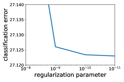
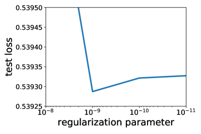
Figure 2: (Left) Classification error as a function of the regularization parameter and (Right) test loss as a function of the regularization parameter, when performing a logistic regression with $M=2\times 10^{4}$ Nyström features on the entire Higgs data set; we select $\lambda=10^{-9}$.

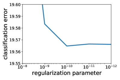
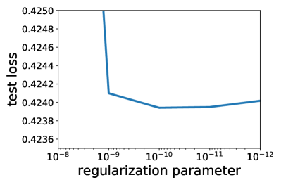
Figure 3: (Left) Classification error as a function of the regularization parameter and (Right) test loss as a function of the regularization parameter, when performing a logistic regression with $M=10^{4}$ Nyström features on the entire Susy data set; we select $\lambda=10^{-10}$.

Comparison with accelerated methods

Given the $M$ Nystrom points, our aims to minimize $\widehat{L}_{M,\lambda}$. From an optimization point of view, i.e. from a point of view where the aim is to minimize $\widehat{L}_{M,\lambda}$, we compare our method with a large mini-batch version of Katyusha accelerated SVRG (see [4]).
Indeed, we perform this method using batch sizes of size $M$; the theoretical bounds provided in [4] show that the algorithm has linear convergence, with a time complexity of order $O(nM+M^{3}+M^{2}\sqrt{\frac{L}{\lambda}})\log\frac{1}{\varepsilon}$ to reach precision $\varepsilon$. In the following plots, we compare both methods in terms of passes and time.

By pass, we mean the following.

• In the case of our second-order scheme, we define a pass on the data to be one step of the conjugate gradient descent used to compute approximate newton steps.

• In the case of Katyusha SVRG, we define a pass on the data to be either a full gradient computation or $n/M$ computations of the type $K_{\tau M}T^{-1}\beta$ where $T$ is an upper triangular matrix, and $K_{\tau M}$ is a $M\times M$ kernel matrix, associated to one batch gradient.

We use this notion to measure the speed of our method as they both correspond to natural $O(nM)$ operations, and incorporate the essential of the computing time. However, the second point is often much slower to compute than the first, due to the solving of the triangular system. Thus, the notion of passes is to take with precaution, as a pass for the accelerated SVRG algorithm takes much longer to run that a pass for our method. This is confirmed by the time plots (see Fig. 5 for in instance).

Comparison between the two methods - Due to the running time of K-SVRG, we compare both methods for $M=10000$ Nyström points for both data sets. We compare the performance of these two algorithm with respect to the distance to the optimum in function values as well as classification error Fig. 4 for the Higgs data set, and in Fig. 5 for the Susy data set.

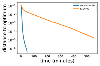
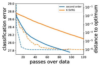
Figure 4: (Left) Distance to optimum as a function of time and (Right) distance to optimum and classification error as a function of the number of passes on the data when performing our second order scheme and K-SVRG to minimize the train loss on Higgs, with $1.0\times 10^{4}$ Nyström points and $\lambda=10^{-9}$.

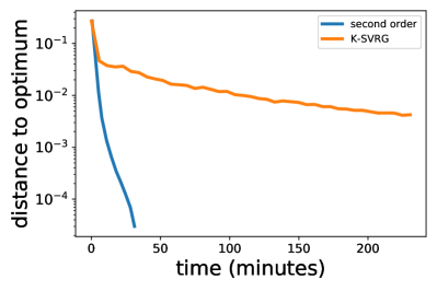
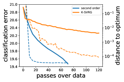
Figure 5: (Left) Distance to optimum as a function of time and (Right) distance to optimum and classification error as a function of the number of passes on the data when performing our second order scheme and K-SVRG to minimize the train loss on Susy, with $1.0\times 10^{4}$ Nyström points and $\lambda=10^{-10}$.

Note on the need for precise optimization - As noted in the introduction, we see in both Fig. 5 and Fig. 4 that precise optimization of the objective function is needed in order to get a good classification error. This justifies a posteriori the use of a second order method. In particular, in Fig. 5, one notes the difference in behavior between the two methods : the second order method converges linearly in a fast way while the first order method slows down because of the condition number.

Note on ill-conditioning - First note that in order to optimize test error, one gets very poorly conditioned problems. As predicted by the rates, we observe that K-SVRG is more sensible to ill-conditioning than our second order scheme. Indeed, in Fig. 6, we have plotted the results for Susy for a smaller condition number with $\lambda=10^{-8}$, compared to $\lambda=10^{-10}$ to get optimal test error in Fig. 5. We see that the difference in number of passes needed to reach a certain precision is much lower when $\lambda=10^{-8}$ in Fig. 6, confirming that K-SVRG behaves better when the condition number is smaller.

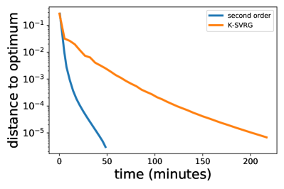
Figure 6: (Left) Distance to optimum as a function of time and (Right) distance to optimum and classification error as a function of the number of passes on the data when performing our second order scheme and K-SVRG to minimize the train loss on Susy, with $1.0\times 10^{4}$ Nyström points and $\lambda=10^{-8}$.

Performance of our method.

In Table 1, we record the performance of the following methods, taking the $\lambda$ values we have obtained previously for the different data sets.

For FALKON (see [29]), we take the parameters suggested in the paper (except for the number of Nyström points needed for Higgs, as our computational capacity is limited).

Method	Susy			Higgs
	c-error	$M$	time(m)	c-error	$M$	time(m)
Logistic regression with K-SVRG	19.64%	$10^{4}$	230	27.82 %	$10^{4}$	500
Logistic regression with our scheme	19.5%	$10^{4}$	15	26.9 %	$2.5\times 10^{4}$	65
Ridge Regression with FALKON ([29])	19.7%	$10^{4}$	5	27.16 %	$2.5\times 10^{4}$	60

Table 1: Classification error of different methods

Appendix G Solving a projected problem to reduce dimension

G.1 Introduction and notations

In this section, we give ourselves a generalized self-concordant function $f$ whose associated subset we denote with $\mathcal{G}$. Once again, we will always omit the subscript $f$ in the notations associated to $f$.

The aim of this section is the following. Given $f$ and $\lambda>0$, computing an approximate solution to

$$x_{\lambda}^{\star}=\operatorname*{arg\,min}_{x\in{\mathcal{H}}}{f_{\lambda}(x)},$$

is often too costly. Instead, we look for a solution in a small subset of ${\mathcal{H}}$ which we see as the image of a certain orthogonal projector $\mathbf{P}$ and which we denote ${\mathcal{H}}_{\mathbf{P}}$. Usually, this subset will be finite dimensional and admit an easy parametrization. Thus we will compare an approximation of $x_{\lambda}^{\star}$ to an approximation of

$$x_{\mathbf{P},\lambda}^{*}=\operatorname*{arg\,min}_{x\in{\mathcal{H}}_{\mathbf{P}}}{f_{\lambda}(x)}=\operatorname*{arg\,min}_{x\in{\mathcal{H}}}{f(\mathbf{P}x)+\frac{\lambda}{2}\|x\|^{2}}.$$

Denote with $f_{\mathbf{P}}$ the mapping $x\in{\mathcal{H}}\mapsto f(\mathbf{P}x)$. It is easy to see that, as $f$ is a generalized self-concordant function with $\mathcal{G}$, $f_{\mathbf{P}}$ is naturally a generalized self-concordant with $\mathcal{G}_{\mathbf{P}}:=\mathbf{P}\mathcal{G}=\left\{\mathbf{P}g\leavevmode\nobreak\ :\leavevmode\nobreak\ g\in\mathcal{G}\right\}$. Moreover, $x_{\mathbf{P},\lambda}^{*}=x^{\star}_{f_{\mathbf{P}},\lambda}$.

We will adopt the following notations for the quantities related to the generalized self-concordant function $f_{\mathbf{P}}$. Essentially, we always replace $f_{\mathbf{P}}$ simply by $\mathbf{P}$ from our definitions in appendix.

• For the regularized function :

  $$\forall x\in{\mathcal{H}},\leavevmode\nobreak\ \forall\lambda>0,\leavevmode\nobreak\ f_{\mathbf{P},\lambda}(x)=f_{\mathbf{P}}(x)+\frac{\lambda}{2}\|x\|^{2}.$$

• For the Hessians

  $$\forall x\in{\mathcal{H}},\leavevmode\nobreak\ \lambda>0,\leavevmode\nobreak\ \mathbf{H}_{\mathbf{P},\lambda}(x)=\mathbf{H}_{f_{\mathbf{P}},\lambda}(x)=\mathbf{P}\mathbf{H}(\mathbf{P}x)\mathbf{P}+\lambda\mathbf{I}.$$

• $\forall h\in{\mathcal{H}},\leavevmode\nobreak\ \mathsf{t}_{\mathbf{P}}(h):=\mathsf{t}_{f_{\mathbf{P}}}(h)=\mathsf{t}(\mathbf{P}h)$.

• For the Newton decrement:

  $$\forall x\in{\mathcal{H}},\leavevmode\nobreak\ \lambda>0,\leavevmode\nobreak\ \nu_{\mathbf{P},\lambda}(x)=\nu_{f_{\mathbf{P}},\lambda}(x)=\|\nabla f_{\mathbf{P},\lambda}\|_{\mathbf{H}^{-1}_{\mathbf{P},\lambda}(x)}=\|\mathbf{P}\nabla f(\mathbf{P}x)+\lambda x\|_{\mathbf{H}^{-1}_{\mathbf{P},\lambda}(x)}.$$

• For the Dikin ellipsoid radius:

  $$\forall\lambda>0,\leavevmode\nobreak\ \forall x\in{\mathcal{H}},\leavevmode\nobreak\ \mathsf{r}_{\mathbf{P},\lambda}(x):=\mathsf{r}_{f_{\mathbf{P}},\lambda}(x)=\frac{1}{\sup_{g\in\mathcal{G}}\|\mathbf{P}g\|_{\mathbf{H}_{\lambda,\mathbf{P}}^{-1}(x)}};$$

• For the Dikin ellipsoid:

  $$\forall\lambda>0,\leavevmode\nobreak\ \forall\mathsf{c}\geqslant 0,\leavevmode\nobreak\ \mathsf{D}_{\mathbf{P},\lambda}(\mathsf{c}):=\mathsf{D}_{f_{\mathbf{P}},\lambda}(\mathsf{c}).$$

Note that for any $x\in{\mathcal{H}}_{\mathbf{P}}$, $\mathsf{r}_{\mathbf{P},\lambda}(x)\geqslant\mathsf{r}_{\lambda}(x)$.

We will now introduce the key quantities in order to compare an approximation of $x_{\mathbf{P},\lambda}^{*}$ to an approximation of $x_{\lambda}^{\star}$.

Definition 8 (key quantities).

Define the following quantities

• For any $\lambda>0$, the source term $\mathsf{s}_{\lambda}:=\lambda\|x_{\lambda}^{\star}\|_{\mathbf{H}_{\lambda}^{-1}(x_{\lambda}^{\star})}=\|\nabla f(x_{\lambda}^{\star})\|_{\mathbf{H}_{\lambda}^{-1}(x_{\lambda}^{\star})}$;

• Given an orthogonal projector $\mathbf{P}$, $\lambda>0$, and $x\in{\mathcal{H}}$, the capacity of the projector $\mathsf{C}_{\mathbf{P}}(x,\lambda):=\frac{\|\mathbf{H}(x)^{1/2}(\mathbf{I}-\mathbf{P})\|^{2}}{\lambda}$.

G.2 Relating the projected to the original problem

Given $x\in{\mathcal{H}}_{\mathbf{P}}$, our aim is to bound $\nu_{\lambda}(x)$ given $\nu_{\lambda,\mathbf{P}}(x)$ and $\mathsf{s}_{\lambda}$.

Proposition 15.

Let $x\in{\mathcal{H}}_{\mathbf{P}}$. If

$$\frac{\mathsf{s}_{\lambda}}{\mathsf{r}_{\lambda}(x_{\lambda}^{\star})}\leqslant\frac{1}{4},\leavevmode\nobreak\ \mathsf{C}_{\mathbf{P}}(x_{\lambda}^{\star},\lambda)\leqslant\frac{1}{120},\leavevmode\nobreak\ \nu_{\mathbf{P},\lambda}(x)\leqslant\frac{\mathsf{r}_{\mathbf{P},\lambda}(x)}{2},$$

Then it holds:

$$\nu_{\lambda}(x)\leqslant 3(\nu_{\mathbf{P},\lambda}(x)+\mathsf{s}_{\lambda}).$$

Moreover, under these conditions,

• $\|x-x_{\lambda}^{\star}\|\leqslant 7\lambda^{-1/2}(\nu_{\mathbf{P},\lambda}(x)+\mathsf{s}_{\lambda})$;

• $\lambda\|x\|_{\mathbf{H}^{-1}_{\mathbf{P},\lambda}(x)}\leqslant 7\nu_{\mathbf{P},\lambda}(x)+9\mathsf{s}_{\lambda}$.

Proof.In this proof, introduce the following auxiliary quantity:

$$\gamma_{\lambda}:=\frac{\mathsf{s}_{\lambda}}{\mathsf{r}_{\lambda}(x_{\lambda}^{\star})}.$$

1) Start by bounding $\mathsf{t}(\mathbf{P}x_{\lambda}^{\star}-x_{\lambda}^{\star})$.

It holds:

$$\mathsf{t}(\mathbf{P}x-x_{\lambda}^{\star}) =\sup_{g\in\mathcal{G}}|g\cdot(\mathbf{I}-\mathbf{P})x_{\lambda}^{\star}|$$

$$\leqslant\frac{1}{\mathsf{r}_{\lambda}(x_{\lambda}^{\star})}\leavevmode\nobreak\ \|(\mathbf{I}-\mathbf{P})x_{\lambda}^{\star}\|_{\mathbf{H}_{\lambda}(x_{\lambda}^{\star})}$$

$$\leqslant\frac{1}{\mathsf{r}_{\lambda}(x_{\lambda}^{\star})}\leavevmode\nobreak\ \|\mathbf{H}_{\lambda}(x_{\lambda}^{\star})^{1/2}(\mathbf{I}-\mathbf{P})\mathbf{H}_{\lambda}(x_{\lambda}^{\star})^{1/2}\|\leavevmode\nobreak\ \|\mathbf{H}^{-1/2}_{\lambda}(x_{\lambda}^{\star})x_{\lambda}^{\star}\|$$

$$=\left(1+\mathsf{C}_{\mathbf{P}}(x_{\lambda}^{\star},\lambda)\right)\leavevmode\nobreak\ \frac{\lambda\|\mathbf{H}^{-1/2}_{\lambda}(x_{\lambda}^{\star})x_{\lambda}^{\star}\|}{\mathsf{r}_{\lambda}(x_{\lambda}^{\star})}$$

$$=(1+\mathsf{C}_{\mathbf{P}}(x_{\lambda}^{\star},\lambda))\leavevmode\nobreak\ \gamma_{\lambda}.$$

2) Then bound $\mathsf{t}(x_{\mathbf{P},\lambda}^{*}-\mathbf{P}x_{\lambda}^{\star})$

First, bound $\nu_{\mathbf{P},\lambda}(\mathbf{P}x_{\lambda}^{\star})$:

$$\nu_{\mathbf{P},\lambda}(\mathbf{P}x_{\lambda}^{\star}) =\|\mathbf{P}\nabla f_{\lambda}(\mathbf{P}x_{\lambda}^{\star})\|_{\mathbf{H}_{\lambda,\mathbf{P}}(\mathbf{P}x_{\lambda}^{\star})^{-1}}$$

$$\leqslant\|\nabla f_{\lambda}(\mathbf{P}x_{\lambda}^{\star})\|_{\mathbf{H}_{\lambda}(\mathbf{P}x_{\lambda}^{\star})^{-1}}.$$

Using Eq. 17, we get $\|\nabla f_{\lambda}(\mathbf{P}x_{\lambda}^{\star})\|_{\mathbf{H}_{\lambda}(\mathbf{P}x_{\lambda}^{\star})^{-1}}\leqslant e^{\mathsf{t}((\mathbf{I}-\mathbf{P})x_{\lambda}^{\star})/2}\nu_{\lambda}(\mathbf{P}x_{\lambda}^{\star})$. Using Eq. 20, we can bound

$$\nu_{\lambda}(\mathbf{P}x_{\lambda}^{\star})\leqslant\overline{\phi}(\mathsf{t}((\mathbf{I}-\mathbf{P})x_{\lambda}^{\star}))\leavevmode\nobreak\ \|(\mathbf{I}-\mathbf{P})x_{\lambda}^{\star}\|_{\mathbf{H}_{\lambda}(x_{\lambda}^{\star})}\leqslant\overline{\phi}(\mathsf{t}((\mathbf{I}-\mathbf{P})x_{\lambda}^{\star}))\leavevmode\nobreak\ (1+\mathsf{C}_{\mathbf{P}}(x_{\lambda}^{\star},\lambda))\mathsf{s}_{\lambda}.$$

Putting things together,

$$\nu_{\mathbf{P},\lambda}(\mathbf{P}x_{\lambda}^{\star})\leqslant e^{\mathsf{t}((\mathbf{I}-\mathbf{P})x_{\lambda}^{\star})/2}\overline{\phi}(\mathsf{t}((\mathbf{I}-\mathbf{P})x_{\lambda}^{\star}))\leavevmode\nobreak\ (1+\mathsf{C}_{\mathbf{P}}(x_{\lambda}^{\star},\lambda))\mathsf{s}_{\lambda}.$$

Now

$$\frac{1}{\mathsf{r}_{\mathbf{P},\lambda}(\mathbf{P}x_{\lambda}^{\star})}\leqslant\frac{1}{\mathsf{r}_{\lambda}(\mathbf{P}x_{\lambda}^{\star})}\leqslant e^{\mathsf{t}((\mathbf{I}-\mathbf{P})x_{\lambda}^{\star})/2}\frac{1}{\mathsf{r}_{\lambda}(x_{\lambda}^{\star})}.$$

Hence,

$$\frac{\nu_{\mathbf{P},\lambda}(\mathbf{P}x_{\lambda}^{\star})}{\mathsf{r}_{\mathbf{P},\lambda}(\mathbf{P}x_{\lambda}^{\star})}\leqslant e^{\tilde{t}_{\lambda}}\overline{\phi}(\tilde{t}_{\lambda})\leavevmode\nobreak\ \tilde{t}_{\lambda},\qquad\tilde{t}_{\lambda}=(1+\mathsf{C}_{\mathbf{P}}(x_{\lambda}^{\star},\lambda))\gamma_{\lambda}.$$

Since $t\mapsto e^{t}\overline{\phi}(t)\leavevmode\nobreak\ t$ is an increasing function whose value in $0$ is $0$, we find numerically that for $t=\frac{3}{10}$, $e^{t}\overline{\phi}(t)\leavevmode\nobreak\ t\leqslant\frac{1}{2}$. Hence, if $(1+\mathsf{C}_{\mathbf{P}}(x_{\lambda}^{\star},\lambda))\gamma_{\lambda}\leqslant\frac{3}{10}$, then $\frac{\nu_{\mathbf{P},\lambda}(\mathbf{P}x_{\lambda}^{\star})}{\mathsf{r}_{\mathbf{P},\lambda}(\mathbf{P}x_{\lambda}^{\star})}\leqslant\frac{1}{2}$. Using Lemma 5, this shows that

$$\mathsf{t}_{\mathbf{P}}(\mathbf{P}x_{\lambda}^{\star}-x_{\mathbf{P},\lambda}^{*})=\mathsf{t}(\mathbf{P}x_{\lambda}^{\star}-x_{\mathbf{P},\lambda}^{*})\leqslant\log 2.$$

3) Getting a bound for $\mathsf{t}(x-x_{\lambda}^{\star})$.

To do so, combine the two previous bounds with the fact that if $\nu_{\mathbf{P},\lambda}(x)\leqslant\frac{\mathsf{r}_{\mathbf{P},\lambda}(x)}{2}$, then using Lemma 5 with $f_{\mathbf{P}}$, $\mathsf{t}_{\mathbf{P}}(x-x_{\mathbf{P},\lambda}^{*})=\mathsf{t}(x-x_{\mathbf{P},\lambda}^{*})\leqslant\log 2$. Thus, if

$$(1+\mathsf{C}_{\mathbf{P}}(x_{\lambda}^{\star},\lambda))\gamma_{\lambda}\leqslant\frac{3}{10},\leavevmode\nobreak\ \nu_{\mathbf{P},\lambda}(x)\leqslant\frac{\mathsf{r}_{\mathbf{P},\lambda}(x)}{2},$$

then it holds

$$\mathsf{t}(x-x_{\lambda}^{\star})\leqslant\frac{3}{10}+2\log 2.$$

4) A technical result to bound $\|\mathbf{H}_{\lambda}(x)^{-1/2}\mathbf{H}_{\mathbf{P},\lambda}(x)^{1/2}\|$

. Using the fact that $\mathbf{P}x=x$, and Lemma 23, applied to $\mathbf{A}=\mathbf{H}(x)$, we get

$$\|\mathbf{H}_{\lambda}(x)^{-1/2}\mathbf{H}_{\mathbf{P},\lambda}(x)^{1/2}\|\leqslant 1+\sqrt{\mathsf{C}_{\mathbf{P}}(x,\lambda)}.$$

Then, one can easily bound $\mathsf{C}_{\mathbf{P}}(x,\lambda)\leqslant e^{\mathsf{t}(x-x_{\lambda}^{\star})}\mathsf{C}_{\mathbf{P}}(x_{\lambda}^{\star},\lambda)$.

5) Let us now bound $\nu_{\lambda}(x)$.

First, decompose the term

$$\nu_{\lambda}(x)=\|\nabla f_{\lambda}(x)\|_{\mathbf{H}^{-1}_{\lambda}(x)}\leqslant\|\mathbf{P}\nabla f_{\lambda}(x)\|_{\mathbf{H}^{-1}_{\lambda}(x)}+\|(\mathbf{I}-\mathbf{P})\nabla f(x)\|_{\mathbf{H}^{-1}_{\lambda}(x)}.$$

Since $x\in{\mathcal{H}}_{\mathbf{P}}$, $\|\mathbf{P}\nabla f_{\lambda}(x)\|_{\mathbf{H}^{-1}_{\lambda}(x)}=\|\nabla f_{\mathbf{P},\lambda}(x)\|_{\mathbf{H}^{-1}_{\lambda}(x)}$, and using the previous point, we get

$$\|\mathbf{P}\nabla f_{\lambda}(x)\|_{\mathbf{H}^{-1}_{\lambda}(x)}\leqslant\left(1+e^{\mathsf{t}(x-x_{\lambda}^{\star})/2}\sqrt{\mathsf{C}_{\mathbf{P}}(x_{\lambda}^{\star},\lambda)}\right)\nu_{\mathbf{P},\lambda}(x).$$

Let us now bound the second term. We divide it into two terms:

$$\|(\mathbf{I}-\mathbf{P})\nabla f(x)\|_{\mathbf{H}^{-1}_{\lambda}(x)}\leqslant\|(\mathbf{I}-\mathbf{P})\left(\nabla f(x)-\nabla f(x_{\lambda}^{\star})\right)\|_{\mathbf{H}^{-1}_{\lambda}(x)}+\|(\mathbf{I}-\mathbf{P})\nabla f(x_{\lambda}^{\star})\|_{\mathbf{H}^{-1}_{\lambda}(x)}.$$

The second term can be bounded in the following way:

$$\|(\mathbf{I}-\mathbf{P})\nabla f(x_{\lambda}^{\star})\|_{\mathbf{H}^{-1}_{\lambda}(x)}\leqslant\frac{1}{\sqrt{\lambda}}\|(\mathbf{I}-\mathbf{P})\mathbf{H}^{1/2}_{\lambda}(x_{\lambda}^{\star})\|\leavevmode\nobreak\ \|\nabla f(x_{\lambda}^{\star})\|_{\mathbf{H}^{-1}_{\lambda}(x_{\lambda}^{\star})}\leqslant\sqrt{1+\mathsf{C}_{\mathbf{P}}(x_{\lambda}^{\star},\lambda)}\leavevmode\nobreak\ \mathsf{s}_{\lambda}.$$

For the first term, we proceed in the following way.

$$\|(\mathbf{I}-\mathbf{P})\left(\nabla f(x)-\nabla f(x_{\lambda}^{\star})\right)\|_{\mathbf{H}^{-1}_{\lambda}(x)} =\|\int_{0}^{1}{\mathbf{H}_{\lambda}^{-1/2}(x)(\mathbf{I}-\mathbf{P})\mathbf{H}(x_{t})(x-x_{\lambda}^{\star})\leavevmode\nobreak\ dt}\|$$

$$\leqslant\frac{1}{\sqrt{\lambda}}\leavevmode\nobreak\ \int_{0}^{1}{\|(\mathbf{I}-\mathbf{P})\mathbf{H}^{1/2}(x_{t})\|\leavevmode\nobreak\ \|\mathbf{H}^{1/2}(x_{t})(x-x_{\lambda}^{\star})\|\leavevmode\nobreak\ dt}$$

$$\leqslant\sqrt{\mathsf{C}_{\mathbf{P}}(x_{\lambda}^{\star},\lambda)}\leavevmode\nobreak\ \overline{\phi}(\mathsf{t}(x-x_{\lambda}^{\star}))\leavevmode\nobreak\ \|x-x_{\lambda}^{\star}\|_{\mathbf{H}(x_{\lambda}^{\star})}$$

$$\leqslant\sqrt{\mathsf{C}_{\mathbf{P}}(x_{\lambda}^{\star},\lambda)}\leavevmode\nobreak\ e^{\mathsf{t}(x-x_{\lambda}^{\star})}\nu_{\lambda}(x).$$

Hence the final bound:

$$\left(1-\sqrt{\mathsf{C}_{\mathbf{P}}(x_{\lambda}^{\star},\lambda)}\leavevmode\nobreak\ e^{\mathsf{t}(x-x_{\lambda}^{\star})}\right)\nu_{\lambda}(x)\leqslant\left(1+e^{\mathsf{t}(x-x_{\lambda}^{\star})/2}\sqrt{\mathsf{C}_{\mathbf{P}}(x_{\lambda}^{\star},\lambda)}\right)\nu_{\mathbf{P},\lambda}(x)+\sqrt{1+\mathsf{C}_{\mathbf{P}}(x_{\lambda}^{\star},\lambda)}\leavevmode\nobreak\ \mathsf{s}_{\lambda}.$$

Now if $\mathsf{C}_{\mathbf{P}}(x_{\lambda}^{\star},\lambda)\leqslant\frac{1}{120}$, we see that $\sqrt{\mathsf{C}_{\mathbf{P}}(x_{\lambda}^{\star},\lambda)}\leavevmode\nobreak\ e^{\mathsf{t}(x-x_{\lambda}^{\star})}\leqslant\frac{1}{2}$, and hence, using the bound on $\mathsf{t}(x-x_{\lambda}^{\star})$,

$$\nu_{\lambda}(x)\leqslant 3(\nu_{\mathbf{P},\lambda}(x)+\mathsf{s}_{\lambda}).$$

6) Showing the last two points

. We leverage the fact that $\nu_{\lambda}(x)\leqslant 3(\nu_{\mathbf{P},\lambda}(x)+\mathsf{s}_{\lambda})$ and $\mathsf{t}(x-x_{\lambda}^{\star})\leqslant\frac{3}{10}+2\log 2$.
To show the first bound, we plug in the previous results in the following equation:

$$\|x-x_{\lambda}^{\star}\|\leqslant\lambda^{-1/2}\|x-x_{\lambda}^{\star}\|_{\mathbf{H}_{\lambda}(x)}\leqslant\frac{1}{\underline{\phi}(\mathsf{t}(x-x_{\lambda}^{\star}))}\leavevmode\nobreak\ \lambda^{-1/2}\nu_{\lambda}(x).$$

The last inequality is obtained using Eq. 18.

To show the second point, we use the fact that $x\in{\mathcal{H}}_{\mathbf{P}}$ to show that

$$\lambda\|x\|_{\mathbf{H}_{\mathbf{P},\lambda}^{-1}(x)}\leqslant\lambda\|x\|_{\mathbf{H}^{-1}_{\lambda}(x)}\leqslant\lambda\|x-x_{\lambda}^{\star}\|_{\mathbf{H}_{\lambda}(x)}+\lambda\|x_{\lambda}^{\star}\|_{\mathbf{H}^{-1}_{\lambda}(x)}.$$

Then applying Eq. 17 and Eq. 18:

$$\lambda\|x\|_{\mathbf{H}_{\mathbf{P},\lambda}^{-1}(x)}\leqslant\frac{1}{\underline{\phi}(\mathsf{t}(x-x_{\lambda}^{\star}))}\leavevmode\nobreak\ \nu_{\lambda}(x)+e^{\mathsf{t}(x-x_{\lambda}^{\star})/2}\mathsf{s}_{\lambda}.$$

We then use the previous results to conclude.

G.3 Finding a good projector

Lemma 16.

If for a certain $\eta\leqslant\lambda$ and for a certain constant $C$, $\|\mathbf{H}_{\eta}^{1/2}(x)(\mathbf{I}-\mathbf{P})\|^{2}\leqslant C\eta$, then

$$\mathsf{C}_{\mathbf{P}}(x,\lambda)\leqslant\frac{C\eta}{\lambda}.$$

Proof.This is completely direct, using the fact that $\mathbf{H}^{1/2}(x)\preceq\mathbf{H}_{\eta}^{1/2}(x)$.

Appendix H Relations between statistical problems and empirical problem.

In this section, we recall and reformulate the framework from [23].

H.1 Statistical problem and ERM estimator

Let $\mathcal{Z}$ be a Polish space and $Z$ be a random variable on $\mathcal{Z}$ with distribution $\rho$. Let ${\mathcal{H}}$ be a separable Hilbert space, with norm $\|\cdot\|$, and let $(f_{z})_{z\in\mathcal{Z}}$ be a family of functions on ${\mathcal{H}}$. Our goal is to minimize the expected risk with respect to $x\in{\mathcal{H}}$:

$$\inf_{x\in{\mathcal{H}}}\leavevmode\nobreak\ f(x):=\mathbb{E}\left[f_{Z}(x)\right].$$

Given $(z_{i})_{i=1}^{n}\in\mathcal{Z}^{n}$, we define the empirical risk:

$$\widehat{f}(x):=\frac{1}{n}\sum_{i=1}^{n}f_{z_{i}}(x),$$

and consider the following estimator based on regularized empirical risk minimization given $\lambda>0$ (note that the minimizer is unique in this case):

$$\widehat{x}_{\lambda}^{\star}=\operatorname*{arg\,min}_{x\in{\mathcal{H}}}\widehat{f}_{\lambda}(x):=\widehat{f}(x)+\frac{\lambda}{2}\|x\|^{2},$$

where we assume the following.

Assumption 6 (i.i.d. data).

The samples $(z_{i})_{1\leqslant i\leqslant n}$ are independently and identically distributed according to $\rho$.

We make the following assumption on the family $(f_{z})$ (this is a reformulation of Assumption 8 in [23])

Assumption 7 (Generalized self-concordance).

For any $z\in\mathcal{Z}$, there exists an associated subset $\mathcal{G}_{z}\subset{\mathcal{H}}$ such that $(f_{z},\mathcal{G}_{z})$ is generalized self-concordant in the sense of Definition 3.

Moreover we require the following technical assumption to guarantee that $f$ and and its derivatives are well defined for any $x\in{\mathcal{H}}$ (this is a reformulation of Assumptions 3 and 4 in [23], and the necessary conditions to obtain Proposition 3).

Assumption 8 (Technical assumptions).

The mapping $(z,x)\in\mathcal{Z}\times{\mathcal{H}}\mapsto f_{z}(x)$ is measurable. Moreover,

• the random variables $\|f_{Z}(0)\|,\|\nabla f_{Z}(0)\|,\operatorname{Tr}(\nabla^{2}f_{Z}(0))$ are are bounded;

• $\mathcal{G}:=\bigcup_{z\in\operatorname{supp}(Z)}\mathcal{G}_{z}$ is a bounded subset of ${\mathcal{H}}$.

The assumptions above are usually easy to check in practice. In particular, if the support of $\rho$ is bounded, the mappings $z\mapsto\ell_{z}(0),\nabla\ell_{z}(0),\operatorname{Tr}(\nabla^{2}\ell_{z}(0))$ are continuous, and $z\mapsto\mathcal{G}_{z}$ is uniformly bounded on bounded sets, then they hold.

Proposition 16.

Under Assumptions 7 and 8, the function $(f,\mathcal{G})$ (or simply $f$) is generalized self-concordant.

Moreover, under Assumption 6, define

$$\widehat{\mathcal{G}}:=\bigcup_{i=1}^{n}{\mathcal{G}_{z_{i}}}.$$

Then $(\widehat{f},\widehat{\mathcal{G}})$ (or simply $\widehat{f}$) is generalized self-concordant. Moreover, note that $\widehat{\mathcal{G}}\subset\mathcal{G}$.

The main regularity assumption we make on our statistical problems follows (see Assumption 5 in [23]).

Assumption 9 (Existence of a minimizer).

There exists $x^{\star}\in{\mathcal{H}}$ such that $f(x^{\star})=\inf_{x\in{\mathcal{H}}}f(x).$

Notations

We adopt all the notations from Appendix A for $f$ and $\widehat{f}$, which are generalized self-concordant functions with associated subsets given in Proposition 16 with the following conventions:

• For all quantities relating to $f$, we omit the subscript $f$ as usual;

• For all quantities relating to $\widehat{f}$, we omit the subscript $\widehat{f}$ and instead put a hat over all these quantities. For instance:

  $$\widehat{\mathbf{H}}(x):=\mathbf{H}_{\widehat{f}}(x)=\frac{1}{n}\sum_{i=1}^{n}{\nabla^{2}f_{z_{i}}(x)},\leavevmode\nobreak\ \widehat{\mathsf{r}}_{\lambda}(x):=\mathsf{r}_{\widehat{f},\lambda}(x)=\frac{1}{\sup_{g\in\widehat{\mathcal{G}}}{\|g\|_{\widehat{\mathbf{H}}^{-1}_{\lambda}(x)}}},\text{ etc...}$$

Recall the two main quantities introduced in [23] to establish the quality of our estimator $\widehat{x}_{\lambda}^{\star}$ (in [23], this is a mix between Proposition 2 and Definition 3).

Proposition 17 (Bias, degrees of freedom).

Suppose Assumptions 7, 8 and 9 are satisfied. The following key quantities are well defined:

• the bias $\mathsf{b}_{\lambda}=\|\mathbf{H}_{\lambda}(x^{\star})^{-1/2}\nabla f_{\lambda}(x^{\star})\|$;

• the effective dimension $\mathsf{df}_{\lambda}=\mathbb{E}\left[\|\mathbf{H}_{\lambda}(x^{\star})^{-1/2}\nabla f_{Z}(x^{\star})\|^{2}\right]$.

Moreover, we also introduce the following quantities:

$$\mathsf{B}_{1}^{\star}:=\sup_{z\in\operatorname{supp}(Z)}{\|\nabla f_{z}(x^{\star})\|},\qquad\mathsf{B}_{2}^{\star}:=\sup_{z\in\operatorname{supp}(Z)}{\operatorname{Tr}(\nabla^{2}f_{z}(x^{\star}))},\qquad\mathsf{Q}^{\star}=\frac{\mathsf{B}_{1}^{\star}}{\sqrt{\mathsf{B}_{2}^{\star}}}.$$

We can now recall the main theorem of [23] (Theorem 4), which quantifies the behavior of the ERM estimator:

Theorem 8 (Bound for the ERM estimator).

Let $n\in\mathbb{N}$, $\delta\in(0,1/2]$, $0<\lambda\leqslant\mathsf{B}_{2}^{\star}$. Whenever

$$n\geqslant\triangle_{1}\frac{\mathsf{B}_{2}^{\star}}{\lambda}\log\frac{8\square_{1}^{2}\mathsf{B}_{2}^{\star}}{\lambda\delta},\qquad\sqrt{\triangle_{2}\leavevmode\nobreak\ \frac{\mathsf{df}_{\lambda}\vee(\mathsf{Q}^{\star})^{2}}{n}\leavevmode\nobreak\ \log\frac{2}{\delta}}\leqslant\mathsf{r}_{\lambda}(x^{\star}),\qquad 2\mathsf{b}_{\lambda}\leqslant\mathsf{r}_{\lambda}(x^{\star}),$$

then with probability at least $1-2\delta$, it holds

$$f(\widehat{x}_{\lambda}^{\star})-f(x^{\star})\leqslant\mathsf{C}_{\textup{bias}}\leavevmode\nobreak\ \mathsf{b}_{\lambda}^{2}+\mathsf{C}_{\textup{var}}\leavevmode\nobreak\ \frac{\mathsf{df}_{\lambda}\vee(\mathsf{Q}^{\star})^{2}}{n}\leavevmode\nobreak\ \log\frac{2}{\delta},$$ (37)

where $\mathsf{C}_{\textup{bias}},\mathsf{C}_{\textup{var}},\square_{1}\leqslant 414,\leavevmode\nobreak\ \triangle_{1},\leavevmode\nobreak\ \triangle_{2}\leqslant 5184$.

H.2 Link between a good approximation of $\widehat{x}_{\lambda}^{\star}$ and $x^{\star}$

In this paper, we provide an algorithm which can effectively compute a good approximation of $\widehat{x}_{\lambda}^{\star}$ (as it is a finite sum problem which can be solved). This algorithm will return a certain $x\in{\mathcal{H}}$, whose precision with respect to the empirical problem will be characterized by $\widehat{\nu}_{\lambda}(x)$. The aim of the following lemma is to see how this approximation $x$ behaves with respect to the statistical problem.

Lemma 17.

Suppose the conditions for Thm. 8 are satisfied, i.e. let $n\in\mathbb{N}$, $\delta\in(0,1/2]$, $0<\lambda\leqslant\mathsf{B}_{2}^{\star}$ and suppose

$$n\geqslant\triangle_{1}\frac{\mathsf{B}_{2}^{\star}}{\lambda}\log\frac{8\square_{1}^{2}\mathsf{B}_{2}^{\star}}{\lambda\delta},\qquad\sqrt{\triangle_{2}\leavevmode\nobreak\ \frac{\mathsf{df}_{\lambda}\vee(\mathsf{Q}^{\star})^{2}}{n}\leavevmode\nobreak\ \log\frac{2}{\delta}}\leqslant\mathsf{r}_{\lambda}(x^{\star}),\qquad 2\mathsf{b}_{\lambda}\leqslant\mathsf{r}_{\lambda}(x^{\star}).$$

Let $x$ be an approximation of $\widehat{x}_{\lambda}^{\star}$ characterized by its Newton decrement $\widehat{\nu}_{\lambda}(x)$. If

$$\widehat{\nu}_{\lambda}(x)\leqslant\frac{\widehat{\mathsf{r}}_{\lambda}(x)}{2},\leavevmode\nobreak\ \widehat{\nu}_{\lambda}(x)\leqslant\frac{\mathsf{r}_{\lambda}(x^{\star})}{2},$$

then with probability at least $1-2\delta$, it holds

$$f(x)-f(x^{\star})\leqslant 14(f(\widehat{x}_{\lambda}^{\star})-f(x^{\star}))+30\widehat{\nu}_{\lambda}(x)^{2}.$$

Proof.Using Eq. 16,

$$f(x)-f(\widehat{x}_{\lambda}^{\star}) \leqslant\langle\nabla f(\widehat{x}_{\lambda}^{\star}),x-\widehat{x}_{\lambda}^{\star}\rangle_{{\mathcal{H}}}+\psi(\mathsf{t}(x-\widehat{x}_{\lambda}^{\star}))\|x-\widehat{x}_{\lambda}^{\star}\|_{\mathbf{H}_{\lambda}(\widehat{x}_{\lambda}^{\star})}^{2}$$

$$\leqslant\frac{1}{2}\|\nabla f(\widehat{x}_{\lambda}^{\star})\|^{2}_{\mathbf{H}^{-1}_{\lambda}(\widehat{x}_{\lambda}^{\star})}+\left(\psi(\mathsf{t}(x-\widehat{x}_{\lambda}^{\star}))+\frac{1}{2}\right)\|x-\widehat{x}_{\lambda}^{\star}\|^{2}_{\mathbf{H}_{\lambda}(\widehat{x}_{\lambda}^{\star})}.$$

1. Let us bound $\|\nabla f(\widehat{x}_{\lambda}^{\star})\|_{\mathbf{H}^{-1}_{\lambda}(\widehat{x}_{\lambda}^{\star})}$

$$\|\nabla f(\widehat{x}_{\lambda}^{\star})\|_{\mathbf{H}^{-1}_{\lambda}(\widehat{x}_{\lambda}^{\star})} \leqslant\int_{0}^{1}{\|\mathbf{H}^{-1/2}_{\lambda}(\widehat{x}_{\lambda}^{\star})\mathbf{H}(x_{t})(\widehat{x}_{\lambda}^{\star}-x^{\star})\|\leavevmode\nobreak\ dt}, x_{t}=(1-t)\widehat{x}_{\lambda}^{\star}+tx^{\star}$$

$$\leqslant\int_{0}^{1}{\|\mathbf{H}^{-1/2}_{\lambda}(\widehat{x}_{\lambda}^{\star})\mathbf{H}^{1/2}(x_{t})\|\leavevmode\nobreak\ \|\mathbf{H}^{1/2}(x_{t})(\widehat{x}_{\lambda}^{\star}-x^{\star})\|\leavevmode\nobreak\ dt}.$$

Now using equation Eq. 14

$$\mathbf{H}(x_{t})\preceq e^{t\mathsf{t}(\widehat{x}_{\lambda}^{\star}-x^{\star})}\mathbf{H}(\widehat{x}_{\lambda}^{\star}),\qquad\mathbf{H}(x_{t})\preceq e^{(1-t)\mathsf{t}(\widehat{x}_{\lambda}^{\star}-x^{\star})}.$$

Thus:

$$\|\nabla f(\widehat{x}_{\lambda}^{\star})\|_{\mathbf{H}^{-1}_{\lambda}(\widehat{x}_{\lambda}^{\star})}\leqslant e^{\mathsf{t}(\widehat{x}_{\lambda}^{\star}-x^{\star})/2}\leavevmode\nobreak\ \|\widehat{x}_{\lambda}^{\star}-x^{\star}\|_{\mathbf{H}(x^{\star})}.$$

Finally, using equation Eq. 16

$$\|\nabla f(\widehat{x}_{\lambda}^{\star})\|_{\mathbf{H}^{-1}_{\lambda}(\widehat{x}_{\lambda}^{\star})}\leqslant\frac{e^{\mathsf{t}(\widehat{x}_{\lambda}^{\star}-x^{\star})/2}}{\psi(-\mathsf{t}(\widehat{x}_{\lambda}^{\star}-x^{\star}))^{1/2}}\left(f(\widehat{x}_{\lambda}^{\star})-f(x^{\star})\right)^{1/2}.$$

2. Let us bound the terms involving $\|x-\widehat{x}_{\lambda}^{\star}\|_{\mathbf{H}_{\lambda}(\widehat{x}_{\lambda}^{\star})}$

Note that using Eq. 18 and Eq. 17 applied to $\widehat{f}$,

$$\|x-\widehat{x}_{\lambda}^{\star}\|_{\mathbf{H}_{\lambda}(\widehat{x}_{\lambda}^{\star})}\leqslant\|\mathbf{H}^{1/2}_{\lambda}(\widehat{x}_{\lambda}^{\star})\widehat{\mathbf{H}}^{-1/2}_{\lambda}(\widehat{x}_{\lambda}^{\star})\|\leavevmode\nobreak\ \frac{e^{\widehat{\mathsf{t}}(x-\widehat{x}_{\lambda}^{\star})/2}}{\underline{\phi}(\widehat{\mathsf{t}}(x-\widehat{x}_{\lambda}^{\star}))}\widehat{\nu}_{\lambda}(x).$$

This also leads to:

$$\mathsf{t}(x-\widehat{x}_{\lambda}^{\star}) \leqslant\frac{1}{\mathsf{r}_{\lambda}(\widehat{x}_{\lambda}^{\star})}\leavevmode\nobreak\ \|\mathbf{H}^{1/2}_{\lambda}(\widehat{x}_{\lambda}^{\star})\widehat{\mathbf{H}}^{-1/2}_{\lambda}(\widehat{x}_{\lambda}^{\star})\|\leavevmode\nobreak\ \|x-\widehat{x}_{\lambda}^{\star}\|_{\widehat{\mathbf{H}}_{\lambda}(\widehat{x}_{\lambda}^{\star})}$$

$$\leqslant\frac{1}{\mathsf{r}_{\lambda}(\widehat{x}_{\lambda}^{\star})}\leavevmode\nobreak\ \|\mathbf{H}^{1/2}_{\lambda}(\widehat{x}_{\lambda}^{\star})\widehat{\mathbf{H}}^{-1/2}_{\lambda}(\widehat{x}_{\lambda}^{\star})\|\leavevmode\nobreak\ \frac{e^{\widehat{\mathsf{t}}(x-\widehat{x}_{\lambda}^{\star})/2}}{\underline{\phi}(\widehat{\mathsf{t}}(x-\widehat{x}_{\lambda}^{\star}))}\widehat{\nu}_{\lambda}(x).$$

3. Putting things together

In the end, we get

$$f(x)-f(x^{\star}) \leqslant\left(1+\frac{e^{\mathsf{t}(\widehat{x}_{\lambda}^{\star}-x^{\star})}}{\psi(-\mathsf{t}(\widehat{x}_{\lambda}^{\star}-x^{\star}))}\right)(f(\widehat{x}_{\lambda}^{\star})-f(x^{\star}))$$

$$+\left(\psi(\mathsf{t}(x-\widehat{x}_{\lambda}^{\star}))+\frac{1}{2}\right)\left(e^{\mathsf{t}(\widehat{x}_{\lambda}^{\star}-x^{\star}_{\lambda})/2}\|\mathbf{H}^{1/2}_{\lambda}(x^{\star}_{\lambda})\widehat{\mathbf{H}}^{-1/2}_{\lambda}(x^{\star}_{\lambda})\|\frac{e^{\widehat{\mathsf{t}}(x-\widehat{x}_{\lambda}^{\star})/2}}{\underline{\phi}(\widehat{\mathsf{t}}(x-\widehat{x}_{\lambda}^{\star}))}\right)\leavevmode\nobreak\ \widehat{\nu}_{\lambda}(x)^{2}.$$

Moreover, we bound

$$\mathsf{t}(x-\widehat{x}_{\lambda}^{\star})\leqslant e^{(\mathsf{t}(x^{\star}-\widehat{x}_{\lambda}^{\star})+\mathsf{t}(\widehat{x}_{\lambda}^{\star}-x^{\star}_{\lambda}))/2}\leavevmode\nobreak\ \|\mathbf{H}^{1/2}_{\lambda}(x^{\star}_{\lambda})\widehat{\mathbf{H}}^{-1/2}_{\lambda}(x^{\star}_{\lambda})\|\leavevmode\nobreak\ \frac{e^{\widehat{\mathsf{t}}(x-\widehat{x}_{\lambda}^{\star})/2}}{\underline{\phi}(\widehat{\mathsf{t}}(x-\widehat{x}_{\lambda}^{\star}))}\frac{\widehat{\nu}_{\lambda}(x)}{\mathsf{r}_{\lambda}(x^{\star})}.$$

4. Plugging in previous results

Under the assumptions of this lemma, which include the assumptions of Theorem 4. in [23], we get the following bounds.

• In [23],the assumptions of Theorem 4 imply that we can use Lemma 9, which uses Lemma 8 in which we show that with probability at least $1-\delta$,

  $$\|\widehat{\mathbf{H}}_{\lambda}^{-1/2}(x_{\lambda}^{\star})\mathbf{H}_{\lambda}(x_{\lambda}^{\star})^{1/2}\|^{2}\leqslant 2.$$

• Still using the assumptions of Theorem 4, we see in the proof of this theorem that the assumptions of Theorem 7 of [23] are satisfied in the case where $\mathsf{b}_{\lambda}\leqslant\frac{\mathsf{r}_{\lambda}(x^{\star})}{2}$, and thus that

  $$\mathsf{t}(\widehat{x}_{\lambda}^{\star}-x^{\star}_{\lambda})\leqslant\log 2,\leavevmode\nobreak\ \mathsf{t}(x^{\star}_{\lambda}-x^{\star})\leqslant\log 2.$$

Plugging in all these bounds, we get

$$\left(1+\frac{e^{\mathsf{t}(\widehat{x}_{\lambda}^{\star}-x^{\star})}}{\psi(-\mathsf{t}(\widehat{x}_{\lambda}^{\star}-x^{\star}))}\right)\leqslant 14,\leavevmode\nobreak\ \mathsf{t}(x-\widehat{x}_{\lambda}^{\star})\leqslant 6,$$

$$\left(\psi(\mathsf{t}(x-\widehat{x}_{\lambda}^{\star}))+\frac{1}{2}\right)\left(e^{\mathsf{t}(\widehat{x}_{\lambda}^{\star}-x^{\star}_{\lambda})/2}\|\mathbf{H}^{1/2}_{\lambda}(x^{\star}_{\lambda})\widehat{\mathbf{H}}^{-1/2}_{\lambda}(x^{\star}_{\lambda})\|\frac{e^{\widehat{\mathsf{t}}(x-\widehat{x}_{\lambda}^{\star})/2}}{\underline{\phi}(\widehat{\mathsf{t}}(x-\widehat{x}_{\lambda}^{\star}))}\right)\leqslant 30.$$

H.3 Bounds when we solve a projected empirical problem

In this section, we place ourselves in the setting of Appendix G. In this section, we had argued that for computational purposes, it was less costly to compute an approximate solution to a projected problem.

In this section, we assume that we are going to project the regularized empirical problem, that is solve approximately

$$x\approx\operatorname*{arg\,min}_{x\in{\mathcal{H}}}{\widehat{f}_{\mathbf{P},\lambda}(x)}=\widehat{f}(\mathbf{P}x)+\frac{\lambda}{2}\|x\|^{2}.$$

for a given orthogonal projection $\mathbf{P}$. Recall from Appendix G that there is a natural way of seeing $\widehat{f}_{\mathbf{P}}$ as a generalized self-concordant function. We import all the notations from this section, keeping a $\widehat{\cdot}$ over all notations to mark the fact that we are projecting $\widehat{f}$ and not $f$.

To quantify the quality of the approximation $x$, we will use the Newton decrement for the empirical projected problem $\widehat{\nu}_{\mathbf{P},\lambda}(x):=\nu_{\widehat{f}_{\mathbf{P}},\lambda}(x)$.

As we see in Proposition 15, under certain conditions, bounding $\widehat{\nu}_{\lambda}(x)$ amounts to bounding two terms:

• The empirical source $\widehat{s}_{\lambda}:=\lambda\|\widehat{x}_{\lambda}^{\star}\|_{\widehat{\mathbf{H}}_{\lambda}^{-1}(\widehat{x}_{\lambda}^{\star})}$,

• The projected empirical Newton decrement $\widehat{\nu}_{\mathbf{P},\lambda}(x)$.

1. Bounding the empirical source term $\widehat{s}_{\lambda}$

Start by bounding the source empirical source term using quantities we know.

Lemma 18 (Empirical source).

Let $n\in\mathbb{N}$, $\delta\in(0,1/2]$, $0<\lambda\leqslant\mathsf{B}_{2}^{\star}$. Whenever

$$n\geqslant\triangle_{1}\frac{\mathsf{B}_{2}^{\star}}{\lambda}\log\frac{8\square_{1}^{2}\mathsf{B}_{2}^{\star}}{\lambda\delta},\qquad\sqrt{\triangle_{2}\leavevmode\nobreak\ \frac{\mathsf{df}_{\lambda}\vee(\mathsf{Q}^{\star})^{2}}{n}\leavevmode\nobreak\ \log\frac{2}{\delta}}\leqslant\mathsf{r}_{\lambda}(x^{\star}),\qquad 2\mathsf{b}_{\lambda}\leqslant\mathsf{r}_{\lambda}(x^{\star}).$$

The following holds, with probability at least $1-2\delta$.

$$\widehat{s}_{\lambda}\leqslant 8\leavevmode\nobreak\ \mathsf{b}_{\lambda}+80\leavevmode\nobreak\ \sqrt{\frac{\mathsf{df}_{\lambda}\vee(\mathsf{Q}^{\star})^{2}\leavevmode\nobreak\ \log\frac{2}{\delta}}{n}}.$$

Moreover, we also have the following bound :

$$\|\widehat{x}_{\lambda}^{\star}-x^{\star}\|\leqslant 3\leavevmode\nobreak\ \lambda^{-1/2}\leavevmode\nobreak\ \mathsf{b}_{\lambda}+8\leavevmode\nobreak\ \lambda^{-1/2}\leavevmode\nobreak\ \sqrt{\frac{\mathsf{df}_{\lambda}\vee(\mathsf{Q}^{\star})^{2}\leavevmode\nobreak\ \log\frac{2}{\delta}}{n}}.$$

Proof.

We first decompose the source term into two terms, and then apply different bounds from [23] to effectively bound it. We will use the following quantity:

$$\widehat{\mathsf{v}}_{\lambda}:=\|\mathbf{H}_{\lambda}^{1/2}(x_{\lambda}^{\star})\widehat{\mathbf{H}}_{\lambda}^{-1/2}(x_{\lambda}^{\star})\|^{2}\leavevmode\nobreak\ \|\nabla\widehat{f}_{\lambda}(x_{\lambda}^{\star})\|_{\mathbf{H}_{\lambda}^{-1}(x_{\lambda}^{\star})}.$$

It is also defined in equation (23) in [23].

1. Dividing $\widehat{s}_{\lambda}$ into two controllable terms

. Decompose

$$\widehat{s}_{\lambda}=\|\lambda\widehat{x}_{\lambda}^{\star}\|_{\widehat{\mathbf{H}}_{\lambda}^{-1}(\widehat{x}_{\lambda}^{\star})} \leqslant\|\widehat{\mathbf{H}}_{\lambda}^{-1/2}(\widehat{x}_{\lambda}^{\star})\mathbf{H}_{\lambda}^{1/2}(\widehat{x}_{\lambda}^{\star})\|\leavevmode\nobreak\ \|\lambda\widehat{x}_{\lambda}^{\star}\|_{\mathbf{H}_{\lambda}^{-1}(\widehat{x}_{\lambda}^{\star})}$$

$$\leqslant\|\widehat{\mathbf{H}}_{\lambda}^{-1/2}(\widehat{x}_{\lambda}^{\star})\mathbf{H}_{\lambda}^{1/2}(\widehat{x}_{\lambda}^{\star})\|\leavevmode\nobreak\ \left(\|\nabla f_{\lambda}(\widehat{x}_{\lambda}^{\star})\|_{\mathbf{H}^{-1}_{\lambda}(\widehat{x}_{\lambda}^{\star})}+\|\nabla f(\widehat{x}_{\lambda}^{\star})\|_{\mathbf{H}^{-1}_{\lambda}(\widehat{x}_{\lambda}^{\star})}\right).$$

On the one hand, from the previous proof, we get

$$\|\nabla f(\widehat{x}_{\lambda}^{\star})\|_{\mathbf{H}^{-1}_{\lambda}(\widehat{x}_{\lambda}^{\star})} \leqslant e^{\mathsf{t}(\widehat{x}_{\lambda}^{\star}-x^{\star})/2}\leavevmode\nobreak\ \|\widehat{x}_{\lambda}^{\star}-x^{\star}\|_{\mathbf{H}(x^{\star})}$$

$$\leqslant e^{\mathsf{t}(\widehat{x}_{\lambda}^{\star}-x^{\star})/2}\leavevmode\nobreak\ \left(e^{\mathsf{t}(x^{\star}_{\lambda}-x^{\star})}\|\widehat{x}_{\lambda}^{\star}-x^{\star}_{\lambda}\|_{\mathbf{H}_{\lambda}(x^{\star}_{\lambda})}+\|x^{\star}_{\lambda}-x^{\star}\|_{\mathbf{H}_{\lambda}(x^{\star})}\right)$$

$$\leqslant e^{\mathsf{t}(\widehat{x}_{\lambda}^{\star}-x^{\star})/2}\leavevmode\nobreak\ \left(\frac{e^{\mathsf{t}(x^{\star}_{\lambda}-x^{\star})}}{\underline{\phi}(\mathsf{t}(\widehat{x}_{\lambda}^{\star}-x^{\star}_{\lambda}))}\widehat{\mathsf{v}}_{\lambda}+\frac{1}{\underline{\phi}(\mathsf{t}(x^{\star}_{\lambda}-x^{\star}))}\mathsf{b}_{\lambda}\right).$$

In the last line, we use the fact that $\|\widehat{x}_{\lambda}^{\star}-x^{\star}_{\lambda}\|_{\mathbf{H}_{\lambda}(x^{\star}_{\lambda})}\leqslant\|\mathbf{H}^{1/2}_{\lambda}(x^{\star}_{\lambda})\widehat{\mathbf{H}}^{-1/2}_{\lambda}(x^{\star}_{\lambda})\|\leavevmode\nobreak\ \|\widehat{x}_{\lambda}^{\star}-x^{\star}_{\lambda}\|_{\widehat{\mathbf{H}}_{\lambda}(x^{\star}_{\lambda})}$ and then bound it using Eq. 18 applied to $\widehat{f}$ to get

$$\|\widehat{x}_{\lambda}^{\star}-x^{\star}_{\lambda}\|_{\widehat{\mathbf{H}}_{\lambda}(x^{\star}_{\lambda})} \leqslant\frac{1}{\underline{\phi}(\widehat{\mathsf{t}}(x_{\lambda}^{\star}-\widehat{x}_{\lambda}^{\star}))}\|\nabla\widehat{f}_{\lambda}(x_{\lambda}^{\star})\|_{\widehat{\mathbf{H}}_{\lambda}^{-1}(x_{\lambda}^{\star})}$$

$$\leqslant\frac{1}{\underline{\phi}(\mathsf{t}(x_{\lambda}^{\star}-\widehat{x}_{\lambda}^{\star}))}\|\mathbf{H}^{1/2}_{\lambda}(x^{\star}_{\lambda})\widehat{\mathbf{H}}^{-1/2}_{\lambda}(x^{\star}_{\lambda})\|\leavevmode\nobreak\ \|\nabla\widehat{f}_{\lambda}(x_{\lambda}^{\star})\|_{\mathbf{H}_{\lambda}^{-1}(x_{\lambda}^{\star})}.$$

On the other hand, apply successively Eq. 18 to $f$ and $\widehat{f}$ using the fact that $\widehat{\mathsf{t}}\leqslant\mathsf{t}$ to get

$$\|\nabla f_{\lambda}(\widehat{x}_{\lambda}^{\star})\|_{\mathbf{H}^{-1}_{\lambda}(\widehat{x}_{\lambda}^{\star})} =\|\nabla f_{\lambda}(\widehat{x}_{\lambda}^{\star})-\nabla f_{\lambda}(x^{\star}_{\lambda})\|_{\mathbf{H}^{-1}_{\lambda}(\widehat{x}_{\lambda}^{\star})}$$

$$\leqslant e^{\mathsf{t}(\widehat{x}_{\lambda}^{\star}-x^{\star}_{\lambda})/2}\overline{\phi}(\mathsf{t}(\widehat{x}_{\lambda}^{\star}-x^{\star}_{\lambda}))\leavevmode\nobreak\ \|\widehat{x}_{\lambda}^{\star}-x^{\star}_{\lambda}\|_{\mathbf{H}_{\lambda}(x^{\star}_{\lambda})}$$

$$\leqslant e^{\mathsf{t}(\widehat{x}_{\lambda}^{\star}-x^{\star}_{\lambda})/2}\overline{\phi}(\mathsf{t}(\widehat{x}_{\lambda}^{\star}-x^{\star}_{\lambda}))\leavevmode\nobreak\ \|\mathbf{H}^{1/2}_{\lambda}(x^{\star}_{\lambda})\widehat{\mathbf{H}}^{-1/2}_{\lambda}(x^{\star}_{\lambda})\|\leavevmode\nobreak\ \|\widehat{x}_{\lambda}^{\star}-x^{\star}_{\lambda}\|_{\widehat{\mathbf{H}}_{\lambda}(x^{\star}_{\lambda})}$$

$$\leqslant\frac{e^{\mathsf{t}(\widehat{x}_{\lambda}^{\star}-x^{\star}_{\lambda})/2}\overline{\phi}(\mathsf{t}(\widehat{x}_{\lambda}^{\star}-x^{\star}_{\lambda}))}{\underline{\phi}(\mathsf{t}(\widehat{x}_{\lambda}^{\star}-x^{\star}_{\lambda}))}\leavevmode\nobreak\ \|\mathbf{H}^{1/2}_{\lambda}(x^{\star}_{\lambda})\widehat{\mathbf{H}}^{-1/2}_{\lambda}(x^{\star}_{\lambda})\|^{2}\leavevmode\nobreak\ \|\nabla\widehat{f}_{\lambda}(x^{\star}_{\lambda})\|_{\mathbf{H}_{\lambda}(x^{\star}_{\lambda})}$$

$$=e^{3\mathsf{t}(\widehat{x}_{\lambda}^{\star}-x^{\star}_{\lambda})/2}\widehat{\mathsf{v}}_{\lambda}.$$

Putting things together:

$$\widehat{s}_{\lambda}\leqslant\|\widehat{\mathbf{H}}_{\lambda}^{-1/2}(\widehat{x}_{\lambda}^{\star})\mathbf{H}_{\lambda}^{1/2}(\widehat{x}_{\lambda}^{\star})\|\leavevmode\nobreak\ \left(e^{3\mathsf{t}(x_{\lambda}^{\star}-\widehat{x}_{\lambda}^{\star})/2}\left(1+\frac{1}{\underline{\phi}(\mathsf{t}(x_{\lambda}^{\star}-\widehat{x}_{\lambda}^{\star}))}\right)\widehat{\mathsf{v}}_{\lambda}+\frac{e^{\mathsf{t}(x_{\lambda}^{\star}-\widehat{x}_{\lambda}^{\star})/2}}{\underline{\phi}(\mathsf{t}(x_{\lambda}^{\star}-x^{\star}))}\mathsf{b}_{\lambda}\right).$$

2. We now import the results from [23]

. The following hypotheses imply those of Thms 4 and 7 in [23]:

Let $n\in\mathbb{N}$, $\delta\in(0,1/2]$, $0<\lambda\leqslant\mathsf{B}_{2}^{\star}$. Whenever

$$n\geqslant\triangle_{1}\frac{\mathsf{B}_{2}^{\star}}{\lambda}\log\frac{8\square_{1}^{2}\mathsf{B}_{2}^{\star}}{\lambda\delta},\leavevmode\nobreak\ \leavevmode\nobreak\ \leavevmode\nobreak\ n\geqslant\triangle_{2}\leavevmode\nobreak\ \frac{\mathsf{df}_{\lambda}\vee(\mathsf{Q}^{\star})^{2}}{\mathsf{r}_{\lambda}(x^{\star})^{2}}\leavevmode\nobreak\ \log\frac{2}{\delta},\mathsf{b}_{\lambda}\leqslant\frac{\mathsf{r}_{\lambda}(x^{\star})}{2}.$$

In particular, they imply that with probability at least $1-2\delta$:

• $\widehat{\mathsf{v}}_{\lambda}\leqslant\frac{1}{2}\mathsf{b}_{\lambda}+4\square_{1}\leavevmode\nobreak\ \sqrt{\frac{\mathsf{df}_{\lambda}\vee(\mathsf{Q}^{\star})^{2}\leavevmode\nobreak\ \log\frac{2}{\delta}}{n}}$;

• $\|\mathbf{H}^{1/2}_{\lambda}(x^{\star}_{\lambda})\widehat{\mathbf{H}}^{-1/2}_{\lambda}(x^{\star}_{\lambda})\|\leqslant\sqrt{2}$;

• $\mathsf{t}(x^{\star}-x^{\star}_{\lambda})\leqslant\log 2$;

• $\mathsf{t}(\widehat{x}_{\lambda}^{\star}-x^{\star}_{\lambda})\leqslant\log 2$.

Hence, plugging these bounds in the previous equation, we get

$$\widehat{s}_{\lambda}\leqslant 8\mathsf{b}_{\lambda}+80\sqrt{\frac{\mathsf{df}_{\lambda}\vee(\mathsf{Q}^{\star})^{2}\leavevmode\nobreak\ \log\frac{2}{\delta}}{n}}.$$

3.

Note that in what has been done previously, we can bound:

$$\|\widehat{x}_{\lambda}^{\star}-x_{\lambda}^{\star}\|_{\mathbf{H}_{\lambda}(x_{\lambda}^{\star})}\leqslant\frac{1}{\underline{\phi}(\mathsf{t}(x_{\lambda}^{\star}-\widehat{x}_{\lambda}^{\star}))}\widehat{\mathsf{v}}_{\lambda}\leqslant\mathsf{b}_{\lambda}+8\leavevmode\nobreak\ \sqrt{\frac{\mathsf{df}_{\lambda}\vee(\mathsf{Q}^{\star})^{2}\leavevmode\nobreak\ \log\frac{2}{\delta}}{n}}.$$

Moreover,

$$\|x_{\lambda}^{\star}-x^{\star}\|_{\mathbf{H}_{\lambda}(x^{\star})}\leqslant\frac{1}{\underline{\phi}(\mathsf{t}(x_{\lambda}^{\star}-x^{\star}))}\|\nabla f_{\lambda}(x^{\star})\|_{\mathbf{H}^{-1}_{\lambda}(x^{\star})}\leqslant 2\mathsf{b}_{\lambda}.$$

Hence:

$$\|\widehat{x}_{\lambda}^{\star}-x^{\star}\|\leqslant 3\leavevmode\nobreak\ \lambda^{-1/2}\leavevmode\nobreak\ \mathsf{b}_{\lambda}+8\leavevmode\nobreak\ \lambda^{-1/2}\leavevmode\nobreak\ \sqrt{\frac{\mathsf{df}_{\lambda}\vee(\mathsf{Q}^{\star})^{2}\leavevmode\nobreak\ \log\frac{2}{\delta}}{n}}.$$

2. Final bound for the projected ERM approximation

In this paragraph, denote with $\mathsf{C}_{\mathbf{P}}(x,\lambda)$ the quantity $\frac{\|\mathbf{H}^{1/2}(x)(\mathbf{I}-\mathbf{P})\|^{2}}{\lambda}$ and $\widehat{\mathsf{C}}_{\mathbf{P}}(x,\lambda)$ the quantity $\frac{\|\widehat{\mathbf{H}}^{1/2}(x)(\mathbf{I}-\mathbf{P})\|^{2}}{\lambda}$

Lemma 19.

Let $n\in\mathbb{N}$, $\delta\in(0,1/2]$, $0<\lambda\leqslant\mathsf{B}_{2}^{\star}$. Whenever

$$n\geqslant\triangle_{1}\frac{\mathsf{B}_{2}^{\star}}{\lambda}\log\frac{8\square_{1}^{2}\mathsf{B}_{2}^{\star}}{\lambda\delta},\qquad\mathsf{C}_{1}\sqrt{\frac{\mathsf{df}_{\lambda}\vee(\mathsf{Q}^{\star})^{2}}{n}\leavevmode\nobreak\ \log\frac{2}{\delta}}\leqslant\mathsf{r}_{\lambda}(x^{\star}),\qquad\mathsf{C}_{1}\mathsf{b}_{\lambda}\leqslant\mathsf{r}_{\lambda}(x^{\star}),$$

if

$$\mathsf{C}_{\mathbf{P}}(x^{\star},\lambda)\leqslant\frac{\sqrt{2}}{480},\leavevmode\nobreak\ \widehat{\nu}_{\mathbf{P},\lambda}(x)\leqslant\frac{\widehat{\mathsf{r}}_{\mathbf{P},\lambda}(x)}{2}\leavevmode\nobreak\ \wedge\leavevmode\nobreak\ \frac{\mathsf{r}_{\lambda}(x^{\star})}{126},$$

the following holds, with probability at least $1-2\delta$.

$$\widehat{\nu}_{\lambda}(x)\leqslant\frac{\widehat{\mathsf{r}}_{\lambda}(x)}{2},\leavevmode\nobreak\ \widehat{\nu}_{\lambda}(x)\leqslant\frac{\mathsf{r}_{\lambda}(x^{\star})}{2}.$$

Here, $\mathsf{C}_{1}=1008$.

Proof.

Proceed in the following way.

1.

It is easy to see that the conditions of this lemma imply the conditions of Thm. 8. Hence, as in the previous proofs, the following hold:

• $\|\mathbf{H}^{1/2}_{\lambda}(x^{\star}_{\lambda})\widehat{\mathbf{H}}^{-1/2}_{\lambda}(x^{\star}_{\lambda})\|\leqslant\sqrt{2}$;

• $\mathsf{t}(x^{\star}-x^{\star}_{\lambda})\leqslant\log 2$;

• $\mathsf{t}(\widehat{x}_{\lambda}^{\star}-x^{\star}_{\lambda})\leqslant\log 2$.

2.

Let us now apply Proposition 15 to $\widehat{f}$. If

$$\frac{\widehat{s}_{\lambda}}{\widehat{\mathsf{r}}_{\lambda}(\widehat{x}_{\lambda}^{\star})}\leqslant\frac{1}{4},\leavevmode\nobreak\ \widehat{\mathsf{C}}_{\mathbf{P}}(\widehat{x}_{\lambda}^{\star},\lambda)\leqslant\frac{1}{120},\leavevmode\nobreak\ \widehat{\nu}_{\mathbf{P},\lambda}(x)\leqslant\frac{\widehat{\mathsf{r}}_{\mathbf{P},\lambda}(x)}{2},$$

Then it holds:

$$\widehat{\nu}_{\lambda}(x)\leqslant 3(\widehat{\nu}_{\mathbf{P},\lambda}(x)+\widehat{s}_{\lambda}),\qquad\widehat{\mathsf{t}}(x-\widehat{x}_{\lambda}^{\star})\leqslant\frac{3}{10}+2\log 2.$$ (38)

where the second bound is obtained in the proof of this proposition. Now since

$$\frac{1}{\widehat{\mathsf{r}}_{\lambda}(\widehat{x}_{\lambda}^{\star})} \leqslant e^{\widehat{\mathsf{t}}(\widehat{x}_{\lambda}^{\star}-x_{\lambda}^{\star})/2}\frac{1}{\widehat{\mathsf{r}}_{\lambda}(x_{\lambda}^{\star})}$$

$$\leqslant e^{\widehat{\mathsf{t}}(\widehat{x}_{\lambda}^{\star}-x_{\lambda}^{\star})/2}\leavevmode\nobreak\ \|\mathbf{H}^{1/2}_{\lambda}(x^{\star}_{\lambda})\widehat{\mathbf{H}}^{-1/2}_{\lambda}(x^{\star}_{\lambda})\|\leavevmode\nobreak\ \sup_{g\in\widehat{\mathcal{G}}}{\|g\|_{\mathbf{H}^{-1}_{\lambda}(x_{\lambda}^{\star})}}$$ Def

$$\leqslant e^{\mathsf{t}(\widehat{x}_{\lambda}^{\star}-x_{\lambda}^{\star})/2}\leavevmode\nobreak\ \|\mathbf{H}^{1/2}_{\lambda}(x^{\star}_{\lambda})\widehat{\mathbf{H}}^{-1/2}_{\lambda}(x^{\star}_{\lambda})\|\leavevmode\nobreak\ \sup_{g\in\mathcal{G}}{\|g\|_{\mathbf{H}^{-1}_{\lambda}(x_{\lambda}^{\star})}} \widehat{\mathcal{G}}\subset\mathcal{G}$$

$$=e^{\mathsf{t}(\widehat{x}_{\lambda}^{\star}-x_{\lambda}^{\star})/2}\leavevmode\nobreak\ \|\mathbf{H}^{1/2}_{\lambda}(x^{\star}_{\lambda})\widehat{\mathbf{H}}^{-1/2}_{\lambda}(x^{\star}_{\lambda})\|\leavevmode\nobreak\ \frac{1}{\mathsf{r}_{\lambda}(x_{\lambda}^{\star})}$$ Def

$$\leqslant e^{(\mathsf{t}(\widehat{x}_{\lambda}^{\star}-x_{\lambda}^{\star})+\mathsf{t}(x_{\lambda}^{\star}-x^{\star}))/2}\leavevmode\nobreak\ \|\mathbf{H}^{1/2}_{\lambda}(x^{\star}_{\lambda})\widehat{\mathbf{H}}^{-1/2}_{\lambda}(x^{\star}_{\lambda})\|\leavevmode\nobreak\ \frac{1}{\mathsf{r}_{\lambda}(x^{\star})}$$

$$\leqslant\frac{2\sqrt{2}}{\mathsf{r}_{\lambda}(x^{\star})}.$$ previous bounds

In a similar way, we get $\widehat{\mathsf{C}}_{\mathbf{P}}(\widehat{x}_{\lambda}^{\star},\lambda)\leqslant 2\sqrt{2}\mathsf{C}_{\mathbf{P}}(x^{\star},\lambda)$. Thus, the conditions above are satisfied if the following conditions are satisfied:

$$\frac{\widehat{s}_{\lambda}}{\mathsf{r}_{\lambda}(x^{\star})}\leqslant\frac{\sqrt{2}}{16},\leavevmode\nobreak\ \mathsf{C}_{\mathbf{P}}(x^{\star},\lambda)\leqslant\frac{\sqrt{2}}{480},\leavevmode\nobreak\ \widehat{\nu}_{\mathbf{P},\lambda}(x)\leqslant\frac{\widehat{\mathsf{r}}_{\mathbf{P},\lambda}(x)}{2}.$$

Finally, note that under these conditions,

$$\frac{1}{\widehat{\mathsf{r}}_{\lambda}(x)}\leqslant\frac{e^{\widehat{\mathsf{t}}(x-\widehat{x}_{\lambda}^{\star})/2}}{\widehat{\mathsf{r}}_{\lambda}(x)}\leqslant\frac{7}{\mathsf{r}_{\lambda}(x^{\star})}.$$ (39)

using the previous bound and the bound on $\widehat{\mathsf{t}}(x-\widehat{x}_{\lambda}^{\star})$.

3.

Let us assume

$$\frac{\widehat{s}_{\lambda}}{\mathsf{r}_{\lambda}(x^{\star})}\leqslant\frac{\sqrt{2}}{16},\leavevmode\nobreak\ \mathsf{C}_{\mathbf{P}}(x^{\star},\lambda)\leqslant\frac{\sqrt{2}}{480},\leavevmode\nobreak\ \widehat{\nu}_{\mathbf{P},\lambda}(x)\leqslant\frac{\widehat{\mathsf{r}}_{\mathbf{P},\lambda}(x)}{2}.$$

According to Eq. 39, and to Eq. 38, if

$$\widehat{\nu}_{\mathbf{P},\lambda}(x)+\widehat{s}_{\lambda}\leqslant\frac{\mathsf{r}_{\lambda}(x^{\star})}{42},$$

then it holds

$$\widehat{\nu}_{\lambda}(x)\leqslant\frac{\widehat{\mathsf{r}}_{\lambda}(x)}{2},\leavevmode\nobreak\ \widehat{\nu}_{\lambda}(x)\leqslant\frac{\mathsf{r}_{\lambda}(x^{\star})}{2}.$$

We simplify this condition as:

$$\widehat{\nu}_{\mathbf{P},\lambda}(x)\leqslant\frac{\mathsf{r}_{\lambda}(x^{\star})}{126},\qquad\widehat{s}_{\lambda}\leqslant\frac{2\mathsf{r}_{\lambda}(x^{\star})}{126}.$$

4.

Now using the fact that under the conditions of this lemma, those of Lemma 18 are satisfied:

$$\widehat{s}_{\lambda}\leqslant 8\leavevmode\nobreak\ \mathsf{b}_{\lambda}+80\leavevmode\nobreak\ \sqrt{\frac{\mathsf{df}_{\lambda}\vee(\mathsf{Q}^{\star})^{2}\leavevmode\nobreak\ \log\frac{2}{\delta}}{n}}.$$

Thus, $\widehat{s}_{\lambda}\leqslant\frac{2\mathsf{r}_{\lambda}(x^{\star})}{126}$ holds, provided

$$\mathsf{b}_{\lambda}\leqslant\frac{\mathsf{r}_{\lambda}(x^{\star})}{\mathsf{C}_{1}},\leavevmode\nobreak\ n\geqslant\mathsf{C}_{1}^{2}\frac{\mathsf{df}_{\lambda}\vee(\mathsf{Q}^{\star})^{2}\leavevmode\nobreak\ \log\frac{2}{\delta}}{\mathsf{r}_{\lambda}(x^{\star})^{2}},$$

where $\mathsf{C}_{1}=1008$.

Proposition 18 (Behavior of an approximation to the projected problem).

Let $n\in\mathbb{N}$, $\delta\in(0,1/2]$, $0<\lambda\leqslant\mathsf{B}_{2}^{\star}$. Let $x\in{\mathcal{H}}_{\mathbf{P}}$. Whenever

$$n\geqslant\triangle_{1}\frac{\mathsf{B}_{2}^{\star}}{\lambda}\log\frac{8\square_{1}^{2}\mathsf{B}_{2}^{\star}}{\lambda\delta},\qquad\mathsf{C}_{1}\sqrt{\frac{\mathsf{df}_{\lambda}\vee(\mathsf{Q}^{\star})^{2}}{n}\leavevmode\nobreak\ \log\frac{2}{\delta}}\leqslant\mathsf{r}_{\lambda}(x^{\star}),\qquad\mathsf{C}_{1}\mathsf{b}_{\lambda}\leqslant\mathsf{r}_{\lambda}(x^{\star}),$$

if

$$\mathsf{C}_{\mathbf{P}}(x^{\star},\lambda)\leqslant\frac{\sqrt{2}}{480},\leavevmode\nobreak\ \widehat{\nu}_{\mathbf{P},\lambda}(x)\leqslant\frac{\widehat{\mathsf{r}}_{\mathbf{P},\lambda}(x)}{2}\leavevmode\nobreak\ \wedge\leavevmode\nobreak\ \frac{\mathsf{r}_{\lambda}(x^{\star})}{126}.$$

The following holds, with probability at least $1-2\delta$.

$$f(x)-f(x^{\star})\leqslant\mathsf{K}_{1}\leavevmode\nobreak\ \mathsf{b}_{\lambda}^{2}+\mathsf{K}_{2}\leavevmode\nobreak\ \frac{\mathsf{df}_{\lambda}\vee(\mathsf{Q}^{\star})^{2}}{n}\leavevmode\nobreak\ \log\frac{2}{\delta}+\mathsf{K}_{3}\leavevmode\nobreak\ \widehat{\nu}^{2}_{\mathbf{P},\lambda}(x),$$

where $\mathsf{K}_{1}\leqslant 6.0\mathrm{e}{4}$, $\mathsf{K}_{2}\leqslant 6.0\mathrm{e}{6}$ and $\mathsf{K}_{3}\leqslant 810$, $\mathsf{C}_{1}$ are defined in Lemma 19, and the other constants are defined in Thm. 8.

Remark 5 (Constants).

In this result, absolutely huge constants are obtained. They are (of course) totally sub-optimal. Indeed, this analysis has been simplified by dividing the bound into blocks: error of the empirical risk minimization with regularization, error of the projection compared to this empirical risk minimizer. Going back and forth from empirical to statistical, from projected to non projected induces exponential explosion of the constants. There is a way of doing the analysis directly by projecting the statistical problem. However, in order to relate to our previous work [23] and avoid re-doing all of our work we discarded this. If we were to perform this more direct analysis, we could keep the constants to a reasonable level, of order $10^{2}$.

Proof.We apply Lemma 17, using the previous lemma to guarantee the conditions.

1.

Under the conditions of this proposition, applying Lemma 19, the conditions of Lemma 17 are satisfied. Thus,

$$f(x)-f(x^{\star})\leqslant 14(f(\widehat{x}_{\lambda}^{\star})-f(x^{\star}))+30\widehat{\nu}_{\lambda}(x)^{2}.$$

Moreover, from the previous proof,

$$\widehat{\nu}_{\lambda}(x)\leqslant 3(\widehat{\nu}_{\mathbf{P},\lambda}(x)+\widehat{s}_{\lambda}),$$

and seeing as Lemma 18 is satisfied,

$$\widehat{s}_{\lambda}\leqslant 8\leavevmode\nobreak\ \mathsf{b}_{\lambda}+80\leavevmode\nobreak\ \sqrt{\frac{\mathsf{df}_{\lambda}\vee(\mathsf{Q}^{\star})^{2}\leavevmode\nobreak\ \log\frac{2}{\delta}}{n}}.$$

This therefore yields:

$$\widehat{\nu}_{\lambda}(x)^{2}\leqslant 27\widehat{\nu}_{\mathbf{P},\lambda}(x)^{2}+1726\mathsf{b}_{\lambda}^{2}+172600\frac{\mathsf{df}_{\lambda}\vee(\mathsf{Q}^{\star})^{2}\leavevmode\nobreak\ \log\frac{2}{\delta}}{n}.$$

2.

Moreover, from Thm. 8, it holds:

$$f(\widehat{x}_{\lambda}^{\star})-f(x^{\star})\leqslant 414\leavevmode\nobreak\ \mathsf{b}_{\lambda}^{2}+414\leavevmode\nobreak\ \frac{\mathsf{df}_{\lambda}\vee(\mathsf{Q}^{\star})^{2}}{n}\leavevmode\nobreak\ \log\frac{2}{\delta}.$$

3.

Putting things together:

$$f(x)-f(x^{\star})\leqslant\mathsf{K}_{1}\leavevmode\nobreak\ \mathsf{b}_{\lambda}^{2}+\mathsf{K}_{2}\leavevmode\nobreak\ \frac{\mathsf{df}_{\lambda}\vee(\mathsf{Q}^{\star})^{2}}{n}\leavevmode\nobreak\ \log\frac{2}{\delta}+\mathsf{K}_{3}\leavevmode\nobreak\ \widehat{\nu}^{2}_{\mathbf{P},\lambda}(x).$$

We bound the constants in the theorem.

Lemma 20.

Under the conditions of the previous theorem, the following hold:

• $\frac{1}{\widehat{\mathsf{r}}_{\mathbf{P},\lambda}(x)}\leqslant\frac{8}{\mathsf{r}_{\lambda}(x^{\star})}$;

• $\lambda^{1/2}\|x-x^{\star}\|\leqslant 7\widehat{\nu}_{\mathbf{P},\lambda}(x)+59\mathsf{b}_{\lambda}+568\sqrt{\frac{\mathsf{df}_{\lambda}\vee(\mathsf{Q}^{\star})^{2}\leavevmode\nobreak\ \log\frac{2}{\delta}}{n}}$;

• $\lambda\|x\|_{\widehat{\mathbf{H}}_{\mathbf{P},\lambda}^{-1}(x)}\leqslant 7\widehat{\nu}_{\mathbf{P},\lambda}(x)+72\mathsf{b}_{\lambda}+720\sqrt{\frac{\mathsf{df}_{\lambda}\vee(\mathsf{Q}^{\star})^{2}\leavevmode\nobreak\ \log\frac{2}{\delta}}{n}}$.

In particular, $\frac{\lambda\|x\|_{\widehat{\mathbf{H}}_{\mathbf{P},\lambda}^{-1}(x)}}{\widehat{\mathsf{r}}_{\mathbf{P},\lambda}(x)}\leqslant 11$.

Proof.Let us prove the three statements.

1.

Write $\frac{1}{\widehat{\mathsf{r}}_{\mathbf{P},\lambda}(x)}=\sup_{g\in\widehat{\mathcal{G}}}{\|\mathbf{P}g\|_{\widehat{\mathbf{H}}^{-1}_{\mathbf{P},\lambda}(x)}}$. Now

$$\sup_{g\in\widehat{\mathcal{G}}}{\|\mathbf{P}g\|_{\widehat{\mathbf{H}}^{-1}_{\mathbf{P},\lambda}(x)}}\leqslant\sup_{g\in\widehat{\mathcal{G}}}{\|g\|_{\widehat{\mathbf{H}}^{-1}_{\lambda}(x)}}\leqslant e^{\widehat{\mathsf{t}}(x-\widehat{x}_{\lambda}^{\star})/2}\sup_{g\in\widehat{\mathcal{G}}}{\|g\|_{\widehat{\mathbf{H}}^{-1}_{\lambda}(\widehat{x}_{\lambda}^{\star})}}.$$

Now bound

$$\sup_{g\in\widehat{\mathcal{G}}}{\|g\|_{\widehat{\mathbf{H}}^{-1}_{\lambda}(\widehat{x}_{\lambda}^{\star})}}\leqslant e^{\widehat{\mathsf{t}}(x_{\lambda}^{\star}-\widehat{x}_{\lambda}^{\star})/2}\sup_{g\in\widehat{\mathcal{G}}}{\|g\|_{\widehat{\mathbf{H}}^{-1}_{\lambda}(x_{\lambda}^{\star})}}\leqslant e^{\widehat{\mathsf{t}}(x_{\lambda}^{\star}-\widehat{x}_{\lambda}^{\star})/2}\leavevmode\nobreak\ \|\mathbf{H}^{1/2}_{\lambda}(x_{\lambda}^{\star})\widehat{\mathbf{H}}^{-1/2}_{\lambda}(x_{\lambda}^{\star})\|\leavevmode\nobreak\ \sup_{g\in\widehat{\mathcal{G}}}{\|g\|_{\mathbf{H}^{-1}_{\lambda}(x_{\lambda}^{\star})}}.$$

Finally bound

$$\sup_{g\in\widehat{\mathcal{G}}}{\|g\|_{\mathbf{H}^{-1}_{\lambda}(x_{\lambda}^{\star})}}\leqslant e^{\mathsf{t}(x^{\star}-x_{\lambda}^{\star})/2}\frac{1}{\mathsf{r}_{\lambda}(x^{\star})}.$$

Now using the fact that under the previous assumptions $\mathsf{t}(x^{\star}-x_{\lambda}^{\star}),\mathsf{t}(x_{\lambda}^{\star}-\widehat{x}_{\lambda}^{\star})\leqslant\log 2$, $\widehat{\mathsf{t}}(x-\widehat{x}_{\lambda}^{\star})\leqslant\frac{3}{10}+2\log 2$ and $\|\mathbf{H}^{1/2}_{\lambda}(x_{\lambda}^{\star})\widehat{\mathbf{H}}^{-1/2}_{\lambda}(x_{\lambda}^{\star})\|\leqslant\sqrt{2}$, we get the first equation.

2.

In order to bound $\lambda^{1/2}\|x-x^{\star}\|$, decompose

$$\lambda^{1/2}\|x-x^{\star}\|\leqslant\lambda^{1/2}\|x-\widehat{x}_{\lambda}^{\star}\|+\lambda^{1/2}\|\widehat{x}_{\lambda}^{\star}-x^{\star}\|.$$

Now use Proposition 15 to bound $\lambda^{1/2}\|x-\widehat{x}_{\lambda}^{\star}\|\leqslant 7(\widehat{\nu}_{\mathbf{P},\lambda}(x)+\widehat{s}_{\lambda})$. Using Lemma 18, under the conditions above,

$$\widehat{s}_{\lambda}\leqslant 8\leavevmode\nobreak\ \mathsf{b}_{\lambda}+80\leavevmode\nobreak\ \sqrt{\frac{\mathsf{df}_{\lambda}\vee(\mathsf{Q}^{\star})^{2}\leavevmode\nobreak\ \log\frac{2}{\delta}}{n}}.$$

Hence

$$\lambda^{1/2}\|x-\widehat{x}_{\lambda}^{\star}\|\leqslant 7\widehat{\nu}_{\mathbf{P},\lambda}(x)+56\mathsf{b}_{\lambda}+560\sqrt{\frac{\mathsf{df}_{\lambda}\vee(\mathsf{Q}^{\star})^{2}\leavevmode\nobreak\ \log\frac{2}{\delta}}{n}}.$$

Moreover, using again Lemma 18

$$\lambda^{1/2}\|\widehat{x}_{\lambda}^{\star}-x^{\star}\|\leqslant 3\leavevmode\nobreak\ \mathsf{b}_{\lambda}+8\leavevmode\nobreak\ \leavevmode\nobreak\ \sqrt{\frac{\mathsf{df}_{\lambda}\vee(\mathsf{Q}^{\star})^{2}\leavevmode\nobreak\ \log\frac{2}{\delta}}{n}}.$$

Combining these two inequalities, we get:

$$\lambda^{1/2}\|x-x^{\star}\|\leqslant 7\widehat{\nu}_{\mathbf{P},\lambda}(x)+59\mathsf{b}_{\lambda}+568\sqrt{\frac{\mathsf{df}_{\lambda}\vee(\mathsf{Q}^{\star})^{2}\leavevmode\nobreak\ \log\frac{2}{\delta}}{n}}.$$

3.

In order to bound $\lambda\|x\|_{\widehat{\mathbf{H}}_{\mathbf{P},\lambda}^{-1}(x)}$, use Proposition 15 to get $\lambda\|x\|_{\widehat{\mathbf{H}}^{-1}_{\mathbf{P},\lambda}(x)}\leqslant 7\widehat{\nu}_{\mathbf{P},\lambda}(x)+9\widehat{s}_{\lambda}$.

Now using Lemma 18, the following bound holds:

$$\lambda\|x\|_{\widehat{\mathbf{H}}_{\mathbf{P},\lambda}^{-1}(x)}\leqslant 7\widehat{\nu}_{\mathbf{P},\lambda}(x)+72\mathsf{b}_{\lambda}+720\sqrt{\frac{\mathsf{df}_{\lambda}\vee(\mathsf{Q}^{\star})^{2}\leavevmode\nobreak\ \log\frac{2}{\delta}}{n}}.$$

Proposition 19 (Simplification).

Let $n\in\mathbb{N}$, $\delta\in(0,1/2]$, $0<\lambda\leqslant\mathsf{B}_{2}^{\star}$. Let $x\in{\mathcal{H}}_{\mathbf{P}}$. Whenever

$$n\geqslant\triangle_{1}\frac{\mathsf{B}_{2}^{\star}}{\lambda}\log\frac{8\square_{1}^{2}\mathsf{B}_{2}^{\star}}{\lambda\delta},\qquad\mathsf{C}_{1}\sqrt{\frac{\mathsf{df}_{\lambda}\vee(\mathsf{Q}^{\star})^{2}}{n}\leavevmode\nobreak\ \log\frac{2}{\delta}}\leqslant\frac{\sqrt{\lambda}}{R},\qquad\mathsf{C}_{1}\mathsf{b}_{\lambda}\leqslant\frac{\sqrt{\lambda}}{R},$$

if

$$\mathsf{C}_{\mathbf{P}}(x^{\star},\lambda)\leqslant\frac{\sqrt{2}}{480},\leavevmode\nobreak\ \widehat{\nu}_{\mathbf{P},\lambda}(x)\leqslant\frac{\sqrt{\lambda}}{126R},$$

then the following holds, with probability at least $1-2\delta$.

$$f(x)-f(x^{\star})\leqslant\mathsf{K}_{1}\leavevmode\nobreak\ \mathsf{b}_{\lambda}^{2}+\mathsf{K}_{2}\leavevmode\nobreak\ \frac{\mathsf{df}_{\lambda}\vee(\mathsf{Q}^{\star})^{2}}{n}\leavevmode\nobreak\ \log\frac{2}{\delta}+\mathsf{K}_{3}\leavevmode\nobreak\ \widehat{\nu}^{2}_{\mathbf{P},\lambda}(x),$$

where $\mathsf{K}_{1}\leqslant 6.0\mathrm{e}{4}$, $\mathsf{K}_{2}\leqslant 6.0\mathrm{e}{6}$ and $\mathsf{K}_{3}\leqslant 810$, $\mathsf{C}_{1}$ are defined in Lemma 19, and the other constants are defined in Thm. 8.

Moreover, in that case, $R\|x-x^{\star}\|\leqslant 10$.

H.4 Optimal choice of $\lambda$, specific source conditions

In this part, we continue to assume Assumptions 7, 8, 6 and 9. We present a classification of distributions $\rho$ and show that we can achieve better rates than the classical slow rates, as presented in Appendix F of [23].

H.4.1 Classification of distributions and statistical bounds for the ERM

We use the following classification for distributions.

Definition 9 (class of distributions).

Let $\alpha\in[1,+\infty]$ and $r\in[0,1/2]$.
 We denote with $\mathcal{P}_{\alpha,r}$ the set of probability distributions $\rho$ such that there exists $\mathsf{L},\mathsf{Q}\geqslant 0$,

• $\mathsf{b}_{\lambda}\leqslant\mathsf{L}\leavevmode\nobreak\ \lambda^{\frac{1+2r}{2}}$;

• $\mathsf{df}_{\lambda}\leqslant\mathsf{Q}^{2}\leavevmode\nobreak\ \lambda^{-1/\alpha}$;

where this holds for any $0<\lambda\leqslant 1$. For simplicity, if $\alpha=+\infty$, we assume that $\mathsf{Q}\geqslant\mathsf{Q}^{\star}$.

Note that given our assumptions, we always have

$$\rho\in\mathcal{P}_{1,0},\leavevmode\nobreak\ \leavevmode\nobreak\ \leavevmode\nobreak\ \mathsf{L}=\|x^{\star}\|,\leavevmode\nobreak\ \mathsf{Q}=\mathsf{B}_{1}^{\star}.$$ (40)

We also define

$$\lambda_{1}=\left(\frac{\mathsf{Q}}{\mathsf{Q}^{\star}}\right)^{2\alpha}\wedge 1,$$ (41)

such that

$$\forall\lambda\leqslant\lambda_{1},\leavevmode\nobreak\ \mathsf{df}_{\lambda}\vee(\mathsf{Q}^{\star})^{2}\leqslant\frac{\mathsf{Q}^{2}}{\lambda^{1/\alpha}}.$$

Interpretation of the classes

• The bias term $\mathsf{b}_{\lambda}$ characterizes the regularity of the objective $x^{\star}$. In a sense, if $r$ is big, then this means $x^{\star}$ is very regular and will be easier to estimate. The following results reformulates this intuition.

  Remark 6 (source condition).

  Assume there exists $0\leqslant r\leqslant 1/2$ and $v\in{\mathcal{H}}$ such that

  $$\mathbf{P}_{\mathbf{H}(x^{\star})}x^{\star}=\mathbf{H}(x^{\star})^{r}v.$$

  Then it holds:

  $$\forall\lambda>0,\leavevmode\nobreak\ \mathsf{b}_{\lambda}\leqslant\mathsf{L}\leavevmode\nobreak\ \lambda^{\frac{1+2r}{2}},\leavevmode\nobreak\ \leavevmode\nobreak\ \leavevmode\nobreak\ \leavevmode\nobreak\ \mathsf{L}=\|\mathbf{H}(x^{\star})^{-r}x^{\star}\|.$$

• The effective dimension $\mathsf{df}_{\lambda}$ characterizes the size of the space ${\mathcal{H}}$ with respect to the problem. The higher $\alpha$, the smaller the space. If ${\mathcal{H}}$ is finite dimensional for instance, $\alpha=+\infty$.

In this section, for any given pair $(\alpha,r)$ characterizing the regularity and size of the problem, we associate

$$\beta=\frac{1}{1+2r+1/\alpha},\leavevmode\nobreak\ \leavevmode\nobreak\ \leavevmode\nobreak\ \leavevmode\nobreak\ \gamma=\frac{\alpha(1+2r)}{\alpha(1+2r)+1}.$$

In [23] (see corollary 3), explicit bounds are given for the performance of the regularized expected risk minimizer $\widehat{x}_{\lambda}^{\star}$ depending on which class $\rho$ belongs to, i.e., as a function of $\alpha,r$.

Corollary 4.

Let $\delta\in(0,1/2]$. Under Assumptions 7, 8, 6 and 9, if $\rho\in\mathcal{P}_{\alpha,r}$ with $r>0$ , when $n\geqslant N$ and $\lambda=(C_{0}/n)^{\beta}$, then with probability at least $1-2\delta$,

$$f(\widehat{x}_{\lambda}^{\star})-f(x^{\star})\leqslant C_{1}n^{-\gamma}\log\frac{2}{\delta},$$

with $C_{0}=256(\mathsf{Q}/\mathsf{L})^{2},\leavevmode\nobreak\ C_{1}=8(256)^{\gamma}\leavevmode\nobreak\ (\mathsf{Q}^{\gamma}\leavevmode\nobreak\ \mathsf{L}^{1-\gamma})^{2}$ and $N$ defined in [23], and satisfying $N=O(\operatorname{poly}(\mathsf{B}_{1}^{\star},\mathsf{B}_{2}^{\star},\mathsf{L},\mathsf{Q},R,\log(1/\delta)))$.

H.4.2 Quantitative bounds for the projected problem

In this part, the aim is to show that if we approximately solve the projected problem up to a certain precision, then this approximation has the same statistical rates as the regularized ERM with the good choice of $\lambda$. For the sake of simplicity, we will assume that $r>0$.

In what follows, we define

$$N=\frac{\mathsf{Q}^{2}}{\mathsf{L}^{2}}\left(\mathsf{B}_{2}^{\star}\wedge\lambda_{0}\wedge\lambda_{1}\right)^{-1/\beta}\leavevmode\nobreak\ \leavevmode\nobreak\ \leavevmode\nobreak\ \vee\leavevmode\nobreak\ \leavevmode\nobreak\ \leavevmode\nobreak\ \left(2.1e4\frac{1}{1-\beta}A\log\left(1.4e6\frac{1}{1-\beta}A^{2}\frac{1}{\delta}\right)\right)^{1/(1-\beta)},$$ (42)

where $A=\frac{\mathsf{B}_{2}^{\star}\mathsf{L}^{2\beta}}{\mathsf{Q}^{2\beta}}$, $\lambda_{0}=(\mathsf{C}_{1}\mathsf{L}R\log\frac{2}{\delta})^{-1/r}\wedge 1$ and $\lambda_{1}=\frac{\mathsf{Q}^{2\alpha}}{(\mathsf{Q}^{\star})^{2\alpha}}$.

Theorem 9 (Quantitative result with source $r>0$).

Let $\rho\in\mathcal{P}_{\alpha,r}$ and assume $r>0$. Let $\delta\in(0,\frac{1}{2}]$.
 Let $\mathbf{P}$ be an orthogonal projection, $x\in{\mathcal{H}}$. If

$$n\geqslant N,\leavevmode\nobreak\ \leavevmode\nobreak\ \leavevmode\nobreak\ \lambda=\left(\left(\frac{\mathsf{Q}}{\mathsf{L}}\right)^{2}\leavevmode\nobreak\ \frac{1}{n}\right)^{\beta},\leavevmode\nobreak\ \leavevmode\nobreak\ \leavevmode\nobreak\ \leavevmode\nobreak\ \mathsf{C}_{\mathbf{P}}(x^{\star},\lambda)\leqslant\frac{\sqrt{2}}{480},\leavevmode\nobreak\ \widehat{\nu}_{\mathbf{P},\lambda}(x)\leqslant\mathsf{Q}^{\gamma}\leavevmode\nobreak\ \mathsf{L}^{1-\gamma}n^{-\gamma/2}$$

then with probability at least $1-2\delta$,

$$f(x)-f(x^{\star})\leqslant\mathsf{K}\left(\mathsf{Q}^{\gamma}\leavevmode\nobreak\ \mathsf{L}^{1-\gamma}\right)^{2}\leavevmode\nobreak\ \leavevmode\nobreak\ \frac{1}{n^{\gamma}}\log\frac{2}{\delta},$$

where $N$ is defined in Eq. 42 and $\mathsf{K}\leqslant 7.0e6$. Moreover, $R\|x-x^{\star}\|\leqslant 10$.

Proof.

Using the definition of $\lambda_{1}$, as soon as $\lambda\leqslant\lambda_{1}$ ,it holds: $\mathsf{df}_{\lambda}\vee(\mathsf{Q}^{\star})^{2}\leqslant\mathsf{Q}^{2}\lambda^{-1/\alpha}$.

Let us formulate Proposition 19 using the fact that $\rho\in\mathcal{P}_{\alpha,r}$.

Let $n\in\mathbb{N}$, $\delta\in(0,1/2]$, $0<\lambda\leqslant\mathsf{B}_{2}^{\star}$, $x\in{\mathcal{H}}_{\mathbf{P}}$. Whenever

$$n\geqslant\triangle_{1}\frac{\mathsf{B}_{2}^{\star}}{\lambda}\log\frac{8\square_{1}^{2}\mathsf{B}_{2}^{\star}}{\lambda\delta},\leavevmode\nobreak\ \leavevmode\nobreak\ \leavevmode\nobreak\ \mathsf{C}_{1}\sqrt{\frac{\mathsf{Q}^{2}}{\lambda^{1/\alpha}n}\leavevmode\nobreak\ \log\frac{2}{\delta}}\leqslant\frac{\lambda^{1/2}}{R},\mathsf{C}_{1}\leavevmode\nobreak\ \mathsf{L}\lambda^{1/2+r}\leqslant\frac{\lambda^{1/2}}{R},$$

if

$$\mathsf{C}_{\mathbf{P}}(x^{\star},\lambda)\leqslant\frac{\sqrt{2}}{480},\leavevmode\nobreak\ \widehat{\nu}_{\mathbf{P},\lambda}(x)\leqslant\mathsf{L}\lambda^{1/2+r},$$

The following holds, with probability at least $1-2\delta$.

$$f(x)-f(x^{\star})\leqslant(\mathsf{K}_{1}+\mathsf{K}_{3})\mathsf{L}^{2}\lambda^{1+2r}+\mathsf{K}_{2}\leavevmode\nobreak\ \frac{\mathsf{Q}^{2}}{\lambda^{1/\alpha}n}\leavevmode\nobreak\ \log\frac{2}{\delta},\qquad R\|x-x^{\star}\|\leqslant 10,$$

where all constants are defined in Proposition 19.

Assume that $r>0$

. Define

$$\lambda_{0}=(\mathsf{C}_{1}\mathsf{L}R\log\frac{2}{\delta})^{-1/r}\wedge 1.$$

Then for any $\lambda\leqslant\lambda_{0}$:

$$\mathsf{L}\lambda^{1/2+r}\leqslant\frac{1}{\mathsf{C}_{1}}\frac{\sqrt{\lambda}}{R}.$$

1) First, we find a simple condition to guarantee

$$\mathsf{r}_{\lambda}(x^{\star})^{2}\lambda^{1/\alpha}\geqslant\mathsf{C}_{2}\leavevmode\nobreak\ \mathsf{Q}^{2}\frac{1}{n}\leavevmode\nobreak\ \log\frac{2}{\delta}.$$

We see that if $\lambda\leqslant\lambda_{0}$, then $\mathsf{r}_{\lambda}\geqslant\mathsf{C}_{1}\mathsf{L}\lambda^{1/2+r}\log\frac{2}{\delta}$. Hence, this condition is satisfied if

$$\lambda\leqslant\lambda_{0},\leavevmode\nobreak\ \leavevmode\nobreak\ \leavevmode\nobreak\ \leavevmode\nobreak\ \mathsf{C}_{1}^{2}\mathsf{L}^{2}\lambda^{1+2r+1/\alpha}\geqslant\mathsf{C}_{2}\leavevmode\nobreak\ \mathsf{Q}^{2}\frac{1}{n}.$$

Using the fact that $\mathsf{C}_{2}=\mathsf{C}_{1}^{2}$, we reformulate:

$$\lambda\leqslant\lambda_{0},\leavevmode\nobreak\ \leavevmode\nobreak\ \leavevmode\nobreak\ \leavevmode\nobreak\ \mathsf{L}^{2}\lambda^{1+2r+1/\alpha}\geqslant\mathsf{Q}^{2}\frac{1}{n}.$$

2) Now fix

$$\lambda^{1+2r+1/\alpha}=\frac{\mathsf{Q}^{2}}{\mathsf{L}^{2}}\leavevmode\nobreak\ \frac{1}{n}\Longleftrightarrow\lambda=\left(\frac{\mathsf{Q}^{2}}{\mathsf{L}^{2}}\leavevmode\nobreak\ \frac{1}{n}\right)^{\beta}.$$

where $\beta=1/(1+2r+1/\lambda)\in[1/2,1)$.

Using our restatement of Proposition 18, with probability at least $1-2\delta$,

$$L(x)-L(x^{\star})\leqslant\left(\mathsf{K}_{1}+\mathsf{K}_{3}+\mathsf{K}_{2}\log\frac{2}{\delta}\right)\leavevmode\nobreak\ \mathsf{L}^{2}\lambda^{1+2r}\leqslant\mathsf{K}\leavevmode\nobreak\ \log\frac{2}{\delta}\leavevmode\nobreak\ \mathsf{L}^{2}\lambda^{1+2r},$$

where $\mathsf{K}=\mathsf{K}_{1}+\mathsf{K}_{3}+\mathsf{K}_{2}\leqslant 7.0e6$ (see Proposition 18).
 This result holds provided

$$0<\lambda\leqslant\mathsf{B}_{2}^{\star}\wedge\lambda_{0}\wedge\lambda_{1},\leavevmode\nobreak\ n\geqslant\triangle_{1}\frac{\mathsf{B}_{2}^{\star}}{\lambda}\log\frac{8\square_{1}^{2}\mathsf{B}_{2}^{\star}}{\lambda\delta}.$$ (43)

Indeed, it is shown in the previous point that the other conditions are satisfied.

3) Let us now work to guarantee the conditions in Eq. 43.
 First, to guarantee $n\geqslant\triangle_{1}\frac{\mathsf{B}_{2}^{\star}}{\lambda}\log\frac{8\square_{1}^{2}\mathsf{B}_{2}^{\star}}{\lambda\delta}$, bound

$$\frac{\mathsf{B}_{2}^{\star}}{\lambda}=\frac{\mathsf{B}_{2}^{\star}\mathsf{L}^{2\beta}n^{\beta}}{\mathsf{Q}^{2\beta}\leavevmode\nobreak\ \log^{\beta}\frac{2}{\delta}}\leqslant 2\leavevmode\nobreak\ \frac{\mathsf{B}_{2}^{\star}\mathsf{L}^{2\beta}}{\mathsf{Q}^{2\beta}}n^{\beta}.$$

Then apply lemma 15 from [23] with $a_{1}=2\triangle_{1}$, $a_{2}=16\square_{1}^{2}$, $A=\frac{\mathsf{B}_{2}^{\star}\mathsf{L}^{2\beta}}{\mathsf{Q}^{2\beta}}$. Since $\beta\geqslant 1/2$, using the bounds in Thm. 8, we find $a_{1}\leqslant 10400$ and $a_{2}\leqslant 64,$ hence the following sufficient condition:

$$n\geqslant\left(2.1e4\frac{1}{1-\beta}A\log\left(1.4e6\frac{1}{1-\beta}A^{2}\frac{1}{\delta}\right)\right)^{1/(1-\beta)}.$$

Then, to guarantee the condition

$$\lambda\leqslant\mathsf{B}_{2}^{\star}\wedge\lambda_{0}\wedge\lambda_{1},$$

we simply need

$$n\geqslant\frac{\mathsf{Q}^{2}}{\mathsf{L}^{2}}\left(\mathsf{B}_{2}^{\star}\wedge\lambda_{0}\wedge\lambda_{1}\right)^{-1/\beta}.$$

Hence, defining

$$N=\frac{\mathsf{Q}^{2}}{\mathsf{L}^{2}}\left(\mathsf{B}_{2}^{\star}\wedge\lambda_{0}\wedge\lambda_{1}\right)^{-1/\beta}\leavevmode\nobreak\ \leavevmode\nobreak\ \leavevmode\nobreak\ \vee\leavevmode\nobreak\ \leavevmode\nobreak\ \leavevmode\nobreak\ \left(2.1e4\frac{1}{1-\beta}A\log\left(1.4e6\frac{1}{1-\beta}A^{2}\frac{1}{\delta}\right)\right)^{1/(1-\beta)},$$

we see that as soon as $n\geqslant N$, Eq. 43 holds.

Appendix I Multiplicative approximations for Hermitian operators

In this section, we put together useful tools for approximating linear operators and solving linear systems with regularization.

In this section, $\mathbf{A}$ and $\mathbf{B}$ will always denote positive semi-definite Hermitian operators on a Hilbert space ${\mathcal{H}}$, and $\mathbf{P}$ will denote an orthogonal projection operator. Moreover, given a positive semi-definite operator $\mathbf{A}$, and $\lambda>0$, $\mathbf{A}_{\lambda}$ will stand for the regularized operator $\mathbf{A}+\lambda\mathbf{I}$.

Lemma 21 (Equivalence of Hermitian operators).

Let $\mathbf{A}$ and $\mathbf{B}$ be two semi-definite Hermitian operators. Let $\lambda>0$. Assume you have access to

$$t:=\|\mathbf{A}_{\lambda}^{-1/2}(\mathbf{B}-\mathbf{A})\mathbf{A}^{-1/2}_{\lambda}\|.$$

It holds:

$$\|\mathbf{A}_{\lambda}^{-1/2}\mathbf{B}_{\lambda}^{1/2}\|^{2}\leqslant 1+t\Leftrightarrow\mathbf{B}_{\lambda}\preceq(1+t)\mathbf{A}_{\lambda}.$$

Moreover, if $t<1$,

$$\|\mathbf{B}_{\lambda}^{-1/2}\mathbf{A}_{\lambda}^{1/2}\|^{2}\leqslant\frac{1}{1-t}\Leftrightarrow(1-t)\mathbf{A}_{\lambda}\preceq\mathbf{B}_{\lambda}.$$

Proof.For the first point, simply note that:

$$\|\mathbf{A}_{\lambda}^{-1/2}\mathbf{B}_{\lambda}^{1/2}\|^{2}=\|\mathbf{A}_{\lambda}^{-1/2}\mathbf{B}_{\lambda}\mathbf{A}_{\lambda}^{-1/2}\|=\|\mathbf{I}+\mathbf{A}_{\lambda}^{-1/2}\left(\mathbf{B}-\mathbf{A}\right)\mathbf{A}_{\lambda}^{-1/2}\|\leqslant 1+t.$$

For the second point,

$$\|\mathbf{B}_{\lambda}^{-1/2}\mathbf{A}_{\lambda}^{1/2}\|^{2}=\|\left(\mathbf{A}_{\lambda}^{-1/2}\mathbf{B}_{\lambda}\mathbf{A}_{\lambda}^{-1/2}\right)^{-1}\|=\|\left(\mathbf{I}+\mathbf{A}_{\lambda}^{-1/2}\left(\mathbf{B}-\mathbf{A}\right)\mathbf{A}_{\lambda}^{-1/2}\right)^{-1}\|.$$

Moreover, we know that if $\|\mathbf{H}\|<1$ with $\mathbf{H}$ a Hermitian operator, then $\|(\mathbf{I}+\mathbf{H})^{-1}\|\leqslant\frac{1}{1-\|\mathbf{H}\|}$. The result follows.

We will now state a technical lemma which describes how combining approximation behaves.

Lemma 22 (Combination of approximations).

Let $N\geqslant 1$. Let $(\mathbf{A}_{i})_{1\leqslant i\leqslant N+1}$ be a sequence of positive semi-definite Hermitian operators. Define

$$t_{i}:=\|\mathbf{A}_{i,\lambda}^{-1/2}(\mathbf{A}_{i+1}-\mathbf{A}_{i})\mathbf{A}_{i,\lambda}^{-1/2}\|.$$

For any $1\leqslant i,j\leqslant N+1$, define

$$t_{i:j}:=\|\mathbf{A}_{i,\lambda}^{-1/2}(\mathbf{A}_{j}-\mathbf{A}_{i})\mathbf{A}_{i,\lambda}^{-1/2}\|.$$

In particular, $t_{i}=t_{i:i+1}$. Then the following holds:

$$\forall 1\leqslant i\leqslant j\leqslant N,\leavevmode\nobreak\ 1+t_{i:j}\leqslant\prod_{k=i}^{j-1}(1+t_{k})$$

Moreover, if $t_{i}<1$, then it holds:

$$\|\mathbf{A}_{i+1,\lambda}^{-1/2}(\mathbf{A}_{i}-\mathbf{A}_{i+1})\mathbf{A}_{i+1,\lambda}^{-1/2}\|\leqslant\frac{t_{i}}{1-t_{i}}$$

Hence, in that case

$$\forall 1\leqslant j\leqslant i\leqslant N,\leavevmode\nobreak\ 1+t_{j:i}\leqslant\prod_{k=i}^{j-1}{\frac{1}{1-t_{k}}}$$

Proof.Let us prove everything for a sequence of three operators; the rest follows by induction. Let $\mathbf{A}_{1},\mathbf{A}_{2},\mathbf{A}_{3}$ be three positive semi-definite operators.

1.

Bound

$$t_{1:3} =\|\mathbf{A}_{1,\lambda}^{-1/2}\left(\mathbf{A}_{1}-\mathbf{A}_{3}\right)\mathbf{A}_{1,\lambda}^{-1/2}\|$$

$$\leqslant\|\mathbf{A}_{1,\lambda}^{-1/2}\left(\mathbf{A}_{1}-\mathbf{A}_{2}\right)\mathbf{A}_{1,\lambda}^{-1/2}\|+\|\mathbf{A}_{1,\lambda}^{-1/2}\left(\mathbf{A}_{2}-\mathbf{A}_{3}\right)\mathbf{A}_{1,\lambda}^{-1/2}\|$$

$$\leqslant t_{1:2}+\|\mathbf{A}_{1,\lambda}^{-1/2}\mathbf{A}_{2,\lambda}^{1/2}\|^{2}t_{2:3}$$

$$\leqslant t_{1:2}+(1+t_{1:2})t_{2:3}.$$

The last line comes from Lemma 21. Thus

$$1+t_{1:3}\leqslant 1+t_{1:2}+t_{2:3}+t_{1:2}t_{2:3}=(1+t_{1:2})(1+t_{2:3}).$$

2.

Let us now bound $t_{2:1}$ knowing $t_{1:2}$. This will imply the rest of the lemma.

Indeed, simply note that

$$t_{2:1}=\|\mathbf{A}^{-1/2}_{2,\lambda}(\mathbf{A}_{2}-\mathbf{A}_{1})\mathbf{A}^{-1/2}_{2,\lambda}\|\leqslant\|\mathbf{A}^{-1/2}_{2,\lambda}\mathbf{A}^{1/2}_{1,\lambda}\|^{2}\leavevmode\nobreak\ t_{1:2}.$$

Using Lemma 21, if $t_{1:2}<1$, $\|\mathbf{A}^{-1/2}_{2,\lambda}\mathbf{A}^{1/2}_{1,\lambda}\|^{2}\leqslant\frac{1}{1-t_{1:2}}$, hence

$$t_{2:1}\leqslant\frac{t_{1:2}}{1-t_{1:2}}.$$

Lemma 23 (Projection of Hermitian operators).

For any Hermitian operator $\mathbf{A}$ and orthogonal projection $\mathbf{P}$, the following holds:

$$\|\mathbf{A}_{\lambda}^{-1/2}(\mathbf{A}-\mathbf{P}\mathbf{A}\mathbf{P})\mathbf{A}_{\lambda}^{-1/2}\|\leqslant\left(1+\frac{\|\mathbf{A}^{1/2}(\mathbf{I}-\mathbf{P})\|}{\sqrt{\lambda}}\right)^{2}-1.$$

In particular,

$$\|\mathbf{A}^{-1/2}_{\lambda}\left(\mathbf{P}\mathbf{A}\mathbf{P}+\lambda\mathbf{I}\right)^{1/2}\|\leqslant 1+\frac{\|\mathbf{A}^{1/2}(\mathbf{I}-\mathbf{P})\|}{\sqrt{\lambda}}.$$

Moreover, if

$$\frac{\|\mathbf{A}^{1/2}(\mathbf{I}-\mathbf{P})\|}{\sqrt{\lambda}}<\sqrt{2}-1,$$

then it holds

$$\|\mathbf{A}^{1/2}_{\lambda}\left(\mathbf{P}\mathbf{A}\mathbf{P}+\lambda\mathbf{I}\right)^{-1/2}\|^{2}\leqslant\frac{1}{2-\left(1+\frac{\|\mathbf{A}^{1/2}(\mathbf{I}-\mathbf{P})\|}{\sqrt{\lambda}}\right)^{2}}.$$

We also always have:

$$\|\left(\mathbf{P}\mathbf{A}\mathbf{P}+\lambda\mathbf{I}\right)^{-1/2}\mathbf{P}\mathbf{A}^{1/2}_{\lambda}\|^{2}\leqslant 1.$$

Proof.For any Hermitian operator $\mathbf{A}$, the following computation holds:

$$\|\mathbf{A}_{\lambda}^{-1/2}(\mathbf{A}-\mathbf{P}\mathbf{A}\mathbf{P})\mathbf{A}_{\lambda}^{-1/2}\| =\|\mathbf{A}_{\lambda}^{-1/2}(\mathbf{A}-(\mathbf{I}-(\mathbf{I}-\mathbf{P}))\mathbf{A}(\mathbf{I}-(\mathbf{I}-\mathbf{P}))\mathbf{A}_{\lambda}^{-1/2}\|$$

$$\leqslant 2\|\mathbf{A}_{\lambda}^{-1/2}(\mathbf{I}-\mathbf{P})\mathbf{A}\mathbf{A}_{\lambda}^{-1/2}\|+\|\mathbf{A}_{\lambda}^{-1/2}(\mathbf{I}-\mathbf{P})\mathbf{A}(\mathbf{I}-\mathbf{P})\mathbf{A}_{\lambda}^{-1/2}\|$$

$$\leqslant\frac{2\|\mathbf{A}^{1/2}(\mathbf{I}-\mathbf{P})\|}{\sqrt{\lambda}}+\frac{\|\mathbf{A}^{1/2}(\mathbf{I}-\mathbf{P})\|^{2}}{\lambda}$$

$$=\left(1+\frac{\|\mathbf{A}^{1/2}(\mathbf{I}-\mathbf{P})\|}{\sqrt{\lambda}}\right)^{2}-1.$$

Lemma 24 (Relationship between approximations).

Let $\mathbf{A}$ and $\mathbf{B}$ be two positive semi-definite hermitian operators. Let $\lambda>0$, $b\in{\mathcal{H}}$ and $\rho>0$. If

$$\|\mathbf{A}_{\lambda}^{-1/2}(\mathbf{B}-\mathbf{A})\mathbf{A}_{\lambda}^{-1/2}\|\leqslant\frac{1}{2}\wedge\frac{\rho}{4},\qquad\widetilde{\Delta}\in\operatorname{LinApprox}(\mathbf{B}_{\lambda},b,\rho/4),$$

then it holds:

$$\widetilde{\Delta}\in\operatorname{LinApprox}(\mathbf{A}_{\lambda},b,\rho).$$

Proof.Assume $\widetilde{\Delta}\in\operatorname{LinApprox}(\mathbf{B}_{\lambda},b,\tilde{\rho}/4)$ for a certain $\tilde{\rho}$. Decompose

$$\|\mathbf{A}_{\lambda}^{-1}b-\widetilde{\Delta}\|_{\mathbf{A}_{\lambda}} \leqslant\|\mathbf{A}_{\lambda}^{-1}b-\mathbf{B}_{\lambda}^{-1}b\|_{\mathbf{A}_{\lambda}}+\|\mathbf{B}_{\lambda}^{-1}b-\widetilde{\Delta}\|_{\mathbf{A}_{\lambda}}$$

$$\leqslant\|\mathbf{A}_{\lambda}^{1/2}(\mathbf{A}_{\lambda}^{-1}-\mathbf{B}_{\lambda}^{-1})\mathbf{A}_{\lambda}^{1/2}\|\leavevmode\nobreak\ \|b\|_{\mathbf{A}_{\lambda}^{-1}}+\|\mathbf{A}_{\lambda}^{1/2}\mathbf{B}_{\lambda}^{-1/2}\|\leavevmode\nobreak\ \|\mathbf{B}_{\lambda}^{-1}b-\widetilde{\Delta}\|_{\mathbf{B}_{\lambda}}.$$

Now using the fact that $\mathbf{A}_{\lambda}^{-1}-\mathbf{B}_{\lambda}^{-1}=\mathbf{B}_{\lambda}^{-1}(\mathbf{B}-\mathbf{A})\mathbf{A}_{\lambda}^{-1}$,

$$\|\mathbf{A}_{\lambda}^{1/2}(\mathbf{A}_{\lambda}^{-1}-\mathbf{B}_{\lambda}^{-1})\mathbf{A}_{\lambda}^{1/2}\| \leqslant\|\mathbf{A}_{\lambda}^{-1/2}(\mathbf{B}-\mathbf{A})\mathbf{A}_{\lambda}^{-1/2}\|\leavevmode\nobreak\ \|\mathbf{A}_{\lambda}^{1/2}\mathbf{B}_{\lambda}^{-1}\mathbf{A}_{\lambda}^{1/2}\|$$

$$=\|\mathbf{A}_{\lambda}^{-1/2}(\mathbf{B}-\mathbf{A})\mathbf{A}_{\lambda}^{-1/2}\|\leavevmode\nobreak\ \|\mathbf{A}_{\lambda}^{1/2}\mathbf{B}_{\lambda}^{-1/2}\|^{2}.$$

Moreover,

$$\|\mathbf{B}_{\lambda}^{-1}b-\widetilde{\Delta}\|_{\mathbf{B}_{\lambda}}\leqslant\tilde{\rho}\|b\|_{\mathbf{B}_{\lambda}^{-1}}\leqslant\|\mathbf{A}^{1/2}\mathbf{B}^{-1/2}\|\leavevmode\nobreak\ \|b\|_{\mathbf{A}_{\lambda}^{-1}}.$$

Putting things together, and noting that from Lemma 21, $\|\mathbf{A}^{1/2}\mathbf{B}^{-1/2}\|^{2}\leqslant\frac{1}{1-\|\mathbf{A}_{\lambda}^{-1/2}(\mathbf{B}-\mathbf{A})\mathbf{A}_{\lambda}^{-1/2}\|}$ as soon as $\|\mathbf{A}_{\lambda}^{-1/2}(\mathbf{B}-\mathbf{A})\mathbf{A}_{\lambda}^{-1/2}\|<1$, it holds:

$$\widetilde{\Delta}\in\operatorname{LinApprox}(\mathbf{A}_{\lambda},b,\rho),\leavevmode\nobreak\ \rho=\frac{\tilde{\rho}+\|\mathbf{A}_{\lambda}^{-1/2}(\mathbf{B}-\mathbf{A})\mathbf{A}_{\lambda}^{-1/2}\|}{1-\|\mathbf{A}_{\lambda}^{-1/2}(\mathbf{B}-\mathbf{A})\mathbf{A}_{\lambda}^{-1/2}\|}.$$

Choosing the right values for $\tilde{\rho}$ and $\|\mathbf{A}_{\lambda}^{-1/2}(\mathbf{B}-\mathbf{A})\mathbf{A}_{\lambda}^{-1/2}\|$ yields the result.

I.1 Results for Nystrom sub-sampling

Recall the notations from Appendix D.

We write without proof the following lemmas, which are just restatements of lemmas 9 and 10 of [29].

Lemma 25 (Uniform sampling).

Let $\delta>0$. If $\left\{\tilde{z}_{1},...,\tilde{z}_{m}\right\}$ are sampled uniformly, then if $0<\lambda<\|\mathbf{A}\|$, $m\leqslant n$ and

$$m\geqslant\left(10+160\mathcal{N}_{\infty}^{\mathbf{A}}(\lambda)\right)\log\frac{8\|v\|_{L^{\infty}(Z)}^{2}}{\lambda\delta}.$$

Then it holds, with probability at least $1-\delta$:

$$\|\mathbf{A}_{\lambda}^{-1/2}(\widehat{\mathbf{A}}-\mathbf{A})\mathbf{A}_{\lambda}^{-1/2}\|\leqslant\frac{1}{2},\qquad\|\widehat{\mathbf{A}}_{m,\lambda}^{-1/2}(\widehat{\mathbf{A}}-\widehat{\mathbf{A}}_{m})\widehat{\mathbf{A}}_{m,\lambda}^{-1/2}\|\leqslant\frac{1}{2}.$$

Lemma 26 (Nystrom sampling).

Let $\delta>0$. If $\left\{\tilde{z}_{1},...,\tilde{z}_{m}\right\}$ are sampled using $q$-approximate leverage scores for $t=\lambda$, then if $t_{0}\vee\frac{19\|v\|_{L^{\infty}(Z)}^{2}}{n}\log\frac{n}{2\delta}<\lambda<\|\mathbf{A}\|$, and $n\geqslant 405\|v\|_{L^{\infty}(Z)}^{2}\vee 67\|v\|_{L^{\infty}(Z)}^{2}\log\frac{12\|v\|_{L^{\infty}(Z)}^{2}}{\delta}$, if

$$m\geqslant\left(6+486q^{2}\mathcal{N}^{\mathbf{A}}(\lambda)\right)\log\frac{8\|v\|_{L^{\infty}(Z)}^{2}}{\lambda\delta}.$$

Then it holds, with probability at least $1-\delta$:

$$\|\mathbf{A}_{\lambda}^{-1/2}(\widehat{\mathbf{A}}-\mathbf{A})\mathbf{A}_{\lambda}^{-1/2}\|\leqslant\frac{1}{2},\qquad\|\widehat{\mathbf{A}}_{m,\lambda}^{-1/2}(\widehat{\mathbf{A}}-\widehat{\mathbf{A}}_{m})\widehat{\mathbf{A}}_{m,\lambda}^{-1/2}\|\leqslant\frac{1}{2}.$$

Lemma 27.

Let $\lambda>0$. Assume:

$$\|\mathbf{A}_{\lambda}^{-1/2}(\widehat{\mathbf{A}}-\mathbf{A})\mathbf{A}_{\lambda}^{-1/2}\|\leqslant\frac{1}{2},\qquad\|\widehat{\mathbf{A}}_{m,\lambda}^{-1/2}(\widehat{\mathbf{A}}-\widehat{\mathbf{A}}_{m})\widehat{\mathbf{A}}_{m,\lambda}^{-1/2}\|\leqslant\frac{1}{2}.$$

Denote with $P_{m}$ the projection on $\operatorname{span}(v_{\tilde{z}_{j}})_{1\leqslant j\leqslant m}$. Then the following holds:

$$\|\mathbf{A}^{1/2}_{\lambda}(\mathbf{I}-\mathbf{P}_{m})\|^{2}\leqslant 3\lambda,$$

and for any partial isometry $V$,

$$\frac{1}{2}\left(V^{*}\widehat{\mathbf{A}}_{m}V+\lambda\mathbf{I}\right)\preceq V^{*}\widehat{\mathbf{A}}V+\lambda\mathbf{I}\preceq\frac{3}{2}\left(V^{*}\widehat{\mathbf{A}}_{m}V+\lambda\mathbf{I}\right).$$

Proof.For the first point, use the well known fact that

$$\mathbf{I}-\mathbf{P}_{m}\leqslant\lambda\widehat{\mathbf{A}}_{m,\lambda}^{-1},$$

since the range of $\mathbf{P}_{m}$ contains that of $\widehat{\mathbf{A}}_{m}$. Thus,

$$\|\mathbf{A}_{\lambda}^{1/2}(\mathbf{I}-\mathbf{P}_{m})\|^{2}\leqslant\lambda\|\mathbf{A}_{\lambda}^{1/2}\widehat{\mathbf{A}}_{m,\lambda}^{-1/2}\|^{2}.$$

Now using Lemma 22,

$$\|\mathbf{A}_{\lambda}^{-1/2}(\widehat{\mathbf{A}}-\mathbf{A})\mathbf{A}_{\lambda}^{-1/2}\|\leqslant\frac{1}{2}\implies\|\widehat{\mathbf{A}}_{\lambda}^{-1/2}(\widehat{\mathbf{A}}-\mathbf{A})\widehat{\mathbf{A}}_{\lambda}^{-1/2}\|\leqslant 1.$$

Hence, again using Lemma 22,

$$\|\widehat{\mathbf{A}}_{m,\lambda}^{-1/2}(\widehat{\mathbf{A}}_{m}-\mathbf{A})\widehat{\mathbf{A}}_{m,\lambda}^{-1/2}\|\leqslant 2,$$

and therefore, using Lemma 21,

$$\|\mathbf{A}_{\lambda}^{1/2}\widehat{\mathbf{A}}_{m,\lambda}^{-1/2}\|^{2}\leqslant 3.$$

For the second point, this is only a consequence of Lemma 21. Now state two results which show that

Lemma 28 (Uniform sampling yielding $\rho$-approximation).

Let $0<\rho\leqslant 1$ and $\delta>0$. Let $b\in{\mathcal{H}}$. If $\left\{\tilde{z}_{1},...,\tilde{z}_{m}\right\}$ are sampled uniformly, $0<\lambda<\|\mathbf{A}\|$, $m\leqslant n$ and

$$m\geqslant\left(2+\frac{48}{\rho}+\frac{5000}{\rho^{2}}\mathcal{N}_{\infty}^{\mathbf{A}}(\lambda)\right)\log\frac{8\|v\|_{L^{\infty}(Z)}^{2}}{\lambda\delta}.$$

Then it holds, with probability at least $1-\delta$:

$$x\in\operatorname{LinApprox}(\widehat{\mathbf{A}}_{m,\lambda},b,\rho/4)\implies x\in\operatorname{LinApprox}(\mathbf{A}_{\lambda},b,\rho).$$

In particular, with probability $1-\delta$,

$$\widehat{\mathbf{A}}_{m,\lambda}^{-1}b\in\operatorname{LinApprox}(\mathbf{A}_{\lambda},b,\rho).$$

Proof.Apply Lemma 9 from [29] with $\eta=\frac{\rho}{12}<\frac{1}{2}$. We find that under the conditions above, with probability at least $1-\delta$,

$$\|\mathbf{A}_{\lambda}^{-1/2}(\widehat{\mathbf{A}}-\mathbf{A})\mathbf{A}_{\lambda}^{-1/2}\|\leqslant\eta,\qquad\|\widehat{\mathbf{A}}_{m,\lambda}^{-1/2}(\widehat{\mathbf{A}}-\widehat{\mathbf{A}}_{m})\widehat{\mathbf{A}}_{m,\lambda}^{-1/2}\|\leqslant\eta.$$

Now use Lemma 22 to see that

$$\|\mathbf{A}_{\lambda}^{-1/2}(\widehat{\mathbf{A}}_{m}-\mathbf{A})\mathbf{A}_{\lambda}^{-1/2}\|\leqslant(1+\eta^{2})-1\leqslant 3\eta\leqslant\rho/4.$$

Thus, we can apply Lemma 24 to get the desired result.

Lemma 29 (Leverage scores Nystrom sampling yielding $\rho$-approximation).

Let $\delta>0$. If $\left\{\tilde{z}_{1},...,\tilde{z}_{m}\right\}$ are sampled using $q$-approximate leverage scores for $t=\lambda$, then if $t_{0}\vee\frac{19\|v\|_{L^{\infty}(Z)}^{2}}{n}\log\frac{n}{2\delta}<\lambda<\|\mathbf{A}\|$, and $n\geqslant 405\|v\|_{L^{\infty}(Z)}^{2}\vee 67\|v\|_{L^{\infty}(Z)}^{2}\log\frac{12\|v\|_{L^{\infty}(Z)}^{2}}{\delta}$, if

$$m\geqslant\left(2+\frac{24}{\rho}+\frac{13000q^{2}}{\rho^{2}}\mathcal{N}^{\mathbf{A}}(\lambda)\right)\log\frac{8\|v\|_{L^{\infty}(Z)}^{2}}{\lambda\delta}.$$

Then it holds, with probability at least $1-\delta$:

$$x\in\operatorname{LinApprox}(\widehat{\mathbf{A}}_{m,\lambda},b,\rho/4)\implies x\in\operatorname{LinApprox}(\mathbf{A}_{\lambda},b,\rho).$$

In particular, with probability $1-\delta$,

$$\widehat{\mathbf{A}}_{m,\lambda}^{-1}b\in\operatorname{LinApprox}(\mathbf{A}_{\lambda},b,\rho).$$

Proof.The proof is exactly the same as that of the previous lemma, using Lemma 10 instead of Lemma 9 in [29].

References

- A. Erdogdu and Montanari [2015] Murat A. Erdogdu and Andrea Montanari. Convergence rates of sub-sampled Newton methods. Technical Report 1508.02810, ArXiv, 2015.
- Agarwal et al. [2017] Naman Agarwal, Brian Bullins, and Elad Hazan. Second-order stochastic optimization for machine learning in linear time. J. Mach. Learn. Res., 18(1):4148–4187, January 2017.
- Alaoui and Mahoney [2015] Ahmed Alaoui and Michael W Mahoney. Fast randomized kernel ridge regression with statistical guarantees. In Advances in Neural Information Processing Systems, pages 775–783, 2015.
- Allen-Zhu [2017] Zeyuan Allen-Zhu. Katyusha: The first direct acceleration of stochastic gradient methods. In Proceedings of the Symposium on Theory of Computing, pages 1200–1205, 2017.
- Aronszajn [1950] Nachman Aronszajn. Theory of reproducing kernels. Transactions of the American Mathematical Society, 68(3):337–404, 1950.
- Bach [2010] Francis Bach. Self-concordant analysis for logistic regression. Electronic Journal of Statistics, 4:384–414, 2010.
- Bach [2014] Francis Bach. Adaptivity of averaged stochastic gradient descent to local strong convexity for logistic regression. Journal of Machine Learning Research, 15(1):595–627, 2014.
- Bollapragada et al. [2018] Raghu Bollapragada, Richard H. Byrd, and Jorge Nocedal. Exact and inexact subsampled newton methods for optimization. IMA Journal of Numerical Analysis, 39(2):545–578, 2018.
- Bottou and Bousquet [2008] Léon Bottou and Olivier Bousquet. The tradeoffs of large scale learning. In Advances in Neural Information Processing Systems, pages 161–168, 2008.
- Bottou et al. [2018] Léon Bottou, Frank E. Curtis, and Jorge Nocedal. Optimization methods for large-scale machine learning. Siam Review, 60(2):223–311, 2018.
- Boutsidis and Gittens [2013] Christos Boutsidis and Alex Gittens. Improved matrix algorithms via the subsampled randomized hadamard transform. SIAM Journal on Matrix Analysis and Applications, 34(3):1301–1340, 2013.
- Boyd and Vandenberghe [2004] Stephen Boyd and Lieven Vandenberghe. Convex optimization. Cambridge university press, 2004.
- Caponnetto and De Vito [2007] A. Caponnetto and E. De Vito. Optimal rates for the regularized least-squares algorithm. Found. Comput. Math., 7(3):331–368, July 2007.
- Defazio [2016] Aaron Defazio. A simple practical accelerated method for finite sums. In Advances in Neural Information Processing Systems, pages 676–684, 2016.
- Defazio et al. [2014] Aaron Defazio, Francis Bach, and Simon Lacoste-Julien. SAGA: A fast incremental gradient method with support for non-strongly convex composite objectives. In Advances in Neural Information Processing systems, pages 1646–1654, 2014.
- Deuflhard [2011] Peter Deuflhard. Newton Methods for Nonlinear Problems: Affine Invariance and Adaptive Algorithms. Springer, 2011.
- Drineas et al. [2011] Petros Drineas, Michael W Mahoney, Shan Muthukrishnan, and Tamás Sarlós. Faster least squares approximation. Numerische mathematik, 117(2):219–249, 2011.
- Drineas et al. [2012] Petros Drineas, Malik Magdon-Ismail, Michael W Mahoney, and David P Woodruff. Fast approximation of matrix coherence and statistical leverage. Journal of Machine Learning Research, 13(Dec):3475–3506, 2012.
- Golub and Van Loan [2012] Gene H. Golub and Charles F. Van Loan. Matrix Computations, volume 3. JHU Press, 2012.
- Gower et al. [2018] Robert Gower, Filip Hanzely, Peter Richtárik, and Sebastian U. Stich. Accelerated stochastic matrix inversion: general theory and speeding up BFGS rules for faster second-order optimization. In Advances in Neural Information Processing Systems, pages 1619–1629, 2018.
- Karimireddy et al. [2018] Sai Praneeth Karimireddy, Sebastian U. Stich, and Martin Jaggi. Global linear convergence of newton’s method without strong-convexity or lipschitz gradients. CoRR, abs/1806.00413, 2018. URL http://arxiv.org/abs/1806.00413.
- Lin et al. [2015] Hongzhou Lin, Julien Mairal, and Zaid Harchaoui. A universal catalyst for first-order optimization. In Advances in Neural Information Processing Systems, pages 3384–3392, 2015.
- Marteau-Ferey et al. [2019] Ulysse Marteau-Ferey, Dmitrii Ostrovskii, Francis Bach, and Alessandro Rudi. Beyond least-squares: Fast rates for regularized empirical risk minimization through self-concordance. In Proceedings of the Conference on Computational Learning Theory, 2019.
- Nemirovskii and Nesterov [1994] Arkadii Nemirovskii and Yurii Nesterov. Interior-point polynomial algorithms in convex programming. Society for Industrial and Applied Mathematics, 1994.
- Pilanci and Wainwright [2017] Mert Pilanci and Martin J Wainwright. Newton sketch: A near linear-time optimization algorithm with linear-quadratic convergence. SIAM Journal on Optimization, 27(1):205–245, 2017.
- Rahimi and Recht [2008] Ali Rahimi and Benjamin Recht. Random features for large-scale kernel machines. In Advances in Neural Information Processing Systems, pages 1177–1184, 2008.
- Roosta-Khorasani and Mahoney [2019] Farbod Roosta-Khorasani and Michael W. Mahoney. Sub-sampled Newton methods. Math. Program., 174(1-2):293–326, 2019.
- Rudi et al. [2015] Alessandro Rudi, Raffaello Camoriano, and Lorenzo Rosasco. Less is more: Nyström computational regularization. In Advances in Neural Information Processing Systems 28, pages 1657–1665. 2015.
- Rudi et al. [2017] Alessandro Rudi, Luigi Carratino, and Lorenzo Rosasco. FALKON: An optimal large scale kernel method. In Advances in Neural Information Processing Systems 30, pages 3888–3898. 2017.
- Rudi et al. [2018] Alessandro Rudi, Daniele Calandriello, Luigi Carratino, and Lorenzo Rosasco. On fast leverage score sampling and optimal learning. In Advances in Neural Information Processing Systems, pages 5672–5682, 2018.
- Saad [2003] Y. Saad. Iterative Methods for Sparse Linear Systems. Society for Industrial and Applied Mathematics, Philadelphia, PA, USA, 2nd edition, 2003.
- Shawe-Taylor and Cristianini [2004] John Shawe-Taylor and Nello Cristianini. Kernel Methods for Pattern Analysis. Cambridge University Press, 2004.
- Sutton and McCallum [2012] Charles Sutton and Andrew McCallum. An introduction to conditional random fields. Foundations and Trends® in Machine Learning, 4(4):267–373, 2012.
- Williams and Seeger [2001] Christopher K. I. Williams and Matthias Seeger. Using the Nyström method to speed up kernel machines. In Advances in Neural Information Processing Systems, pages 682–688, 2001.