Optimal spanwise-periodic control for recirculation length in a backward-facing step flow

Abstract

Three-dimensional control is considered in the flow past a backward-facing step (BFS). The BFS flow at Reynolds number $Re=500$ (defined with the step height and the maximum inlet velocity) is two-dimensional and linearly stable but increasingly receptive to disturbances, with a potential for amplification as the recirculation length increases. We compute optimal spanwise-periodic control (steady wall blowing/suction or wall deformation) for decreasing the recirculation length, based on a second-order sensitivity analysis. Results show that wall-normal velocity control is always more efficient than wall-tangential control. The most efficient spanwise wavelength for the optimal control depends on the location: $\beta=0.6$ on the upper wall and $\beta=1$ on the upstream part of the lower wall. The linear amplification of the optimal control resembles the maximum linear gain, which confirms the link between recirculation length and amplification potential in this flow. Sensitivity predictions for blowing/suction amplitudes up to $O(10^{-3})$ and wall deformation amplitudes up to $O(10^{-2})$ are in good agreement with three-dimensional direct numerical simulations. For larger wall deformation amplitudes, the flow becomes unsteady. This study illustrates how the concept of second-order sensitivity and the associated optimization method allow for a systematic exploration of the best candidates for spanwise-periodic control.

I Introduction

The flow over a backward facing step (BFS) is a quintessential example of a noise amplifier flow. Any small perturbation initially applied either decays in time or is progressively convected downstream of the perturbation source, letting the flow eventually return to its base flow configuration. In terms of global linear stability properties, the BFS flow for an expansion ratio of 2 was found globally stable to two-dimensional (2D) perturbations regardless of the Reynolds number. In contrast, three-dimensional (3D) perturbations periodic in the spanwise direction first become statically unstable, for $Re\geq 714$ Lanzerstorfer and Kuhlmann (2012) ($Re\geq 748$ with a short inlet channel (Barkley et al., 2002)), where the Reynolds number $Re=U_{in}h/\nu$ is defined with the maximum incoming velocity $U_{in}$, the step height $h$ and the kinematic viscosity $\nu$. Despite their asymptotic decay, 2D perturbations can undergo large amplification in space and time due to non-normal effects (Marquet and Sipp, 2010), in accordance with the locally convectively unstable nature of the flow (Blackburn et al., 2008)(Boujo and Gallaire, 2015).

From a practical point of view, the flow over a BFS is of importance since it serves as a prototype of several non-parallel flows in complex geometries such as in airfoils, cavities diffusers, and combustors (McManus et al., 1990; McManus and Bowman, 1991; Ghoniem et al., 2002). The BFS geometry facilitates the study of both the flow separation and the flow reattachment, thus incorporating the two most prominent features of separated flows. While several techniques based on a practical approach exist for flow control in such geometries, the application of the theory of optimal flow control to separated flows has only started quite recently.

Among the empirical flow control approaches, the use of spanwise-periodic structures is particularly promising. In the context of flow separation, Pujals et al. (2011) have demonstrated that using arrays of suitably shaped cylindrical roughness elements, streaks can be artificially forced on the roof of a generic car model, the so-called Ahmed body, which suppress the separation around the rear-end. More generally, spanwise wavy modulations have been recognized, mainly through an iterative trial and error method, as an efficient method of control in several flow configurations: for flows past bluff bodies to regulate vortex shedding (Tanner, 1972; Zdravkovich, 1981; Tombazis and Bearman, 1997; Bearman and Owen, 1998; Choi et al., 2008), for circular cylinders (Ahmed and Bays-Muchmore, 1992; Ahmed et al., 1993; Lee and Nguyen, 2007; Lam and Lin, 2008; Zhang et al., 2016), for rectangular cylinders (Lam et al., 2012) and in airfoils (Lin et al., 2013; Serson et al., 2017), to name a few.

The effectiveness of steady spanwise waviness to control nominally two-dimensional flows has been rationalized through the generalization of linear sensitivity analysis (Hill, 1992; Marquet et al., 2008) to second order. In the case of spanwise-periodic control of 2D flows, the linear sensitivity indeed vanishes at first order and the leading-order variation eventually depends quadratically on the 3D control amplitude (Hinch, 1991; Cossu, 2014; Boujo et al., 2015). This dependence has been already established through the works of Hwang et al. (2013); Del Guercio et al. (2014a, b, c) and Tammisola et al. (2014). The control effectiveness relies on two main features: the linear amplification potential of spanwise-periodic disturbances through amplification mechanisms like the lift-up mechanism, and the quadratic sensitivity of the flow on the resulting flow modifications.

In this study, we use the reattachment length as proxy for the noise amplifying potential of the separated flow in conjunction with a quadratic sensitivity analysis. The significance of the reattachment location as an indicator of the flow stability has already been substantiated through the works of Sinha et al. (1981) and Armaly et al. (1983). More recently, Boujo and Gallaire (2014a, 2015) investigated the link between recirculation length and stability properties in separated flows. They found that the reattachment point was highly sensitive to the control, with its sensitivity map deeply resembling that of the backflow area and recirculation area. Further, these three sensitivity maps resembled closely that of the optimal harmonic gain, implying that the flow becomes a weaker amplifier as the recirculation length decreases, i.e. as the reattachment point moves upstream. The presence of an upper wall and the appearance of a secondary recirculation region on that upper wall for $Re\gtrsim 275$ (Barkley et al., 2002; Blackburn et al., 2008) tend to increase the overall spatial amplification. In this paper, we focus on the primary recirculation region on the lower wall.

In this direction, we aim to exploit the amplification potential of the stable flow in a 3D BFS to design optimal control strategies, such that the smallest required control amplitude is capable of influencing the recirculation strength, here quantified by the recirculation length. We thereby build on the framework of Boujo et al. (2019), designed to control optimally the growth rate of a nominally 2D flow using steady spanwise-periodic perturbations, which we extend here to the optimal quadratic control of the recirculation length. We derive a second-order sensitivity tensor, whose scalar product with any small-amplitude control yields the modification in reattachment location.

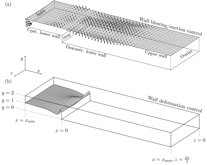
Figure 1: Sketches of steady spanwise-periodic control (wavenumber $\beta$) in a backward facing step: (a) wall blowing/suction applied on the upper wall and (b) wall deformation applied on the upstream lower wall.

Figure 1 shows the optimal spanwise-harmonic control in a BFS of expansion ratio 2. The geometry is bounded by $x\in[-5~{}50]$ and $y\in[0~{}2]$. The spanwise width is fixed at $z=[0~{}2\pi/\beta]$ where $\beta$ is the wavenumber of the control. We aim at optimizing the reattachment location using wall actuation (Fig. 1(a)) or wall deformation (Fig. 1(b)). The Reynolds number is fixed at $Re=500$ throughout the analysis. This ensures that the flow is linearly stable to the steady 3D instability that occurs at $Re=714$ ($Re=748$ with a short inlet channel) with spanwise wavenumber $\beta=0.9$ (Barkley et al., 2002; Lanzerstorfer and Kuhlmann, 2012).

The paper is organized as follows. Section II describes the problem formulation, the general expression of the second-order sensitivity tensor, and the optimization procedure used to compute the optimal control. Section III presents the numerical methods used for the sensitivity analysis and the optimization, as well as for 3D direct numerical simulations dedicated to validation. Global stability properties of the 2D uncontrolled flow are discussed in Sec. IV. The optimal wall actuation and wall deformation for minimizing the lower reattachment location are detailed in Sec. V. We briefly discuss the limitations of the approach in Sec. VI, before concluding in Sec. VII.

II Problem formulation

II.1 Governing equations

Using $h$, $h/U_{in}$ and $\rho h^{3}$ as reference scales for length, time and mass, we consider a steady 2D base flow $\mathbf{Q}(x,y)=(\mathbf{U},P)^{T}(x,y)=(U,V,P)^{T}(x,y)$ in a domain $\Omega$ of boundary $\Gamma$, that satisfies the dimensionless incompressible steady Navier-Stokes equations

$$\boldsymbol{\nabla}\cdot\mathbf{U}=0\quad\mathcal{N}(\mathbf{Q}) =\mathbf{0}\quad\mathrm{in}\ \Omega,$$ (1)

$$\mathbf{U} =\mathbf{0},\quad\mathrm{on}\ \Gamma,$$ (2)

with $\mathcal{N}(\mathbf{Q})\equiv\mathbf{U}\cdot\boldsymbol{\nabla}\mathbf{U}+\boldsymbol{\nabla}P-Re^{-1}\boldsymbol{\nabla}^{2}\mathbf{U}$, and $Re$$=U_{in}h/\nu$ the Reynolds number defined with the maximum incoming velocity $U_{in}$, the step height $h$ and the kinematic viscosity $\nu$.

If there is a recirculation region, with reattachment occurring on a wall defined by $y=y_{w}(x)$, then the reattachment location $x_{r}$ is characterized by vanishing wall shear stress,

$$\left.\frac{\partial U_{t}}{\partial n}\right|_{x=x_{r},y=y_{w}(x_{r})}=0,$$ (3)

i.e. vanishing normal derivative of the tangential velocity. For the sake of simplicity, we now focus on the BFS flow: at the horizontal wall $y=0$, the reattachment location reduces to $\partial_{y}U(x_{r},0)=0$; in addition, the flow separates at the step corner $x_{s}=0$, so the recirculation length $l_{c}=x_{r}-x_{s}$ is simply $l_{c}=x_{r}$.

We assume that a 3D steady control of small amplitude $\epsilon$ is applied on a boundary $\Gamma_{c}$ with actuation velocity $\mathbf{U}_{c}(x,y,z)$, and possibly in the volume with body force $\mathbf{C}(x,y,z)$:

$$\boldsymbol{\nabla}\boldsymbol{\cdot}\mathbf{U}=0,\quad\mathcal{N}(\mathbf{Q}) =\epsilon\mathbf{C}\,\ \quad\mbox{ in }\Omega,$$ (4)

$$\mathbf{U} =\epsilon\mathbf{U}_{c}\quad\mbox{ on }\Gamma_{c},$$ (5)

$$\mathbf{U} =\mathbf{0}\,\qquad\mbox{ on }\Gamma\setminus\Gamma_{c}.$$ (6)

This 3D control modifies the 2D base flow as

$$\mathbf{Q}(x,y,z) =\mathbf{Q}_{0}(x,y) +\epsilon\mathbf{Q}_{1}(x,y,z) +\epsilon^{2}\mathbf{Q}_{2}(x,y,z)+\cdots,$$ (7)

where the $\mathbf{Q}_{i}$ are solutions of the modified base flow equations at orders $\epsilon^{0}$, $\epsilon^{1}$ and $\epsilon^{2}$:

$$\mathcal{N}(\mathbf{Q}_{0}) =\mathbf{0} \quad\mathrm{in}\ \Omega,\quad\mathbf{U}_{0}=\mathbf{0} \quad\mathrm{on}\ \Gamma,$$ (8)

$$\mathbf{A}_{0}\mathbf{Q}_{1} =(\mathbf{C},0)^{T} \quad\mathrm{in}\ \Omega,\quad\mathbf{U}_{1}=\mathbf{U}_{c} \quad\mathrm{on}\ \Gamma_{c},\quad\mathbf{U}_{1}=\mathbf{0}\quad\mathrm{on}\ \Gamma\setminus\Gamma_{c},$$ (9)

$$\mathbf{A}_{0}\mathbf{Q}_{2} =(-\mathbf{U}_{1}\cdot\nabla\mathbf{U}_{1},0)^{T} \quad\mathrm{in}\ \Omega,\quad\mathbf{U}_{2}=\mathbf{0} \quad\mathrm{on}\ \Gamma,$$ (10)

and where $\mathbf{A}_{0}$ is the Navier-Stokes operator linearized about the zeroth-order base flow $\mathbf{Q}_{0}$,

$${\mathbf{A}_{0}} =\left[\begin{array}[]{cccc}\mathbf{U}_{0}\boldsymbol{\cdot}\boldsymbol{\nabla}()+()\boldsymbol{\cdot}\boldsymbol{\nabla}\mathbf{U}_{0}-\mbox{{Re}}^{-1}\boldsymbol{\nabla}^{2}()&\boldsymbol{\nabla}()\\ \boldsymbol{\nabla}\boldsymbol{\cdot}()&0\end{array}\right].$$ (13)

The control and the resulting flow modification alter the reattachment location as

$$x_{r}(z)=x_{r0}+\epsilon x_{r1}(z)+\epsilon^{2}x_{r2}(z)+\cdots.$$ (14)

In this expression, $x_{r0}$ is the reattachment location of the uncontrolled flow $\mathbf{Q}_{0}$,

$$\left.\frac{\partial U_{0}}{\partial y}\right|_{x=x_{r0},y=0}=0.$$ (15)

Similarly, the first-order variation $x_{r1}(z)$ is the reattachment location of the first-order flow modification $\mathbf{Q}_{1}$, characterized implicitly by a vanishing wall shear stress condition,

$$\left.\frac{\partial U_{1}}{\partial y}\right|_{x=x_{r1},y=0,}=0,$$ (16)

and expressed explicitly as (Boujo and Gallaire, 2014b, a, 2015):

$$x_{r1}(z)=-\left.\frac{\partial_{y}U_{1}}{\partial_{xy}U_{0}}\right|_{x=x_{r0},y=0}.$$ (17)

The explicit dependence on $z$ in the notation $x_{r1}(z)$ in (16)-(17) is meant to emphasize that the reattachment line is modulated in the spanwise direction. When the control is harmonic in $z$, as considered in this study, it can actually be shown that $\mathbf{Q}_{1}$ and $x_{r1}$ are purely harmonic too. As a result, the first-order variation $x_{r1}(z)$ has a zero mean. In contrast, the second-order variation $x_{r2}(z)$ has a non-zero mean in general: as detailed in Appendix A, it reads

$$x_{r2}(z) =\left[-\frac{\partial_{y}U_{2}}{\partial_{xy}U_{0}}+\frac{\left(\partial_{y}U_{1}\right)\left(\partial_{xy}U_{1}\right)}{\left(\partial_{xy}U_{0}\right)^{2}}-\frac{\left(\partial_{xxy}U_{0}\right)\left(\partial_{y}U_{1}\right)^{2}}{2\left(\partial_{xy}U_{0}\right)^{3}}\right]_{x=x_{r0},y=0}$$ (18)

$$=x_{r2,\mathrm{I}}+x_{r2,\mathrm{II}}+x_{r2,\mathrm{III}}.$$ (19)

This expression shows that the reattachment location is modified at second order via two effects: $x_{r2,\mathrm{I}}$ depends linearly on the second-order flow modification $\mathbf{Q}_{2}$, and $x_{r2,\mathrm{II}}$ and $x_{r2,\mathrm{III}}$ depend quadratically on the first-order flow modification $\mathbf{Q}_{1}$.

II.2 Sensitivity of the reattachment length: general expression

We introduce the field ${\mathbf{S}}_{\mathrm{I}}$ and the operators ${\mathbf{S}}_{\mathrm{II}}$ and ${\mathbf{S}}_{\mathrm{III}}$ such that the second-order variation $x_{r2}$ can be expressed with scalar products,

$$x_{r2}(z)=\left(\left.{{\mathbf{S}}_{\mathrm{I}}}\,\right|\,{\mathbf{U}_{2}}\right)+\left(\left.{\mathbf{U}_{1}}\,\right|\,{{\mathbf{S}}_{\mathrm{II}}\mathbf{U}_{1}}\right)+\left(\left.{\mathbf{U}_{1}}\,\right|\,{{\mathbf{S}}_{\mathrm{III}}\mathbf{U}_{1}}\right),$$ (20)

where the three terms of the right-hand side correspond to the three terms of (18)-(19), respectively, and $\left(\left.{\cdot}\,\right|\,{\cdot}\right)$ is the Hermitian scalar product in the domain $\Omega$ defined as $\left(\left.{\mathbf{a}}\,\right|\,{\mathbf{b}}\right)\equiv\int_{\Omega}\mathbf{a}^{*}\mathbf{b}\,\mathrm{d}\Omega$, with the superscript ^∗ indicating complex conjugate. For integration along a boundary $\Gamma$, an angled bracket is used: $\left\langle\left.{\mathbf{a}}\,\right|\,{\mathbf{b}}\right\rangle\equiv\int_{\Gamma}\mathbf{a}^{*}\mathbf{b}\,\mathrm{d}\Gamma$. Omitting the notation $y=0$, one identifies from (18)-(19):

$${\mathbf{S}}_{\mathrm{I}} =\dfrac{-1}{\partial_{xy}U_{0}(x_{r0})}\delta(x_{r0})\mathbf{e}_{x}\partial_{y},$$ (21)

$${\mathbf{S}}_{\mathrm{II}} =\dfrac{1}{\left(\partial_{xy}U_{0}(x_{r0})\right)^{2}}\delta(x_{r0})\left(\mathbf{e}_{x}\partial_{y}\right)^{\dagger}\otimes\left(\mathbf{e}_{x}\partial_{xy}\right),$$ (22)

$${\mathbf{S}}_{\mathrm{III}} =\frac{-\partial_{xxy}U_{0}(x_{r0})}{2\left(\partial_{xy}U_{0}(x_{r0})\right)^{3}}\delta(x_{r0})\left(\mathbf{e}_{x}\partial_{y}\right)^{\dagger}\otimes\left(\mathbf{e}_{x}\partial_{y}\right),$$ (23)

where $\delta(x,y)$ is the 2D Dirac delta function, and the superscript ^† denotes the adjoint of an operator defined as $\left(\left.{\mathbf{a}}\,\right|\,{{\mathbf{S}}\mathbf{b}}\right)=\left(\left.{{\mathbf{S}}^{\dagger}\mathbf{a}}\,\right|\,{\mathbf{b}}\right)$. Note that ${\mathbf{S}}_{\mathrm{I}}$, ${\mathbf{S}}_{\mathrm{II}}$ and ${\mathbf{S}}_{\mathrm{III}}$ depend only on $\mathbf{U}_{0}$. From (10), $\mathbf{Q}_{2}$ is uniquely determined by $\mathbf{Q}_{1}$, such that the first term of the right-hand side of (20) can be expressed as

$$x_{r2,\mathrm{I}} =\left(\left.{{\mathbf{S}}_{\mathrm{I}}}\,\right|\,{-\mathbf{A}_{0}^{-1}(\mathbf{U}_{1}\boldsymbol{\cdot}\boldsymbol{\nabla}\mathbf{U}_{1})}\right)=\left(\left.{{\mathbf{A}_{0}^{\dagger}}^{-1}{\mathbf{S}}_{\mathrm{I}}}\,\right|\,{-\mathbf{U}_{1}\boldsymbol{\cdot}\boldsymbol{\nabla}\mathbf{U}_{1}}\right)=\left(\left.{\mathbf{U}^{\dagger}}\,\right|\,{-\mathbf{U}_{1}\boldsymbol{\cdot}\boldsymbol{\nabla}\mathbf{U}_{1}}\right)$$

$$=\left(\left.{\mathbf{U}_{1}}\,\right|\,{{\mathbf{S}}_{\mathrm{I^{\prime}}}\mathbf{U}_{1}}\right),$$ (24)

where we have introduced the 2D adjoint base flow $\mathbf{U}^{\dagger}(x,y)$, defined by

$$\mathbf{A}_{0}^{\dagger}\mathbf{U}^{\dagger}={\mathbf{S}}_{\mathrm{I}},$$ (25)

with $\mathbf{A}_{0}^{\dagger}$ the adjoint Navier-Stokes operator. The adjoint base flow, depicted in Fig. 2, depends only on $\mathbf{U}_{0}$, and is the same adjoint base flow $\mathbf{U}^{\dagger}$ as in Boujo and Gallaire (2014b, 2015) where it represents the first-order sensitivity of the reattachment location $x_{r}$ to a steady 2D volume forcing.

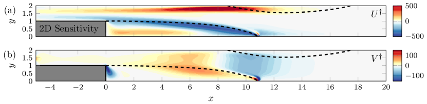
Figure 2: 2D adjoint base flow (a) $U^{\dagger}$ and (b) $V^{\dagger}$. Dashed lines indicate lower and upper recirculation regions, each of them delimited by a wall and a separating streamline (separatrix).

In the last equality of (24), we were allowed to introduce an operator ${\mathbf{S}}_{\mathrm{I^{\prime}}}$ (dependent on $\mathbf{U}^{\dagger}$) because the expression is quadratic in $\mathbf{U}_{1}$. The second-order variation can therefore be expressed quadratically in any flow modification $\mathbf{U}_{1}$ via a single operator for second-order sensitivity to flow modification:

$$x_{r2}(z) =\left(\left.{\mathbf{U}_{1}}\,\right|\,{{\mathbf{S}}_{2,\mathbf{U}_{1}}\mathbf{U}_{1}}\right)\quad\mbox{where}\quad{\mathbf{S}}_{2,\mathbf{U}_{1}}={\mathbf{S}}_{\mathrm{I^{\prime}}}+{\mathbf{S}}_{\mathrm{II}}+{\mathbf{S}}_{\mathrm{III}}.$$ (26)

Finally, using (9), one can introduce operators for the second-order sensitivity to control, dependent only on the uncontrolled flow $\mathbf{U}_{0}$, and such that for any control:

$$x_{r2}(z) =\left(\left.{\mathbf{C}}\,\right|\,{{\mathbf{S}}_{2,\mathbf{C}}\mathbf{C}}\right)+\left\langle\left.{\mathbf{U}_{c}}\,\right|\,{{\mathbf{S}}_{2,\mathbf{U}_{c}}\mathbf{U}_{c}}\right\rangle,$$ (27)

where

$${\mathbf{S}}_{2,\mathbf{C}} =\mathbf{P}^{T}{\mathbf{A}_{0,\mathbf{C}}^{\dagger}}^{-1}{\mathbf{S}}_{2,\mathbf{U}_{1}}{\mathbf{A}_{0,\mathbf{C}}}^{-1}\mathbf{P},$$ (28)

$$\mbox{and }\quad{\mathbf{S}}_{2,\mathbf{U}_{c}} =\mathbf{P}^{T}{\mathbf{A}_{0,\mathbf{U}_{c}}^{\dagger}}^{-1}{\mathbf{S}}_{2,\mathbf{U}_{1}}{\mathbf{A}_{0,\mathbf{U}_{c}}}^{-1}\mathbf{P}.$$ (29)

Here $\mathbf{P}$ is the prolongation matrix that converts the velocity-only space to velocity-pressure space such that $\mathbf{P}\mathbf{U}=(\mathbf{U},0)^{T}$ and $\mathbf{P}^{T}\mathbf{Q}=\mathbf{U}$, and $\mathbf{A}_{0,\mathbf{C}}$ and $\mathbf{A}_{0,\mathbf{U}_{c}}$ are defined by the volume-control-only and wall-control-only versions of (9), respectively:

$$\mathbf{A}_{0,\mathbf{C}}\mathbf{Q}_{1} =(\mathbf{C},0)^{T} \quad\mathrm{in}\ \Omega,\quad\mathbf{U}_{1}=\mathbf{0} \quad\mathrm{on}\ \Gamma,$$ (30)

$$\mathbf{A}_{0,\mathbf{U}_{c}}\mathbf{Q}_{1} =\mathbf{0} \quad\mathrm{in}\ \Omega,\quad\mathbf{U}_{1}=\mathbf{U}_{c} \quad\mathrm{on}\ \Gamma_{c},\quad\mathbf{U}_{1}=\mathbf{0}\quad\mathrm{on}\ \Gamma\setminus\Gamma_{c}.$$ (31)

II.3 Simplification: spanwise-harmonic control

Let us now assume a spanwise-harmonic control of the form

$$\mathbf{U}_{c}(x,y,z)=\left(\begin{array}[]{c}\widetilde{U}_{c}(x,y)\cos(\beta z)\\ \widetilde{V}_{c}(x,y)\cos(\beta z)\\ \widetilde{W}_{c}(x,y)\sin(\beta z)\end{array}\right),\quad\mathbf{C}(x,y,z)=\left(\begin{array}[]{c}\widetilde{C}_{x}(x,y)\cos(\beta z)\\ \widetilde{C}_{y}(x,y)\cos(\beta z)\\ \widetilde{C}_{z}(x,y)\sin(\beta z)\end{array}\right).$$ (32)

The first-order flow modification is also spanwise-harmonic, of same wavenumber $\beta$:

$$\mathbf{Q}_{1}(x,y,z)=\left(\begin{array}[]{c}\widetilde{U}_{1}(x,y)\cos(\beta z)\\ \widetilde{V}_{1}(x,y)\cos(\beta z)\\ \widetilde{W}_{1}(x,y)\sin(\beta z)\\ \widetilde{P}_{1}(x,y)\cos(\beta z)\end{array}\right).$$ (33)

The quadratic term $-\mathbf{U}_{1}\boldsymbol{\cdot}\boldsymbol{\nabla}\mathbf{U}_{1}$ in (10) is then the sum of 2D terms (spanwise-invariant terms, of wavenumber $0$) and 3D terms (of wavenumber $2\beta$), which we denote $\mathbf{f}^{2D}(x,y)+\mathbf{f}^{3D}(x,y,z)$. As a result, the second-order flow modification has the same form: $\mathbf{Q}_{2}^{2D}(x,y)+\mathbf{Q}_{2}^{3D}(x,y,z)$. Similarly, the second and third terms in (18)-(19) and (20) have the same form too, and finally the second-order reattachment location modification reads

$$x_{r2}(z)=x_{r2}^{2D}+x_{r2}^{3D}(z)$$ (34)

where

$$x_{r2}^{2D} =\left[-\frac{\partial_{y}U_{2}^{2D}}{\partial_{xy}U_{0}}+\frac{\left(\partial_{y}\widetilde{U}_{1}\right)\left(\partial_{xy}\widetilde{U}_{1}\right)}{2\left(\partial_{xy}U_{0}\right)^{2}}-\frac{\left(\partial_{xxy}U_{0}\right)\left(\partial_{y}\widetilde{U}_{1}\right)^{2}}{4\left(\partial_{xy}U_{0}\right)^{3}}\right]_{x=x_{r0},y=0}$$ (35)

$$=x_{r2,\mathrm{I}}^{2D}+x_{r2,\mathrm{II}}^{2D}+x_{r2,\mathrm{III}}^{2D}.$$ (36)

Because $x_{r2}^{3D}(z)$ is harmonic of zero mean, we now focus on the spanwise-invariant component $x_{r2}^{2D}$. Its expression can be simplified, taking advantage of the specific form (32) of the control:

$$x_{r2}^{2D} =\left(\left.{\widetilde{\mathbf{C}}}\,\right|\,{\widetilde{\mathbf{S}}_{2,\widetilde{\mathbf{C}}}\widetilde{\mathbf{C}}}\right)+\left\langle\left.{\widetilde{\mathbf{U}}_{c}}\,\right|\,{\widetilde{\mathbf{S}}_{2,\widetilde{\mathbf{U}}_{c}}\widetilde{\mathbf{U}}_{c}}\right\rangle,$$ (37)

where $\widetilde{\mathbf{S}}_{2,\widetilde{\mathbf{C}}}$ and $\widetilde{\mathbf{S}}_{2,\widetilde{\mathbf{U}}_{c}}$ are spanwise-invariant versions of the second-order sensitivity operators (28)-(29) (see detailed expressions in Appendix B). The advantage of this simplification is that calculating the sensitivity operators (and, later, finding the optimal control) can be performed with 2D fields and tensors, rather than 3D ones, which greatly reduces the computational cost and memory requirements.

Figure 3(a) visualizes a 3D flow obtained with spanwise-periodic control. The optimal wall normal blowing/suction control for $\beta=1$ is applied on the upstream part ($x<0$, $y=1$) of the lower wall, with amplitude $\epsilon=0.003$ (see Fig. 8 for the actuation vector). As shown in the sketch of Fig. 3(b), the reattachment location $x_{r}(z)$ is decomposed into zeroth-order $x_{r0}$ (uncontrolled), first-order $x_{r1}(z)$ (of zero mean), and second-order $x_{r2}$. As mentioned earlier, the second-order component is further divided into a zero-mean 3D part $x_{r2}^{3D}(z)$ and a mean 2D part $x_{r2}^{2D}$. Therefore, the spanwise-averaged reattachment location is

$$\overline{x_{r}}=x_{r0}+\epsilon^{2}x_{r2}^{2D},$$ (38)

which is our control interest. The second-order variation $x_{r2}^{2D}$ is now referred to as mean correction.

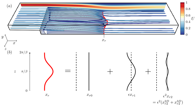
Figure 3: (a) An example of 3D base flow modified by a wall blowing/suction control (using the same control as in Fig. 8 with $\epsilon=0.003$). Streamlines start at $(x,y)=(-5,1.05)$ at different spanwise positions $z$. The iso-surface indicates the lower zero streamwise velocity $U=0$ (the upper recirculation region is not shown here). The thick red line indicates the lower reattachment location characterized by a vanishing wall shear stress $\partial_{y}U=0$. (b) Decomposition of the reattachment location $x_{r}$ into zeroth, first and second-order components $x_{r0}$, $x_{r1}$ and $x_{r2}$. The spanwise-averaged reattachment location is $\overline{x_{r}}=x_{r0}+\epsilon^{2}x_{r2}^{2D}$.

II.4 Optimal spanwise-periodic control

In this section, we show how the spanwise-harmonic control can be optimized so as to yield the largest possible effect on the reattachment location. The formulation is similar to Boujo et al. (2019), where the control was optimized for the largest effect on the linear stability properties (growth rate or frequency, i.e. real or imaginary part of the complex eigenvalue), except that here all quantities are real. We only describe the optimization procedure for boundary control $\widetilde{\mathbf{U}}_{c}$; the derivation for volume control $\widetilde{\mathbf{C}}$ is similar.

II.4.1 Optimal spanwise-periodic wall actuation

If the recirculation length is to be reduced, the mean correction can be minimized by solving the following problem:

$$\min_{||\mathbf{\widetilde{U}_{c}}||=1}\left(x_{r2}^{2D}\right)=\min\frac{\left<\mathbf{\widetilde{U}_{c}}\left|\frac{1}{2}\left(\widetilde{\mathbf{S}}_{2,\widetilde{\mathbf{U}}_{c}}+\widetilde{\mathbf{S}}^{T}_{2,\widetilde{\mathbf{U}}_{c}}\right)\mathbf{\widetilde{U}_{c}}\right.\right>}{\left<\mathbf{\widetilde{U}_{c}}\left|\mathbf{\widetilde{U}_{c}}\right.\right>}=\frac{1}{2}\lambda_{\min}\left(\widetilde{\mathbf{S}}_{2,\widetilde{\mathbf{U}}_{c}}+\widetilde{\mathbf{S}}^{T}_{2,\widetilde{\mathbf{U}}_{c}}\right).$$ (39)

This indicates that, for any given wavenumber $\beta$, the smallest (largest negative) eigenvalue of the symmetric operator $\frac{1}{2}\left(\widetilde{\mathbf{S}}_{2,\widetilde{\mathbf{U}}_{c}}+\widetilde{\mathbf{S}}^{T}_{2,\widetilde{\mathbf{U}}_{c}}\right)$ is the smallest (largest negative) mean correction, and the corresponding eigenvector $\mathbf{U}_{c}$ is the optimal wall control. Similarly, if the recirculation length is to be increased, the mean correction can be maximized by finding the largest positive eigenvalue and the associated eigenvector.

II.4.2 Optimal spanwise-periodic wall deformation

For open-loop control, deforming the geometry can be more interesting than using a steady wall velocity actuation. It is possible to compute the optimal wall deformation, noting that an equivalent wall deformation can be deduced from a given wall blowing/suction control (Boujo et al., 2019). On wall boundaries, the velocity should vanish; for a small-amplitude wall-normal deformation $\epsilon y_{1}$, this condition yields (with a Taylor expansion):

$$\mathbf{U}(y_{0}+\epsilon y_{1}) =\mathbf{U}_{0}(y_{0}+\epsilon y_{1})+\epsilon\mathbf{U}_{1}(y_{0}+\epsilon y_{1})+\cdots$$

$$=\mathbf{U}_{0}(y_{0})+\epsilon\left[y_{1}\partial_{y}\mathbf{U}_{0}(y_{0})+\mathbf{U}_{1}(y_{0})\right]+\cdots=\mathbf{0}.$$ (40)

Noting that $\mathbf{U}_{0}(y_{0})=\mathbf{0}$, this gives the relation between wall-normal deformation $y_{1}$ and equivalent tangential velocity $U_{c}$:

$$U_{1}(y_{0})=-y_{1}\frac{\partial U_{0}(y_{0})}{\partial y}=U_{c}.$$ (41)

Therefore, considering spanwise-harmonic wall-normal deformations of the form

$$y_{1}(z)=\tilde{y}_{1}\cos(\beta z),$$ (42)

the mean correction can now be expressed as

$$x_{r2}^{2D}=\left<\widetilde{U}_{c}|\mathbf{\widetilde{S}}_{2,\widetilde{U}_{c}}\widetilde{U}_{c}\right> =\left<\tilde{y}_{1}\partial_{y}{U}_{0}(y_{0})|\mathbf{\widetilde{S}}_{2,\widetilde{U}_{c}}\partial_{y}{U}_{0}(y_{0})\tilde{y}_{1}\right>$$

$$=\left<\tilde{y}_{1}|\mathbf{M}^{\dagger}\mathbf{\widetilde{S}}_{2,\widetilde{U}_{c}}\mathbf{M}\tilde{y}_{1}\right>=\left<\tilde{y}_{1}|\mathbf{\widetilde{S}}_{2,{\tilde{y}}_{1}}\tilde{y}_{1}\right>,$$ (43)

where $\mathbf{M}$ is a weight matrix accounting for the wall shear stress $\partial_{y}U_{0}(y_{0})$ of the uncontrolled flow. Finally, the optimization for wall-normal deformation reads

$$\min_{||{\tilde{y}_{1}}||=1}\left(x_{r2}^{2D}\right)=\min\frac{\left<\tilde{y}_{1}\left|\frac{1}{2}\left(\widetilde{\mathbf{S}}_{2,\tilde{y}_{1}}+\widetilde{\mathbf{S}}^{T}_{2,\tilde{y}_{1}}\right)\tilde{y}_{1}\right.\right>}{\left<\tilde{y}_{1}\left|\tilde{y}_{1}\right.\right>}=\frac{1}{2}\lambda_{\min}\left(\widetilde{\mathbf{S}}_{2,\tilde{y}_{1}}+\widetilde{\mathbf{S}}^{T}_{2,\tilde{y}_{1}}\right).$$ (44)

III Numerical method

III.1 Linear analysis and optimization

The sensitivity analysis and the optimization are conducted using the method described in (Boujo and Gallaire, 2014b, 2015; Boujo et al., 2019). The problem is discretized with a finite-element method using FreeFem++ (Hecht, 2012) with P2 and P1 Taylor-Hood elements for velocity and pressure, respectively. Mesh points are clustered near the reattachment point, yielding a typical number of elements of $1.6\times 10^{5}$ and $10^{6}$ degrees of freedom. The uncontrolled base flow (8) is obtained with a Newton method. Eigenvalues are solved with a restarted Arnoldi method.

At the inlet ($x=-5$), a Poiseuille flow profile is imposed with maximum velocity $U_{in}=1$, and a stress-free condition is applied at the outlet ($x=50$). At $Re=500$, the reattachment location on the lower wall is $x_{r0}=10.87$ (recall $Re=U_{in}h/\nu$ with $h=1$ the step height and $\nu$ the kinematic viscosity). It is well converged: $x_{r0}=10.88$ on a coarser mesh with $4.5\times 10^{4}$ elements.

III.2 Three-dimensional DNS

Direct numerical simulations (DNS) are also carried out for validation of the optimization method, using the open-source code NEK5000 (Fischer et al., 2008). This parallel code is based on the spectral element method where spatial domain is discretized using hexahedral elements. The unknown parameters are obtained using $N$th-order Lagrange polynomial interpolants, based on the Gauss-Lobatto-Legendre quadrature points in each spectral element with $N\geq 6$. A third order backward differentiation formula (BDF3) is employed for time discretization. For the spatial discretization, the diffusive terms are treated implicitly whereas the convective terms are estimated using a third order explicit extrapolation formula (EXT3). Since the explicit extrapolations of the convective terms in the BDF3-EXT3 scheme enforce a restriction on the time step for iterative stability (Karniadakis et al., 1991), we chose the time step so as to have a Courant number CFL $\approx 0.5$.

The computational domain and the boundary conditions are in accordance with the specifications of the BFS used in the sensitivity analysis. Additionally, we impose periodic boundary conditions in the spanwise direction, where the spanwise width $z\in[0\ 2\pi/\beta]$ captures one wavelength for the purpose of validation. Certain cases employing optimal spanwise modulation required the analysis of a domain with two wavelengths, $z\in[0\ 4\pi/\beta]$. The domain is discretized with a structured multiblock grid consisting of 36200 and 72400 spectral elements for the spanwise widths $2\pi/\beta$ and $4\pi/\beta$, respectively. In both cases, the minimum and maximum distances between the adjacent grid points are $2.4\cdot 10^{-3}$ (near the step corner and the reattachment point) and $2.2\cdot 10^{-1}$ (at the outlet), respectively.

IV Linear stability properties of the 2D uncontrolled base flow

In this section, we investigate the characteristics of the uncontrolled base flow. The BFS flow separates at the step corner and reattaches downstream, thus forming a recirculation region. For the BFS of expansion ratio 2 at $Re=500$, there are two recirculation regions: one on the lower wall developing for $x\in[0\ 10.87]$, and another one on the upper wall for $x\in[8.7\ 17.5]$. In this section, we discuss some linear characteristics of the uncontrolled 2D base flow.

IV.1 Global linear stability

We first investigate the eigenvalues of the system. We assume normal mode perturbations $\mathbf{q}^{\prime}=\widehat{\mathbf{q}}(x,y)\exp(\lambda t+\mathrm{i}\beta_{0}z)$ of small-amplitude, complex eigenvalue $\lambda$, and real spanwise wavenumber $\beta_{0}$. We use the subscript ₀ to denote the eigenmode wavenumber (to be distinguished from the control wavenumber $\beta$). We solve the generalized eigenvalue problem

$$\lambda\widehat{\mathbf{q}}={\widetilde{\mathbf{A}}_{0}}\widehat{\mathbf{q}}$$ (45)

associated with the linearized equation for perturbations around the uncontrolled 2D base flow, with no-slip boundary conditions at the walls.

Leading eigenvalues for $Re=500$ are shown in Fig. 4 as a function of the spanwise wavenumber $\beta_{0}$. For the purpose of later comparison, we plot the inverse of the absolute value of $\lambda$. For all wavenumbers, the leading eigenvalue has a negative growth rate (stable, decaying modes), and zero frequency (steady modes; filled circles) except near $\beta_{0}=0.4-0.5$ (oscillating modes; empty circles). There are two local maxima of $1/|\lambda|$ (least stable modes) near $\beta_{0}=0.1$ and $\beta_{0}=1$, in line with the results of Barkley et al. (2002) for $Re=450$.

Some selected global modes are shown in Fig. 5 for $\beta_{0}=0.1$, $0.5$ and $1$. For $\beta_{0}=0.1$, the mode is localized around $x=10$, near the lower reattachment and upper separation points. For $\beta_{0}=0.5$, the mode is largest farther downstream ($x>10$), while for $\beta_{0}=1$ it is localized in the lower recirculation region $x<10$ .

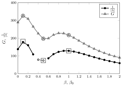
Figure 4: Leading eigenvalue (inverse distance from the origin $1/|\lambda|$) and steady optimal gain $G$, as a function of spanwise wavenumber. Filled circles: steady modes (zero frequency $\lambda_{i}=0$); empty circles: oscillating modes (non-zero frequency). Highlighted wavenumbers: see Figs. 5-6.

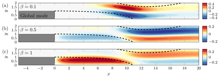
Figure 5: Streamwise velocity of the least stable global eigenmode for (a) $\beta_{0}=0.1$, (b) $\beta_{0}=0.5$ and (c) $\beta_{0}=1$. In (a) and (c) $\hat{u}$ is represented (steady modes) while in (b) the real part $\mbox{Re}({\hat{u}})$ is shown (oscillating mode).

IV.2 Optimal 3D steady forcing

For linearly stable flows, it is interesting to investigate what kind of disturbances undergo the largest amplification. Here we consider in particular a steady spanwise-harmonic forcing $\mathbf{f}=\widehat{\mathbf{f}}(x,y)\exp(\mathrm{i}\beta z)$ acting on the wall boundaries, and resulting linearly in a steady spanwise-periodic response $\mathbf{q}=\widehat{\mathbf{q}}(x,y)\exp(\mathrm{i}\beta z)$ via

$${\widetilde{\mathbf{A}}_{0}}\widehat{\mathbf{q}}=\mathbf{B}_{f}\widehat{\mathbf{f}},$$ (46)

where $\mathbf{B}_{f}$ limits active forcing regions to the walls. The linear amplification efficiency can be measured with a linear gain, for instance as the ratio of the norms of the forcing velocity and response velocity:

$$G=\frac{||\widehat{\mathbf{q}}||}{||\widehat{\mathbf{f}}||}.$$ (47)

This ratio can be maximized: the linear optimal gain is given by the largest singular value of the resolvent operator (here with zero frequency) and the optimal forcing is the associated singular vector Garnaud et al. (2013); Boujo and Gallaire (2015).

The optimal gain for steady wall actuation is shown in Fig. 4 as function of the forcing spanwise wavenumber. The maximum optimal gain $G=326$ is reached for $\beta=0.1$, the same wavenumber as the least stable eigenmode. Qualitatively, the optimal gain varies with the spanwise wavenumber like $1/|\lambda|$ for the leading global mode. This result illustrates the $\varepsilon$-pseudospectral property (Trefethen et al., 1993; Schmid, 2007). Some selected optimal responses are depicted in Fig. 6. As expected, the optimal responses for $\beta=0.1$ and $\beta=1$ are similar to the eigenmodes at the same wavenumbers. For $\beta=0.5$, the optimal response is slightly different from the global mode since the latter has a non-zero frequency while the response is steady.

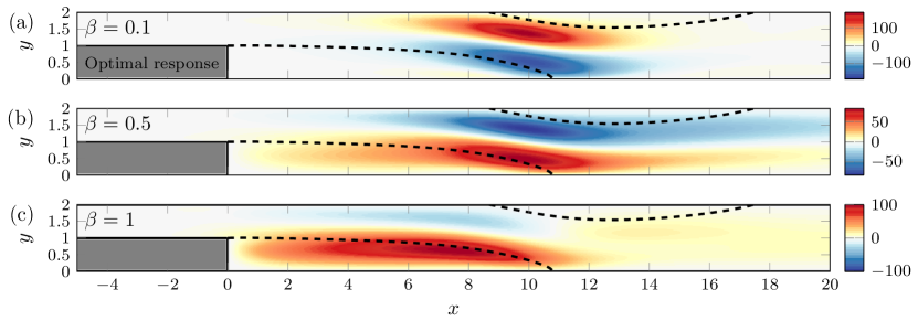
Figure 6: Streamwise velocity (real part $\mbox{Re}({\hat{u}})$) of the optimal response to steady forcing for (a) $\beta=0.1$, (b) $\beta=0.5$ and (c) $\beta=1$.

V Results: optimal control for lower reattachment location

We now turn our attention to the optimal spanwise-harmonic control: wall actuation (blowing/suction) in Sec. V.1, and wall deformation in Sec. V.2. All results are given for $Re=500$.

V.1 Optimal wall actuation

Figure 7(a) shows the optimal negative mean correction $x_{r2}^{2D}$ as a function of $\beta$. Several wall actuation scenarios are considered:

• on the upper wall, with normal velocity $\widetilde{V}_{c}$;

• on the upstream lower wall, with normal velocity $\widetilde{V}_{c}$;

• on the upstream lower wall, with tangential velocity $\widetilde{U}_{c}$.

Recall that 3D velocity controls are defined as $(U_{c},V_{c},W_{c})(x,y,z)=(\widetilde{U}_{c}(x,y)\cos(\beta z),$ $\widetilde{V}_{c}(x,y)\cos(\beta z),\widetilde{W}_{c}(x,y)\sin(\beta z))$. The wall restriction is implemented by modifying the prolongation matrix $\mathbf{P}$.

Wall-normal control $\widetilde{V}_{c}$ is most efficient on the upper wall at $\beta=0.6$, and on the upstream lower wall at $\beta=1$. Wall-tangential actuation $\widetilde{U}_{c}$ on the upstream lower wall has a much smaller effect on the reattachment length than normal actuation. This holds for other types of wall controls (not shown): actuating with normal velocity $\widetilde{V}_{c}$ is generally more efficient than with wall-tangential velocity components $\widetilde{U}_{c}$ and $\widetilde{W}_{c}$.

The individual contributions of terms I, II and III in (36) are shown in Fig. 7(b)-(c) for normal actuation $\widetilde{V}_{c}$ on the upper wall and upstream lower wall, respectively. In both cases, term I (a linear function of the second-order flow modification) contributes the most on the mean correction, while terms II and III (quadratic functions to the first-order flow modification) have negligible or counteracting effects. Control vectors for the upper wall ($\beta=0.6$) and upstream lower wall ($\beta=1$) are shown in Fig. 8. The control is largest near $x=6$ and $x=0$, respectively.

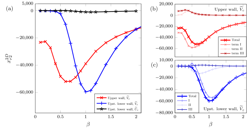
Figure 7: (a) Mean correction $x_{r2}^{2D}$ induced by the optimal wall blowing/suction minimizing the mean reattachment length $\overline{x_{r}}$ (spanwise wavenumber $\beta$, different walls). The individual contributions of the terms I, II and III in (36) (their 2D components) on the total mean correction are detailed in (b) for upper wall, $\widetilde{V}_{c}$ and (c) for upstream lower wall, $\widetilde{V}_{c}$ controls.

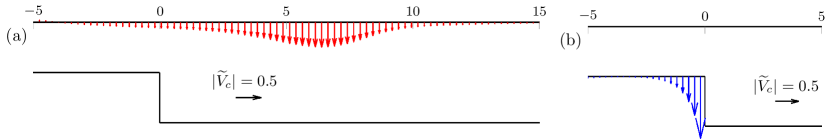
Figure 8: Optimal control $(0,\widetilde{V}_{c},0)$ (a) on the upper wall for $\beta=0.6$ and (b) on the upstream lower wall for $\beta=1$.

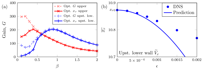
Figure 9: (a) Linear gain $G$ for steady spanwise-periodic wall blowing/suction: control $\widetilde{V}_{c}$ minimizing $x_{r}$ (solid lines) and control $\widehat{\mathbf{f}}$ maximizing $G$ (dashed lines). (b) Mean reattachment location $\overline{x_{r}}$ as a function of the control amplitude for upstream lower wall actuation for $\beta=1$. Line: sensitivity prediction; symbols: 3D DNS.

The linear gain $G$ for these controls is shown in Fig. 9(a) (solid lines). Here the gain is calculated as the ratio between the response $||\widetilde{\mathbf{U}}_{1}||$ and the control $||\widetilde{\mathbf{U}}_{c}||$. The optimal gain obtained when maximizing (47) with wall restriction is also shown in Fig. 9(a) (dashed lines). The gain obtained by maximizing $x_{r2}$ and $G$ itself are close each other, except for lowest $\beta$ values. The corresponding flow modifications $\widetilde{\mathbf{U}}_{1}$ and $\widehat{\mathbf{u}}$ (not shown) are very similar to each other too. This indicates that the amplification potential of the system is closely related to the recirculation length $x_{r}$, as reported in Boujo and Gallaire (2014a).

Figure 9(b) shows the spanwise-averaged reattachment location $\overline{x}_{r}$ computed from 3D DNS along with the sensitivity prediction for the reattachment location $\overline{x}_{r}=x_{0}+\epsilon^{2}x_{r2}^{2D}$ as a function of the actuation amplitude $\epsilon$, for the upstream lower wall case. The agreement is good up to $\epsilon\simeq 0.001$. For this amplitude (equal to 0.1% of the maximum inlet velocity), the optimal control on the upstream lower wall reduces the reattachment location by 0.55%. For larger amplitudes in the investigated range, DNS results start to differ due to strong nonlinear effects, but $\overline{x}_{r}$ continues to decrease.

V.2 Optimal wall deformation

We now investigate the optimal wall deformation for minimizing the lower reattachment point. We focus on the upstream lower wall. The wall deformation is computed using (44), and we apply to $y_{1}$ the smoothing filter $F_{w}=1/(\exp(2C_{k}(x+x_{S}))+1)$, with $C_{k}=250$ and $x_{S}=0.02$, to avoid singularity at the step corner where $\partial_{y}U_{0}$ goes to infinity. This amounts to regularizing the sensitivity (we note that one could also regularize the geometry with a small chamfer at the corner).

Figure 10 shows the effect of the optimal control $x_{r2}^{2D}$ as a function of $\beta$. The most effective spanwise wavenumber is $\beta=1.1$, similar to the wall blowing/suction case, but the efficiency is much lower (minimum $x_{r2}^{2D}$ about 15 times smaller). This is due to the fact that wall deformation is equivalent to a tangential velocity $\widetilde{U}_{c}$, which has a much smaller effect than normal velocity $\widetilde{V}_{c}$ on $x_{r2}$ (recall Fig. 7). Although less effective, wall deformation on the upstream lower wall still results in the mean correction $x_{r2}^{2D}=-3.7\times 10^{3}$.

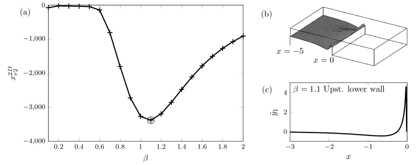
Figure 10: (a) Effect of the optimal upstream lower wall deformation as a function of spanwise wavenumber $\beta$. (b) 3D visualization of the optimal upstream lower wall deformation $y_{1}=\tilde{y}_{1}\cos(\beta z)$ and (c) 2D profile $\tilde{y}_{1}$ for $\beta=1.1$.

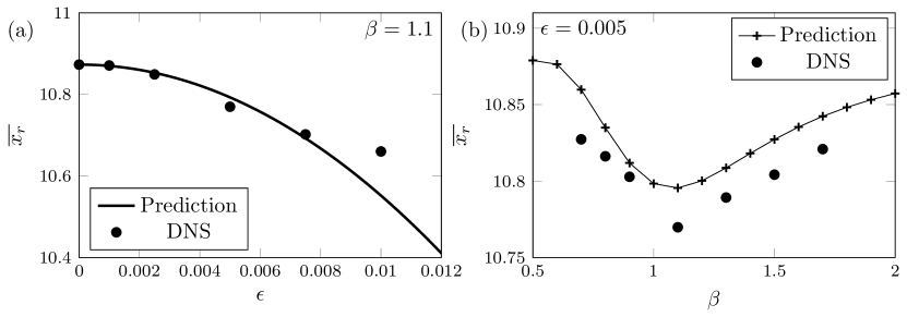
Figure 11: Effect of the optimal wall deformation on the mean reattachment point (a) as a function of $\epsilon$ for fixed $\beta=1.1$ and (b) as a function of $\beta$ for fixed $\epsilon=0.005$.

Figure 10(b)-(c) show the optimal wall deformation $y_{1}$ and its 2D profile $\tilde{y}_{1}$ (recall $y_{1}=\tilde{y}_{1}\cos(\beta z)$). The wall deformation is maximum just before the step corner, where the flow separates. The mean reattachment location from 3D DNS is shown in Fig. 11(a). A good agreement is found until $\epsilon=0.0075$. At this point, $\overline{x}_{r}$ is decreased to $10.7$: a deformation amplitude equal to 0.75% of the inlet channel and step heights reduces the mean reattachment location by 1.5% . For larger deformation amplitudes ($\epsilon>0.01$), DNS results depart from the sensitivity prediction.

Figure 11(b) shows $\overline{x}_{r}$ as a function of $\beta$ for a fixed deformation amplitude $\epsilon=0.005$. Overall, sensitivity predictions and 3D DNS results are in good agreement, with a maximum error $|\overline{x_{r}}_{DNS}-{x}_{r}^{2D}|/\overline{x_{r}}_{DNS}\simeq 0.2\%$ for $\beta=1.1$.

For a larger deformation amplitude $\epsilon=0.015$, the flow becomes unstable. Figure 12 shows an instantaneous flow field with iso-contours of spanwise velocity $W=\pm 0.03$. Because the uncontrolled base flow has no spanwise velocity component, $W$ is a good indicator of velocity perturbations. Those perturbations develop just after the step corner and are sustained in the region $x\in[5\ 40]$. From the top view in Fig. 12(b), clear lines of vanishing $W$ are observed at the nodal points of $\sin(\beta z)$. Chevron patterns appear in the side view in Fig. 12(c). Perturbations oscillate in time at a fundamental frequency $\omega=0.55$ ($St=0.088$). Boujo, Fani and Gallaire Boujo et al. (2015) reported the destabilizing effect of spanwise-periodic control in parallel shear flow. They showed that both fundamental $\beta$ and sub-harmonic $\beta/2$ modes can be excited due to a sub-harmonic resonance mechanism (Herbert, 1988; Hwang et al., 2013). In our DNS with a spanwise domain extended to two control wavelengths ($z\in[0\ 4\pi/\beta]$), and thus able to accommodate perturbations of wavenumber as small as $\beta/2$, perturbations do not show any sub-harmonic component. Instead, only harmonics of $n\beta$ ($n=1,2,3...$) exist, as observed in Fig. 12(b).

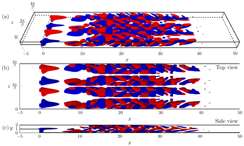
Figure 12: Iso-surfaces of instantaneous spanwise velocity $W=\pm 0.03$ for the optimal wall deformation on the upstream lower, with amplitude $\epsilon=0.015$. (a) oblique view, (b) top view and (c) side view.

VI Discussion

Although the optimization procedure finds the most efficient spanwise-harmonic control, the effect on the mean recirculation length appears relatively small. In light of this observation, it is worth comparing the optimal 2D and 3D blowing/suction. One can show that the optimal 2D wall control is equal to the sensitivity to 2D wall control, given by the adjoint stress at the wall $\left(P^{\dagger}\mathbf{I}+\mbox{{Re}}^{-1}\boldsymbol{\nabla}\mathbf{U}^{\dagger}\right)\mathbf{n}$, where $(\mathbf{U}^{\dagger},P^{\dagger})$ is the adjoint base flow (see Sec. II.2) and $\mathbf{n}$ the outward unit normal vector (Boujo and Gallaire, 2014b, a, 2015). Since the tangential component is generally much smaller than the normal one, we simply consider the sensitivity to 2D normal actuation as the optimal control $(0,V_{c})$.

Figure 13 compares the 3D control optimized on the upstream lower wall ($\beta=1$) to its 2D counterpart, both normalized to 1. The linear response $\boldsymbol{\delta}\mathbf{U}$ to the 2D control is largest and positive near the lower reattachment point, resulting in a positive wall shear stress $\partial_{y}\delta U$ at that location, as expected if $x_{r}$ is to be minimized. Via the spanwise-periodic first-order flow modification $\mathbf{U}_{1}$ (not shown), the optimal 3D control induces a mean second-order flow modification $\mathbf{U}_{2}^{2D}$ that is qualitatively similar to $\boldsymbol{\delta}\mathbf{U}$, resulting in a positive wall shear stress $\partial_{y}U_{2}^{2D}$, and therefore a negative $x_{r2,\mathrm{I}}$ (we do not investigate $x_{r2,\mathrm{II}}$ and $x_{r2,\mathrm{III}}$ since they are much smaller, as shown in Fig. 7). Fig. 14 shows the same quantities optimized on the upper wall ($\beta=0.6$ for the 3D control), and again a qualitatively similar wall shear stress. Although $\mathbf{U}_{2}^{2D}$ is much larger than $\boldsymbol{\delta}\mathbf{U}$, it must be kept in mind that 2D and 3D controls of the same amplitude $\epsilon$ yield a 2D modification that scales linearly ($\sim\epsilon\boldsymbol{\delta}\mathbf{U}$) and a 3D modification that scales quadratically ($\sim\epsilon^{2}\mathbf{U}_{2}^{2D}$), respectively. Spanwise-periodic controls should therefore become more efficient for large enough amplitudes, as previously observed for flow stabilization (Del Guercio et al., 2014a, b, c; Boujo et al., 2015), and as shown in Fig. 15. In practice, when the control amplitude increases, it may happen that the actual efficiency is limited by deviation from the sensitivity prediction (Sec. V.1) or by the flow becoming linearly unstable (Sec. V.2). This can be tested on a case-by-case basis, once promising control candidates have been identified. In this respect, the concept of second-order sensitivity and the associated optimization method allow for a systematic exploration of the best candidates for spanwise-periodic control.

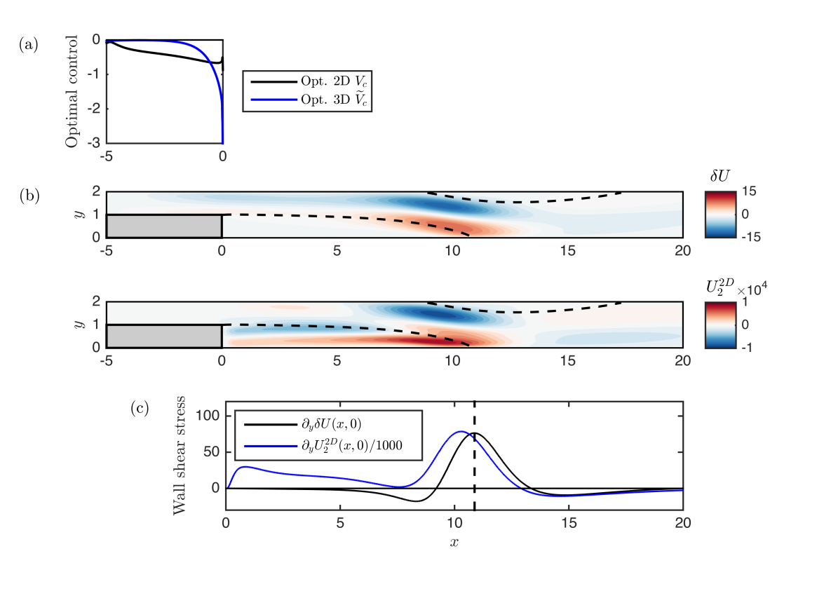
Figure 13: (a) Optimal 2D and 3D ($\beta=1$) vertical controls on the upstream lower wall. (b) Leading-order mean flow modifications (streamwise component). (c) Corresponding wall shear stress on the lower wall.

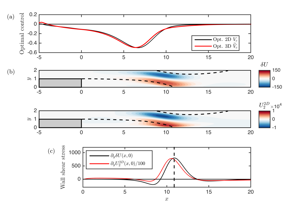
Figure 14: (a) Optimal 2D and 3D ($\beta=0.6$) vertical controls on the upper wall. (b) Leading-order mean flow modifications (streamwise component). (c) Corresponding wall shear stress on the lower wall.

Figure 15: Effect on the reattachment location $x_{r}$ of the optimal vertical 2D control and optimal vertical 3D control ($\beta=1$) of amplitude $\epsilon$, on the upstream lower wall.

This study has focused on $Re=500$. In order to investigate the effect of the Reynolds number, the optimal control has also been computed for other Reynolds numbers up to $Re=700$ (just below the 3D instability threshold). Figure 16(a) shows the second-order variation $x_{r2}^{2D}$ for the optimal vertical blowing/suction $\widetilde{V}_{c}$ on the upstream lower wall. The mean correction reaches a maximum for a peak wavenumber that slightly decreases with $Re$, but remains close to $\beta=1-1.5$. The largest mean correction increases exponentially with $Re$. For instance at $\beta=1$, the mean correction for $Re=700$ ($x_{r0}=12.68$) is $x_{r2}^{2D}=-1.35\cdot 10^{7}$, which is between two and three orders of magnitude larger than for $Re=500$ $(x_{r0}=10.88)$: $x_{r2}^{2D}=-5.95\cdot 10^{4}$. This exponential increase in control authority is similar to the exponential increase in optimal transient growth (Blackburn et al., 2008) and optimal harmonic gain (Boujo and Gallaire, 2015), and can be ascribed to the exponential increase in amplification via a shear mechanism, itself related to the linear increase in recirculation length (e.g. (Barkley et al., 2002)). We note that the profile of the optimal control is very similar at $Re=500$ (Fig. 8b) and $700$ (not shown). Figure 16(b) shows a DNS validation for $Re=700$, $\beta=1$. The effect is indeed much stronger than for $Re=500$ (Fig. 9b) but higher-order effects appear at a smaller control amplitude.

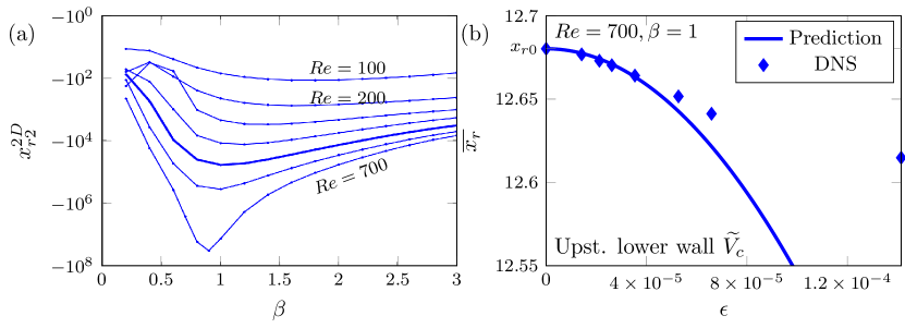
Figure 16: (a) Mean correction $x_{r2}^{2D}$ induced by the optimal wall blowing/suction $\widetilde{V}_{c}$ minimizing the mean reattachment length $\overline{x_{r}}$ (spanwise wavenumber $\beta$, upstream lower wall) for $Re=100,200,...,700$ with the interval $\Delta Re=100$. The thick line indicates $Re=500$. (b) Mean reattachment location $\overline{x_{r}}$ as a function of the control amplitude for upstream lower wall actuation for $\beta=1$ and $Re=700$. Line: sensitivity prediction; symbols: 3D DNS.

VII Conclusion

Initially motivated by the link between recirculation length and stability properties in separated amplifier flows, we have focused on the mean reattachment location as an indicator for the noise amplifying potential in a 3D backward facing step of expansion ratio of 2 and fixed Reynolds number $Re=500$. In this context, our goal was to control the reattachment location on the BFS lower wall with optimal spanwise-periodic control (steady wall blowing/suction or wall deformation) based on the second-order sensitivity analysis introduced by Boujo et al. (2019) for the linear stability properties of the circular cylinder flow.

A second-order sensitivity tensor for the reattachment location has been derived, such that modification of the reattachment location is obtained as a scalar product of this tensor and any arbitrary control. For the specific case of spanwise-harmonic control, the sensitivity tensor was then further simplified, i.e. made independent of $z$. When the control is spanwise harmonic, the first-order reattachment modification takes the same wavenumber with zero mean value, while the second-order modification has a non-zero mean value. Thereby, we have looked for optimal controls that minimize the second-order mean correction.

For wall blowing/suction, we have shown that tangential control has a negligible influence while normal control is the most effective. The optimal wavenumber $\beta$ depends on the control location: $\beta=0.6$ is optimal when controlling on the upper wall, and $\beta=1$ when controlling on the upstream lower wall control. The linear gain for this actuation resembles the optimal gain for 3D steady forcing, indicating that the amplification potential of the BFS is indeed linked to the recirculation length, as also observed in Boujo and Gallaire (2015). Three-dimensional direct numerical simulations have validated the quadratic behaviour of the mean reattachment length modification. The sensitivity prediction is valid until a control amplitude $\epsilon\simeq 0.001$; for larger amplitudes, DNS results start to deviate from the quadratic prediction.

Optimal wall deformation has been studied too. We have focused on deformation of the upstream lower wall, restricting the wall deformation to be null at the step corner. The optimal wall control is generally less effective than wall optimal blowing/suction, and its optimal wavenumber is $\beta=1.1$. DNS validation has shown that the sensitivity prediction is valid until a deformation amplitude $\epsilon\simeq 0.008$; beyond that, the optimal control destabilizes the flow.

Finally, the optimal 3D spanwise-periodic control was compared to the optimal 2D control. The resulting wall shear stress (directly linked to the modification of the reattachment location) is two or three orders of magnitude larger for 3D controls than for 2D ones. Since 2D and 3D controls depend linearly and quadratically on the control amplitude, respectively, the 3D control is more efficient for large enough control amplitudes. In order to determine which of the two controls is best at which amplitude, additional studies are required once the optimal 3D control has been identified. This limitation can be tackled if the mean flow modification is taken into account in the optimization, for instance with a semi-linear approach (Mantič-Lugo et al., 2014; Meliga et al., 2016).

We have not systematically investigated the stability of the controlled flow. Although the spanwise-periodic first-order flow modification does not induce any mean variation of $x_{r}$, it may still alter the flow stability. Clarifying whether this is the case or not would be possible, for a given control, using linear stability analysis (Floquet or 3D global), or non-linear DNS.

Appendix A Appendix: Second-order reattachment location modification

Recall the definition of the reattachment location (Boujo and Gallaire, 2014b, a, 2015):

$$x_{r} =\int_{0}^{\infty}H\left(-\partial_{y}U(x,0)\right)\,\mathrm{d}x,$$ (48)

where $H$ is the Heaviside function such that $H(\theta<0)=0$ and $H(\theta>0)=1$. This expression yields indeed the reattachment location since the wall shear stress $\partial_{y}U(x,0)$ is negative in the recirculation region. Hereafter, we omit $y=0$ for brevity. Substituting

$$U=U_{0}+\epsilon U_{1}+\epsilon^{2}U_{2}+O\left(\epsilon^{3}\right)$$ (49)

into (48), one obtains:

$$x_{r} =\int_{0}^{\infty}H\left[-\partial_{y}U_{0}-\epsilon\partial_{y}U_{1}-\epsilon^{2}\partial_{y}U_{2}+O\left(\epsilon^{3}\right)\right]\,\mathrm{d}x$$

$$=\int_{0}^{\infty}\left\{H\left(-\partial_{y}U_{0}\right)-\left[\epsilon\partial_{y}U_{1}+\epsilon^{2}\partial_{y}U_{2}+O\left(\epsilon^{3}\right)\right]H^{\prime}\left(-\partial_{y}U_{0}\right)+\frac{1}{2}\left[\epsilon\partial_{y}U_{1}+O\left(\epsilon^{2}\right)\right]^{2}H^{\prime\prime}\left(-\partial_{y}U_{0}\right)\right\}\,\mathrm{d}x$$

$$=\int_{0}^{\infty}H\left(-\partial_{y}U_{0}\right)\,\mathrm{d}x$$

$$\quad-\epsilon\int_{0}^{\infty}\left(\partial_{y}U_{1}\right)H^{\prime}\left(-\partial_{y}U_{0}\right)\,\mathrm{d}x$$

$$\quad+\epsilon^{2}\int_{0}^{\infty}\left\{\left(-\partial_{y}U_{2}\right)H^{\prime}\left(-\partial_{y}U_{0}\right)+\frac{1}{2}\left(\partial_{y}U_{1}\right)^{2}H^{\prime\prime}\left(-\partial_{y}U_{0}\right)\right\}\,\mathrm{d}x+O\left(\epsilon^{3}\right).$$ (50)

The zeroth-order term is the reattachment location $x_{r0}$ of the uncontrolled flow. The first-order term $x_{r1}$ is linear in $U_{1}$ and is therefore zero when averaging over $z$. The second-order term contains derivatives of $H$, that can be obtained defining $G(x)=H\left(-\partial_{y}U(x,0)\right)=H(\theta)$ and using the relations

$$G^{\prime}(x) =\frac{\mathrm{d}{\left(H(\theta)\right)}}{\mathrm{d}{x}}=\frac{\mathrm{d}{H}}{\mathrm{d}{\theta}}\frac{\mathrm{d}{\theta}}{\mathrm{d}{x}}=-H^{\prime}(\theta)\partial_{xy}U,$$ (51)

$$G^{\prime\prime}(x) =\frac{\mathrm{d}{}}{\mathrm{d}{x}}\left(-H^{\prime}(\theta)\partial_{xy}U\right)$$

$$=-H^{\prime}(\theta)\frac{\mathrm{d}{}}{\mathrm{d}{x}}\left(\partial_{xy}U\right)-\frac{\mathrm{d}{\left(H^{\prime}(\theta)\right)}}{\mathrm{d}{x}}\partial_{xy}U$$

$$=-H^{\prime}(\theta)\partial_{xxy}U-\frac{\mathrm{d}{{}^{2}H}}{\mathrm{d}{\theta}}\frac{\mathrm{d}{\theta}}{\mathrm{d}{x}}\partial_{xy}U$$

$$=-H^{\prime}(\theta)\partial_{xxy}U+H^{\prime\prime}(\theta)\left(\partial_{xy}U\right)^{2},$$ (52)

which yields

$$H^{\prime}(\theta) =-\frac{G^{\prime}(x)}{\partial_{xy}U}=\frac{\delta(x-x_{r})}{\partial_{xy}U},$$ (53)

$$H^{\prime\prime}(\theta) =\frac{1}{\left(\partial_{xy}U\right)^{2}}\left(H^{\prime}(\theta)\partial_{xxy}U+G^{\prime\prime}(x)\right)=\frac{1}{\left(\partial_{xy}U\right)^{2}}\left(\frac{\delta(x-x_{r})}{\partial_{xy}U}\partial_{xxy}U-\delta^{\prime}(x-x_{r})\right),$$ (54)

with $\delta(x)$ the Dirac delta function. The second-order term thus becomes:

$$x_{r2} =\int_{0}^{\infty}\left\{\left(-\partial_{y}U_{2}\right)H^{\prime}(\theta_{0})+\frac{1}{2}\left(\partial_{y}U_{1}\right)^{2}H^{\prime\prime}(\theta_{0})\right\}\,\mathrm{d}x$$

$$=\int_{0}^{\infty}\left\{\left(-\partial_{y}U_{2}\right)\frac{\delta(x-x_{r})}{\partial_{xy}U_{0}}+\frac{1}{2}\frac{\left(\partial_{y}U_{1}\right)^{2}}{\left(\partial_{xy}U_{0}\right)^{2}}\left(\frac{\delta(x-x_{r})}{\partial_{xy}U_{0}}\partial_{xxy}U_{0}-\delta^{\prime}(x-x_{r})\right)\right\}\,\mathrm{d}x$$

$$=-\frac{\partial_{y}U_{2}(x_{r0})}{\partial_{xy}U_{0}(x_{r0})}+\left.\frac{1}{2}\frac{\left(\partial_{y}U_{1}\right)^{2}}{\left(\partial_{xy}U_{0}\right)^{2}}\frac{\partial_{xxy}U_{0}}{\partial_{xy}U_{0}}\right|_{x_{r0}}+\frac{1}{2}\frac{\mathrm{d}{}}{\mathrm{d}{x}}\left[\frac{\left(\partial_{y}U_{1}\right)^{2}}{\left(\partial_{xy}U_{0})\right)^{2}}\right]_{x_{r0}}$$

$$=\left.-\frac{\partial_{y}U_{2}}{\partial_{xy}U_{0}}\right|_{x_{r0}}+\left.\frac{\left(\partial_{y}U_{1}\right)\left(\partial_{xy}U_{1}\right)}{\left(\partial_{xy}U_{0}\right)^{2}}\right|_{x_{r0}}-\left.\frac{\left(\partial_{xxy}U_{0}\right)\left(\partial_{y}U_{1}\right)^{2}}{2\left(\partial_{xy}U_{0}\right)^{3}}\right|_{x_{r0}}.$$ (55)

Appendix B Appendix: Simplification of the sensitivity operators

With a spanwise-periodic control of the form

$$\mathbf{U}_{c}(x,y,z)=\left(\begin{array}[]{c}\widetilde{U}_{c}(x,y)\cos(\beta z)\\ \widetilde{V}_{c}(x,y)\cos(\beta z)\\ \widetilde{W}_{c}(x,y)\sin(\beta z)\end{array}\right),\quad\mathbf{C}(x,y,z)=\left(\begin{array}[]{c}\widetilde{C}_{x}(x,y)\cos(\beta z)\\ \widetilde{C}_{y}(x,y)\cos(\beta z)\\ \widetilde{C}_{z}(x,y)\sin(\beta z)\end{array}\right),$$ (56)

the 1st-order flow modification is of the form

$$\mathbf{Q}_{1}(x,y,z)=\left(\begin{array}[]{c}\widetilde{U}_{1}(x,y)\cos(\beta z)\\ \widetilde{V}_{1}(x,y)\cos(\beta z)\\ \widetilde{W}_{1}(x,y)\sin(\beta z)\\ \widetilde{P}_{1}(x,y)\cos(\beta z)\end{array}\right).$$ (57)

Let us consider the first term $x_{r2,\mathrm{I}}$ in (18)-(20). Given the form of $\mathbf{Q}_{1}$, the right-hand side $-\mathbf{U}_{1}\boldsymbol{\cdot}\boldsymbol{\nabla}\mathbf{U}_{1}$ of (10) is the sum of 2D and 3D terms:

$$\mathbf{f}^{2D}(x,y) =-\frac{1}{2}\left(\begin{array}[]{c}(\widetilde{U}_{1}{\partial}_{x}+\widetilde{V}_{1}{\partial}_{y}-\beta\widetilde{W}_{1})\widetilde{U}_{1}\\ (\widetilde{U}_{1}{\partial}_{x}+\widetilde{V}_{1}{\partial}_{y}-\beta\widetilde{W}_{1})\widetilde{V}_{1}\\ 0\end{array}\right),$$ (61)

$$\mathbf{f}^{3D}(x,y,z) =-\frac{1}{2}\left(\begin{array}[]{c}(\widetilde{U}_{1}{\partial}_{x}+\widetilde{V}_{1}{\partial}_{y}+\beta\widetilde{W}_{1})\widetilde{U}_{1}\cos(2\beta z)\\ (\widetilde{U}_{1}{\partial}_{x}+\widetilde{V}_{1}{\partial}_{y}+\beta\widetilde{W}_{1})\widetilde{V}_{1}\cos(2\beta z)\\ (\widetilde{U}_{1}{\partial}_{x}+\widetilde{V}_{1}{\partial}_{y}+\beta\widetilde{W}_{1})\widetilde{W}_{1}\sin(2\beta z)\end{array}\right).$$ (65)

The spanwise-harmonic forcing $\mathbf{f}^{3D}(x,y,z)$ induces a 3D spanwise-harmonic response $\mathbf{Q}_{2}^{3D}(x,y,z)$ that yields a zero-mean variation $x_{r2,\mathrm{I}}^{3D}(z)$. By contrast, the 2D forcing term $\mathbf{f}^{2D}(x,y)$ induces the 2D response

$$\mathbf{Q}_{2}^{2D}(x,y)=\left(\begin{array}[]{c}U_{2}^{2D}(x,y)\\ V_{2}^{2D}(x,y)\\ 0\\ P_{2}^{2D}(x,y)\end{array}\right)$$ (66)

that yields a non-zero mean $x_{r2,\mathrm{I}}^{2D}$. Recalling (24), one can therefore write

$$x_{r2,\mathrm{I}}^{2D} =\left(\left.{\mathbf{U}^{\dagger}}\,\right|\,{\mathbf{f}^{2D}}\right)$$ (67)

$$=-\dfrac{1}{2}\iint U^{\dagger}(\widetilde{U}_{1}{\partial}_{x}+\widetilde{V}_{1}{\partial}_{y}-\beta\widetilde{W}_{1})\widetilde{U}_{1}+V^{\dagger}(\widetilde{U}_{1}{\partial}_{x}+\widetilde{V}_{1}{\partial}_{y}-\beta\widetilde{W}_{1})\widetilde{V}_{1}$$ (68)

$$=-\dfrac{1}{2}\iint\widetilde{U}_{1}(U^{\dagger}{\partial}_{x}\widetilde{U}_{1}+V^{\dagger}{\partial}_{x}\widetilde{V}_{1}-\beta\widetilde{W}_{1}U^{\dagger})+\widetilde{V}_{1}(U^{\dagger}{\partial}_{y}\widetilde{U}_{1}+V^{\dagger}{\partial}_{y}\widetilde{V}_{1}-\beta\widetilde{W}_{1}V^{\dagger})$$ (69)

$$=\left(\left.{\widetilde{\mathbf{U}}_{1}}\,\right|\,{\widetilde{\mathbf{S}}_{\mathrm{I}^{\prime}}\widetilde{\mathbf{U}}_{1}}\right),$$ (70)

where the simplified second-order sensitivity operator

$$\widetilde{\mathbf{S}}_{\mathrm{I}^{\prime}}=-\frac{1}{2}\left[\begin{array}[]{ccc}U^{\dagger}\partial_{x}&V^{\dagger}\partial_{x}&0\\ U^{\dagger}\partial_{y}&V^{\dagger}\partial_{y}&0\\ -\beta U^{\dagger}&-\beta V^{\dagger}&0\end{array}\right]$$ (74)

can be seen formally as a 2D restriction of the operator $\mathbf{U}^{\dagger}\boldsymbol{\cdot}\boldsymbol{\nabla}()^{T}$.

Let us now consider the second and third terms $x_{r2,\mathrm{II}}$ and $x_{r2,\mathrm{III}}$ in (18)-(20). Given (57), it is straightforward to show that

$$x_{r2,\mathrm{II}}^{2D}=\left(\left.{\widetilde{\mathbf{U}}_{1}}\,\right|\,{\widetilde{\mathbf{S}}_{\mathrm{II}}\widetilde{\mathbf{U}}_{1}}\right),\qquad x_{r2,\mathrm{III}}^{2D}=\left(\left.{\widetilde{\mathbf{U}}_{1}}\,\right|\,{\widetilde{\mathbf{S}}_{\mathrm{III}}\widetilde{\mathbf{U}}_{1}}\right),$$ (75)

where the simplified second-order sensitivity operators are

$$\widetilde{\mathbf{S}}_{\mathrm{II}} =\dfrac{1}{2\left(\partial_{xy}U_{0}(x_{r0})\right)^{2}}\delta(x_{r0})\left(\mathbf{e}_{x}\partial_{y}\right)^{\dagger}\otimes\left(\mathbf{e}_{x}\partial_{xy}\right),$$ (76)

$$\widetilde{\mathbf{S}}_{\mathrm{III}} =\frac{-\partial_{xxy}U_{0}(x_{r0})}{4\left(\partial_{xy}U_{0}(x_{r0})\right)^{3}}\delta(x_{r0})\left(\mathbf{e}_{x}\partial_{y}\right)^{\dagger}\otimes\left(\mathbf{e}_{x}\partial_{y}\right),$$ (77)

Finally, the mean second-order variation is

$$x_{r2}^{2D} =\left(\left.{\widetilde{\mathbf{U}}_{1}}\,\right|\,{\widetilde{\mathbf{S}}_{2,\widetilde{\mathbf{U}}_{1}}\widetilde{\mathbf{U}}_{1}}\right)\quad\mbox{where}\quad\widetilde{\mathbf{S}}_{2,\widetilde{\mathbf{U}}_{1}}=\widetilde{\mathbf{S}}_{\mathrm{I^{\prime}}}+\widetilde{\mathbf{S}}_{\mathrm{II}}+\widetilde{\mathbf{S}}_{\mathrm{III}},$$ (78)

and the second-order sensitivities to control defined by (37) read

$$\widetilde{\mathbf{S}}_{2,\widetilde{\mathbf{C}}} =\mathbf{P}^{T}\left.{\widetilde{\mathbf{A}}_{0,\widetilde{\mathbf{C}}}}^{\dagger}\right.^{-1}\widetilde{\mathbf{S}}_{2,\widetilde{\mathbf{U}}_{1}}\left.{\widetilde{\mathbf{A}}_{0,\widetilde{\mathbf{C}}}}\right.^{-1}\mathbf{P}\quad(\mbox{volume-forcing-only }{\widetilde{\mathbf{A}}_{0,\widetilde{\mathbf{C}}}}),$$ (79)

$$\widetilde{\mathbf{S}}_{2,\widetilde{\mathbf{U}}_{c}} =\mathbf{P}^{T}\left.{\widetilde{\mathbf{A}}_{0,\widetilde{\mathbf{U}}_{c}}}^{\dagger}\right.^{-1}\widetilde{\mathbf{S}}_{2,\widetilde{\mathbf{U}}_{1}}\left.{\widetilde{\mathbf{A}}_{0,\widetilde{\mathbf{U}}_{c}}}\right.^{-1}\mathbf{P}\quad(\mbox{wall-forcing-only }{\widetilde{\mathbf{A}}_{0,\widetilde{\mathbf{U}}_{c}}}),$$ (80)

with

$${\widetilde{\mathbf{A}}_{0}}=\left[\begin{array}[]{cccc}U_{0}{\partial}_{x}+V_{0}{\partial}_{y}+{\partial}_{x}U_{0}-\widetilde{D}&{\partial}_{y}U_{0}&0&{\partial}_{x}\\ {\partial}_{x}V_{0}&U_{0}{\partial}_{x}+V_{0}{\partial}_{y}+{\partial}_{y}V_{0}-\widetilde{D}&0&{\partial}_{y}\\ 0&0&U_{0}{\partial}_{x}+V_{0}{\partial}_{y}-\widetilde{D}&-\beta\\ {\partial}_{x}&{\partial}_{y}&\beta&0\end{array}\right],$$ (85)

$$\widetilde{D}=\mbox{{Re}}^{-1}({\partial}_{xx}+{\partial}_{yy}-\beta^{2}).$$ (86)

References

- Lanzerstorfer and Kuhlmann (2012) D. Lanzerstorfer and H. Kuhlmann, “Global stability of the two-dimensional flow over a backward-facing step,” J. Fluid Mech. 693, 1–27 (2012).
- Barkley et al. (2002) D. Barkley, M. G. M. Gomes, and R. D. Henderson, “Three-dimensional instability in flow over a backward-facing step,” J. Fluid Mech. 473, 167–190 (2002).
- Marquet and Sipp (2010) O. Marquet and D. Sipp, “Global sustained perturbations in a backward-facing step flow,” in Seventh IUTAM Symposium on Laminar-Turbulent Transition (Springer Netherlands, Dordrecht, 2010) pp. 525–528.
- Blackburn et al. (2008) H. M. Blackburn, D. Barkley, and S. J. Sherwin, “Convective instability and transient growth in flow over a backward-facing step,” J. Fluid Mech. 603, 271–304 (2008).
- Boujo and Gallaire (2015) E. Boujo and F. Gallaire, “Sensitivity and open-loop control of stochastic response in a noise amplifier flow: the backward-facing step,” J. Fluid Mech. 762, 361–392 (2015).
- McManus et al. (1990) K. R. McManus, U. Vandsburger, and C. T. Bowman, “Combustor performance enhancement through direct shear layer excitation,” Combust. Flame. 82, 75–92 (1990).
- McManus and Bowman (1991) K. R. McManus and C. T. Bowman, “Effects of controlling vortex dynamics on the performance of a dump combustor,” in Proc. Combust. Inst., Vol. 23 (Elsevier, 1991) pp. 1093–1099.
- Ghoniem et al. (2002) A. F. Ghoniem, A. Annaswamy, D. Wee, T. Yi, and S. Park, “Shear flow-driven combustion instability: Evidence, simulation, and modeling,” Proc. Combust. Inst. 29, 53–60 (2002).
- Pujals et al. (2011) G Pujals, S Depardon, and C Cossu, “Transient growth of coherent streaks for control of turbulent flow separation,” Int. J. Aerodyn. 1, 318–336 (2011).
- Tanner (1972) M Tanner, “A method for reducing the base drag of wings with blunt trailing edge,” Aeronautical Quarterly 23, 15–23 (1972).
- Zdravkovich (1981) M.M. Zdravkovich, “Review and classification of various aerodynamic and hydrodynamic means for suppressing vortex shedding,” J. Wind Eng. Ind. Aerod. 7, 145–189 (1981).
- Tombazis and Bearman (1997) N. Tombazis and P.W. Bearman, “A study of three-dimensional aspects of vortex shedding from a bluff body with a mild geometric disturbance,” J. Fluids Struct. 330, 85–112 (1997).
- Bearman and Owen (1998) P.W. Bearman and J.C. Owen, “Reduction of bluff-body drag and suppression of vortex shedding by the introduction of wavy separation lines,” J. Fluid Mech. 12, 123–130 (1998).
- Choi et al. (2008) H. Choi, W.-P. Jeon, and J. Kim, “Control of flow over a bluff body,” Annu. Rev. Fluid Mech. 40, 113–139 (2008).
- Ahmed and Bays-Muchmore (1992) A. Ahmed and B. Bays-Muchmore, “Transverse flow over a wavy cylinder,” Phys. Fluids A 4, 1959–1967 (1992).
- Ahmed et al. (1993) A. Ahmed, M.J. Khan, and B. Bays-Muchmore, “Experimental investigation of a three-dimensional bluff-body wake,” AIAA 31, 559–563 (1993).
- Lee and Nguyen (2007) S.-J. Lee and A.-T. Nguyen, “Experimental investigation on wake behind a wavy cylinder having sinusoidal cross-sectional area variation,” Fluid Dyn. Res. 39, 292 (2007).
- Lam and Lin (2008) K. Lam and Y.F. Lin, “Large eddy simulation of flow around wavy cylinders at a subcritical reynolds number,” Int. J. Heat Fluid Fl. 29, 1071–1088 (2008).
- Zhang et al. (2016) K. Zhang, H. Katsuchi, D. Zhou, H. Yamada, and Z. Han, “Numerical study on the effect of shape modification to the flow around circular cylinders,” J. Wind Eng. Ind. Aerod. 152, 23–40 (2016).
- Lam et al. (2012) K. Lam, Y.F. Lin, and Y. Zou, L .and Liu, “Numerical study of flow patterns and force characteristics for square and rectangular cylinders with wavy surfaces,” J. Fluids Struct. 28, 359–377 (2012).
- Lin et al. (2013) Y.F. Lin, K. Lam, L. Zou, and Y. Liu, “Numerical study of flows past airfoils with wavy surfaces,” J. Fluids Struct. 36, 136–148 (2013).
- Serson et al. (2017) D. Serson, J.R. Meneghini, and S.J. Sherwin, “Direct numerical simulations of the flow around wings with spanwise waviness,” J. Fluid Mech. 826, 714–731 (2017).
- Hill (1992) D.C. Hill, “A theoretical approach for analyzing the restabilization of wakes,” in AIAA (1992) pp. 92–0067.
- Marquet et al. (2008) O. Marquet, D. Sipp, and L. Jacquin, “Sensitivity analysis and passive control of cylinder flow,” J. Fluid Mech. 615, 221–252 (2008).
- Hinch (1991) E.J. Hinch, Perturbation Methods (Cambridge University Press, 1991).
- Cossu (2014) C. Cossu, “On the stabilizing mechanism of 2D absolute and global instabilities by 3D streaks,” arXiv preprint arXiv:1404.3191 (2014).
- Boujo et al. (2015) E. Boujo, A. Fani, and F. Gallaire, “Second-order sensitivity of parallel shear flows and optimal spanwise-periodic flow modifications,” J. Fluid Mech. 782, 491–514 (2015).
- Hwang et al. (2013) Y. Hwang, J. Kim, and H. Choi, “Stabilization of absolute instability in spanwise wavy two-dimensional wakes,” J. Fluid Mech. 727, 346–378 (2013).
- Del Guercio et al. (2014a) G. Del Guercio, C. Cossu, and G. Pujals, “Optimal perturbations of non-parallel wakes and their stabilizing effect on the global instability,” Phys. Fluids 26, 024110 (2014a).
- Del Guercio et al. (2014b) G. Del Guercio, C. Cossu, and G. Pujals, “Optimal streaks in the circular cylinder wake and suppression of the global instability,” J. Fluid Mech. 752, 572–588 (2014b).
- Del Guercio et al. (2014c) G. Del Guercio, C. Cossu, and G. Pujals, “Stabilizing effect of optimally amplified streaks in parallel wakes,” J. Fluid Mech. 739, 37–56 (2014c).
- Tammisola et al. (2014) O. Tammisola, F. Giannetti, V. Citro, and M.P. Juniper, “Second-order perturbation of global modes and implications for spanwise wavy actuation,” J. Fluid Mech. 755, 314–335 (2014).
- Sinha et al. (1981) S.N. Sinha, A.K. Gupta, and M. Oberai, “Laminar separating flow over backsteps and cavities. Part I: Backsteps,” AIAA 19, 1527–1530 (1981).
- Armaly et al. (1983) B. F. Armaly, F. Durst, J.C.F. Pereira, and B. Schönung, “Experimental and theoretical investigation of backward-facing step flow,” J. Fluid Mech. 127, 473–496 (1983).
- Boujo and Gallaire (2014a) E. Boujo and F. Gallaire, “Manipulating flow separation: sensitivity of stagnation points, separatrix angles and recirculation area to steady actuation,” Proc. Roy. Soc. Lond. A 470, 20140365 (2014a).
- Boujo et al. (2019) E. Boujo, A. Fani, and F. Gallaire, “Second-order sensitivity in the cylinder wake: Optimal spanwise-periodic wall actuation and wall deformation,” Phys. Rev. Fluids 4, 053901 (2019).
- Boujo and Gallaire (2014b) E. Boujo and F. Gallaire, “Controlled reattachment in separated flows: a variational approach to recirculation length reduction,” J. Fluid Mech. 742, 618–635 (2014b).
- Hecht (2012) F. Hecht, “New development in freefem++,” J. Numer. Math. 20, 251–265 (2012).
- Fischer et al. (2008) P. F. Fischer, J. W. Lottes, and S. G. Kerkemeier, “Nek5000 Web page,” (2008), http://nek5000.mcs.anl.gov.
- Karniadakis et al. (1991) G. E. Karniadakis, M. Israeli, and S. A. Orszag, “High-order splitting methods for the incompressible navier-stokes equations,” J. Comp. Phys. 97, 414–443 (1991).
- Garnaud et al. (2013) X. Garnaud, L. Lesshafft, P. J. Schmid, and P. Huerre, “The preferred mode of incompressible jets: linear frequency response analysis,” J. Fluid Mech. 716, 189–202 (2013).
- Trefethen et al. (1993) L. N. Trefethen, A. E. Trefethen, S. C. Reddy, and T. A. Driscoll, “Hydrodynamic stability without eigenvalues,” Science 261, 578–584 (1993).
- Schmid (2007) P. J. Schmid, “Nonmodal stability theory,” Annu. Rev. Fluid Mech. 39, 129–162 (2007).
- Herbert (1988) T. Herbert, “Secondary instability of boundary layers,” Annu. Rev. Fluid Mech. 20, 487–526 (1988).
- Mantič-Lugo et al. (2014) V. Mantič-Lugo, C., C. Arratia, and F. Gallaire, “Self-consistent mean flow description of the nonlinear saturation of the vortex shedding in the cylinder wake,” Phys. Rev. Lett. 113, 084501 (2014).
- Meliga et al. (2016) P. Meliga, E. Boujo, and F. Gallaire, “A self-consistent formulation for the sensitivity analysis of finite-amplitude vortex shedding in the cylinder wake,” J. Fluid Mech. 800, 327–357 (2016).