Reduced Order Estimation of the Speckle Electric Field History for Space-Based Coronagraphs

Abstract

In high-contrast space-based coronagraphs, one of the main limiting factors for imaging the dimmest exoplanets is the time varying nature of the residual starlight (speckles). Modern methods try to differentiate between the intensities of starlight and other sources, but none incorporate models of space-based systems which can take into account actuations of the deformable mirrors. Instead, we propose formulating the estimation problem in terms of the electric field while allowing for dithering of the deformable mirrors. Our reduced-order approach is similar to intensity-based PCA (e.g. KLIP) although, under certain assumptions, it requires a considerably lower number of modes of the electric field. We illustrate this by a FALCO simulation of the WFIRST hybrid Lyot coronagraph.

1 Introduction

Direct imaging of exoplanets and circumstellar disks requires an observatory that creates a high contrast between the astrophysical source and the residual starlight halo (speckles). The contrast needed to detect and characterize Earth-like planets is on the order of $10^{10}$ and can be achieved only by going to space to avoid the fundamental limitations imposed by atmospheric turbulence (Guyon (2005); Cavarroc et al. (2006)). The Coronagraph Instrument (CGI) on NASA’s upcoming Wide-Field Infra-Red Survey Telescope (WFIRST) is designed to demonstrate the viability of such missions (Douglas et al. (2018)). It will employ passive and active starlight suppression systems (coronagraphs, deformable mirrors, etc.) to block most of the starlight and control the diffraction pattern in a region of the image where the planet is located (Demers et al. (2015); Demers (2018)). Yet, the speckle background is expected to remain brighter than the planet and to vary over the lengthy observation time (Shaklan et al. (2011); Ygouf et al. (2016)). It is therefore necessary to post-process the images to distinguish between the speckles and the signals incoherent with the star (which include the planet). We will refer to the ratio between the intensity of the speckle floor and the dimmest detectable planet as the post-processing factor.

Post-processing methods for ground based telescopes exploit various sources of diversity between images to extract the faint signal from the varying background (for a review, see Pueyo (2018); Jovanovic et al. (2018)). Some utilize physical properties such as the rotation of the telescope (Marois et al. (2006)), phase apodization (Codona et al. (2006); Kenworthy et al. (2007)), the spectrum of the planet and the star (Marois et al. (2000); Sparks & Ford (2002); Martinache (2010)), and their polarization (Baba & Murakami (2003)). Others rely on mathematical manipulations of multiple images, either only from the target star (Lafreniere et al. (2007)), or from additional observations of reference stars (Mawet et al. (2012)), and even artificial speckles (Jovanovic et al. (2015)). These images are often used to construct a low dimensional representation of the speckle intensity by means of Principal Component Analysis (PCA) (Soummer et al. (2012); Amara & Quanz (2012); Fergus et al. (2014)), Robust PCA (Gonzalez et al. (2016)), or Non-negative Matrix Factorization (Ren et al. (2018)).

However, in order to fully capture the contribution of the speckles in each image, one has to take into account the evolution of the speckles and how they are affected by the deformable mirrors (DMs). For ground based telescopes this can be done by monitoring the speckles in the coronagraph plane after being partially suppressed by the adaptive optics (Phase Sorting Interferometry, Codona & Kenworthy (2013)). However, space based telescopes lack an adaptive optics system and operate with much lower photon counts ($\sim 10^{3}$ photons per exposure compared to $\sim 10^{5}$ in Codona & Kenworthy (2013)). The phase diversity therefore has to come from dithering the DMs beyond what is necessary to suppress the speckles (as was showns by the authors in Pogorelyuk & Kasdin (2019)).

Although DM dithering may lead to a higher post-processing factor, it requires accounting for the DM control history which can be achieved by formulating the estimation problem in terms of the electric field of the speckles rather than their intensity. In this paper, we extend our previous work by introducing a reduced-order representation of the speckle field, similar to the the low-rank treatment of speckle intensities by PCA-based methods.

We also propose that in the context of space-based coronography, formulating the estimation problem in terms of the electric field is more natural than in terms of the intensity. Although our method requires introducing phase diversity via DM dithering, it is able to distinguish between the incoherent signal and the residual starlight in the absence of reference libraries, telescope rotations, spectrographs, or other means to achieve diversity that require multiple images.

In section 2, we describe an electric field order reduction approach to the estimation of speckle history and incoherent intensity and propose an explanation for its better performance (compared to intensity-based estimation). The suggested algorithm incorporates the DM commands which may come from those used for high-contrast maintenance during the observation phase (i.e., the closed-loop approach, see Miller et al. (2017); Pogorelyuk & Kasdin (2019)) or from dithering the DMs to increase the phase diversity necessary for estimating the electric fields (an open-loop approach) or both together. In section 3, we use a simulated WFIRST observation scenario to illustrate the new algorithm’s performance and compare it to an intensity-PCA-based estimation.

2 Electric Field Order Reduction

In this section, we formulate an algorithm which computes an estimate of the incoherent intensity (of light sources other than the star) given measurements of photon counts across multiple pixels and time frames and the history of DM controls. It is similar to PCA-based methods such as Karhunen-Loève Image Projection (KLIP) (Soummer et al. (2012)) and PynPoint (Amara & Quanz (2012)) since it considers a low-dimensional basis for the speckles, but is also similar to the a posteriori estimation method suggested in Pogorelyuk & Kasdin (2019) since it formulates an optimization problem in terms of the electric field.

PCA based methods assume that the speckles lie in an empirically determined subspace(s) of intensities. Besides ignoring the history of control inputs and allowing for negative intensities, these methods might also increase the dimension of the subspace beyond what is necessary for accurately approximating the speckles in a space-based telescope. Indeed, let us assume that the speckles drift due to slowly varying wavefront errors (WFEs) which can be well approximated by a small number ($\sim 20$) of 2D polynomials (e.g., Zernikes). Then, due to the linear nature of Fourier optics, the variations in the electric field of the speckles are also well approximated by the same small number of electric field modes. However, as we show next, the number of intensity modes necessary to capture the same variations is significantly larger ($\sim 200$). Under these assumptions, a low dimensional representation of the electric field reduces the number of model parameters by an order of magnitude (while also allowing the incorporation of the history of DM dither and controls).

Throughout the paper we consider a set of $N$ low-bandwidth photon detectors located in a region of high contrast — the dark hole. Broadband imaging is therefore modeled by multiple detectors of discrete wavelengths and their exact number and location does not play a role in the analysis below (alternatively, one can think of taking multiple images with low-bandwith filters of varying wavelength, see for example Give’on et al. (2007a)). We define the electric field vector over the real numbers (to make the discussion of the numerical method and the comparison to intensity PCA easier later in the text), as

$$\mathbf{E}(t)=\begin{bmatrix}\mathrm{Re}E_{1}(t)\\ \mathrm{Im}E_{1}(t)\\ \mathrm{Re}E_{2}(t)\\ \mathrm{Im}E_{2}(t)\\ \vdots\end{bmatrix}\in\mathbb{R}^{2N},$$ (1)

where $E_{i}(t)$ is the electric field of the residual start light (speckles) at pixel $i$ and time frame $t$. Here $t=0$ correspond to the first exposure after the dark hole has been created (for example, via Electric Field Conjugation - EFC (Give’on et al. (2007b)). We take the nominal DM setting used to create the dark hole to be, without loss of generality, $\mathbf{u}(0)=\mathbf{0}$. By exploiting the approximately linear effects of DM actuations, we further split the electric field into

$$\mathbf{E}(t)\approx\mathbf{E}^{OL}(t)+G^{U}\mathbf{u}(t),$$ (2)

where $\mathbf{E}^{OL}(t)$ is the hypothetical speckle field in the absence of DM actuations (open-loop), $\mathbf{u}(t)$ is the deviation of the DM command from its nominal value (due to both dither and possible closed-loop control), and $G^{U}$ is the control influence matrix (the Jacobian).

The intensity of the speckles is given by

$$\mathbf{I}^{S}(t)=B\cdot\left(\mathbf{E}(t)\circ\mathbf{E}(t)\right)\in\mathbb{R}^{N},$$ (3)

where $\circ$ stands for the Hadamard (element-wise) product and

$$B=\begin{bmatrix}1&1\\ &&1&1\\ &&&&\ddots&\ddots\end{bmatrix}=I_{N\times N}\otimes\begin{bmatrix}1&1\end{bmatrix}.$$ (4)

We define the total intensity in the image (from all sources) as

$$\mathbf{I}(t)=\mathbf{I}^{S}(t)+\mathbf{I}^{P}+\mathbf{I}^{Z}+\mathbf{I}^{D}$$ (5)

where the sources incoherent with the speckles are: $\mathbf{I}^{P}$ - the intensity of the signal (planet), $\mathbf{I}^{Z}$ - the intensity of the zodi, and $\mathbf{I}^{D}$ - the “effective” intensity of the dark current (thermal electrons detected as photons). For a space telescope pointing in a fixed direction, $\mathbf{I}^{P}$ and $\mathbf{I}^{Z}$ are assumed to be constant and $\mathbf{I}^{D}$ is assumed to be constant, known, and uniform. In our analysis, $\mathbf{I}^{Z}$ and non-uniformities in $\mathbf{I}^{D}$ will be indistinguishable from $\mathbf{I}^{P}$ and are therefore sources of systematic errors (which could potentially be addressed given a model of the actual optical system and observation scenes).

The measured numbers of photons during frame $t$,

$$\mathbb{R}^{N}\ni\mathbf{y}(t)\sim\mathrm{Poisson}\left(\mathbf{I}(t)\right),$$ (6)

is a vector of realizations of independent Poisson distributed variables whose parameters are given by the elements of $\mathbf{I}(t)$. Our goal is, given measurements $\left\{\mathbf{y}(t)\right\}_{t=1}^{T}$ and some model for $\mathbf{E}(t)$, to estimate $\mathbf{I}^{P}+\mathbf{I}^{Z}$ (and we will assume $\mathbf{I}^{Z}=\mathbf{0}$ for the rest of the paper). In Eq. (6), we ignored read noise since it is expected to be negligible when WFIRST is operating in “photon-counting” mode (Harding et al. (2015)).

We note that errors in the Jacobian, $G^{U}$, would translate into errors in estimates of the field via Eq. (2). This issue can be addressed by keeping the commands, $\mathbf{u}(t)$, approximately zero-mean and small (this requires periodically “recalibrating” $\mathbf{u}(0)$, see Pogorelyuk & Kasdin (2019)), and by obtaining more accurate estimates of the Jacobian during the dark-hole creation phase (Sun et al. (2018)).

2.1 Reduced-Order Modeling of the Speckle Field and its Drift

The main idea behind our method is to assume that the electric field, $\mathbf{E}^{OL}(t)$, lies in a low dimensional subspace,

$$\mathbf{E}^{OL}(t)\in{\cal S}_{E}\subset\mathbb{R}^{2N}.$$ (7)

Here, $\mathrm{dim}{\cal S}_{E}=r$ and $r-1$ is the number of Zernike polynomials (or any other basis) required to get an accurate model of the low-order, slowly-varying WFEs in the pupil plane. It is implied that those errors propagate linearly, hence the increments of the hypothetical open-loop field, $\mathbf{E}^{OL}(t)-\mathbf{E}^{OL}(t-1)$, lie in an $r-1$ dimensional subspace (the extra dimension is for $\mathbf{E}^{OL}(0)$). Similarly, contemporary methods based on PCA of the intensity assume that the intensity lies in a low dimensional subspace,

$$\mathbf{I}^{S,OL}(t)\in{\cal S}_{I}\subset\mathbb{R}^{N},$$ (8)

where $\mathbf{I}^{S,OL}=B\cdot\left(\mathbf{E}^{OL}\circ\mathbf{E}^{OL}\right)$. Here, ${\cal S}_{E}$ and ${\cal S}_{I}$ encompass all of the pixels, but both formulations are applicable to smaller regions of pixels in the dark hole.

The two approaches are consistent in the sense that if the field increments satisfy Eq. (7) then the intensity increments satisfy Eq. (8). However, in light of Eq. (3) and the properties of the Hadamard product,

$$\mathrm{dim}{\cal S}_{I}\leq\binom{r+1}{2}=\frac{r(r+1)}{2}.$$ (9)

That is, the dimension of the intensities subspace, ${\cal S}_{I}$, may be up to $(r+1)/2$ times larger than the dimension of the electric fields subspace, ${\cal S}_{E}$.

We note that the dimension of ${\cal S}_{I}$ can be as small as just $4$ times larger than the dimension of ${\cal S}_{E}$ when, for instance, the WFEs happen to be spanned by the two-dimensional Fourier basis (since a product of Fourier modes is also a Fourier mode). In practice, the WFEs do not exactly lie in a low-dimensional subspace; it therefore only makes sense to consider the “effective” $\mathrm{dim}{\cal S}_{I}$ which is somewhere between $4$ and $(r+1)/2$ times larger than the “effective” $\mathrm{dim}{\cal S}_{E}$, depending on how well the WFEs are approximated by a Fourier basis. In any case, we claim that low-order modelling of speckles is more naturally done in terms the electric field rather then intensity.

To this end, we rewrite Eq. (7) as

$$\mathbf{E}^{OL}(t)\in\mathrm{colsp}\left\{G^{V}\right\},$$ (10)

where ${\cal S}_{E}$ is replaced with the column space of some generally unknown matrix $G^{V}\in\mathbb{R}^{2N\times r}$. This gives a low order parameterization of the open loop electric field,

$$\mathbf{E}^{OL}(t)=G^{V}\mathbf{v}(t),$$ (11)

with $\mathbf{v}(t)\in\mathbb{R}^{r}$. The goal of the remainder of this section is to estimate the relatively small number of parameters $G^{V},\left\{\mathbf{v}(t)\right\}_{t=1}^{T}$ given measurements and controls history. This, in turn, will allow us to estimate the planet signal, $\mathbf{I}^{P}$.

2.2 Estimation Based on Electric Field Order Reduction

We wish to estimate the intensity of the planet, $\mathbf{I}^{P}$, given measurements $\left\{\mathbf{y}(t)\right\}_{t=1}^{T}$ that depend on the history of the unknown electric field, $\left\{\mathbf{E}^{OL}(t)\right\}_{t=1}^{T}$, and known DM commands, $\left\{\mathbf{u}(t)\right\}_{t=1}^{T}$. The proposed method has a single free parameter - the dimension of the electric field subspace, $r$ (its implementation can be found at: https://github.com/leonidprinceton/EFOR).

First, we approximate the incoherent intensity, $\mathbf{I}^{I}=\mathbf{I}^{P}+\mathbf{I}^{D}$ (assuming $\mathbf{I}^{Z}=0$), by its conditional mean estimate, $\tilde{\mathbf{I}}^{I}$, given by, (see Eqs. (2),(3) and (5)),

$$\tilde{\mathbf{I}}^{I}\left(\left\{\mathbf{E}^{OL}(t)\right\}_{t=1}^{T}\right)=\mbox{$\mathrm{ramp}$}_{D}\left\{\frac{1}{T}\underset{t=1}{\overset{T}{\sum}}\left(\mathbf{y}(t)-B\cdot\left(\left(\mathbf{E}^{OL}(t)+G^{U}\mathbf{u}(t)\right)\circ\left(\mathbf{E}^{OL}(t)+G^{U}\mathbf{u}(t)\right)\right)\right)\right\}$$ (12)

where $\mbox{$\mathrm{ramp}$}_{D}$ is the shifted ramp function,

$$\mbox{$\mathrm{ramp}$}_{D}\left\{\left[I_{i}\right]_{i=1}^{N}\right\}=\left[\max\left\{I_{i},I^{D}\right\}\right]_{i=1}^{N}.$$ (13)

This ensures that the intensity estimate is above the dark current (which is known).

Second, we express the probability of the measurements given the electric fields and incoherent intensities,

$$p\left(\left\{\mathbf{y}(t)\right\}_{t=1}^{T}|\left\{\mathbf{E}^{OL}(t)\right\}_{t=1}^{T},\mathbf{I}^{I}\right)=\underset{t=1}{\overset{T}{\prod}}\underset{i=1}{\overset{N}{\prod}}\frac{\left(I_{i}^{I}+\left|E_{i}^{OL}(t)+G_{i}^{U}\mathbf{u}(t)\right|^{2}\right)^{y_{i}(t)}}{y_{i}(t)!}e^{-\left(I_{i}^{I}+\left|E_{i}^{OL}(t)+G_{i}^{U}\mathbf{u}(t)\right|^{2}\right)}.$$ (14)

This expression stems from the fact that $y_{i}(t)$ is Poisson distributed with parameter $I_{i}(t)=I_{i}^{I}+\left|E_{i}^{OL}(t)+G_{i}^{U}\mathbf{u}(t)\right|^{2}$. Substituting $\tilde{\mathbf{I}}^{I}$ (the intensity estimate from Eq. (12)) in place of $\mathbf{I}^{I}$, this distribution can be approximated by a function of the field alone,

$$p\left(\left\{\mathbf{y}(t)\right\}_{t=1}^{T}|\left\{\mathbf{E}^{OL}(t)\right\}_{t=1}^{T}\right)=\underset{t=1}{\overset{T}{\prod}}\underset{i=1}{\overset{N}{\prod}}\frac{\left(\tilde{I}_{i}^{I}+\left|E_{i}^{OL}(t)+G_{i}^{U}\mathbf{u}(t)\right|^{2}\right)^{y_{i}(t)}}{y_{i}(t)!}e^{-\left(\tilde{I}_{i}^{I}+\left|E_{i}^{OL}(t)+G_{i}^{U}\mathbf{u}(t)\right|^{2}\right)},$$ (15)

where $\tilde{I}_{i}^{I}$ is also a function of $\left\{E_{i}^{OL}(t)\right\}_{t=1}^{T}$.

Lastly, we replace $\left\{\mathbf{E}^{OL}(t)\right\}_{t=1}^{T}$ by its reduced-order parameterization, Eq. (11), and propose the maximum likelihood estimator,

$$\hat{G}^{V},\left\{\hat{\mathbf{v}}(t)\right\}_{t=1}^{T}= \underset{G^{V},\left\{\mathbf{v}(t)\right\}_{t=1}^{T}}{\mathrm{argmax}}p\left(\left\{\mathbf{y}(t)\right\}_{t=1}^{T}|\left\{G^{V}\mathbf{v}(t)\right\}_{t=1}^{T}\right)$$

$$\hat{\mathbf{I}}^{P}= \tilde{\mathbf{I}}^{I}\left(\left\{\hat{G}^{V}\hat{\mathbf{v}}(t)\right\}_{t=1}^{T}\right)-\mathbf{I}^{D}.$$ (16)

We note that the reduced rank of $\mathbf{v}(t)$ compared to $\mathbf{E}(t)$ can be seen as a regularization of the likelihood implied by Eq. (15). In Pogorelyuk & Kasdin (2019), the authors regularized the likelihood using the prior distribution of $\mathbf{E}^{OL}(t)$ (with respect to time), which resulted in a maximum a posteriori estimate.

The task of finding the estimate in Eq. (16) can be expressed as an optimization problem. We define the cost function

$$J\left(G^{V},\left\{\mathbf{v}(t)\right\}_{t=1}^{T}\right)=-\log p\left(\left\{\mathbf{y}(t)\right\}_{t=1}^{T}\left|\left\{G^{V}\mathbf{v}(t)\right\}_{t=1}^{T}\right.\right),$$ (17)

where $p$ is defined via Eq. (15). The minima of $J$ are not unique or isolated, since there are many different choices of basis vectors (columns of $G^{V}$) that span a given subspace. More precisely, for any invertible $W\in\mathbb{R}^{r\times r}$, we have

$$J\left(G^{V},\left\{\mathbf{v}(t)\right\}_{t=1}^{T}\right)=J\left(G^{V}W,\left\{W^{-1}\mathbf{v}(t)\right\}_{t=1}^{T}\right),$$ (18)

so for any minimizer $G^{V}$ there is a family of minimizers (parameterized by $W$) with the same cost $J$. In section 3, we find a local minimum of $J$ using a gradient descent algorithm (specifically the Adam optimizer, Kingma & Ba (2014)), in which we initialize $G^{V}$ as a random orthogonal matrix. This method does not appear to have any numerical issues, even though the minima are not isolated. Alternatively, one could add a soft constraint term, $\left\|\mathrm{transpose}\left\{G^{V}\right\}G^{V}-I\right\|$, to the cost function (see for example Brock et al. (2016)), or constrain $\left\{\mathbf{E}^{OL}(t)\right\}_{t=1}^{T}$ to a Grassmann manifold (Edelman et al. (1998); Townsend et al. (2016)).

2.3 Incorporating Reference Images

So far we have only considered measurements, $\left\{\mathbf{y}(t)\right\}_{t=1}^{T}$, taken during the observation phase. However, existing reduced-order methods incorporate prior observations by keeping a library of speckle images which they use to compute the intensity subspace. An analogous “library” in our case would be a set of reference images, $\left\{\mathbf{y}^{ref}(m)\right\}_{m=1}^{R}$, and controls, $\left\{\mathbf{u}^{ref}(m)\right\}_{m=1}^{R}$, applied to the DMs when taking those images. Below, we show how to incorporate such data to improve the incoherent intensity estimate.

To compile a library of reference PSFs to be used with KLIP, WFIRST is proposing to periodically chop from the target star to a brighter reference star to obtain new reference PSFs and to occasionaly reset the DMs. Although the reference star is usually significantly brighter than the target star, there is no conceptual difference between the measurements. Therefore, we treat the two types of data identically and compute an estimate of the speckles drift subspace, $\mathrm{\mathrm{colsp\left\{G^{V}\right\}}}$, based on both. This is contrary to PCA approaches which do not employ DMs to allow “detecting” incoherent sources in the library of reference images (and therefore target images cannot be used as part of that library).

For simplicity, we assume that in addition to the measurements of the target star, $\left\{\mathbf{y}(t)\right\}_{t=1}^{T}$, we have a set of images corresponding to a single reference star, $\left\{\mathbf{y}^{ref}(m)\right\}_{m=1}^{R}$. The controls Jacobian, $G^{U,ref}$, depends on the brightness and spectrum of the reference star and therefore differs from the Jacobian of the target star, $G^{U}$. The parameterizations of the electric field in Eq. (11) may be shifted by some known $\mathbf{E}_{0}^{OL,ref}$, if the nominal controls differ between the two observations. The speckles subspace, on the other hand, is a property of the optical system; it is thus shared between the observations ($G^{V,ref}=G^{V}$).

A reduced-order parameterization of the open-loop field of the reference star is (see Eq. (11)),

$$\mathbf{E}^{OL,ref}(m)=\mathbf{E}_{0}^{OL,ref}+G^{V}\mathbf{v}^{ref}(m).$$ (19)

Likewise, the conditional incoherent intensity estimate in Eq. (12) becomes

$$\tilde{\mathbf{I}}^{I,ref}\left(\left\{\mathbf{E}^{OL,ref}(m)\right\}_{m=1}^{R}\right)=\mbox{$\mathrm{ramp}$}_{D}\left\{\frac{1}{R}\underset{m=1}{\overset{R}{\sum}}\left(\mathbf{y}^{ref}(m)-B\cdot\left(\mathbf{E}^{OL,ref}(m)+G^{U,ref}\mathbf{u}^{ref}(m)\right)^{\circ 2}\right)\right\},$$ (20)

and the cost function for the reference star (defined via Eq. (15) and $\tilde{\mathbf{I}}^{I,ref}$) is

$$J^{ref}\left(G^{V},\left\{\mathbf{v}^{ref}(m)\right\}_{m=1}^{R}\right)=-\log p\left(\left\{\mathbf{y}^{ref}(m)\right\}_{m=1}^{R}\left|\left\{\mathbf{E}_{0}^{OL,ref}+G^{V}\mathbf{v}^{ref}(m)\right\}_{m=1}^{R}\right.\right).$$ (21)

We may now find the incoherent intensity estimate of the target star, $\hat{\mathbf{I}}^{P}$, by optimizing

$$J^{tot}\left(G^{V},\left\{\mathbf{v}^{ref}(m)\right\}_{m=1}^{R},\left\{\mathbf{v}(t)\right\}_{t=1}^{T}\right)=J+J^{ref},$$ (22)

and then using Eq. (16). Note that measurements corresponding to higher intensity (higher $y_{i}$ or $y_{i}^{ref}$), have proportionally larger “weights” in $J^{tot}$ due to the power term in Eq. (15). This implies that the data gathered from the brighter reference star plays a larger role in determining the speckle drift modes, $G^{V}$, because they carry more information (per image).

Since Eq. (22) treats the measurements from various sources identically, it can be extended to incorporate data from multiple targets (and possibly reference) stars,

$$J^{tot}=J^{tar,1}+J^{tar,2}+\cdots+\left(J^{ref,1}+J^{ref,1}+\cdots\right).$$ (23)

This will arguably give better characterization of the drift, $G^{V}$, and consequently result in better estimates of the incoherent intensities for the target stars, $\left\{\hat{\mathbf{I}}^{P,1},\hat{\mathbf{I}}^{P,2},\cdots\right\}$. Given enough measurements, one might even be able to improve accuracy of the Jacobian estimate by adding appropriate terms to Eq. (22) (similarly to the real-time approach for combined estimation of the electric field and the Jacobian proposed in Sun et al. (2018)).

3 Numerical Simulation

This section illustrates the Electric Field Order Reduction (EFOR) method for estimating the incoherent intensity given a history of photon counts (images), control inputs, and, possibly, a set of reference images (the data and code for generating the results below are given at: https://github.com/leonidprinceton/EFOR). The data was simulated with the Fast Linearized Coronagraph Optimizer (FALCO) (Riggs et al. (2018)) model of the WFIRST hybrid Lyot coronagraph.

3.1 Simulation Details

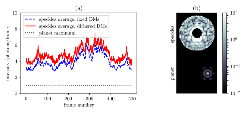
Figure 1: (a) Average intensity of the speckles in the dark hole (with and without dithering of the deformable mirrors) as it varies in time due to WFE drift. The maximum intensity of the planet is an order of magnitude below the speckle floor. (b) Side by side comparison of the speckles and the planet on a logarithmic scale. The data was obtained using a model of the WFIRST hybrid Lyot coronagraph implemented in FALCO (Riggs et al. (2018)).

The hybrid Lyot coronagraph starts at a relatively low contrast due to model/system imperfections. Therefore, as a precursor to the observation stage, the EFC (Give’on et al. (2007b)) algorithm was used to create a dark hole in a ring between $3$ and $9$ $\lambda/D$ with a nominal contrast of $4.2\cdot 10^{-10}$ at $\lambda=546\>\mathrm{nm}$ (to simplify the analysis, we discarded all electric fields of longer wavelengths that were simulated by FALCO). At this point, we introduced wavefront drift through independent random increments of the first $21$ Zernike polynomials,

$$\Delta z_{p}^{p-2j}(t)\sim{\cal N}\left(0,\frac{0.1\>\mathrm{nm}}{p^{2}\cdot\lambda}\right),\;0\leq j\leq p,$$ (24)

where $p$ is the order of the polynomial, $j$ is its azimuthal degree and $\Delta z_{p}^{p-2j}$ is its increment over one $100\>\mathrm{sec}$ frame. To make the comparison with PCA based methods (Soummer et al. (2012); Amara & Quanz (2012)) easier, we chose a Markov drift model in which the Zernike coefficients $z_{p}^{p-2i}(t)$ fluctuate but remain bounded at all times $t$,

$$z_{p}^{p-2j}(t)=0.99\cdot z_{p}^{p-2j}(t-1)+\Delta z_{p}^{p-2j}(t).$$ (25)

After creating the dark hole, but before “making” the observations, the Zenike coefficients where advanced $1000$ time steps via Eq. (25). Another potential source of high-order wavefront error is the time-dependent drift of the DM actuators themselves (J. T. Trauger, personal communication, 2019). Although not addressed here, its influence on the electric field would be linear and manifest itself through a low-rank approximation of the control Jacobian ($G^{U}$ instead of $G^{V}$ in Eq. (11)). Contrary to what one might expect, the “effective” rank of the Jacobian is far lower than the number of actuators, the latter being usually large to prevent actuator over-saturation.

The simulated data consisted of $500$ frames of the target star (with an exoplanet) and $1500$ frames of the reference star, which is more than sufficient for PCA purposes. The measurements were “taken” once with fixed DMs and once with DM dithering, while keeping the drift history, $z_{p}^{p-2i}(t)$, the same. The average intensity of the residual light was $1.2\>\mathrm{\frac{photons}{frame}}$ in a perfect dark hole, $4.8\>\mathrm{\frac{photons}{frame}}$ with simulated WFEs (time average), and $5.7\>\mathrm{\frac{photons}{frame}}$ with both WFEs and DM dithering. When pointing at the reference start, all speckle intensities where $16$ times higher. The maximum intensity of the planet was $1.0\>\mathrm{\frac{photons}{frame}}$ (see comparison in Fig. 1(b)) and the effective intensity of the dark current was $0.25\>\mathrm{\frac{photons}{frame}}$.

The total number of pixels in the dark hole (for the single wavelength considered) was $N=2608$. The history of the average dark hole intensity when observing the target star is shown in Fig. 1(a), with and without DM dithering (the dithering for each actuator was sampled from a normal distribution with $0.01$V standard deviation around their nominal values which had an average magnitude of $10$V). At each time frame, the number of photons detected at each pixel was sampled from a Poisson distribution based on the intensity of that pixel (Eq. (6)). We note that instead of just dithering the DMs, one could also apply an EFC control law to mitigate the effects of time-varying speckles (Pogorelyuk & Kasdin (2019)). This closed-loop approach would have resulted in higher contrast, lower shot noise, and a better post-processing factor; we plan to analyze the combined performance of EFOR and dark-hole maintenance in a future paper.

3.2 Results and Discussion

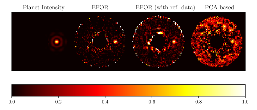
Figure 2: Planet intensity and its estimates by newly proposed Electric Field Order Reduction (EFOR) method (with and without a library of reference images) and by Principal Component Analysis (PCA; see Amara & Quanz (2012)). The images used by EFOR were simulated with an additional dithering of the DMs, but the underlying wavefront errors were the same.

Fig. 2 shows the best estimates of the incoherent intensity obtained by PCA and the EFOR method introduced in sec. 2. The PCA estimates were computed based on measurements taken with fixed DMs. The reference images were used to construct a basis for speckle intensities (via Singular Value Decomposition) across all pixels (although splitting the domain into smaller regions could reduce the optimal number of modes, see Soummer et al. (2012); Fergus et al. (2014)). The two EFOR estimates were obtained from measurements taken while dithering the DMs: one corresponds to fitting just the observations of the target star, and the other to fitting the observations to both the target and the reference stars (Eq. (17) vs. (22)). The latter estimate is slightly more accurate, illustrating the advantage of incorporating multiple observations. However, once one has a good estimate of the speckle basis, $\mathrm{\mathrm{colsp\left\{G^{V}\right\}}}$, additional reference images provide diminishing improvements in accuracy (similarly, PCA becomes insensitive to the number of reference images beyond a certain threshold).

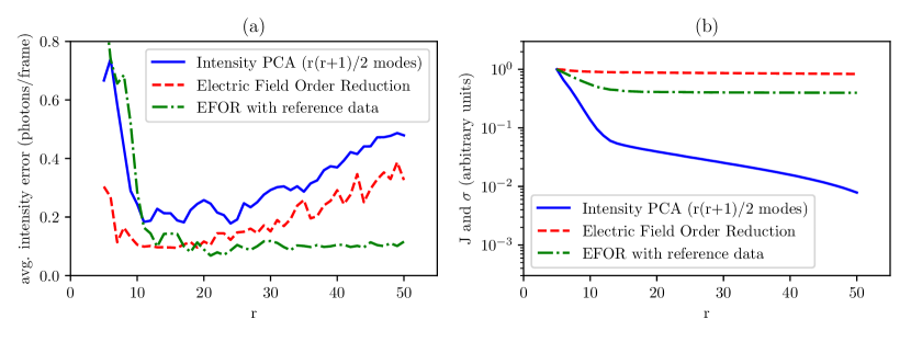
Figure 3: (a) Average errors in intensity estimates in planet’s half-max region ($I_{i}^{P}>0.5\left\|\mathbf{I}^{P}\right\|_{\infty}$), as a function of the number of electric field modes $r$ and the number of intensity modes $\frac{r(r+1)}{2}$. EFOR outperforms PCA by a factor of about $2.5$ when reference data is present. In the absence of reference data, EFOR tends to overfit the data when $r>r_{true}=22$. (b) Arbitrarily scaled residual errors of EFOR (the cost function in Eqs. (17) and (22)) and PCA (truncated singular value $\sigma$). The PCA and EFOR curves that are based on reference images suggest that the number of meaningful electric field modes is around $r=15$.

To make the comparison between the methods quantitative, consider the average error in the incoherent intensity estimate, $\mathbf{\hat{I}}^{P}$, in a region where the planet’s intensity is above its half-maximum,

$$\mathrm{err}\left(\mathbf{\hat{I}}^{P}\right)\equiv\mathrm{avg}\left\{\left.\left|\hat{I}_{i}^{P}-I_{i}^{P}\right|\right|1\leq i\leq N,\>I_{i}^{P}>0.5\left\|\mathbf{I}^{P}\right\|_{\infty}\right\}.$$ (26)

In Fig. 3(a), the errors in EFOR estimates are plotted as a function of the number of modes, $r$, while the errors in the PCA estimates are plotted as a function of $\frac{r(r+1)}{2}$ (in light of Eq. (9)). We indeed see that the errors of EFOR with reference data flatten around $r_{true}=22$ modes, while PCA reaches its peak accuracy in the region between $66$ and $300$ modes (corresponding to roughly $4r_{true}$ and $\frac{r_{true}(r_{true}+1)}{2}$, see discussion after Eq. (9)). EFOR without reference data, on the other hand, reaches its peak accuracy at around $r=15$ modes after which it overfits the data.

The lowest error, as defined by Eq. (26), is achieved by EFOR with reference data. The minimum error of EFOR with data from just the target start is $1.4$ times larger, while the lowest PCA error is $2.5$ times larger. These errors can be further reduced by incorporating more observations or employing a closed loop dark hole maintenance scheme (Pogorelyuk & Kasdin (2019)) to reduce the shot noise.

Finally, Fig. 3(b) shows the cost function $J$ of the EFOR methods and the truncated singular value of the PCA method as a function or $r$ and $\frac{r(r+1)}{2}$ respectively. The steep decrease in the EFOR’s cost function (with reference data) stops at $r=15$, suggesting that this is the number of “important” WFE modes. One would therefore expect the steep decrease in the singular values to stop somewhere between $4r=60$ and $\frac{r(r+1)}{2}=120$ PCA modes, and it indeed stops at around $\frac{12\cdot 13}{2}=78$ modes. In the case of a single observation sequence, the cost function of EFOR decreases very slowly (red dashed line on Fig. 3(b)) and doesn’t provide an indication of the “correct” number of modes, $r$. However, instead of using reference images, one could incorporate data from multiple targets to get a better estimate of the speckle field basis, $G^{V}$ (see discussion around Eq. (23)). Alternatively, one could choose the $r$ that maximizes some detection criterion based on the PSF of the planet/halo (e.g. a matched filter, Kasdin & Braems (2006), or a Hotelling observer, Caucci et al. (2007)).

4 Conclusions

In this work we assumed that the slow evolution of wavefront errors in space based coronagraphs can be well approximated by a small number of modes of the electric field in the pupil plane and that these errors are linearly propagated to the image plane. We then showed that a low-dimensional approximation of the speckles requires an order of magnitude fewer electric field modes than intensity modes. Consequently, we introduced a reduced-order algorithm for estimating the history of the electric field and the incoherent intensity (which includes the planet signal). Unlike existing methods (e.g. KLIP), our algorithm relies on small actuations (dithering) of the deformable mirrors during the observation phase as well as an accurate estimate of the controls influence matrix (the Jacobian). This introduces the phase diversity required for estimating the electric field, rather than the intensities of the speckles.

We illustrated that since the newly proposed method employs significantly fewer parameters, it has the potential to make substantially more accurate estimates than intensity-based PCA, even without a library of reference images. However, our method does allow for seamlessly incorporating reference data as well as other observations. The resulting scheme searches for an “optimal” basis for speckle field modes across all measurements taken by a given instrument.

More importantly, the proposed algorithm uniquely incorporates the history of control inputs employed during the observation phase. We speculate that combining it with a closed-loop dark hole maintenance scheme will decrease the shot noise and increase the post-processing factor even further. This direction, together with an analysis of the dithering strategy, are subjects of future research.

References

- Amara & Quanz (2012) Amara, A., & Quanz, S. P. 2012, Monthly Notices of the Royal Astronomical Society, 427, 948. https://dx.doi.org/10.1111/j.1365-2966.2012.21918.x
- Baba & Murakami (2003) Baba, N., & Murakami, N. 2003, Publications of the Astronomical Society of the Pacific, 115, 1363. https://doi.org/10.1086%2F380422
- Brock et al. (2016) Brock, A., Lim, T., Ritchie, J. M., & Weston, N. 2016, arXiv preprint arXiv:1609.07093
- Caucci et al. (2007) Caucci, L., Barrett, H. H., Devaney, N., & Rodríguez, J. J. 2007, J. Opt. Soc. Am. A, 24, B13. http://josaa.osa.org/abstract.cfm?URI=josaa-24-12-B13
- Cavarroc et al. (2006) Cavarroc, C., Boccaletti, A., Baudoz, P., Fusco, T., & Rouan, D. 2006, Astronomy & Astrophysics, 447, 397. https://doi.org/10.1051/0004-6361:20053916
- Codona & Kenworthy (2013) Codona, J. L., & Kenworthy, M. 2013, The Astrophysical Journal, 767, 100. https://doi.org/10.1088%2F0004-637x%2F767%2F2%2F100
- Codona et al. (2006) Codona, J. L., Kenworthy, M. A., Hinz, P. M., Angel, J. R. P., & Woolf, N. J. 2006, A high-contrast coronagraph for the MMT using phase apodization: design and observations at 5 microns and 2 lambda/D radius, , , doi:10.1117/12.672727. https://doi.org/10.1117/12.672727
- Demers (2018) Demers, R. 2018, in Space Telescopes and Instrumentation 2018: Optical, Infrared, and Millimeter Wave, Vol. 10698. https://doi.org/10.1117/12.2315632
- Demers et al. (2015) Demers, R. T., Dekens, F., Calvet, R., et al. 2015, in Techniques and Instrumentation for Detection of Exoplanets VII, Vol. 9605, International Society for Optics and Photonics, 960502. https://doi.org/10.1117/12.2191792
- Douglas et al. (2018) Douglas, E. S., Carlton, A. K., Cahoy, K. L., et al. 2018, in Modeling, Systems Engineering, and Project Management for Astronomy VIII, Vol. 10705, International Society for Optics and Photonics, 1070526
- Edelman et al. (1998) Edelman, A., Arias, T. A., & Smith, S. T. 1998, SIAM Journal on Matrix Analysis and Applications, 20, 303. https://doi.org/10.1137/s0895479895290954
- Fergus et al. (2014) Fergus, R., Hogg, D. W., Oppenheimer, R., Brenner, D., & Pueyo, L. 2014, The Astrophysical Journal, 794, 161. https://doi.org/10.1088%2F0004-637x%2F794%2F2%2F161
- Give’on et al. (2007a) Give’on, A., Kern, B., Shaklan, S., Moody, D. C., & Pueyo, L. 2007a, in Astronomical Adaptive Optics Systems and Applications III, Vol. 6691, International Society for Optics and Photonics, 66910A
- Give’on et al. (2007b) Give’on, A., Kern, B. D., Shaklan, S., Moody, D. C., & Pueyo, L. 2007b, in Bulletin of the American Astronomical Society, Vol. 39, 975
- Gonzalez et al. (2016) Gonzalez, C. A. G., Absil, O., Absil, P.-A., et al. 2016, Astronomy & Astrophysics, 589, A54. https://doi.org/10.1051/0004-6361/201527387
- Guyon (2005) Guyon, O. 2005, The Astrophysical Journal, 629, 592. https://doi.org/10.1086%2F431209
- Harding et al. (2015) Harding, L. K., Demers, R., Hoenk, M. E., et al. 2015, Journal of Astronomical Telescopes, Instruments, and Systems, 2, 1 . https://doi.org/10.1117/1.JATIS.2.1.011007
- Jovanovic et al. (2015) Jovanovic, N., Guyon, O., Martinache, F., et al. 2015, The Astrophysical Journal, 813, L24. https://doi.org/10.1088%2F2041-8205%2F813%2F2%2Fl24
- Jovanovic et al. (2018) Jovanovic, N., Absil, O., Baudoz, P., et al. 2018, Review of high-contrast imaging systems for current and future ground-based and space-based telescopes: Part II. Common path wavefront sensing/control and coherent differential imaging, , , doi:10.1117/12.2314260. https://doi.org/10.1117/12.2314260
- Kasdin & Braems (2006) Kasdin, N. J., & Braems, I. 2006, The Astrophysical Journal, 646, 1260. https://doi.org/10.1086%2F505017
- Kenworthy et al. (2007) Kenworthy, M. A., Codona, J. L., Hinz, P. M., et al. 2007, The Astrophysical Journal, 660, 762. https://doi.org/10.1086%2F513596
- Kingma & Ba (2014) Kingma, D. P., & Ba, J. 2014, arXiv preprint arXiv:1412.6980
- Lafreniere et al. (2007) Lafreniere, D., Marois, C., Doyon, R., Nadeau, D., & Artigau, E. 2007, The Astrophysical Journal, 660, 770. https://doi.org/10.1086%2F513180
- Marois et al. (2000) Marois, C., Doyon, R., Racine, R., & Nadeau, D. 2000, Publications of the Astronomical Society of the Pacific, 112, 91. https://doi.org/10.1086%2F316492
- Marois et al. (2006) Marois, C., Lafreniere, D., Doyon, R., Macintosh, B., & Nadeau, D. 2006, The Astrophysical Journal, 641, 556. https://doi.org/10.1086%2F500401
- Martinache (2010) Martinache, F. 2010, The Astrophysical Journal, 724, 464. https://doi.org/10.1088%2F0004-637x%2F724%2F1%2F464
- Mawet et al. (2012) Mawet, D., Pueyo, L., Lawson, P., et al. 2012, in Space Telescopes and Instrumentation 2012: Optical, Infrared, and Millimeter Wave, ed. M. C. Clampin, G. G. Fazio, H. A. MacEwen, & J. M. Oschmann (SPIE). https://doi.org/10.1117/12.927245
- Miller et al. (2017) Miller, K., Guyon, O., & Males, J. 2017, Journal of Astronomical Telescopes, Instruments, and Systems, 3, 1. https://doi.org/10.1117%2F1.jatis.3.4.049002
- Pogorelyuk & Kasdin (2019) Pogorelyuk, L., & Kasdin, N. J. 2019, The Astrophysical Journal, 873, 95. https://doi.org/10.3847/1538-4357/ab0461
- Pueyo (2018) Pueyo, L. 2018, Handbook of Exoplanets, 705
- Ren et al. (2018) Ren, B., Pueyo, L., Zhu, G. B., Debes, J., & Duchêne, G. 2018, The Astrophysical Journal, 852, 104. https://doi.org/10.3847%2F1538-4357%2Faaa1f2
- Riggs et al. (2018) Riggs, A. E., Ruane, G., Coker, C. T., et al. 2018, in Space Telescopes and Instrumentation 2018: Optical, Infrared, and Millimeter Wave, ed. H. A. MacEwen, M. Lystrup, G. G. Fazio, N. Batalha, E. C. Tong, & N. Siegler (SPIE). https://doi.org/10.1117/12.2313812
- Shaklan et al. (2011) Shaklan, S. B., Marchen, L., Krist, J. E., & Rud, M. 2011, in Techniques and Instrumentation for Detection of Exoplanets V, Vol. 8151, International Society for Optics and Photonics, 815109. https://doi.org/10.1117/12.892838
- Soummer et al. (2012) Soummer, R., Pueyo, L., & Larkin, J. 2012, The Astrophysical Journal Letters, 755, L28. https://doi.org/10.1088%2F2041-8205%2F755%2F2%2Fl28
- Sparks & Ford (2002) Sparks, W. B., & Ford, H. C. 2002, The Astrophysical Journal, 578, 543. https://doi.org/10.1086/342401
- Sun et al. (2018) Sun, H., Kasdin, N. J., & Vanderbei, R. 2018, Journal of Astronomical Telescopes, Instruments, and Systems, 4, 1. https://doi.org/10.1117/1.jatis.4.4.049006
- Townsend et al. (2016) Townsend, J., Koep, N., & Weichwald, S. 2016, Journal of Machine Learning Research, 17, 1. http://jmlr.org/papers/v17/16-177.html
- Ygouf et al. (2016) Ygouf, M., Zimmerman, N. T., Pueyo, L., et al. 2016, in Space Telescopes and Instrumentation 2016: Optical, Infrared, and Millimeter Wave, ed. H. A. MacEwen, G. G. Fazio, M. Lystrup, N. Batalha, N. Siegler, & E. C. Tong (SPIE). https://doi.org/10.1117/12.2231581