The Receptive Field as a Regularizer
in Deep Convolutional Neural Networks
for Acoustic Scene Classification

Abstract

Convolutional Neural Networks (CNNs) have had great success in many machine vision as well as machine audition tasks. Many image recognition network architectures have consequently been adapted for audio processing tasks. However, despite some successes, the performance of many of these did not translate from the image to the audio domain. For example, very deep architectures such as ResNet [1] and DenseNet [2], which significantly outperform VGG [3] in image recognition, do not perform better in audio processing tasks such as Acoustic Scene Classification (ASC). In this paper, we investigate the reasons why such powerful architectures perform worse in ASC compared to simpler models (e.g., VGG). To this end, we analyse the receptive field (RF) of these CNNs and demonstrate the importance of the RF to the generalization capability of the models. Using our receptive field analysis, we adapt both ResNet and DenseNet, achieving state-of-the-art performance and eventually outperforming the VGG-based models. We introduce systematic ways of adapting the RF in CNNs, and present results on three data sets that show how changing the RF over the time and frequency dimensions affects a model’s performance. Our experimental results show that very small or very large RFs can cause performance degradation, but deep models can be made to generalize well by carefully choosing an appropriate RF size within a certain range.

I Introduction and Related Work

2019 IEEE. Personal use of this material is permitted. Permission from IEEE must be obtained for all other uses, in any current or future media, including reprinting/republishing this material for advertising or promotional purposes, creating new collective works, for resale or redistribution to servers or lists, or reuse of any copyrighted component of this work in other works.

In image processing, deep Convolutional Neural Networks (CNNs) have revolutionized the way image recognition tasks are addressed. A central source of their power is the ability to learn multi-level internal features and representations. While lower-level network layers learn to detect simple features such as edges, deeper layers combine these features to detect higher-level concepts such as textures, shapes, and objects.

The current state of the art in this domain are ResNet [1] and DenseNet [2] variants, which outperform earlier (and less deep) VGG-based [3] architectures by a significant margin. This is mainly because they address shortcomings of VGG such as the vanishing gradient. However, in acoustic tasks (e.g., Acoustic Scene Classification; ASC) the state of the art is still heavily dominated by VGG-like architectures [4, 5, 6, 7].

For instance, Eghbal-zadeh et al. [4] adapted the VGG architecture taken from the computer vision domain and achieved good performance in acoustic scene classification, using spectrograms as network input. Hershey et al. [8] compared various well-known image recognition CNN architectures on a large-scale dataset of 70M audio clips from YouTube. They showed that on such a large dataset, very deep CNNs such as ResNet-50 can perform very well. However, as we will show later, training such deep architectures on smaller datasets results in heavy overfitting on the training samples. Because of this issue, many state-of-the-art ASC systems use shallower CNN architectures [4, 8, 5, 6, 7, 9, 10, 11, 12]. Pons et al. [13] investigated the effect of filter shapes in shallow CNN architectures in music classification tasks. They proposed to change the shape of convolutional filters in order to restrict CNNs to learn either temporal or frequency dependencies in the data.

In this paper, we systematically investigate the effect of restricting the Receptive Field (RF) on the time or the frequency dimensions in deep and complex CNN architectures. We show that for relatively smaller datasets, CNNs tend to overfit if their RF covers large areas of the spectrograms. Moreover, limiting the RF over the frequency dimension helps output neurons generalize better to unseen samples. We introduce an approach to adapt deep CNN architectures for ASC by restricting their RF, since the RF grows when the depth of a CNN increases. We apply this method on a deep DenseNet [2] and ResNet [1] architecture and compare classification performance before and after this adaptation. Furthermore, we modify a number of convolutional layers in a ResNet architecture by changing their filter shapes to obtain a specific RF. The filter shape controls the RF of its layer over the time or frequency dimensions, while the number of modified layers controls the RF of the whole network. This technique allows us to study how gradually increasing the RF of a CNN affects its performance.

II The Effect of the Receptive Field

II-A The Receptive Field in CNNs

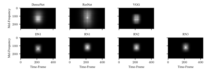
Figure 1: The Effective Receptive Field (ERF) of different CNN architectures trained on DCASE18 (explained in Section IV-A).

In fully-connected layers, each neuron is affected by the whole input. In contrast, in convolutional layers each neuron has a strictly limited ‘field of view’ (RF); input values outside of this RF cannot influence the neuron’s activation. The RF in general includes input values in the spatial as well as the channels dimensions. However, in this paper, we will keep our focus on the spatial dimensions (the frequency and the time dimension of spectrograms, in the case of audio).

Within a convolutional layer, the spatial RF of a neuron is determined by its filter size: the bigger the filter, the more activations it can see from the previous layer. As the CNN’s depth increases by stacking more convolutional layers, the RF of a neuron w.r.t. the input layer – that is, what the neuron ‘sees’ of the input layer – is affected by various factors such as the filter size, the stride and the dilatation of all the previous layers. The maximum RF size can be calculated using the following equation:

$$\begin{array}[]{l}S_{n}=S_{n-1}*s_{n}\\ RF_{n}=RF_{n-1}+(k_{n}-1)*S_{n}\end{array}$$ (1)

where $s_{n}$, $k_{n}$ are stride and kernel size of layer $n$, respectively, and $S_{n}$, $RF_{n}$ are cumulative stride and RF of a unit from layer $n$ to the network input. While the formula above gives the maximum RF each neuron has access to, a given neuron may not actually use all of it. The set of input pixels or units that effectively influence a neuron is called its Effective Receptive Field (ERF). Luo et al. [14] showed that neurons are more affected by the input pixels around the center of the RF, since these have more paths to the neuron on both the forward and the backward pass. This is important considering that in some cases the maximum RF of a network even exceeds the input dimensions. Further, they propose a method for computing the Effective Receptive Field (ERF) of a trained model. They back-propagate a gradient signal from the output layer through the network to the input. In order to compute the ERF on models trained on audio spectrograms, we follow the approach proposed by Luo et al. [14]. We back-propagate a gradient signal of 1 in one output spatial pixel (i.e. before the global averaging) to the inputs. For visualisation, we average this gradient for all the test set samples and plot the normalized average. Figure 1 shows the ERF for different CNNs trained on the ASC task, the details of their architectures is explained in Section IV-A. As can be seen, the ERFs can be vastly different depending on the network architecture.

II-B Modifying the Receptive Field of a CNN

Equation (1) shows that there are various ways to modify the RF of a CNN. In this paper, we investigate how changing the RF influences the performance of a model in the task of acoustic scene classification. In order to achieve this goal, we follow two approaches to change the RF either by altering the filter sizes or by adding sub-sampling layers. We detail these two approaches as follows.

II-B1 Changing the filter sizes

Starting from a CNN architecture we change the filter sizes of some layers $k_{n}$ from 3x3 to 1x1. One side effect of changing the filter sizes, is that it changes the number of network parameters.

II-B2 Changing the sub-sampling layers

We add more max-pooling layers to increase the accumulative stride $S_{n}$. This results in changing the RF on the network, without changing the network’s number of parameters.

III Experimental Setup

In this section we detail the datasets, architectures and training procedure we follow in our experiments.

III-A Datasets

We tested our hypotheses on multiple datasets with different properties, scales, and of increasing difficulty.

III-A1 DCASE2016

The acoustic scenes classification task of DCASE 2016 [15] is to recognise 15 possible acoustic scenes from $30$ second snippets of audio. There are $1170$ training and $390$ test examples, for a total of 9 hours 45 minutes of training data and 3 hours 15 minutes for evaluation.

III-A2 DCASE2017

The DCASE 2017 [16] training set comprises both the training and evaluation sets of DCASE 2016. The evaluation data is a set of new recordings taken at a later time. This introduces a distribution mismatch between the training and unseen test data, making for a more difficult learning task. Additionally, the audio clips are cut into 10 seconds samples totaling 4680 training samples (13 hours) and 1620 testing samples (4.5 hours).

III-A3 DCASE2018

DCASE 2018 Task 1 [17] consists of around 17 hours of audio for training (6122 10-second clips) and 7 hours for evaluation (2518 10-second clips). The data was recorded in more diverse locations compared to the previous challenges. Each recording belongs to one out of 10 possible classes.

III-B Network Architectures

For our experimental investigations, we used three different CNN architectures which were successful in the computer vision domain.

III-B1 VGG

Architectures similar to VGG [3] are very popular in the DCASE community and the audio processing community in general. This is mainly due to their good performance in tasks such as ASC [4, 5, 6, 7], audio tagging [9, 10], and event detection [11, 12]. We make an effort to explain this good performance by the fact that deeper CNNs have a bigger RF as explained in Section V.

III-B2 ResNet

ResNet [1] adds residual connections between convolutional layers, this counters the vanishing gradient problem of deep CNNs. It outperforms VGG in computer vision tasks. In contrast, top performing systems in acoustic scene classification DCASE challenges [4, 6, 7] are still based on VGG variants. We will show in Section III how we adapted ResNet-28 (with 28 layers) to finally outperform VGG models.

III-B3 DenseNet

DenseNet [2] solves the vanishing gradient problem by concatenating the outputs of all previous convolution layers on the channels dimension. DenseNet variants achieves state-of-the-art results on computer vision tasks.

III-C Setup

For all experiments, we set up our training framework following the current state of the art [6, 7]. All the experiments used the same setup, to ensure a fair comparison.

III-C1 Data Preparation

The input is down-sampled to 22.05 kHz and subjected to a Short Time Fourier Transform (STFT) with a window size of 2048 and 25% overlap, followed by a Mel-scaled filter bank on perceptually weighted spectrograms. That results in 256 Mel frequency bins and around 43 frames per second. The input frames are normalized to zero-mean and unit variance according to the training set.

III-C2 Optimizing

The Adam optimizer [18] is used for a total of 350 epochs, with a starting learning rate of $1\times 10^{-4}$. The learning rate decays linearly from epoch 50 until 250 where it reaches $5\times 10^{-6}$. Then we train for another 100 epochs with the minimum learning rate $5\times 10^{-6}$.

III-C3 Data Augmentation

We use mix-up [19] since it was shown to improve the generalization of the models and to help in preventing overfitting.

III-C4 Obtaining Results

The models are evaluated on the test set after 350 epochs of training. By using mix-up and batch normalization in the architectures, we ensure that models are not overfitting on the training set. Each experiment is repeated 3 times for Table I and 6 times for Figure 2. We report the mean and the standard deviation of these runs.

IV Experiments

IV-A Modifying the “Vision Architectures”

In this section we report on a series of experiment whose purpose is to investigate the effect of the RF on the performance of a CNN architecture. In particular, we investigate how and to what extent we can push a CNN’s generalization by calibrating its RF. We do this by evaluating modified ResNets and DenseNets on several benchmark datasets from the world of acoustic scene classification.

Table I shows the performance of the “vision architectures” ResNet and DenseNet before and after adjusting the RF to match the VGG-like architecture proposed by Dorfer et al. [6]. We modified the deep architectures from Section III-B to obtain similar RFs as [6], as described below. These straight-forward modifications boost the performance across all architecture and datasets. The adopted models outperform both the VGG baseline as well as their vision-inspired predecessors.

IV-A1 ResNet

ResNet is usually deeper than VGG, and thus has a larger receptive field. There are many ways to modify ResNet to have a smaller RF; we chose the following:

TABLE I: Architectures performance on DCASE datasets

	DCASE16	DCASE17	DCASE18
	Loss
DenseNet [2]	$0.58\pm 0.02$	$1.31\pm 0.17$	$0.92\pm 0.04$
ResNet [1]	$0.67\pm 0.06$	$1.19\pm 0.06$	$1.02\pm 0.05$
VGG [3, 6]	$0.69\pm 0.05$	$1.05\pm 0.04$	$0.83\pm 0.03$
RN1	$0.57\pm 0.02$	$0.94\pm 0.09$	$0.67\pm 0.03$
RN2	$0.50\pm 0.02$	$0.91\pm 0.04$	$0.71\pm 0.03$
RN3	$0.53\pm 0.04$	$0.89\pm 0.02$	$0.67\pm 0.00$
DN1	$0.51\pm 0.01$	$0.90\pm 0.04$	$0.72\pm 0.06$
	Accuracy
DenseNet [2]	$83.68\pm 0.90$	$63.48\pm 4.96$	$71.55\pm 0.85$
ResNet [1]	$83.17\pm 0.91$	$67.19\pm 1.72$	$71.05\pm 0.87$
VGG [3, 6]	$82.99\pm 0.90$	$67.90\pm 1.31$	$74.56\pm 1.01$
RN1	$85.98\pm 1.32$	$71.11\pm 1.19$	$77.34\pm 1.53$
RN2	$87.09\pm 0.53$	$72.41\pm 0.96$	$75.71\pm 0.70$
RN3	$86.51\pm 1.05$	$71.74\pm 0.85$	$77.61\pm 0.22$
DN1	$86.07\pm 0.65$	$72.24\pm 1.00$	$76.39\pm 0.14$

• Making ResNet shallower (RN1 in Table II) We removed tailing layers from ResNet after the RF of [6] is reached. The resulting network looks similar to VGG, but with residual connections; the network consists of 5 residual blocks of two convolutional layers each. The resulting network has a total of $3,258,772$ trainable parameters, since we did not change the number of channels in the new network.

• Changing filter sizes (RN2 in Table II) Instead of removing layers from ResNet, We changed some filter sizes from $3\times 3$ to $1\times 1$. Network RN2 has $12$ residual blocks of two convolutional layers each. $7$ residual blocks have $3\times 3$ filters in the first convolutional layer and $1\times 1$ and the second layer; the rest of the residual blocks consist only of $1\times 1$ convolutions. In other words, we kept the depth of ResNet but changed many filter sizes to $1\times 1$. RN2 has a total number of parameters of $6,053,780$.

• Changing the sizes of the tailing filters RN3 is similar to RN1, except that we do not delete the tailing layers but instead only change their filter sizes to $1\times 1$.

TABLE II: Modified ResNet architectures

RB Number	RB Config
	RN1	RN2	RN3
	Input $5\times 5$ stride=$2$
1	$3\times 3$, $1\times 1$, P	$3\times 3$, $1\times 1$, P	$3\times 3$, $1\times 1$, P
2	$3\times 3$, $3\times 3$, P	$3\times 3$, $1\times 1$	$3\times 3$, $3\times 3$, P
3	$3\times 3$, $3\times 3$,	$3\times 3$, $1\times 1$	$3\times 3$, $3\times 3$
4		$1\times 1$, $1\times 1$, P	$3\times 3$, $3\times 3$, P
5	$3\times 3$, $3\times 3$, P	$3\times 3$, $1\times 1$	$3\times 3$, $1\times 1$
6		$3\times 3$, $1\times 1$	$1\times 1$, $1\times 1$
7		$3\times 3$, $1\times 1$	$1\times 1$, $1\times 1$
8		$3\times 3$, $1\times 1$, P	$1\times 1$, $1\times 1$
9	$3\times 3$, $1\times 1$	$3\times 3$, $1\times 1$	$1\times 1$, $1\times 1$
10		$1\times 1$, $1\times 1$	$1\times 1$, $1\times 1$
11		$1\times 1$, $1\times 1$	$1\times 1$, $1\times 1$
12		$1\times 1$, $1\times 1$	$1\times 1$, $1\times 1$
RB: Residual Block, P: $2\times 2$ max pooling after the block.
RB number 1-4 have 128 channels, RB number 5-8 have 256 channels,
RB number 9-12 have 512 channels.

IV-A2 DenseNet

Unlike ResNet and VGG, estimating the effective RF of DenseNet is non-trivial. It cannot be inferred directly from the maximum possible RF (1) because of the dense connections [2]. Each convolutional layer projects its input into feature maps with a small number of channels (the ‘growth rate’ in  [2]). This will increase the maximum RF but will have a small effect since only few feature maps have this RF. We increased the growth rate to 128 and reduced the network depth in order for its maximum RF to match Dorfer et al. [6]. The resulting network DN1 has $5,269,902$ parameters.

IV-B The Effect of Systematic Changes of the RF

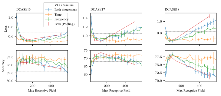
Figure 2: The effects of systematic changes to the receptive field of ResNet (averages and std. deviations over 6 runs). The dashed horizontal line is the loss/accuracy achieved by the current state-of-the-art VGG architecture in this field [6, 9].

For more detailed insight, Fig. 2 shows the testing loss and accuracy for various configurations of our ResNet, modified by systematically varying the network filters or the pooling:

IV-B1 Changing filters in both dimensions

Starting from the last layer of a network with all $3\times 3$ filters, we modify the filters from $3\times 3$ to $1\times 1$. This will affect the RF on both dimensions, and results in networks with maximum RFs (Section II) ranging from $23\times 23$ to $583\times 583$ pixels.

IV-B2 Changing filters in the time dimension only

Here, we fix the RF on the frequency dimension to the one in the Dorfer et al. model [6] (i.e., 135 pixels). We only change the filter sizes in the time dimension. This results in networks with maximum RFs ranging from $23\times 135$ to $583\times 135$ pixels.

IV-B3 Changing filters in the frequency dimension

The procedure is analogous to the previous one, but using the frequency dimension instead of time. This results in networks with maximum RFs ranging from $135\times 23$ to $135\times 583$ pixels.

IV-B4 Changing pooling layers

Here, we add or remove pooling layers. Pooling layers have a stride of 2; adding one thus doubles accumulative stride (see Eq. (1)) in all layers that follow the pooling. Pooling layers do not affect the number of parameters of the network, hence we use them to demonstrate the effect of the RF without changing the number of parameters. However, adding a pooling layer downsamples the spatial dimensions by the provided factor and the RF of all subsequent layers will be affected by this change. Because of these architectural limitations, we only provide the feasible steps in this experiment. Figure 2 shows the results of networks with RFs of $67\times 67$, $135\times 135$, and $507\times 507$.

V Discussion

V-A The Effect of the Receptive Field

Figure 2 shows the effect of systematic changes to the RF, on three ASC datasets. It can be seen that there is a certain range of RF sizes that permit the CNN to generalize and predict well. On the one hand, RFs that are too small impair the CNN’s performance. Our intuition is that output neurons do not collect enough information to make the optimal decision and thus underfit even the training data. On the other hand, when the RF grows larger than this range – usually in the case of the CNN growing deeper – the CNN overfits the training data and fails to generalize to new samples. We observed this in the training loss (not reported) which decreases the bigger the RF is, while the performance deteriorates. This effect is more clear in DCASE17 and DCASE18 compared to DCASE16. We explain this with the characteristics of the datasets: in DCASE16, the test set has a similar distribution to the training set, while in DCASE17 and DCASE18 the impact of a (non-)optimal RF is magnified because of the distribution mismatch between the test and training sets.

V-B The Effect of Changing the RF over one Dimension

The plots also show that an optimal RF over the frequency dimension makes the effect of increasing the RF over the time dimension surprisingly minimal, provided that it is large enough to capture the necessary information. A possible reason may be that the training datasets have enough variance in the temporal dimension of the learned features so that the model does not overfit on long-term temporal dependencies in the data. However, the opposite happens when shrinking/extending the RF on the frequency dimension, despite an optimal RF over time. Seeing the whole frequency range seems to lead the CNN to overfit on the training data’s acoustic events, which may differ in some frequency bins in the test recordings.

V-C The Influence of the Number of Parameters

Finally, we see that using different CNNs with the same number of parameters but with different RFs (Section IV-B4) results in a performance that correlates with the results of the previous section. This indicates that the effect on overfitting of a larger RF is more significant than the number of parameters for a given architecture. For example, RN1, RN2 and RN3 have different numbers of parameters but the same RF; they perform similarly compared to other architectures.

VI Conclusion

We investigated the relation between CNNs’ RFs over the input spectrograms and their generalization on unseen samples, for the acoustic scene classification task. We showed that a large RF especially over the frequency dimension pushes CNNs to overfit, while a smaller than necessary RF forces a CNN to underfit the data and prevents it from learning decisive features. Although many factors contribute to a CNN’s tendency to generalize, we show that for a specific training setup and network architecture, tuning the RF of the model is a crucial factor for its performance. Following these guidelines, we managed to tune state-of-the-art vision architectures that so far failed to perform well on ASC, to match and outperform current popular and state-of-the-art CNNs on this task.

References

- [1] K. He, X. Zhang, S. Ren, and J. Sun, “Deep residual learning for image recognition,” in Proceedings of the IEEE Conference on Computer Vision and Pattern Recognition, pp. 770–778.
- [2] G. Huang, Z. Liu, L. Van Der Maaten, and K. Q. Weinberger, “Densely connected convolutional networks,” in Proceedings of the IEEE Conference on Computer Vision and Pattern Recognition, pp. 4700–4708.
- [3] K. Simonyan and A. Zisserman, “Very Deep Convolutional Networks for Large-Scale Image Recognition.” [Online]. Available: http://arxiv.org/abs/1409.1556
- [4] H. Eghbal-Zadeh, B. Lehner, M. Dorfer, and G. Widmer, “CP-JKU submissions for DCASE-2016: A hybrid approach using binaural i-vectors and deep convolutional neural networks.” DCASE2016 Challenge.
- [5] B. Lehner, H. Eghbal-Zadeh, M. Dorfer, F. Korzeniowski, K. Koutini, and G. Widmer, “Classifying short acoustic scenes with I-vectors and CNNs: Challenges and optimisations for the 2017 DCASE ASC task.” DCASE2017 Challenge.
- [6] M. Dorfer, B. Lehner, H. Eghbal-zadeh, C. Heindl, F. Paischer, and G. Widmer, “Acoustic Scene Classification with Fully Convolutional Neural Networks and I-Vectors.” DCASE2018 Challenge.
- [7] Y. Sakashita and M. Aono, “Acoustic Scene Classification by Ensemble of Spectrograms Based on Adaptive Temporal Divisions.” DCASE2018 Challenge.
- [8] S. Hershey, S. Chaudhuri, D. P. W. Ellis, J. F. Gemmeke, A. Jansen, R. C. Moore, M. Plakal, D. Platt, R. A. Saurous, B. Seybold, M. Slaney, R. J. Weiss, and K. Wilson, “CNN architectures for large-scale audio classification,” in 2017 IEEE International Conference on Acoustics, Speech and Signal Processing (ICASSP), pp. 131–135.
- [9] M. Dorfer and G. Widmer, “Training general-purpose audio tagging networks with noisy labels and iterative self-verification,” in Proceedings of the Detection and Classification of Acoustic Scenes and Events 2018 Workshop (DCASE2018), pp. 178–182.
- [10] T. Iqbal, Q. Kong, M. Plumbley, and W. Wang, “Stacked Convolutional Neural Networks for General-purpose Audio Tagging.” DCASE2018 Challenge.
- [11] D. Lee, S. Lee, Y. Han, and K. Lee, “Ensemble of Convolutional Neural Networks for Weakly-Supervised Sound Event Detection Using Multiple Scale Input.” DCASE2017 Challenge.
- [12] K. Koutini, H. Eghbal-zadeh, and G. Widmer, “Iterative knowledge distillation in R-CNNs for weakly-labeled semi-supervised sound event detection,” in Proceedings of the Detection and Classification of Acoustic Scenes and Events 2018 Workshop (DCASE2018), pp. 173–177.
- [13] J. Pons, T. Lidy, and X. Serra, “Experimenting with musically motivated convolutional neural networks,” in 2016 14th International Workshop on Content-Based Multimedia Indexing (CBMI), pp. 1–6.
- [14] W. Luo, Y. Li, R. Urtasun, and R. Zemel, “Understanding the Effective Receptive Field in Deep Convolutional Neural Networks,” in Advances in Neural Information Processing Systems 29, pp. 4898–4906.
- [15] A. Mesaros, T. Heittola, and T. Virtanen, “TUT database for acoustic scene classification and sound event detection,” in Signal Processing Conference (EUSIPCO), 2016 24th European. IEEE, pp. 1128–1132.
- [16] A. Mesaros, T. Heittola, A. Diment, B. Elizalde, A. Shah, E. Vincent, B. Raj, and T. Virtanen, “DCASE 2017 challenge setup: Tasks, datasets and baseline system,” in DCASE 2017-Workshop on Detection and Classification of Acoustic Scenes and Events.
- [17] A. Mesaros, T. Heittola, and T. Virtanen, “A multi-device dataset for urban acoustic scene classification,” in Proceedings of the Detection and Classification of Acoustic Scenes and Events 2018 Workshop (DCASE2018), pp. 9–13.
- [18] D. P. Kingma and J. Ba, “Adam: A Method for Stochastic Optimization.” [Online]. Available: http://arxiv.org/abs/1412.6980
- [19] H. Zhang, M. Cisse, Y. N. Dauphin, and D. Lopez-Paz, “Mixup: Beyond Empirical Risk Minimization.” [Online]. Available: http://arxiv.org/abs/1710.09412