Three-body interaction near a narrow two-body zero crossing

Abstract

We calculate the effective three-body force for bosons interacting with each other by a two-body potential tuned to a narrow zero crossing in any dimension. We use the standard two-channel model parametrized by the background atom-atom interaction strength, the amplitude of the open-channel to closed-channel coupling, and the atom-dimer interaction strength. The three-body force originates from the atom-dimer interaction, but it can be dramatically enhanced for narrow crossings, i.e., for small atom-dimer conversion amplitudes. This effect can be used to stabilize quasi-two-dimensional dipolar atoms and molecules.

I Introduction

In recent years, dilute weakly interacting bosons with intentionally weakened mean-field interactions have become one of the main attractions in the field of quantum gases. The weakness of the mean-field interaction in such systems makes higher-order terms relatively more important leading to dramatic effects. A prominent example is the observation of dilute quantum droplets in dipolar atoms Kadau2016 ; Schmitt2016 ; Ferrier2016 ; Chomaz2016 and in nondipolar mixtures Cabrera2017 ; Cheiney2018 ; Semeghini2018 . Two-body interactions of different kinds (contact and dipole-dipole in the dipolar case and interspecies and intraspecies in the mixture case) are tuned to compete with each other such that the resulting weak overall attraction gets compensated by a higher-order Lee-Huang-Yang (LHY) term PetrovLHY2015 ; Wachtler2016 ; Bisset2016 . An impressive experimental progress has been made in the dipolar case on pursuing supersolidity through the formation of coherent arrays of quantum droplets Tanzi2019 ; Chomaz2019 ; Bottcher2019 ; Tanzi2019Modes ; Guo2019 .

All these achievements correspond to essentially three-dimensional setups well described by the Gross-Pitaevskii energy density functional with an additional local LHY term $\propto n^{5/2}$, where $n$ is the density. However, there are various reasons to consider other configurations where the $n^{5/2}$ term is absent or too weak (low-dimensional geometries, single-component contact-interacting atoms, etc.) In these cases, an effective three-body interaction, associated with a $n^{3}$ term in the energy density, can become dominant if the leading-order two-body forces are suppressed. In particular, three-body forces have been considered in the context of droplet formation in three dimensions Bulgac2002 ; PetrovThreeBody2014 ; Xi2016 ; Bisset2015 and as a means for stabilizing supersolid phases of quasi-two-dimensional dipolar atoms or molecules Lu2015 . Quite a few recent theory papers have discussed one-dimensional three-body-interacting systems, exploring the kinematic equivalence of the three-body scattering in one dimension and the two-body scattering in two dimensions (see, for example, Refs. PricoupenkoJr2018 ; Sekino2018 ; Drut2018 ; Nishida2018 ; Pricoupenko2018 ; Guijarro2018 ; Pricoupenko2019 ; Daza2018 ; McKenney2019 ; Pastukhov2019 ; Valiente2019 ; ValientePastukhov2019 ).

In this paper we analyze a simple mechanism for the emergence of an effective three-body interaction. Namely, we consider bosons interacting with each other by a potential tuned to a zero crossing near a narrow Feshbach resonance, where the conversion amplitude from atoms to closed-channel dimers is small and where the two-body scattering amplitude is characterized by a large effective range $R_{\rm e}$. The effective three-body force appears in this model when one takes into account the interaction between atoms and closed-channel dimers, characterized by the coupling strength $g_{12}$. We find that the three-body coupling constant $g_{3}$ in $D$ dimensions is proportional to $R_{\rm e}^{D}g_{12}$ and can thus be enhanced near narrow two-body zero crossings.

The paper is organized as follows. In Sec. II we introduce the two-channel model and perform its mean-field analysis. In the dilute limit the density of closed-channel dimers in the system scales as $R_{\rm e}^{D}n^{2}\ll n$ and the effective three-body interaction emerges simply as the atom-dimer mean-field interaction energy $\propto R_{\rm e}^{D}g_{12}n^{3}$. We show that this simple mechanism, applied to two-dimensional dipoles, generates conditions for observing supersolid phases predicted in Ref. Lu2015 .

In Secs. III and IV we turn to the few-body perspective and perform a detailed nonperturbative analysis of the two-body (Sec. III) and three-body (Sec. IV) problems with zero-range potentials. In particular, the three-body scattering length near a narrow two-body zero crossing is found for an arbitrary atom-dimer interaction strength in any dimension.

II Mean-field analysis

We start with the two-channel model described by the Hamiltonian Radzihovsky2008

$$\hat{H}=\int_{\bf r}\Big{\{}-\hat{\psi}_{1}^{\dagger}({\bf r})\frac{\nabla^{2}}{2}\hat{\psi}_{1}({\bf r})+\hat{\psi}_{2}^{\dagger}({\bf r})\left(-\frac{\nabla^{2}}{4}+\nu_{0}\right)\hat{\psi}_{2}({\bf r})$$

$$-\frac{\alpha}{2}[\hat{\psi}_{1}^{\dagger}({\bf r})\hat{\psi}_{1}^{\dagger}({\bf r})\hat{\psi}_{2}({\bf r})+{\rm h.c.}]+\sum_{\sigma\sigma^{\prime}}\frac{g_{\sigma\sigma^{\prime}}}{2}\hat{n}_{\sigma}({\bf r})\hat{n}_{\sigma^{\prime}}({\bf r})\Big{\}},$$ (1)

where $\hat{\psi}_{1}$ and $\hat{\psi}_{2}$ are, respectively, the annihilation operators of atoms and dimers, $\hat{n}_{\sigma}$ are the corresponding density operators, $\nu_{0}$ is the detuning parameter, $g_{\sigma\sigma^{\prime}}$ are interaction constants, $\alpha$ is the atom-dimer conversion amplitude (without loss of generality assumed real and positive), and we have set $\hbar$ and atom mass equal to 1. Hereafter, $\int_{\bf r}$ denotes $\int d^{D}r$.

In the mean-field description of (1) we assume pure atomic and molecular condensates $\hat{\psi}_{\sigma}=\sqrt{n_{\sigma}}$ with the same phase (which corresponds to the energy minimum for $\alpha>0$) Radzihovsky2008 . We arrive at the energy density

$$E/L^{D}=\nu_{0}n_{2}-\alpha n_{1}\sqrt{n_{2}}+\sum_{\sigma\sigma^{\prime}}g_{\sigma\sigma^{\prime}}{n}_{\sigma}{n}_{\sigma^{\prime}}/2,$$ (2)

which we minimize with respect to $n_{2}$ (or $n_{1}$) keeping the total density $n=n_{1}+2n_{2}$ constant. For positive $\nu_{0}$ and small $n$ the dimer population behaves quadratically in $n$

$$n_{2}=\left(\frac{\alpha n}{2\nu_{0}}\right)^{2}\left(1+\frac{4g_{11}\nu_{0}-2g_{12}\nu_{0}-3\alpha^{2}}{\nu_{0}^{2}}n\right)+O(n^{4})$$ (3)

and the energy density reads

$$\frac{E}{L^{D}}=\left(\frac{g_{11}}{2}-\frac{\alpha^{2}}{4\nu_{0}}\right)\left(n^{2}-\frac{\alpha^{2}}{\nu_{0}^{2}}n^{3}\right)+\frac{g_{12}\alpha^{2}}{4\nu_{0}^{2}}n^{3}+O(n^{4}).$$ (4)

The two-body zero crossing occurs at the detuning $\nu_{0}=\alpha^{2}/2g_{11}$ where the first term in the right-hand side of Eq. (4) vanishes. One can then see that the residual three-body energy shift originates from the direct mean-field interaction of atoms with dimers. It equals $g_{12}n_{1}n_{2}\approx g_{3}n^{3}/3!$ with

$$g_{3}=6g_{12}g_{11}^{2}/\alpha^{2}=3g_{12}R_{\rm e}^{D}.$$ (5)

The effective volume $R_{\rm e}^{D}=2g_{11}^{2}/\alpha^{2}$ introduced in Eq. (5) characterizes the closed-channel population. Indeed, the density of dimers can be written as

$$n_{2}\approx R_{\rm e}^{D}n^{2}/2$$ (6)

meaning that each pair of atoms is found in the closed-channel dimer state with probability $(R_{\rm e}/L)^{D}$.

If $g_{\sigma\sigma^{\prime}}$ are of the same order of magnitude $\sim g$, the expansion (4) is in powers of $R_{\rm e}^{D}n$, which we assume small. Then, at the zero crossing the three-body term gives the leading contribution to the energy density $\sim gn^{2}(R_{\rm e}^{D}n)^{1}$ and we neglect subleading terms such as, for instance, the dimer-dimer interaction $\sim g_{22}\alpha^{4}n^{4}/\nu_{0}^{4}\sim gn^{2}(R_{\rm e}^{D}n)^{2}$. On the other hand, it may be interesting to keep a small but finite effective two-body interaction $g_{\rm eff}=g_{11}-\alpha^{2}/2\nu_{0}\sim g(R_{\rm e}^{D}n)\ll g$, so that it can compete with the three-body term. It is also useful to note that the effective two-body interaction depends on the collisional momentum as $g_{\rm eff}(k)=g_{\rm eff}(0)-R_{\rm e}^{D}k^{2}$ (see Shotan2014 and Sec. III). However, if $k\ll\sqrt{gn}$, the corresponding effective-range correction gives a contribution to (4) much smaller than $gn^{2}(R_{\rm e}^{D}n)^{1}$. We thus conclude that on this level of expansion we reduce (1) to the model of scalar bosons with local effective two-body and three-body interactions.

II.1 Application to two-dimensional dipoles

Having in mind supersolid phases, which require a three-body repulsive force Lu2015 , let us perform the same mean-field analysis in the case of two-dimensional dipoles oriented perpendicular to the plane. Instead of pointlike interactions characterized by the momentum-independent constants $g_{\sigma\sigma^{\prime}}$ we now assume momentum-dependent pseudopotentials Baranov2011 ; Lu2015

$$\tilde{V}_{\sigma\sigma^{\prime}}(|{\bf k}-{\bf k}^{\prime}|)=g_{\sigma\sigma^{\prime}}-2\pi d_{\sigma}d_{\sigma^{\prime}}|{\bf k}-{\bf k}^{\prime}|,$$ (7)

where ${\bf k}$ and ${\bf k}^{\prime}$ are the incoming and outgoing relative momenta and $d_{1}$ and $d_{2}$ are dipole moments of atoms and dimers, respectively. The pseudopotential (7) is an effective potential valid only for the leading-order mean-field analysis at low momenta. Its coordinate representation

$$V_{\sigma\sigma^{\prime}}({\bf r}-{\bf r}^{\prime})=\int\frac{d^{2}q}{(2\pi)^{2}}\tilde{V}_{\sigma\sigma^{\prime}}(q)e^{i{\bf q}({\bf r}-{\bf r}^{\prime})}$$ (8)

has the long-distance asymptote $d_{\sigma}d_{\sigma^{\prime}}/r^{3}$ with the characteristic range $r^{*}_{\sigma\sigma^{\prime}}=2\mu_{\sigma\sigma^{\prime}}d_{\sigma}d_{\sigma^{\prime}}$, where $\mu_{11}=1/2$ and $\mu_{12}=2/3$ are the atom-atom and atom-dimer reduced masses, respectively.

Obviously, for homogeneous condensates the momentum-dependent part of (7) plays no role and our previous analysis holds. Namely, we arrive at the energy density $E/L^{2}=g_{\rm eff}n^{2}/2+g_{3}n^{3}/6$, where $g_{\rm eff}=g_{11}-\alpha^{2}/2\nu_{0}$ is tuned to be small and $g_{3}$ is given by Eq. (5). Let us now assume that the atomic and dimer condensates are spatially modulated with a characteristic momentum $k$ (in the supersolid phase the modulation is periodic). Then, the most important new terms in Eqs. (2) and (4) are the kinetic energy of the atomic component $\sim nk^{2}$ and the momentum-dependent part of the atom-atom interaction $\sim-r_{11}^{*}kn^{2}$. Minimizing their sum with respect to $k$ gives a contribution $\epsilon_{\rm mod}\sim-r_{11}^{*2}n^{3}$ to the energy density and the optimal modulation momentum $k_{\rm min}\sim r_{11}^{*}n$ Lu2015 . One can check that other momentum-dependent terms are subleading. For instance, the kinetic energy of dimers $\sim n_{2}k^{2}$ and the momentum-dependent atom-dimer interaction $\sim r_{12}^{*}knn_{2}$ carry an additional factor $R_{\rm e}^{2}n\ll 1$. It is important to mention that the density of dimers satisfies Eq. (6) locally, i.e., $n_{2}({\bf r})\approx R_{\rm e}^{2}n^{2}({\bf r})/2$. Deviations from this relation, which follows from minimizing the first two terms in the right-hand side of Eq. (2), are energetically too costly. A change of $n_{2}$ by, say, a factor of two compared to the optimal value would cost $\sim g_{11}n^{2}\gg gn^{2}(R_{\rm e}^{2}n)$ in the energy density.

This analysis leads us to the model of two-dimensional dipoles characterized by an effective two-body pseudopotential $\tilde{V}(k)=g_{\rm eff}-2\pi d_{1}^{2}k$ and local three-body term $g_{3}\delta({\bf r}_{1}-{\bf r}_{2})\delta({\bf r}_{2}-{\bf r}_{3})$. The mean-field phase diagram of this model has been worked out in Ref. Lu2015 . It has been shown that the stability of the system with respect to collapse is ensured by the repulsive three-body interaction term compensating the effectively attractive $\epsilon_{\rm mod}$, which also scales as $n^{3}$. The supersolid stripe, honeycomb and triangular phases are predicted when these two terms are comparable and $g_{\rm eff}<0$. To give a concrete example, the four-critical point where the three supersolid phases meet with one another and with the uniform phase (this is also the point where the roton minimum touches zero) is characterized by $g_{12}R_{\rm e}^{2}=2(\pi r_{11}^{*})^{2}$ and $nR_{\rm e}^{2}=|g_{\rm eff}|/g_{12}$.

II.2 Inelastic losses

Collisions of atoms with closed-channel dimers can lead to the relaxation to more deeply bound molecular states. The rate of this process in a unit volume is given by $\alpha_{\rm r}n_{1}n_{2}$, where $\alpha_{\rm r}$ is the relaxation rate constant. In our model this corresponds to the atom loss rate $\dot{n}=-(3/2)\alpha_{\rm r}R_{\rm e}^{D}n^{3}$, and we see that this effective three-body loss gets enhanced with increasing $R_{\rm e}$ in the same manner as the elastic three-body interaction (5). In fact, the atom-dimer relaxation can be mathematically modeled by allowing $g_{12}$ to be complex. Shotan and co-workers Shotan2014 have measured the three-body loss rate constant near a two-body zero crossing in three dimensions. They argue that this quantity is proportional to $R_{\rm e}^{4}$. Here we claim a slightly different scaling ($\propto R_{\rm e}^{3}$), valid when $R_{\rm e}$ is much larger than the van der Waals range.

For Feshbach molecules of the size of the van der Waals length $\alpha_{\rm r}$ is typically of the same order of magnitude as $g_{12}$. The lifetime of the sample is thus comparable to the timescale associated with the elastic three-body energy shift. There are, however, ways of overcoming this problem. For dipoles oriented perpendicular to the plane in the quasi-two-dimensional geometry inelastic processes are suppressed by the predominantly repulsive dipolar tail. For instance, for Dy the atom-dimer dipolar length $r_{12}^{*}$ can reach about 50 nm depending on the magnetic moment of the closed-channel dimer. The confinement of frequency $\omega=2\pi\times$100 kHz for this system gives the oscillator length $\sqrt{\hbar/2\mu_{12}\omega}\approx 21$ nm. Under these conditions one expects a noticeable reduction of the relaxation rate Quemener2010 ; Micheli2010 ; Frisch2015 . This mechanism may work also for dipolar molecules where larger values of $r_{12}^{*}$ can be reached.

A different approach to this problem is to consider closed-channel dimers which are weakly-bound and have a halo character, i.e., well extended beyond the support of the potential. A specific way of generating three-body interactions in this manner has been proposed by one of us in Ref. PetrovThreeBody2014 ; two atoms in state 1 collide and both go to another internal state $1^{\prime}$ where they form an extended molecular state. The effective three-body force is then due to a repulsive mean-field interaction between atoms $1^{\prime}$ and a third atom in state 1. In this case, the relaxation is slow since the dimer is not “preformed”.

III Regularized model and two-body problem

We now go back to the model (1), try to analyze it from the few-body viewpoint, and characterize the three-body interaction beyond the mean-field result (5) (also trying to determine its validity regime). Clearly, at some point the strength of the background atom-atom interaction becomes a relevant parameter (not just the ratio $g_{11}/\alpha$). One also observes that the pointlike interaction and conversion terms in Eq. (1) lead to divergences and have to be regularized in dimensions $D>1$, which necessitates an additional parameter (a short-range or high-momentum cutoff).

In order to regularize the model (1) we use the delta-shell pseudopotential representation Stock2005 ; Kanjilal2006 with a finite range $r_{0}$. Namely, we rewrite Eq. (1) as

$$\hat{H}=\int_{\bf r}-\hat{\psi}_{1}^{\dagger}({\bf r})\frac{\nabla^{2}}{2}\hat{\psi}_{1}({\bf r})+\hat{\psi}_{2}^{\dagger}({\bf r})\left(-\frac{\nabla^{2}}{4}+\nu_{0}\right)\hat{\psi}_{2}({\bf r})$$

$$+\sum_{\sigma\sigma^{\prime}}\frac{g_{\sigma\sigma^{\prime}}}{2}\int_{\bf r}\int_{\bf y}\tilde{\delta}_{r_{0}}({\bf y})\hat{n}_{\sigma}({\bf r}+{\bf y}/2)\hat{n}_{\sigma^{\prime}}({\bf r}-{\bf y}/2)$$

$$-\frac{\alpha}{2}\int_{\bf r}\int_{\bf y}\tilde{\delta}_{r_{0}}({\bf y})[\hat{\psi}^{\dagger}_{1}({\bf r}+{\bf y}/2)\hat{\psi}^{\dagger}_{1}({\bf r}-{\bf y}/2)\hat{\psi}_{2}({\bf r})+{\rm h.c.}],$$ (9)

where $\tilde{\delta}_{r_{0}}({\bf y})=\delta(|{\bf y}|-r_{0})/S_{D}(r_{0})$ is the normalized delta shell with $S_{1}(r_{0})=2$, $S_{2}(r_{0})=2\pi r_{0}$, and $S_{3}(r_{0})=4\pi r_{0}^{2}$. The range $r_{0}$ should be understood as the smallest lengthscale in our problem. It does not enter in the final formulas and it is just a convenient way to regularize the problem without using zero-range pseudopotentials, which have different forms in different dimensions. In the one-dimensional case $r_{0}$ can be set to zero from the very beginning, but we keep it finite in order to use the same formalism for the cases with different $D$. Note also that we do not intend to consider effects of scattering with angular momenta $l\neq 0$. This is to say that, as $r_{0}$ is decreased, the coupling constants $g_{\sigma\sigma^{\prime}}$ and $\alpha$ are tuned to reproduce desired (physical) $R_{\rm e}$ and $a_{\sigma\sigma^{\prime}}$ only for the $s$-wave channel. Then, in the limit $r_{0}\rightarrow 0$, the terms $g_{\sigma\sigma^{\prime}}\tilde{\delta}_{r_{0}}({\bf y})$ and $\alpha\tilde{\delta}_{r_{0}}({\bf y})$ are too weak to induce any scattering for $l>0$.

A stationary two-body state with zero center-of-mass momentum and $l=0$ in the two-channel models (1) or (9) is represented by

$$\int_{\bf c}\int_{\bf y}\Psi(y)\hat{\psi}^{\dagger}_{1}({\bf c}+{\bf y}/2)\hat{\psi}^{\dagger}_{1}({\bf c}-{\bf y}/2)\ket{0}+\int_{\bf c}\phi\hat{\psi}^{\dagger}_{2}({\bf c})\ket{0},$$ (10)

where $\ket{0}$ is the vacuum state. Acting on (10) by the operator $\hat{H}-E$, and requiring that the result vanish, we get the coupled Schrödinger equations at energy $E$,

$$[-\nabla^{2}_{\bf y}-E+g_{11}\tilde{\delta}_{r_{0}}(y)]\Psi(y)=\alpha\tilde{\delta}_{r_{0}}(y)\phi/2,$$ (11)

$$(\nu_{0}-E)\phi=\alpha\Psi(r_{0}),$$ (12)

which, upon eliminating the closed-channel amplitude $\phi$, become

$$[-\nabla^{2}_{\bf y}-E+g_{\rm eff}(E)\tilde{\delta}_{r_{0}}(y)]\Psi(y)=0$$ (13)

with

$$g_{\rm eff}(E)=g_{11}+\frac{1}{2}\frac{\alpha^{2}}{E-\nu_{0}}.$$ (14)

The zero crossing condition at zero energy thus reads

$$\nu_{0}=\alpha^{2}/2g_{11}.$$ (15)

We also introduce the effective range by the formula

$$R_{\rm e}^{D}=\alpha^{2}/2\nu_{0}^{2}>0,$$ (16)

which characterizes the small-$E$ asymptote $g_{\rm eff}(E)=g_{\rm eff}(0)-R_{\rm e}^{D}E+O(E^{2})$ (cf. Shotan2014 ). At the crossing Eq. (16) is consistent with our earlier definition of $R_{\rm e}$ introduced in Eq. (5). As we have mentioned, $R_{\rm e}^{D}$ is also related to the closed-channel occupation. Indeed, from the normalization integral of Eq. (10) one finds that the closed-channel to open-channel probability ratio equals $|\phi|^{2}/\int_{\bf y}2|\Psi(y)|^{2}=|\phi|^{2}/(2L^{D}|\Psi(r_{0})|^{2})$ where we have used the fact that at the crossing $\Psi(y)=\Psi(r_{0})$. On the other hand, from Eq. (12) one obtains $|\phi|^{2}=2R_{\rm e}^{D}|\Psi(r_{0})|^{2}$ for $|E|\ll|\nu_{0}|$, which gives the result claimed in Sec. II. Namely, the probability for two atoms to be in the closed-channel dimer state equals $(R_{\rm e}/L)^{D}$.

Eventually, we will need to express our results in terms of the scattering lengths $a_{\sigma\sigma^{\prime}}$ and the effective range $R_{\rm e}$ rather than in terms of the bare $r_{0}$-dependent quantities $g_{\sigma\sigma^{\prime}}$, $\alpha$, and $\nu_{0}$. Relations between $g_{\sigma\sigma^{\prime}}$ and $a_{\sigma\sigma^{\prime}}$ are obtained by solving the scattering problem at zero collision energy and by looking at the long-distance asymptote of the two-body wave function. Namely, the zero-energy Schrödinger equation reads

$$[-\nabla^{2}_{\bf y}+2\mu_{\sigma\sigma^{\prime}}g_{\sigma\sigma^{\prime}}\tilde{\delta}_{r_{0}}(y)]\Psi(y)=0.$$ (17)

In one dimension the (unnormalized) solution is

$$\Psi(y)=\left\{\begin{aligned} 1,\;|y|<r_{0}\\ 1+\mu_{\sigma\sigma^{\prime}}g_{\sigma\sigma^{\prime}}(|y|-r_{0}),\;|y|>r_{0},\end{aligned}\right.$$ (18)

from which we see that

$$a_{\sigma\sigma^{\prime}}=r_{0}-1/\mu_{\sigma\sigma^{\prime}}g_{\sigma\sigma^{\prime}}.$$ (19)

In the limit $r_{0}\rightarrow 0$ we recover the usual relation $g_{\sigma\sigma^{\prime}}=-1/\mu_{\sigma\sigma^{\prime}}a_{\sigma\sigma^{\prime}}$. In two dimensions the solution of Eq. (17) reads

$$\Psi({\bf y})=\left\{\begin{aligned} 1,\;|{\bf y}|<r_{0}\\ 1+\mu_{\sigma\sigma^{\prime}}g_{\sigma\sigma^{\prime}}\ln(|{\bf y}|/r_{0})/\pi,\;|{\bf y}|>r_{0}\end{aligned}\right.$$ (20)

and one has

$$\mu_{\sigma\sigma^{\prime}}g_{\sigma\sigma^{\prime}}=\pi/\ln(r_{0}/a_{\sigma\sigma^{\prime}}).$$ (21)

In three dimensions

$$\Psi({\bf y})=\left\{\begin{aligned} 1,\;|{\bf y}|<r_{0}\\ 1-\mu_{\sigma\sigma^{\prime}}g_{\sigma\sigma^{\prime}}/2\pi|{\bf y}|+\mu_{\sigma\sigma^{\prime}}g_{\sigma\sigma^{\prime}}/2\pi r_{0},\;|{\bf y}|>r_{0},\end{aligned}\right.$$ (22)

from which we obtain

$$1/a_{\sigma\sigma^{\prime}}=2\pi/\mu_{\sigma\sigma^{\prime}}g_{\sigma\sigma^{\prime}}+1/r_{0}.$$ (23)

We now analyze conditions for having two-body bound states at the two-body zero crossing, in particular, having in mind the three-body recombination to these states when considering the three-body problem. We just note that solutions of Eq. (13) at distances $|y|\ll 1/\sqrt{|E|}$ in different dimensions are given, respectively, by Eqs. (18), (20), and (22) with $\sigma=\sigma^{\prime}=1$ and with $g_{11}$ substituted by $g_{\rm eff}(E)$. We then match these asymptotes with the decaying solutions $\Psi^{(D=1)}(y)\propto\exp(\kappa|y|)$, $\Psi^{(D=2)}(y)\propto K_{0}(\kappa|{\bf y}|)$, and $\Psi^{(D=3)}(y)\propto\exp(-\kappa|{\bf y}|)/|{\bf y}|$, where $\kappa=\sqrt{-E}$. This matching procedure gives the following equations for the determination of $\kappa$ ($\gamma\approx 0.577$ is the Euler constant):

$$(\kappa R_{\rm e})^{2}(a_{11}/R_{\rm e})-\kappa R_{\rm e}=2, D=1,$$ (24)

$$(\kappa R_{\rm e})^{2}\ln(\kappa a_{11}e^{\gamma}/2)=2\pi, D=2,$$ (25)

$$(\kappa R_{\rm e})^{3}-(\kappa R_{\rm e})^{2}(R_{\rm e}/a_{11})=4\pi, D=3.$$ (26)

Analyzing these equations we find that in one dimension there is no two-body bound state, if $a_{11}<0$ (or $g_{11}>0$). In higher dimensions we always have a bound state, but it becomes deep in the limit of small positive $a_{11}$ ($E\propto-1/a_{11}^{2}$). In principle, the case of a weak repulsive background atom-atom interaction can also be realized by a finite-range repulsive potential (in the mean-field spirit of Sec. II). Then, the dimer states given by Eqs. (24-26) are spurious, consistent with the fact that the zero-range theory can no longer be used at such high momenta.

IV Three-body problem

Similar to Eq. (10) a stationary state of three atoms with zero center-of-mass momentum can be written in the form

$$\int_{\bf c}\int_{{\bf x}}\int_{{\bf y}}\Psi({\bf x},{\bf y})\hat{\psi}^{\dagger}_{1}({\bf c}-{\bf x}/2\sqrt{3}-{\bf y}/2)\hat{\psi}^{\dagger}_{1}({\bf c}-{\bf x}/2\sqrt{3}+{\bf y}/2)\hat{\psi}^{\dagger}_{1}({\bf c}+{\bf x}/\sqrt{3})\ket{0}+\int_{\bf c}\int_{{\bf x}}\phi({\bf x})\hat{\psi}^{\dagger}_{2}({\bf c}-{\bf x}/2\sqrt{3})\hat{\psi}^{\dagger}_{1}({\bf c}+{\bf x}/\sqrt{3})\ket{0},$$ (27)

where ${\bf c}$ is the center-of-mass coordinate and the relative Jacobi coordinates are

$${\bf x} =(2{\bf r}_{1}-{\bf r}_{2}-{\bf r}_{3})/\sqrt{3},$$

$${\bf y} ={\bf r}_{3}-{\bf r}_{2}.$$ (28)

Let us introduce operators $\hat{P}_{+}$ and $\hat{P}_{-}$ which exchange the first atom with the second and the third, respectively. Acting by these operators on an arbitrary function $F({\bf x},{\bf y})$ results in

$$\hat{P}_{\pm}F({\bf x},{\bf y})=F(-{\bf x}/2\mp\sqrt{3}{\bf y}/2,-\sqrt{3}{\bf x}/2\pm{\bf y}/2).$$ (29)

The open-channel wave function $\Psi({\bf x},{\bf y})$ is invariant with respect to these permutations.

The coupled Schrödinger equations for $\Psi$ and $\phi$ read

$$[-\nabla^{2}_{\bf x}-\nabla^{2}_{\bf y}-E+g_{11}(1+\hat{P}_{+}+\hat{P}_{-})\tilde{\delta}_{r_{0}}(y)]\Psi({\bf x},{\bf y})=\alpha(1+\hat{P}_{+}+\hat{P}_{-})\tilde{\delta}_{r_{0}}(y)\phi({\bf x})/2,$$ (30)

$$[-\nabla^{2}_{\bf x}-\nu_{0}-E+g_{12}\tilde{\delta}_{r_{0}}(\sqrt{3}x/2)]\phi({\bf x})=\alpha\Psi({\bf x},r_{0}),$$ (31)

where $\Psi({\bf x},r_{0})$ in the right-hand side of Eq. (31) denotes the projection on the $s$-wave channel in the coordinate ${\bf y}$, i.e., the angular average $\langle\Psi({\bf x},r_{0}\hat{y})\rangle_{\hat{y}}$. The difference between $\Psi({\bf x},r_{0}\hat{y})$ and $\Psi({\bf x},r_{0})$, which accounts for non-$s$-wave scattering channels, vanishes in the limit $r_{0}\rightarrow 0$ and we will thus make the replacement $\tilde{\delta}_{r_{0}}(y)\Psi({\bf x},{\bf y})\rightarrow\tilde{\delta}_{r_{0}}(y)\Psi({\bf x},r_{0})$ in Eq. (30). Then, it is convenient (the reason will become clear below) to introduce an auxiliary function $f({\bf x})$ such that

$$\Psi({\bf x},r_{0})=-f({\bf x})/g_{11}+\alpha\phi({\bf x})/2g_{11}.$$ (32)

We now eliminate $\Psi$ from Eqs. (30) and (31) in favor of $f$ and thus derive coupled equations for $f$ and $\phi$. To this end we note that with the use of (32) Eq. (30) becomes

$$(-\nabla^{2}_{\bf x}-\nabla^{2}_{\bf y}-E)\Psi({\bf x},{\bf y})=(1+\hat{P}_{+}+\hat{P}_{-})\tilde{\delta}_{r_{0}}(y)f({\bf x}).$$ (33)

Equation (33) can now be solved with respect to $\Psi$ by using the Green function $G_{E}^{(2D)}$ of the 2$D$-dimensional Helmholtz operator in the left-hand side (see, for example, Ref. PetrovLesHouches ). This procedure gives

$$\Psi({\bf x},r_{0})=\Psi_{0}({\bf x},0)+\int_{{\bf x}^{\prime}}\left\{G_{E}^{(2D)}[\sqrt{({\bf x}-{\bf x}^{\prime})^{2}+r_{0}^{2}}]+\sum_{\pm}G_{E}^{(2D)}(\sqrt{x^{2}\pm{\bf x}{\bf x}^{\prime}+{x^{\prime}}^{2}})\right\}f({\bf x}^{\prime}),$$ (34)

where $\Psi_{0}({\bf x},{\bf y})$ is any solution of $(-\nabla^{2}_{\bf x}-\nabla^{2}_{\bf y}-E)\Psi_{0}({\bf x},{\bf y})=0$. In Eq. (34) we have already taken the limit $r_{0}\rightarrow 0$, where it exists. With the use of Eq. (34) the function $\Psi({\bf x},r_{0})$ can now be eliminated from Eqs. (32) and (31). Here we explicitly write down the resulting coupled equations for $f$ and $\phi$ at the two-body zero crossing ($\nu_{0}=\alpha^{2}/2g_{11}$) and at zero energy ($E=0$, $\Psi_{0}=1$):

$$\hat{L}f({\bf x})+f({\bf x})/g_{11}=\phi({\bf x})/\sqrt{2R_{\rm e}^{D}}-1,$$ (35)

$$[-\nabla^{2}_{\bf x}+g_{12}\tilde{\delta}_{r_{0}}(\sqrt{3}x/2)]\phi({\bf x})=-\sqrt{2/R_{\rm e}^{D}}f({\bf x}),$$ (36)

where $\hat{L}$ is the integral operator in the right-hand side of Eq. (34) with $E=0$. We will use the following forms of the zero-energy Green functions

$$G_{0}^{(2)}(\rho)=-\ln(\rho/R_{\rm e})/2\pi,$$ (37)

$$G_{0}^{(4)}(\rho)=1/4\pi^{2}\rho^{2},$$ (38)

$$G_{0}^{(6)}(\rho)=1/4\pi^{3}\rho^{4}.$$ (39)

Equations (35) and (36) conserve angular momentum and parity. We will be interested in the case of positive parity (for $D=1$) and zero angular momentum (for $D>1$) so that $f({\bf x})=f(x)$ and $\phi({\bf x})=\phi(x)$. Note also that if $g_{12}=0$, the solution of Eqs. (35) and (36) is $f(x)=0$ and $\phi(x)=\sqrt{2R_{\rm e}^{D}}$ indicating the absence of two-body and three-body interactions.

The quantity that we want to extract from solving Eqs. (35) and (36) is $\tilde{f}(0)=\int_{{\bf x}}f(x)$, which is proportional to the three-body scattering amplitude. Indeed, at large hyperradii $\rho=\sqrt{x^{2}+y^{2}}$ Eq. (34) gives $\Psi\approx 1+3\tilde{f}(0)G_{0}^{(2D)}(\rho)$ or, explicitly,

$$\Psi=\left\{\begin{aligned} &1-3\tilde{f}(0)\ln(\rho/R_{\rm e})/2\pi&\propto\ln(\rho/a_{3}),&\;\;D=1,\\ &1+3\tilde{f}(0)/4\pi^{2}\rho^{2}&\propto 1-S_{3}/\rho^{2},&\;\;D=2,\\ &1+3\tilde{f}(0)/4\pi^{3}\rho^{4}&\propto 1-\Upsilon_{3}/\rho^{4},&\;\;D=3,\end{aligned}\right.$$ (40)

where we have introduced the three-body scattering length $a_{3}$ in one dimension, surface $S_{3}$ in two dimensions, and hypervolume $\Upsilon_{3}$ in three dimensions:

$$a_{3}=R_{\rm e}\exp[2\pi/3\tilde{f}(0)], D=1,$$ (41)

$$S_{3}=-3\tilde{f}(0)/4\pi^{2}, D=2,$$ (42)

$$\Upsilon_{3}=-3\tilde{f}(0)/4\pi^{3}, D=3.$$ (43)

It is useful to note that for $D=2,3$ the three-body potential $g_{3}\delta(\sqrt{3}{\bf x}/2)\delta({\bf y})$ with RemCoeff

$$g_{3}=-3(\sqrt{3}/2)^{D}\tilde{f}(0)$$ (44)

treated in the first Born approximation would produce the same scattered wave as Eqs. (40). Equations (42), (43), and (44) relate the three-body coupling constant $g_{3}$ to the three-body scattering surface and hypervolume. The corresponding contribution to the energy density of a three-body-interacting condensate equals $g_{3}n^{3}/6$ in the weakly interacting regime, which is defined by $|S_{3}|n\ll 1$ in two dimensions and by $|\Upsilon_{3}|n^{4/3}\ll 1$ for $D=3$. The quantity $g_{3}/L^{2D}$ gives the energy shift for three (condensed) atoms in a large volume $L^{D}$. By solving the three-body problem nonperturbatively we calculate the exact $g_{3}$, which can then be compared to the mean-field result given by Eq. (5).

The relation between $a_{3}$ and the three-body energy shift in the case $D=1$ is slightly more subtle. Pastukhov Pastukhov2019 has recently shown that the ground-state energy density of a three-body-interacting one-dimensional Bose gas can be expanded in half-integer powers of the small parameter

$$g_{3}(n)=\sqrt{3}\pi/\ln(1/a_{3}n)\ll 1,$$ (45)

with the leading-order term equal to $E/L=g_{3}(n)n^{3}/6$. Although, $g_{3}$ given by Eq. (45) depends on $n$, one can replace $1/n$ by another density-independent length scale $l$. If this scale is not exponentially different from $1/n$, the two small parameters are equivalent since they differ only by a higher-order term $\sim g_{3}^{2}$. By computing $a_{3}$ we can thus compare Eqs. (5) and (45) which we expect to approach each other in the limit $R_{\rm e}/a_{12}\rightarrow 0$ (at fixed $n$). Equivalently, one can say that in this limit Eq. (5) predicts the leading exponential dependence of the one-dimensional three-body scattering length

$$a_{3}\propto\exp\left(\frac{\pi}{\sqrt{3}}\frac{\mu_{12}a_{12}}{R_{\rm e}}\right)=\exp\left(\frac{2\pi}{3\sqrt{3}}\frac{a_{12}}{R_{\rm e}}\right)$$ (46)

leaving, however, the preexponential factor unknown.

Returning to the task of determining $\tilde{f}(0)$ from Eqs. (35) and (36) we note that the three-body problem in hand admits a zero-range description parametrized by $a_{11}$, $a_{12}$, and $R_{\rm e}$ (see, however, Sec. IV.3). Indeed, the sum $\hat{L}f(x)+f(x)/g_{11}$ in Eq. (35) is well behaved in the limit $r_{0}\rightarrow 0$ since the singularity of $\hat{L}f(x)$ gets canceled by the $r_{0}$-dependent term in $1/g_{11}$ [see Eqs. (21) and (23)]. The parameter $r_{0}$ thus drops out from Eq. (35), $g_{11}$ being conveniently eliminated in favor of $a_{11}$. As far as Eq. (36) is concerned, one can just substitute the interaction term $g_{12}\tilde{\delta}_{r_{0}}(\sqrt{3}x/2)$ by the Bethe-Peierls boundary conditions at $x\rightarrow 0$

$$\phi(x)\propto|x|-2a_{12}/\sqrt{3}, D=1,$$ (47)

$$\phi(x)\propto\ln(\sqrt{3}x/2a_{12}), D=2,$$ (48)

$$\phi(x)\propto 1-2a_{12}/\sqrt{3}x, D=3.$$ (49)

In other words, Eq. (36) is equivalent to

$$-\nabla^{2}_{\bf x}\phi({\bf x})=-\sqrt{2/R_{\rm e}^{D}}f({\bf x})$$ (50)

supplemented by the boundary conditions (47)-(49).

From now on, for brevity, we choose to measure all distances in units of $R_{\rm e}$. The function $\tilde{f}(0)$ then depends on $a_{11}$ and $a_{12}$ (measured in units of $R_{\rm e}$) and its dimension is clear from Eq. (40).

The idea of solving Eqs. (35) and (47)-(50) is to eliminate $\phi$ by inverting the Laplacian in Eq. (50) and then deal with a single integral equation for $f$. We perform this procedure in momentum space [the Fourier transform is defined by $\tilde{F}(p)=\int_{\bf x}F(x)e^{-i{\bf px}}$] where Eq. (50) formally transforms into $p^{2}\tilde{\phi}(p)=-\sqrt{2}\tilde{f}(p)$. Note, however, that we can always add to $\phi({\bf x})$ a general solution of the Laplace equation $-\nabla^{2}_{\bf x}\phi=0$, possibly singular at the origin. The solution of Eq. (50) in momentum space is thus $-\sqrt{2}\tilde{f}(p)/p^{2}$ plus any linear combination of $\delta({\bf p})$ and $1/p^{2}$. The freedom of choosing the corresponding coefficients is removed by Eq. (35) and the boundary conditions (47)-(49). The passage to momentum space in Eq. (35) is realized by rewriting the Fourier-space version of the operator

$$(\hat{L}+1/g_{11})\tilde{f}(p)=\left(\frac{2}{\sqrt{3}}\right)^{D-2}\sum_{\pm}\int\frac{\tilde{f}(q)}{p^{2}\pm{\bf pq}+q^{2}}\frac{d^{D}q}{(2\pi)^{D}}+\tilde{f}(p)\times\left\{\begin{aligned} &1/2|p|-a_{11}/2,\;&D=1,\\ &-(1/2\pi){\rm ln}(pa_{11}e^{\gamma}/2),\;&D=2,\\ &-p/4\pi+1/4\pi a_{11},\;&D=3.\end{aligned}\right.$$ (51)

We now proceed to reformulating the boundary conditions (47)-(49) in momentum space. To this end let us first study the large-$x$ behavior of $\phi(x)$ and $f(x)$ and check that these functions indeed possess well-defined Fourier transforms. When two atoms are far away from the third one (large $x$), the function $\phi$ is approximately proportional to $\Psi$ due to Eq. (12), which is equivalent to having small $f$ in Eq. (32). Thus, the large-$x$ asymptotic behavior of $\phi(x)$ is given by Eq. (40) and, by calculating the second derivative of these asymptotes and using Eq. (50), we obtain the large-$x$ scaling $f(x)\propto x^{-2D}$. We conclude that the passage to momentum representation is straightforward for $D>1$ where $f(x)$ and $\phi(x)$ are well behaved. By contrast, in one dimension $\phi(x)\propto\ln|x|$ should be understood in the generalized sense by using a limit of a series of Fourier-transformable functions. In particular, we can use the relation $K_{0}(\sqrt{\epsilon}|x|)\approx-\ln\frac{\sqrt{\epsilon}|x|e^{\gamma}}{2}$ valid for small $\epsilon>0$ and define a generalized Fourier transform of $\ln|x|$ as

$$-\frac{\pi}{|p|}=\lim_{\epsilon\rightarrow+0}\left[-\frac{\pi}{\sqrt{p^{2}+\epsilon}}-2\pi\delta(p)\ln\frac{\sqrt{\epsilon}e^{\gamma}}{2}\right].$$ (52)

An immediate application of this formalism is the reformulation of the Bethe-Peierls boundary condition (47) in momentum space. Namely, for small $x$ we have

$$\phi(x)=\int\tilde{\phi}(p)\frac{dp}{2\pi}-\frac{|x|}{2}\lim_{p\rightarrow\infty}p^{2}\tilde{\phi}(p)+o(x),$$ (53)

where the integral is convergent, the singularity $\tilde{\phi}(p)\propto 1/|p|$ being understood in the sense of Eq. (52). Comparing Eq. (53) with (47) and denoting $C=\lim_{p\rightarrow\infty}p^{2}\tilde{\phi}(p)$ gives us the Bethe-Peierls boundary condition in momentum space

$$\int\frac{\tilde{\phi}(p)}{C}\frac{dp}{2\pi}=\frac{a_{12}}{\sqrt{3}}.$$ (54)

Repeating the same procedure in two dimensions Eq. (48) transforms into

$$\int\left[\frac{\tilde{\phi}(p)}{C}-\frac{1}{p^{2}+\sigma}\right]\frac{d^{2}p}{(2\pi)^{2}}=\frac{1}{2\pi}\ln\frac{a_{12}\sqrt{\sigma}e^{\gamma}}{\sqrt{3}},$$ (55)

where $\sigma$ is any positive number. In the case $D=3$, Eq. (49) becomes

$$\int\left[\frac{\tilde{\phi}(p)}{C}-\frac{1}{p^{2}}\right]\frac{d^{3}p}{(2\pi)^{3}}=-\frac{\sqrt{3}}{8\pi a_{12}}.$$ (56)

The task of reformulating our problem in momentum space is thus over.

We now write the solution of Eq. (50) in the form

$$\tilde{\phi}(p)=\sqrt{2}(2\pi)^{D}\delta({\bf p})+\frac{C-\sqrt{2}\tilde{f}(p)}{p^{2}}.$$ (57)

Equation (57) is consistent with the definition of $C$ (which is still unknown) and the coefficient in front of $\delta({\bf p})$ is dictated by Eq. (35) and by the fact that the operator (51) does not give rise to a delta function. We now eliminate $\tilde{\phi}(p)$ by substituting Eq. (57) into Eqs. (35) and (54)-(56) and after simple manipulations we obtain the following results.

IV.1 One dimension

In one dimension we arrive at

$$\tilde{f}(0)=\frac{1}{a_{12}/\sqrt{3}+I^{(1)}(a_{11})},$$ (58)

where the function $I^{(1)}(a_{11})=\int\frac{\chi(p)-1}{p^{2}}\frac{dp}{2\pi}$ is defined through the solution of

$$\frac{\sqrt{3}}{2}\sum_{\pm}\int\frac{\chi(q)}{p^{2}\pm pq+q^{2}}\frac{dq}{2\pi}+\left(\frac{1}{2|p|}+\frac{1}{p^{2}}-\frac{a_{11}}{2}\right)\chi(p)=\frac{1}{p^{2}},$$ (59)

$C=\sqrt{2}\tilde{f}(0)$, and $\tilde{f}(p)=\tilde{f}(0)\chi(p)$. Substituting Eq. (58) into Eq. (41) $a_{3}$ factorizes into (we restore the dimensions here)

$$a_{3}=R_{\rm e}\exp\left(\frac{2\pi}{3\sqrt{3}}\frac{a_{12}}{R_{\rm e}}\right)\exp\left[\frac{2\pi}{3}I^{(1)}\left(\frac{a_{11}}{R_{\rm e}}\right)\right],$$ (60)

consistent with Eq. (46) in the limit of small $R_{\rm e}/a_{12}$.

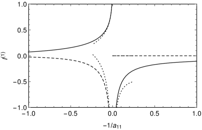
Figure 1: Functions ${\rm Re}I^{(1)}$ (solid) and ${\rm Im}I^{(1)}$ (dashed) characterizing the dependence of the effective three-body interaction on $a_{11}$ in one dimension [see Eqs. (58) and (40)]. $a_{11}$ is measured in units of $R_{\rm e}$. The dotted curves correspond to the large-$a_{11}$ asymptote [Eq. (62)]. For $a_{11}\rightarrow\pm 0$ one has $I^{(1)}\approx-0.03$.

Let us now discuss the function $I^{(1)}$. For large $a_{11}$ (weak atom-atom interaction) this function can be expanded in powers of $\sqrt{-1/a_{11}}$. In order to see this we rescale the momentum $p=\sqrt{-1/a_{11}}z$ and rewrite Eq. (59) in the form

$$\chi(z)=\frac{1}{1+z^{2}/2}$$

$$-\frac{1}{\sqrt{-a_{11}}}\frac{z^{2}}{1+z^{2}/2}\left[\frac{\sqrt{3}}{2}\sum_{\pm}\int\frac{\chi(y)}{z^{2}\pm yz+y^{2}}\frac{dy}{2\pi}+\frac{\chi(z)}{2|z|}\right],$$ (61)

which we then solve iteratively. In particular, the first iteration gives $\chi(z)=1/(1+z^{2}/2)$ and provides the leading order term $I^{(1)}\approx-\sqrt{-a_{11}/8}$. The second iteration results in

$$I^{(1)}=-\sqrt{-\frac{a_{11}}{8}}+\frac{9+5\sqrt{3}\pi+27\ln(-a_{11}e^{-2\gamma}/2)}{36\pi}+o(1).$$ (62)

The solid and dashed lines in Fig. 1 show, respectively, the real and imaginary parts of $I^{(1)}$ as a function of $-1/a_{11}$ ($=g_{11}/2$) obtained numerically. The dotted lines indicate the real and imaginary parts of the large-$a_{11}$ asymptote (62).

For negative $a_{11}$ the solution is real and ${\rm Im}I^{(1)}\equiv 0$. By contrast, for $a_{11}>0$ the function $\chi(p)$ is characterized by simple poles at $p=\pm(\kappa+i0)$, where $\kappa>0$ is defined by Eq. (24) [this is also the point where the term in round brackets in Eq. (59) vanishes]. These poles correspond to the three-body recombination to a dimer state, which, as found in Sec. III, exists only for positive $a_{11}$. One sees that $I^{(1)}$ and, therefore, $\tilde{f}(0)$ become complex reflecting the three-body loss. Technically, as one passes from positive to negative $-1/a_{11}$, the choice of the correct branch of the square root and logarithm in Eq. (62) is ensured by keeping $-1/a_{11}$ just below the real axis.

IV.2 Two dimensions

The solution in the two-dimensional case can be written as

$$\tilde{f}(0)=\frac{2\pi}{\ln(a_{12}e^{\gamma}/\sqrt{3})+2\pi I^{(2)}(a_{11})},$$ (63)

where $I^{(2)}(a_{11})=\int\frac{\chi(p)-1/(p^{2}+1)}{p^{2}}\frac{d^{2}p}{(2\pi)^{2}}$ and $\chi$ satisfies

$$\sum_{\pm}\int\frac{\chi(q)}{p^{2}\pm{\bf pq}+q^{2}}\frac{d^{2}q}{(2\pi)^{2}}+\left(\frac{1}{p^{2}}-\frac{1}{2\pi}\ln\frac{a_{11}pe^{\gamma}}{2}\right)\chi(p)=\frac{1}{p^{2}}.$$ (64)

The three-body scattering surface is proportional to $\tilde{f}(0)$ [see Eq. (42)] and the mean-field result (5) is recovered for weak attractive or repulsive atom-dimer interactions (small or large $a_{12}$). As in the one-dimensional case we see that the dependence on $a_{12}$ is analytic and for the complete solution of the problem one needs to know only $I^{(2)}(a_{11})$.

For a weak atom-atom background interaction (small or large $a_{11}$), introducing the small parameter $\lambda=1/\ln(1/a_{11})$, we can proceed iteratively in exactly the same manner as in the one-dimensional case. Namely, using the momentum rescaling $p=\sqrt{\lambda}z$ one can see that to the leading order $\chi(z)\approx 1/(1+z^{2}/2\pi)$ and after two iterations we have

$$I^{(2)}=\frac{\ln(2\pi\lambda)}{4\pi}+\lambda\frac{\ln(C\lambda)}{8\pi}+o(\lambda),$$ (65)

where $C\approx 0.013$.

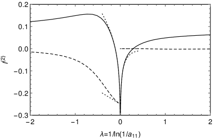
Figure 2: Real and imaginary parts of $I^{(2)}$ in the two-dimensional case. We use the same notations as in Fig. 1.

In Fig. 2 we plot the real (solid) and imaginary (dashed) parts of $I^{(2)}$ versus $\lambda$ together with the asymptote (65) (dotted). In the two-dimensional case ${\rm Im}I^{(2)}$ is always finite since there is always a dimer bound state available for the recombination (see Sec. III). However, for small positive $\lambda$ the dimer is exponentially deep and small (its energy is proportional to $1/a_{11}^{2}=e^{-1/\lambda}$) so that the recombination in this limit is not captured by the power expansion Eq. (65).

Note that for small $\lambda$ the characteristic momentum involved in the solution $\chi(p)$ is $\sqrt{\lambda}$. Therefore, the asymptotic expansion (65) is also valid if, instead of the zero-range atom-atom interaction, we have a potential of a finite but sufficiently small range $\ll 1/\sqrt{\lambda}=\sqrt{|\ln(1/a_{11})|}$, characterized by the same scattering length $a_{11}$. In particular, one can have a purely repulsive potential which does not lead to a dimer state in our problem.

IV.3 Three dimensions

In three dimensions we have

$$\tilde{f}(0)=\frac{1}{-\sqrt{3}/8\pi a_{12}+I^{(3)}(a_{11})},$$ (66)

where $I^{(3)}(a_{11})=\int\frac{\chi(p)}{p^{2}}\frac{d^{3}p}{(2\pi)^{3}}$ with $\chi$ satisfying

$$\frac{2}{\sqrt{3}}\sum_{\pm}\int\frac{\chi(q)}{p^{2}\pm{\bf pq}+q^{2}}\frac{d^{3}q}{(2\pi)^{3}}+\left(\frac{1}{p^{2}}-\frac{p}{4\pi}+\frac{1}{4\pi a_{11}}\right)\chi(p)=\frac{1}{p^{2}}.$$ (67)

Here we also manage to separate the dependencies on the atom-dimer and atom-atom interactions. The mean-field solution (5) is retrieved for $a_{12}\rightarrow 0$. Calculating $I^{(3)}$ is, however, more subtle than in the low-dimensional cases. Indeed, small hyperradii effectively correspond to high collision momenta and energies where the two-body scattering length is approximated by its background value $a_{11}$. Thus, at $\rho\ll a_{11}$ we deal with the Efimovian three-boson system which requires a three-body parameter or a cutoff momentum. Mathematically, this can be seen from Eq. (67) at momenta $p\gg 1/a_{11}$, where the dominant terms are the integral and $-p\chi(p)/4\pi$. The corresponding large-momentum behavior of $\chi(p)$ is a linear combination of Efimov waves $p^{\pm is_{0}-2}$ with $s_{0}\approx 1.00624$ Braaten2006 . The coefficients in this linear combination are fixed by introducing an external (three-body) parameter, phase, or momentum. Namely, one can set

$$\chi\propto\frac{\sin[s_{0}\ln(p/p_{0})]}{p^{2}}$$ (68)

as the asymptotic boundary condition for $p\gg 1/a_{11}$. Accordingly, the quantity $I^{(3)}$ is, in fact, a function of $a_{11}$ and the three-body parameter $p_{0}$. However, for small $a_{11}$ the leading-order contribution to $I^{(3)}$ is universal, i.e., independent of $p_{0}$. Indeed, for small $a_{11}$ and momenta $p\ll 1/|a_{11}|$ Eq. (67) reduces to $(1/p^{2}+1/4\pi a_{11})\chi(p)=1/p^{2}$. The corresponding solution $\chi=1/(1+p^{2}/4\pi a_{11})$ is characterized by the typical momentum $\sqrt{a_{11}}\ll 1/a_{11}$ and leads to

$$I^{(3)}\approx\sqrt{a_{11}/4\pi}.$$ (69)

In order to estimate the next-order term we match $\chi(p)$ with the Efimov wave (68) at momentum $p\sim 1/|a_{11}|$ obtaining a contribution to $I^{(3)}$ of the order of $a_{11}^{2}$.

It makes sense to study the case of larger $a_{11}$ ($\gtrsim R_{\rm e}$) within our zero-range model, if we deal with a zero crossing near a narrow Feshbach resonance (large $R_{\rm e}$) which, in turn, lies in the vicinity of a broader Feshbach resonance (large $a_{11}$). At the same time it is interesting to have a significant atom-dimer interaction (large $a_{12}$) such that the two terms in the denominator of Eq. (66) are comparable. Then, in order to find the effective three-body force we also need to know the three-body and inelasticity parameters (or, equivalently, the real and imaginary parts of $p_{0}$), which could be known from the Efimov loss spectroscopy near the broad resonance. Given the large number of parameters in this problem we just give a prescription for calculating $I^{(3)}$. Namely, one has to solve Eq. (67) with the boundary condition (68) at $p\rightarrow\infty$ also requiring $\chi\propto 1/(p-\kappa-i0)$ near the pole given by Eq. (26).

V Discussion and conclusions

In this article we have expanded the idea that the bosonic model with a Feshbach-type atom-dimer conversion (1) near a two-body zero crossing can be reduced to a purely atomic model with an effective three-body interaction, which strongly depends on the atom-dimer conversion amplitude. As a particular example, we show that this mechanism of generating three-body forces can be used for stabilizing supersolid phases of two-dimensional dipoles.

Sections III and IV have been devoted to constructing a zero-range regularized version of the model (1) with a minimal set of parameters ($a_{11}$, $a_{12}$, and $R_{\rm e}$). We have solved this model nonperturbatively in the two-body and three-body cases in all dimensions at the two-body zero crossing. Formulas (58), (63), and (66) give analytic dependencies of the three-body scattering amplitude on $a_{12}$ in different dimensions. The dependence on $a_{11}$ is found numerically and also analytically for weak atom-atom background interactions. In the three-dimensional case, our three-body zero-range model is Efimovian and requires an additional three-body parameter. We find, however, that for small $|a_{11}|/R_{\rm e}$, effects associated with the Efimov physics are subleading.

These results show that for comparable and weak atom-dimer and atom-atom interactions (characterized by $g_{12}$ and $g_{11}$, respectively), the three-body interaction is mostly influenced by $g_{12}$, consistent with the mean-field result (5). However, the convergence is not always uniform. For example, in the two-dimensional case, one can simultaneously decrease $g_{12}$ and $g_{11}$, keeping both terms in the denominator of Eq. (63) comparable to (or even canceling) each other (resulting in a diverging three-body scattering surface). In the same spirit, we can use the nonperturbative three-dimensional formula Eq. (66) and predict a three-body resonance at $\sqrt{3}R_{\rm e}/8\pi a_{12}\approx\sqrt{a_{11}/4\pi R_{\rm e}}\ll 1$.

Inelastic three-body events manifest themselves through the appearance of an imaginary part of $\tilde{f}(0)$, which, in turn, comes from the complex $I^{(D)}$ or complex atom-dimer scattering length $a_{12}$. The former reflects the three-body recombination to a dimer state and the latter the relaxation process in collisions of atoms with closed-channel dimers.

Several proposals on how to observe elastic three-body interactions experimentally are based on the following ideas. A repulsive three-body force could stabilize a system with attractive two-body interactions and make it self-trapped Bulgac2002 . The structure and energies of few-body bound states, detectable spectroscopically, are also influenced by these forces Sekino2018 ; Nishida2018 ; Pricoupenko2018 ; Guijarro2018 . Collective-mode frequency shifts in a trapped gas could be another experimentally observable signature of three-body interactions ValientePastukhov2019 .

References

- (1) H. Kadau, M. Schmitt, M. Wenzel, C. Wink, T. Maier, I. Ferrier-Barbut, and T. Pfau, Observing the Rosensweig instability of a quantum ferrofluid, Nature (London) 530, 194 (2016).
- (2) M. Schmitt, M. Wenzel, F. Böttcher, I. Ferrier-Barbut, and T. Pfau, Self-bound droplets of a dilute magnetic quantum liquid, Nature (London) 539, 259 (2016).
- (3) I. Ferrier-Barbut, H. Kadau, M. Schmitt, M. Wenzel, and T. Pfau, Observation of Quantum Droplets in a Strongly Dipolar Bose Gas, Phys. Rev. Lett. 116, 215301 (2016).
- (4) L. Chomaz, S. Baier, D. Petter, M. J. Mark, F. Wächtler, L. Santos, and F. Ferlaino, Quantum-Fluctuation-Driven Crossover from a Dilute Bose-Einstein Condensate to a Macrodroplet in a Dipolar Quantum Fluid, Phys. Rev. X 6, 041039 (2016).
- (5) C. R. Cabrera, L. Tanzi, J. Sanz, B. Naylor, P. Thomas, P. Cheiney, and L. Tarruell, Quantum liquid droplets in a mixture of Bose-Einstein condensates, Science 359, 301 (2017).
- (6) P. Cheiney, C. R. Cabrera, J. Sanz, B. Naylor, L. Tanzi, and L. Tarruell, Bright Soliton to Quantum Droplet Transition in a Mixture of Bose-Einstein Condensates, Phys. Rev. Lett. 120, 135301 (2018).
- (7) G. Semeghini, G. Ferioli, L. Masi, C. Mazzinghi, L. Wolswijk, F. Minardi, M. Modugno, G. Modugno, M. Inguscio, and M. Fattori, Self-Bound Quantum Droplets of Atomic Mixtures in Free Space, Phys. Rev. Lett. 120, 235301 (2018).
- (8) D. S. Petrov, Quantum mechanical stabilization of a collapsing Bose-Bose mixture, Phys. Rev. Lett. 115, 155302 (2015).
- (9) F. Wächtler and L. Santos, Quantum filaments in dipolar Bose-Einstein condensates, Phys. Rev. A 93, 061603(R) (2016).
- (10) R. N. Bisset, R. M. Wilson, D. Baillie, and P. B. Blakie, Ground-state phase diagram of a dipolar condensate with quantum fluctuations, Phys. Rev. A 94, 033619 (2016).
- (11) L. Tanzi, E. Lucioni, F. Famà, J. Catani, A. Fioretti, C. Gabanini, R. N. Bisset, L. Santos, and G. Modugno, Observation of a Dipolar Quantum Gas with Metastable Supersolid Properties, Phys. Rev. Lett. 122, 130405 (2019).
- (12) L. Chomaz, D. Petter, P. Ilzhöfer, G. Natale, A. Trautmann, C. Politi, G. Durastante, R. M. W. van Bijnen, A. Patscheider, M. Sohmen, M. J. Mark, and F. Ferlaino, Long-Lived and Transient Supersolid Behaviors in Dipolar Quantum Gases, Phys. Rev. X 9, 021012 (2019).
- (13) F. Böttcher, J.-N. Schmidt, M. Wenzel, J. Hertkorn, M. Guo, T. Langen, and T. Pfau, Transient Supersolid Properties in an Array of Dipolar Quantum Droplets, Phys. Rev. X 9, 011051 (2019).
- (14) L. Tanzi, S. M. Roccuzzo, E. Lucioni, F. Famà, A. Fioretti, C. Gabbanini, G. Modugno, A. Recati, and S. Stringari, Supersolid symmetry breaking from compressional oscillations in a dipolar quantum gas, Nature (London) (2019) doi:10.1038/s41586-019-1568-6.
- (15) M. Guo, F. Böttcher, J. Hertkorn, J.-N. Schmidt, M. Wenzel, H.-P. Büchler, T. Langen, and T. Pfau, The low-energy Goldstone mode in a trapped dipolar supersolid, Nature (London) (2019) doi:10.1038/s41586-019-1569-5.
- (16) A. Bulgac, Dilute Quantum Droplets, Phys. Rev. Lett. 89, 050402 (2002).
- (17) D. S. Petrov, Three-Body Interacting Bosons in Free Space, Phys. Rev. Lett. 112, 103201 (2014).
- (18) K.-T. Xi and H. Saito, Droplet formation in a Bose-Einstein condensate with strong dipole-dipole interaction, Phys. Rev. A 93, 011604(R) (2016).
- (19) R. N. Bisset and P. B. Blakie, Crystallization of a dilute atomic dipolar condensate, Phys. Rev. A 92, 061603(R) (2015).
- (20) Z.-K. Lu, Y. Li, D. S. Petrov, and G. V. Shlyapnikov, Stable dilute supersolid of two-dimensional dipolar bosons, Phys. Rev. Lett. 115, 075303 (2015).
- (21) A. Pricoupenko and D. S. Petrov, Dimer-dimer zero crossing and dilute dimerized liquid in a one-dimensional mixture, Phys. Rev. A. 97, 063616 (2018).
- (22) Y. Sekino and Y. Nishida, Quantum droplet of one-dimensional bosons with a three-body attraction, Phys. Rev. A 97, 011602(R) (2018).
- (23) J. E. Drut, J. R. McKenney, W. S. Daza, C. L. Lin, and C. R. Ordóñez, Quantum Anomaly and Thermodynamics of One-Dimensional Fermions with Three-Body Interactions, Phys. Rev. Lett. 120, 243002 (2018).
- (24) Y. Nishida, Universal bound states of one-dimensional bosons with two- and three-body attractions, Phys. Rev. A 97, 061603 (2018).
- (25) L. Pricoupenko, Pure confinement-induced trimer in one-dimensional atomic waveguides, Phys. Rev. A 97, 061604 (2018).
- (26) G. Guijarro, A. Pricoupenko, G. E. Astrakharchik, J. Boronat, and D. S. Petrov, One-dimensional three-boson problem with two- and three-body interactions, Phys. Rev. A. 97, 061605(R) (2018).
- (27) L. Pricoupenko, Three-body pseudopotential for atoms confined in one dimension, Phys. Rev. A 99, 012711 (2018).
- (28) W. S. Daza, J. E. Drut, C. L. Lin, C. R. Ordóñez, A Quantum Field-Theoretical Perspective on Scale Anomalies in 1D systems with Three-Body Interactions, Mod. Phys. Lett. A 34, 1950291 (2019).
- (29) J. R. McKenney and J. E. Drut, Fermi-Fermi crossover in the ground state of one-dimensional few-body systems with anomalous three-body interactions, Phys. Rev. A 99, 013615 (2019).
- (30) V. Pastukhov, Ground-state properties of dilute one-dimensional Bose gas with three-body repulsion, Phys. Lett. A 383, 894 (2019).
- (31) M. Valiente, Three-body repulsive forces among identical bosons in one dimension, Phys. Rev. A 100, 013614 (2019).
- (32) M. Valiente and V. Pastukhov, Anomalous frequency shifts in a one-dimensional trapped Bose gas, Phys. Rev. A 99, 053607 (2019).
- (33) L. Radzihovsky, P. B. Weichman, and J. I. Park, Superfluidity and phase transitions in a resonant Bose gas, Ann. Phys. 323, 2376 (2008).
- (34) M. A. Baranov, A. Micheli, S. Ronen, and P. Zoller, Bilayer superfluidity of fermionic polar molecules: Many-body effects, Phys. Rev. A 83, 043602 (2011).
- (35) Z. Shotan, O. Machtey, S. Kokkelmans, and L. Khaykovich, Three-Body Recombination at Vanishing Scattering Lengths in an Ultracold Bose Gas, Phys. Rev. Lett. 113, 053202 (2014).
- (36) G. Quéméner and J. L. Bohn, Electric field suppression of ultracold confined chemical reactions, Phys. Rev. A 81, 060701(R) (2010).
- (37) A. Micheli, Z. Idziaszek, G. Pupillo, M. A. Baranov, P. Zoller, and P. S. Julienne, Universal Rates for Reactive Ultracold Polar Molecules in Reduced Dimensions, Phys. Rev. Lett. 105, 073202 (2010).
- (38) A. Frisch, M. Mark, K. Aikawa, S. Baier, R. Grimm, A. Petrov, S. Kotochigova, G. Quéméner, M. Lepers, O. Dulieu, and F. Ferlaino, Ultracold Dipolar Molecules Composed of Strongly Magnetic Atoms, Phys. Rev. Lett. 115, 203201 (2015).
- (39) R. Stock, A. Silberfarb, E. L. Bolda, and I. H. Deutsch, Generalized Pseudopotentials for Higher Partial Wave Scattering, Phys. Rev. Lett. 94, 023202 (2005).
- (40) K. Kanjilal and D. Blume, Coupled-channel pseudopotential description of the Feshbach resonance in two dimensions, Phys. Rev. A 73, 060701(R) (2006).
- (41) D. S. Petrov, in Proceedings of the Les Houches Summer Schools, Session 94, edited by C. Salomon, G. V. Shlyapnikov, and L. F. Cugliandolo (Oxford University Press, Oxford, England, 2013).
- (42) The prefactor here [and also in Eqs. (36), (47-49)] comes from our definition of the Jacobi coordinates (28), according to which the atom-dimer distance equals .
- (43) See, for example, page 359 in E. Braaten and H.-W. Hammer, Universality in few-body systems with large scattering length, Phys. Rep. 428, 259 (2006).