Dimensional Reweighting Graph Convolutional Networks

Abstract

In this paper, we propose a method named Dimensional reweighting Graph Convolutional Networks (DrGCNs), to tackle the problem of variance between dimensional information in the node representations of GCNs. We prove that DrGCNs have the effect of stabilizing the training process by connecting our problem to the theory of the mean field. However, practically, we find that the degrees DrGCNs help vary severely on different datasets. We revisit the problem and develop a new measure $K$ to quantify the effect. This measure guides when we should use dimensional reweighting in GCNs and how much it can help. Moreover, it offers insights to explain the improvement obtained by the proposed DrGCNs. The dimensional reweighting block is light-weighted and highly flexible to be built on most of the GCN variants. Carefully designed experiments, including several fixes on duplicates, information leaks, and wrong labels of the well-known node classification benchmark datasets, demonstrate the superior performances of DrGCNs over the existing state-of-the-art approaches. Significant improvements can also be observed on a large scale industrial dataset.

1 Introduction

Deep neural networks (DNNs) have been widely applied in various fields, including computer vision  (he2016deep; hu2018squeeze), natural language processing  (devlin2018bert), and speech recognition  (abdel2014convolutional), among many others. Graph neural networks (GNNs) is proposed for learning node presentations of networked data (scarselli2009graph), and later be extended to graph convolutional network (GCN) that achieves better performance by capturing topological information of linked graphs (kipf2017semi). Since then, GCNs begin to attract board interests. Starting from GraphSAGE (hamilton2017inductive) defining the convolutional neural network based graph learning framework as sampling and aggregation, many follow-up efforts attempt to enhance the sampling or aggregation process via various techniques, such as attention mechanism (velivckovic2018graph), mix-hop connection (abu2019mixhop) and adaptive sampling (huang2018adaptive).

In this paper, we study the node representations in GCNs from the perspective of covariance between dimensions. Suprisingly, applying a dimensional reweighting process to the node representations may be very useful for the improvement of GCNs. As an instance, under our proposed reweighting scheme, the input covariance between dimensions can be reduced by 68% on the Reddit dataset, which is extremely useful since we also find that the number of misclassified cases reduced by 40%, compared with the previous SOTA method.

We propose Dimensional reweighting Graph Convolutional Networks (DrGCNs), in which the input of each layer of the GCN is reweighted by global node representation information. Our discovery is that the experimental performance of GCNs can be greatly improved under this simple reweighting scheme. On the other hand, with the help of mean field theory (kadanoff2009more; yang2019mean), this reweighting scheme is also proved to improve the stability of fully connected networks, provding insight to GCNs. To deepen the understanding to which extent the proposed reweighting scheme can help GCNs, we develop a new measure to quantify its effectiveness under different contexts (GCN variants and datasets).

Experimental results verify our theoretical findings ideally that we can achieve predictable improvements on public datasets adopted in the literature over the state-of-the-art GCNs. While studying on these well-known benchmarks, we notice that two of them (Cora, Citeseer) suffer from duplicates and feature-label information leaks. We fix these problems and offer refined datasets for fair comparisons. To further validate the effectiveness, we deploy the proposed DrGCNs on A* company’s recommendation system and clearly demonstrate performance improvements via offline evaluations.

2 DrGCNs: Dimensional reweighting Graph Convolutional Networks

2.1 Preliminaries

Notations. We focus on undirected graphs $\mathcal{G}=(\mathcal{V},\mathcal{E},\mathbf{X})$, where $\mathcal{V}=\{v_{i}\}$ represents the node set, $\mathcal{E}=\{(v_{i},v_{j})\}$ indicates the edge set, and $\mathbf{X}$ stands for the node features. For a specific GCN layer, we use $\mathbf{R}^{in}=(\mathbf{r}^{in}_{1},...,\mathbf{r}^{in}_{n})$ to denote the input node representations and $\mathbf{R}^{out}=(\mathbf{r}^{out}_{1},...,\mathbf{r}^{out}_{n})$ to symbolize the output representations. For the whole layer-stacked GCN structure, we use $\mathbf{H}^{0}$ to denote the input node representation of the first layer, and $\mathbf{H}^{l}(l>0)$ to signify the output node representation of the $l^{th}$ layer, which is also the output representation of the $(l-1)^{th}$ layer. Let $\mathbf{A}$ be the adjacency matrix with $a_{ij}=1$ when $(v_{i},v_{j})\in\mathcal{E}$ and $a_{ij}=0$ otherwise.

Graph Convolutional Networks (GCNs). Given the input node set $\mathcal{V}$, the adjacency matrix $\mathbf{A}$, and the input representations $\mathbf{R}^{in}$, a GCN layer uses such information to generate output representations $\mathbf{R}^{out}$:

$$\mathbf{R}^{out}=\sigma(aggregator(\mathbf{R}^{in},\mathbf{A})),$$ (1)

where $\sigma$ is the activation function. Although there exist non-linear aggregators like the LSTM aggregator (hamilton2017inductive), in most GCN variants the aggregator is a linear function which can be viewed as a weighted sum of node representations among the neighborhood (kipf2017semi; huang2018adaptive), followed by a matrix multiplication on a refined adjacency matrix $\mathbf{\tilde{A}}$, with a bias added. The procedure can be formulated as follows:

$$\mathbf{R}^{out}=\sigma(\mathbf{W}\mathbf{R}^{in}\mathbf{\tilde{A}}+\mathbf{b}),$$ (2)

where $\mathbf{W}$ is the projection matrix and $\mathbf{b}$ denotes the bias vector. Development on GCNs mainly lies in different ways to generate $\mathbf{\tilde{A}}$. GCN proposed some variants including simply taking $\mathbf{\tilde{A}}=\mathbf{A}\mathbf{D}^{-1}$, which is uniform average among neighbors with $\mathbf{D}$ being the diagonal matrix of the degrees, or weighted by degree of each node $\mathbf{\tilde{A}}=\mathbf{D}^{-\frac{1}{2}}\mathbf{A}\mathbf{D}^{-\frac{1}{2}}$, or including self-loops $\mathbf{\tilde{A}}=\mathbf{I}+\mathbf{D}^{-\frac{1}{2}}\mathbf{A}\mathbf{D}^{-\frac{1}{2}}$. Other methods include attention  (velivckovic2018graph), or gated attention  (zhang2018gaan), or even neural architecture search methods (gao2019graphnas) to generate $\mathbf{\tilde{A}}$. To improve scalability, some GCN variants contain a sampling procedure, which samples a subset of the neighborhood for aggregation  (chen2018fastgcn; huang2018adaptive). We can set all unsampled edges to 0 in $\mathbf{\tilde{A}}$ in sampling-based GCNs, in this case $\mathbf{\tilde{A}}$ even has some randomness.

2.2 Model Formulation for DrGCNs

Given input node representations of a GCN layer $\mathbf{R}^{in}$, the proposed DrGCN tries to learn a dimensional reweighting vector $\mathbf{s}=(s_{1},...,s_{d})$, where $s_{i}$ is an adaptive scalar for each dimension $i$. This reweighting vector $\mathbf{s}$ then helps reweighting each dimension of the node representation $\mathbf{r}_{v}^{in}$ to $\mathbf{r}^{re}_{v}$, $v\in\mathcal{V}$, where $\mathbf{r}^{re}_{v}=\mathbf{r}^{in}_{v}\circ\mathbf{s}$. Here we use $\circ$ to denote component-wise multiplication, i.e.,

$$r^{re}_{v,j}=s_{j}r^{in}_{v,j},\forall 1\leq j\leq d,\forall v\in\mathcal{V}.$$ (3)

We define $\mathbf{S}$ as the diagonal matrix with diagonal entries corresponding to the components of $\mathbf{s}$. Then a DrGCN layer can be formulated as:

$$\mathbf{R}^{out}=\sigma(\mathbf{W}\mathbf{S}\mathbf{R}^{in}\mathbf{\tilde{A}}+\mathbf{b}).$$ (4)

Inspired by SENet (hu2018squeeze), we formulate the learning of the shared dimensional reweighting vector $\mathbf{s}$ in two stages. First we generate a global representation $\mathbf{r}^{in}$, whose value is the expectation of $\mathbf{r}_{v}^{in}$ on the whole graph. Then we feed $\mathbf{r}^{in}$ into a two-layer neural network structure to generate $\mathbf{s}$ of the same dimension size. Equation (5) denotes the procedure to generate $\mathbf{s}$ given node weight $\{w_{v}|v\in\mathcal{V},\sum_{v\in\mathcal{V}}w_{v}=1\}$ and node representations $\{\mathbf{r}^{in}_{v}|v\in\mathcal{V}\}$:

$$\centering\begin{split}\mathbf{r}^{in}=&E[\mathbf{r}^{in}_{v}|v\in\mathcal{V}]=\sum_{v\in\mathcal{V}}w_{v}\mathbf{r}^{in}_{v},\\ &\mathbf{g}=\sigma_{g}(\mathbf{W}_{g}\mathbf{r}^{in}+\textbf{b}_{g}),\\ &\mathbf{s}=\sigma_{s}(\mathbf{W}_{s}\mathbf{g}+\textbf{b}_{s}),\end{split}\@add@centering$$ (5)

where $\mathbf{g}$ is output of the first layer; $\mathbf{W}_{g},\mathbf{b}_{g},\mathbf{W}_{s},$ and $\mathbf{b}_{s}$ are parameters to be learnt. Figure 1 summarizes the dimensional reweighting block (Dr Block) in DrGCNs.

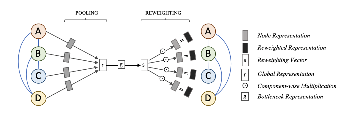
Figure 1: Our proposed dimensional reweighting block (Dr Block) in DrGCNs.

Combining With Existing GCN variants. The proposed Dr Block can be implemented as an independent functional process and easily combined with GCNs. As shown in equation (4), Dr Block only applies on $\mathbf{R}^{in}$ and does not involve in the calculation of $\mathbf{\tilde{A}},\mathbf{W}$ and $\mathbf{b}$. Hence, the proposed Dr Block can easily be combined with existing sampling or aggregation methods without causing any contradictions. In § LABEL:sec:exp, we will experimentally test the combination of our Dr Block with different types of sample-and-aggregation GCN methods. Suppose that the input features are $\mathbf{X}$, DrGCNs can be viewed as follows:

$$\mathbf{H}^{l}=\sigma_{l}(\mathbf{W}^{l}\mathbf{S}^{l}\mathbf{H}^{l-1}\mathbf{\tilde{A}}^{l}+\mathbf{b}^{l}),\forall 1\leq l\leq k,$$ (6)

where $\mathbf{H}^{0}=\mathbf{X}$ and $\mathbf{H}^{k}$ being the output representation for a $k$-layer DrGCN:

Complexity of Dr Block. Consider a GCN layer with $a$ input and $b$ output channels, $n$ nodes and $e$ edges in a sampled batch, the complexity of a GCN layer is $O(abn+be)$. The proposed Dr block has a complexity of $O(ag)$, where $g$ is the dimension of $\mathbf{g}$. In most cases, we have $g<b$ and $n>>1$, so we could have $O(ag)=o(abn+be)$, which indicates that Dr block introduces negligible extra computational cost.

3 Theoretical Analyses

In this section, we connect our study to mean field theory  (yang2019mean). We theoretically prove that the proposed Dr Block is capable of reducing the learning variance brought by perturbations on the input, making the update more stable in the long run. To deepen the understanding, we further develop a measure to quantify the stability gained by Dr block.

3.1 Mean Field Approximation