Graph Representation Learning via Hard and Channel-Wise Attention Networks

Abstract.

Attention operators have been widely applied in various fields, including computer vision, natural language processing, and network embedding learning. Attention operators on graph data enables learnable weights when aggregating information from neighboring nodes. However, graph attention operators (GAOs) consume excessive computational resources, preventing their applications on large graphs. In addition, GAOs belong to the family of soft attention, instead of hard attention, which has been shown to yield better performance. In this work, we propose novel hard graph attention operator (hGAO) and channel-wise graph attention operator (cGAO). hGAO uses the hard attention mechanism by attending to only important nodes. Compared to GAO, hGAO improves performance and saves computational cost by only attending to important nodes. To further reduce the requirements on computational resources, we propose the cGAO that performs attention operations along channels. cGAO avoids the dependency on the adjacency matrix, leading to dramatic reductions in computational resource requirements. Experimental results demonstrate that our proposed deep models with the new operators achieve consistently better performance. Comparison results also indicates that hGAO achieves significantly better performance than GAO on both node and graph embedding tasks. Efficiency comparison shows that our cGAO leads to dramatic savings in computational resources, making them applicable to large graphs.

1. Introduction

Deep attention networks are becoming increasingly powerful in solving challenging tasks in various fields, including natural language processing (Vaswani et al., 2017; Luong et al., 2015; Devlin et al., 2018), and computer vision (Wang et al., 2018; Xu et al., 2015; Zhao et al., 2018). Compared to convolution layers and recurrent neural layers like LSTM (Hochreiter and Schmidhuber, 1997; Gregor et al., 2015), attention operators are able to capture long-range dependencies and relationships among input elements, thereby boosting performance (Devlin et al., 2018; Li et al., 2018). In addition to images and texts, attention operators are also applied on graphs (Veličković et al., 2017). In graph attention operators (GAOs), each node in a graph attend to all neighboring nodes, including itself. By employing attention mechanism, GAOs enable learnable weights for neighboring feature vectors when aggregating information from neighbors. However, a practical challenge of using GAOs on graph data is that they consume excessive computational resources, including computational cost and memory usage. The time and space complexities of GAOs are both quadratic to the number of nodes in graphs. At the same time, GAOs belong to the family of soft attention (Jaderberg et al., 2015), instead of hard attention (Xu et al., 2015). It has been shown that hard attention usually achieves better performance than soft attention, since hard attention only attends to important features (Shankar et al., 2018; Xu et al., 2015; Yu et al., 2019).

In this work, we propose novel hard graph attention operator (hGAO). hGAO performs attention operation by requiring each query node to only attend to part of neighboring nodes in graphs. By employing a trainable project vector $\boldsymbol{p}$, we compute a scalar projection value of each node in graph on $\boldsymbol{p}$. Based on these projection values, hGAO selects several important neighboring nodes to which the query node attends. By attending to the most important nodes, the responses of the query node are more accurate, thereby leading to better performance than methods based on soft attention. Compared to GAO, hGAO also saves computational cost by reducing the number of nodes to attend.

GAO also suffers from the limitations of excessive requirements on computational resources, including computational cost and memory usage. hGAO improves the performance of attention operator by using hard attention mechanism. It still consumes large amount of memory, which is critical when learning from large graphs. To overcome this limitation, we propose a novel channel-wise graph attention operator (cGAO). cGAO performs attention operation from the perspective of channels. The response of each channel is computed by attending to all channels. Given that the number of channels is far smaller than the number of nodes, cGAO can significantly save computational resources. Another advantage of cGAO over GAO and hGAO is that it does not rely on the adjacency matrix. In both GAO and hGAO, the adjacency matrix is used to identify neighboring nodes for attention operators. In cGAO, features within the same node communicate with each other, but features in different nodes do not. cHAO does not need the adjacency matrix to identify nodes connectivity. By avoiding dependency on the adjacency matrix, cGAO achieves better computational efficiency than GAO and hGAO.

Based on our proposed hGAO and cGAO, we develop deep attention networks for graph embedding learning. Experimental results on graph classification and node classification tasks demonstrate that our proposed deep models with the new operators achieve consistently better performance. Comparison results also indicates that hGAO achieves significantly better performance than GAOs on both node and graph embedding tasks. Efficiency comparison shows that our cGAO leads to dramatic savings in computational resources, making them applicable to large graphs.

2. Background and Related Work

In this section, we describe the attention operator and related hard attention and graph attention operators.

2.1. Attention Operator

An attention operator takes three matrices as input; those are a query matrix $\boldsymbol{Q}=[\mathbf{q}_{1},\mathbf{q}_{2},\cdots,\mathbf{q}_{m}]\in\mathbb{R}^{d\times m}$ with each $\mathbf{q}_{i}\in\mathbb{R}^{d}$, a key matrix $\boldsymbol{K}=[\mathbf{k}_{1},\mathbf{k}_{2},\cdots,\mathbf{k}_{n}]\in\mathbb{R}^{d\times n}$ with each $\mathbf{k}_{i}\in\mathbb{R}^{d}$, and a value matrix $\boldsymbol{V}=[\mathbf{v}_{1},\mathbf{v}_{2},\cdots,\mathbf{v}_{n}]\in\mathbb{R}^{p\times n}$ with each $\mathbf{v}_{i}\in\mathbb{R}^{p}$. For each query vector $\boldsymbol{q}_{i}$, the attention operator produces its response by attending it to every key vector in $\boldsymbol{K}$. The results are used to compute a weighted sum of all value vectors in $\boldsymbol{V}$, leading to the output of the attention operator. The layer-wise forward-propagation operation of attn($\boldsymbol{Q}$, $\boldsymbol{K}$, $\boldsymbol{V}$) is defined as

(1) $$\boldsymbol{E} =\boldsymbol{K}^{T}\boldsymbol{Q} \in \mathbb{R}^{n\times m},$$

$$\boldsymbol{O} =\boldsymbol{V}\mbox{softmax}(\boldsymbol{E}) \in \mathbb{R}^{p\times m},$$

where $\mbox{softmax}(\cdot)$ is a column-wise softmax operator.

The coefficient matrix $\boldsymbol{E}$ is calculated by the matrix multiplication between $\boldsymbol{K}^{T}$ and $\boldsymbol{Q}$. Each element $e_{ij}$ in $\boldsymbol{E}$ represents the inner product result between the key vector $\boldsymbol{k}^{T}_{i}$ and the query vector $\boldsymbol{q}_{j}$. The matrix multiplication $\boldsymbol{K}^{T}\boldsymbol{Q}$ computes all similarity scores between all query vectors and all key vectors. The column-wise softmax operator is used to normalize the coefficient matrix and make the sum of each column to 1. The matrix multiplication between $\boldsymbol{V}$ and $\mbox{softmax}(\boldsymbol{E})$ produces the output $\boldsymbol{O}$. Self-attention  (Vaswani et al., 2017) is a special attention operator with $\boldsymbol{Q}=\boldsymbol{K}=\boldsymbol{V}$.

In Eq. 1, we employ dot product to calculate responses between query vectors in $\boldsymbol{Q}$ and key vectors in $\boldsymbol{K}$. There are several other ways to perform this computation, such as Gaussian function and concatenation. Dot product is shown to be the simplest but most effective one (Wang et al., 2018). In this work, we use dot product as the similarity function. In general, we can apply linear transformations on input matrices, leading to following attention operator:

(2) $$\boldsymbol{E} =(\boldsymbol{W}^{K}\boldsymbol{K})^{T}\boldsymbol{W}^{Q}\boldsymbol{Q} \in \mathbb{R}^{n\times m},$$

$$\boldsymbol{O} =\boldsymbol{W}^{V}\boldsymbol{V}\mbox{softmax}(\boldsymbol{E}) \in \mathbb{R}^{p^{\prime}\times m},$$

where $\boldsymbol{W}^{V}\in\mathbb{R}^{p^{\prime}\times p}$ $\boldsymbol{W}^{K}\in\mathbb{R}^{d^{\prime}\times d}$ and $\boldsymbol{W}^{Q}\in\mathbb{R}^{d^{\prime}\times d}$. In the following discussions, we will skip linear transformations for the sake of notational simplicity.

The computational cost of the attention operator as described in Eq. 1 is $O(n\times d\times m)+O(p\times n\times m)=O(n\times m\times(d+p))$. The space complexity for storing intermediate coefficient matrix $\boldsymbol{E}$ is $O(n\times m)$. If $d=p$ and $m=n$, the time and space complexities are $O(m^{2}\times d)$ and $O(m^{2})$, respectively.

2.2. Hard Attention Operator

The attention operator described above uses soft attention, since responses to each query vector $\boldsymbol{q}_{i}$ are calculated by taking weighted sum over all value vectors. In contrast, hard attention operator (Xu et al., 2015) only selects a subset of key and value vectors for computation. Suppose $k$ key vectors ($k<n$) are selected from the input matrix $\boldsymbol{K}$ and the indices are $i_{1},i_{2},\cdots,i_{k}$ with $i_{m}<i_{n}$ and $1\leq m<n\leq k$. With selected indices, new key and value matrices are constructed as $\boldsymbol{\tilde{K}}=[\mathbf{k}_{i_{1}},\mathbf{k}_{i_{2}},\ldots,\mathbf{k}_{i_{k}}]\in\mathbb{R}^{d\times k}$ and $\boldsymbol{\tilde{V}}=[\mathbf{v}_{i_{1}},\mathbf{v}_{i_{2}},\ldots,\mathbf{v}_{i_{k}}]\in\mathbb{R}^{p\times k}$. The output of the hard attention operator is obtained by $\boldsymbol{O}=\mbox{attn}(\boldsymbol{Q},\boldsymbol{\tilde{K}},\boldsymbol{\tilde{V}})$. The hard attention operator is converted into a stochastic process in (Xu et al., 2015) by setting $k$ to 1 and use probabilistic sampling. For each query vector, it only selects one value vector by probabilistic sampling based on normalized similarity scores given by $\mbox{softmax}(\boldsymbol{K}\boldsymbol{q}_{i})$. The hard attention operators using probabilistic sampling are not differentiable, and requires reinforcement learning techniques for training. This makes soft attention more popular for easier back-propagation training (Ling and Rush, 2017).

By attending to less key vectors, the hard attention operator is computationally more efficient than the soft attention operator. The time and space complexities of the hard attention operator are $O(m\times k\times d)$ and $O(m\times k)$, respectively. When $k\ll m$, the hard attention operator reduces time and space complexities by a factor of $m$ compared to the soft attention operator. Besides computational efficiency, the hard attention operator is shown to have better performance than the soft attention operator (Xu et al., 2015; Luong et al., 2015), because it only selects important feature vectors to attend (Malinowski et al., 2018; Juefei-Xu et al., 2016).

2.3. Graph Attention Operator

The graph attention operator (GAO) was proposed in (Veličković et al., 2017), and it applies the soft attention operator on graph data. For each node in a graph, it attends to its neighboring nodes. Given a graph with $N$ nodes, each with $d$ features, the layer-wise forward propagation operation of GAO in (Veličković et al., 2017) is defined as

(3) $$\boldsymbol{\tilde{E}} =(\boldsymbol{X}^{T}\boldsymbol{X})\circ\boldsymbol{A},$$

$$\boldsymbol{O} =\boldsymbol{X}\mbox{softmax}(\boldsymbol{\tilde{E}}),$$

where $\circ$ denotes element-wise matrix multiplication, $\boldsymbol{A}\in\{0,1\}^{N\times N}$ and $\boldsymbol{X}=[\boldsymbol{x}_{1},\boldsymbol{x}_{2},\ldots,\boldsymbol{x}_{N}]\in\mathbb{R}^{d\times N}$ are the adjacency and feature matrices of a graph. Each $\boldsymbol{x}_{i}\in\mathbb{R}^{d}$ is node $i$’s feature vector. In some situations, $\boldsymbol{A}$ can be normalized as needed (Kipf and Welling, 2017). Note that the softmax function only applies to nonzero elements of $\boldsymbol{\tilde{E}}$.

The time complexity of GAO is $O(Cd)$, where $C$ is the number of edges. On a dense graph with $C\approx N^{2}$, this reduces to $O(N^{2}d)$. On a sparse graph, sparse matrix operations are required to compute GAO with this efficiency. However, current tensor manipulation frameworks such as TensorFlow do not support efficient batch training with sparse matrix operations (Veličković et al., 2017), making it hard to achieve this efficiency. In general, GAO consumes excessive computational resources, preventing its applications on large graphs.

3. Hard and Channel-Wise Attention Operators and Networks

In this section, we describe our proposed hard graph attention operator (hGAO) and channel-wise graph attention operator (cGAO). hGAO applies the hard attention operation on graph data, thereby saving computational cost and improving performance. cGAO performs attention operation on channels, which avoids the dependency on the adjacency matrix and significantly improves efficiency in terms of computational resources. Based on these operators, we propose the deep graph attention networks for network embedding learning.

3.1. Hard Graph Attention Operator

Graph attention operator (GAO) consumes excessive computation resources, including computational cost and memory usage, when graphs have a large number of nodes, which is very common in real-world applications. Given a graph with $N$ nodes, each with $d$ features, GAO requires $O(N^{2}d)$ and $O(N^{2})$ time and space complexities to compute its outputs. This means the computation cost and memory required grow quadratically in terms of graph size. This prohibits the application of GAO on graphs with a large number of nodes. In addition, GAO uses the soft attention mechanism, which computes responses of each node from all neighboring nodes in the graph. Using hard attention operator to replace the soft attention operator can reduce computational cost and improve learning performance. However, there is still no hard attention operator on graph data to the best of our knowledge. Direct use of the hard attention operator as in (Xu et al., 2015) on graph data still incurs excessive computational resources. It requires the computation of the normalized similarity scores for probabilistic sampling, which is the key factor of high requirements on computational resources.

To address the above limitations of GAO, we propose the hard graph attention operator (hGAO) that applies hard attention on graph data to save computational resources. For all nodes in a graph, we use a projection vector $\boldsymbol{p}\in\mathbb{R}^{d}$ to select the $k$-most important nodes to attend. Following the notations defined in Section 2, the layer-wise forward propagation function of hGAO is defined as

(4) $$\boldsymbol{y}=\frac{|\boldsymbol{X}^{T}\boldsymbol{p}|}{\lVert\boldsymbol{p}\rVert} \in \mathbb{R}^{N}$$

$$\mbox{for }i=1,2,\cdots,N\mbox{ do}$$

(5) $$\,\,\,\,\,\,\,\,\boldsymbol{idx}_{i}=\mbox{Ranking}_{k}(\boldsymbol{A_{:i}}\circ\boldsymbol{y}) \in \mathbb{R}^{k}$$

(6) $$\,\,\,\,\,\,\,\,\boldsymbol{\hat{X}}_{i}=\boldsymbol{X}(:,\boldsymbol{idx}_{i}) \in \mathbb{R}^{d\times k}$$

(7) $$\,\,\,\,\,\,\,\,\boldsymbol{\tilde{y}}_{i}=\mbox{sigmoid}(\boldsymbol{y}(\boldsymbol{idx}_{i})) \in \mathbb{R}^{k}$$

(8) $$\,\,\,\,\,\,\,\,\boldsymbol{\tilde{X}}_{i}=\boldsymbol{\hat{X}}_{i}\mbox{diag}(\boldsymbol{\tilde{y}}_{i}) \in \mathbb{R}^{d\times k}$$

(9) $$\,\,\,\,\,\,\,\,\boldsymbol{z}_{i}=\mbox{attn}(\boldsymbol{x}_{i},\boldsymbol{\tilde{X}}_{i},\boldsymbol{\tilde{X}}_{i}) \in \mathbb{R}^{d}$$

(10) $$\boldsymbol{Z}=[\boldsymbol{z}_{1},\boldsymbol{z}_{2},\ldots,\boldsymbol{z}_{N}] \in \mathbb{R}^{d\times N}$$

where $\boldsymbol{A_{:i}}$ denotes the $i$th column of matrix $\boldsymbol{A}$, $\boldsymbol{X}(:,\boldsymbol{idx}_{i})$ contains a subset of columns of $\boldsymbol{X}$ indexed by $\boldsymbol{idx}_{i}$, $|\cdot|$ computes element-wise absolute values, $\circ$ denotes element-wise matrix/vector multiplication, $\mbox{diag}(\cdot)$ constructs a diagonal matrix with the input vector as diagonal elements, $\mbox{Ranking}_{k}(\cdot)$ is an operator that performs the $k$-most important nodes selection for the query node $i$ to attend and is described in detail below.

We propose a novel node selection method in hard attention. For each node in the graph, we adaptively select the $k$ most important adjacent nodes. By using a trainable projection vector $\boldsymbol{p}$, we compute the absolute scalar projection of $\boldsymbol{X}$ on $\boldsymbol{p}$ in Eq. (4), resulting in $\boldsymbol{y}=[y_{1},y_{2},\cdots,y_{N}]^{T}$. Here, each $y_{i}$ measures the importance of node $i$. For each node $i$, the $\mbox{Ranking}_{k}(\cdot)$ operation in Eq. (5) ranks node $i$’s adjacent nodes by their projection values in $\boldsymbol{y}$, and selects nodes with the $k$ largest projection values. Suppose the indices of selected nodes for node $i$ are $\boldsymbol{idx}_{i}=[i_{1},i_{2},\cdots,i_{k}]$, node $i$ attends to these $k$ nodes, instead of all adjacent nodes. In Eq. (6), we extract new feature vectors $\boldsymbol{\hat{X}}_{i}=[\boldsymbol{x}_{i_{1}},\boldsymbol{x}_{i_{2}},\ldots,\boldsymbol{x}_{i_{k}}]\in\mathbb{R}^{d\times k}$ using the selected indices $\boldsymbol{idx}_{i}$. Here, we propose to use a gate operation to control information flow. In Eq. (7), we obtain the gate vector $\boldsymbol{\tilde{y}}$ by applying the sigmoid function to the selected scalar projection values $\boldsymbol{y}(\boldsymbol{idx}_{i})$. By matrix multiplication $\boldsymbol{\hat{X}}_{i}\mbox{diag}(\boldsymbol{\tilde{y}}_{i})$ in Eq. (8), we control the information of selected nodes and make the projection vector $\boldsymbol{p}$ trainable with gradient back-propagation. We use attention operator to compute the response of node $i$ in Eq. (9). Finally, we construct the output feature matrix $\boldsymbol{Z}$ in Eq. (10). Note that the projection vector $\boldsymbol{p}$ is shared across all nodes in the graph. This means hGAO only involves $d$ additional parameters, which may not increase the risk of over-fitting.

Figure 1. Illustration of GAO (a), hard attention operator in (Xu et al., 2015) (b), and our proposed hGAO (c). $\boldsymbol{q}$ is the feature vector of a node with four neighboring nodes in a graph. $\boldsymbol{k}_{i}$ and $\boldsymbol{v}_{i}$ are key and value vectors of the neighboring node $i$. In GAO (a), similarity scores are computed between query vector and key vectors, leading to scalar values $s_{i}$. The softmax normalizes these values and converts them into weights. The output is computed by taking a weighted sum of value vectors. In hard attention operator (b), the output is generated by probabilistic sampling, which samples a vector from value vectors using computed weights $e_{i}$. In hGAO (c), a projection vector $\boldsymbol{p}$ is used to compute the importance scores $y_{i}$. Based on these importance scores, two out of four nodes are selected by ranking. The output is computed by applying soft attention on selected nodes.

By attending to less nodes in graphs, hGAO is computationally more efficient than GAO. The time complexity of hGAO is $O(N\times\log N\times k+N\times k\times d^{2})$ if using max heap for $k$-largest selection. When $k\ll N$ and $d\ll N$, hGAO consumes less time compared to the GAO. The space complexity of hGAO is $O(N^{2})$ since we need to store the intermediate score matrix during $k$-most important nodes selection. Besides computational efficiency, hGAO is expected to have better performance than GAO, because it selects important neighboring nodes to attend (Malinowski et al., 2018). We show in our experiments that hGAO outperforms GAO, which is consistent with the performance of hard attention operators in NLP and computation vision fields (Xu et al., 2015; Luong et al., 2015).

This method can be considered as a trade-off between soft attention and the hard attention in (Xu et al., 2015). The query node attends all neighboring nodes in soft attention operators. In the hard attention operator in (Xu et al., 2015), the query node attends to only one node that is probabilistically sampled from neighboring nodes based on the coefficient scores. In our hGAO, we employ an efficient ranking method to select $k$-most important neighboring nodes for the query node to attend. This avoids computing the coefficient matrix and reduces computational cost. The proposed gate operation enables training of the projection vector $\boldsymbol{p}$ using back-propagation (LeCun et al., 2012), thereby avoiding the need of using reinforcement learning methods (Rao et al., 2017) for training as in (Xu et al., 2015). Figure 1 provides illustrations and comparisons among soft attention operator, hard attention in (Xu et al., 2015), and our proposed hGAO.

Another possible way to compute the hard attention operator as hGAO is to implement the $k$-most important node selection based on the coefficient matrix. For each query node, we can select $k$ neighboring nodes with $k$-largest similarity scores. The responses of the query node is calculated by attending to these $k$ nodes. This method is different from our hGAO in that it needs to compute the coefficient matrix, which takes $O(N^{2}\times d)$ time complexity. The hard attention operator using this implementation consumes much more computational resources than hGAO. In addition, the selection process in hGAO employs a trainable projection vector $\boldsymbol{p}$ to achieve important node selection. Making the projection vector $\boldsymbol{p}$ trainable allows for the learning of importance scores from data.

3.2. Channel-Wise Graph Attention Operator

The proposed hGAO computes the hard attention operator on graphs with reduced time complexity, but it still incurs the same space complexity as GAO. At the same time, both GAO and hGAO need to use the adjacency matrix to identify the neighboring nodes for the query node in the graph. Unlike grid like data such as images and texts, the number and ordering of neighboring nodes in a graph are not fixed. When performing attention operations on graphs, we need to rely on the adjacency matrix, which causes additional usage of computational resources. To further reduce the computational resources required by attention operators on graphs, we propose the channel-wise graph attention operator, which gains significant advantages over GAO and hGAO in terms of computational resource requirements.

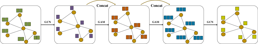
Figure 2. An illustration of our proposed GANet described in Section 3.3. In this example, the input graph contains 6 nodes, each of which has two features. A GCN layer is used to transform input feature vectors into low-dimensional representations. After that, we stack two GAMs for feature extraction. To facilitate feature reuse and gradients back-propagation, we add skip concatenation connections for GAMs. Finally, a GCN layer is used to output designated number of feature maps, which can be directly used for node classification predictions or used as inputs of following operations.

Both GAO and our hGAO use the node-wise attention mechanism in which the output feature vector of node $i$ is obtained by attending the input feature vector to all or selected neighboring nodes. Here, we propose to perform attention operation from the perspective of channels, resulting in our channel-wise graph attention operator (cGAO). For each channel $\boldsymbol{X}_{i:}$, we compute its responses by attending it to all channels. The layer-wise forward propagation function of cGAO can be expressed as

(11) $$\boldsymbol{E} =\boldsymbol{X}\boldsymbol{X}^{T} \in \mathbb{R}^{d\times d},$$

$$\boldsymbol{O} =\mbox{softmax}(\boldsymbol{E})\boldsymbol{X} \in \mathbb{R}^{d\times N}.$$

Note that we avoid the use of adjacency matrix $\boldsymbol{A}$, which is different from GAO and hGAO. When computing the coefficient matrix $\boldsymbol{E}$, the similarity score between two feature maps $\boldsymbol{X}_{i:}$ and $\boldsymbol{X}_{j:}$ are calculated by $e_{ij}=\sum_{k=1}^{N}X_{ik}\times X_{jk}$. It can be seen that features within the same node communicate with each other, and there is no communication among features located in different nodes. This means we do not need the connectivity information provided by adjacency matrix $\boldsymbol{A}$, thereby avoiding the dependency on the adjacency matrix used in node-wise attention operators. This saves computational resources related to operations with the adjacency matrix.

The computational cost of cGAO is $O(Nd^{2})$, which is lower than that of GAO if $d<N$. When applying attention operators on graph data, we can control the number of feature maps $d$, but it is hard to reduce the number of nodes in graphs. On large graphs with $d\ll N$, cGAO has computational advantages over GAO and hGAO, since its time complexity is only linear to the size of graphs. The space complexity of cGAO is $O(d^{2})$, which is independent of graph size. This means the application of cGAO on large graphs does not suffer from memory issues, which is especially useful on memory limited devices such as GPUs and mobile devices. Table 1 provides theoretical comparisons among GAO, hGAO and cGAO in terms of the time and space complexities. Therefore, cGAO enables efficient parallel training by removing the dependency on the adjacency matrix in graphs and significantly reduces the usage of computational resources.

Table 1. Comparison of time and space complexities among GAO, hGAO, and cGAO.

Operator	Time Complexity	Space Complexity
GAO	$O(N^{2}\times d)$	$O(N^{2})$
hGAO	$O(N\times\log N\times k+N\times k\times d^{2})$	$O(N^{2})$
cGAO	$O(N\times d^{2})$	$O(d^{2})$

3.3. The Proposed Graph Attention Networks

To use our hGAO and cGAO, we design a basic module known as the graph attention module (GAM). The GAM consists of two operators; those are, a graph attention operator and a graph convolutional network (GCN) layer (Kipf and Welling, 2017). We combine these two operators to enable efficient information propagation within graphs. For GAO and hGAO, they aggregate information from neighboring nodes by taking weighted sum of feature vectors from adjacent nodes. But there exists a situation that weights of some neighboring nodes are close to zero, preventing the information propagation of these nodes. In cGAO, the attention operator is applied among channels and does not involve information propagation among nodes. To overcome this limitation, we use a GCN layer, which applies the same weights to neighboring nodes and aggregate information from all adjacent nodes. Note that we can use any graph attention operator such as GAO, hGAO and cGAO. To facilitate feature reuse and gradients back-propagation, we add a skip connection by concatenating inputs and outputs of the GCN layer.

Based on GAM, we design graph attention networks, denoted as GANet, for network embedding learning. In GANet, we first apply a GCN layer, which acts as a graph embedding layer to produce low-dimensional representations for nodes. In some data like citation networks dataset (Kipf and Welling, 2017), nodes usually have very high-dimensional feature vectors. After the GCN layer, we stack multiple GAMs depending on the complexity of the graph data. As each GAM only aggregates information from neighboring nodes, stacking more GAMs can collect information from a larger parts of the graph. Finally, a GCN layer is used to produce designated number of output feature maps. The outputs can be directly used as predictions of node classification tasks. We can also add more operations to produce predictions for graph classification tasks. Figure 2 provides an example of our GANet. Based on this network architecture, we denote the networks using GAO, hGAO and cGAO as GANet, hGANet and cGANet, respectively.

Table 2. Statistics of datasets used in graph classification tasks under inductive learning settings. We use the D&D, PROTEINS, COLLAB, MUTAG, PTC, and IMDB-M datasets.

Dataset	Total Graphs	Train Graphs	Test Graphs	Nodes (max)	Nodes (avg)	Degree	Classes
MUTAG	188	170	18	28	17.93	2.19	2
PTC	344	310	34	109	25.56	1.99	2
PROTEINS	1113	1002	111	620	39.06	3.73	2
D&D	1178	1061	117	5748	284.32	4.98	2
IMDB-M	1500	1350	150	89	13.00	10.14	3
COLLAB	5000	4500	500	492	74.49	65.98	3

Table 3. Statistics of datasets used in node classification tasks under transductive learning settings. We use the Cora, Citeseer, and Pubmed datasets.

Dataset	Nodes	Features	Training	Validation	Testing	Degree	Classes
Cora	2708	1433	140	500	1000	4	7
Citeseer	3327	3703	120	500	1000	5	6
Pubmed	19717	500	60	500	1000	6	3

4. Experimental Studies

In this section, we evaluate our proposed graph attention networks on node classification and graph classification tasks. We first compare our hGAO and cGAO with GAO in terms of computation resources such as computational cost and memory usage. Next, we compare our hGANet and cGANet with prior state-of-the-art models under inductive and transductive learning settings. Performance studies among GAO, hGAO, and cGAO are conducted to show that our hGAO and cGAO achieve better performance than GAO. We also conduct some performance studies to investigate the selection of some hyper-parameters.

4.1. Datasets

We conduct experiments on graph classification tasks under inductive learning settings and node classification tasks under transductive learning settings. Under inductive learning settings, training and testing data are separate. The test data are not accessible during training time. The training process will not learn about graph structures of the test data. For graph classification tasks under inductive learning settings, we use the MUTAG (Niepert et al., 2016), PTC (Niepert et al., 2016), PROTEINS (Borgwardt et al., 2005), D&D (Dobson and Doig, 2003), IMDB-M (Yanardag and Vishwanathan, 2015), and COLLAB (Yanardag and Vishwanathan, 2015) datasets to fully evaluate our proposed methods. MUTAG, PTC, PROTEINS and D&D are four benchmarking bioinformatics datasets. MUTAG and PTC are much smaller than PROTEINS and D&D in terms of number of graphs and average nodes in graphs. Compared to large datasets, evaluations on small datasets can help investigate the risk of over-fitting, especially for deep learning based methods. COLLAB, IMDB-M are two social network datasets. For these datasets, we follow the same settings as in (Zhang et al., 2018), which employs 10-fold cross validation (Chang and Lin, 2011) with 9 folds for training and 1 fold for testing. The statistics of these datasets are summarized in Table 2.

Unlike inductive learning settings, the unlabeled data and graph structure are accessible during the training process under transductive learning settings. To be specific, only a small part of nodes in the graph are labeled while the others are not. For node classification tasks under transductive learning settings, we use three benchmarking datasets; those are Cora (Sen et al., 2008), Citeseer, and Pubmed (Kipf and Welling, 2017). These datasets are citation networks. Each node in the graph represents a document while an edge indicates a citation relationship. The graphs in these datasets are attributed and the feature vector of each node is generated by bag-of-word representations. The dimensions of feature vectors of three datasets are different depending on the sizes of dictionaries. Following the same experimental settings in (Kipf and Welling, 2017), we use 20 nodes, 500 nodes, and 500 nodes for training, validation, and testing, respectively.

Table 4. Comparison of results among GAO, hGAO, and cGAO on different graph sizes in terms of the number of MAdd, memory usage, and CPU prediction time. The input sizes are describe by “number of nodes $\times$ number of features”. The prediction time is the total execution time on CPU.

Input	Layer	MAdd	Cost Saving	Memory	Memory Saving	Time	Speedup
$1000\times 48$	GAO	100.61m	0.00%	4.98MB	0.00%	8.19ms	1.0$\times$
	hGAO	37.89m	62.34%	4.98MB	0.00%	5.61ms	1.46$\times$
	cGAO	9.21m	90.84%	0.99MB	80.12%	0.82ms	9.99$\times$
$10000\times 48$	GAO	9,646.08m	0.00%	409.6MB	0.00%	947.24ms	1.0$\times$
	hGAO	468.96m	95.14%	409.6MB	0.00%	371.12ms	2.55$\times$
	cGAO	92.16m	99.04%	9.61MB	97.65%	17.96ms	52.74$\times$
$20000\times 48$	GAO	38,492.16m	0.00%	1,619.2MB	0.00%	12,784.45ms	1.0$\times$
	hGAO	1,137.97m	97.04%	1,619.2MB	0.00%	4,548.62ms	2.81$\times$
	cGAO	184.32m	99.52%	19.2MB	98.81%	29.71ms	430.31$\times$

Table 5. Comparison of results of graph classification experiments with prior state-of-the-art models in terms of accuracies on the D&D, PROTEINS, COLLAB, MUTAG, PTC, and IMDB-M datasets. “-” denotes the result not available.

Models	D&D	PROTEINS	COLLAB	MUTAG	PTC	IMDB-M
GRAPHSAGE (Hamilton et al., 2017)	75.42%	70.48%	68.25%	-	-	-
PSCN (Niepert et al., 2016)	76.27%	75.00%	72.60%	88.95%	62.29%	45.23%
SET2SET (Vinyals et al., 2016)	78.12%	74.29%	71.75%	-	-	-
DGCNN (Zhang et al., 2018)	79.37%	76.26%	73.76%	85.83%	58.59%	47.83%
DiffPool (Ying et al., 2018)	80.64%	76.25%	75.48%	-	-	-
cGANet	80.86%	78.23%	76.96%	89.00%	63.53%	48.93%
hGANet	81.71%	78.65%	77.48%	90.00%	65.02%	49.06%

4.2. Experimental Setup

In this section, we describe the experimental setup for inductive learning and transductive learning tasks. For inductive learning tasks, we adopt the model architecture of DGCNN (Zhang et al., 2018). DGCNN consists of four parts; those are graph convolution layers, soft pooling, 1-D convolution layers and dense layers. We replace graph convolution layers with our hGANet described in Section 3.3 and the other parts remain the same. The hGANet contains a starting GCN layer, four GAMs and an ending GCN layer. Each GAM is composed of a hGAO, and a GCN layer. The starting GCN layer outputs 48 feature maps. Each hGAO and GCN layer within GAMs outputs 12 feature maps. The final GCN layer produces 97 feature maps as the original graph convolution layers in DGCNN. The skip connections using concatenation is employed between the input and output feature maps of each GAM. The hyper-parameter $k$ is set to 8 in each hGAO, which means each node in a graph selects 8 most important neighboring nodes to compute the response. We apply dropout (Srivastava et al., 2014) with the keep rate of 0.5 to the feature matrix in every GCN layer. For experiments on cGANet, we use the same settings.

For transductive learning tasks, we use our hGANet to perform node classification predictions. Since the feature vectors for nodes are generated using the bag-of-words method, they are high-dimensional sparse features. The first GCN layer acts like an embedding layer to reduce them into low-dimensional features. To be specific, the first GCN layer outputs 48 feature maps to produce 48 embedding features for each node. For different datasets, we stack different number of GAMs. Specifically, we use 4, 2, and 3 GAMs for Cora, Citeseer, and Pubmed, respectively. Each hGAO and GCN layer in GAMs outputs 16 feature maps. The last GCN layer produces the prediction on each node in the graph. We apply dropout with the keep rate of 0.12 on feature matrices in each layer. We also set $k$ to 8 in all hGAOs. We employ identity activation function as (Gao et al., 2018) for all layers in the model. To avoid over-fitting, we apply $L_{2}$ regularization with $\lambda=0.0001$. All trainable weights are initialized with Glorot initialization (Glorot and Bengio, 2010). We use Adam optimizer (Kingma and Ba, 2015) for training.

4.3. Comparison of Computational Efficiency

According to the theoretical analysis in Section 3, our proposed hGAO and cGAO have efficiency advantages over GAO in terms of the computational cost and memory usage. The advantages are expected to be more obvious as the increase of the number of nodes in a graph. In this section, we conduct simulated experiments to evaluate these theoretical analysis results. To reduce the influence of external factors, we use the network with a single graph attention operator and apply TensorFlow profile tool (Abadi et al., 2016) to report the number of multiply-adds (MAdd), memory usage, and CPU inference time on simulated graph data.

The simulated data are create with the shape of “number of nodes $\times$ number of feature maps”. For all simulated experiments, each node on the input graph has 48 features. We test three graph sizes; those are 1000, 1,0000, and 20,000, respectively. All tested graph operators output 48 feature maps including GAO, hGAO, and cGAO. For hGAOs, we set $k=8$ in all experiments, which is the value of hyper-parameter $k$ tuned on graph classification tasks. We report the number of MAdd, memory usage, and CPU inference time.

The comparison results are summarized in Table 4. On the graph with 20,000 nodes, our cGAO and hGAO provide 430.31 and 2.81 times speedup compared to GAO. In terms of the memory usage, cGAO can save 98.81% compared to GAO and hGAO. When comparing across different graph sizes, the effects of speedup and memory saving are more apparent as the graph size increases. This is consistent with our theoretical analysis on hGAO and cGAO. Our hGAO can save computational cost compared to GAO. cGAO achieves great computational resources reduction, which makes it applicable on large graphs. Note that the speed up of hGAO over GAO is not as apparent as the computational cost saving due to the practical implementation limitations.

Table 6. Comparison of results of node classification experiments with prior state-of-the-art models on the Cora, Citeseer, and Pubmed datasets.

Models	Cora	Citeseer	Pubmed
DeepWalk (Perozzi et al., 2014)	67.2%	43.2%	65.3%
Planetoid (Yang et al., 2016)	75.7%	64.7%	77.2%
Chebyshev (Defferrard et al., 2016)	81.2%	69.8%	74.4%
GCN (Kipf and Welling, 2017)	81.5%	70.3%	79.0%
GAT (Veličković et al., 2017)	83.0 $\pm$ 0.7%	72.5 $\pm$ 0.7%	79.0 $\pm$ 0.3%
hGANet	83.5 $\pm$ 0.7%	72.7 $\pm$ 0.6%	79.2 $\pm$ 0.4%

4.4. Results on Inductive Learning Tasks

Table 7. Comparison of results of graph classification experiments among GAO, hGAO, and cGAO in terms of accuracies on the D&D, PROTEINS, COLLAB, MUTAG, PTC, and IMDB-M datasets. “OOM” denotes out of memory.

Models	D&D	PROTEINS	COLLAB	MUTAG	PTC	IMDB-M
GANet	OOM	77.92%	76.06%	87.22%	62.94%	48.89%
cGANet	80.86%	78.23%	76.96%	89.00%	63.53%	48.93%
hGANet	81.71%	78.65%	77.48%	90.00%	65.02%	49.06%

We evaluate our methods on graph classification tasks under inductive learning settings. To compare our proposed cGAOs with hGAO and GAO, we replace hGAOs with cGAOs in hGANet, denoted as cGANet. We compare our models with prior sate-of-the-art models on D&D, PROTEINS, COLLAB, MUTAG, PTC, and IMDB-M datasets, which serve as the benchmarking datasets for graph classification tasks. The results are summarized in Table 5.

From the results, we can observe that the our hGANet consistently outperforms DiffPool (Ying et al., 2018) by margins of 0.90%, 1.40%, and 2.00% on D&D, PROTEINS, and COLLAB datasets, which contain relatively big graphs in terms of the average number of nodes in graphs. Compared to DGCNN, the performance advantages of our hGANet are even larger. The superior performances on large benchmarking datasets demonstrate that our proposed hGANet is promising since we only replace graph convolution layers in DGCNN. The performance boosts over the DGCNN are consistently and significant, which indicates the great capability on feature extraction of hGAO compared to GCN layers.

On datasets with smaller graphs, our GANets outperform prior state-of-the-art models by margins of 1.05%, 2.71%, and 1.23% on MUTAG, PTC, and IMDB-M datasets. The promising performances on small datasets prove that our methods improve the ability of high-level feature extraction without incurring the problem of over-fitting. cGANet outperforms prior state-of-the-art models but has lower performances than hGANet. This indicates that cGAO is also effective on feature extraction but not as powerful as hGAO. The attention on only important adjacent nodes incurred by using hGAOs helps to improve the performance on graph classification tasks.

4.5. Results on Transductive Learning Tasks

Under transductive learning settings, we evaluate our methods on node classification tasks. We compare our hGANet with prior state-of-the-art models on Cora, Citeseer, and Pubmed datasets in terms of the node classification accuracy. The results are summarized in Table 6. From the results, we can observe that our hGANet achieves consistently better performances than GAT, which is the prior state-of-the-art model using graph attention operator. Our hGANet outperforms GAT (Veličković et al., 2017) on three datasets by margins of 0.5%, 0.2%, and 0.2%, respectively. This demonstrates that our hGAO has performance advantage over GAO by attending less but most important adjacent nodes, leading to better generalization and performance.

4.6. Comparison of cGAO and hGAO with GAO

Besides comparisons with prior state-of-the-art models, we conduct experiments under inductive learning settings to compare our hGAO and cGAO with GAO. To be fair, we replace all hGAOs with GAOs in hGANet employed on graph classification tasks, which results in GANet. GAOs output the same number of feature maps as the corresponding hGAOs. Like hGAOs, we apply linear transformations on key and value matrices. This means GANets have nearly the same number of parameters with hGANets, which additionally contain limited number of projection vectors in hGAOs. We adopt the same experimental setups as hGANet. We compare our hGANet and cGANet with GANet on all six datasets for graph classification tasks described in Section 4.1. The comparison results are summarized in Table 7.

The results show that our cGAO and hGAO have significantly better performances than GAO. Notably, GANet runs out of memory when training on D&D dataset with the same experimental setup as hGANet. This demonstrates that hGAO has memory advantage over GAO in practice although they share the same space complexity. cGAO outperforms GAO on all six datasets but has slightly lower performances than hGAO. Considering cGAO dramatically saves computational resources, cGAO is a good choice when facing large graphs. Since there is no work that realizes the hard attention operator in (Xu et al., 2015) on graph data, we do not provide comparisons with it in this work.

4.7. Performance Study of $k$ in hGAO

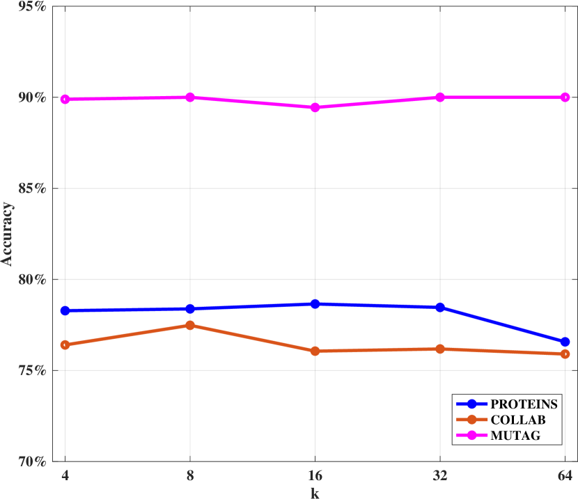
Figure 3. Results of employing different $k$ values in hGAOs using hGANet on PROTEINS, COLLAB, and MUTAG datasets under inductive learning settings. We use the same experimental setups described in Section 4.2. We report the graph classification accuracies in this figure. We can see that the best performances is achieved when $k=8$.

Since $k$ is an important hyper-parameter in hGAO, we conduct experiments to investigate the impact of different $k$ values on hGANet. Based on hGANet, we vary the values of $k$ in hGAOs with choices of 4, 8, 16, 32, and 64, which are reasonable selections for $k$. We report performances of hGANets with different $k$ values on graph classification tasks on PROTEINS, COLLAB, and MUTAG datasets, which cover both large and small datasets.

The performance changes of hGANets with different $k$ values are plotted in Figure 3. From the figure, we can see that hGANets achieve the best performances on all three datasets when $k=8$. The performances start to decrease as the increase of $k$ values. On PROTEINS and COLLAB datasets, the performances of hGANets with $k=64$ are significantly lower than those with $k=8$. This indicates that larger $k$ values make the query node to attend more adjacent nodes in hGAO, which leads to worse generalization and performance.

5. Conclusions

In this work, we propose novel hGAO and cGAO which are attention operators on graph data. hGAO achieves the hard attention operation by selecting important nodes for the query node to attend. By employing a trainable projection vector, hGAO selects $k$-most important nodes for each query node based on their projection scores. Compared to GAO, hGAO saves computational resources and attends important adjacent nodes, leading to better generalization and performance. Furthermore, we propose the cGAO, which performs attention operators from the perspective of channels. cGAO removes the dependency on the adjacency matrix and dramatically saves computational resources compared to GAO and hGAO. Based on our proposed attention operators, we propose a new architecture that employs a densely connected design pattern to promote feature reuse. We evaluate our methods under both transductive and inductive learning settings. Experimental results demonstrate that our hGANets achieve improved performance compared to prior state-of-the-art networks. The comparison between our methods and GAO indicates that our hGAO achieves significant better performance than GAO. Our cGAO greatly saves computational resources and makes attention operators applicable on large graphs.

- (1)
- Abadi et al. (2016) Martín Abadi, Paul Barham, Jianmin Chen, Zhifeng Chen, Andy Davis, Jeffrey Dean, Matthieu Devin, Sanjay Ghemawat, Geoffrey Irving, Michael Isard, et al. 2016. Tensorflow: a system for large-scale machine learning. In OSDI, Vol. 16. 265–283.
- Borgwardt et al. (2005) Karsten M Borgwardt, Cheng Soon Ong, Stefan Schönauer, SVN Vishwanathan, Alex J Smola, and Hans-Peter Kriegel. 2005. Protein function prediction via graph kernels. Bioinformatics 21, suppl_1 (2005), i47–i56.
- Chang and Lin (2011) Chih-Chung Chang and Chih-Jen Lin. 2011. LIBSVM: a library for support vector machines. ACM Transactions on Intelligent Systems and Technology 2, 3 (2011), 27.
- Defferrard et al. (2016) Michaël Defferrard, Xavier Bresson, and Pierre Vandergheynst. 2016. Convolutional neural networks on graphs with fast localized spectral filtering. In Advances in Neural Information Processing Systems. 3844–3852.
- Devlin et al. (2018) Jacob Devlin, Ming-Wei Chang, Kenton Lee, and Kristina Toutanova. 2018. Bert: Pre-training of deep bidirectional transformers for language understanding. arXiv preprint arXiv:1810.04805 (2018).
- Dobson and Doig (2003) Paul D Dobson and Andrew J Doig. 2003. Distinguishing enzyme structures from non-enzymes without alignments. Journal of Molecular Biology 330, 4 (2003), 771–783.
- Gao et al. (2018) Hongyang Gao, Zhengyang Wang, and Shuiwang Ji. 2018. Large-scale learnable graph convolutional networks. In Proceedings of the 24th ACM SIGKDD International Conference on Knowledge Discovery & Data Mining. ACM, 1416–1424.
- Glorot and Bengio (2010) Xavier Glorot and Yoshua Bengio. 2010. Understanding the difficulty of training deep feedforward neural networks. In Proceedings of the Thirteenth International Conference on Artificial Intelligence and Statistics. 249–256.
- Gregor et al. (2015) Karol Gregor, Ivo Danihelka, Alex Graves, Danilo Rezende, and Daan Wierstra. 2015. DRAW: A recurrent neural network for image generation. In International Conference on Machine Learning. 1462–1471.
- Hamilton et al. (2017) Will Hamilton, Zhitao Ying, and Jure Leskovec. 2017. Inductive representation learning on large graphs. In Advances in Neural Information Processing Systems. 1024–1034.
- Hochreiter and Schmidhuber (1997) Sepp Hochreiter and Jürgen Schmidhuber. 1997. Long short-term memory. Neural Computation 9, 8 (1997), 1735–1780.
- Jaderberg et al. (2015) Max Jaderberg, Karen Simonyan, Andrew Zisserman, et al. 2015. Spatial transformer networks. In Advances in Neural Information Processing Systems. 2017–2025.
- Juefei-Xu et al. (2016) Felix Juefei-Xu, Eshan Verma, Parag Goel, Anisha Cherodian, and Marios Savvides. 2016. Deepgender: Occlusion and low resolution robust facial gender classification via progressively trained convolutional neural networks with attention. In Proceedings of the IEEE Conference on Computer Vision and Pattern Recognition Workshops. 68–77.
- Kingma and Ba (2015) Diederik Kingma and Jimmy Ba. 2015. Adam: A method for stochastic optimization. The International Conference on Learning Representations (2015).
- Kipf and Welling (2017) Thomas N Kipf and Max Welling. 2017. Semi-supervised classification with graph convolutional networks. International Conference on Learning Representations (2017).
- LeCun et al. (2012) Yann LeCun, Léon Bottou, Genevieve B Orr, and Klaus-Robert Müller. 2012. Efficient backprop. In Neural networks: Tricks of the trade. Springer, 9–48.
- Li et al. (2018) Guanbin Li, Xiang He, Wei Zhang, Huiyou Chang, Le Dong, and Liang Lin. 2018. Non-locally enhanced encoder-decoder network for single image de-raining. In 2018 ACM Multimedia Conference on Multimedia Conference. ACM, 1056–1064.
- Ling and Rush (2017) Jeffrey Ling and Alexander Rush. 2017. Coarse-to-fine attention models for document summarization. In Proceedings of the Workshop on New Frontiers in Summarization. 33–42.
- Luong et al. (2015) Thang Luong, Hieu Pham, and Christopher D Manning. 2015. Effective approaches to attention-based neural machine translation. In Proceedings of the 2015 Conference on Empirical Methods in Natural Language Processing. 1412–1421.
- Malinowski et al. (2018) Mateusz Malinowski, Carl Doersch, Adam Santoro, and Peter Battaglia. 2018. Learning visual question answering by bootstrapping hard attention. In European Conference on Computer Vision. Springer, 3–20.
- Niepert et al. (2016) Mathias Niepert, Mohamed Ahmed, and Konstantin Kutzkov. 2016. Learning convolutional neural networks for graphs. In International Conference on Machine Learning. 2014–2023.
- Perozzi et al. (2014) Bryan Perozzi, Rami Al-Rfou, and Steven Skiena. 2014. Deepwalk: Online learning of social representations. In Proceedings of the 20th ACM SIGKDD International Conference on Knowledge Discovery and Data Mining. 701–710.
- Rao et al. (2017) Yongming Rao, Jiwen Lu, and Jie Zhou. 2017. Attention-aware deep reinforcement learning for video face recognition. In Proceedings of the IEEE Conference on Computer Vision and Pattern Recognition. 3931–3940.
- Sen et al. (2008) Prithviraj Sen, Galileo Namata, Mustafa Bilgic, Lise Getoor, Brian Galligher, and Tina Eliassi-Rad. 2008. Collective classification in network data. AI Magazine 29, 3 (2008), 93.
- Shankar et al. (2018) Shiv Shankar, Siddhant Garg, and Sunita Sarawagi. 2018. Surprisingly easy hard-attention for sequence to sequence learning. In Proceedings of the 2018 Conference on Empirical Methods in Natural Language Processing. 640–645.
- Srivastava et al. (2014) Nitish Srivastava, Geoffrey Hinton, Alex Krizhevsky, Ilya Sutskever, and Ruslan Salakhutdinov. 2014. Dropout: A simple way to prevent neural networks from overfitting. Journal of Machine Learning Research 15, 1 (2014), 1929–1958.
- Vaswani et al. (2017) Ashish Vaswani, Noam Shazeer, Niki Parmar, Jakob Uszkoreit, Llion Jones, Aidan N Gomez, Łukasz Kaiser, and Illia Polosukhin. 2017. Attention is all you need. In Advances in Neural Information Processing Systems. 6000–6010.
- Veličković et al. (2017) Petar Veličković, Guillem Cucurull, Arantxa Casanova, Adriana Romero, Pietro Liò, and Yoshua Bengio. 2017. Graph attention networks. In International Conference on Learning Representations.
- Vinyals et al. (2016) Oriol Vinyals, Samy Bengio, and Manjunath Kudlur. 2016. Order matters: Sequence to sequence for sets. International Conference on Learning Representations (2016).
- Wang et al. (2018) Xiaolong Wang, Ross Girshick, Abhinav Gupta, and Kaiming He. 2018. Non-local neural networks. In The IEEE Conference on Computer Vision and Pattern Recognition, Vol. 1. 4.
- Xu et al. (2015) Kelvin Xu, Jimmy Ba, Ryan Kiros, Kyunghyun Cho, Aaron Courville, Ruslan Salakhudinov, Rich Zemel, and Yoshua Bengio. 2015. Show, attend and tell: Neural image caption generation with visual attention. In International Conference on Machine Learning. 2048–2057.
- Yanardag and Vishwanathan (2015) Pinar Yanardag and SVN Vishwanathan. 2015. A structural smoothing framework for robust graph comparison. In Advances in Neural Information Processing Systems. 2134–2142.
- Yang et al. (2016) Zhilin Yang, William Cohen, and Ruslan Salakhudinov. 2016. Revisiting semi-supervised learning with graph embeddings. In International Conference on Machine Learning. 40–48.
- Ying et al. (2018) Zhitao Ying, Jiaxuan You, Christopher Morris, Xiang Ren, Will Hamilton, and Jure Leskovec. 2018. Hierarchical graph representation learning with differentiable pooling. In Advances in Neural Information Processing Systems. 4800–4810.
- Yu et al. (2019) Bing Yu, Haoteng Yin, and Zhanxing Zhu. 2019. ST-UNet: A spatio-temporal U-network for graph-structured time series modeling. arXiv preprint arXiv:1903.05631 (2019).
- Zhang et al. (2018) Muhan Zhang, Zhicheng Cui, Marion Neumann, and Yixin Chen. 2018. An end-to-end deep learning architecture for graph classification. In Proceedings of AAAI Conference on Artificial Inteligence.
- Zhao et al. (2018) Hengshuang Zhao, Yi Zhang, Shu Liu, Jianping Shi, Chen Change Loy, Dahua Lin, and Jiaya Jia. 2018. Psanet: Point-wise spatial attention network for scene parsing. In Proceedings of the European Conference on Computer Vision. 267–283.