Comparison of the optical light curves of hydrogen-rich and hydrogen-poor type II supernovae

Abstract

Type II supernovae (SNe II) show strong hydrogen features in their spectra throughout their whole evolution while type IIb supernovae (SNe IIb) spectra evolve from dominant hydrogen lines at early times to increasingly strong helium features later on. However, it is currently unclear whether the progenitors of these supernova (SN) types form a continuum in pre-SN hydrogen mass or whether they are physically distinct. SN light-curve morphology directly relates to progenitor and explosion properties such as the amount of hydrogen in the envelope, the pre-SN radius, the explosion energy and the synthesized mass of radioactive material. In this work we study the morphology of the optical-wavelength light curves of hydrogen-rich SNe II and hydrogen-poor SNe IIb to test whether an observational continuum exists between the two. Using a sample of 95 SNe (73 SNe II and 22 SNe IIb), we define a range of key observational parameters and present a comparative analysis between both types. We find a lack of events that bridge the observed properties of SNe II and SNe IIb. Light curve parameters such as rise times and post-maximum decline rates and curvatures clearly separate both SN types and we therefore conclude that there is no continuum, with the two SN types forming two observationally distinct families. In the $V$-band a rise time of 17 days (SNe II lower, SNe IIb higher), and a magnitude difference between 30 and 40 days post explosion of 0.4 mag (SNe II lower, SNe IIb higher) serve as approximate thresholds to differentiate both types.

1 Introduction

It is believed that stars with initial masses $>$ 8${\rm\ M}_{\odot}$  end their lives exploding as core collapse SNe (CCSNe). CCSNe can be divided into two main groups based on their spectral properties. Those SNe that show hydrogen in their spectra are classified as Type II supernovae (SNe II) while those that do not are of Type I (Minkowski 1941, see Gal-Yam 2017 and references therein for a review of spectroscopic SNe classification). Subsequent division of SNe II into “plateau” (IIP) and “linear” (IIL) was introduced based on the shape of the light curve (Barbon et al. 1979), however recent works have found a continuum of observed properties between the two (Anderson et al. 2014, Sanders et al. 2015, Galbany et al. 2016, Rubin & Gal-Yam 2016). Therefore, we refer to these two historical groups together as “hydrogen-rich SNe II” for the remainder of this work. A number of further sub-classifications exists, such as those SNe II showing similar properties to SN 1987A (with particularly long-rising light curves, see e.g. Pastorello et al. 2012, Taddia et al. 2016 and references therein), and those displaying narrow emission features in their spectra, the Type IIn (Schlegel 1990). However, both of these groups show characteristics sufficiently distinct from hydrogen-rich SNe II (as defined above) that we do not consider them in this work (see Arcavi 2017 and references therein for additional discussion on hydrogen-rich CCSNe). Type I CCSNe were also separated into Types Ib and Ic based on the presence or absence of helium lines in their spectra (see Filippenko 1997, Gal-Yam 2017 and references therein). Due to the lack of hydrogen these latter events are also referred to as stripped-envelope SNe (SE SNe) in reference to their progenitors having lost most, if not all, of their hydrogen envelopes before explosion. SNe Ib and SNe Ic are not studied in the present work.

An intermediate group named Type IIb was identified that undergoes a transition from a hydrogen-rich (similar to SNe II) to a hydrogen-poor (similar to SNe Ib) spectrum (Filippenko et al. 1993). This transition is attributed to a small amount of hydrogen in their progenitor envelopes, and we thus refer to this group simply as “SNe IIb” here. Their characteristic bell-shaped light curve, in addition to their overall similarity to SNe Ib and SNe Ic, has led the community to associate SNe IIb with SE SNe (e.g., Clocchiatti et al. 1996, Matheson et al. 2001) and model the main peak of SN IIb light curves as powered by radioactive decay of ⁵⁶Ni (e.g. Shigeyama et al. 1994, Woosley et al. 1994, Bersten et al. 2012). However, there are few studies that focus on a quantitative comparison of light-curve morphologies between SNe II and SNe IIb (c.f.: Arcavi et al. 2012, Faran et al. 2014, Eldridge et al. 2018).

An outstanding question in the study of CCSNe observations and their implications for our understanding of progenitor systems, is whether in spite of the spectroscopic distinction at late times, the early spectral similarities of SNe II and SNe IIb imply a shared common origin. Theoretical works have suggested that the majority (if not all) SNe IIb could come from interacting binaries (see e.g. Podsiadlowski et al. 1992, Nomoto et al. 1995, Benvenuto et al. 2013, Yoon et al. 2017, Gilkis et al. 2019). Although the bulk of hydrogen-rich SNe can be satisfactorily explained by the single-progenitor scenario, in principle some SNe II may also come from binary systems. For isolated stars the degree of envelope stripping should be chiefly dictated by the initial progenitor mass (with some additional dependence on progenitor metallicity, see e.g. Heger et al. 2003a). However, the situation is complicated by the effect of mass transfer in binary progenitors. Investigating whether SNe II and SNe IIb arise from similar or distinct progenitor scenarios can shed light on the importance of these competing mass-loss mechanisms.

It has been argued that the diversity in the light curves of hydrogen-rich SNe II is driven by the mass of the hydrogen envelope retained by the progenitor at the epoch of explosion. This follows early theoretical modelling of SNe II (Popov 1993) claiming that faster declining SNe II (that also show shorter-duration plateau phases, see e.g. Litvinova & Nadezhin 1983, Young 2004 for theoretical evidence and Anderson et al. 2014, Gutiérrez et al. 2017b for observational evidence of this phenomenon) arise from progenitors with lower mass envelopes. Since the hydrogen lines of SN IIb spectra disappear with time, it is believed that their progenitors retain an even smaller fraction of their hydrogen. If there were indeed a continuum of hydrogen envelope mass between the progenitors of SNe II and SNe IIb then we may expect to see a continuum in their observable light curve properties, similar to what is seen between fast and slow declining hydrogen-rich SNe II.

Arcavi et al. (2012) studied the light curve behaviour of a sample of 15 SNe IIb and SNe II in the $R$-band and argued that they separate into three distinct groups according to light curve shape: IIP, IIL, and IIb. Faran et al. (2014) studied 11 fast-declining SNe II (IIL) and found that they seem to be photometrically related to SNe IIb. Here, our study follows those previous works, using a larger sample and the addition of a range of observational parameters defined consistently across all SN types. We present an analysis of 95 SNe (73 hydrogen-rich SNe II and 22 SNe IIb) with the aim of determining whether there is a clear distinction in the shape of the light curves between these SNe subtypes, or whether a continuum is observed.

The paper is organized as follows: in Section 2 we present the data sample. In Section 3 we describe our light curve analysis method and explain how we obtain explosion and maximum-light epochs. Section 4 introduces the parameters we have used to compare light curve properties. Results are provided in Section 5. Section 6 presents a discussion of deviating cases and possible implications for progenitor properties. Finally in Section 7 we present our conclusions. In addition, an appendix is included where figures not included in the main body of the manuscript are presented along with tables containing information on each SN considered and the numeric values of the defined comparison parameters.

2 Supernova samples

Our sample includes 73 SNe II (see Table 5), with 64 taken from the Carnegie Type II Supernova Program (CATS; Galbany et al. 2016; PI: Hamuy, 2002$-$2003) and the Carnegie Supernova Project (CSP-I; Hamuy et al. 2006; PIs: Phillips and Hamuy, 2004$-$2009) samples from the work of Anderson et al. (2014). This sample was selected as it originated from a well defined dataset that was observed, reduced and calibrated in a consistent manner. Additionally, nine objects having well-defined light curve maxima were included from the literature. All the objects with well defined light curve maxima were then used as templates to obtain the date of maximum light for the rest of the sample. This was required because such dates were generally poorly constrained in Anderson et al. (2014), but are necessary to obtain rise times (see Sec. 5.1): an important parameter differentiating SNe II from SNe IIb. In the case of SNe IIb, no sufficiently large sample exists from a single follow-up program. Therefore, we collate all SNe IIb from the literature (see Table 7) that fit the following selection criteria (that also apply to the SNe II):

• Good sampling. At least nine data points in our primary photometric band ($V$), in order to have a good approximation of the intrinsic shape of the light curve.

• Existing photometric data points around maximum light for SNe IIb and prior to $\sim$25 days after explosion for SNe II to have a dense enough coverage of the early part of the light curve. This means that our SN II light curves do not necessarily cover the epoch of maximum light.

• When the explosion date is not well constrained by prediscovery non-detections, at least three available spectra in order to be able to estimate the explosion dates through spectral matching (see Section 3.1).

The parameters defined in this work (see Section 4) are only constrained by photometric data points up to $\sim$60 days after explosion. The reasons to adopt this limit are: a) to enable a characterization of the light curve properties around maximum light and the subsequent initial decline; and b) the light-curve coverage is more uniform among the SN sample than at later times. We choose $V$ as our primary photometric band as historically this is the band in which most SNe were observed with the best cadence. $B$- and $r$-band were also considered in order to study how the light curves behave at shorter and longer wavelengths, respectively. K-corrections have not been performed to the SN photometry. However, given the redshift range considered here (z < 0.08), such corrections are too small to affect our analysis. Also, all time intervals are given in the SN rest frame.

3 Light curves

To be able to compare the light curves and define the parameters described in Section 4 in a consistent manner, a uniform sampling of the light curve is needed. Hence, we resample the photometry via the Gaussian process method (see Rasmussen & Williams 2006 for details on Gaussian processes) using a self-made code that implements the Python library GPy (2012), using a squared-exponential kernel plus a kernel to account for the errors in the measured magnitudes. After running the code we not only obtain a regular sampling but also an uncertainty or confidence interval of said sampling. An example of the Gaussian process fit is presented in Fig. 1.

The Gaussian process works well when the photometry is well sampled. However, when the data points are not evenly sampled, the method tends to introduce spurious wiggles. At the same time, the confidence interval increases to accommodate to the lack of data. In our sample this effect is only considerable for the late part of the light curve, which is not considered in the analysis.

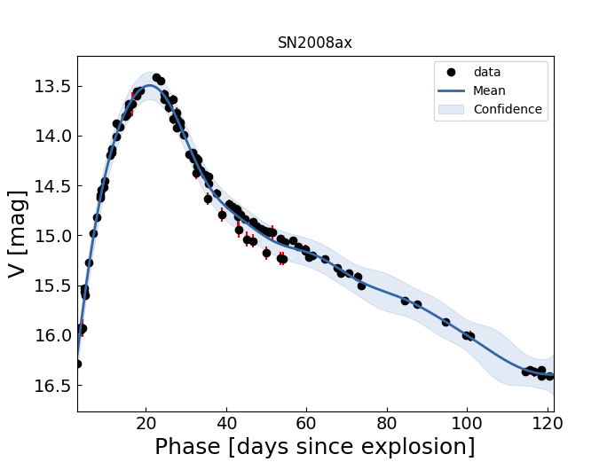
Figure 1: Resampled light curve of SN 2008ax. The black dots are the original photometric data points (obtained from different sources, see Table 7, hence the observable offset). Some error bars are smaller than the dot size. The mean of the resampling is presented as a blue continuous line and the confidence interval is presented in light blue.

3.1 Explosion epoch estimation

CSP-I and CATS SN II dates of explosion are those published in Gutiérrez et al. (2017a), which are a combination of explosion epochs from spectral matching and prediscovery non-detections. For the SNe II from other sources, we derive explosion epochs in the same way as Gutiérrez et al. (2017a). Whenever the interval between the last non-detection and the first detection is shorter than 20 days, the mid point of the interval is adopted as the explosion date and its uncertainty is set as half the interval length. When the previous requirement is not met, we use the spectral matching tool SNID (Supernova Identification software, Blondin & Tonry 2007) to derive an explosion date. In order to do this, we have added the spectra from Gutiérrez et al. (2017a) as SNID templates.

In the case of SNe IIb we create additional SNID templates using those events where the explosion epoch is well constrained from the discovery data (i.e., an interval shorter than 20 days between last non-detection and discovery). For the rest of the SNe IIb (without constraining non detections) we run SNID on each of their spectra. From each SNID run we select the spectral matches that provide an estimated age from maximum light that is within five days from the known age based on the light-curve fit. Every spectral match provides an age from explosion ($t_{\mathrm{exp\_match}}$) for the given spectrum. These $t_{\mathrm{exp\_match}}$ have an associated uncertainty that is given by that of the date of explosion of the SN template. We fix a minimum uncertainty of five days to account for the typical uncertainty in the spectral matching procedure, that is mainly determined by the size and diversity of the available template sample. Using the observation epoch ($t_{\mathrm{obs}}$) of the fitted spectrum we can compute a date of explosion for each match as $t_{\mathrm{obs}}-t_{\mathrm{exp\_match}}$. Finally, we compute the explosion date for the given SN IIb as the weighted average of the results from all selected SNID matches.

To test the validity of this procedure we remove each SN IIb template from the SNID library and calculate its explosion epoch as above. The results are presented in Table 1. The average difference between the explosion epoch calculated with SNID and the one calculated from non-detections is of $-0.65\pm 5.0$ days, which validates our procedure.

Table 1: Comparison between the explosion epochs obtained from non-detection constraints and those calculated using SNID for SNe IIb.

SNID		Observed
SN	Exp[MJD]	e_Exp	Exp[MJD]	e_Exp	diff
1993J	49074.4	5.79	49071.7	2.60	2.7
2004ex	53286.9	7.68	53288.8	0.50	-1.9
2004ff	53291.4	3.25	53302.9	3.49	-11.5
2006el	53964.0	7.88	53968.8	3.48	-4.8
2006T	53760.5	7.69	53759.0	7.02	1.5
2008aq	54508.0	9.51	54514.9	8.48	-6.9
2008ax	54529.4	6.85	54528.3	0.13	1.1
2009K	54850.2	9.12	54843.6	1.49	6.6
2011dh	55712.1	8.19	55712.4	0.52	-0.3
2013df	56448.2	5.04	56443.9	6.93	4.3
2016gkg	57653.2	10.07	57651.2	0.06	2.0

3.2 Maximum light epoch estimation

In the case of SNe IIb, we consider only the main maximum (thought to be powered by radioactive decay), and not that which occurs earlier during the cooling phase (see e.g. Bersten et al. 2012). The date of the main maximum is taken from the light curve through the Gaussian process resampling. To determine an error on the epoch of maximum light we adopted the mean separation in time between subsequent data points in the range from 15 days before to 15 days after maximum. This takes into account the uncertainty introduced by the cadence of the observations.

In the case of hydrogen-rich SNe II, when possible, the date of maximum is obtained directly from the resampled light curve, in the same way as described for SNe IIb. However, most of the objects in the sample of Anderson et al. (2014) do not have a well-observed maximum. In order to estimate the light curve maxima for those objects we searched the literature for SNe II where the epoch of maximum light was observed. The spectra of these SNe were then used to produce additional SNID templates. SNID was then run for the rest of the sample. If the difference between the age of explosion of the sample spectrum (calculated in the previous section) and the age of explosion of the template is less than five days, the template is considered a good match and it is used to estimate the epoch of maximum light. Again we cross-validate this procedure by removing each SN II used as a template, running that template through our steps, and comparing the values estimated using SNID with those obtained directly from the re-sampled light curve. To further test this method, the same was done with SNe IIb. The results are presented in Table 2. Average differences on the maximum light for SNe II is $-0.93\pm 4.6$ days, again validating our procedure.

Table 2: Comparison between the date of maximum light in the $V$-band obtained directly from SN photometry and that obtained from SNID for SNe II (top) and SNe IIb (bottom).

SNID		Observed
SNII	Max[MJD]	e_Max	Max[MJD]	e_Max	diff
1999gi	51529.0	3.76	51529.2	2.20	-0.2
2002gd	52564.5	4.84	52562.6	2.31	1.9
2004er	53284.7	5.23	53287.6	1.78	-2.9
2007U	54146.1	3.97	54144.9	3.32	1.2
2009ib	55054.4	4.52	55057.1	1.63	-2.7
2012aw	56015.7	4.72	56012.5	0.61	3.2
2013ai	56352.4	3.39	56365.4	1.00	-13.0
2013by	56413.7	4.37	56414.7	1.10	-1.0
2013ej	56509.2	4.58	56510.4	0.91	-1.2
2013fs	56584.3	4.46	56578.1	2.01	6.2
2014cx	56914.5	2.88	56917.5	0.77	-3.0
2014G	56682.0	4.34	56681.7	0.61	0.3
SNIIb	Max[MJD]	e_Max	Max[MJD]	e_Max	diff
1993J	49093.6	3.6	49095.0	0.11	1.4
1996cb	50450.6	3.1	50450.4	1.84	0.2
2003bg	52718.8	3.3	52717.6	10.3	1.2
2004ex	53311.3	3.0	53307.2	1.81	4.1
2004ff	53323.3	3.0	53313.1	1.88	10.2
2005Q	53408.1	4.0	53406.4	1.50	1.7
2006ba	53825.5	3.2	53823.1	2.49	2.4
2006el	53983.9	3.2	53983.8	1.60	0.1
2006T	53780.5	4.2	53780.3	1.74	0.2
2008aq	54537.0	3.3	54532.0	1.35	5.7
2008ax	54548.3	5.1	54549.6	0.52	-1.3
2008bo	54569.0	3.1	54567.6	1.21	1.4
2009mg	55190.6	3.3	55188.5	2.04	2.1
2009K	54864.5	4.7	54869.4	2.37	-4.9
2009Z	54881.4	2.7	54877.7	2.37	3.7
2010jr	-	-	55531.7	1.60	-
2011dh	55733.3	6.5	55732.1	0.88	1.2
2011ei	55785.1	3.0	55784.4	0.91	0.7
2011fu	55847.0	4.5	55846.0	0.49	1.0
2011hs	55889.8	3.5	55888.2	0.75	1.6
2013ak	56370.4	3.6	56368.8	1.79	1.6
2013df	56466.3	3.2	56469.8	0.38	-3.5
2016gkg	57671.9	4.3	57671.7	1.92	0.2

Both SNe II and SNe IIb have fewer objects with well-sampled light curve peaks in the $B$- and $r$-band. For those that do have a well-sampled peak, the maximum date is obtained directly from the photometry. For these same SNe we then calculate the weighted average of the difference of JD at peak for $V$ and $B$ together with $V$ and $r$, using as weights the errors on the determination of the date of maximum light. Results are presented in Table 3. These average differences are then used to estimate the date of maximum in $B$ and $r$ for the rest of the objects as the difference between the SN maximum epoch in $V$ and the weighted average of the corresponding band.

Table 3: Weighted average and error of $B_{\mathrm{max}}\,-\,V_{\mathrm{max}}$ and $V_{\mathrm{max}}\,-\,r_{\mathrm{max}}$, considering only those SNe with data points before light curve peak.

Type	$\#$SNe	Band	Weighted average	error
IIb	20	$B_{\mathrm{max}}\,-\,V_{\mathrm{max}}$	-1.32	0.40
	10	$V_{\mathrm{max}}\,-\,r_{\mathrm{max}}$	-0.56	0.75
II	8	$B_{\mathrm{max}}\,-\,V_{\mathrm{max}}$	-5.03	2.14
	8	$V_{\mathrm{max}}\,-\,r_{\mathrm{max}}$	-3.04	2.66

4 Resampled SN light curves and observational parameters

In this section we first present the resampled $V$-band hydrogen-rich SN II and SN IIb light curves and discuss their morphology. A number of observational parameters are then defined. These are used to compare the two SN types quantitatively in Section 5.

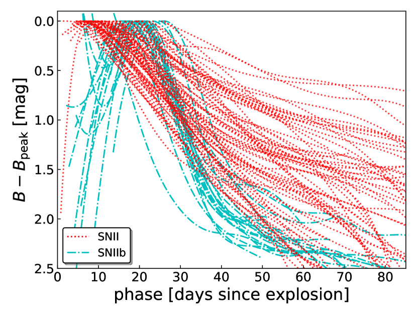
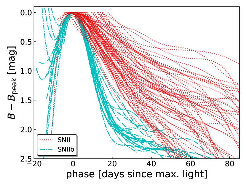
Figure 10: Resampled light curves normalized with respect to the $B$-band peak magnitude, SNe II are plotted in red dotted lines while SNe IIb are plotted in cyan dash-dot lines. Top panel: phase with respect to explosion epoch. Bottom panel: phase with respect to date of maximum light.

In Fig. 2 we present the resampled light curves normalized to the peak magnitude in $V$-band (if peak magnitude is not observed, the magnitude of the first photometric data point is used), both with respect to explosion date and to epoch of maximum light. Similar plots can be seen for $B$ and $r$ bands in Fig. 10 and Fig. 11 respectively.

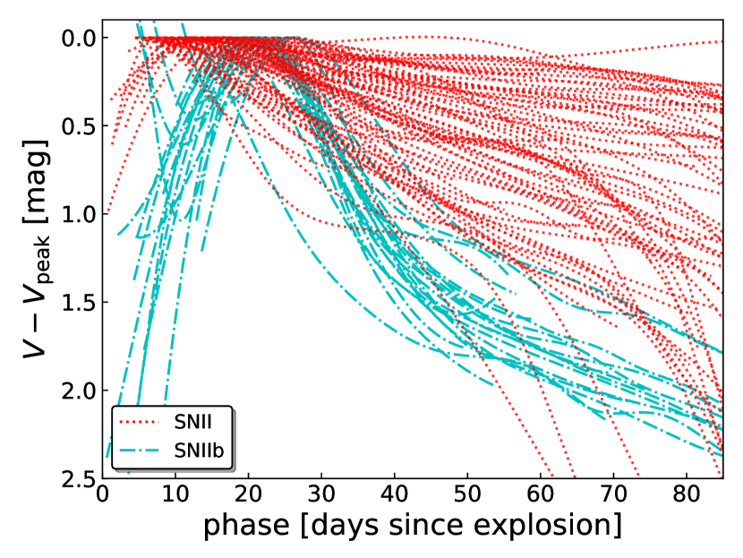
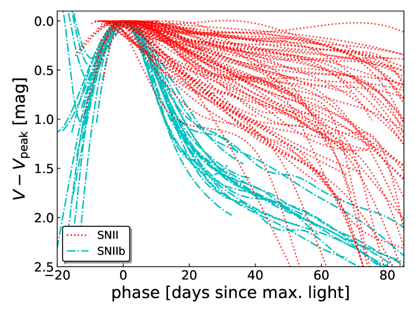
Figure 2: Resampled light curves normalized with respect to the $V$-band peak magnitude. SNe II are plotted in red dotted lines while SNe IIb are plotted in cyan dash-dot lines. Top panel: phase with respect to explosion epoch. Bottom panel: phase with respect to date of maximum light. Similar plots are presented for $B$- and $r$-band in the Appendix A.

The different behaviour of SNe II and SNe IIb can be seen in a qualitative, visual manner in these figures: SNe IIb take a longer time to reach maximum light (see top panel of Fig. 2) and decline more quickly post maximum (most easily seen in the bottom panel of Fig. 2) than SNe II. SNe IIb show a change in curvature following the first decline after peak, commonly thought to be the radioactive decay tail. This behaviour is not observed in SNe II; even though some of them show a change in the curvature, they generally seem to have a small “plateau” before continuing to decline.

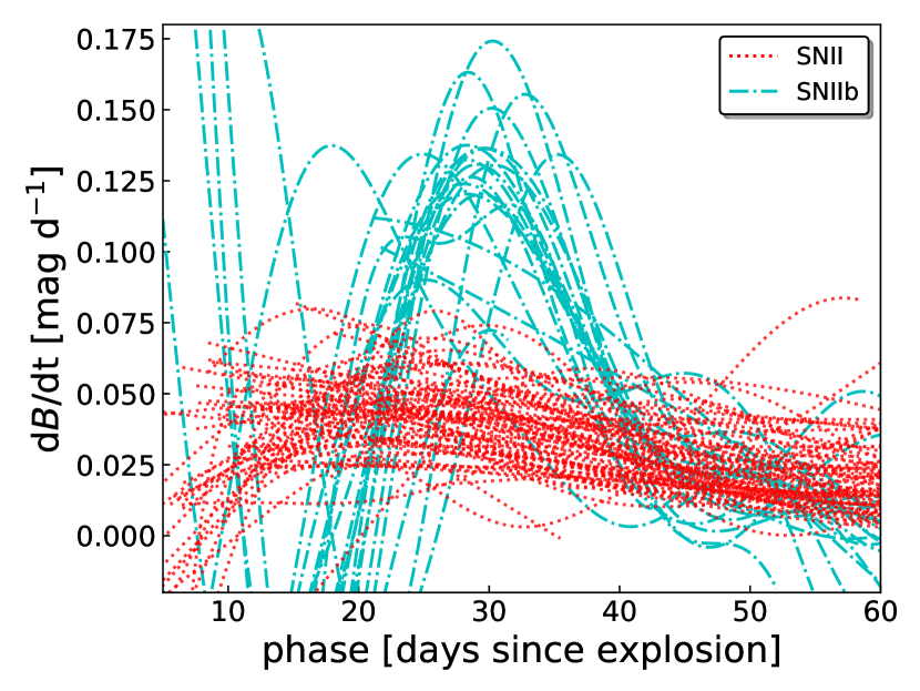
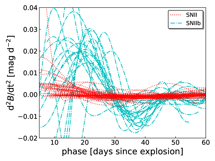
Figure 12: Derivative of the $B$-band light curve with respect to explosion. SNe II are plotted in red dotted lines while SNe IIb are plotted in cyan dash-dot lines. Top panel: first derivative. Bottom panel: second derivative.

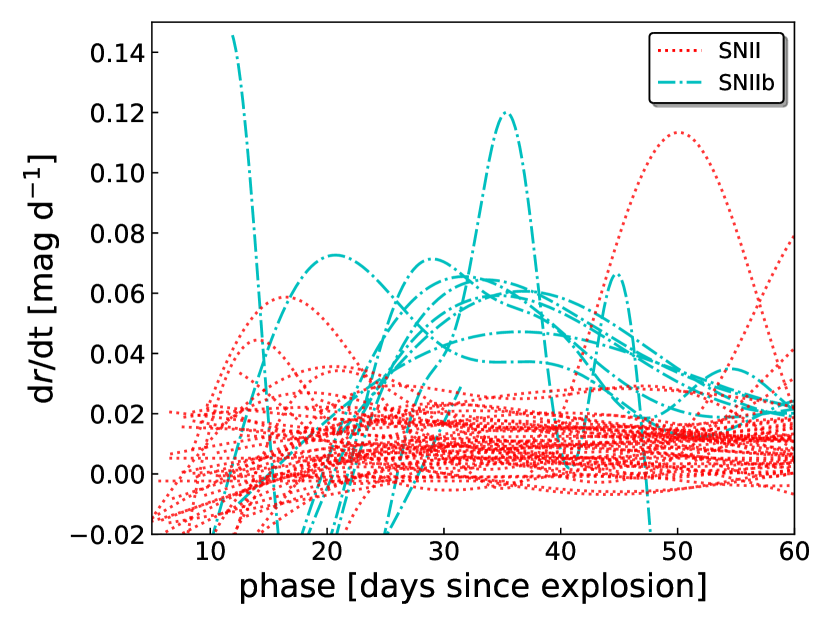
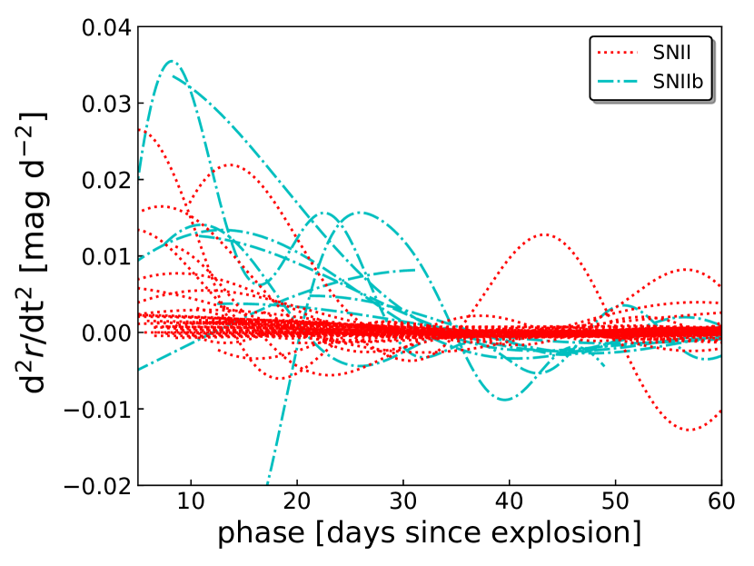
Figure 13: Derivative of the $r$-band light curve with respect to explosion. SNe II are plotted in red dotted lines while SNe IIb are plotted in cyan dash-dot lines. Top panel: first derivative. Bottom panel: second derivative.

To better study the behaviour of the light curves, the continuous resampling was used to compute their time derivatives, which are presented for $V$ band in Fig. 3. Similar plots can be seen for $B$ and $r$ bands in Fig. 12 and Fig. 13 respectively. Finite differences were performed in order to obtain the first and second derivatives of the light curve. Both derivatives of SN II are closer to zero than SN IIb during the first 50 days after explosion, suggesting that their light curve shapes change more slowly than those of SNe IIb during this period of time. Similarly to Fig. 2, Fig. 3 shows that SNe II and SNe IIb separate qualitatively in their derived light curves.

The parameters we define in order to quantitatively compare the light curves are described below:

• $t_{\mathrm{rise}}$: time to maximum light or rise time, considered to be the elapsed time between the date of explosion and the date of maximum light.

• $\Delta m_{40-30}$: magnitude difference between phases 30 and 40 days post explosion, which accounts for the decline rate of the light curve. The phases are chosen in order to capture the post-maximum behaviour of both SN types. This parameter is similar to $\mathrm{dm}_{1}$ defined below in the sense that it measures a slope of the light curve. We include it here because it is easier to visualize and to measure when data are sparse.

• $\mathrm{dm}_{1}$: earliest maximum of the first light-curve derivative after maximum light. This parameter captures the maximum rate at which the light curve declines after peak.

• $\mathrm{dm}_{2}$: earliest minimum of the second light-curve derivative after maximum light. This parameter gives an idea of how much the curvature of the light curve changes in the region where it changes the most.

To be sure that $\mathrm{dm}_{1}$ and $\mathrm{dm}_{2}$ describe the early part of the light curve we add the constraint that $\mathrm{dm}_{1}$ should occur before 80 days (to exclude the decline after the “plateau” of the slow declining SN II) and $\mathrm{dm}_{2}$ should occur after $\mathrm{dm}_{1}$ (to exclude the change in curvature that happens before the main peak of the SN IIb). Some SN II light curves appear nearly as straight lines. In such cases, we do not provide values of $\mathrm{dm}_{1}$ and $\mathrm{dm}_{2}$ since the derivative of a straight line is a constant.

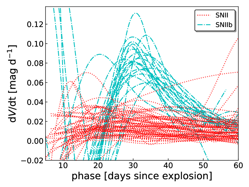
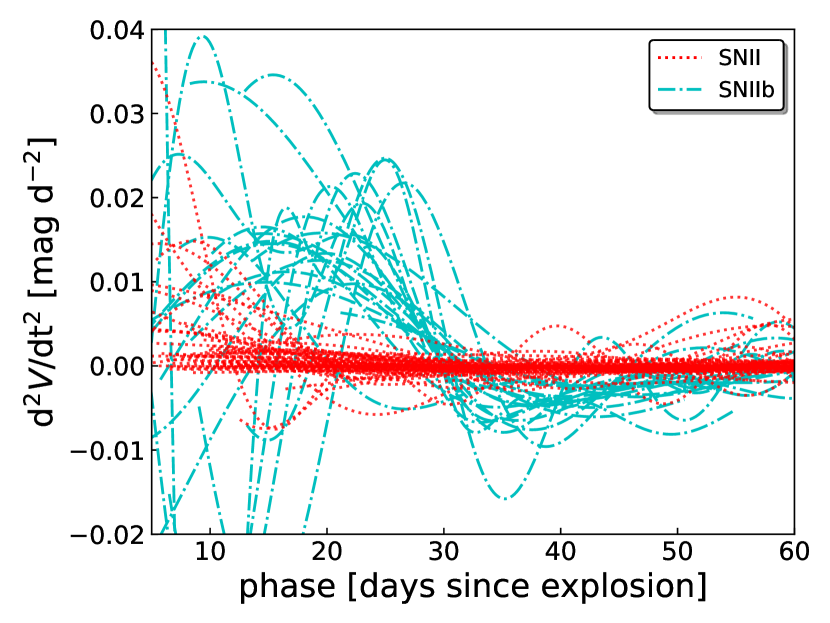
Figure 3: Derivatives of the $V$-band light curves with respect to explosion. SNe II are plotted in red dotted lines while SNe IIb are plotted in cyan dash-dot lines. Top panel: first derivative. Bottom panel: second derivative. Similar trends are observed in the $B$- and $r$-band (see Appendix A).

5 Results

5.1 Rise times

In Fig. 4 we present histograms of $t_{\mathrm{rise}}$ in the three bands considered in this work. We note that while the mean values of the distributions change considerably between bands for SNe II (larger values for longer wavelengths), for SNe IIb the distribution means appear nearly constant (see Table 4). This is expected to happen because, on the one hand, the light-curve maximum of SNe II is attributed to post-shock cooling emission. As the ejecta cools down, the emission peak moves to longer wavelengths and therefore the light-curve maximum is later in redder bands. On the other hand, the light-curve maximum of SNe IIb is thought to be regulated by the diffusion time-scale of ⁵⁶Ni decay radiation, which is nearly constant in the optical. An Ashman’s D test (Ashman et al. 1994) is performed in order to test if there is a possible bimodal behaviour between the distributions of the different parameters, this is accounted for by the D factor. A D value $\geq 2$ suggests bimodality. In this case we obtain $D_{B}\,=\,3.9$, $D_{V}\,=\,2.9$ and $D_{r}\,=\,1.9$, which we interpret as a clear distinction between the $t_{\mathrm{rise}}$ values of both SN types in all three bands. Since the variables under study do not strictly come from Gaussian distributed parent populations, we also performed a Silverman’s test (Silverman 1981) after which two modes can be observed, supporting a distinction between SNe II and SNe IIb.

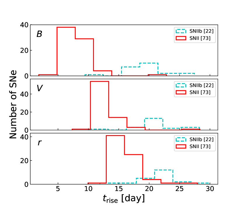
Figure 4: $t_{\mathrm{rise}}$ distributions. $B$-, $V$- and $r$-band from top to bottom. The total number of objects is specified in brackets for each band. SNe II are plotted in red solid lines and SNe IIb in cyan dashed lines.

The weighted average of $t_{\mathrm{rise}}$ is calculated for the three bands (see Table 4), using as weights the errors on $t_{\mathrm{rise}}$. We compared these values with those obtained in previous works.

• Valenti et al. (2016) present for SNe II in their Figure 16 a distribution of $t_{\mathrm{rise}}$ vs. $V$-band magnitude that goes from $\sim$0 days to $\sim$20 days. The mean value of $t_{\mathrm{rise}}$ is $\sim$10 days which is consistent with our result;

• Rubin et al. (2016) present the $t_{\mathrm{rise}}$ of 57 SNe II in the $R$-band (that can be considered similar to $r$-band). From their Table 3 we calculate an average $t_{\mathrm{rise}}$ of 7.74 $\pm$ 2.9 days. Subsequently, Rubin & Gal-Yam (2016) using a similar sample to Rubin et al. (2016) found three groups: fast rise/slow decline (II-FS), fast rise/fast decline (II-FF) and slowly rising (II-S). The first two groups with $t_{\mathrm{rise}}$ $\sim$ 6.5 days and the last one with $t_{\mathrm{rise}}$ $\sim$ 10 days. Furthermore González-Gaitán et al. (2015) find for SNe II a $t_{\mathrm{rise}}$ of 7.5 $\pm$ 0.3 days in the $g$-band (that can be compared to the $V$-band). The distributions of these studies are systematically smaller than what we derive for our sample. The studies mentioned before used photometry from surveys with higher cadence than those producing the majority of our sample data, which could be the origin of these differences.

• Gall et al. (2015) present $t_{\mathrm{rise}}$ of a sample of SNe II in the $r^{\prime}/R$-band. From their Table 4 we calculate an average of $10.14\pm 4.42$ days which is consistent within uncertainties with our values;

• Prentice et al. (2016) present in their Table 7 a list of literature bolometric $t_{\mathrm{rise}}$ values for SE SNe. With the values corresponding to SNe IIb we calculate an average of $15.89\pm 4.8$ days. Considering that we find that $B$-, $V$- and $r$-band light curves for SN IIb reach their maximum at very similar epochs, we can assume that the bolometric light curves also reach their maxima at a similar time. Their bolometric $t_{\mathrm{rise}}$ is smaller than what we find here, although still compatible within the uncertainties;

• Taddia et al. (2015) present in their Table 4 values for SNe IIb $t_{\mathrm{rise}}$ in the $R/r$-band. The resulting average rise time is $23.07\pm 1.96$ days which is consistent with our results;

• A subgroup of our SNe IIb sample is part of the work of Taddia et al. (2018). They present the explosion epoch and the epoch of maximum light in different bands for each object. From this, one can infer the $t_{\mathrm{rise}}$. We calculate an average $t_{\mathrm{rise}}$ for $B$-band of $18.97\pm 2.73$ days, for $V$-band an average of $20.84\pm 2.94$ days and for $r$-band an average of $21.78\pm 3.32$ days which closely match our results.

In summary, the $t_{\mathrm{rise}}$ of SNe IIb are consistently longer than for SNe II, both in the current work and in the literature. Note that the computed $t_{\mathrm{rise}}$ average is bigger for our SN II sample than for other higher cadence samples (see above). While this is a caveat to our estimated $t_{\mathrm{rise}}$ distributions, assuming that our values are slightly overestimated only strengthens our conclusion that SNe IIb have longer $t_{\mathrm{rise}}$ than SNe II.

Table 4: Weighted average and $rms$ of $t_{\mathrm{rise}}$ for every band.

Type	Band	Weighted average
IIb	$B$	19.0 $\pm$ 1.8
	$V$	20.9 $\pm$ 1.6
	$r$	21.3 $\pm$ 2.1
II	$B$	8.3 $\pm$ 2.0
	$V$	12.8 $\pm$ 2.4
	$r$	16.0 $\pm$ 3.6

5.2 Magnitude difference between 40 and 30 days post-explosion

In Fig. 5 we present histograms of $\Delta m_{40-30}$ for the three bands considered in this work. It can be seen in this figure that both SN populations are separated in the sense that SNe IIb have larger $\Delta m_{40-30}$ values, which reflects the fact that SNe IIb decline faster than SNe II after maximum light at these epochs. The Ashman’s D values for this parameter are $D_{B}\,=\,3.0$, $D_{V}\,=\,4.7$ and $D_{r}\,=\,5.6$. The Silverman test also indicates the presence of two modes. These results confirm the visual conclusion that the distributions are bimodal.

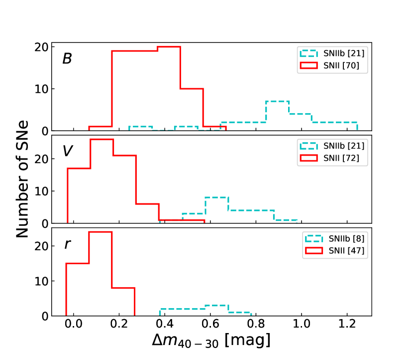
Figure 5: $\Delta m_{40-30}$ distributions. $B$-, $V$- and $r$-band from top to bottom. The total number of objects is specified in brackets for each band. SNe II is plotted in red solid lines and SNe IIb in cyan dashed lines.

5.3 Derivatives

In Fig. 6 we present the distributions of the first maximum of the first derivative ($\mathrm{dm}_{1}$, top panel) and of the first minimum of the second derivative ($\mathrm{dm}_{2}$, bottom panel) both after light curve peak for $B$-, $V$- and $r$-band. It can be seen that generally $\mathrm{dm}_{1}$ is larger for SNe IIb meaning that they decline faster than SNe II. The Ashman’s D calculated for $\mathrm{dm}_{1}$ are: $D_{B}\,=\,4.3$, $D_{V}\,=\,4.2$ and $D_{r}\,=\,4.1$. The Silverman test also indicates the presence of two modes, evidencing two different distributions for this parameter. At the same time it can be observed that $\mathrm{dm}_{2}$ values for SNe IIb are greater in absolute value (i.e., more negative) than those of SNe II. This indicates that the change in curvature after the initial decline is greater for SNe IIb than for SNe II. We obtain $D_{B}\,=\,2.8$, $D_{V}\,=\,2.1$, and $D_{r}\,=\,1.3$. These results imply that there might be only one distribution for $\mathrm{dm}_{2}$ in the $r$-band. However the Silverman test shows two modes for $B$- and $r$-band while showing only one mode for $V$-band, implying that this last band might be the one showing unimodal behaviour. Despite these results, the general shape of the light curves is different between both types of SNe in $V$- and $r$-band.

In general the slope of the decline after the first peak ($\mathrm{dm}_{1}$) of SNe IIb seems to be smaller for redder bands, but this is not so clear for SNe II between $V$- and $r$-band.

5.4 Comparison between parameters

In Fig. 7 we present $\mathrm{dm}_{1}$ vs. $\mathrm{dm}_{2}$ in the $V$-band. There seems to be a correlation between these two parameters with a clear trend of increasing $\mathrm{dm}_{1}$ with decreasing $\mathrm{dm}_{2}$. However, the overlap in this parameter plane is very small between both SN types, indicating their distinct light-curve properties. We do not therefore conclude that this trend implies an underlying connection between SN II and SN IIb.

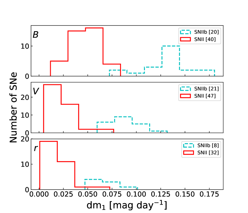
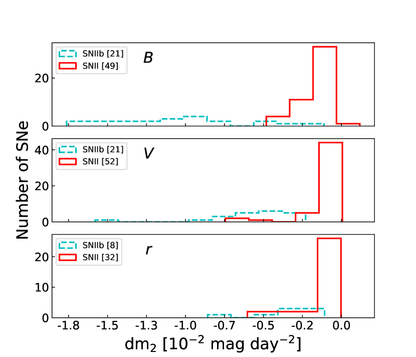
Figure 6: Top: $\mathrm{dm}_{1}$ distributions for all ($B$, $V$ and $r$ from top to bottom) bands. Bottom: $\mathrm{dm}_{2}$ distributions for all ($B$, $V$ and $r$ from top to bottom) bands. The total number of objects is specified in brackets for each band. SNe II are plotted in red solid lines and SNe IIb in cyan dashed lines.

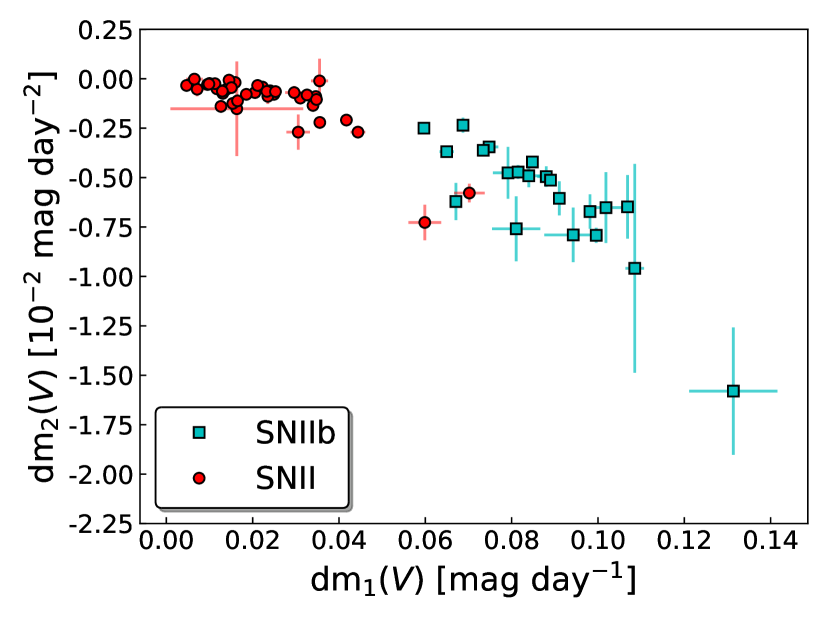
Figure 7: Comparison between $\mathrm{dm}_{1}$ and $\mathrm{dm}_{2}$ in the $V$-band. SNe II are represented by red circles while SNe IIb by cyan squares. Some error bars are smaller than the symbol size.

In Fig. 8 we plot each of the parameters described above against $t_{\mathrm{rise}}$ in $V$-band (see Table 9 for the numeric values of each parameter). In all the panels it can be seen that SN II and SN IIb separate in two groups, with a small number of objects bridging them. These objects are discussed in the next section. We used Gaussian mixture models to performed clustering over these plots in the three studied bands. When plotted out, we see that the ellipses that represent the Gaussian component do not touch. Nevertheless, when studying the $\mathrm{dm}_{2}$ parameter we see that some type II objects fall in the type IIb cluster, these objects are not the same nor the same amount for the different bands, so they are not considered as transitional events. The only systematically “misclassified” object when studying our set of parameters versus $t_{\mathrm{rise}}$ is SN 2013ai, which always appears in the type IIb cluster. SN 2004ff is also “misclassified” for most parameters with the exception of $\mathrm{dm}_{1}$ versus $t_{\mathrm{rise}}$ in the $B$-band.

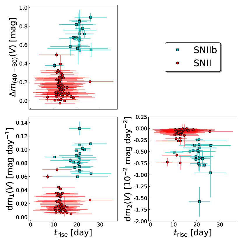
Figure 8: Comparison between parameters in the $V$-band. SNe II are plotted as red circles while SNe IIb are plotted as cyan squares. Top left panel: $\Delta m_{40-30}$ vs. $t_{\mathrm{rise}}$. Bottom left panel: $\mathrm{dm}_{1}$ vs. $t_{\mathrm{rise}}$. Bottom right panel: $\mathrm{dm}_{2}$ vs. $t_{\mathrm{rise}}$.

6 Discussion

We have studied a large sample of hydrogen-rich SN II and SN IIb light curves to test the hypothesis of a continuum of morphological properties among them. Both qualitatively (visually) and quantitatively, SNe II are found to have light curves that are distinct from those of SNe IIb with no suggestion of a continuum of observational properties. Here we discuss the interpretation of our results in terms of the nature of progenitors properties.

6.1 Progenitors

As described in the introduction of this work, it is generally accepted that slow-declining SNe II (IIP) arise from stars that retain a significant fraction ($\gtrsim$ 2${\rm\ M}_{\odot}$, Heger et al. 2003b) of their hydrogen rich envelopes and become red supergiants before exploding. Also, there are suggestions that faster-declining SNe II (IIL) arise from stars that lose a greater fraction of their hydrogen envelopes than slower-declining SNe II. The observed continuum of light-curve decline rates among SNe II may indicate that there is a continuum of progenitor properties, possibly a sequence of envelope masses. At the same time, the spectral transition of SNe IIb from hydrogen dominated to helium dominated in turn suggests that their progenitors retained significantly less hydrogen than the majority of SNe II. Therefore SNe IIb could constitute a continuation of the envelope-mass sequence that is suggested for SNe II. The dominant mass loss mechanism producing these degree of envelope stripping is still a matter of debate.

One explanation could be mass loss via strong winds or eruptions. In this scenario Wolf-Rayet (WR) stars have been considered probable progenitors of SE SNe. However, single stars are only predicted to lose sufficient mass to explode as SE SNe when their initial masses are higher than 25${\rm\ M}_{\odot}$ (see e.g. Heger et al. 2003b). Nevertheless, the rate of SE SNe is significantly higher than that predicted assuming single-star progenitors and a standard initial mass function (IMF, Smith et al. 2011). Also, the ejecta masses of SE SNe are lower than those expected from $>$ 20${\rm\ M}_{\odot}$ progenitors, presenting a problem for single-star progenitors (e.g. Drout et al. 2011, Lyman et al. 2016, Taddia et al. 2018). Nonetheless, recent stellar models using enhanced mass loss suggest that SN IIb (and Ib) could come from stars $\sim$ 20-25${\rm\ M}_{\odot}$ (Chieffi & Limongi 2013). In this case, a single-star progenitor continuum could be considered between slow-declining SNe II (IIP, with the most hydrogen retained by their progenitors), fast-declining SNe II (IIL, with less hydrogen) and SNe IIb (with the least amount of hydrogen left in their progenitors).

In the second and more popular explanation for SNe IIb progenitor’s mass loss, hydrogen envelope stripping is achieved through the presence of a companion. This is supported by the strong evidence that the majority of massive stars reside in interacting binary systems (Sana et al. 2012) and by the observed fractions of supernova types (Smith et al. 2011). While the confirmed progenitors of SNe II are compatible with single-star evolutionary models (Van Dyk 2012, Smartt 2015 and references therein), those of SNe IIb do not comply with this picture and appear to indicate a binary origin. Furthermore, for three SNe IIb there is evidence of a binary companion (SN 1993J Maund et al. 2004, SN 2001ig Ryder et al. 2018 and SN 2011dh Maund et al. 2011, Folatelli et al. 2014).

Progenitor properties can be indirectly studied via the observed properties of the SN light curves. The continuum observed between slow and fast declining SN II light curves has been attributed to a possible continuum of progenitor properties. In this work we do not find evidence for a continuum between the observed properties of hydrogen-rich SN II and SN IIb light curves. This may indicate that these events arise from different progenitor scenarios.

6.1.1 Constraints from hydrodynamical modelling

Using hydrodynamical models one can test whether the hydrogen rich envelope mass is the driving factor that shapes the light curves of SNe II and IIb. Such a test has been carried out by simulating the explosion of stars with varying envelope masses using our own hydrodynamic code (Bersten et al. 2011). A similar study was done by Morozova et al. (2015). We have calculated SN progenitors using the stellar evolution code MESA version 10398 (Paxton et al. 2011, Paxton et al. 2013). An initial mass of 18 and 30${\rm\ M}_{\odot}$ has been adopted, and produced pre-SN objects of different envelope masses by artificially varying the wind efficiency parameter, $\eta$, within the “Dutch” wind scheme (de Jager et al. 1988, Nugis & Lamers 2000, Vink et al. 2001, Glebbeek et al. 2009). We evolved the stellar models from the pre-main-sequence to the time of core collapse, defined as the moment when any part of the core exceeds an infall velocity of 1000 km/s. All pre-SN objects were exploded assuming a fixed energy of 10⁵¹ erg and a radioactive ⁵⁶Ni mass of 0.02${\rm\ M}_{\odot}$. A complete analysis based on these tests is deferred to a future publication, here we briefly describe these results to aid in our discussion and conclusions.

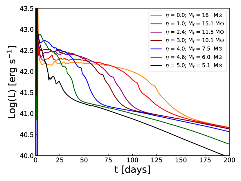
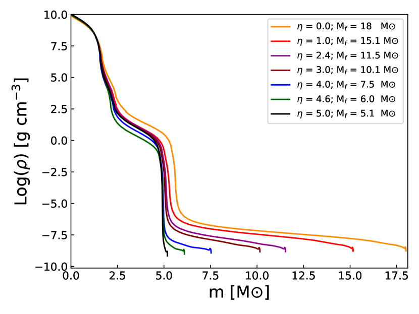
Figure 14: Models of a 18${\rm\ M}_{\odot}$ progenitor with different values of the wind efficiency ($\eta$), considering an explosion energy of 1 foe and ⁵⁶Ni mass of 0.02${\rm\ M}_{\odot}$. A model without mass loss by winds ($\eta$=0.0) is shown for comparison. M_f denotes the final mass (pre-explosion) of the progenitor. Top panel: Bolometric light curves. Bottom panel: Initial density profiles.

The resulting light curves (Fig. 14) are similar to those in Morozova et al. 2015 (see their Fig. 7). However, our conclusions are distinct. We note that as the envelope mass decreases, the light curves decline faster during the recombination phase. This is in line with the range of SN II light-curve morphologies from “plateau” to “linear”. When the envelope mass falls below 0.5${\rm\ M}_{\odot}$  the light curves show a bump that Morozova et al. (2015) interpret as a signature of SNe IIb. However, the properties of the computed light curves differ substantially from those of observed SNe IIb. The bump luminosity is too low, and its timing and duration are too short to account for the observed SNe IIb light curves. Also, the duration of the cooling phase preceding the bump is not compatible with observations. Our interpretation is that the envelope mass regulates on the zeroth order the shape of SN II light curves, but it cannot account for SNe IIb. Although, for the latter, there is evidence that a difference of $\sim$0.1${\rm\ M}_{\odot}$ of hydrogen in the envelope divides SN IIb into two categories: those with a compact progenitor (SN cIIb) and those with an extended one (SN eIIb, Chevalier & Soderberg 2010). Further investigation of this phenomenon is beyond the scope of this work.

A recent population synthesis study of binary systems combined with explosion models presented by Eldridge et al. (2018) claims that the variety of progenitor systems can produce a continuum of light-curve shapes including SNe II (plateau and linear) and SNe IIb. However, the synthetic light curves that they classify as of Type IIb do not comply with the observed properties (similarly to above). As seen in their Fig. 4, the SN IIb models are too faint in general, and while some light curves are too wide, others peak too early or show a peculiar initial peak. Previous studies have shown that in order to reproduce the light-curve shapes of SNe IIb, the outermost density structure of the progenitor needs to be modified relative to those of standard evolutionary models (see Fig. 1 in Bersten et al. 2012).

We conclude that the observed discontinuity in light-curve morphology between SNe II and SNe IIb must involve progenitor properties in addition to the mass of the hydrogen rich envelope. Further analysis is required to elucidate what such properties are and what the role of binarity is in determining them.

6.2 SNe II light-curve morphology: a clear continuum

As mentioned in Sec. 1, most contemporary work on samples of SNe II (this refers to all those events historically classified as IIP and IIL) conclude that a continuum exists between the slowest declining SNe II and the faster declining events. While here our aim was not to further explore the IIP-IIL classification, it is clear that in all of our measured parameters - that are distinct from those defined in previous works, see e.g. Anderson et al. (2014) - there is no evidence for bimodality. This work therefore further supports the existence of a continuum in the properties of slow and fast declining SNe II.

6.3 Possible transitional/outlying events

All of the qualitative and quantitative results and discussion we have presented so far have concluded that there is no clear continuum in light-curve properties between hydrogen-rich SNe II and SNe IIb. However, in several figures (see Fig. 7 and 8) there are a small number of SNe that appear to bridge the two populations. In this subsection we investigate whether any of these events could be considered transitional by studying their photometric and spectroscopic properties in more detail.

6.3.1 Type II

• SN 2013ai: This is the most noticeable SN II outlier since it has an exceptionally large $t_{\mathrm{rise}}$ when compared to the rest of our SNe II sample, it is also the only systematically “misclassified” object when performing a clustering analysis. We have checked that none of the other parameters considered indicated this object belonged to the SN IIb group, meaning that the behaviour of the light curve (steepness and decline rate after peak) is otherwise typical of SNe II. Nevertheless, we have inspected its spectra for similarities to SNe IIb. None are found, and SN 2013ai also shows typical spectral features and spectral evolution to those of SNe II. Therefore we consider it to be a spectroscopically normal SN II with a slow rise. Rubin & Gal-Yam (2016) study 59 SNe II in the $R$-band. They find three different clusters of objects, one only composed of slowly rising events (II-S cluster). However, their II-S sample have a median $t_{\mathrm{rise}}$ of  10 days while SN 2013ai has a $t_{\mathrm{rise}}$ of 25.5$\pm$10.5 days in the $r$-band. Therefore (even considering the error) the $t_{\mathrm{rise}}$ of SN 2013ai is still significantly longer than that of the II-S. This object is further analyzed by Davis et al. (in preparation).

• SN 2006Y: This SN has large $\mathrm{dm}_{1}$ and $\mathrm{dm}_{2}$ values when compared to the rest of the SNe II sample. SN 2006Y is an outlier on the observed trends of the Anderson et al. (2014) sample: they find it to be the fastest decliner of their sample; this SN is again an outlier in the sample of Gutiérrez et al. (2014), showing the smallest H$\alpha$ absorption of their sample. However, its $t_{\mathrm{rise}}$ is typical of SNe II and its light curve has a small “plateau” a few days after peak that is not observed in any SNe IIb. Also it shows strong hydrogen lines throughout its spectral evolution. Therefore, while SN 2006Y shows abnormal properties for a SN II, these do not position this event close to the parameter space of SNe IIb.

• SN 2013fs: This object also has large $\mathrm{dm}_{1}$ and $\mathrm{dm}_{2}$, when compared to the rest of the SNe II sample. In all other parameters ($t_{\mathrm{rise}}$, $\Delta m_{40-30}$, overall shape of the light curve, spectral evolution) it behaves as a normal SN II.

• SN 2008M: This SN does not present any peculiarities except for a large $\mathrm{dm}_{2}$. While visual inspection of its light curve shows an early fast decline, later it has a normal “plateau” lasting for approximately 80 days. In no other parameter does this event appear similar to SNe IIb.

6.3.2 Type IIb

• SN 2004ff: This SN has an unusually small $t_{\mathrm{rise}}$ value. Checking our estimated time of maximum light we find that it is in agreement with that from Taddia et al. (2018). However, investigating the pre-discovery non-detection values this SN may have a poorly constrained explosion epoch. This conclusion arises from the fact that the non-detection limiting magnitude is 18 mag (Oct. 21.4) while the discovery magnitude is 17.8 mag (Oct. 28.39, Pugh et al. 2004). Such a shallow non-detection may not give an accurate constraint on the explosion epoch. If we consider the explosion epoch obtained with SNID - which agrees within uncertainties with that obtained by Taddia et al. (2018) via a fit to the photospheric radius before $r_{\mathrm{max}}$ - the $t_{\mathrm{rise}}$ agrees with that of the rest of the SNe IIb sample. Examining the other parameters defined in this work we notice that $\Delta m_{40-30}$ seems to be positioning this object among SNe II but not $\mathrm{dm}_{1}$. These two parameters account for steepness of the light curve but $\mathrm{dm}_{1}$ is independent of the explosion epoch and thus it is not affected by any possible error in the determination of the explosion epoch. The value of $\mathrm{dm}_{2}$ for SN 2004ff is consistent with the rest of the SN IIb population. Finally, if the explosion epoch is wrong, the light curve would look like those of typical SNe IIb (with typical $t_{\mathrm{rise}}$ and $\Delta m_{40-30}$), but shifted in time. Therefore we conclude that it is not a transitional event.

6.3.3 The Type II SN 2001fa and Type II(?) SN 2007fz

These two objects are not included in our sample but they are in the Faran et al. (2014) sample. Those authors studied 11 fast declining hydrogen-rich SNe II and argued that SN 2001fa and SN 2007fz (shown in their Figure 8) could be transitional events between SNe II and SNe IIb. Given that within our sample we find a lack of transitional events, we decided to examine these two SNe in more detail. In Fig. 9 the light curves of SN 2001fa and SN 2007fz are plotted in comparison to the SN II and SN IIb samples analyzed in our work.

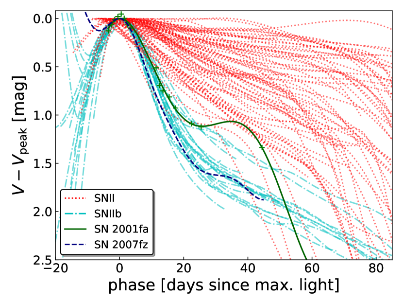
Figure 9: Resampled light curves normalized with respect to the $V$-band peak magnitude, SNe II are plotted in red dotted lines while SNe IIb are plotted in cyan dash-dot lines. In green solid lines is SN 2001fa (the photometric data points were added as green crosses to show the sparse sampling after 20 days) and in blue dashed lines SN 2007fz.

The resampled light curve of SN 2001fa appears to be more consistent with the overall morphology of SN II than SN IIb light curves, showing a small “plateau” (however the cadence of the photometry at these epochs is not optimal). In addition, according to SNID SN 2001fa is consistent with it being a SN II, and therefore we conclude that this is not a transitional event.

The resampled shape of the light curve of SN 2007fz is compatible with those of SNe IIb. The $V$-band rise time (18.2 days) is also consistent with SNe IIb. Regarding the spectra, Faran et al. (2014) argued that they were similar to those of SNe II. To test this we decided to run the four available spectra through SNID (after removing the narrow emission lines of host galaxy contamination). The SNID classification output is not conclusive as for the first three spectra the best match is a SN IIb, while for the last one the best match is a SN II. We further examined this last SNID classification output and notice that the SNe II templates match quite well the H$\alpha$ emission for the studied spectra but they do not match the H$\alpha$ absorption nor the He lines. On the contrary, the SNe IIb templates show an additional dip in the H$\alpha$ emission that is not seen on the studied spectra (as described by Faran et al. 2014) but, match well both the H$\alpha$ absorption and the He lines. We conclude that SN 2007fz is most probably a Type IIb SN and not a SN II (as claimed by Faran et al. 2014).

6.4 SNe IIb without observed maxima

In Section 1 it is stated that only SNe IIb with data points around maximum are considered. This could introduce a sample bias because there may be SNe IIb with shorter rise times where the rise was not observed because it occurred sooner after explosion. Therefore, we searched the Open Supernova Catalog (Guillochon et al. 2017) for SNe IIb that met the same criteria we use to select our sample but without observed photometric data points around maximum light. We found two objects (see Table 8) that satisfied these requirements. The explosion epoch and date of maximum light were obtained by spectral matching using SNID as described in Sections 3.1 and 3.2. The mean $t_{\mathrm{rise}}$ for these objects $V$-band is 19.6 days, which is consistent with our results. Even though these are only two examples, the result suggests that our photometric selection criteria are not driving our results on the significant differences in rise times between SNe II and SNe IIb.

7 Conclusions

We present a morphological analysis of $B$-, $V$- and $r$-band light curves for 95 SNe (73 SNe II and 22 SNe IIb). Overall, we conclude that the two samples show distinct light-curve shapes and seem to form a bimodal distribution in all the defined parameters. In the $V$-band a $t_{\mathrm{rise}}$ of 17d, $\Delta m_{40-30}$ of 0.4mag, $\mathrm{dm}_{1}$ of 0.05mag$\cdot$day^-1 and $|\mathrm{dm}_{2}|$ of 0.003mag$\cdot$day^-2 serve as an approximate threshold between both types of SNe. In the $B$-band these thresholds are $t_{\mathrm{rise}}$ $=$ 13.7d, $\Delta m_{40-30}$ $=$ 0.6mag, $\mathrm{dm}_{1}$ $=$ 0.09mag$\cdot$day^-1 and $|\mathrm{dm}_{2}|$ $=$ 0.006mag$\cdot$day^-2. Finally in the $r$-band, $t_{\mathrm{rise}}$ $=$ 18.8d, $\Delta m_{40-30}$ $=$ 0.3mag, $\mathrm{dm}_{1}$ $=$ 0.04mag$\cdot$day^-1 and $|\mathrm{dm}_{2}|$ $=$ 0.002mag$\cdot$day^-2 can be used as thresholds, with lower values corresponding to SNe II and higher (absolute) values corresponding to SNe IIb.

These results argue against a continuum of observed properties between SN II an SN IIb. Our main conclusions are:

• The clear separation seen between both SN types suggests that they may arise from distinct progenitor channels. Alternatively, even if they share a common origin, there must be a physical property (or a combination thereof) that under a continuum variation produces a sudden change in the resulting SN properties.

• All the studied parameters are on average larger for SNe IIb. Larger $\mathrm{dm}_{1}$ indicates that their post peak decline is steeper than that of SNe II. Larger $|\mathrm{dm}_{2}|$ indicates that their change after the first decline post maximum is more pronounced than that of SNe II.

• Our findings agree with the recent claims that SNe II form a single continuous family (Anderson et al. 2014, Sanders et al. 2015, Galbany et al. 2016, Rubin & Gal-Yam 2016). They also agree with the observed separation between SNe II and IIb previously suggested by Arcavi et al. (2012) and hinted by Rubin & Gal-Yam (2016) when they mention that the outliers in their SNe II study are consistent with type IIb objects.

Appendix A Additional results

Table 5: SNe II sample (same in other tables). References: (1^p) Leonard et al. (2002); (2^p) Galbany et al. (2016); (3^p) Anderson et al. (2014) and Contreras et al. in prep.; (4^p) Takáts et al. (2015); (5^p) Dall’Ora et al. (2014); (6^p) Valenti et al. (2016); (7^p) Valenti et al. (2015); (8^p) Yuan et al. (2016); (9^p) Huang et al. (2016); (10^p) Terreran et al. (2016). (1^s) WISeREP (Yaron & Gal-Yam 2012); (2^s) Gutiérrez et al. (2017a);(3^s) Leonard et al. (2002);(4^s) Shivvers et al. (2017); (5^s) Takáts et al. (2015); (6^s) Dall’Ora et al. (2014); (7^s) Childress et al. (2016); (8^s) Valenti et al. (2015); (9^s) Black et al. (2017); (10^s) Yuan et al. (2016); (11^s) Valenti et al. (2014); (12^s) Dhungana et al. (2016); (13^s) Bose et al. (2015); (14^s) Yaron et al. (2017);(15^s) Terreran et al. (2016).

SN	z_host	Exp[MJD]	V_Max[MJD]	B_Max[MJD]	r_Max[MJD]	Phot. Ref.	Spec. Ref	Circular
1999gi	0.0020	51518.2(3.7)	51529.2(2.2)	51526.3(2.1)	51532.2d (3.4)	(1p)	(1s);(3s);(4s)	IAUC 7329
2002fa	0.0600	52502.5a (8.0)	52515.9c (4.6)	52510.9d (5.0)	52518.9d (5.3)	(2p)	(2s)	IAUC 7967
2002gd	0.0089	52551.5a (4.0)	52562.6(2.3)	52558.9(2.7)	52565.6d (3.5)	(2p)	(2s)	IAUC 7986
2002gw	0.0103	52553.5a (8.0)	52572.0c (4.7)	52567.0d (5.2)	52575.0d (5.4)	(2p)	(2s)	IAUC 7995
2002hj	0.0236	52562.5a (7.0)	52575.5c (5.6)	52570.5d (6.0)	52578.5d (6.2)	(2p)	(2s)	IAUC 8006
2002hx	0.0310	52582.5a (9.0)	52595.4c (5.6)	52590.4d (6.0)	52598.5d (6.2)	(2p)	(2s)	IAUC 8015
2002ig	0.0770	52570.5a (5.0)	52584.7c (3.6)	52579.6d (4.2)	52587.7d (4.5)	(2p)	(2s)	IAUC 8020
2003bl	0.0146	52696.5a (4.0)	52711.2c (5.0)	52706.2d (5.4)	52714.2d (5.6)	(2p)	(2s)	IAUC 8086
2003bn	0.0128	52694.5a (3.0)	52707.1c (4.0)	52702.1d (4.5)	52710.1d (4.8)	(2p)	(2s)	IAUC 8088
2003ci	0.0304	52711.5a (8.0)	52723.8c (4.5)	52718.8d (5.0)	52726.9d (5.3)	(2p)	(2s)	IAUC 8097
2003cn	0.0181	52717.5a (4.0)	52731.5c (4.5)	52726.5d (5.0)	52734.6d (5.2)	(2p)	(2s)	IAUC 8101
2003cx	0.0370	52725.5a (5.0)	52740.4c (4.1)	52735.4d (4.7)	52743.5d (4.9)	(2p)	(2s)	IAUC 8105
2003ef	0.0139	52757.5a (9.0)	52771.8c (4.8)	52766.8d (5.3)	52774.9d (5.5)	(2p)	(2s)	IAUC 8131
2003fb	0.0175	52772.5a (10.0)	52788.9c (5.1)	52783.9d (5.5)	52791.9d (5.8)	(2p)	(2s)	IAUC 8143
2003hd	0.0395	52855.9a (5.0)	52870.1c (4.2)	52865.1d (4.7)	52873.1d (5.0)	(2p)	(2s)	IAUC 8179
2003hg	0.0143	52865.5a (5.0)	52877.7c (5.9)	52872.6d (6.3)	52880.7d (6.5)	(2p)	(2s)	IAUC 8184
2003hl	0.0082	52868.5a (5.0)	52881.8c (4.0)	52876.8d (4.5)	52884.8d (4.8)	(2p)	(2s)	IAUC 8184
2003hn	0.0039	52866.5a (10.0)	52879.1c (4.6)	52874.1d (5.1)	52882.2d (5.3)	(2p)	(2s)	IAUC 8186
2003ib	0.0248	52891.5a (8.0)	52902.7c (3.5)	52897.7d (4.1)	52905.8d (4.4)	(2p)	(2s)	IAUC 8201
2003ip	0.0180	52896.5a (4.0)	52908.2c (5.4)	52903.2d (5.8)	52911.3d (6.0)	(2p)	(2s)	IAUC 8214
2003iq	0.0082	52919.5a (2.0)	52931.8c (4.7)	52926.8d (5.2)	52934.9d (5.4)	(2p)	(2s)	CBET 48
2003E	0.0147	52629.5a (8.0)	52647.0c (4.1)	52642.0d (4.6)	52650.0d (4.9)	(2p)	(2s)	IAUC 8044
2003T	0.0279	52654.5a (10.0)	52668.0c (5.3)	52662.9d (5.7)	52671.0d (5.9)	(2p)	(2s)	IAUC 8058
2004er	0.0147	53271.8a (2.0)	53287.6(1.8)	53282.6(1.9)	53292.9(1.6)	(3p)	(2s)	CBET 93
2004fc	0.0061	53293.5a (1.0)	53306.5c (5.3)	53301.4d (5.7)	53309.5d (5.9)	(3p)	(2s)	IAUC 8422
2004fx	0.0089	53303.5a (4.0)	53316.2c (5.2)	53311.2d (5.6)	53319.2d (5.8)	(3p)	(2s)	IAUC 8431
2005an	0.0107	53431.8a (6.0)	53444.8c (4.5)	53439.8d (5.0)	53447.8d (5.2)	(3p)	(2s)	CBET 113
2005dt	0.0257	53605.6a (9.0)	53616.4c (3.9)	53611.4d (4.5)	53619.4d (4.7)	(3p)	(2s)	CBET 213
2005dx	0.0267	53611.8a (7.0)	53625.9c (5.0)	53620.9d (5.4)	53629.0d (5.7)	(3p)	(2s)	CBET 220
2005dz	0.0190	53619.5a (4.0)	53632.2c (4.4)	53627.2d (4.9)	53635.3d (5.1)	(3p)	(2s)	CBET 222
2005lw	0.0257	53716.8a (10.0)	53729.2c (3.7)	53724.2d (4.3)	53732.3d (4.6)	(3p)	(2s)	CBET 318
2005me	0.0224	53717.9a (10.0)	53730.3c (4.2)	53725.3d (4.7)	53733.3d (5.0)	(3p)	(2s)	CBET 333
2005J	0.0139	53379.8a (7.0)	53392.5c (5.1)	53387.5d (5.5)	53395.6d (5.8)	(3p)	(2s)	IAUC 8467
2005K	0.0274	53369.8a (8.0)	53382.5c (4.4)	53377.4d (4.9)	53385.5d (5.1)	(3p)	(2s)	IAUC 8468
2005Z	0.0192	53396.7a (6.0)	53409.4c (4.7)	53404.4d (5.1)	53412.5d (5.4)	(3p)	(2s)	IAUC 8476
2006ai	0.0152	53781.6a (5.0)	53793.7c (4.9)	53788.6d (5.4)	53796.7d (5.6)	(3p)	(2s)	CBET 406
2006be	0.0071	53802.8a (9.0)	53816.0c (5.9)	53810.9d (6.3)	53819.0d (6.5)	(3p)	(2s)	CBET 449
2006bl	0.0324	53822.7a (10.0)	53835.9c (6.5)	53830.9d (6.9)	53839.0d (7.0)	(3p)	(2s)	CBET 597
2006ee	0.0154	53961.9a (4.0)	53975.0c (5.0)	53969.9d (5.4)	53978.0d (5.7)	(3p)	(2s)	CBET 597
2006iw	0.0308	54010.7a (1.0)	54022.6c (4.2)	54017.5d (4.7)	54025.6d (4.9)	(3p)	(2s)	CBET 663
2006qr	0.0145	54062.8a (7.0)	54075.7c (4.7)	54070.6d (5.2)	54078.7d (5.4)	(3p)	(2s)	CBET 766
2006Y	0.0336	53766.5a (4.0)	53777.9c (4.9)	53772.9d (5.3)	53781.0d (5.6)	(3p)	(2s)	IAUC 8668
2007hm	0.0251	54336.6a (6.0)	54348.9c (4.3)	54343.9d (4.8)	54351.9d (5.1)	(3p)	(2s)	CBET 1050
2007il	0.0215	54349.8a (4.0)	54363.7c (5.3)	54358.7d (5.8)	54366.8d (6.0)	(3p)	(2s)	CBET 1062
2007ld	0.0250	54376.5a (8.0)	54388.5c (3.9)	54383.5d (4.4)	54391.5d (4.7)	(3p)	(2s)	CBET 1098

Table 6: continued

SN	z_host	Exp[MJD]	V_Max[MJD]	B_Max[MJD]	r_Max[MJD]	Phot. Ref.	Spec. Ref	Circular
2007oc	0.0048	54388.5a (3.0)	54401.0c (5.4)	54396.0d (5.8)	54404.0d (6.0)	(3p)	(2s)	CBET 1114
2007od	0.0058	54400.6a (5.0)	54412.5c (3.5)	54407.5d (4.1)	54415.5d (4.4)	(3p)	(2s)	CBET 1116
2007P	0.0408	54118.7a (5.0)	54131.3c (5.3)	54126.3d (5.8)	54134.4d (6.0)	(3p)	(2s)	CBET 819
2007U	0.0260	54133.6a (6.0)	54144.9(3.3)	54140.7(3.3)	54150.1(4.8)	(3p)	(2s)	CBET 835
2007W	0.0097	54130.8a (7.0)	54142.9c (4.6)	54137.8d (5.1)	54145.9d (5.3)	(3p)	(2s)	CBET 844
2007X	0.0095	54143.5a (5.0)	54156.3c (4.9)	54151.3d (5.4)	54159.3d (5.6)	(3p)	(2s)	CBET 844
2008bh	0.0145	54543.5a (5.0)	54556.5c (5.2)	54551.4d (5.6)	54559.5d (5.8)	(3p)	(2s)	CBET 1311
2008br	0.0101	54555.7a (9.0)	54567.0c (3.4)	54562.0d (4.0)	54570.1d (4.3)	(3p)	(2s)	CBET 1332
2008bu	0.0221	54566.8a (7.0)	54578.0c (3.0)	54573.0d (3.7)	54581.1d (4.0)	(3p)	(2s)	CBET 1341
2008gi	0.0244	54742.7a (9.0)	54755.0c (5.0)	54749.9d (5.4)	54758.0d (5.6)	(3p)	(2s)	CBET 1539
2008ho	0.0103	54792.7a (5.0)	54805.0c (3.9)	54800.0d (4.5)	54808.0d (4.8)	(3p)	(2s)	CBET 1587
2008if	0.0115	54807.8a (5.0)	54821.4c (4.7)	54816.4d (5.1)	54824.5d (5.4)	(3p)	(2s)	CBET 1619
2008in	0.0052	54825.4a (2.0)	54838.5c (5.4)	54833.4d (5.9)	54841.5d (6.1)	(3p)	(2s)	CBET 1636
2008K	0.0267	54475.5a (6.0)	54487.3c (4.7)	54482.3d (5.2)	54490.4d (5.4)	(3p)	(2s)	CBET 1211
2008M	0.0076	54471.7a (9.0)	54484.6c (5.5)	54479.6d (5.9)	54487.6d (6.1)	(3p)	(2s)	CBET 1214
2009aj	0.0096	54880.5a (7.0)	54893.3c (2.5)	54888.3d (3.3)	54896.4d (3.7)	(3p)	(2s)	CBET 1704
2009ao	0.0111	54890.7a (4.0)	54903.9c (6.0)	54898.9d (6.4)	54906.9d (6.6)	(3p)	(2s)	CBET 1711
2009au	0.0094	54897.5a (4.0)	54909.3c (3.3)	54904.2d (4.0)	54912.3d (4.3)	(3p)	(2s)	CBET 1719
2009bz	0.0108	54915.8a (4.0)	54926.8c (3.5)	54921.7d (4.1)	54929.8d (4.4)	(3p)	(2s)	CBET 1748
2009ib	0.0043	55045.0c (7.6)	55057.1(1.6)	55052.1d (2.7)	55060.1d (3.1)	(4p)	(1s);(5s)	CBET 1902
2009N	0.0034	54846.8a (5.0)	54859.8c (4.4)	54854.8d (4.9)	54862.9d (5.2)	(3p)	(2s)	CBET 1670
2012aw	0.0026	56002.0(0.5)	56012.5(0.6)	56007.5(2.2)	56015.5(2.7)	(5p)	(1s);(6s)	CBET 3054
2013ai	0.0091	56339.7(10.0)	56365.4(1.0)	56359.9(0.9)	56365.2(1.4)	(6p)	(1s);(7s)	ATel 4849
2013by	0.0038	56401.0b (5.0)	56414.7(1.1)	56411.7(1.0)	56414.8(1.0)	(7p)	(1s);(7s);(8s);(9s)	CBET 3506
2013ej	0.0022	56497.5(0.9)	56510.4(0.9)	56508.7(0.9)	56515.9(1.0)	(8p)	(1s);(7s);(10s)	CBET 3606
							(11s);(12s);(13s)
2013fs	0.0118	56570.8(0.5)	56578.1(2.0)	56572.6(1.7)	56580.7(1.5)	(6p)	(1s);(7s);(14s)	CBET 3671
2014cx	0.0055	56901.9(0.5)	56917.5(0.6)	56910.3(0.2)	56925.2(2.3)	(9p)	(1s);(7s)	CBET 3963
2014G	0.0045	56669.6(1.7)	56681.7(0.8)	56678.9(0.7)	56684.6(1.6)	(10p)	(1s);(15s)	CBET 3787

• Notes: SN names (same in other tables) are listed in column 1. In column 2 the heliocentric redshift of the host obtained from NASA/IPAC Extragalactic Database (NED). In column 3 the explosion epoch of the SN and its error obtained from non-detections unless stated differently (see Sec. 3.1). In columns 4, 5 and 6 the epoch of maximum light of the SN light curve and its error in $V$-, $B$- and $r$-band respectively obtained from the light curve unless stated differently (see Sec. 3.2). In column 7 photometry references. In column 8 spectral references. Finally in column 9 is the reference of the discovery circular.

  • Explosion epoch from Gutiérrez et al. (2017a).

  • Explosion epoch estimation from spectral matching.

  • Maximum light epoch from spectral matching.

  • Maximum light epoch with respect to average in $V$-band from those SNe that have data points around maximum, see Table 3).

Table 7: SNe IIb sample. References:(1^p) Stritzinger et al. (2018); (2^p) The Open Supernova Catalog (Guillochon et al. 2017); (3^p) Morales-Garoffolo et al. (2014), Morales-Garoffolo et al. (2015a); (4^p) Bersten et al. (2018); (5^p) Bianco et al. (2014); (6^p) Brown et al. (2014); (7^p) Okyudo et al. (1993) ; (8^p) van Driel et al. (1993); (9^p) Benson et al. (1994); (10^p) Richmond et al. (1994); (11^p) Metlova et al. (1995); (12^p) Barbon et al. (1995); (13^p) Richmond et al. (1996); (14^p) Qiu et al. (1999);(15^p) Galbany et al. (2016);(16^p) Drout et al. (2011);(17^p) Tsvetkov et al. (2009);(18^p) Pastorello et al. (2008);(19^p) Ergon et al. (2014);(20^p) Kumar et al. (2013);(21^p) Morales-Garoffolo et al. (2015b);(22^p) Bufano et al. (2014). (1^s) Yaron & Gal-Yam (2012); (2^s) Holmbo et al. in prep.; (3^s) Matheson et al. (2000); (4^s) Barbon et al. (1995); (5^s) Jerkstrand et al. (2015); (6^s) Modjaz et al. (2014); (7^s) Hamuy et al. (2009); (8^s) Pastorello et al. (2008); (9^s) Taubenberger et al. (2011); (10^s) Oates et al. (2012); (11^s) Arcavi et al. (2011); (12^s) Ergon et al. (2014); (13^s) Ergon et al. (2015); (14^s) Milisavljevic et al. (2013);(15^s) Kumar et al. (2013); (16^s) Morales-Garoffolo et al. (2015b); (17^s) Bufano et al. (2014); (18^s) Childress et al. (2016); (19^s) Szalai et al. (2016); (20^s) Kilpatrick et al. (2017); (21^s) Shivvers et al. (2019)

SN	z_host	Exp[MJD]	V_Max[MJD]	B_Max[MJD]	r_Max[MJD]	Phot. Ref.	Spec. Ref	Circular
1993J	-0.0001	49071.7(2.6)	49095.0(0.1)	49093.7(0.1)	49095.6b (0.8)	(2p);(7p);(8p);	(1s);(3s);	IAUC 5740
						(9p);(10p);(11p);	(4s);(5s)
						(12p);(13p)
1996cb	0.0024	50424.3(8.3)	50450.4(1.8)	50450.4(1.9)	50451.0b (2.0)	(2p);(14p)	(1s);(6s)	IAUC 6524
2003bg	0.0046	52697.3a (7.9)	52717.6(10.3)	52713.6(6.6)	52718.2b (10.4)	(2p);(15p)	(1s);(7s)	IAUC 8082
2004ex	0.0175	53288.8(0.5)	53307.2(1.8)	53306.1(1.5)	53307.8(1.6)	(1p)	(2s)	IAUC 8418
2004ff	0.0226	53302.9(3.5)	53313.1(1.9)	53312.3(1.9)	53314.8(1.5)	(1p)	(6s);(21s)	IAUC 8425
2006ba	0.0191	53802.0a (5.9)	53823.1(1.6)	53821.8b (1.6)	53823.7b (1.7)	(1p);(5p)	(1s);(2s)	CBET 443
2006el*	0.0170	53962.8(0.5)	53983.8(1.6)	53982.5b (1.6)	53984.4b (1.8)	(2p);(5p);(16p)	(1s);(6s)	CBET 605
2006T	0.0081	53759.0(7.0)	53780.3(1.7)	53779.2(1.5)	53781.6(1.9)	(1p);(5p)	(2s);(6s)	IAUC 8666
2008aq	0.0080	54514.9(8.5)	54532.0(1.3)	54530.5(1.3)	54529.9(5.0)	(1p);(5p);(6p)	(2s);(6s)	CBET 1271
2008ax	0.0019	54528.3(0.1)	54549.6(0.5)	54547.9(0.6)	54550.2b (0.9)	(2p);(6p);	(1s);(6s);	CBET 1286
						(17p);(18p)	(8s);(9s)
2008bo	0.0049	54546.4a (4.4)	54567.6(1.2)	54566.6(1.2)	54568.2b (1.4)	(2p);(5p);(6p)	(1s);(6s)	CBET 1324
2009mg	0.0076	55167.6a (7.0)	55188.5(2.0)	55187.2(2.0)	55189.1b (2.2)	(2p);(6p)	(1s);(10s)	CBET 2071
2009K	0.0117	54843.6(1.5)	54869.4(2.4)	54866.9(2.4)	54871.2(2.6)	(1p)	(2s)	CBET 1663
2009Z	0.0251	54858.5a (6.3)	54877.7(2.4)	54876.6(2.7)	54879.0(3.2)	(1p)	(2s)	CBET 1685
2010jr	0.0124	55509.2(2.9)	55531.7(1.6)	55530.2(1.4)	55532.3b (1.8)	(2p);(6p)	-	CBET 2545
2011dh	0.0015	55712.4(0.5)	55732.1(0.9)	55729.8(0.8)	55732.8(1.2)	(2p);(19p)	(1s);(11s)	CBET 2736
							(12s);(13s)
2011ei	0.0093	55763.5a (3.6)	55784.4(0.9)	55782.5(0.9)	55785.0b (1.2)	(2p);(6p)	(1s);(14s)	CBET 2777
2011fu	0.0185	55824.7a (4.2)	55846.0(0.5)	55845.5(0.6)	55846.6b (0.9)	(2p);(20p);(21p)	(1s);(15s);(16s)	CBET 2827
2011hs	0.0057	55867.2a (3.1)	55888.2(0.7)	55884.9(0.7)	55888.8b (1.1)	(2p);(6p);(22p)	(1s);(17s)	CBET 2902
2013ak	0.0034	56349.1a (7.1)	56368.8(1.8)	56366.1(1.8)	56369.4b (1.9)	(2p);(6p)	(1s)	CBET 3437
2013df	0.0024	56443.9(6.9)	56469.8(0.4)	56468.8(0.4)	56470.5(1.3)	(2p);(3p);(6p)	(1s);(18s);(19s)	CBET 3557
2016gkg	0.0049	57651.2(0.1)	57671.7(1.9)	57670.5(1.9)	57672.3b (2.1)	(4p)	(1s);(20s)	vsnet 20188

• Notes: SN names are listed in column 1. In column 2 the heliocentric redshift of the host obtained from NASA/IPAC Extragalactic Database (NED). In column 3 the explosion epoch of the SN and its error obtained from non-detections unless stated differently (see Sec. 3.1). In columns 4, 5 and 6 the epoch of maximum light of the SN light curve and its error in $V$-, $B$- and $r$-band respectively obtained from the light curve unless stated differently (see Sec. 3.2). In column 7 photometry references. In column 8 spectral references from. Finally in column 9 is the reference of the discovery circular.

  • Explosion epoch estimation from spectral matching.

  • Maximum light epoch with respect to average in $V$-band from those SNe that have data points around maximum, see Table 3).

  • This object last non-detection and first detection dates in Drout et al. (2011) differs from said dates in the discovery circular. We use the date that appear in Drout et al. (2011) since they are more constraining.

Table 8: SNe IIb with no observed maximum sample. References:(1^p) Stritzinger et al. (2018). (1^s) Holmbo et al. in prep.

SN	z_host	Exp[MJD]	V_Max[MJD]	Phot. Ref.	Spec. Ref.	Ciruclar
2005bj	0.022179	53451.1(10.18)	53471.4(3.3)	(1p)	(1s)	IAUC 8511
2006bf	0.023867	53800.1(9.6)	53819.0(2.9)	(1p)	(1s)	IAUC 8693

• Notes: SN names are listed in column 1. In column 2 the heliocentric redshift of the host obtained from NASA/IPAC Extragalactic Database (NED). In column 3 the explosion epoch of the SN and its error (see Sec. 3.1). In column 4 the epoch of maximum light of the SN light curve and its error in $V$-band. In column 5 the references from where the light curves were obtained. In column 6 the references from where the spectra were obtained. Finally in column 7 is the reference of the discovery circular.

Table 9: Parameters obtained with respect to explosion epoch.

SN $t_{\mathrm{rise}}$ $\mathrm{dm}_{1}$[$B$] $t_{\mathrm{dm}_{1}[B]}$ $\mathrm{dm}_{2}$[$B$] $t_{\mathrm{dm}_{2}[B]}$ $\Delta B_{40-30}$ $t_{\mathrm{rise}}$ $\mathrm{dm}_{1}$[$V$] $t_{\mathrm{dm}_{1}[V]}$ $\mathrm{dm}_{2}$[$V$] $t_{\mathrm{dm}_{2}[V]}$ $\Delta V_{40-30}$ $t_{\mathrm{rise}}$ $\mathrm{dm}_{1}$[$r$] $t_{\mathrm{dm}_{1}[r]}$ $\mathrm{dm}_{2}$[$r$] $t_{\mathrm{dm}_{2}[r]}$ $\Delta r_{40-30}$ SNe IIb $B$ $V$ $r$ 1993J 22.0(2.6) 0.150(0.0001) 30.2(2.6) -0.01355(0.00001) 36.2(2.6) 1.08(0.077) 23.3(2.6) 0.099(0.0006) 29.9(2.6) -0.00792(0.00038) 32.7(2.6) 0.72(0.039) 23.8(2.7) - ( - ) - ( - ) - ( - ) - ( - ) - ( - ) 1996cb 26.1(8.5) 0.134(0.0096) 35.2(8.3) -0.01441(0.00276) 40.6(8.3) 1.08(0.089) 26.1(8.5) 0.065(0.0017) 37.7(8.3) -0.00369(0.00022) 46.5(8.3) 0.54(0.074) 26.7(8.6) - ( - ) - ( - ) - ( - ) - ( - ) - ( - ) 2003bg 16.3(10.3) 0.090(0.0035) 25.1(7.9) -0.00557(0.00136) 30.4(7.9) 0.54(0.047) 20.3(13.0) 0.060(0.0013) 34.2(7.9) -0.00250(0.00010) 44.6(7.9) 0.56(0.011) 20.9(13.0) - ( - ) - ( - ) - ( - ) - ( - ) - ( - ) 2004ex 17.3(1.5) 0.124(0.0006) 28.1(0.5) -0.00860(0.00023) 36.1(0.5) 0.85(0.019) 18.4(1.9) 0.081(0.0009) 29.9(0.5) -0.00472(0.00035) 38.2(0.5) 0.68(0.014) 19.0(1.7) 0.065(0.0001) 31.7(0.5) -0.00341(0.00002) 40.7(0.5) 0.60(0.009) 2004ff 9.4(4.0) 0.137(0.0027) 17.9(3.5) -0.00977(0.00029) 23.2(3.5) 0.24(0.046) 10.2(4.0) 0.089(0.0010) 20.4(3.5) -0.00513(0.00017) 26.7(3.5) 0.38(0.025) 11.9(3.8) 0.073(0.0009) 20.7(3.5) -0.00440(0.00032) 25.9(3.5) 0.38(0.007) 2006ba 19.8(6.1) - ( - ) - ( - ) -0.00446(0.00025) 50.3(5.9) 0.85(0.053) 21.0(6.1) 0.075(0.0021) 34.5(5.9) -0.00345(0.00029) 46.1(5.9) 0.72(0.008) 21.7(6.2) 0.061(0.0044) 36.7(5.9) -0.00273(0.00112) 47.6(5.9) 0.57(0.014) 2006el 19.7(1.7) - ( - ) - ( - ) -0.00270(0.00007) 52.2(2.5) 0.69(0.091) 21.0(1.7) 0.069(0.0013) 32.4(1.6) -0.00235(0.00038) 40.6(3.6) 0.65(0.083) 21.6(1.8) - ( - ) - ( - ) - ( - ) - ( - ) - ( - ) 2006T 20.2(7.2) 0.132(0.0005) 28.3(7.0) -0.00903(0.00025) 34.6(7.0) 0.90(0.149) 21.3(7.2) 0.085(0.0001) 31.7(7.0) -0.00421(0.00002) 40.1(7.0) 0.76(0.044) 22.6(7.3) 0.064(0.0001) 33.6(7.0) -0.00240(0.00003) 42.6(7.0) 0.61(0.011) 2008aq 15.6(8.6) 0.134(0.0027) 24.9(8.5) -0.00953(0.00034) 31.4(8.5) 0.66(0.175) 17.1(8.6) 0.084(0.0032) 27.3(8.5) -0.00491(0.00058) 34.6(8.5) 0.58(0.101) 15.0(9.8) 0.047(0.0021) 36.5(8.5) -0.00143(0.00017) 50.1(8.5) 0.45(0.010) 2008ax 19.6(0.6) 0.163(0.0106) 28.4(0.4) -0.01668(0.00235) 33.0(1.4) 0.87(0.162) 21.3(0.5) 0.094(0.0067) 29.9(0.5) -0.00790(0.00138) 35.1(2.1) 0.67(0.098) 21.9(0.9) - ( - ) - ( - ) - ( - ) - ( - ) - ( - ) 2008bo 20.2(4.6) 0.174(0.0104) 30.3(4.4) -0.01762(0.00226) 36.5(4.4) 1.21(0.163) 21.2(4.6) 0.131(0.0102) 30.7(4.4) -0.01580(0.00322) 35.2(4.4) 0.86(0.120) 21.8(4.6) - ( - ) - ( - ) - ( - ) - ( - ) - ( - ) 2009mg 19.6(7.3) 0.130(0.0054) 30.4(7.0) -0.01111(0.00691) 38.3(7.0) 1.01(0.143) 20.9(7.2) 0.088(0.0021) 33.5(7.0) -0.00495(0.00052) 42.6(7.0) 0.81(0.023) 21.5(7.3) - ( - ) - ( - ) - ( - ) - ( - ) - ( - ) 2009K 23.3(2.8) 0.072(0.0054) 30.0(1.5) - ( - ) - ( - ) - ( - ) 25.8(2.8) - ( - ) - ( - ) - ( - ) - ( - ) - ( - ) 27.6(3.0) - ( - ) - ( - ) - ( - ) - ( - ) - ( - ) 2009Z 18.0(6.9) 0.120(0.0021) 29.4(6.3) -0.00944(0.00071) 35.7(6.3) 0.86(0.125) 19.1(6.8) 0.073(0.0006) 31.8(6.3) -0.00362(0.00006) 40.5(6.3) 0.66(0.032) 20.4(7.1) 0.059(0.0003) 34.7(6.3) -0.00248(0.00003) 45.3(6.3) 0.56(0.006) 2010jr 21.0(3.2) 0.136(0.0099) 29.6(2.9) -0.01490(0.00694) 38.7(4.2) 1.02(0.078) 22.5(3.3) 0.102(0.0045) 29.8(2.9) -0.00652(0.00179) 34.3(2.9) 0.78(0.046) 23.1(3.4) - ( - ) - ( - ) - ( - ) - ( - ) - ( - ) 2011dh 17.4(1.0) 0.120(0.0160) 28.3(0.5) -0.00809(0.00338) 37.0(2.3) 0.87(0.038) 19.7(1.0) 0.098(0.0006) 28.9(0.5) -0.00672(0.00087) 33.1(0.5) 0.68(0.018) 20.4(1.3) 0.071(0.0003) 29.0(0.8) -0.00327(0.00063) 31.9(1.9) 0.58(0.014) 2011ei 19.0(3.7) 0.136(0.0075) 29.7(3.6) -0.01296(0.00844) 36.3(4.9) 1.00(0.146) 20.9(3.7) 0.081(0.0056) 30.2(3.6) -0.00759(0.00164) 37.5(3.6) 0.60(0.057) 21.5(3.8) - ( - ) - ( - ) - ( - ) - ( - ) - ( - ) 2011fu 20.8(4.3) 0.129(0.0009) 28.7(4.2) -0.01262(0.00055) 34.6(4.2) 0.75(0.125) 21.3(4.3) 0.067(0.0012) 28.8(4.2) -0.00621(0.00094) 40.4(4.2) 0.54(0.040) 21.9(4.3) - ( - ) - ( - ) - ( - ) - ( - ) - ( - ) 2011hs 17.7(3.2) 0.105(0.0072) 23.5(3.1) -0.00137(0.00339) 24.6(4.3) 0.84(0.080) 21.0(3.2) 0.107(0.0012) 29.8(3.1) -0.00648(0.00161) 36.3(3.1) 0.85(0.045) 21.6(3.3) - ( - ) - ( - ) - ( - ) - ( - ) - ( - ) 2013ak 17.0(7.3) 0.137(0.0018) 28.3(7.1) -0.01034(0.00038) 35.8(7.1) 0.95(0.167) 19.7(7.3) 0.091(0.0008) 31.9(7.1) -0.00605(0.00086) 43.0(7.1) 0.82(0.050) 20.3(7.4) - ( - ) - ( - ) - ( - ) - ( - ) - ( - ) 2013df 24.9(6.9) 0.155(0.0007) 32.7(6.9) -0.01463(0.00060) 37.8(6.9) 1.24(0.111) 25.9(6.9) 0.108(0.0021) 33.7(6.9) -0.00959(0.00528) 38.7(6.9) 0.90(0.047) 26.6(7.0) 0.085(0.0116) 34.8(6.9) -0.00858(0.00801) 39.6(6.9) 0.70(0.035) 2016gkg 19.3(1.9) 0.131(0.0090) 29.1(1.4) -0.01042(0.00190) 35.8(2.6) 0.91(0.365) 20.5(1.9) 0.079(0.0035) 30.7(1.5) -0.00476(0.00131) 37.3(3.0) 0.66(0.273) 21.1(2.1) - ( - ) - ( - ) - ( - ) - ( - ) - ( - ) SN $t_{\mathrm{rise}}$ $\mathrm{dm}_{1}$[$B$] $t_{\mathrm{dm}_{1}[B]}$ $\mathrm{dm}_{2}$[$B$] $t_{\mathrm{dm}_{2}[B]}$ $\Delta B_{40-30}$ $t_{\mathrm{rise}}$ $\mathrm{dm}_{1}$[$V$] $t_{\mathrm{dm}_{1}[V]}$ $\mathrm{dm}_{2}$[$V$] $t_{\mathrm{dm}_{2}[V]}$ $\Delta V_{40-30}$ $t_{\mathrm{rise}}$ $\mathrm{dm}_{1}$[$r$] $t_{\mathrm{dm}_{1}[r]}$ $\mathrm{dm}_{2}$[$r$] $t_{\mathrm{dm}_{2}[r]}$ $\Delta r_{40-30}$ SNe II $B$ $V$ $r$ 1999gi 8.1(4.3) 0.047(0.0007) 25.7(3.7) -0.00190(0.00010) 38.2(3.7) 0.37(0.018) 11.0(4.3) 0.015(0.0008) 22.1(3.7) -0.00125(0.00015) 29.2(3.7) 0.04(0.009) 14.0(5.1) - ( - ) - ( - ) - ( - ) - ( - ) - ( - ) 2002fa 8.4(9.5) - ( - ) - ( - ) - ( - ) - ( - ) 0.35(0.016) 13.4(9.2) 0.018(0.0009) 33.7(8.0) -0.00079(0.00025) 41.7(8.0) 0.17(0.011) 16.4(9.6) - ( - ) - ( - ) - ( - ) - ( - ) - ( - ) 2002gd 7.4(4.8) 0.074(0.0023) 20.6(4.0) -0.00412(0.00027) 28.9(4.0) 0.31(0.033) 11.1(4.6) 0.035(0.0006) 19.6(4.0) -0.00221(0.00017) 25.2(4.0) 0.09(0.018) 14.1(5.3) - ( - ) - ( - ) - ( - ) - ( - ) - ( - ) 2002gw 13.5(9.5) - ( - ) - ( - ) -0.00086(0.00003) 40.7(8.0) 0.25(0.019) 18.5(9.3) - ( - ) - ( - ) -0.00027(0.00002) 21.7(8.0) 0.03(0.005) 21.5(9.7) - ( - ) - ( - ) - ( - ) - ( - ) - ( - ) 2002hj 8.0(9.2) - ( - ) - ( - ) -0.00108(0.00030) 41.9(7.0) 0.35(0.018) 13.0(8.9) - ( - ) - ( - ) -0.00075(0.00024) 37.2(7.0) 0.18(0.014) 16.0(9.3) - ( - ) - ( - ) - ( - ) - ( - ) - ( - ) 2002hx 7.9(10.8) 0.040(0.0006) 52.2(9.0) - ( - ) - ( - ) 0.38(0.032) 12.9(10.6) 0.030(0.0027) 30.4(9.0) -0.00270(0.00089) 40.9(9.0) 0.24(0.038) 16.0(10.9) - ( - ) - ( - ) - ( - ) - ( - ) - ( - ) 2002ig 9.1(6.5) - ( - ) - ( - ) - ( - ) - ( - ) 0.44(0.030) 14.2(6.2) - ( - ) - ( - ) - ( - ) - ( - ) 0.25(0.010) 17.2(6.7) - ( - ) - ( - ) - ( - ) - ( - ) - ( - ) 2003bl 9.7(6.7) - ( - ) - ( - ) - ( - ) - ( - ) 0.26(0.018) 14.7(6.4) 0.016(0.0154) 16.2(6.7) -0.00152(0.00239) 23.4(5.1) -0.002(0.009) 17.7(6.9) - ( - ) - ( - ) - ( - ) - ( - ) - ( - ) 2003bn 7.6(5.4) - ( - ) - ( - ) -0.00111(0.00004) 37.9(3.0) 0.29(0.012) 12.6(5.0) 0.013(0.0004) 26.8(3.0) -0.00074(0.00006) 38.4(3.0) 0.09(0.006) 15.6(5.7) - ( - ) - ( - ) - ( - ) - ( - ) - ( - )

Table 10: continued

SN $t_{\mathrm{rise}}$ $\mathrm{dm}_{1}$[$B$] $t_{\mathrm{dm}_{1}[B]}$ $\mathrm{dm}_{2}$[$B$] $t_{\mathrm{dm}_{2}[B]}$ $\Delta B_{40-30}$ $t_{\mathrm{rise}}$ $\mathrm{dm}_{1}$[$V$] $t_{\mathrm{dm}_{1}[V]}$ $\mathrm{dm}_{2}$[$V$] $t_{\mathrm{dm}_{2}[V]}$ $\Delta V_{40-30}$ $t_{\mathrm{rise}}$ $\mathrm{dm}_{1}$[$r$] $t_{\mathrm{dm}_{1}[r]}$ $\mathrm{dm}_{2}$[$r$] $t_{\mathrm{dm}_{2}[r]}$ $\Delta r_{40-30}$ SNe II $B$ $V$ $r$ 2003ci 7.3(9.4) - ( - ) - ( - ) - ( - ) - ( - ) 0.44(0.019) 12.3(9.2) 0.025(0.0009) 35.9(8.0) -0.00079(0.00016) 51.9(8.0) 0.24(0.014) 15.4(9.6) - ( - ) - ( - ) - ( - ) - ( - ) - ( - ) 2003cn 9.0(6.4) - ( - ) - ( - ) -0.00170(0.00048) 30.1(4.9) 0.28(0.016) 14.0(6.0) 0.014(0.0004) 47.8(4.0) -0.00007(0.00004) 51.3(4.0) 0.12(0.003) 17.1(6.6) - ( - ) - ( - ) - ( - ) - ( - ) - ( - ) 2003cx 9.9(6.8) 0.029(0.0021) 27.0(8.9) -0.00099(0.00019) 45.9(6.1) 0.26(0.019) 14.9(6.5) 0.009(0.0009) 25.9(5.0) -0.00029(0.00015) 41.8(5.0) 0.08(0.011) 18.0(7.0) - ( - ) - ( - ) - ( - ) - ( - ) - ( - ) 2003ef 9.3(10.4) - ( - ) - ( - ) -0.00140(0.00010) 31.1(9.0) 0.31(0.036) 14.3(10.2) 0.011(0.0006) 19.5(9.0) -0.00025(0.00009) 30.4(10.9) 0.08(0.005) 17.4(10.5) - ( - ) - ( - ) - ( - ) - ( - ) - ( - ) 2003fb 11.4(11.4) 0.022(0.0029) 45.0(10.0) - ( - ) - ( - ) 0.20(0.010) 16.4(11.2) - ( - ) - ( - ) -0.00048(0.00016) 38.3(10.0) 0.08(0.026) 19.4(11.5) - ( - ) - ( - ) - ( - ) - ( - ) - ( - ) 2003hd 9.2(6.9) 0.050(0.0007) 21.9(5.0) -0.00163(0.00022) 38.2(5.0) 0.38(0.022) 14.2(6.5) - ( - ) - ( - ) - ( - ) - ( - ) 0.11(0.063) 17.2(7.1) - ( - ) - ( - ) - ( - ) - ( - ) - ( - ) 2003hg 7.1(8.0) 0.047(0.0008) 29.1(5.0) -0.00156(0.00004) 51.9(5.0) 0.44(0.009) 12.2(7.8) 0.015(0.0006) 28.6(5.0) -0.00045(0.00003) 52.7(5.0) 0.14(0.009) 15.2(8.2) - ( - ) - ( - ) - ( - ) - ( - ) - ( - ) 2003hl 8.3(6.8) 0.043(0.0024) 27.6(5.0) -0.00157(0.00034) 42.7(6.7) 0.38(0.016) 13.3(6.4) 0.013(0.0004) 32.3(5.0) -0.00063(0.00006) 44.6(5.0) 0.12(0.006) 16.3(6.9) - ( - ) - ( - ) - ( - ) - ( - ) - ( - ) 2003hn 7.6(11.2) 0.056(0.0052) 21.3(10.0) -0.00142(0.00040) 27.4(10.0) 0.41(0.030) 12.6(11.0) 0.023(0.0008) 26.6(10.0) -0.00089(0.00039) 33.7(10.0) 0.18(0.021) 15.7(11.3) - ( - ) - ( - ) - ( - ) - ( - ) - ( - ) 2003ib 6.2(9.0) - ( - ) - ( - ) - ( - ) - ( - ) 0.31(0.010) 11.2(8.7) 0.023(0.0006) 34.6(8.0) -0.00064(0.00007) 46.9(8.0) 0.23(0.002) 14.3(9.1) - ( - ) - ( - ) - ( - ) - ( - ) - ( - ) 2003ip 6.7(7.0) 0.041(0.0001) 23.0(17.5) - ( - ) - ( - ) 0.41(0.053) 11.7(6.7) 0.023(0.0016) 52.9(4.0) - ( - ) - ( - ) 0.17(0.010) 14.8(7.2) - ( - ) - ( - ) - ( - ) - ( - ) - ( - ) 2003iq 7.3(5.6) - ( - ) - ( - ) -0.00089(0.00008) 33.0(5.5) 0.26(0.005) 12.3(5.1) 0.010(0.0003) 20.5(2.0) -0.00027(0.00004) 37.2(2.8) 0.07(0.008) 15.4(5.8) - ( - ) - ( - ) - ( - ) - ( - ) - ( - ) 2003E 12.5(9.2) - ( - ) - ( - ) -0.00073(0.00002) 41.6(8.0) 0.19(0.015) 17.5(9.0) 0.005(0.0009) 32.6(8.0) -0.00034(0.00006) 55.0(8.0) 0.04(0.014) 20.5(9.4) - ( - ) - ( - ) - ( - ) - ( - ) - ( - ) 2003T 8.4(11.5) 0.044(0.0062) 20.1(10.0) -0.00142(0.00021) 43.0(10.0) 0.34(0.034) 13.5(11.3) 0.012(0.0011) 20.9(13.6) -0.00051(0.00024) 29.2(12.5) 0.07(0.014) 16.5(11.6) - ( - ) - ( - ) - ( - ) - ( - ) - ( - ) 2004er 10.8(2.8) 0.042(0.0008) 31.5(2.0) -0.00131(0.00010) 46.1(2.0) 0.40(0.018) 15.8(2.7) 0.015(0.0013) 30.8(3.4) -0.00022(0.00012) 37.3(8.2) 0.14(0.014) 21.1(2.6) 0.009(0.0007) 38.6(2.0) -0.00045(0.00019) 51.1(4.2) 0.07(0.003) 2004fc 7.9(5.8) 0.043(0.0002) 23.8(1.0) -0.00136(0.00002) 39.6(1.0) 0.34(0.014) 13.0(5.4) 0.011(0.0003) 31.1(1.4) -0.00032(0.00004) 58.2(1.9) 0.11(0.023) 16.0(6.0) 0.009(0.0001) 29.6(1.0) -0.00048(0.00003) 43.3(1.3) 0.08(0.014) 2004fx 7.7(6.9) 0.026(0.0037) 20.8(10.6) -0.00298(0.00096) 26.3(4.1) 0.07(0.029) 12.7(6.6) - ( - ) - ( - ) -0.00060(0.00036) 23.6(20.2) -0.02(0.014) 15.7(7.1) 0.001(0.0003) 20.9(4.0) -0.00102(0.00015) 24.9(4.0) -0.03(0.010) 2005an 8.0(7.8) 0.070(0.0023) 25.1(6.0) -0.00296(0.00028) 36.5(6.0) 0.52(0.046) 13.0(7.5) 0.034(0.0009) 29.1(6.0) -0.00135(0.00012) 39.0(6.0) 0.30(0.017) 16.0(8.0) 0.021(0.0002) 32.6(6.0) -0.00053(0.00004) 44.9(6.0) 0.20(0.003) 2005dt 5.8(10.0) - ( - ) - ( - ) -0.00293(0.00085) 23.7(23.0) 0.18(0.041) 10.8(9.8) 0.010(0.0003) 24.2(9.0) -0.00024(0.00003) 47.7(9.0) 0.09(0.005) 13.8(10.2) - ( - ) - ( - ) - ( - ) - ( - ) 0.03(0.004) 2005dx 9.1(8.9) 0.065(0.0034) 26.7(7.0) -0.00390(0.00069) 39.0(7.0) 0.49(0.064) 14.1(8.6) - ( - ) - ( - ) -0.00044(0.00034) 34.4(7.0) 0.15(0.009) 17.2(9.0) - ( - ) - ( - ) - ( - ) - ( - ) 0.08(0.010) 2005dz 7.7(6.3) 0.035(0.0004) 27.5(4.0) -0.00119(0.00003) 49.8(4.0) 0.33(0.011) 12.7(5.9) 0.014(0.0002) 29.3(4.0) -0.00053(0.00002) 47.2(4.0) 0.13(0.008) 15.8(6.5) 0.010(0.0002) 36.0(4.0) -0.00046(0.00007) 51.9(4.7) 0.10(0.008) 2005lw 7.4(10.9) 0.048(0.0020) 23.7(10.0) - ( - ) - ( - ) 0.46(0.012) 12.4(10.7) 0.022(0.0003) 39.2(10.0) -0.00042(0.00004) 56.4(10.0) 0.21(0.006) 15.5(11.0) 0.016(0.0002) 38.2(10.0) -0.00050(0.00004) 51.4(10.0) 0.15(0.007) 2005me 7.4(11.1) - ( - ) - ( - ) -0.00173(0.00007) 33.8(10.0) 0.46(0.048) 12.4(10.9) 0.031(0.0004) 25.4(10.0) -0.00098(0.00012) 38.0(10.0) 0.25(0.024) 15.4(11.2) - ( - ) - ( - ) - ( - ) - ( - ) 0.16(0.008) 2005J 7.7(8.9) 0.051(0.0003) 26.8(7.0) -0.00179(0.00006) 40.1(7.0) 0.43(0.029) 12.7(8.7) 0.020(0.0003) 30.6(7.0) -0.00070(0.00008) 42.2(7.0) 0.19(0.008) 15.8(9.1) 0.011(0.0001) 38.1(7.0) -0.00034(0.00001) 54.3(7.0) 0.10(0.003) 2005K 7.6(9.4) - ( - ) - ( - ) - ( - ) - ( - ) 0.29(0.010) 12.7(9.1) - ( - ) - ( - ) - ( - ) - ( - ) 0.15(0.010) 15.7(9.5) - ( - ) - ( - ) -0.00138(0.00027) 20.7(8.0) 0.07(0.013) 2005Z 7.7(7.9) - ( - ) - ( - ) - ( - ) - ( - ) 0.39(0.011) 12.7(7.6) 0.021(0.0009) 29.6(6.0) -0.00034(0.00014) 40.6(6.0) 0.20(0.004) 15.8(8.0) 0.012(0.0003) 40.2(12.1) -0.00005(0.00005) 49.0(6.0) 0.12(0.004) 2006ai 7.0(7.3) 0.063(0.0003) 22.0(5.0) -0.00228(0.00008) 33.6(5.0) 0.43(0.030) 12.1(7.0) 0.044(0.0017) 21.0(5.0) -0.00270(0.00031) 32.8(5.0) 0.19(0.034) 15.1(7.5) 0.036(0.0027) 20.6(5.0) -0.00262(0.00042) 31.9(5.0) 0.09(0.032) 2006be 8.1(11.0) - ( - ) - ( - ) -0.00157(0.00007) 21.2(9.0) 0.27(0.031) 13.2(10.8) - ( - ) - ( - ) - ( - ) - ( - ) 0.09(0.007) 16.2(11.1) - ( - ) - ( - ) -0.00027(0.00006) 32.3(9.0) 0.05(0.006) 2006bl 8.2(12.1) - ( - ) - ( - ) - ( - ) - ( - ) 0.48(0.011) 13.2(11.9) - ( - ) - ( - ) - ( - ) - ( - ) 0.25(0.005) 16.3(12.2) - ( - ) - ( - ) - ( - ) - ( - ) 0.16(0.004) 2006ee 8.0(6.8) - ( - ) - ( - ) -0.00105(0.00007) 27.3(4.0) 0.21(0.011) 13.1(6.4) - ( - ) - ( - ) -0.00085(0.00044) 24.6(15.2) 0.01(0.004) 16.1(6.9) 0.004(0.0096) 19.7(19.0) -0.00072(0.00021) 32.0(4.0) -0.03(0.015) 2006iw 6.8(4.8) 0.042(0.0015) 24.9(1.0) -0.00145(0.00018) 38.6(4.1) 0.34(0.008) 11.9(4.3) - ( - ) - ( - ) - ( - ) - ( - ) 0.10(0.023) 14.9(5.0) - ( - ) - ( - ) - ( - ) - ( - ) 0.05(0.016) 2006qr 7.8(8.7) - ( - ) - ( - ) -0.00066(0.00002) 35.1(7.0) 0.35(0.013) 12.9(8.4) 0.016(0.0002) 35.6(7.0) -0.00019(0.00002) 50.2(7.0) 0.16(0.009) 15.9(8.8) 0.011(0.0011) 54.0(10.4) - ( - ) - ( - ) 0.08(0.007) 2006Y 6.4(6.7) 0.080(0.0004) 16.4(4.0) -0.00482(0.00038) 26.7(4.0) 0.21(0.015) 11.4(6.3) 0.070(0.0035) 16.8(4.0) -0.00578(0.00047) 24.2(4.0) 0.07(0.009) 14.5(6.9) 0.059(0.0005) 16.5(4.0) -0.00560(0.00007) 23.0(4.0) 0.03(0.003) 2007hm 7.3(7.7) - ( - ) - ( - ) - ( - ) - ( - ) 0.24(0.013) 12.3(7.4) - ( - ) - ( - ) - ( - ) - ( - ) 0.14(0.007) 15.3(7.9) - ( - ) - ( - ) - ( - ) - ( - ) 0.09(0.005) 2007il 8.9(7.0) 0.025(0.0006) 22.1(4.0) -0.00046(0.00001) 51.0(4.0) 0.23(0.010) 13.9(6.7) 0.006(0.0001) 14.5(4.0) -0.00013(0.00001) 41.4(5.5) 0.05(0.004) 17.0(7.2) 0.006(0.0009) 33.5(4.0) -0.00063(0.00010) 44.2(4.0) 0.05(0.003) 2007ld 7.0(9.1) - ( - ) - ( - ) - ( - ) - ( - ) 0.33(0.023) 12.0(8.9) - ( - ) - ( - ) - ( - ) - ( - ) 0.16(0.010) 15.0(9.3) - ( - ) - ( - ) -0.00046(0.00000) 39.9(8.0) 0.08(0.011) 2007oc 7.5(6.5) - ( - ) - ( - ) -0.00175(0.00009) 25.4(3.0) 0.35(0.012) 12.5(6.2) - ( - ) - ( - ) -0.00102(0.00012) 30.5(3.0) 0.20(0.007) 15.5(6.7) 0.018(0.0001) 20.7(3.0) -0.00036(0.00009) 36.6(3.9) 0.15(0.003) 2007od 6.9(6.5) - ( - ) - ( - ) - ( - ) - ( - ) 0.29(0.011) 11.9(6.1) - ( - ) - ( - ) - ( - ) - ( - ) 0.15(0.003) 14.9(6.7) - ( - ) - ( - ) - ( - ) - ( - ) 0.07(0.002) 2007P 7.6(7.6) 0.056(0.0015) 33.3(5.0) - ( - ) - ( - ) 0.55(0.014) 12.6(7.3) - ( - ) - ( - ) - ( - ) - ( - ) 0.22(0.013) 15.7(7.8) 0.018(0.0020) 33.3(5.0) -0.00035(0.00020) 55.7(8.3) 0.17(0.010) 2007U 7.1(6.9) 0.061(0.0005) 28.2(6.0) -0.00198(0.00007) 41.8(6.0) 0.54(0.024) 11.3(6.9) 0.031(0.0008) 37.1(6.0) - ( - ) - ( - ) 0.30(0.005) 16.5(7.7) 0.020(0.0004) 39.8(6.0) - ( - ) - ( - ) 0.19(0.006) 2007W 7.0(8.7) - ( - ) - ( - ) -0.00077(0.00009) 17.7(7.0) 0.24(0.014) 12.1(8.4) - ( - ) - ( - ) -0.00060(0.00016) 27.4(11.5) 0.01(0.007) 15.1(8.8) - ( - ) - ( - ) - ( - ) - ( - ) -0.01(0.003) 2007X 7.8(7.3) 0.061(0.0006) 24.0(5.0) -0.00218(0.00010) 33.7(5.0) 0.45(0.029) 12.8(7.0) 0.024(0.0002) 34.2(5.0) -0.00061(0.00003) 49.2(5.0) 0.24(0.002) 15.8(7.5) 0.015(0.0002) 39.2(5.0) -0.00046(0.00004) 54.3(5.0) 0.14(0.006) 2008bh 7.9(7.5) 0.044(0.0004) 24.4(5.0) - ( - ) - ( - ) 0.41(0.010) 13.0(7.2) - ( - ) - ( - ) - ( - ) - ( - ) 0.17(0.005) 16.0(7.7) - ( - ) - ( - ) - ( - ) - ( - ) 0.11(0.005) 2008br 6.3(9.8) - ( - ) - ( - ) - ( - ) - ( - ) 0.21(0.010) 11.3(9.6) - ( - ) - ( - ) - ( - ) - ( - ) 0.05(0.004) 14.4(10.0) - ( - ) - ( - ) - ( - ) - ( - ) -0.01(0.003) 2008bu 6.2(7.9) - ( - ) - ( - ) - ( - ) - ( - ) - ( - ) 11.2(7.6) - ( - ) - ( - ) - ( - ) - ( - ) 0.49(0.026) 14.3(8.1) 0.019(0.0195) 24.6(11.6) -0.00371(0.00125) 30.7(10.4) 0.04(0.034) 2008gi 7.2(10.5) - ( - ) - ( - ) - ( - ) - ( - ) 0.44(0.016) 12.3(10.3) - ( - ) - ( - ) - ( - ) - ( - ) 0.24(0.006) 15.3(10.6) 0.017(0.0003) 33.0(9.0) -0.00030(0.00006) 46.6(9.0) 0.16(0.002) 2008ho 7.3(6.7) 0.035(0.0020) 18.5(5.0) -0.00290(0.00016) 31.2(5.0) - ( - ) 12.3(6.4) - ( - ) - ( - ) - ( - ) - ( - ) - ( - ) 15.3(6.9) - ( - ) - ( - ) - ( - ) - ( - ) - ( - ) 2008if 8.6(7.2) 0.061(0.0001) 26.7(5.0) -0.00175(0.00008) 44.4(5.0) 0.54(0.018) 13.6(6.8) 0.035(0.0001) 17.5(5.0) -0.00090(0.00003) 39.6(5.0) 0.27(0.012) 16.7(7.3) 0.027(0.0059) 18.4(7.2) -0.00119(0.00115) 25.4(5.0) 0.15(0.003) 2008in 8.0(6.2) 0.046(0.0009) 16.4(2.0) -0.00174(0.00018) 28.8(2.0) 0.23(0.008) 13.1(5.8) - ( - ) - ( - ) - ( - ) - ( - ) 0.07(0.007) 16.1(6.4) 0.010(0.0009) 23.8(2.0) -0.00072(0.00053) 32.6(2.0) 0.04(0.003) 2008K 6.8(7.9) - ( - ) - ( - ) - ( - ) - ( - ) 0.50(0.019) 11.8(7.6) 0.033(0.0006) 35.3(6.0) -0.00082(0.00010) 51.0(6.0) 0.32(0.012) 14.9(8.1) 0.023(0.0008) 29.8(6.0) -0.00092(0.00020) 38.1(6.0) 0.21(0.011) 2008M 7.9(10.7) - ( - ) - ( - ) -0.00073(0.00062) 14.6(9.0) 0.36(0.043) 12.9(10.5) - ( - ) - ( - ) -0.00744(0.00158) 14.6(9.0) 0.12(0.030) 15.9(10.9) - ( - ) - ( - ) -0.00342(0.00094) 16.1(11.3) 0.09(0.010) 2009aj 7.8(7.7) - ( - ) - ( - ) -0.00064(0.00000) 29.9(7.0) 0.31(0.013) 12.8(7.4) 0.030(0.0021) 17.0(7.0) -0.00070(0.00033) 39.3(7.0) 0.22(0.013) 15.9(7.9) 0.022(0.0002) 19.7(7.0) -0.00056(0.00003) 41.5(7.0) 0.18(0.010) 2009ao 8.1(7.5) 0.012(0.0157) 10.7(15.6) -0.00011(0.00019) 13.8(4.0) 0.35(0.024) 13.2(7.2) - ( - ) - ( - ) - ( - ) - ( - ) 0.10(0.010) 16.2(7.7) - ( - ) - ( - ) - ( - ) - ( - ) 0.04(0.009) 2009au 6.7(5.6) 0.056(0.0001) 41.6(4.0) - ( - ) - ( - ) 0.54(0.006) 11.8(5.2) 0.035(0.0005) 43.4(4.0) - ( - ) - ( - ) 0.33(0.005) 14.8(5.8) 0.028(0.0001) 44.6(4.0) - ( - ) - ( - ) 0.26(0.006) 2009bz 5.9(5.7) - ( - ) - ( - ) - ( - ) - ( - ) 0.21(0.006) 11.0(5.3) 0.007(0.0004) 33.9(4.0) - ( - ) - ( - ) 0.07(0.005) 14.0(5.9) 0.006(0.0001) 38.4(4.0) - ( - ) - ( - ) 0.05(0.004) 2009ib 7.1(8.1) 0.053(0.0009) 14.6(7.6) -0.00202(0.00018) 27.5(7.6) 0.23(0.033) 12.1(7.8) 0.016(0.0011) 21.8(7.6) -0.00112(0.00020) 29.1(7.6) 0.06(0.012) 15.1(8.2) - ( - ) - ( - ) - ( - ) - ( - ) - ( - ) 2009N 8.0(7.0) 0.045(0.0007) 14.2(5.0) -0.00143(0.00032) 28.8(5.0) 0.23(0.017) 13.0(6.7) 0.007(0.0020) 20.6(5.0) -0.00053(0.00036) 30.6(5.0) 0.01(0.006) 16.1(7.2) 0.002(0.0013) 23.3(5.0) -0.00059(0.00022) 32.8(5.0) -0.02(0.008) 2012aw 5.5(2.3) - ( - ) - ( - ) - ( - ) - ( - ) - ( - ) 10.5(0.8) 0.013(0.0000) 17.4(0.5) -0.00140(0.00001) 23.3(0.5) 0.00(0.019) 13.5(2.8) - ( - ) - ( - ) - ( - ) - ( - ) - ( - ) 2013ai 20.2(10.0) 0.059(0.0015) 37.6(10.0) -0.00204(0.00023) 47.4(10.0) 0.54(0.035) 25.7(10.0) 0.025(0.0004) 39.6(10.0) -0.00065(0.00010) 45.9(10.0) 0.20(0.036) 25.5(10.1) 0.002(0.0074) 28.1(10.0) -0.00013(0.00035) 29.2(10.0) 0.08(0.038) 2013by 10.7(5.1) 0.074(0.0012) 29.7(5.0) -0.00452(0.00189) 37.8(5.9) 0.62(0.048) 13.7(5.1) 0.035(0.0020) 21.4(5.0) -0.00011(0.00112) 22.5(5.6) 0.28(0.029) 13.8(5.1) 0.034(0.0005) 21.0(5.0) -0.00256(0.00014) 26.6(5.0) 0.12(0.009) 2013ej 11.2(1.3) 0.052(0.0013) 11.7(0.9) -0.00286(0.00004) 13.5(0.9) 0.46(0.026) 12.9(1.3) 0.042(0.0006) 32.0(0.9) -0.00209(0.00005) 45.6(0.9) 0.39(0.096) 18.4(1.4) 0.023(0.0005) 31.2(2.1) -0.00066(0.00017) 40.6(3.0) 0.22(0.104) 2013fs 1.8(1.8) 0.048(0.0015) 23.9(0.5) -0.00161(0.00019) 38.1(0.5) 0.38(0.052) 7.3(2.1) 0.060(0.0038) 12.3(0.7) -0.00727(0.00090) 15.9(1.1) 0.04(0.044) 9.9(1.5) 0.044(0.0030) 14.0(0.7) -0.00603(0.00076) 18.4(1.3) 0.08(0.038) 2014cx 8.4(0.6) 0.033(0.0015) 22.4(2.1) -0.00121(0.00017) 31.7(4.2) 0.21(0.056) 15.6(0.8) 0.006(0.0019) 27.7(4.5) -0.00002(0.00024) 29.7(9.6) 0.06(0.041) 23.3(2.4) 0.005(0.0009) 30.4(2.9) -0.00057(0.00015) 38.1(5.0) 0.03(0.049) 2014G 9.3(1.8) 0.060(0.0004) 21.9(1.7) -0.00133(0.00022) 27.3(2.0) 0.50(0.027) 12.1(1.9) 0.035(0.0007) 20.7(1.7) -0.00105(0.00010) 24.5(1.7) 0.32(0.025) 15.0(2.3) 0.029(0.0010) 26.0(4.7) -0.00066(0.00046) 30.5(4.0) 0.26(0.015) • In column 1 we present the SN name. In the next six columns we present $t_{\mathrm{rise}}$, $\mathrm{dm}_{1}$($B$), $t_{\mathrm{dm}_{1}(B)}$ (which is the phase corresponding to $\mathrm{dm}_{1}$($B$)), $\mathrm{dm}_{2}$($B$), $t_{\mathrm{dm}_{2}(B)}$ (which is the phase corresponding to $\mathrm{dm}_{2}$($B$)) and $\Delta B_{40-30}$. The same scheme is repeated in the following twelve columns for $V$- and $r$-band respectively. The Monte Carlo method was used to obtain the errors for $\mathrm{dm}_{1}$ and $\mathrm{dm}_{2}$, the errors in the corresponding phases are considered to be the maximum between the error in the explosion epoch and the error obtained using the Monte Carlo method.

Figure 11: Resampled light curves normalized with respect to the $r$-band peak magnitude, SNe II are plotted in red dotted lines while SNe IIb are plotted in cyan dash-dot lines. Top panel: phase with respect to explosion epoch. Bottom panel: phase with respect to date of maximum light.

References

- Anderson et al. (2014) Anderson J. P., et al., 2014, ApJ, 786, 67
- Arcavi (2017) Arcavi I., 2017, Hydrogen-Rich Core-Collapse Supernovae. p. 239, doi:10.1007/978-3-319-21846-5_39
- Arcavi et al. (2011) Arcavi I., et al., 2011, ApJ, 742, L18
- Arcavi et al. (2012) Arcavi I., et al., 2012, ApJ, 756, L30
- Ashman et al. (1994) Ashman K. M., Bird C. M., Zepf S. E., 1994, AJ, 108, 2348
- Barbon et al. (1979) Barbon R., Ciatti F., Rosino L., 1979, A&A, 72, 287
- Barbon et al. (1995) Barbon R., Benetti S., Cappellaro E., Patat F., Turatto M., Iijima T., 1995, Astronomy and Astrophysics Supplement Series, 110, 513
- Benson et al. (1994) Benson P. J., et al., 1994, AJ, 107, 1453
- Benvenuto et al. (2013) Benvenuto O. G., Bersten M. C., Nomoto K., 2013, ApJ, 762, 74
- Bersten et al. (2011) Bersten M. C., Benvenuto O., Hamuy M., 2011, ApJ, 729, 61
- Bersten et al. (2012) Bersten M. C., et al., 2012, ApJ, 757, 31
- Bersten et al. (2018) Bersten M. C., et al., 2018, Nature, 554, 497
- Bianco et al. (2014) Bianco F. B., et al., 2014, ApJS, 213, 19
- Black et al. (2017) Black C. S., Milisavljevic D., Margutti R., Fesen R. A., Patnaude D., Parker S., 2017, ApJ, 848, 5
- Blondin & Tonry (2007) Blondin S., Tonry J. L., 2007, ApJ, 666, 1024
- Bose et al. (2015) Bose S., et al., 2015, ApJ, 806, 160
- Branch et al. (2002) Branch D., et al., 2002, ApJ, 566, 1005
- Branch et al. (2006) Branch D., Jeffery D. J., Young T. R., Baron E., 2006, PASP, 118, 791
- Brown et al. (2014) Brown P. J., Breeveld A. A., Holland S., Kuin P., Pritchard T., 2014, Ap&SS, 354, 89
- Bufano et al. (2014) Bufano F., et al., 2014, MNRAS, 439, 1807
- Chevalier & Soderberg (2010) Chevalier R. A., Soderberg A. M., 2010, ApJ, 711, L40
- Chieffi & Limongi (2013) Chieffi A., Limongi M., 2013, ApJ, 764, 21
- Childress et al. (2016) Childress M. J., et al., 2016, Publications of the Astronomical Society of Australia, 33, e055
- Clocchiatti et al. (1996) Clocchiatti A., Wheeler J. C., Benetti S., Frueh M., 1996, ApJ, 459, 547
- Dall’Ora et al. (2014) Dall’Ora M., et al., 2014, ApJ, 787, 139
- Dhungana et al. (2016) Dhungana G., et al., 2016, ApJ, 822, 6
- Drout et al. (2011) Drout M. R., et al., 2011, ApJ, 741, 97
- Eldridge et al. (2018) Eldridge J. J., Xiao L., Stanway E. R., Rodrigues N., Guo N. Y., 2018, Publ. Astron. Soc. Australia, 35, 49
- Ergon et al. (2014) Ergon M., et al., 2014, A&A, 562, A17
- Ergon et al. (2015) Ergon M., et al., 2015, A&A, 580, A142
- Faran et al. (2014) Faran T., et al., 2014, MNRAS, 445, 554
- Filippenko (1997) Filippenko A. V., 1997, ARA&A, 35, 309
- Filippenko et al. (1993) Filippenko A. V., Matheson T., Ho L. C., 1993, ApJ, 415, L103
- Folatelli et al. (2006) Folatelli G., et al., 2006, ApJ, 641, 1039
- Folatelli et al. (2014) Folatelli G., et al., 2014, ApJ, 793, L22
- GPy (2012) GPy since 2012, GPy: A Gaussian process framework in python, http://github.com/SheffieldML/GPy
- Gal-Yam (2017) Gal-Yam A., 2017, Observational and Physical Classification of Supernovae. p. 195, doi:10.1007/978-3-319-21846-5_35
- Galbany et al. (2016) Galbany L., et al., 2016, AJ, 151, 33
- Gall et al. (2015) Gall E. E. E., et al., 2015, A&A, 582, A3
- Gilkis et al. (2019) Gilkis A., Vink J. S., Eldridge J. J., Tout C. A., 2019, MNRAS, 486, 4451
- Glebbeek et al. (2009) Glebbeek E., Gaburov E., de Mink S. E., Pols O. R., Portegies Zwart S. F., 2009, A&A, 497, 255
- González-Gaitán et al. (2015) González-Gaitán S., et al., 2015, MNRAS, 451, 2212
- Guillochon et al. (2017) Guillochon J., Parrent J., Kelley L. Z., Margutti R., 2017, ApJ, 835, 64
- Gutiérrez et al. (2014) Gutiérrez C. P., et al., 2014, ApJ, 786, L15
- Gutiérrez et al. (2017a) Gutiérrez C. P., et al., 2017a, ApJ, 850, 89
- Gutiérrez et al. (2017b) Gutiérrez C. P., et al., 2017b, ApJ, 850, 90
- Hamuy et al. (2002) Hamuy M., et al., 2002, AJ, 124, 417
- Hamuy et al. (2006) Hamuy M., et al., 2006, PASP, 118, 2
- Hamuy et al. (2009) Hamuy M., et al., 2009, ApJ, 703, 1612
- Heger et al. (2003a) Heger A., Woosley S. E., Fryer C. L., Langer N., 2003a, in Hillebrandt W., Leibundgut B., eds, From Twilight to Highlight: The Physics of Supernovae. p. 3 (arXiv:astro-ph/0211062), doi:10.1007/10828549_1
- Heger et al. (2003b) Heger A., Fryer C. L., Woosley S. E., Langer N., Hartmann D. H., 2003b, ApJ, 591, 288
- Huang et al. (2016) Huang F., et al., 2016, ApJ, 832, 139
- Jerkstrand et al. (2015) Jerkstrand A., Ergon M., Smartt S. J., Fransson C., Sollerman J., Taubenberger S., Bersten M., Spyromilio J., 2015, A&A, 573, A12
- Kilpatrick et al. (2017) Kilpatrick C. D., et al., 2017, MNRAS, 465, 4650
- Kumar et al. (2013) Kumar B., et al., 2013, MNRAS, 431, 308
- Leonard et al. (2002) Leonard D. C., et al., 2002, AJ, 124, 2490
- Litvinova & Nadezhin (1983) Litvinova I. I., Nadezhin D. K., 1983, Ap&SS, 89, 89
- Lyman et al. (2016) Lyman J. D., Bersier D., James P. A., Mazzali P. A., Eldridge J. J., Fraser M., Pian E., 2016, MNRAS, 457, 328
- Matheson et al. (2000) Matheson T., et al., 2000, AJ, 120, 1487
- Matheson et al. (2001) Matheson T., Filippenko A. V., Li W., Leonard D. C., Shields J. C., 2001, AJ, 121, 1648
- Maund et al. (2004) Maund J. R., Smartt S. J., Kudritzki R. P., Podsiadlowski P., Gilmore G. F., 2004, Nature, 427, 129
- Maund et al. (2011) Maund J. R., et al., 2011, ApJ, 739, L37
- Metlova et al. (1995) Metlova N. V., Tsvetkov D. Y., Shugarov S. Y., Esipov V. F., Pavlyuk N. N., 1995, Astronomy Letters, 21, 598
- Milisavljevic et al. (2013) Milisavljevic D., et al., 2013, ApJ, 767, 71
- Minkowski (1941) Minkowski R., 1941, PASP, 53, 224
- Modjaz et al. (2014) Modjaz M., et al., 2014, AJ, 147, 99
- Morales-Garoffolo et al. (2014) Morales-Garoffolo A., et al., 2014, MNRAS, 445, 1647
- Morales-Garoffolo et al. (2015a) Morales-Garoffolo A., Elias-Rosa N., Isern J., 2015a, in Cenarro A. J., Figueras F., Hernández-Monteagudo C., Trujillo Bueno J., Valdivielso L., eds, Highlights of Spanish Astrophysics VIII. pp 518–523
- Morales-Garoffolo et al. (2015b) Morales-Garoffolo A., et al., 2015b, MNRAS, 454, 95
- Morozova et al. (2015) Morozova V., Piro A. L., Renzo M., Ott C. D., Clausen D., Couch S. M., Ellis J., Roberts L. F., 2015, ApJ, 814, 63
- Nomoto et al. (1995) Nomoto K. I., Iwamoto K., Suzuki T., 1995, Phys. Rep., 256, 173
- Nugis & Lamers (2000) Nugis T., Lamers H. J. G. L. M., 2000, A&A, 360, 227
- Oates et al. (2012) Oates S. R., et al., 2012, MNRAS, 424, 1297
- Okyudo et al. (1993) Okyudo M., Kato T., Ishida T., Tokimasa N., Yamaoka H., 1993, Publications of the Astronomical Society of Japan, 45, L63
- Parrent et al. (2007) Parrent J., et al., 2007, PASP, 119, 135
- Pastorello et al. (2008) Pastorello A., et al., 2008, MNRAS, 389, 955
- Pastorello et al. (2012) Pastorello A., et al., 2012, A&A, 537, A141
- Paxton et al. (2011) Paxton B., Bildsten L., Dotter A., Herwig F., Lesaffre P., Timmes F., 2011, The Astrophysical Journal Supplement Series, 192, 3
- Paxton et al. (2013) Paxton B., et al., 2013, The Astrophysical Journal Supplement Series, 208, 4
- Pedregosa et al. (2011) Pedregosa F., et al., 2011, Journal of Machine Learning Research, 12, 2825
- Podsiadlowski et al. (1992) Podsiadlowski P., Joss P. C., Hsu J. J. L., 1992, ApJ, 391, 246
- Popov (1993) Popov D. V., 1993, ApJ, 414, 712
- Prentice et al. (2016) Prentice S. J., et al., 2016, MNRAS, 458, 2973
- Pugh et al. (2004) Pugh H., Park S., Li W., 2004, IAU Circ., 8425
- Qiu et al. (1999) Qiu Y., Li W., Qiao Q., Hu J., 1999, AJ, 117, 736
- Rasmussen & Williams (2006) Rasmussen C. E., Williams C. K. I., 2006, Gaussian Processes for Machine Learning
- Richmond et al. (1994) Richmond M. W., Treffers R. R., Filippenko A. V., Paik Y., Leibundgut B., Schulman E., Cox C. V., 1994, AJ, 107, 1022
- Richmond et al. (1996) Richmond M. W., Treffers R. R., Filippenko A. V., Paik Y., 1996, AJ, 112, 732
- Rubin & Gal-Yam (2016) Rubin A., Gal-Yam A., 2016, ApJ, 828, 111
- Rubin et al. (2016) Rubin A., et al., 2016, ApJ, 820, 33
- Ryder et al. (2018) Ryder S. D., et al., 2018, ApJ, 856, 83
- Sana et al. (2012) Sana H., et al., 2012, Science, 337, 444
- Sanders et al. (2015) Sanders N. E., et al., 2015, ApJ, 799, 208
- Schlegel (1990) Schlegel E. M., 1990, MNRAS, 244, 269
- Shigeyama et al. (1994) Shigeyama T., Suzuki T., Kumagai S., Nomoto K., Saio H., Yamaoka H., 1994, ApJ, 420, 341
- Shivvers et al. (2017) Shivvers I., et al., 2017, PASP, 129, 054201
- Shivvers et al. (2019) Shivvers I., et al., 2019, MNRAS, 482, 1545
- Silverman (1981) Silverman B. W., 1981, Journal of the Royal Statistical Society. Series B (Methodological), 43, 97
- Smartt (2015) Smartt S. J., 2015, Publ. Astron. Soc. Australia, 32, e016
- Smith et al. (2011) Smith N., Li W., Filippenko A. V., Chornock R., 2011, MNRAS, 412, 1522
- Sollerman et al. (1998) Sollerman J., Leibundgut B., Spyromilio J., 1998, A&A, 337, 207
- Stritzinger et al. (2009) Stritzinger M., et al., 2009, ApJ, 696, 713
- Stritzinger et al. (2018) Stritzinger M. D., et al., 2018, A&A, 609, A134
- Szalai et al. (2016) Szalai T., et al., 2016, MNRAS, 460, 1500
- Taddia et al. (2015) Taddia F., et al., 2015, A&A, 574, A60
- Taddia et al. (2016) Taddia F., et al., 2016, A&A, 588, A5
- Taddia et al. (2018) Taddia F., et al., 2018, A&A, 609, A136
- Takáts et al. (2015) Takáts K., et al., 2015, MNRAS, 450, 3137
- Taubenberger et al. (2011) Taubenberger S., et al., 2011, MNRAS, 413, 2140
- Terreran et al. (2016) Terreran G., et al., 2016, MNRAS, 462, 137
- Tsvetkov et al. (2009) Tsvetkov D. Y., Volkov I. M., Baklanov P., Blinnikov S., Tuchin O., 2009, Peremennye Zvezdy, 29, 2
- Valenti et al. (2014) Valenti S., et al., 2014, MNRAS, 438, L101
- Valenti et al. (2015) Valenti S., et al., 2015, MNRAS, 448, 2608
- Valenti et al. (2016) Valenti S., et al., 2016, MNRAS, 459, 3939
- Van Dyk (2012) Van Dyk S. D., 2012, in Roming P., Kawai N., Pian E., eds, IAU Symposium Vol. 279, Death of Massive Stars: Supernovae and Gamma-Ray Bursts. pp 110–117, doi:10.1017/S174392131201277X
- Vink et al. (2001) Vink J. S., de Koter A., Lamers H. J. G. L. M., 2001, A&A, 369, 574
- Woosley et al. (1994) Woosley S. E., Eastman R. G., Weaver T. A., Pinto P. A., 1994, ApJ, 429, 300
- Yaron & Gal-Yam (2012) Yaron O., Gal-Yam A., 2012, PASP, 124, 668
- Yaron et al. (2017) Yaron O., et al., 2017, Nature Physics, 13, 510
- Yoon et al. (2017) Yoon S.-C., Dessart L., Clocchiatti A., 2017, ApJ, 840, 10
- Young (2004) Young T. R., 2004, ApJ, 617, 1233
- Yuan et al. (2016) Yuan F., et al., 2016, MNRAS, 461, 2003
- de Jager et al. (1988) de Jager C., Nieuwenhuijzen H., van der Hucht K. A., 1988, Astronomy and Astrophysics Supplement Series, 72, 259
- van Driel et al. (1993) van Driel W., et al., 1993, Publications of the Astronomical Society of Japan, 45, L59