Shape optimization for composite materials and scaffold structures

Abstract.

This article combines shape optimization and homogenization techniques by looking for the optimal design of the microstructure in composite materials and of scaffolds. The development of materials with specific properties is of huge practical interest, for example, for medical applications or for the development of light weight structures in aeronautics. In particular, the optimal design of microstructures leads to fundamental questions for porous media: what is the sensitivity of homogenized coefficients with respect to the shape of the microstructure? We compute Hadamard’s shape gradient for the problem of realizing a prescribed effective tensor and demonstrate the applicability and feasibility of our approach by numerical experiments.

1. Introduction

Shape optimization has been developed as an efficient method for designing devices, which are optimized with respect to a given purpose. Many practical problems from engineering amount to boundary value problems for an unknown function, which needs to be computed to obtain a real quantity of interest. For example, in structural mechanics, the equations of linear elasticity are usually considered and solved to compute, for example, the leading mode of a structure or its compliance. Shape optimization is then applied to optimize the workpiece under consideration with respect to this objective functional, see [14, 26, 35, 30, 36] and the references therein for an overview on the topic of shape optimization, which falls into the general setting of optimal control of partial differential equations.

In the present article, we will consider a slightly different question: the optimal design of microstructures in composite materials. Indeed, the additive manufacturing allows to build lattices or perforated structures and hence to build structures with physical properties that vary in space. The realization of composite materials or – as a limit case – scaffold structures with specific properties has, of course, a huge impact for many practical applications. Examples arise from the development of light weight structures in aeronautics or for medical implants in the orthopedic and dental fields, see e.g. [20, 40] and the references therein.

The optimal design of composite materials and scaffold structures has been considered in many works, see [1, 10, 15, 19, 22, 24, 25, 29, 32, 34, 33, 39, 41] for some of the respective results. The methodology used there is primarily based on the forward simulation of the material properties of a given microstructure. Whereas, sensitivity analysis has been used in [3, 16] to compute the derivatives with respect to the side lengths and the orientation of a rectangular inclusion. In [21], the derivatives with respect to the coefficients of a B-spline parametrization of the inclusion have been computed. In [27], the shape derivative has been derived in the context of a level set representation of the inclusion. We are, however, not aware on optimization results which employ Hadamard’s shape gradient [17]. Therefore, in the present article, we perform the sensitivity analysis of the effective material properties with respect to the shape of the inclusions: we compute the related shape gradient and consider its efficient computation by homogenization. As an application of these computations, we focus on the least square matching of a desired material property.

This article is structured as follows. In Section 2, we briefly recall the fundamentals of homogenization theory and introduce the problem under consideration. Then, Section 3 is dedicated to shape calculus for composite materials that are the mixture of two materials with different physical properties. We compute the local shape derivative for the cell functions and study the sensitivity of the effective tensor with respect to the microstructure. These results are extended to scaffold structures in Section 4. Here, we also provide second order shape derivatives, which can especially be used in uncertainty quantification. Finally, we present numerical results in Section 5 for the least square matching of the effective tensor. In particular, we exhibit various solutions for the same tensor in order to illustrating the non-uniqueness of the shape optimization problem under consideration.

2. The problem and the notation

2.1. Homogenization

To describe the goals and methods of the present article, we shall restrict ourselves to the situation of the simple two-scale problem posed in a domain $D\subset\mathbb{R}^{d}$, $d=2,3$:

(1) $$-{\operatorname{div}}\big{(}\boldsymbol{A}^{\varepsilon}\nabla u^{\varepsilon}\big{)}=f\ \text{in $D$},\quad u^{\varepsilon}=0\ \text{on $\partial D$}.$$

Here, the $(d\times d)$-matrix $\boldsymbol{A}^{\varepsilon}$ is assumed to be oscillatory in the sense of

$$\boldsymbol{A}^{\varepsilon}(x)=\boldsymbol{A}\biggl{(}{x\over\varepsilon}\biggr{)},\quad x\in D.$$

Mathematical homogenization is the study of the limit of $u^{\varepsilon}$ when $\varepsilon$ tends to $0$. Various approaches have been developed to this end. The oldest one is comprehensively exposed in Bensoussan, Lions and Papanicolaou [5]. It consists in performing a formal multiscale asymptotic expansion and then in the justification of its convergence using the energy method due to Tartar [37]. A significant result obtained with this approach was the existence of a ($L^{2}(D)$-) limit $u_{0}(x)$ of $u^{\varepsilon}(x)$ and, more importantly, the identification of a limiting, “effective” or “homogenized” elliptic problem in $D$ satisfied by $u_{0}$.

Figure 1. The domain $D$ with unit cell ${Y}$.

We introduce the unit cell $Y=[0,1]^{d}$ for the fast scale of the problem (1) and assume that the matrix function $\boldsymbol{A}(y)$ has period $Y$, cf. Figure 1 for a graphical illustration. Moreover, we consider the space ${\rm H}^{1}_{\operatorname{per}}(Y)$ of $Y$-periodic functions that belong to ${\rm H}^{1}(Y)$ and the unit vector $\boldsymbol{e}_{i}\in\mathbb{R}^{d}$ in the $i$-th direction of $\mathbb{R}^{d}$. Then, we can define the cell problems for all $i=1,\dots,d$:

$$\text{find $w_{i}\in{\rm H}^{1}_{\operatorname{per}}(Y)$ such that}-{\operatorname{div}}\big{(}\boldsymbol{A}(\boldsymbol{e}_{i}+\nabla w_{i})\big{)}=0.$$

The Lax-Milgram theorem ensures the existence and uniqueness of the solutions $w_{i}$ to these cell problems for $1\leq i\leq d$.

The family of functions $w_{i}$ can be used to define the effective tensor $\boldsymbol{A}_{0}=[a_{i,j}]_{i,j=1}^{d}$ in accordance with

$$a_{i,j}=\int_{Y}\langle\boldsymbol{A}(\boldsymbol{e}_{i}+\nabla w_{i}),\boldsymbol{e}_{j}+\nabla w_{j}\rangle\mathrm{d}y.$$

It yields the homogenized solution $u_{0}\in{\rm H}_{0}^{1}(D)$ by means of the limiting equation

$$-{\operatorname{div}}\big{(}\boldsymbol{A}_{0}\nabla u_{0}\big{)}=f\ \text{in}\ D,\quad u_{0}=0\ \text{on}\ \partial D.$$

In particular, by setting

$$u_{1}(x,y)=\sum_{i=1}^{d}\frac{\partial u_{0}}{\partial x_{i}}(x)w_{i}(y),\quad(x,y)\in D\times Y,$$

one has the error estimate

$$\bigg{\|}u^{\varepsilon}(x)-u_{0}(x)-\varepsilon u_{1}\bigg{(}x,{x\over\varepsilon}\bigg{)}\bigg{\|}_{H^{1}(D)}\lesssim\sqrt{\varepsilon}\to 0\ \text{as $\varepsilon\to 0$},$$

cf. [2, 28].

2.2. Composite materials

From now on, we shall consider a composite material which consists of two materials having a different conductivity. Let $\omega$ be open subset of $Y$ and let

(2) $$\sigma(y)=\sigma_{1}(y)+\big{(}\sigma_{2}(y)-\sigma_{1}(y)\big{)}\boldsymbol{1}_{\omega}(y)$$

be a piecewise smooth function defined on $Y$, where $\sigma_{1}$ and $\sigma_{2}$ are smooth functions on $Y$ such that there exist real numbers $\overline{\sigma}>\underline{\sigma}>0$ satisfying

(3) $$\underline{\sigma}\leq\sigma_{i}(y)\leq\overline{\sigma}\ \text{for all}\ y\in Y.$$

The current situation is illustrated in Figure 1.

In the following, we orient the surface $\partial\omega$ of the inclusion $\omega$ so that its normal vector $\boldsymbol{n}$ indicates the direction going from the interior of $\omega$ to the exterior $Y\setminus\overline{\omega}$. The jump of a quantity $f$ through the interface $\partial\omega$ at a point $y\in\partial\omega$ is then

$$[f(y)]=\lim_{t\rightarrow 0^{+}}f\big{(}y+t\boldsymbol{n}(y)\big{)}-\lim_{t\rightarrow 0^{-}}f\big{(}y+t\boldsymbol{n}(y)\big{)}.$$

For our model problem, the entries of the effective tensor $\boldsymbol{A}_{0}$ are given by

(4) $$a_{i,j}(\omega)=\int_{Y}\sigma\langle\boldsymbol{e}_{i}+\nabla w_{i},\boldsymbol{e}_{j}+\nabla w_{j}\rangle\mathrm{d}y,$$

where the $w_{i}$ solves the respective cell problem

(5) $$\text{find $w_{i}\in{\rm H}^{1}_{\operatorname{per}}(Y)$ such that}\ -{\operatorname{div}}\big{(}\sigma(\boldsymbol{e}_{i}+\nabla w_{i})\big{)}=0.$$

Notice that $\boldsymbol{A}_{0}$ is a symmetric matrix, but it is in general not the identity, since the geometric inclusion generates anisotropy.

In this article, we consider a given tensor $\boldsymbol{B}\in\mathbb{R}_{\text{sym}}^{d\times d}$ describing the desired material properties. We then address the following question: can we find a mixture (that is a domain $\omega$) such that the effective tensor is as close as possible to $\boldsymbol{B}$?

In order to make precise the notion of closeness between matrices, we choose the Frobenius norm on matrices and define the objective $J(\omega)$ to minimize

(6) $$J(\omega)=\cfrac{1}{2}\|\boldsymbol{A}_{0}(\omega)-\boldsymbol{B}\|_{F}^{2}=\frac{1}{2}\sum_{1\leq i,j\leq d}\big{(}a_{i,j}(\omega)-b_{i,j}\big{)}^{2}.$$

Of course, not every tensor can be reached by mixing two materials. There exist bounds for the eigenvalues of the tensor $\boldsymbol{A}_{0}$. For example, the Voigt–Reuss bounds state that

$$\left(\int_{Y}\sigma^{-1}\mathrm{d}y\right)^{-1}\|\boldsymbol{t}\|^{2}\leq\langle\boldsymbol{A}_{0}(\omega)\boldsymbol{t},\boldsymbol{t}\rangle\leq\left(\int_{Y}\sigma\mathrm{d}y\right)\|\boldsymbol{t}\|^{2},$$

compare [31, 38]. Hence, the infimum is not $0$ if the target tensor is not in the closure of tensors reachable by a mixture of two materials.

3. Shape calculus for the mixture

3.1. Local shape derivative

We introduce a vector field $\boldsymbol{h}:Y\to Y$ that vanishes on the boundary $\partial Y$ of the reference cell but whose action may deform the interior interface $\partial\omega$. We consider the perturbation of identity $T_{t}=I+t\boldsymbol{h}$, which is a diffeomorphism for $t$ small enough that preserves $Y$. We denote by $\omega(t)=T_{t}(\omega)$, $\sigma(t,y)=\sigma\big{(}T_{t}(y)\big{)}$, and $w_{i}(t)\in{\rm H}^{1}_{\operatorname{per}}(Y)$ the solution of (5) for the inclusion $\omega(t)$.

We are interested in describing how the effective tensor depends on the deformation field $\boldsymbol{h}$. We will successively consider the sensitivity on $\boldsymbol{h}$ first of the solutions $w_{i}(t)$ to the cell problems, then of each entry of the effective conductivity tensor, and finally of the least square matching to the desired tensor. As it turns out, it is much more convenient to compute the sensitivity with respect to $w_{i}(t)$ in an indirect way by considering the shape derivative of the function $\phi_{i}=w_{i}+x_{i}$.

Lemma 3.1 (Shape derivative of the cell problem).

The shape derivative $\phi_{i}^{\prime}\in{\rm H}^{1}_{\operatorname{per}}(Y)$ of the function $\phi_{i}=w_{i}+x_{i}$ is the solution in $Y$ of the transmission problem

(7) $$\Delta\phi_{i}^{\prime} =0 \text{ in }\omega\cup Y\setminus\overline{\omega},$$

$$[\phi^{\prime}_{i}] =-\langle\boldsymbol{h},\boldsymbol{n}\rangle[\partial_{\boldsymbol{n}}\phi_{i}] \text{ on }\partial\omega,$$

$$[\sigma\partial_{\boldsymbol{n}}\phi^{\prime}_{i}] =[\sigma]\,{\operatorname{div}_{\boldsymbol{\tau}}}(\langle\boldsymbol{h},\boldsymbol{n}\rangle{{\nabla}_{\boldsymbol{\tau}}}\phi_{i}) \text{ on }\partial\omega.$$

Proof. We proceed in the usual elementary way. Prove existence of the material derivative, then characterize it, and finally express the local shape derivative.

First step: computing the material derivative. Let us prove that the material derivative exists and satisfies the variation problem: find $\dot{\phi}_{i}\in{\rm H}^{1}_{\operatorname{per}}(Y)$ such that

(8) $$\int_{Y}\sigma\langle\nabla\dot{\phi}_{i},\nabla v\rangle\mathrm{d}y=-\int_{Y}\sigma\langle\big{(}{\operatorname{div}}\boldsymbol{h}I-(\mathrm{D}\boldsymbol{h}^{t}+\mathrm{D}\boldsymbol{h})\big{)}\nabla\phi_{i},\nabla v\rangle\mathrm{d}y$$

for all $v\in{\rm H}^{1}_{\operatorname{per}}(Y)$. The transported function $\widetilde{\phi}_{i}(t,y)=\phi_{i}\big{(}t,T_{t}(y)\big{)}$ satisfies the variational equation

(9) $$\int_{Y}\sigma(y)\langle A(t,y)\nabla\big{(}\widetilde{\phi}_{i}(t,y)+\boldsymbol{e}_{i}\big{)},\nabla v(y)\rangle\mathrm{d}y=0$$

for all $v\in{\rm H}^{1}_{\operatorname{per}}(Y)$, where we have set

$$A(t,y)=\mathrm{D}T_{t}^{-1}(y)\big{(}\mathrm{D}T_{t}^{-1}(y)\big{)}^{t}\det\big{(}\mathrm{D}T_{t}(y)\big{)}.$$

We subtract from equation (9) the equation satisfied by $\phi_{i}$ for the reference configuration

$$\int_{Y}\sigma(y)\langle\nabla\big{(}\phi_{i}(y)+\boldsymbol{e}_{i}\big{)},\nabla v(y)\rangle\mathrm{d}y=0$$

to get for any $t>0$

(10) $$\int_{Y}\bigg{\{}\sigma(y)A(t,y)\Big{\langle}\cfrac{\nabla\widetilde{\phi}_{i}(t,y)-\nabla\phi_{i}(y)}{t},\nabla v(y)\Big{\rangle}$$

$$\hskip 85.35826pt+\sigma(y)\Big{\langle}\cfrac{A(t,y)-I}{t}\nabla\phi_{i}(y),\nabla v\Big{\rangle}\bigg{\}}\mathrm{d}y=0$$

for all $v\in{\rm H}^{1}_{\operatorname{per}}(Y)$. Using $\widetilde{\phi}_{i}(t,\cdot)-\phi_{i}$ as test function and observing (3), we obtain the upper bound

$$\frac{\underline{\sigma}}{2}\left\|\cfrac{\nabla\widetilde{\phi}_{i}(t,\cdot)-\nabla\phi_{i}}{t}\right\|_{{\rm L}^{2}(Y)}\leq\left\|\cfrac{A(t,\cdot)-I}{t}\right\|_{{\rm L}^{\infty}(Y)}\|\nabla\phi_{i}\|_{{\rm L}^{2}(Y)}.$$

Since the fraction $\big{(}\widetilde{\phi}_{i}(t,\cdot)-\phi_{i}\big{)}/t$ is bounded in ${\rm H}^{1}_{\operatorname{per}}(Y)$, it is weakly convergent in ${\rm H}^{1}_{\operatorname{per}}(Y)$ and its weak limit is the material derivative $\dot{\phi}_{i}\in{\rm H}^{1}_{\operatorname{per}}(Y)$.

In order to prove the strong convergence of $\big{(}\widetilde{\phi}_{i}(t,\cdot)-\phi_{i}\big{)}/t$ to $\dot{\phi}_{i}\in{\rm H}^{1}_{\operatorname{per}}(Y)$, we use $\big{(}\widetilde{\phi}_{i}(t,\cdot)-\phi_{i}\big{)}/t$ as test function in (10):

$$\int_{Y}\sigma(y)\Big{\langle}A(t,y)\cfrac{\nabla\widetilde{\phi}_{i}(t,x)-\nabla\phi_{i}(x)}{t},\cfrac{\nabla\widetilde{\phi}_{i}(t,y)-\nabla\phi_{i}(y)}{t}\Big{\rangle}\mathrm{d}y$$

$$\hskip 56.9055pt=-\int_{Y}\sigma(y)\Big{\langle}\cfrac{A(t,y)-I}{t}\nabla\phi_{i}(y),\cfrac{\nabla\widetilde{\phi}_{i}(t,y)-\nabla\phi_{i}(y)}{t}\Big{\rangle}\mathrm{d}y.$$

We split the right-hand side into $-\big{(}R_{1}(t)+R_{2}(t)\big{)}$, where

$$R_{1}(t)=\int_{Y}\sigma(y)\Big{\langle}\big{(}A(t,y)-I\big{)}\cfrac{\nabla\widetilde{\phi}_{i}(t,y)-\nabla\phi_{i}(y)}{t},\cfrac{\nabla\widetilde{\phi}_{i}(t,y)-\nabla\phi_{i}(y)}{t}\Big{\rangle}\mathrm{d}y$$

and

$$R_{2}(t)=\int_{Y}\sigma(y)\Big{\langle}\cfrac{A(t,y)-I}{t}\nabla\widetilde{\phi}_{i}(t,y),\cfrac{\nabla\widetilde{\phi}_{i}(t,y)-\nabla\phi_{i}(y)}{t}\Big{\rangle}\mathrm{d}y.$$

The weak convergence of $\big{(}\widetilde{\phi}_{i}(t,\cdot)-\phi_{i}\big{)}/t$ to $\dot{\phi}_{i}\in{\rm H}^{1}_{\operatorname{per}}(Y)$ amounts to $R_{1}(t)\to 0$ while

$$R_{2}(t)\to\int_{Y}\sigma(y)\Big{\langle}\left(\cfrac{\mathrm{d}A(t,y)}{\mathrm{d}t}\right)_{|t=0}\nabla\phi_{i}(y),\nabla\dot{\phi}_{i}(y)\Big{\rangle}\mathrm{d}y.$$

Let us recall that it follows by an elementary computation that

$$\left(\cfrac{\mathrm{d}A(t,\cdot)}{\mathrm{d}t}\right)_{|t=0}={\operatorname{div}}{\boldsymbol{h}}I-\left(\mathrm{D}\boldsymbol{h}^{t}+\mathrm{D}\boldsymbol{h}\right):=\mathcal{A}.$$

We hence conclude that $\nabla\big{(}\widetilde{\phi}_{i}(t,\cdot)-\phi_{i}\big{)}/t$ converges strongly in ${\rm L}^{2}(Y)$, which implies by Poincaré’s inequality that $\big{(}\widetilde{\phi}_{i}(t,\cdot)-\phi_{i}\big{)}/t$ converges strongly in ${\rm H}^{1}_{\operatorname{per}}(Y)$ to the material derivative.

Second step: recovering the shape derivative. We recall that the shape derivative is obtained from the material derivative by the relationship $\phi^{\prime}_{i}=\dot{\phi}_{i}-\langle\boldsymbol{h},\nabla\phi_{i}\rangle$. The first transmission condition $[\phi^{\prime}_{i}]=-\langle\boldsymbol{h},\boldsymbol{n}\rangle[\partial_{\boldsymbol{n}}\phi_{i}]$ on $\partial\omega$ expresses that $\dot{\phi}_{i}$ has no jump on $\partial\omega$ as a function in ${\rm H}^{1}_{\operatorname{per}}(Y)$.

In order to prove the remaining relations, we decompose $\mathcal{A}$ to arrive at

$$\int_{Y}\sigma\langle\nabla\dot{\phi}_{i},\nabla v\rangle\mathrm{d}y =-\int_{Y}\sigma\langle\mathcal{A}\nabla\phi_{i},\nabla v\rangle\mathrm{d}y$$

$$=-\int_{Y}\sigma\big{\{}{\operatorname{div}}\boldsymbol{h}\,\langle\nabla\phi_{i},\nabla v\rangle+\langle\boldsymbol{h},\nabla\phi_{i}\rangle\Delta v+\langle\boldsymbol{h},\nabla v\rangle\Delta\phi_{i}\big{\}}\mathrm{d}y$$

for all $v\in{\rm H}^{1}_{\operatorname{per}}(Y)$. Next, we integrate by parts in $\omega$ and $Y\setminus\overline{\omega}$:

$$\int_{Y}\sigma\langle\nabla\dot{\phi}_{i},\nabla v\rangle\mathrm{d}y =\int_{\partial\omega}\big{\{}\left[\sigma\langle\nabla\phi_{i},\nabla v\rangle\langle\boldsymbol{h},\boldsymbol{n}\rangle\right]-\left[\sigma\langle\boldsymbol{h},\nabla v\rangle\partial_{\boldsymbol{n}}\phi_{i}\right]\big{\}}\mathrm{d}o$$

$$\qquad+\int_{Y}\sigma\big{\langle}\nabla\langle\boldsymbol{h},\nabla\phi_{i}\rangle,\nabla v\big{\rangle}\mathrm{d}y.$$

This leads to

$$\int_{Y}\sigma\big{\langle}\nabla(\dot{\phi}_{i}-\langle\boldsymbol{h},\nabla\phi_{i}\rangle),\nabla v\big{\rangle}\mathrm{d}y =\int_{\partial\omega}(\sigma_{1}-\sigma_{2})\langle\boldsymbol{h},\boldsymbol{n}\rangle\langle{{\nabla}_{\boldsymbol{\tau}}}\phi_{i},{{\nabla}_{\boldsymbol{\tau}}}v\rangle\mathrm{d}o$$

$$=\int_{\partial\omega}(\sigma_{2}-\sigma_{1}){\operatorname{div}_{\boldsymbol{\tau}}}(\langle\boldsymbol{h},\boldsymbol{n}\rangle{{\nabla}_{\boldsymbol{\tau}}}\phi_{i})v\mathrm{d}o.$$

We deduce that $\phi_{i}^{\prime}$ is harmonic in both subdomains, $\omega$ and $Y\setminus\overline{\omega}$. Moreover, we obtain the second transmission condition. $\square$

3.2. Sensitivity of the effective tensor

With the help of the local shape derivative (7), we can now compute the shape derivative of the effective tensor by using the basic formula of Hadamard’s shape calculus

(11) $$\bigg{(}\cfrac{\mathrm{d}}{\mathrm{d}t}\int_{T_{t}(Y)}f(t,y)\,\mathrm{d}y\bigg{)}\bigg{|}_{t=0}=\int_{Y}\bigg{\{}\cfrac{\mathrm{d}}{\mathrm{d}t}f(t,y)+{\operatorname{div}}\big{(}f(t,y)\boldsymbol{h}\big{)}\bigg{\}}\mathrm{d}y,$$

compare [14, 36] for example.

Lemma 3.2 (Shape derivative of the coefficients of the effective tensor).

The shape derivatives of the entries $a_{i,j}$ of the effective tensor given by (4) are

(12) $$a_{i,j}^{\prime}(\omega)[\boldsymbol{h}]=\int_{\partial\omega}[\sigma]\big{\{}\partial_{\boldsymbol{n}}\phi_{i}^{-}\partial_{\boldsymbol{n}}\phi_{j}^{+}+\langle{{\nabla}_{\boldsymbol{\tau}}}\phi_{i},{{\nabla}_{\boldsymbol{\tau}}}\phi_{j}\rangle\big{\}}\langle\boldsymbol{h},\boldsymbol{n}\rangle\,\mathrm{d}o,$$

where $\phi_{i}:=w_{i}+x_{i}$ with $w_{i}\in{\rm H}^{1}_{\operatorname{per}}(Y)$ being the solution to the $i$-th cell problem (5).

Proof. We find

$$a_{i,j}^{\prime}(\omega)[\boldsymbol{h}] =\int_{Y}\sigma\big{\{}\langle\nabla\phi_{i},\nabla\phi_{j}^{\prime}\rangle+\langle\nabla\phi^{\prime}_{i},\nabla\phi_{j}\rangle\big{\}}\mathrm{d}y+\int_{Y}{\operatorname{div}}(\sigma\langle\nabla\phi_{i},\nabla\phi_{j}\rangle\boldsymbol{h})\mathrm{d}y$$

$$=\int_{\partial\omega}\big{\{}\phi_{i}[\sigma\partial_{\boldsymbol{n}}\phi_{j}^{\prime}]+\phi_{j}[\sigma\partial_{\boldsymbol{n}}\phi_{i}^{\prime}]\big{\}}\mathrm{d}o+\int_{\partial\omega}[\sigma\langle\nabla\phi_{i},\nabla\phi_{j}\rangle]\langle\boldsymbol{h},\boldsymbol{n}\rangle\mathrm{d}o.$$

Moreover, one computes

$$[\sigma\langle\nabla\phi_{i},\nabla\phi_{j}\rangle] =\big{[}\sigma\big{\{}\langle{{\nabla}_{\boldsymbol{\tau}}}\phi_{i},{{\nabla}_{\boldsymbol{\tau}}}\phi_{j}\rangle+\partial_{\boldsymbol{n}}\phi_{i}\partial_{\boldsymbol{n}}\phi_{j}\big{\}}\big{]}$$

$$=[\sigma]\big{\{}\langle{{\nabla}_{\boldsymbol{\tau}}}\phi_{i},{{\nabla}_{\boldsymbol{\tau}}}\phi_{j}\rangle-\partial_{\boldsymbol{n}}\phi_{i}^{-}\partial_{\boldsymbol{n}}\phi_{j}^{+}\big{\}}$$

by employing the formula

$$[abc]=[ab]c_{1}-[a]b_{2}c_{1}+[ac]b_{2}.$$

Hence, in view of the jump conditions $[\sigma\partial_{\boldsymbol{n}}\phi_{i}^{\prime}]=[\sigma]\,{\operatorname{div}_{\boldsymbol{\tau}}}(\langle\boldsymbol{h},\boldsymbol{n}\rangle{{\nabla}_{\boldsymbol{\tau}}}\phi_{i})$ and using integration by parts, we arrive at

$$a_{i,j}^{\prime}(\omega)[\boldsymbol{h}] =\int_{\partial\omega}[\sigma]\big{\{}\phi_{i}{\operatorname{div}_{\boldsymbol{\tau}}}({{\nabla}_{\boldsymbol{\tau}}}\phi_{j}\langle\boldsymbol{h},\boldsymbol{n}\rangle)+\phi_{j}{\operatorname{div}_{\boldsymbol{\tau}}}({{\nabla}_{\boldsymbol{\tau}}}\phi_{i}\langle\boldsymbol{h},\boldsymbol{n}\rangle)\big{\}}\mathrm{d}o$$

$$\hskip 56.9055pt+\int_{\partial\omega}[\sigma]\big{\{}\langle{{\nabla}_{\boldsymbol{\tau}}}\phi_{i},{{\nabla}_{\boldsymbol{\tau}}}\phi_{j}\rangle-\partial_{\boldsymbol{n}}\phi_{i}^{-}\partial_{\boldsymbol{n}}\phi_{j}^{+}\big{\}}\langle\boldsymbol{h},\boldsymbol{n}\rangle\mathrm{d}o$$

$$=-\int_{\partial\omega}[\sigma]\big{\{}\langle{{\nabla}_{\boldsymbol{\tau}}}\phi_{i},{{\nabla}_{\boldsymbol{\tau}}}\phi_{j}\rangle+\partial_{\boldsymbol{n}}\phi_{i}^{-}\partial_{\boldsymbol{n}}\phi_{j}^{+}\big{\}}\langle\boldsymbol{h},\boldsymbol{n}\rangle\Big{\}}\mathrm{d}o.$$

$\square$

Remark 3.3.

By substituting back $\phi_{i}=w_{i}+x_{i}$, we immediately arrive at the computable expression

$$a_{i,j}^{\prime}(\omega)[\boldsymbol{h}] =-\int_{\partial\omega}[\sigma]\big{\{}\langle{{\nabla}_{\boldsymbol{\tau}}}(w_{i}+x_{i}),{{\nabla}_{\boldsymbol{\tau}}}(w_{j}+x_{j})\rangle$$

$$\hskip 56.9055pt+(\partial_{\boldsymbol{n}}w_{i}^{-}+n_{i})(\partial_{\boldsymbol{n}}w_{j}^{+}+n_{j})\big{\}}\langle\boldsymbol{h},\boldsymbol{n}\rangle\mathrm{d}o.$$

Herein, $n_{i}$ denotes the $i$-th component of the normal vector $\boldsymbol{n}$.

3.3. Shape gradient of the least square matching

With the help of Lemma 3.2 and the chain rule

$$J^{\prime}(\omega)[\boldsymbol{h}]=\sum_{1\leq i,j\leq d}\big{(}a_{i,j}(\omega)-b_{i,j}\big{)}a_{i,j}^{\prime}(\omega)[\boldsymbol{h}],$$

we can easily determine the shape derivative of the objective $J(\omega)$ given by (6).

Corollary 3.4.

The shape derivative of the objective $J(\omega)$ from (6) reads

(13) $$J^{\prime}(\omega)[\boldsymbol{h}] =\sum_{1\leq i,j\leq d}\big{(}b_{i,j}-a_{i,j}(\omega)\big{)}$$

$$\hskip 42.67912pt\times\int_{\partial\omega}[\sigma]\big{\{}\langle{{\nabla}_{\boldsymbol{\tau}}}\phi_{i},{{\nabla}_{\boldsymbol{\tau}}}\phi_{j}\rangle+\partial_{\boldsymbol{n}}\phi_{i}^{-}\partial_{\boldsymbol{n}}\phi_{j}^{+}\big{\}}\langle\boldsymbol{h},\boldsymbol{n}\rangle\mathrm{d}o.$$

4. Perforated plates and scaffold structures

4.1. Mathematical formulation

We shall next consider the situation that $\sigma_{2}\to 0$ in (2), i.e., the case of perforated plates, which appear in two spatial dimensions, and scaffold structures, which appear in three spatial dimensions. In other words, the unit cell $Y=[0,1]^{d}$ contains a hole $\omega$. The collection of interior boundaries being translates of $\varepsilon\partial\omega$ of the macroscopic domain $D^{\varepsilon}$ is denoted by $\partial D_{\text{int}}^{\varepsilon}$ while the rest of the boundary $\partial D^{\varepsilon}\setminus\partial D_{\text{int}}^{\varepsilon}$ is denoted by $\partial D_{\text{ext}}^{\varepsilon}$. In accordance with [9], we shall consider the boundary value problem

(14) $$-{\operatorname{div}}\big{(}\boldsymbol{A}^{\varepsilon}\nabla u^{\varepsilon}\big{)} =f\ \text{in $D^{\varepsilon}$},$$

$$\langle\boldsymbol{A}^{\varepsilon}\nabla u^{\varepsilon},\boldsymbol{n}\rangle =0\ \text{on $\partial D_{\text{ext}}^{\varepsilon}$},$$

$$u^{\varepsilon} =0\ \text{on $\partial D_{\text{int}}^{\varepsilon}$}.$$

To derive the homogenized problem, one introduces the cell functions $w_{i}\in{\rm H}^{1}_{\operatorname{per}}(Y\setminus\overline{\omega})$ which are now given by the Neumann boundary value problems

$$-{\operatorname{div}}\big{(}\sigma(\boldsymbol{e}_{i}+\nabla w_{i})\big{)} =0 \quad\text{in $Y\setminus\overline{\omega}$},$$

$$\partial_{\boldsymbol{n}}w_{i} =-n_{i} \quad\text{on $\partial\omega$}.$$

The homogenized equation becomes

$$-{\operatorname{div}}\big{(}\boldsymbol{A}_{0}\nabla u_{0}\big{)}=(1-|\omega|)f\ \text{in}\ D,\quad u_{0}=0\ \text{on}\ \partial D.$$

Here, the domain $D$ coincides with $D^{\varepsilon}$ except for the holes and the effective tensor $\boldsymbol{A}_{0}=[a_{i,j}]_{i,j=1}^{d}$ is now given by

(15) $$a_{i,j}(\omega)=\int_{Y\setminus\overline{\omega}}\sigma\langle\boldsymbol{e}_{i}+\nabla w_{i},\boldsymbol{e}_{j}+\nabla w_{j}\rangle\mathrm{d}y,$$

compare [9].

4.2. Computation of the shape gradient

Of course, the expression (15) looks like (4), i.e., the one obtained in the case of a mixture. Indeed, this is normal since the case of a perforated domain can be seen as the limit case of the mixture when the inner conductivity $\sigma_{2}$ tends to $0$. This physically natural idea, purely isulation can be approximated by a very poorly conducting layer, has given birth to the ersatz material method in structural optimization [4] and error estimates are given in [12]. Nevertheless, due to the double passing to the limit, one cannot pass directly to the limit $\sigma_{2}\rightarrow 0$ in the expression of the shape gradient of the mixture case given in Lemma 3.2 to derive the shape gradient of (15).

Therefore, we make again the ansatz $\phi_{i}=w_{i}+x_{i}$ and observe that $\phi_{i}$ satisfies homogeneous Neumann boundary conditions. The derivative with respect to the shape in case of homogeneous Neumann boundary conditions is well-known. The shape derivative $\phi_{i}^{\prime}$ of the state $\phi_{i}$ reads

(16) $$\Delta\phi_{i}^{\prime} =0 \quad\text{in $Y\setminus\overline{\omega}$},$$

$$\partial_{\boldsymbol{n}}\phi_{i}^{\prime} ={\operatorname{div}_{\boldsymbol{\tau}}}(\langle\boldsymbol{h},\boldsymbol{n}\rangle{{\nabla}_{\boldsymbol{\tau}}}\phi_{i}) \quad\text{on $\partial\omega$},$$

see for example [36] for the details of its computation.

In view of

$$a_{i,j}(\omega)=\int_{Y\setminus\overline{\omega}}\sigma\langle\nabla\phi_{i},\nabla\phi_{j}\rangle\mathrm{d}y$$

and (11), the shape derivative of the coefficients of the effective tensor reads

$$a_{i,j}^{\prime}(\omega)[\boldsymbol{h}] =\int_{Y\setminus\overline{\omega}}\sigma\big{\{}\langle\nabla\phi_{i},\nabla\phi_{j}^{\prime}\rangle+\langle\nabla\phi^{\prime}_{i},\nabla\phi_{j}\rangle\big{\}}\mathrm{d}y+\int_{Y\setminus\overline{\omega}}{\operatorname{div}}(\sigma\langle\nabla\phi_{i},\nabla\phi_{j}\rangle\boldsymbol{h})\mathrm{d}y$$

$$=\int_{\partial\omega}\sigma\big{\{}\phi_{i}\partial_{\boldsymbol{n}}\phi_{j}^{\prime}+\phi_{j}\partial_{\boldsymbol{n}}\phi_{i}^{\prime}\big{\}}\mathrm{d}o+\int_{\partial\omega}\sigma\langle\nabla\phi_{i},\nabla\phi_{j}\rangle\langle\boldsymbol{h},\boldsymbol{n}\rangle\mathrm{d}o.$$

Inserting the boundary conditions of $\phi_{i}^{\prime}$ and integrating by parts gives

$$a_{i,j}^{\prime}(\omega)[\boldsymbol{h}] =\int_{\partial\omega}\sigma\big{\{}-2\langle{{\nabla}_{\boldsymbol{\tau}}}\phi_{i},{{\nabla}_{\boldsymbol{\tau}}}\phi_{j}\rangle+\langle\nabla\phi_{i},\nabla\phi_{j}\rangle\big{\}}\langle\boldsymbol{h},\boldsymbol{n}\rangle\mathrm{d}o$$

$$=\int_{\partial\omega}\sigma\big{\{}\partial_{\boldsymbol{n}}\phi_{i}\partial_{\boldsymbol{n}}\phi_{j}-\langle{{\nabla}_{\boldsymbol{\tau}}}\phi_{i},{{\nabla}_{\boldsymbol{\tau}}}\phi_{j}\rangle\big{\}}\langle\boldsymbol{h},\boldsymbol{n}\rangle\mathrm{d}o.$$

Consequently, since it holds $\partial_{\boldsymbol{n}}\phi_{i}=0$ on $\partial\omega$, the shape derivative of the objective $J(\omega)$ from (6) reads

$$J^{\prime}(\omega)[\boldsymbol{h}] =\sum_{1\leq i,j\leq d}\big{(}b_{i,j}-a_{i,j}(\omega)\big{)}\int_{\partial\omega}\sigma\langle{{\nabla}_{\boldsymbol{\tau}}}\phi_{i},{{\nabla}_{\boldsymbol{\tau}}}\phi_{j}\rangle\langle\boldsymbol{h},\boldsymbol{n}\rangle\mathrm{d}o$$

in the case of perforated plates or scaffold structures.

4.3. Second order shape sensitivity analysis.

Using the expression of the entries of the effective tensor with respect to $\phi_{i}$, one checks that the diagonal entries are nothing but the Dirichlet energy associated to the solution of a homogeneous problem. The second order shape sensitivity analysis for this problem has been performed in [13, Section 3]. We quote the result:

$$a_{i,i}^{\prime\prime}(\omega)[\boldsymbol{h},\boldsymbol{h}] =\frac{1}{2}\int_{\partial\omega}\big{\{}2\langle\nabla\phi_{i}^{\prime},\nabla\phi_{i}\rangle+{\operatorname{div}}(\boldsymbol{h})\|\nabla\phi_{i}\|^{2}+\langle\nabla\|\nabla\phi_{i}\|^{2},\boldsymbol{h}\rangle\big{\}}\langle\boldsymbol{h},\boldsymbol{n}\rangle\,\mathrm{d}o.$$

Going carefully through the proofs presented there, one immediately concludes that the off-diagonal terms are given by

$$a_{i,j}^{\prime\prime}(\omega)[\boldsymbol{h},\boldsymbol{h}] =\frac{1}{2}\int_{\partial\omega}\big{\{}\langle\nabla\phi_{i}^{\prime},\nabla\phi_{j}\rangle+\langle\nabla\phi_{i},\nabla\phi_{j}^{\prime}\rangle$$

$$\qquad+{\operatorname{div}}(\boldsymbol{h})\langle\nabla\phi_{i},\nabla\phi_{j}\rangle+\langle\nabla\langle\nabla\phi_{i},\nabla\phi_{j}\rangle,\boldsymbol{h}\rangle\big{\}}\langle\boldsymbol{h},\boldsymbol{n}\rangle\,\mathrm{d}o.$$

Second order shape derivatives can be used to quantify uncertainties in the geometric definition of the microstructure, compare [11, 18]. Such uncertainties are motivated by tolerances in the fabrication process, for example by additive manufacturing. Manufactured devices are close to a nominal geometry but differ of course from there mathematical definition. Hence, the perturbations can be assumed to be small.

The idea of the uncertainty quantification of the effective tensor is as follows. For the perturbed inclusion $\omega_{\varepsilon}$, described by

$$\omega_{\varepsilon}=\{y+\varepsilon\boldsymbol{h}(y):y\in\omega\}\Subset Y,$$

we have the shape Taylor expansion

$$a_{i,j}(\omega_{\varepsilon}) =a_{i,j}(\omega)+\varepsilon\alpha_{i,j}^{\prime}(\omega)[\boldsymbol{h}]+\frac{\varepsilon^{2}}{2}a_{i,j}^{\prime\prime}(\omega)[\boldsymbol{h},\boldsymbol{h}]+\mathcal{O}(\varepsilon^{3}).$$

Hence, first and even second order perturbation techniques can be applied to quantify uncertainty in the geometric definition of $\omega$. This means that, under the assumption that the perturbation $\boldsymbol{h}$ is a bounded random field and $\varepsilon$ is small, the expectation and the variance of the coefficient $a_{i,j}(\omega)$ of the effective tensor can be computed up to third order accuracy in the random perturbation’s amplitude $\varepsilon$. We refer the interested reader to [11, 18] for all the details.

5. Numerical results for the microstructure design

5.1. Implementation

Our implementation is for the two-dimensional setting, i.e., $d=2$. Especially, we will assume that the sought domain $\omega$ is starlike with respect to the midpoint of the unit cell. Then, we can represent its boundary $\partial\omega$ by using polar coordinates in accordance with

$$\partial\omega=\bigg{\{}r(\phi)\begin{bmatrix}\cos\phi\\ \sin\phi\end{bmatrix}:\phi\in[0,2\pi)\bigg{\}},$$

where the radial function $r(\phi)$ is given by the finite finite Fourier series

(17) $$r(\phi)=a_{0}+\sum_{k=1}^{N}\{a_{k}\cos(k\phi)+a_{-k}\sin(k\phi)\}.$$

This yields the $2N+1$ design parameters $\{a_{-N},a_{1-N},\ldots,a_{N}\}$.

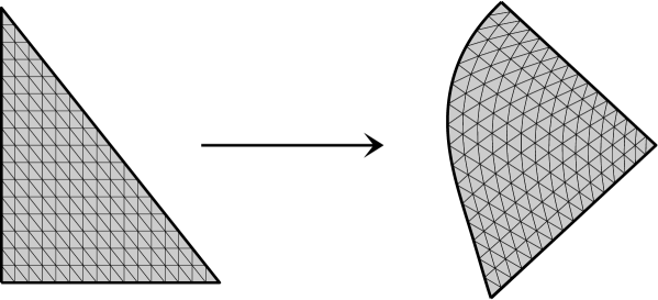
$\kappa_{k}$

Figure 2. Illustration of the diffeomorphim $\kappa_{k}:\triangle\to\tau_{0,k}$ and the construction of parametric finite elements.

The cell functions will be computed by the finite element method [6, 8]. To construct a triangulation which resolves the interface $\partial\omega$ exactly, we use parametric finite elements. To this end, we define a macro triangulation with the help of the parametric representation of $\partial\omega$ that consists of 28 curved elements based on the construction of Zenisek, cf. [42]. This macro triangulation yields a collection of smooth triangular patches $\{\tau_{0,k}\}$ and associated diffeomorphisms $\kappa_{k}:\triangle\to\tau_{0,k}$ (compare Figure 2) such that

(18) $$\overline{Y}=\bigcup_{k=1}^{28}\tau_{0,k},\quad\tau_{0,k}=\kappa_{k}(\triangle),\quad k=1,2,\ldots,28,$$

where $\triangle$ denotes the reference triangle in $\mathbb{R}^{2}$. The intersection $\tau_{0,k}\cap\tau_{0,k^{\prime}}$, $k\not=k^{\prime}$, of the patches $\tau_{0,k}$ and $\tau_{0,k^{\prime}}$ is either $\emptyset$, or a common edge or vertex. Moreover, the diffeomorphisms $\kappa_{k}$ and $\kappa_{k^{\prime}}$ coincide at a common edge except for orientation.

A mesh of level $\ell$ on $Y$ is induced by regular subdivisions of depth $\ell$ of the reference triangle into four sub-triangles. This generates the $4^{\ell}\cdot 28$ triangular elements $\{\tau_{\ell,k}\}$. An illustration of such a triangulation ($\ell=3$) is found in Figure 3. On the given triangulation, we employ continuous, piecewise linear finite elements to compute the cell functions, where the resulting system of linear equations is iteratively solved by the conjugate gradient method. Since the meshing procedure generates a nested sequence of finite element spaces, the Bramble-Pasciak-Xu (BPX) preconditioner [7] can be applied to precondition the iterative solution process. Notice that the triangulation resolves the interface and, thus, the convergence order of the approximate cell functions is optimal, i.e., second order in the mesh size $h$ with respect to the $L^{2}(Y)$-norm, cf. [23].

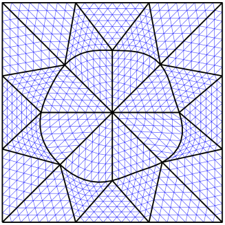
Figure 3. The macro triangulation consisting of 28 curved elements and the resulting mesh of the unit cell ${Y}$, which resolves the interface $\partial\omega$.

In the case of a perforated domain, we have to modify our finite element implementation correspondingly. In particular, the interior of $\omega$ is empty (hence, the macro triangulation consists of only 20 curved elements) and its boundary $\partial\omega$ serves as homogeneous Neumann boundary. These modifications of the implementation are straightforward, so that we skip the details.

For our numerical examples, we choose the expansion degree $N=32$ in (17), i.e., we consider 65 design parameters. Moreover, we use roughly $460\,000$ finite elements (which corresponds to the refinement level $\ell=7$ of the macro triangulation) for the domain discretization in order to solve the state equation for computing the shape functional and its gradient. The optimization procedure consists of gradient descent method, which is stopped when the $\ell^{2}$-norm of the discrete shape gradient is smaller than $\epsilon=10^{-5}$.

5.2. First example

For our first computations, we choose constant coefficient functions $\sigma_{1}\equiv 1$ and $\sigma_{2}\equiv 10$. The desired effective tensor in (6) is

$$\boldsymbol{B}_{1}=\begin{bmatrix}b_{1,1}&0\\ 0&1.4\end{bmatrix},$$

where $b_{1,1}$ varies from $1.1$ to $1.8$ with step size $0.1$. Starting with the circle of radius $1/4$ as initial guess, we obtain the optimal shapes found in Figure 4. Note that the desired effective tensor is achieved, i.e., the shape functional (6) is zero in the computed shapes. We especially see that the alignment of the computed shape reflects the anisotropy of the effective tensor.

$b_{1,1}=1.8$

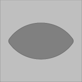
$b_{1,1}=1.7$

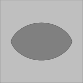
$b_{1,1}=1.6$

$b_{1,1}=1.5$

$b_{1,1}=1.4$

$b_{1,1}=1.3$

$b_{1,1}=1.2$

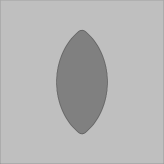
Figure 4. Optimal shapes for the desired effective tensor $\boldsymbol{B}_{1}$ in case of different values of $b_{1,1}$ when the circle of radius $1/4$ is used as initial guess.

5.3. Second example

We shall study the effect of the off-diagonal terms in the desired effective tensor. We thus consider

$$\boldsymbol{B}_{2}=\begin{bmatrix}1.4&b_{1,2}\\ b_{2,1}&1.4\end{bmatrix}$$

with $b_{1,2}=b_{2,1}$ chosen to be equal to $\pm 0.05$ and $\pm 0.1$. The results are found in Figure 5 in the order $-0.10$, $-0.05$, $0.05$, $0.10$ (from left to right) for the values of $b_{1,2}=b_{2,1}$. It is seen that the shape is oriented north-west in case of a negative sign and north-east in case of a positive sign. Notice that we obtain the circle found in Figure 4 in the situation $b_{1,2}=b_{2,1}=0$.

$b_{1,2}=-0.10$

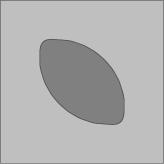
$b_{1,2}=-0.05$

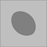
$b_{1,2}=0.05$

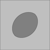
$b_{1,2}=0.10$

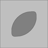
Figure 5. Optimal shapes for the desired effective tensor $\boldsymbol{B}_{2}$ in case of different values of $b_{1,2}=b_{2,1}$ when the circle of radius $1/4$ is used as initial guess.

5.4. Third example

In our next test, we shall show that the solution for $\omega$ is non-unique. To this end, we choose a randomly perturbed circle of radius $1/4$ as initial guess and try to construct a microstructure that has the (isotropic) effective tensor

(19) $$\boldsymbol{B}_{3}=\begin{bmatrix}1.4&0\\ 0&1.4\end{bmatrix}.$$

In Figure 6, we see the different shapes we get from the minimization of the shape functional (6), all of them resulting in the desired effective tensor $\boldsymbol{B}_{3}$. Notice that we obtain a circle if we would start with a circle as it can be seen in the fifth plot in Figure 4.

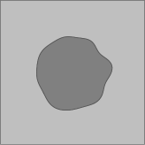
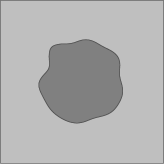
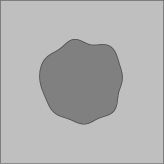
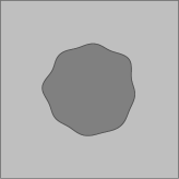
Figure 6. Optimal shapes for the desired effective tensor $\boldsymbol{B}_{3}$ when starting with a randomly perturbed circle as initial guess.

5.5. Fourth example

Likewise, we observe the same non-uniqueness if the desired effective tensor is anisotropic. Choosing

$$\boldsymbol{B}_{4}=\begin{bmatrix}1.6&0\\ 0&1.4\end{bmatrix}$$

and starting again by a randomly perturbed circle of radius $1/4$, we obtain the shapes found in Figure 7. All these shapes yield again the effective tensor $\boldsymbol{B}_{4}$. In case of starting with the circle of radius $1/4$, we get the shape seen in the third plot in Figure 4.

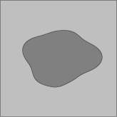
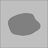
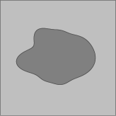
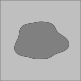
Figure 7. Optimal shapes for the desired effective tensor $\boldsymbol{B}_{4}$ when starting with a randomly perturbed circle as initial guess.

5.6. Fifth example

We shall also consider the situation that $\sigma_{1}$ and $\sigma_{2}$ are smooth functions. To this end, we consider $\sigma_{1}\equiv 1$ to be constant but

$$\sigma_{2}(x,y)=5\Bigg{(}\frac{11}{10}+\cos(2\pi x)+4\bigg{(}y-\frac{1}{2}\bigg{)}^{2}\Bigg{)}.$$

For the desired (isotropic) effective tensor $\boldsymbol{B}_{3}$ from (19) and the circle with radius $1/4$ as initial guess, we obtain the optimal shape found in the outermost left plot of Figure 8. If we randomly perturb the initial circle, then we obtain optimal shapes which are different, compare the other plots of Figure 8 for some results.

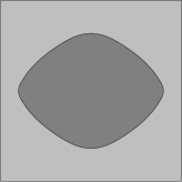
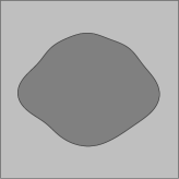
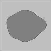
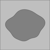
Figure 8. Different shapes which all generate the desired effective tensor $\boldsymbol{B}_{3}$ in case of a non-constant coefficient function $\sigma_{2}$.

5.7. Sixth example

We should finally have also a look at a perforated plate, which has been considered Section 4. We set $\sigma_{1}=1$ and choose

$$\boldsymbol{B}_{5}=\begin{bmatrix}0.8&0\\ 0&0.6\end{bmatrix}.$$

If we start the gradient method from the circle of radius $1/4$, we obtain the shape found in the outermost left plot of Figure 9. In case of starting with a randomly perturbed circle of radius $1/4$, we get the two shapes seen in the middle plots in Figure 9. Whereas, in the outermost right plot of Figure 9, we plotted the an ellipse which also leads to the desired effective tensor.

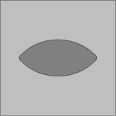
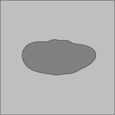
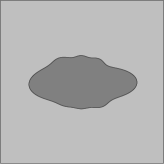
Figure 9. Different shapes which all generate the desired effective tensor $\boldsymbol{B}_{5}$ in case of a perforated domain.

6. Conclusion

In this article, shape sensitivity analysis of the effective tensor in case of composite materials and scaffold structures has been performed. In particular, we computed the shape gradient of the least square matching of a desired material property. In case of scaffold structures, we also provided the shape Hessian. This enables to apply the second order perturbation method to quantify uncertainties in the geometry of the hole. Numerical tests based on a finite element implementation in the two-dimensional setting have been performed for composite materials and for perforated domains. It has turned out that the computed optimal shapes depend on the initial guess, which means that the solution of the problem under consideration is in general not unique.

References

- [1] T. Adachi, Y. Osako, M. Tanakaa, M. Hojo, and S.J. Hollister. Framework for optimal design of porous scaffold microstructure by computational simulation of bone regeneration. Biomaterials 27 (2006) 3964–3972.
- [2] G. Allaire. Homogenization and two-scale convergence. SIAM J. Math. Anal. 23 (1992) 1482–1518.
- [3] G. Allaire, P. Geoffroy-Donders, and O. Pantz. Topology optimization of modulated and oriented periodic microstructures by the homogenization method. Preprint, hal-01734709v2 (2018).
- [4] G. Allaire, F. Jouve, and A.M. Toader. Structural optimization using sensitivity analysis and a level-set method. J. Comput. Phys. 194 (2004) 363–393.
- [5] A. Bensoussan, J.-L. Lions, and G. Papanicolaou. Asymptotic Analysis for Periodic Structures. North-Holland, Amsterdam, 1978.
- [6] D. Braess. Finite Elements. Theory, Fast Solvers, and Applications in Solid Mechanics. Cambridge University Press, Cambridge, 2001.
- [7] J. Bramble, J. Pasciak, and J. Xu. Parallel multilevel preconditioners. Mathematics of Computation 55 (1990) 1–22.
- [8] S. Brenner and L. Scott. The Mathematical Theory of Finite Element Methods. Springer, Berlin, 2008.
- [9] D. Cioranescu and J. Saint Jean Paulin. Homogenization of Reticulated Structures. Springer, New York, 1999.
- [10] L. Colabella, A.P. Cisilino, V. Fachinotti, and P. Kowalczyk. Multiscale design of elastic solids with biomimetic cancellous bone cellular microstructures. Struct. Multidiscip. Optim. 60 (2019) 639–661.
- [11] M. Dambrine, H. Harbrecht, and B. Puig. Computing quantities of interest for random domains with second order shape sensitivity analysis. ESAIM Math. Model. Numer. Anal. 49 (2015) 1285–1302.
- [12] M. Dambrine, and D. Kateb On the ersatz material approximation in level-set methods. ESAIM Control Optim. Calc. Var. 16 (2010) 618–634.
- [13] M. Dambrine, J. Sokolowski, and A. Zochowski. On stability analysis in shape optimization: critical shapes for Neumann problem. Control and Cybernetics 32 (2003) 503–528.
- [14] M. Delfour and J.-P. Zolesio. Shapes and Geometries. SIAM, Philadelphia, 2001.
- [15] A. Ferrer, J.C. Cante J.A. Hernández, and J. Oliver. Two-scale topology optimization in computational material design: An integrated approach. Int. J. Numer. Meth. Eng. 114 (2018) 232–254.
- [16] P. Geoffroy-Donders, G. Allaire, and O. Pantz. 3-d topology optimization of modulated and oriented periodic microstructures by the homogenization method. Preprint, hal-01939201 (2018).
- [17] J. Hadamard. Lectures on the Calculus of Variations. Gauthier–Villiars, Paris, 1910.
- [18] H. Harbrecht. On output functionals of boundary value problems on stochastic domains. Math. Meth. Appl. Sci. 33 (2010) 91–102.
- [19] S.J. Hollister, R.D. Maddox, and J.M. Taboas. Optimal design and fabrication of scaffolds to mimic tissue properties and satisfy biological constraints. Biomaterials 23 (2002) 4095–4103.
- [20] N. Hopkinson, R. Hague, P. Dickens. Rapid Manufacturing: An Industrial Revolution for the Digital Age, John Wiley & Sons, 2006.
- [21] D. Hübner, E. Rohan, V. Lukeš, and M. Stingl. Optimization of the porous material described by the Biot model. Int. J. Solids Struct. 156–157 (2019) 216–233.
- [22] R. Huiskes, H. Weinans, H.J. Grootenboer, M. Dalstra, B. Fudala, and T.J. Slooff. Adaptive bone-remodeling theory applied to prosthetic-design analysis. J. Biomechanics 20 (1987) 1135–1150.
- [23] J. Li, J.M. Melenk, B. Wohlmuth, and J. Zou. Optimal a priori estimates for higher order finite elements for elliptic interface problems. Appl. Numer. Math. 60 (2010) 19–37.
- [24] C.Y. Lin, N. Kikuchia, and S.J. Hollister. A novel method for biomaterial scaffold internal architecture design to match bone elastic properties with desired porosity. J. Biomechanics 37 (2004) 623–636.
- [25] D. Luo, Q. Rong, and Q. Chen. Finite-element design and optimization of a three-dimensional tetrahedral porous titanium scaffold for the reconstruction of mandibular defects. Med. Eng. Phys. 47 (2017) 176–183.
- [26] F. Murat and J. Simon. Étude de problèmes d’optimal design. In Optimization techniques, modeling and optimization in the service of man, edited by J. Céa, Lect. Notes Comput. Sci. 41, Springer, Berlin, 54–62 (1976).
- [27] G. Nika and A. Constantinescu. Design of multi-layer materials using inverse homogenization and a level set method. Comput. Methods Appl. Mech. Engrg. 346 (2019) 388–409.
- [28] G. Nguetseng. A general convergence result related to the theory of homogenization. SIAM J. Math. Anal. 20 (1989) 608–629.
- [29] D.K. Pattanayak, A. Fukuda, T. Matsushita, M. Takemoto, S. Fujibayashi, K. Sasaki, N. Nishida, T. Nakamura, and T. Kokubo. Bioactive Ti metal analogous to human cancellous bone. Fabrication by selective laser melting and chemical treatments. Acta Biomaterialia 7 (2011) 1398–1406.
- [30] O. Pironneau. Optimal Shape Design for Elliptic Systems. Springer, New York, 1984.
- [31] A. Reuss. Berechnung der Fließgrenze von Mischkristallen auf Grund der Plastizitätsbedingung für Einkristalle. Z. Angew. Math. Mech. 9 (1929) 49–58.
- [32] G. Rotta, T. Seramak, and K. Zasińska. Estimation of Young’s modulus of the porous titanium alloy with the use of FEM package. Adv. Mat. Sci. 15 (2015) 29–37
- [33] F. Schury, M. Stingl, and F. Wein. Efficient two-scale optimization of manufacturable graded structures. SIAM J. Sci. Comput. 34 (2012) B711–B733.
- [34] O. Sigmund. Tailoring materials with prescribed elastic properties. Mech. Mat. 20 (1995) 351–368.
- [35] J. Simon. Differentiation with respect to the domain in boundary value problems. Numer. Funct. Anal. Optim. 2 (1980) 649–687.
- [36] J. Sokolowski and J.-P. Zolesio. Introduction to Shape Optimization: Shape Sensitivity Analysis. Springer, 1992.
- [37] L. Tartar. The General Theory of Homogenization. A Personalized Introduction. Lecture Notes of the Unione Matematica Italiana, vol. 7, Springer, 2010.
- [38] W. Voigt. Über die Beziehung zwischen den beiden Elasticitätsconstanten isotroper Körper. Ann. Phys. 274 (1889) 573–587.
- [39] Y. Wang and Z. Kang. Concurrent two-scale topological design of multiple unit cells and structure using combined velocity field level set and density mode. Comput. Methods Appl. Mech. Engrg. 347 (2019) 340–364.
- [40] X. Wang, S. Xu, S. Zhou, W. Xu, M. Leary, P. Choong, M. Qian, M. Brandt, and Y.M. Xie. Topological design and additive manufacturing of porous metals for bone scaffolds and orthopaedic implants: A review. Biomaterials 83 (2016) 127–141.
- [41] M. Wormser, F. Wein, M. Stingl, and C. Körner. Design and additive manufacturing of 3D phononic band gap structures based on gradient based optimization. Materials 10 (2017) 1125.
- [42] A. Zenisek. Nonlinear Elliptic and Evolution Problems and Their Finite Element Approximation. Academic Press, San Diego, 1990.