Questaal: a package of electronic structure methods based on the linear muffin-tin orbital technique

Abstract

This paper summarises the theory and functionality behind Questaal, an open-source suite of codes for calculating the electronic structure and related properties of materials from first principles. The formalism of the linearised muffin-tin orbital (LMTO) method is revisited in detail and developed further by the introduction of short-ranged tight-binding basis functions for full-potential calculations. The LMTO method is presented in both Green’s function and wave function formulations for bulk and layered systems. The suite’s full-potential LMTO code uses a sophisticated basis and augmentation method that allows an efficient and precise solution to the band problem at different levels of theory, most importantly density functional theory, LDA$+U$, quasi-particle self-consistent GW and combinations of these with dynamical mean field theory. This paper details the technical and theoretical bases of these methods, their implementation in Questaal, and provides an overview of the code’s design and capabilities.

PROGRAM SUMMARY

Program Title: Questaal
Licensing provisions: GNU General Public License, version 3
Programming language: Fortran, C, Python, Shell
Nature of problem: Highly accurate ab initio calculation of the electronic structure of periodic solids and of the resulting physical, spectroscopic and magnetic properties for diverse material classes with different strengths and kinds of electronic correlation.
Solution method: The many electron problem is considered at different levels of theory: density functional theory, many body perturbation theory in the GW approximation with different degrees of self consistency (notably quasiparticle self-consistent GW) and dynamical mean field theory. The solution to the single-particle band problem is achieved in the framework of an extension to the linear muffin-tin orbital (LMTO) technique including a highly precise and efficient full-potential implementation. An advanced fully-relativistic, non-collinear implementation based on the atomic sphere approximation is used for calculating transport and magnetic properties.

1 Introduction

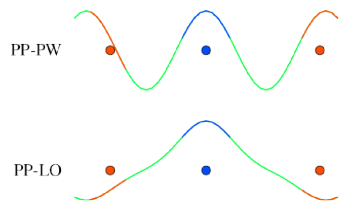
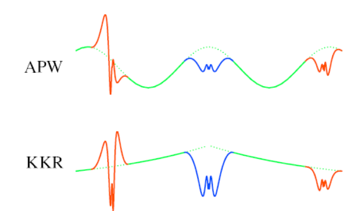
Figure 1: $2{\times}2$ rubric for main classifications of basis set. Nuclei are shown as dots. The all-electron methods APW and KKR on the right substitute (augment) the envelope function (green) with numerical solutions of partial waves inside augmentation spheres (blue and red). Parts inside augmentation spheres are called “partial waves.” The two figures on the left use a pseudopotential allowing their envelope functions to be smooth, with no augmentation needed. A pseudopotential’s radius corresponds to a characteristic augmentation radius. The top two figures use plane waves for envelope functions; the bottom two use atom-centred local basis sets. We denote localised basis sets as “KKR”, for the Korringa-Kohn-Rostocker method [1] as it plays a central role in this work; but there are other kinds, for example the Gaussian orbitals widely favoured among quantum chemists.

Different implementations of DFT are distinguished mainly by their basis set, which forms the core of any electronic structure method, and how they orthogonalise themselves to the core levels. Using these classifications most methods adopt one of four possible combinations shown in Fig. 1. In the vast majority of cases, basis sets consist of either atom-centred spatially localised functions (lower panel of Fig. 1), or plane waves (PW) (upper). As for treatment of the core, it is very common to substitute an effective repulsive (pseudo)potential to simulate its effect, an idea initially formulated by Conyers Herring [2]. Pseudopotentials make it possible to avoid orthogonalisation to the core, which allows the (pseudo)wave functions to be nodeless and smooth. For methods applied to condensed matter, the primary alternative method, formulated by Slater in 1937 [3], keeps all the electrons. Space is partitioned into non-overlapping spheres centred at each nucleus, with the interstitial region making up the rest. The basis functions are defined by plane waves in the interstitial, which are replaced (“augmented”) by numerical solutions of the Schrödinger equations (partial waves) inside the augmentation spheres. The two solutions must be joined smoothly and differentiably on the augmentation sphere boundary (minimum conditions for a non-singular potential). Slater made a simplification: he approximated the potential inside the augmentation spheres with its spherical average, and also the interstitial potential with a constant. This is called the Muffin Tin (MT) approximation; see Fig. 2.

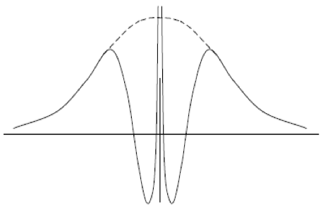
Figure 2: Left: basis function in the vicinity of a nucleus, showing orthogonalisation to core states (solid line), and corresponding basis function in a pseudopotential (dashed line). Right: a muffin-tin potential: the potential is flat in the interstitial region between sites, and spherically symmetric in a volume around each site. Blue depicts an augmentation radius $s_{R}$ around a sphere centred at some nuclear position ${{\mathbf{R}}}$ where the interstitial and augmented regions join.

Solutions to spherical potentials are separable into radial and angular parts, $\phi_{\ell}(\varepsilon,r)Y_{L}(\hat{{{\mathbf{r}}}})$. The $\phi_{\ell}$ are called partial waves and $Y_{L}$ are the spherical harmonics. Here and elsewhere, angular momentum labelled by an upper case letter refers to both the $\ell$ and $m$ parts. A lower case symbol refers to the orbital index only ($\ell$ is the orbital part of $L{=}(\ell,m)$). The $\phi_{\ell}$ are readily found by numerical integration of a one-dimensional wave equation (Sec. 2), which can be efficiently accomplished.

An immense amount of work has followed the original ideas of Herring and Slater. The Questaal package is an all-electron implementation in the Slater tradition, so we will not further discuss the vast literature behind the construction of a pseudopotential, except to note there is a close connection between pseudopotentials and the energy linearisation procedure to be described below. Blöchl’s immensely popular Projector Augmented-Wave method [4] makes a construction intermediate between pseudopotentials and APWs. Questaal uses atom-centred envelope functions instead of plane waves (Sec. 3), and an augmentation scheme that resembles the PAW method but can be converged to an exact solution for the reference potential, as Slater’s original method did. The spherical approximation is still almost universally used to construct the basis set, and thanks to the variational principle, errors are second order in the nonspherical part of the potential. The nonspherical part is generally quite small, and this is widely thought to be a very good approximation, and the Questaal codes adopt it.

For a MT potential ($V_{MT}$ taken to be 0 for simplicity), the Schrödinger equation for energy $\varepsilon$ has locally analytical solutions: in the interstitial the solution can expressed as a plane wave $e^{i\,\mathbf{k}\cdot{{\mathbf{r}}}}$, with $\varepsilon{=}\hbar^{2}k^{2}/2m$. (We will use atomic Rydberg units throughout, $\hbar{=}2{m}{=}e^{2}/2{=}1$). In spherical coordinates envelope functions can be Hankel functions $H_{L}(E,{{\mathbf{r}}}){=}h_{\ell}(kr)Y_{L}(\hat{{{\mathbf{r}}}})$ or Bessel functions $j_{\ell}(kr)Y_{L}(\hat{{{\mathbf{r}}}})$, except that Bessel functions are excluded as envelope functions because they are not bounded in space. Inside the augmentation spheres, solutions consist of some linear combination of the $\phi_{\ell}$.

The all-electron basis sets “APW” (augmented plane wave) and “KKR” [1] are both instances of augmented-wave methods: both generate arbitrarily accurate solutions for a muffin-tin potential. They differ in their choice of envelope functions (plane waves or Hankel functions), but they are similar in that they join onto solutions of partial waves in augmentation spheres. Both basis sets are energy-dependent, which makes them very complicated and their solution messy and slow. This difficulty was solved by O.K. Andersen in 1975 [5]. His seminal work paved the way for modern “linear” replacements for APW and KKR, the LAPW and Linear Muffin Tin Orbitals (LMTO) method. By making a linear approximation to the energy dependence of the partial waves inside the augmentation spheres (Sec. 2.4), the basis set can be made energy-independent and the eigenfunctions and eigenvalues of the effective one-particle equation obtained with standard diagonalisation techniques. LAPW, with local orbitals added to widen the energy window over which the linear approximation is valid (Sec. 3.7.3) is widely viewed to be the industry gold standard for accuracy. Several well known codes exist:WIEN2K (http://susi.theochem.tuwien.ac.at) and its descendants such as the Exciting code (http://exciting-code.org) and FLEUR (http://www.flapw.de). A recent study [6] established that these codes all generate similar results when carefully converged. Questaal’s main DFT code is a generalisation of the LMTO method (Sec. 3), using the more flexible smooth Hankel functions (Sec. 3.1) instead of standard Hankels for the envelope functions. Accuracy of the smooth-Hankel basis is also high (Sec. 3.13), and though not quite reaching the standard of the LAPW methods, it is vastly more efficient. If needed, Questaal can add APW’s to the basis to converge it to the LAPW standard (Sec. 3.10).

1.1 Questaal’s History

Questaal has enjoyed a long and illustrious history, originating in O.K. Andersen’s group in the 1980’s as the standard “Stuttgart” code. It has undergone many subsequent evolutions, e.g. an early all-electron full-potential code [7], which was used in one of the first ab initio calculations of the electron-phonon interaction for superconductivity [8], an efficient molecules code [9] which was employed in the first ab initio description of instanton dynamics [10], one of the first noncollinear magnetic codes and the first ab initio description of spin dynamics [11], first implementation of exact exchange and exact exchange+correlation [12], one of the first all-electron GW implementations [13], and early density-functional implementations of non-equilibrium Green’s functions for Landauer-Buttiker transport [14]. In 2001 Aryasetiawan’s GW was extended to a full-potential framework to become the first all-electron GW code [15]. Soon after the concept of quasiparticle self-consistency was developed [16], which has dramatically improved the quality of GW. Its most recent extension is to combine QSGW with DMFT. It and the code of Kutepov et al. [17] are the first implementations of QSGW+dynamical mean field theory (DMFT); and to the best of our knowledge it has the only implementation of response functions (spin, charge, superconducting) within QSGW+DMFT.

1.2 Main Features of the Questaal Package

Ideally a basis set is complete, minimal, and short ranged. We will use the term compact to mean the extent to which a basis can satisfy all these properties: the faster a basis can yield converged results for a given rank of Hamiltonian, the more compact it is. It is very difficult to satisfy all these properties at once. KKR is by construction complete and minimal for a “muffin-tin” potential, but it is not short-ranged. In 1984 it was shown (by Andersen once again! [18]) how to take special linear combinations of muffin-tin orbitals (“screening transformation”) to make them short ranged. Andersen’s screening transformation was derived for LMTOs, in conjunction with his classic Atomic Spheres Approximation, (ASA, Sec. 2.7), and screening has subsequently been adopted in KKR methods also. The original Questaal codes were designed around the ASA, and we develop it first in Sec. 2.5. Its main code no longer makes the ASA approximation, and generalises the LMTOs to more flexible functions; that method is developed in Sec. 3. These functions are nevertheless long-ranged and cannot take advantage of very desirable properties of short-ranged basis sets. Very recently we have adapted Andersen’s screening transformation to the flexible basis of full-potential method (Sec. 2.9). Screening provides a framework for the next-generation basis of “Jigsaw Puzzle Orbitals” (JPOs) that will be a nearly optimal realisations of the three key properties mentioned above.

Most implementations of GW are based on plane waves (PWs), in part to ensure completeness, but also because implementation is greatly facilitated by the fact that the product of two plane waves is analytic. GW has also been implemented recently in tight-binding forms using e.g., a numerical basis [19], or a Gaussian basis [20]. None of these basis sets is very compact. The FHI AIMS code can be reasonably well converged, but only at the expense of a large number of orbitals. Gaussian basis sets are notorious for becoming over-complete before they become complete. Questaal’s JPO basis—still under development—should bring into a single framework the key advantages of PW and localised basis sets.

Questaal implements:

1. density-functional theory (DFT) based on common LDA and GGA exchange-correlation functionals (other LDA or GGA, but not meta-GGA, varients are available via libxc[21]). There is a standard full-potential DFT code, lmf (Sec. 3), and also three codes (lm, lmgf, lmpg) that implement DFT in the classical Atomic Spheres Approximation [5, 18], presented in Sec. 2.7. The latter use the screened, tight-binding form (Sec. 2.10). lm, a descendant of Andersen’s standard ASA package (Stuttgart code), is an approximate, fast form of lmf, useful mainly for close-packed magnetic metals; lmgf (Sec. 2.12) is a Green’s function implementation closely related to the KKR Green’s function, parameterised so that it can be linearised. Sec. 2.13 shows how this is accomplished, resulting in an efficient, energy-independent Hamiltonian lm uses. lmgf has two useful extensions: the coherent potential approximation (CPA, Sec. 2.18) and the ability to compute magnetic exchange interactions. lmpg (Sec. 2.14) is a principal layer Green’s function technique similar to lmgf but designed for layer geometries (periodic boundary conditions in two dimensions). lmgf is particularly useful for Landauer-Buttiker transport [22, 23, 24, 25], and it includes a nonequilibrium Keldysh technique [14].

2. density functional theory with local Hubbard corrections (LDA+U) with various kinds of double-counting correction (Sec. 3.8).

3. the GW approximation based on DFT. Questaal’s GW package is separate from the DFT code; there is an interface (lmfgwd) that supplies DFT eigenfunctions and eigenvalues to it. It was originally formulated by Aryasetiawan in the ASA [26], derived from the Stuttgart ASA code; and it was the first all-electron GW implementation. Kotani and van Schilfgaarde extended it to a full-potential framework in 2002 [15]. A shell script lmgw runs the GW part and manages links between it and lmf;

4. the Quasiparticle Self-Consistent GW (QSGW) approximation, first formulated by Faleev, Kotani and van Schilfgaarde [16]. Questaal’s QSGW is a descendent of Kotani’s original code, which with some modest modifications can be found at https://github.com/tkotani/ecalj/. QSGW also works synchronously with lmf, yielding either a static QSGW self-energy $\Sigma_{0}$ which lmf reads as an effective external potential added to the Hamiltonian, or a dynamical self-energy (diagonal part) which a post-processing code lmfgws, uses to construct properties of an interacting Green’s function, such as the spectral function. See Sec. 4;

5. extensions to Dynamical Mean Field Theory using a bath based on either DFT or QSGW. Questaal does not have its own implementation of DMFT, but has interfaces to Haule’s CTQMC solver [27], and to the TRIQS library [28]. See Sec. 5;

6. an empirical tight-binding model (tbe). The interested reader is referred to Refs [29, 30] and the Questaal web site; and

7. a large variety of other codes and special-purpose editors to supply input the electronic structure methods, or to process the output.

1.3 Outline of the Paper

The aim of the paper is to provide a consistent presentation of the key expressions and ideas of the LMTO method, and aspects of electronic structure theory as they are implemented in the different codes in the Questaal suite. Necessarily this presentation is rather lengthy; the paper is organised as follows. Section 2 describes the LMTO basis, assuming the muffin-tin and atomic sphere descriptions of the potential. Together with tail cancellation and linearisation this comprises therefore a derivation of the traditional (“second generation”) LMTO method. The transformation to a short range tight-binding-like basis, and to other representations is described. The formulation of the crystal Green’s function in terms of the LMTO potential parameters is derived, allowing the use of coherent potential approximation alloy theory. Non-collinear magnetism and fully-relativistic LMTO techniques are presented. Section 3 describes the full-potential code: its basis, augmentation method, core treatment and other technical aspects are described in detail. The LDA$+U$ method, relativistic effects, combined LMTO+APW, and numerical precision are also discussed. Section 4 describes the GW method: the importance of self-consistency, the nature of QSGW in particular and its successes and limitations. Section 5 describes Questaal’s interface to different DMFT solvers; section 6 discusses calculation of spin and charge susceptibilities. Our perspective on realising a high fidelity solution to the many-body problem for solids is described in section 7. Finally, software aspects of the Questaal project are outlined in section 8. Several appendices are provided with a number of useful and important relations for the LMTO methodology.

2 The Muffin-Tin Potential and the Atomic Spheres Approximation

As noted earlier, the KKR method solves the Schrödinger equation in a MT potential to arbitrarily high accuracy. We develop this method first, and show how the LMTO method is related to it. In Sec. 3.1 we show how the basis in lmf is related to LMTOs. The original KKR basis set consists of spherical Hankel (Neumann) functions $H_{RL}(E,{{\mathbf{r}}})=h_{R\ell}(kr)Y_{L}(\hat{{{\mathbf{r}}}})$ as envelope functions with $k^{2}=E$, augmented by linear combinations of partial waves $\phi_{R\ell}(\varepsilon,r)Y_{RL}(\hat{{{\mathbf{r}}}})$ inside augmentation spheres (Fig. 3). (See the Appendix for definitions and the meaning of subscripts $R$ and $L$.) The envelope must be joined continuously and differentiably onto augmentation parts, since the kinetic energy cannot be singular. Note that for large $\ell$, $\phi_{R\ell}\rightarrow\text{const}{\times}r^{\ell}$. This is because the angular part of the kinetic energy becomes dominant for large $\ell$.

Figure 3: Schematic of muffin-tin potential (black) and a solution (red) in a three-atom chain.

2.1 One-centre Expansion of Hankel Functions

An envelope function $H_{L}(E,{{\mathbf{r}}})$ has a “head” centred at the origin where it is singular and tails at sites around the origin. In addition to the head, tails must be augmented by linear combinations of $\phi_{\ell}(\varepsilon,r)$ centred there, which require $H_{L}$ be expanded in functions centred at another site. If the remote site is at ${{\mathbf{R}}}$ relative to the head, the one-centre expansion can be expressed as a linear combination of Bessel functions

$$H_{L}(E,{{\mathbf{r}}})=\sum_{M}S_{ML}(E,{{\mathbf{R}}})J_{M}(E,\mathbf{r-{{\mathbf{R}}}})$$ (1)

This follows from the fact that both sides satisfy the same second order differential equation $(\nabla^{2}+E)=0$. The two functions centred at the origin satisfying this equation are the Hankel and Bessel functions. Hankel functions have a pole at $r=0$, whereas Bessel functions are regular there, so this relation must be true for all $r<|{{\mathbf{R}}}|$. The larger the value of $r$, the slower the convergence with $M$.

Expressions for the expansion coefficients $S$ can be found in various textbooks; they of course depend on how $H$ and $J$ are defined. Our standard definition is

$$S_{MK}(E,{\bf R})=$$

$$4\pi\sum_{L}C_{KLM}(-1)^{k}(-E)^{(k+m-\ell)/2}H_{L}(E,{\bf R})$$ (2)

The $C_{KLM}$ are Gaunt coefficients (Eq. (A.8)).

To deal with solids with many sites, we write the one-centre expansion using subscript $R$ to denote a nucleus and ${{\mathbf{r}}}$ relative to the nuclear coordinate:

$$H_{RL}(E,{{\mathbf{r}}})=\sum_{M}S_{R^{\prime}M,RL}(E)J_{R^{\prime}M}(E,{{\mathbf{r}}})$$ (3)

Envelope functions then have two $\ell$ cutoffs: $\ell_{b}$ for the head at $R$, and $\ell_{a}$ for the one-centre expansion at $R^{\prime}$. These need not be the same: $\ell_{b}$ determines the rank of the Hamiltonian, while $\ell_{a}$ is a cutoff beyond which $\phi_{R^{\prime}\ell}\times\phi_{R^{\prime}\ell^{\prime}}$ is well approximated by $\text{const}{\times}r^{\ell+\ell^{\prime}}$. A reasonable rule of thumb for reasonably well converged calculations is to take $\ell_{b}$ one number larger than the highest $\ell$ character in the valence bands. Thus $\ell_{b}=2$ is reasonable for $sp$ elements, $\ell_{b}=3$ for transition metal elements, $\ell_{b}=4$ for $f$ shell elements. In the ASA, reasonable results can be obtained for $\ell_{b}=2$ for transition metal elements, and $\ell_{b}=3$ for $f$ shell elements. As for $\ell_{a}$, traditional forms of augmentation usually require $\ell_{a}=2\ell_{b}$ for comparable convergence: lmf does it in a unique way that converges much faster than the traditional form and it is usually enough to take $\ell_{a}=\ell_{b}+1$ [31] (Sec. 3.6).

2.2 Partial Waves in the MT Spheres

Partial waves in a sphere of radius $s$ about a nucleus must be solved in the four coordinates, ${{\mathbf{r}}}$ and energy $\varepsilon$. Provided ${{\mathbf{r}}}$ is not too large, $v(\bf{r})$ is approximately spherical, $v({{\mathbf{r}}}){\approx}v(r)$; Even if the potential is not spherical, it is assumed to be for construction of the basis set, as noted earlier. Solutions for a spherical potential are partial waves $\phi_{\ell}(\varepsilon,r)Y_{L}(\hat{{{\mathbf{r}}}})$, where $Y_{L}$ are the spherical harmonics. Usually Questaal uses real harmonics $\text{Y}_{L}(\hat{{{\mathbf{r}}}})$ instead (see Appendix for definitions).

$\phi_{\ell}(\varepsilon,r)$ satisfies Schrödinger’s equation

$$(-{\nabla^{2}}+v(r)-{\varepsilon})\phi_{\ell}({\varepsilon},r)=0$$ (4)

We are free to choose the normalisation of $\phi$ and use

$$\int_{0}^{s}\phi^{2}(\varepsilon,r)r^{2}dr=1$$ (5)

One way to think about solutions of Schrödinger’s equation is to imagine each nucleus, with some $v_{R}(r)$ around it, as a scatterer to waves incident on it. Scattering causes shifts in the phase of the outgoing wave. The condition that all the sites scatter coherently, which allows them to sustain each other without any incident wave, gives a solution to Schrödinger’s equation. This condition is explicit in the KKR method, and forms the basis for it. Imagine a “muffin -tin” potential—flat in the interstitial but holes carved out around each nucleus of radius $s$. The phase shift from a scatterer at R is a property of the shape of $\phi_{R\ell}$ at its MT boundary, $\phi_{R\ell}(\varepsilon,s)$. Complete information about the scattering properties of the sphere, if $v({{\mathbf{r}}}){=}v(r)$, can be parameterised in terms of $\phi_{R\ell}(\varepsilon,s)$ and its slope, as we will see.

For a small change in energy of the incident wave, there can be a strong change in the phase shift. In the region near an eigenstate of the free atom the energy dependence is much stronger for the partial wave than it is for the incident waves striking it, so electronic structure methods focus on the scattering properties of the partial waves $\phi_{\ell}$. This information is typically expressed through the logarithmic derivative function

$$D_{\ell}(\varepsilon)\equiv D\{\phi_{\ell}(\varepsilon)\}=\left({\frac{r}{\phi_{\ell}(\varepsilon,r)}}{\frac{d\phi_{\ell}(\varepsilon,r)}{dr}}\right)_{s}$$ (6)

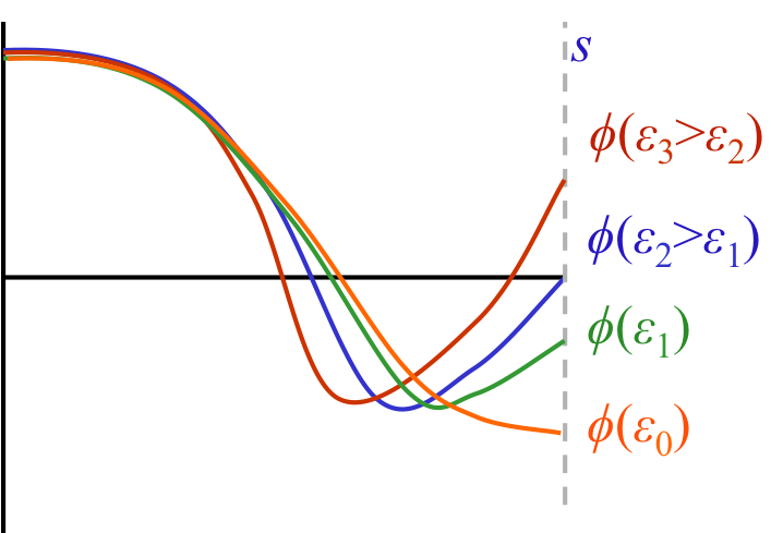
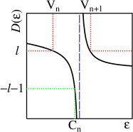
Figure 4: Variation of $\phi_{\ell}(\varepsilon,r)$ with $\varepsilon$ for an $s$ orbital.

Consider the change in $\phi_{\ell}(\varepsilon,r)$ with $\varepsilon$ for a given $v(r)$. As $\varepsilon$ increases $\phi_{\ell}(\varepsilon,r)$ acquires more curvature (Fig. 4). In the interval between $\varepsilon{=}\varepsilon_{0}$ where $\phi^{\prime}_{\ell}(\varepsilon_{0},s){=}0$ so that $D_{\ell}=0$, and $\varepsilon_{2}$ where $\phi_{\ell}(\varepsilon_{2},s){=}0$, $\phi^{\prime}_{\ell}(\varepsilon,s)$ is positive. $D_{\ell}$ thus decreases monotonically, with $D_{\ell}\to{-}\infty$ as $\varepsilon{\rightarrow}\varepsilon_{2}$. At some $\varepsilon_{1}$ in this region $D_{\ell}{=}-\ell-1$, which is the logarithmic derivative of a Hankel function of energy 0. $\varepsilon_{1}$ is called the “band centre” $C_{\ell}$ for reasons to be made clear in Sec. 2.5: it is close to an atomic level and in tight-binding theory would correspond to an on-site matrix element. Increasing from $\varepsilon_{2}$, $D_{\ell}$ decreases monotonically from ${+}\infty$ as shown in Fig. 4, reaching 0 once more, passing through some $\varepsilon_{3}$ where $D_{\ell}{=}+\ell$. This is the logarithmic derivative of a Bessel function of energy 0, and is traditionally called $V_{\ell}$.

Thus $D_{\ell}$ is a monotonically decreasing cotangent-like function of $\varepsilon$, with a series of poles. At each pole $\phi_{\ell}(\varepsilon,r)$ acquires an additional node, incrementing the principal quantum number $n$. Between poles $n$ is fixed and there are parameters $C_{\ell}$ and $V_{\ell}$ for each $n$. The linear method approximates $D_{\ell}$ with a simple pole structure, which is accurate over a certain energy window. Similarly pseudopotentials are constructed by requiring the pesudofunction to match $D_{\ell}$ of the free atom, in a certain energy window.

For principal quantum number $n$, $\phi_{\ell}$ has $n{-}\ell{-}1$ nodes and may vary rapidly to be orthogonal to deeper nodes. This poses no difficulty: we use a shifted logarithmic radial mesh, with point $i$ given by

$$r_{i}=b\{e^{a(i-1)}-1\}$$

Typically a few hundred points are needed for accurate integration. Core and valence waves use the same mesh.

2.3 Energy Derivative of D

Consider the matrix element integrated over a sphere of radius $s$:

$$0=\left\langle{\phi_{\ell}(\varepsilon_{\nu})}\right|-\nabla^{2}+v-\varepsilon\left|{\phi_{\ell}(\varepsilon)}\right\rangle$$

$\varepsilon_{\nu}$ is some fixed energy. Taking into account the boundary condition at $s$, we obtain

$$\left\langle{\phi_{\ell}(\varepsilon)}\right|\varepsilon-\varepsilon_{\nu}\left|{\phi_{\ell}(\varepsilon_{\nu})}\right\rangle=\\ -[D_{\ell}(\varepsilon)-D_{\ell}\left({\varepsilon_{\nu}}\right)]s\phi_{\ell}(\varepsilon_{\nu},s)\phi_{\ell}(\varepsilon,s)$$

from Green’s second identity. From this we obtain the energy derivative of $D_{\ell}$ as [5]

$$\dot{D}_{\ell}(\varepsilon)\equiv\mathop{\lim}\limits_{\varepsilon\to\varepsilon_{\nu}}\frac{{D_{\ell}(\varepsilon)-D_{\ell}\left({\varepsilon_{\nu}}\right)}}{{\varepsilon-\varepsilon_{\nu}}}=\frac{{-1}}{{s\phi_{\ell}^{2}(\varepsilon,s)}}$$ (7)

2.4 Linearisation of Energy Dependence in the Partial Waves

An effective way to solve Schrödinger’s equation is to linearise the energy-dependence of the partial waves $\phi_{\ell}(\varepsilon,r)$, as

$$\phi_{\ell}(\varepsilon,r)\approx\phi_{\ell}(\varepsilon_{\nu},r)+(\varepsilon-\varepsilon_{\nu})\dot{\phi}_{\ell}(\varepsilon_{\nu},r)$$ (8)

This was Andersen’s most important contribution to electronic structure theory [5]: it had a dramatic impact on the entire field. We will make extensive use of the linear approximation here.

In the linear approximation, four parameters ($\phi(s)$, $\dot{\phi}(s)$, and their logarithmic derivatives) completely characterise the scattering properties of a sphere with $v=v(r)$. Only three of them turn out to be independent. To see this, obtain an equation for $\dot{\phi}$ by differentiating Eq. (4) w.r.t. $\varepsilon$:

$$(-{\nabla^{2}}+v-{\varepsilon}){\dot{\phi}({\varepsilon},r)}=\phi({\varepsilon},r)$$ (9)

With the normalisation Eq. (5), $\phi$ and $\dot{\phi}$ are orthogonal

$$\langle\phi(\varepsilon_{\nu})\dot{\phi}(\varepsilon_{\nu})\rangle=0$$ (10)

Using the normalisation Eq. (5), we can establish the following relation between $\phi({\varepsilon_{\nu}},s)$, $\dot{\phi}({\varepsilon_{\nu}},s)$, $D\{\phi\}$ and $D\{\dot{\phi}\}$:

$$1 =\langle{{{[\phi({\varepsilon_{\nu}})]}^{2}}}\rangle=\langle{\phi({\varepsilon_{\nu}})|-{\nabla^{2}}+v-{\varepsilon_{\nu}}|\dot{\phi}({\varepsilon_{\nu}})}\rangle$$

$$=\langle{\dot{\phi}({\varepsilon_{\nu}})|-{\nabla^{2}}+v-{\varepsilon_{\nu}}|\phi({\varepsilon_{\nu}})}\rangle+W\{\phi,\dot{\phi}\}$$

$$=W\{\phi(s),\dot{\phi}(s)\}$$

$$=[D\{\phi({\varepsilon_{\nu}})\}-D\{\dot{\phi}({\varepsilon_{\nu}})\}]s\phi({\varepsilon_{\nu}},s)\dot{\phi}({\varepsilon_{\nu}},s)$$ (11)

The third line follows from Eq. (4), and the second from Green’s second identity which adds a surface term when $\phi$ and $\dot{\phi}$ are interchanged. The Wronskian $W\{a,b\}$ is defined as

$$W\{a(s),b(s)\} \equiv s^{2}\left[a(s)b^{\prime}(s)-a^{\prime}(s)b(s)\right]$$

$$=sa(s)b(s)\left[D\{b\}-D\{a\}\right]$$ (12)

for a pair of functions $a(r)$ and $b(r)$ evaluated at point $s$.

2.5 The Traditional LMTO Method

For historical reasons Anderson constructed the original LMTO formalism with non-standard definitions for the Hankel and Bessel functions. We follow those definitions in order to be consistent with the historical literature. In this paper they are named $\hat{H}_{\ell}$ and $\hat{J}_{\ell}$ and are defined in Appendix B. Here we follow Andersen’s development only in the context of $E{\leq}0$, with $\kappa^{2}{=}-E$. Note that $E$ can be chosen freely and need not be connected to the eigenvalue $\varepsilon$. But for exact solutions in a MT potential, the energy of $\hat{H}_{L}(E,{{\mathbf{r}}})$ and $\hat{J}_{\ell}(E,{{\mathbf{r}}})$ must be chosen so $E{=}\varepsilon{-}v_{\text{MTZ}}$.

LMTO and KKR basis sets solve Schrödinger’s equation in a muffin-tin potential, which in the interstitial reduces to the Helmholtz equation, and have linear combinations of Hankel functions as solutions that satisfy appropriate boundary conditions. We defer treatment of the boundary conditions to the next section and continue the analysis of partial waves for a single scattering centre for now.

As noted, the scattering properties depend much more strongly on the partial waves than the energy dependence of the envelopes. In keeping with the traditional LMTO method, we assume that the kinetic energy of the envelopes vanishes (the energy is taken to be close to the MT potential), then Schrödinger’s equation reduces further to Laplace’s equation, whose solutions are Hankel and Bessel functions $\hat{H}_{\ell}$ and $\hat{J}_{\ell}$ at $E{=}0$, which we denote as $\hat{H}_{\ell}({{\mathbf{r}}})$ and $\hat{J}_{\ell}({{\mathbf{r}}})$. In close-packed solids there is reasonable justification for this choice: the spacing between spheres is much smaller than the wavelength of a low-energy solution to the wave equation (one not too far from the Fermi level). $\hat{H}_{\ell}({{\mathbf{r}}})$ and $\hat{J}_{\ell}({{\mathbf{r}}})$ are proportional to $r^{-\ell-1}$ and $r^{\ell}$ respectively (see Appendix) and so $\phi_{\ell}$ can be continued into the interstitial in the vicinity of $s$

$$\phi_{\ell}(\varepsilon,r{\sim}s)=\phi_{\ell}\left({\varepsilon,s}\right)\frac{{\ell+1+D\{\varepsilon\}}}{{2\ell+1}}\left({\frac{r}{s}}\right)^{\ell}\\ +\phi_{\ell}\left({\varepsilon,s}\right)\frac{{\ell-D\{\varepsilon\}}}{{2\ell+1}}\left({\frac{s}{r}}\right)^{\ell+1}$$ (13)

The first term is proportional to $\hat{J}_{\ell}(r)$, the second to $\hat{H}_{\ell}(r)$. In the remainder of this section we will develop expressions for the general $\kappa$ case, showing also the $\kappa{\to}0$ limit, and finally focus on constructing Hamiltonians and Green’s functions with $\kappa{=}0$.

2.6 Energy-Dependent Muffin-Tin Orbitals

Eq. (13) is not yet a suitable basis because it diverges as $r{\to}{\infty}$ because of the $J_{\ell}$ term. However, we can construct a family of “muffin-tin” orbitals that are continuous and differentiable

$$\chi_{RL}(\varepsilon,E,{{{\mathbf{r}}}})={Y_{L}(\hat{{{\mathbf{r}}}}_{R})}\times$$

$$\begin{cases}{N_{R\ell}\left({\varepsilon}\right){\phi_{R\ell}}\left({\varepsilon,r_{R}}\right)+P_{R\ell}\left({\varepsilon}\right){\hat{J}_{\ell}}(E,r_{R})}&{{r_{R}}<{s_{R}}}\\ {{\hat{H}_{\ell}}(E,r_{R})}&{{r_{R}}>{s_{R}}}\end{cases}$$ (14)

and that do not diverge for large $r_{R}$. $N_{R\ell}$ and $P_{R\ell}$ are coefficients fixed by requiring that the value and slope are continuous at $s_{R}$. Thus for $r{<}s$, $\chi_{RL}(\varepsilon,E,{{{\mathbf{r}}}})$ consists of a linear combination of $\phi_{R\ell}(r)$ and $\hat{J}_{R\ell}(E,r)$ that matches smoothly and differentiably onto $\hat{H}_{R\ell}(E,r)$. Apart from the “contaminating” $\hat{J}_{R\ell}$ term, $\chi_{RL}$ is a solution for a single MT potential at sphere $R$. It vanishes at $\varepsilon$ corresponding to the eigenvalue of the MT “atom,” which occurs at $\varepsilon{=}C_{\ell}$. (Taking $E{=}0$, $\varepsilon{=}C_{\ell}$ when $D_{\ell}{=}-\ell-1$; see Eq. (13).) In a lattice ${\hat{H}_{\ell}}$ must also be augmented at all $R^{\prime}{\neq}R$. To form an eigenstate, the contaminating term must be cancelled out by tails from $\chi_{R^{\prime}L^{\prime}}$ centred elsewhere. Since any $\hat{H}_{R^{\prime}L^{\prime}}(E,r)$ can be expanded as linear combinations of $\hat{J}_{RL}(E,r)$, Eq. (3), it is easy to anticipate how the “tail cancellation condition,” which forms the basis of the KKR method (2.6.1), comes about.

The $P_{\ell}$ are called “potential functions” and play a central role in constructing eigenfunctions. Expressions for $P_{\ell}$ and $N_{\ell}$ are developed in Sec. 2.8. Combined with the linearisation of the partial waves, (Sec. 2.4), information about $P$ can be encapsulated in a small number of parameters; see Sec. 2.8.1.

Note the similarity between the $\chi_{RL}$ and the partial waves. There is a difference in normalisation, but more importantly the term proportional to $\hat{J}_{RL}$ for ${r_{R}{>}s}$ in Eq. (13) must be taken out of the MTO because it diverges for large $r$, as noted. Since $\hat{J}_{\ell}$ is present for $r{<}s$, $\chi_{RL}$ is not a solution of Schrödinger’s equation for ${r_{R}{<}s}$. However any linear combination of the $\chi_{RL}$

$$\Psi(\epsilon,\kappa,{{\mathbf{r}}})=\sum_{{R}{L}}z_{{R}{L}}\chi_{{R}{L}}(\epsilon,\kappa,{{\mathbf{r}}})$$ (15)

can be taken as a trial solution to Schrödinger’s equation. The $z_{{R^{\prime}}{L^{\prime}}}$ are expansion coefficients, which become the eigenvector if $\Psi$ is an eigenstate. For any $z_{{R^{\prime}}{L^{\prime}}}$, $\Psi$ solves the interstitial exactly if the potential is flat and $-E$ is chosen to correspond to the kinetic energy in the interstitial, $E{=}\varepsilon-v_{\text{MTZ}}$, since each $\chi_{RL}$ individually satisfies Schrödinger’s equation.

2.6.1 Tail Cancellation

Inside sphere $R$ there are three contributions to $\Psi(\varepsilon,{{{\mathbf{r}}}})$: partial waves from the “head” function $\chi_{RL}$, the Bessel part of that function, and contributions from the tails of $\chi_{R^{\prime}{}L^{\prime}}$ centred at other sites, which are also Bessel functions, Eq. (3). Thus, all the contributions to $\Psi$ inside some sphere $R$, in addition to the partial wave, consist of some linear combination of Bessel functions. We can find exact solutions for the MT potential by finding particular linear combinations $z_{{R}{L}}$ that cause all the $\hat{J}_{RL}$ inside each augmentation sphere to cancel.

From the definition Eq. (14), Eq. (15), has a one-centre expansion inside sphere $R$

$$\phi_{RL}(\varepsilon,{\bf r})N_{R\ell}(\varepsilon)z_{RL}+\hat{J}_{RL}(E,{\bf r})P_{R\ell}(\varepsilon)z_{RL}\\ -\sum_{L^{\prime}}S_{RL^{\prime},{R^{\prime}{}L}}(E)\hat{J}_{RL^{\prime}}(E,{\bf r})z_{RL}$$

The one-centre expansion satisfies Schrödinger’s equation provided that the second and third terms cancel. This leads to the “tail cancellation” theorem

$$\sum_{RL}\left[P_{RL}(\varepsilon)\delta_{{R^{\prime}{}L}^{\prime},RL}-S_{{R^{\prime}{}L}^{\prime},RL}(E)\right]z_{RL}=0$$ (16)

and is the fundamental equation of KKR theory. For non-trivial solutions ($|z_{RL}|{\neq}0$), the determinant of the matrix $P{-}S$ must be zero. This will only occur for discrete energies $\varepsilon_{i}(P)$ for which $P{-}S$ has a zero eigenvalue. The corresponding eigenvector $z_{RL}$ yields an eigenfunction, Eq. (15), which exactly solves Schrödinger’s equation for the MT potential in the limit $L{\to}\infty$ and if $E$ is taken to be the proper kinetic energy in the interstitial, $E{=}\varepsilon_{i}{-}v_{\rm MTZ}$. In general there will be a spectrum of eigenvalues $\varepsilon_{i}$ that satisfy Eq. (16). The quantity

$$g_{RL,RL^{\prime}}(\varepsilon)=[P_{RL}\delta_{RL,RL^{\prime}}(\varepsilon)-S_{RL,RL^{\prime}}]^{-1}$$ (17)

is called the “auxiliary Green’s function” and is closely related to the true Green’s function $G$ [32] (poles of $g$ and $G$ coincide). We will develop the connection in Sec. 2.12. In KKR theory $g$ is called the “scattering path operator.”

2.7 The Atomic Spheres Approximation

Andersen realised very early that more accurate solutions could be constructed by overlapping the augmentation spheres so that they fill space. There is a trade-off in the error arising from the geometry violation in the region where the spheres overlap and improvement to the basis set by using partial waves in this region rather than envelope functions. The Atomic Spheres approximation, or ASA, is a shorthand for three distinct approximations:

• $v({{\mathbf{r}}})$ is approximated by a superposition of spherically symmetric $v_{R}(r)$, with a flat potential in the interstitial;

• the MT spheres are enlarged to fill space, so that the interstitial volume is zero. The resulting geometry violations are ignored, except that the interstitial can be accounted for assuming a flat potential (the “combined correction” term). Errors associated with the geometry violation were carefully analysed by Andersen in his NMTO development [33]; and

• the envelope functions are Hankel functions with $\kappa{=}0$, augmented by partial waves inside MT spheres. There is no difficulty in working with $\kappa{\neq}0$, but $\kappa{=}0$ is a good average choice, as noted above. As ASA is an approximate method, little is gained by trying to improve it in this way. Real potentials are not muffin-tins, and the loss of simplicity does not usually compensate for limited gain in precision. The full-potential methods use better envelope functions (Sec. 3).

2.7.1 Tail Cancellation in the ASA

In the ASA the spheres fill space, making the interstitial volume null. By normalising the $\chi$ of Eq. (14) as defined there, the eigenvectors $z_{RL}$ of $P-S$ ensure that $\Psi$ is properly normalised if

$$\sum\nolimits_{RL}|N_{R\ell}z_{RL}|^{2}=1$$ (18)

This is because the Bessels all cancel, and the wave function inside sphere $R$ is purely $\phi_{R\ell}N_{R\ell}z_{RL}$. Normalisation of $z_{RL}$ with the normalisation of $\phi$ (Eq. (5)) ensures that $\left<\Psi|\Psi\right>{=}1$.

Making the spheres fill space is a better approximation than choosing spheres with touching radii, even with its geometry violation. This is because potentials are not flat and partial waves $\phi_{\ell}$ are better approximations to the eigenfunctions than the $\hat{H}_{\ell}$. Moreover, it can be shown [34] that the resulting wave function is equivalent to the exact solution of the Schrödinger equation for $v({{\mathbf{r}}})$ equal to the sum of overlapping spherical potentials $v({{\mathbf{r}}}){=}\sum\nolimits_{R}v_{R}(r)$. This means $v({{\mathbf{r}}})$ is deeper along lines connecting atoms with a corresponding reduction of $v({{\mathbf{r}}})$ along lines pointing into voids, corresponding to the accumulation (reduction) of density in the bonds (voids).

$\Psi$ varies in a nonlinear way with $\varepsilon$, so the tail cancellation condition entails a nonlinear problem. Once $P(\varepsilon)$ (more precisely $1/P$) is linearised (Sec.2.8), the cancellation condition simplifies to a linear algebraic eigenvalue problem. This provides a framework, through the linear approximation Eq. (8), for constructing an efficient, energy-independent basis set that yields solutions from the variational principle, without relying on tail cancellation.

2.8 Potential and Normalisation Functions

The tail cancellation condition Eq. (16), is conveniently constructed through the “potential function” $P_{\ell}(\varepsilon)$, $P_{\ell}$ is closely related to the logarithmic derivative $D_{\ell}(\varepsilon)$, Eq. (6), which parameterises the partial wave in isolation. $P_{\ell}$ depends on both $D_{\ell}$ and the boundary conditions, which depend on what we select for the interstitial kinetic energy $E$. $P_{\ell}(\varepsilon)$ is an always increasing tangent like function of energy, and in the language of scattering theory, it is proportional to the cotangent of the phase shift.

If the potential were not spherical, a more general tail cancellation theorem would still be possible, but $P$ would need be characterised by additional indices: $P{=}P_{L,L^{\prime}}(\varepsilon)$ while for a spherical potential $P$ depends on $\ell$ only. This is the only case we consider here.

$N_{\ell}$ and $P_{\ell}$ are fixed by requiring that $\chi_{\ell}(\varepsilon,\kappa,r)$ be continuous and differentiable at $s$. Expressions for $N_{\ell}$ and $P_{\ell}$ are conveniently constructed by recognising that any function $f(r)$ can be expressed as a linear combination of $a(r)$ and $b(r)$ near $s$ (meaning it connects smoothly and differentiably at $r{=}s$) through the combination

$$f(r)=\left[W\{f,b\}a(r)-W\{f,a\}b(r)\right]W\{a,b\}^{-1}$$ (19)

Thus the matching conditions require $N$ and $P$ to be

$$P_{\ell}(\varepsilon) =\frac{{W\{\hat{H}_{\ell},\phi_{\ell}\}}}{{W\{\hat{J}_{\ell},\phi_{\ell}\}}}$$

$$\xrightarrow{\kappa{\to}0}2(2\ell+1){\left({\frac{w}{s}}\right)^{2\ell+1}}\frac{{D\{\phi_{\ell}(\varepsilon)\}+\ell+1}}{D\{\phi_{\ell}(\varepsilon)\}-\ell}$$ (20)

$$N_{\ell}(\varepsilon) =\frac{{W\{{\hat{J}_{\ell}},{\hat{H}_{\ell}}\}}}{{W\{{\hat{J}_{\ell}},{\phi_{\ell}}\}}}$$ (21)

$w$ is an arbitrary length scale, typically set to the average value of $s$.

With the help of Eq. (7) the energy derivative of $P_{\ell}$ is readily shown to be (Eq. A21, Ref. [32])

$$\dot{P}_{\ell}=\frac{d{P}_{\ell}}{d\varepsilon}=\frac{w/2}{[W\{\hat{J}_{\ell},\phi_{\ell}\}]^{2}}$$ (22)

Using the following relation between Hankels and Bessels,

$$W\{\hat{H}_{\ell},\hat{J}_{\ell}\}=w/2$$

it is readily seen that

$$\dot{P}_{\ell}=\frac{2}{w}\frac{[W\{\hat{H}_{\ell},\hat{J}_{\ell}\}]^{2}}{[W\{\hat{J}_{\ell},\phi_{\ell}\}]^{2}}=\frac{2}{w}N_{\ell}^{2}$$

and therefore

$$N_{\ell}=\sqrt{\dot{P}_{\ell}w/2}$$ (23)

2.8.1 Linearisation of P

In this section we consider a single $\ell$ only and drop the subscript. By linearising the energy dependence of $\phi$, Eq. (8), it is possible to parameterise $P(\varepsilon)$ in a simple manner. First, we realise P is explicitly a function of $D$, and implicitly depends on $\varepsilon$ through $D{\equiv}D\{\phi_{\ell}(\varepsilon)\}$. Writing Eq. (20) in terms of $D$ we see that

$$P[D]=\frac{\hat{H}(s)}{\hat{J}(s)}\cdot\frac{{D-D\{\hat{H}\}}}{{D-D\{\hat{J}\}}}$$ (24)

The linearised $\phi(\varepsilon,r)$ (Eq. (8)) may be re-expressed using $D$ in place of $\varepsilon$:

$$\Phi(D,r)\approx\phi(\varepsilon_{\nu},r)+\omega[D]\dot{\phi}(\varepsilon_{\nu},r)$$ (25)

where

$$\omega[D]=-\frac{{\phi({\varepsilon_{\nu}},s)}}{{\dot{\phi}({\varepsilon_{\nu}},s)}}\cdot\frac{{(D-D\{\phi({\varepsilon_{\nu}})\}})}{{(D-D\{\dot{\phi}({\varepsilon_{\nu}})\})}}$$

Eqs. (8) and (25) refer to the same object; one is parameterised by $\varepsilon$ while the other is parameterised by $D$ or $\omega[D]$. The latter is more convenient because $\omega[D]$ and $P[D]$ both have a simple pole structure. That each have this structure imply that their inverses $D[\omega]$ and $D[P]$ also have a simple pole structure. This further implies that if $P$ is parameterised not by $D$ but instead by $\omega[D]$, ${P}\{\omega[D]\}$ will also have a simple pole structure in $\omega$, and depends on $\omega[D]$ as:

$${P}\{\omega[D]\}=P\{\omega[D\{\dot{\phi}\}]\}\cdot\frac{(\omega[D]-\omega[D\{\hat{H}\}])}{(\omega[D]-\omega[D\{\hat{J}\}])}$$

This relation follows from the fact that ${P}\{\omega\}$ has a pole structure in $\omega$, that $P$ vanishes when $D{=}D\{\hat{H}\}$, and $1/{P}$ vanishes when $D{=}D\{\hat{J}\}$. The prefactor $P\{\omega[D\{\dot{\phi}(\varepsilon_{\nu}\}]\}$ follows from the fact that when $\omega[D]{\to}\infty$, $D{\to}D\{\dot{\phi}\}$.

To obtain an explicit form for $P(\varepsilon)$ a relation between $\varepsilon$ and $\omega$ is required. Matrix elements and overlap for $\Phi[D]$ are readily obtained from Schrödinger’s equation, Eq. (4) and (9). With these equations and normalisation relations Eq. (5) and (10), we can find that

$$\langle{\Phi[D^{\prime}]\,|\,-{\nabla^{2}}+v-{\varepsilon_{\nu}}\,|\,\Phi[D]}\rangle=\omega[D]$$ (26)

$$\langle{\Phi[D^{\prime}]\,|\,\Phi[D]}\rangle=1+\langle\dot{\phi}^{2}\rangle\omega[D^{\prime}]\omega[D]$$

$\varepsilon[D]$ can be obtained from the variational principle

$$\varepsilon[D] =\langle{\Phi[D]\,|\,-{\nabla^{2}}+v\,|\,\Phi[D]}\rangle/\langle{{{\Phi^{2}[D]}}}\rangle$$

$$={\varepsilon_{\nu}}+\omega[D]\{1+\omega^{2}[D]\langle\dot{\phi}^{2}\rangle\}^{-1}$$ (27)

Linearisation of $\phi$ or $\Phi$ has errors of second order in $\varepsilon-\varepsilon_{\nu}$, which means the variational estimate for the energy has errors of fourth order. From inspection of Eq. (27) we can deduce that the following linear approximation to $\varepsilon$

$$\widetilde{\varepsilon}[D]={\varepsilon_{\nu}}+\omega[D]$$ (28)

has errors of second order in $\varepsilon-\varepsilon_{\nu}$. Thus, $P$ can be parameterised to second order in $\varepsilon$ as

$$P(\varepsilon)\approx\widetilde{P}(\varepsilon)=\frac{1}{\gamma}\frac{\varepsilon-C}{\varepsilon-V}$$

where the “potential parameters” $\gamma$, $C$ and $V$ are defined as

$$\gamma =\frac{1}{P[D\{\dot{\phi}\}]}=\frac{{W\{\hat{J},\dot{\phi}\}}}{{W\{\hat{H},\dot{\phi}\}}}$$

$$\xrightarrow{\kappa{\to}0}\frac{(s/w)^{2\ell+1}}{{2(2\ell+1)}}\frac{{D\{\dot{\phi}\}-\ell\}}}{{D\{\dot{\phi}\}+\ell+1}}$$ (29)

$$C{-}\varepsilon_{\nu} =\omega[D\{\hat{H}\}]=-\frac{{W\{\hat{H},\phi\}}}{{W\{\hat{H},\dot{\phi}\}}}$$

$$\xrightarrow{\kappa{\to}0}-\frac{\phi(s)}{{\dot{\phi}(s)}}\frac{{(D\{\phi\}+\ell+1)}}{{(D\{\dot{\phi}\}+\ell+1)}}$$ (30)

$$V-\varepsilon_{\nu} =\omega[D\{\hat{J}\}]=-\frac{{W\{\hat{J},\phi\}}}{{W\{\hat{J},\dot{\phi}\}}}$$

$$\xrightarrow{\kappa{\to}0}-\frac{\phi(s)}{{\dot{\phi}(s)}}\frac{{(D\{\phi\}-\ell)}}{{(D\{\dot{\phi}\}-\ell)}}$$ (31)

A simple pole structure can be parameterised in several forms. A particularly useful one is

$$\widetilde{P}(\varepsilon)=\frac{{(\varepsilon-C)}}{{\gamma(\varepsilon-C)+\Delta}}=\left({\frac{\Delta}{{\varepsilon-C}}+\gamma}\right)^{-1}$$ (32)

where $\Delta{\equiv}(C-V)\gamma$. $\Delta$ can be expressed in terms of Wronskians as

$$\sqrt{\Delta} =-\left({\frac{2}{w}}\right)^{1/2}W\{\hat{J},\phi\}$$

$$\xrightarrow{\kappa{\to}0}-\left({\frac{w}{2}}\right)^{1/2}\frac{{\phi(s)}}{{(2\ell+1)}}\frac{{s^{\ell+1}}}{{w^{\ell+1}}}\left[{D\{\phi\}-\ell}\right]$$ (33)

This last equation defines the sign of $\Delta^{1/2}$.

Eq. (32) is accurate only to second order because of the linear approximation Eq. (28) for $\omega(\varepsilon)$. From the structure of Eq. (27), it is clear that ${\omega}(\varepsilon)$, and thus ${P}(\varepsilon)$ can be more accurately parameterised (to third order) by the substitution

$${P}(\varepsilon) =\widetilde{P}(\varepsilon^{\prime})$$ (34)

$$\varepsilon^{\prime} =(\varepsilon+(\varepsilon-\varepsilon_{\nu})^{3}\langle{\dot{\phi}^{2}(\varepsilon_{\nu})}\rangle)$$ (35)

The third-order parameterisation requires another parameter, sometimes called the “small parameter”

$$p=\int_{0}^{s}\dot{\phi}^{2}(\varepsilon_{\nu},r)r^{2}dr=-\frac{\ddot{\phi}(s)}{3\phi(s)}$$ (36)

Thus $P$ is parameterised to third order by four independent parameters. It is sometimes convenient in a Green’s function context to use $P$ and $N$ (or equivalently $\dot{P}$; see Eq. (23)) in place of $C$ and $\Delta$. Green’s functions can be constructed without linearising $\phi$; this is the KKR-ASA method. How linearisation of $\phi$ resolves $G$ in an energy-independent Hamiltonian is described in Sec. 2.8.3.

	Name	Interpretation
$C$	band centre	eigenvalue of MT “atom” and resonance in extended system, Eq. (30)
$\Delta$	bandwidth	bandwidth in the absence of hybridisation with other orbitals, Eq. (33)
$p$	small parameter	3${}^{\text{rd}}$ order correction to second-order potential function $\widetilde{P}$, Eq. (32)
$V$	“bottom”	$\varepsilon$ where $D_{\ell}{=}+\ell$ (free electrons)
$\gamma$	“transformation to orthogonal basis”	see Sec. 2.9

Table 1: Potential parameters in the original LMTO-ASA method. In the tight-binding transformation of this method these symbols become parameterised by $\alpha$, defining the transformation; see Sec. 2.10.1.

2.8.2 Spin Orbit Coupling as a Perturbation

The formalism of the preceding sections can be extended to the Pauli Hamiltonian. If we include the spin-orbit coupling perturbatively, and include the mass-velocity and Darwin terms the Hamiltonian becomes

$$-{\nabla^{2}}+v(r)-\frac{1}{c^{2}}(\varepsilon-v(r))^{2}+\frac{\partial{}v(r)}{\partial{}r}\frac{\partial}{\partial{}r}+\xi(r){\mathbf{\hat{L}}}\cdot{\mathbf{\hat{S}}}$$

where

$$\xi(r)=\frac{2}{{c^{2}}}\frac{{dv(r)}}{{rdr}}$$

and

$${\mathbf{\hat{L}}}\cdot{\mathbf{\hat{S}}}=\frac{1}{2}\begin{pmatrix}{{L^{z}}}&{L^{+-}}\\ {{L^{-+}}}&{-{L^{z}}}\end{pmatrix}$$

The 2$\times$2 matrix refers to spin space. In orbital space,

$$L^{z} =\delta_{mm^{\prime}}m$$

$$L^{+-} ={\delta_{m^{\prime}(m+1)}}\sqrt{(\ell+m+1)(\ell-m)}$$

$$L^{-+} ={{\delta_{m^{\prime}(m-1)}}\sqrt{(\ell+m)(\ell-m+1)}}$$

${\mathbf{\hat{L}}}\cdot{\mathbf{\hat{S}}}$ mixes spin components; also matrix elements of Eq. (25) and ${\mathbf{\hat{L}}}\cdot{\mathbf{\hat{S}}}$ depend on both $\ell$ and $m$. We require matrix elements of the $\Phi(D)$, analogous to Eq. (26):

$$\langle{\Phi_{\ell^{\prime}{}m^{\prime}}}[{D^{\prime}}]\,|\,\xi{\bf{\hat{L}}}\cdot{\bf{\hat{S}}}\,|\,{\Phi_{lm}}[D]\rangle={\xi_{\ell}}[D^{\prime},D]{\delta_{ll^{\prime}}}(lm|lm^{\prime})$$

2.8.3 How the ASA-Tail Cancellation Reduces to a Linear Algebraic Eigenvalue Problem

The eigenvalue condition is satisfied when $\varepsilon$ is varied so that

$$|P-S|=0$$

$P{-}S$ is a matrix $(P-S)_{RL,R^{\prime}{}L^{\prime}}$ with $P$ diagonal in $RL$, and $S$ Hermitian. If P is parameterised by Eq. (32)

$$\left|{\left({\frac{\Delta}{{z-C}}+\gamma}\right)^{-1}-S}\right|=0$$

Multiply on the right by $S^{-1}$ and the left by $P^{-1}$

$$\left|{\frac{\Delta}{{\varepsilon-C}}+\gamma-S^{-1}}\right|=0$$

Rearrange, keeping in mind that $C$, $\Delta$, and $\gamma$ are real and diagonal in ${RL}$

$$\left|{-\varepsilon+C+\sqrt{\Delta}\left({S^{-1}-\gamma}\right)^{-1}\sqrt{\Delta}}\right|=0$$

This has the form of the linear algebraic eigenvalue problem

$$\widetilde{h}\psi=\varepsilon\psi$$

with

$$\widetilde{h}=C+\sqrt{\Delta}\left({S^{-1}-\gamma}\right)^{-1}\sqrt{\Delta}$$ (37)

$\widetilde{h}$ is a Hermitian matrix, with eigenvalues corresponding to the zeros in $|\widetilde{P}-S|$. The tilde indicates that $\widetilde{h}$ is obtained from $\widetilde{P}$ and is thus accurate to second order in $\varepsilon-\varepsilon_{\nu}$ ($C$ and $\Delta$ are calculated at $\varepsilon_{\nu}$, Eq. (30,33)). Linear MTO’s will be constructed in Sec. 2.13, and $\widetilde{h}$ can be identified with $h^{\alpha}-\varepsilon_{\nu}$, Eq. (61), for $\alpha{=}\gamma$ and if $P$ is parameterised by $\widetilde{P}$.

2.9 “Screening” Transformation to Short-ranged, Tight-binding Basis

Formally, Eq. (37) is a “tight-binding” Hamiltonian in the sense that it is a Hamiltonian for a linear combination of atom-centred (augmented) envelopes $\chi$, Eq. (14) taken at some fixed (linearisation) energy $\varepsilon_{\nu}$. The Hamiltonian is long-ranged because $\hat{H}_{\ell}(r)$ is long ranged (see Eq. (B.14) for $\kappa{=}0$) unless $E=-\kappa^{2}$ is $-$1 Ry or deeper. But such a basis is not accurate: the optimal $E$ falls somewhere in the middle of the occupied part of the bands, and is roughly $+$0.3 Ry in close-packed systems; $E{=}0$ is a compromise.

The idea behind the “screening” or “tight-binding” transformation is to keep $E{=}-\kappa^{2}$ near zero but render the Hilbert space of the $\chi_{RL}(\varepsilon,{{\mathbf{r}}})$ short range by rotating the basis into an equivalent set $\{\chi_{RL}(\varepsilon,{{\mathbf{r}}})\}{\to}\{\chi^{\alpha}_{RL}(\varepsilon,{{\mathbf{r}}})\}$, by particular linear combinations which render $\chi^{\alpha}_{RL}(\varepsilon,{{\mathbf{r}}})$ short ranged (or acquire another desirable property, e.g. be orthogonal), see Fig. 5.

Figure 5: Contour of a screened $s$ envelope function in a bcc lattice. Each contour represents a reduction in amplitude by a factor of 10. Dashed lines show contours with negative amplitude. At the “hard core” radius (Sec. 2.10.5) on the head site a screened function has pure $\ell$ character; at the “hard core” radius on all the tail sites the one-centre expansion of the envelope function vanishes for $\ell<\ell_{\text{max}}$.

Andersen sometimes called the change a “screening transformation” because it is analogous to screening in electrostatics. Note that $\hat{H}_{\ell}(E{=}0,r)\propto{}1/r$, has the same form as a charge monopole, with long range behaviour. It becomes short ranged if screened by opposite charges in the neighbourhood. The same applies to higher order multipoles: they can become short ranged in the presence of multipoles of opposite sign.

The transformation can be accomplished in an elegant manner by admixing to the original (“bare”) envelope (renamed from $\hat{H}_{RL}$ to $\hat{H}^{0}_{RL}$ to distinguish it from the “screened” one) with amounts of $\hat{H}^{0}_{R^{\prime}{}L^{\prime}{}}$ in the neighbourhood of $R$:

$$\hat{H}_{RL}^{\alpha}({{{\mathbf{r}}}})=\sum\nolimits_{R^{\prime}{}L^{\prime}{}}{\hat{H}_{R^{\prime}{}L^{\prime}{}}^{0}({{{\mathbf{r}}}}){B^{\alpha}_{R^{\prime}{}L^{\prime};RL}}}$$ (38)

Whatever prescription determines $B^{\alpha}_{R^{\prime}{}L^{\prime}{};RL}$, it is evident that the Hilbert space is unchanged, and that $\hat{H}^{\alpha}_{RL}{\to}\hat{H}^{0}_{RL}$ if ${B_{R^{\prime}{}L^{\prime};RL}^{\alpha}}{\to}{\delta_{R^{\prime}{}L^{\prime};RL}}$

The one-centre expansion of $\hat{H}_{RL}^{\alpha}$ in any channel ${R^{\prime}{}L^{\prime}{}}$ is some linear combination of Hankel and Bessel functions, because $\hat{H}_{RL}^{0}$ are Hankels in their head channel $R^{\prime}{}L^{\prime}{=}RL$, and linear combinations of Bessels in other channels $R^{\prime}{}L^{\prime}{=}RL$ (see Eq. (3)). Thus every $\hat{H}_{RL}^{0}$ is expanded in $R^{\prime}{}L^{\prime}$ by some particular linear combination of Bessel and Hankel functions

$$J^{\alpha}_{R^{\prime}{}L^{\prime}}(E,{{\mathbf{r}}})=J_{R^{\prime}{}L^{\prime}}^{0}(E,{{\mathbf{r}}})-\alpha_{R^{\prime}{}L^{\prime};RL}\hat{H}^{0}_{R^{\prime}{}L^{\prime}}(E,{{\mathbf{r}}})$$ (39)

$B^{\alpha}_{R^{\prime}{}L^{\prime};RL}$ determines $\alpha_{R^{\prime}{}L^{\prime};RL}$, and vice-versa. $\alpha$ used as a superscript indicates that it determines the screening.

A simple and elegant way to choose the screening transformation is to expand every $\hat{H}_{RL}^{0}$ in channel $R^{\prime}{}L^{\prime}{\neq}RL$, by the same function $J^{\alpha}_{\ell^{\prime}}(\kappa,r_{R^{\prime}})Y_{L^{\prime}}(\hat{{{\mathbf{r}}}}_{R^{\prime}})$. Then $\alpha$ need only be specified by two indices, $\alpha_{R^{\prime}{}L^{\prime};RL}{\to}\alpha_{R^{\prime}{}\ell^{\prime}}$.

To sum up, we specify the transformation through $\alpha_{R^{\prime}{}\ell^{\prime}}$. Envelopes $\hat{H}_{RL}^{\alpha}$ are expanded at site $R^{\prime}{}L^{\prime}{\neq}RL$, as linear combinations

$$\hat{H}_{RL}^{\alpha}({{{\mathbf{r}}}})=-\sum\nolimits_{R^{\prime}L^{\prime}}{\hat{J}_{{R^{\prime}}L^{\prime}}^{\alpha}({{{\mathbf{r}}}})S^{\alpha}_{R^{\prime}{}L^{\prime};RL}}$$ (40)

$$\hat{J}_{{R^{\prime}}L^{\prime}}^{\alpha}({{{\mathbf{r}}}})=[\hat{J}^{0}_{{R^{\prime}}\ell^{\prime}}(r)-\alpha_{R^{\prime}{}\ell^{\prime}}\hat{H}^{0}_{{R^{\prime}}\ell^{\prime}}(r)]Y_{{R^{\prime}}L^{\prime}}(\hat{{{\mathbf{r}}}})$$ (41)

The structure constants $S^{\alpha}_{R^{\prime}{}L^{\prime};RL}$ are expansion coefficients that will be determined next, but already it should be evident that $S^{\alpha}{\xrightarrow{\alpha{\to}0}}S^{0}$, where $S^{0}$ are the structure constants of Eq. (3).

In its own “head” $\hat{H}^{\alpha}_{RL}$ must have an additional irregular part. By expressing the $B^{\alpha}_{R^{\prime}{}L^{\prime};RL}$ in Eq. (38) in terms $S^{\alpha}_{R^{\prime}{}L^{\prime};RL}$ as

$$\hat{H}_{RL}^{\alpha}({{{\mathbf{r}}}})=\sum_{R^{\prime}{}L^{\prime}{}}{\hat{H}_{R^{\prime}{}L^{\prime}{}}^{0}({{{\mathbf{r}}}})\left(\delta_{R^{\prime}L^{\prime};RL}+\alpha_{R^{\prime}\ell^{\prime}}S_{R^{\prime}L^{\prime};RL}^{\alpha}\right)}$$ (42)

we can see indeed that $\hat{H}_{RL}^{\alpha}({{{\mathbf{r}}}})$ has the required one-centre expansion, Eqs. (40, 41), provided that $S^{\alpha}$ obey a Dyson-like equation

$$S^{\alpha} =S^{0}+S^{0}\alpha S^{\alpha}\quad\hbox{or}$$

$$\left.S^{\alpha}\right.^{-1} =\left.S^{0}\right.^{-1}-\alpha$$ (43)

In practice $S^{\alpha}$ is calculated from

$$S^{\alpha}=\alpha^{-1}\left(\alpha^{-1}-S^{0}\right)^{-1}\alpha^{-1}-\alpha^{-1}$$

It follows immediately from Eq. (43) that if there are two screening representations $\alpha$ and $\beta$, the structure constants connecting them are related by

$$\left.S^{\alpha}\right.^{-1}+\alpha=\left.S^{\beta}\right.^{-1}+\beta$$ (44)

2.10 Screened Muffin-Tin Orbitals and Potential Functions

In this section we develop a screened analogue of the MTO’s, Eq. (14) potential functions, Eq. (20), normalisation Eq. (21), and tail cancellation conditions (16). Here we mostly concern ourselves with the ASA with $\kappa{=}0$.

2.10.1 Redefinitions of Symbols

We have defined a number of quantities in the context of the original MTO basis set, Eq. (14) that will have a corresponding definition in a screened basis set. Several previously defined quantities are now labelled with a superscript 0 to indicate that their definitions correspond to the unscreened $\alpha{=}0$ representation: $\hat{H}_{RL}{\equiv}\hat{H}^{0}_{RL}$, $\hat{J}_{RL}{\equiv}\hat{J}^{0}_{RL}$, $P_{RL}{\equiv}P^{0}_{RL}$, $N_{RL}{\equiv}N^{0}_{RL}$ and $S_{R^{\prime}{}L^{\prime};RL}{\equiv}S^{0}_{R^{\prime}{}L^{\prime};RL}$.

The “potential parameters” $C$, $\Delta$, and $p$, Eq. (30-36) and Table 1, can also be relabelled with representation-dependent definitions. It is unfortunately rather confusing, but the original definitions without superscripts Eq. (30-36) correspond not to $C^{0}$, $\Delta^{0}$, and $p^{0}$, but to the particular screening representation $\alpha{=}\gamma$ (dubbed the “$\gamma$ representation”). To be consistent with the new superscript convention for $P^{0}$ and $N^{0}$, the appropriate identifications are

$$\phi(\varepsilon_{\nu}){\equiv}\phi^{\gamma}(\varepsilon_{\nu}),\quad\dot{\phi}(\varepsilon_{\nu}){\equiv}\dot{\phi}^{\gamma}(\varepsilon_{\nu}),\quad{\text{and}}$$

$$C{\equiv}C^{\gamma},\quad\Delta{\equiv}\Delta^{\gamma},\quad p{\equiv}p^{\gamma}$$ (45)

Another unfortunate artefact of the evolution in LMTO formalism is that the meaning of many symbols changed over time. $\gamma$ is called $Q^{-1}$ in Ref. [32]. In the most recent NMTO formalism, $S$ and $B$ have exchanged meanings. Questaal’s ASA codes use definitions that most closely resemble the “second generation” LMTO formalism perhaps most clearly expressed in Ref. [35]. Reference 16 of that paper makes correspondences to definitions laid out in earlier papers.

2.10.2 Potential and Normalisation Functions for Screened MTO’s

The MTO Eq. (14) is derived by augmenting the envelope $\hat{H}^{0}_{R\ell}(\varepsilon,r)$ by matching it smoothly onto a linear combination of $\phi_{\ell}(\varepsilon,r)$ and $\hat{J}^{0}_{R\ell}(r)$. For the screened case we match $\hat{H}^{0}$ to $\phi_{\ell}(\varepsilon,r)$ and $\hat{J}^{\alpha}_{R\ell}(r)$, the latter defined by Eq. (39): The matching requires

$$P^{\alpha}_{\ell}(\varepsilon) =\frac{{W\{\hat{H}^{0}_{\ell},\phi_{\ell}\}}}{{W\{\hat{J}^{\alpha}_{\ell},\phi_{\ell}\}}} = \frac{P^{0}_{\ell}(\varepsilon)}{1-{\alpha_{\ell}}P^{0}_{\ell}(\varepsilon)}$$ (46)

$$N^{\alpha}_{\ell}(\varepsilon) =\frac{{W\{{\hat{J}^{\alpha}_{\ell}},{\hat{H}^{0}_{\ell}}\}}}{{W\{{\hat{J}^{\alpha}_{\ell}},{\phi_{\ell}}\}}} = \sqrt{\dot{P}^{\alpha}_{\ell}w/2}$$ (47)

Eq. (46) implies

$$[P^{\alpha}_{\ell}(\varepsilon)]^{-1} =[P^{0}_{\ell}(\varepsilon)]^{-1}-\alpha_{\ell}\to{\frac{\Delta_{\ell}}{{\varepsilon-C_{\ell}}}+\gamma_{\ell}-\alpha_{\ell}}$$ (48)

and is an obvious generalisation of $P^{0}$, Eq. (32). There is also the analogue of Eq. (44) for $P$:

$$[P^{\alpha}_{\ell}(\varepsilon)]^{-1}+\alpha_{\ell}=[P^{\beta}_{\ell}(\varepsilon)]^{-1}+\beta_{\ell}$$ (49)

Eq. (48) shows that $\partial[P^{\alpha}(\varepsilon)]^{-1}/\partial\varepsilon$ is independent of the screening $\alpha$ and

$$\left[-\frac{\partial}{\partial\varepsilon}[P^{\alpha}_{\ell}(\varepsilon)]^{-1}\right]^{-1/2} =\frac{P^{\alpha}_{\ell}(\varepsilon)}{[\dot{P}^{\alpha}_{\ell}(\varepsilon)]^{1/2}}$$

$$=-\sqrt{2/w}{W\{\hat{H}^{0}_{\ell},\phi_{\ell}\}}$$

$${\to}\frac{\varepsilon-C_{\ell}}{\sqrt{\Delta_{\ell}}}$$ (50)

The last forms of Eqs. (48,50) apply when $P$ is parameterised by $\widetilde{P}$, Eq. (32).

2.10.3 Screened Muffin-Tin Orbitals

To define the analogue of the MTO, Eq. (14), in a screened representation we write

$$N^{\alpha}_{R\ell}({\varepsilon})\chi^{\alpha}_{RL}(\varepsilon,{{{\mathbf{r}}}})=$$

$$\begin{cases}N^{\alpha}_{R\ell}({\varepsilon}){\phi_{RL}}({\varepsilon,{{\mathbf{r}}}})\\ \enskip+\sum\limits_{R^{\prime}{}L^{\prime}{}}{\bar{\hat{J}}^{\alpha}_{R^{\prime}{}L^{\prime}{}}({{{\mathbf{r}}}})}\left[P^{\alpha}-S^{\alpha}\right]_{R^{\prime}{}L^{\prime};RL}\enskip\text{if }{{\mathbf{r}}}\in\{s_{R}\}\\ \hat{H}^{\alpha}_{RL}(\kappa,{{{\mathbf{r}}}})\hfill\text{if }{{\mathbf{r}}}\in\hbox{interstitial}\end{cases}$$ (51)

The partial wave ${\phi_{RL}}({\varepsilon,{{\mathbf{r}}}})$ is understood to vanish outside its own head sphere, and $P$ is a matrix diagonal in $RL$: $P^{\alpha}_{R^{\prime}{}L^{\prime};RL}({\varepsilon})=P^{\alpha}_{R^{\prime}{}L^{\prime}}({\varepsilon})\,\delta_{R^{\prime}{}L^{\prime};RL}$.

$\bar{\hat{J}}^{\alpha}_{R^{\prime}{}L^{\prime}{}}$ is the linear combination of $\phi$ and $\dot{\phi}$ that matches continuously and differentiably $\hat{J}^{\alpha}_{R^{\prime}{}L^{\prime}}$ defined in Eq. (39). Eq. (51) uses it instead of ${\hat{J}}^{\alpha}$ because when we later construct energy-independent MTO’s we can generate basis sets that accurately solve Schrödinger’s equation in the augmentation spheres. Since $P^{\alpha}$ and $N^{\alpha}$ depend only on values and slopes at the $\{s_{R}\}$, the substitution has no effect on them.

2.10.4 Tail Cancellation in the Tight-binding Representation

The energy-dependent $\chi^{\alpha}_{RL}$, Eq. (51) exactly solve the ASA-MT potential because the trial function

$$\Psi({\varepsilon,{{\mathbf{r}}}})=\sum\nolimits_{RL}{z^{\alpha}_{RL}\chi^{\alpha}_{RL}}({\varepsilon,{{\mathbf{r}}}})$$

that satisfy the set of linear equations

$$\sum\nolimits_{R^{\prime}{}L^{\prime}}(P^{\alpha}-S^{\alpha})_{RL;R^{\prime}{}L^{\prime}}z^{\alpha}_{R^{\prime}{}L^{\prime}}=0$$ (52)

and the normalisation

$$\sum\nolimits_{RL}|z^{\alpha}_{RL}|^{2}=1$$ (53)

simplifies to

$$\Psi({\varepsilon,{{\mathbf{r}}}})=\sum\nolimits_{RL}{N^{\alpha}_{R\ell}\phi_{RL}}({\varepsilon,{{\mathbf{r}}}})$$

which is a normalised solution to the SE for $v({{\mathbf{r}}})=\sum\nolimits_{R}v_{R}(r)$.

In practice the solution is inexact because $L$ summations are truncated. The solution is rapidly convergent in the $L$-cutoff, however; see Ref. [35] for an analysis.

2.10.5 Hard Core Radius

$\alpha$ can be physically interpreted as equivalent to specifying a “hard core” radius where the one-centre expansion $\hat{H}_{RL}^{\alpha}$ vanishes in a sphere centred at $R^{\prime}$. This is evident from the one-centre expansion Eq. (40) and the form of $\hat{J}_{\ell}^{\alpha}$, Eq. (41). $\hat{J}_{\ell}^{\alpha}$ vanishes at the radius where

$$\alpha_{R\ell}=\hat{J}^{0}_{\ell}(E,r_{R})/\hat{H}^{0}_{\ell}(E,r_{R})$$

In his more recent developments, Andersen defined the screening in terms of the hard core radius $a_{\ell}$ instead of $\alpha$, because nearly short-ranged basis functions can be obtained for a fixed $a_{R\ell}{=}0.7s_{R}$, independent of $\kappa$ and $\ell$.

It is easy to see how such a transformation can render envelope functions short-ranged. The value of $\hat{H}_{R\ell}^{\alpha}$ is forced to be zero in a sea of ${R^{\prime}{}L^{\prime}}$ channels surrounding it. Provided the $a_{R\ell}$ are suitably adjusted, it quickly drives $\hat{H}_{R\ell}^{\alpha}(r){\to}0$ everywhere for increasing $r$. If the $a_{R\ell}{\to}0$, the screening vanishes and $\hat{H}_{R\ell}^{\alpha}$ returns to the long-ranged $\hat{H}_{R\ell}^{0}$; while if the $a_{R\ell}$ becomes comparable to $s_{R}$ the value on the head must be something like 0 and 1 at the same time (heads and tails meet). The damping is too large and the $\hat{H}_{R\ell}^{\alpha}(r)$ “rings” with increasing $r$. For $a_{R\ell}{=}0.7r_{s}$ or thereabouts the ringing is damped and $\hat{H}_{R\ell}^{\alpha}(r)$ decays exponentially with $r$, even for $\kappa{=}0$.

2.11 MTO’s and Second Order Green’s Function

Through the eigenvectors $z^{\alpha}_{RL}$ of Sec. 2.10.4, we can construct the Green’s function. This was done in Appendix A of Ref. [32], where the full Green’s function, including the irregular parts, are derived. Here we will adopt a simpler development along the lines of Ref. [5], after linearising the $\chi^{\alpha}_{RL}(\varepsilon,{{\mathbf{r}}})$.

One way to see why $P^{\alpha}{-}S^{\alpha}$ have similar eigenvalues for any $\alpha$ is to note that $[P^{\alpha}]^{-1}{-}[S^{\alpha}]^{-1}$ does not depend on $\alpha$, since $[P^{\alpha}]^{-1}$ and $[S^{\alpha}]^{-1}$ are shifted by the same amount (compare Eq. (43) and (48)). In scattering theory $[P^{0}_{\ell}(\varepsilon)]^{-1}$ is proportional to tangent of the phase shift, and we realise that the transformation $(P^{0},S^{0}){\to}(P^{\alpha},S^{\alpha})$ corresponds merely to a shift of the scattering background. The pole structures of $P^{\alpha}{-}S^{\alpha}$ can depend on $\alpha$ because of the irregular parts: $P^{\alpha}{-}S^{\alpha}$ have the same poles as $[P^{\alpha}]^{-1}{-}[S^{\alpha}]^{-1}$ only where $P^{\alpha}$ and $S^{\alpha}$ have no zeros or poles. Some care must be taken when generating the Green’s function $G$.

The MTOs Eq. (51) form a complete Hilbert space for any $\alpha$, but $\alpha$ can be chosen to satisfy varying physical requirements. To make short-ranged Hamiltonians it has been found empirically that the following universal choice

$$\alpha_{s} =0.34857 \alpha_{p} =0.05303$$

$$\alpha_{d} =0.010714 \alpha_{\ell} =0{\text{ for }}\ell>2$$

yields short-ranged basis functions $\chi^{\alpha}_{RL}({{\mathbf{r}}})$ for $\kappa{=}0$, for any reasonably close-packed system.

Another choice is $\alpha{=}\gamma$. In Sec. 2.8.3 it was shown how the tail cancellation condition had the same eigenvalues as a fixed Hamiltonian, Eq. (37). We are now equipped make a connection with the $\chi^{\gamma}$ basis and Eq. (37). Moreover, this connection enables us to construct the second order Green’s function. First, Eq. (43) enables us to recognise the quantity $\left({S^{-1}{-}\gamma}\right)^{-1}$ as $S^{\gamma}$. Eq. (37) then has the simple two-centre form $\widetilde{h}=C+\Delta^{1/2}\,S^{\gamma}\,\Delta^{1/2}$

The Green’s function corresponding to some fixed $h$ has the simple form

$$\widetilde{G}(z)=[z-\widetilde{h}-i0^{+}]^{-1}$$

for complex energy $z$. It is easy to see that $\widetilde{G}(z)$ can be expressed in the following form:

$$\widetilde{G}(z) =\Delta^{-1/2}\,\widetilde{g}^{\gamma}\,\Delta^{-1/2}$$ (54)

where

$$\widetilde{g}^{\gamma} =[\widetilde{P}^{\gamma}-S^{\gamma}]^{-1}$$ (55)

This is the analogue of Eq. (17) in the $\gamma$ representation.

$\widetilde{P}^{\gamma}(z){-}S^{\gamma}$ has a direct connection with $z-\widetilde{h}$ because of $\widetilde{P}^{\gamma}(z)$ takes the simple form $(z{-}C)/\Delta$. $\widetilde{P}^{\gamma}{-}S^{\gamma}$ is linear in $z$ since $S^{\gamma}$ is independent of it, and $\sqrt{\Delta}(\widetilde{P}^{\gamma}{-}S^{\gamma})\sqrt{\Delta}=z{-}\widetilde{h}$.

2.11.1 Scattering Path Operator in Other Representations

To build $G(\varepsilon)$ from general screening representations $\beta$ we need to transform the scattering path operator $g^{\gamma}{\to}g^{\beta}$. This can be accomplished [35] using Eqs. (49) (44). The result is

$${g^{\beta}}=({P^{\alpha}}/{P^{\beta}}){g^{\alpha}}({P^{\alpha}}/{P^{\beta}})+(\beta-\alpha)({P^{\alpha}}/{P^{\beta}})$$

These transformations require only Eqs. (49) and (44); they do not depend on parameterisation of $P$.

Since Eq. (50) is representation-independent, $({P^{\alpha}}/{P^{\beta}})$ can equally be written in the following forms:

$$\frac{{{P^{\alpha}}(\varepsilon)}}{{{P^{\beta}}(\varepsilon)}}={\left({\frac{{{{\dot{P}}^{\alpha}}}}{{{{\dot{P}}^{\beta}}}}}\right)^{1/2}}=1+(\alpha-\beta){P^{\alpha}}(\varepsilon)$$ (56)

2.12 The ASA Green’s Function, General Representation

As shown in Sec. 2.11 the relation between the Green’s function $G(E)$ and the scattering path operator $g$ is particularly simple when potential functions are parameterised to second order. The relation between the ASA approximation to $G$ and $g$ can be written more generally as follows. In the ASA, every point ${{\mathbf{r}}}$ belongs to some sphere $R$ with partial waves $\phi_{RL}(\varepsilon,{{\mathbf{r}}})$ so that

$$G_{RR^{\prime}}(\varepsilon,{{\mathbf{r}}},{{\mathbf{r}}}^{\prime})=\\ \sum_{LL^{\prime}}\phi_{RL}(\varepsilon,{{\mathbf{r}}})\,{G_{RLR^{\prime}L^{\prime}}}(\varepsilon)\,\phi_{R^{\prime}L^{\prime}}(\varepsilon,{{\mathbf{r}}}^{\prime})$$

where

$${G_{RLR^{\prime}L^{\prime}}}(\varepsilon)=-\frac{1}{2}\frac{{d\ln\dot{P}_{RL}^{\alpha}(\varepsilon)}}{{d\varepsilon}}\\ +\sqrt{\dot{P}_{RL}^{\alpha}(\varepsilon)\,}g_{RLR^{\prime}L^{\prime}}^{\alpha}(\varepsilon)\,\sqrt{\dot{P}_{R^{\prime}L^{\prime}}^{\alpha}(\varepsilon)}$$ (57)

${{\mathbf{r}}}$ and ${{\mathbf{r}}}^{\prime}$ (or $R$ and $R^{\prime}$) are the field and source points, respectively. It was first shown in Ref. [32], for the “bare” representation $\alpha=0$, and for a screened representation $\alpha$ in Ref. [35]. The first term cancels a pole appearing in the second term, connected to the irregular part of $G$ (which we do not consider here).

$P^{\alpha}(\varepsilon)$ can be computed by integration of the radial Schrödinger equation for any $\varepsilon$. If this is done, and the structure constants $S$ are taken as energy-dependent, this is the screened KKR method. Questaal’s lmgf and lmpg parameterise $P^{\alpha}(\varepsilon)$, to second order (Eq. (48)), or to third order (Sec. 2.13.4) in $\varepsilon$.

Note that $G$ does not depend on choice of $\alpha$; it can be used to as a stringent test of the correctness of the implementation.

2.13 The ASA Hamiltonian: Linearisation of the Muffin-Tin Orbitals

The energy-dependent MTO, Eq. (51), exactly solves the ASA potential for a fixed $\varepsilon$. To make a fixed, energy-independent basis set, we constrain the energy-dependent MTO, Eq. (51), to be independent of $\varepsilon$. As we saw in Secs. 2.8.3 and 2.11, there is a simple energy-independent Hamiltonian Eq. (37) that has the same eigenvalue spectrum as the second order $\widetilde{G}$; this is $\chi^{\gamma}_{RL}(\varepsilon_{\nu},{{{\mathbf{r}}}})$.

We can construct an energy-independent basis $\chi^{\alpha}_{RL}({{{\mathbf{r}}}}){=}\chi^{\alpha}_{RL}(\varepsilon_{\nu},{{{\mathbf{r}}}})$ for any $\alpha$, by choosing the normalisation $N^{\alpha}_{R\ell}(\varepsilon)$ in such a way that $\partial{\chi}^{\alpha}_{RL}(\varepsilon,{{{\mathbf{r}}}})/\partial\varepsilon{=}0$ at $\varepsilon=\varepsilon_{\nu}$. Thus we require

$$\frac{\partial}{\partial\varepsilon}\left[N^{\alpha}({\varepsilon}){\phi}({\varepsilon,r})+{\bar{\hat{J}}^{\alpha}({{r}})}P^{\alpha}({\varepsilon})\right]_{\varepsilon=\varepsilon_{\nu}}=0$$

$${\dot{N}^{\alpha}}(\varepsilon)\phi(\varepsilon,{{r}})+{N^{\alpha}}(\varepsilon)\dot{\phi}(\varepsilon,{{r}})+{\bar{\hat{J}}^{\alpha}}({{r}}){\dot{P}^{\alpha}}(\varepsilon)_{\varepsilon=\varepsilon_{\nu}}=0$$

Define

$${\phi^{\alpha}}(\varepsilon,{{r}})\equiv[{N^{\alpha}}(\varepsilon)/{N^{\alpha}}({\varepsilon_{\nu}})]\phi(\varepsilon,{{r}})$$ (58)

Then the condition that $\dot{\chi}^{\alpha}_{RL}({{{\mathbf{r}}}})$ vanish for all ${{\mathbf{r}}}$ becomes

$${\bar{\hat{J}}^{\alpha}}({{r}})=-[{\dot{\phi}^{\alpha}}(\varepsilon,{{r}}){N^{\alpha}}(\varepsilon)/{\dot{P}^{\alpha}}(\varepsilon)]_{\varepsilon=\varepsilon_{\nu}}$$ (59)

Henceforth, when the energy index is suppressed it means that the energy-dependent function or parameter is to be taken at the linearisation energy $\varepsilon_{\nu}$. If $\bar{J}$ is replaced by Eq. (59), Eq. (51) becomes

$$\chi^{\alpha}_{RL}({{{\mathbf{r}}}})=$$

$$\begin{cases}{\phi_{RL}}({{{\mathbf{r}}}})+\sum\limits_{R^{\prime}{}L^{\prime}{}}{\dot{\phi}^{\alpha}_{R^{\prime}{}L^{\prime}{}}({{{\mathbf{r}}}})}h^{\alpha}_{R^{\prime}{}L^{\prime};RL}\quad\text{if }{{\mathbf{r}}}\in\{s_{R}\}\\ (N^{\alpha}_{R\ell})^{-1}\hat{H}^{\alpha}_{RL}(\kappa,{{{\mathbf{r}}}})\hfill\text{if }{{\mathbf{r}}}\in\hbox{interstitial}\end{cases}$$ (60)

$$h^{\alpha}=-P^{\alpha}(\dot{P}^{\alpha})^{-1}+[\dot{P}^{\alpha}]^{-1/2}S^{\alpha}[\dot{P}^{\alpha}]^{-1/2}$$ (61)

The Hilbert space of the $\{\chi^{\alpha}_{RL}({{{\mathbf{r}}}})\}$ consists of the pair of functions ${\phi}_{R^{\prime}{}L^{\prime}{}}$ and $\dot{\phi}_{R^{\prime}{}L^{\prime}{}}$ inside all augmentation channels ${R^{\prime}{}L^{\prime}{}}$. Changing $\alpha$ merely rotates the Hilbert space, modifying how much ${\phi}_{R^{\prime}{}L^{\prime}{}}$ and $\dot{\phi}_{R^{\prime}{}L^{\prime}{}}$ each $\chi^{\alpha}_{RL}$ contains.

Eq. (60) may be regarded as a Taylor series of $\chi^{\alpha}_{RL}(\varepsilon,{{{\mathbf{r}}}})$, Eq. (51), to first order in $\varepsilon-\varepsilon_{\nu}$, with $\dot{\phi}^{\alpha}(r)\,h^{\alpha}$ playing the part of $\dot{\chi}^{\alpha}(r)\,(\varepsilon-\varepsilon_{\nu})$. The eigenvalues of $h^{\alpha}$ are fact the eigenvalues of $\chi^{\alpha}_{RL}(\varepsilon,{{{\mathbf{r}}}})$ to first order in $\varepsilon-\varepsilon_{\nu}$. If $P$ is parameterised to second order, $P(\varepsilon){\to}\widetilde{P}(\varepsilon)$, $h^{\alpha}$ in the $\gamma$ representation becomes the second order ASA Hamiltonian, Eq.(37), when $\alpha{=}\gamma$.

The relation between $N^{\alpha}(\varepsilon)$ and $P^{\alpha}(\varepsilon)$ was already established in Eq. (47). To confirm it is consistent with Eq. (59) at $\varepsilon_{\nu}$, revisit the definition of $N^{\alpha}$ using Eq. (59)

$$N^{\alpha}(\varepsilon) =\frac{{W\{J^{\alpha},\hat{H}^{0}\}}}{{W\{J^{\alpha},{\phi}\}}}=\frac{{w/2}}{{W\{-{\dot{\phi}^{\alpha}}{N^{\alpha}}(\varepsilon)/{\dot{P}^{\alpha}}(\varepsilon),{\phi}\}}}$$

$$=\frac{{{\dot{P}^{\alpha}}(\varepsilon)w/2}}{{{N^{\alpha}}(\varepsilon)W\{{\dot{\phi}^{\alpha}},{\phi}\}}}=\frac{{{\dot{P}^{\alpha}}(\varepsilon)w/2}}{{{N^{\alpha}}(\varepsilon)}}$$

which confirms Eq. (47).

2.13.1 Potential Parameters $C^{\alpha}$, $\Delta^{\alpha}$, and $o^{\alpha}$

The LMTO literature suffers from an unfortunate proliferation of symbols, which can be confusing. Nevertheless we introduce yet another group because they offer simple interpretations of what is happening as the basis changes with representation $\alpha$, and also to make a connection with the Green’s function. It is helpful to remember there is a single potential function $P^{\alpha}(\varepsilon)$, which determines the normalisation $N^{\alpha}(\varepsilon)$ though Eq. (47).

$P^{\alpha}(\varepsilon)$ can be parameterised to second order with three independent parameters $C$, $\Delta$, and $\gamma$ (Eq. (48)) and to third order with the “small parameter” $p$ (Eq. (36)).

The energy derivative of ${\phi}^{\alpha}(\varepsilon,r)$ at $\varepsilon_{\nu}$ is

$${\dot{\phi}_{\ell}^{\alpha}}(\varepsilon_{\nu},{r})={\dot{\phi}_{\ell}^{\alpha}}({r})=\dot{\phi}_{\ell}({r})+o_{\ell}\,\phi({r})$$ (62)

$$o^{\alpha}_{\ell}\equiv{\dot{N}_{\ell}^{\alpha}}/{N_{\ell}^{\alpha}}\to\frac{\alpha-\gamma}{(\alpha-\gamma)(C-{\varepsilon_{\nu}})+\Delta}$$ (63)

The last form applies when $P$ is parameterised to second order. We have introduced the “overlap” potential parameter $o^{\alpha}_{\ell}$. It vanishes in the $\gamma$ representation and consequently $\dot{\phi}^{\gamma}{=}\dot{\phi}$. This fact provides a simple interpretation of $\chi^{\alpha}_{RL}({{{\mathbf{r}}}})$, Eq. (60) in the $\gamma$ representation. $\chi^{\gamma}_{RL}$ acquires pure $\phi$ character for its own head, and pure $\dot{\phi}$ in spheres where $R^{\prime}{\neq}R$. This implies that the $\{\chi^{\gamma}\}$ basis are orthogonal apart from interstitial contributions (neglected in the ASA) and small terms proportional to $p$ (Eq. (36)). $\phi$ and $\dot{\phi}$ combine in every sphere in the exact proportion Eq. (8) at each eigenvalue $\varepsilon_{i}$ of $h^{\gamma}$. Thus eigenvalues of $h^{\gamma}$ are correct to one order in $\varepsilon_{i}{-}\varepsilon_{\nu}$ higher than $h^{\alpha{\neq}\gamma}$.

In the LMTO literature two other parameters are introduced to characterise $h^{\alpha}$ in a suggestive form:

$$h^{\alpha}_{RL;R^{\prime}{}L^{\prime}}=(C^{\alpha}-\varepsilon_{\nu})_{R\ell}\,\delta_{RL;R^{\prime}{}L^{\prime}}\\ +\Delta^{\alpha}_{R\ell}S^{\alpha}_{RL;R^{\prime}{}L^{\prime}}\Delta^{\alpha}_{R^{\prime}{}\ell^{\prime}}$$ (64)

where

$$C^{\alpha}_{\ell}-\varepsilon_{\nu} \equiv-P_{\ell}^{\alpha}(\dot{P}_{\ell}^{\alpha})^{-1}\to(C-{\varepsilon_{\nu}})\left[\dots\right]$$ (65)

$$\sqrt{\Delta^{\alpha}} \equiv[\dot{P}^{\alpha}]^{-1/2}\to\sqrt{\Delta}\left[\dots\right]$$ (66)

and

$$\left[\dots\right]={\left[{1+\frac{{(C-{\varepsilon_{\nu}})(\alpha-\gamma)}}{\Delta}}\right]}$$

$h^{\alpha}+\varepsilon_{\nu}$ becomes $\widetilde{h}$ (Eq. (37)) when $\alpha{=}\gamma$.

2.13.2 How $h^{\alpha}$ Changes with Representation

From Eq. (63) implies that $\dot{\phi}^{\alpha}$ transforms as

$$\dot{\phi}^{\alpha}-o^{\alpha}\phi=\dot{\phi}^{\beta}-o^{\beta}\phi$$

Dividing $\chi^{\alpha}$ in to $\phi$ and $\dot{\phi}$ parts, we realise that $o^{\alpha}+[h^{\alpha}]^{-1}$ is independent of representation and therefore

$$o^{\beta}+[h^{\beta}]^{-1}=o^{\alpha}+[h^{\alpha}]^{-1}$$

2.13.3 ASA Hamiltonian and Overlap matrix

$\chi^{\alpha}$ (Eq. (60)) is an energy-independent basis set and has an eigenvalue spectrum. Within the ASA (Sec. 2.7) matrix elements of the Hamiltonian and overlap are readily obtained. Using normalisation Eq. (5) and (36), Schrödinger’s equation for partial waves Eq. (4), the parameterisation of $\dot{\phi}^{\alpha}$ Eq. (62), and neglecting the interstitial parts

$$H =\left<\chi^{\alpha}|-\nabla^{2}+v|\chi^{\alpha}\right>$$

$$=h^{\alpha}(1+o^{\alpha}{}h^{\alpha})+(1+h^{\alpha}{}o^{\alpha})\varepsilon_{\nu}(1+o^{\alpha}{}h^{\alpha})$$

$$\quad+h^{\alpha}\,\varepsilon_{\nu}\,p\,h^{\alpha}$$ (67)

$$O =\left<\chi^{\alpha}|\chi^{\alpha}\right>$$

$$=(1+h^{\alpha}{}o^{\alpha})(1+o^{\alpha}{}h^{\alpha})+h^{\alpha}\,p\,h^{\alpha}$$ (68)

2.13.4 Third Order Green’s Function

$\widetilde{G}(z)$ depends on potential parameters $C$ and $\Delta$. These can be replaced with the following:

$$\Delta=[{\dot{\widetilde{P}}^{\gamma}(\varepsilon)}]^{-1}\quad\text{and}\quad\varepsilon-C=\frac{\widetilde{P}^{\gamma}(\varepsilon)}{{\dot{\widetilde{P}}^{\gamma}}(\varepsilon)}$$ (69)

which follows from Eq. (50) with $\alpha{=}\gamma$. Then the substitution $\widetilde{P}{\to}P$ through the replacement $\varepsilon{\to}\varepsilon^{\prime}=\varepsilon+(\varepsilon-\varepsilon_{\nu})^{3}p$, Eqs. (35) and (36). This yields an expression for $G$ to third order—more accurate than the 2$\mathrm{nd}$ order $\widetilde{G}$ [35, 32]. Questaal codes lmgf and lmpg permit either second or third order parameterisation.

2.14 Principal Layer Green’s Functions

Questaal has another implementation of ASA-Green’s function theory designed mainly for transport. lmpg is similar in most respects to the crystal package lmgf, except that is written as a principal-layer technique. lmpg has a ‘special direction’, which defines the layer geometry, and for which $G$ is generated in real space. In the other two directions, Bloch sums are taken in the usual way; thus for each $q$ in the parallel directions, the Hamiltonian becomes one-dimensional and is thus amenable to solution in order-N time in the number of layers N.

The first account of this method was presented in Ref. [36], and the formalism is described in detail in Ref. [14], including its implementation of the non-equilibrium case. Here we summarise the basic idea and the main features.

lmpg is similar in many respects to lmgf except for its management of the layer geometry. The material consists of an active, or embedded region, which is cladded on the left and right by left and right semi-infinite leads.

$$\overbrace{\ldots\,{\rm PL}\ -1\,}^{\rm PLATL}\ \big{|}\ \overbrace{{\rm PL}\ 0\,|\,\ldots\,|\,{\rm PL}\ n{\rm{-}}1}^{\rm PLAT}\ \big{|}\ \overbrace{\,{\rm PL}\ n\,\ldots}^{\rm PLATR}$$

The end regions are half-crystals with infinitely repeating layers in one direction. All three regions are partitioned into slices, or principal layers (PL), along the ‘special direction’. The left- and right- end regions consist of a single PL, denoted $-1$ and $n$, which repeat to $\mp\infty$. Thus the trilayer geometry is defined by five lattice vectors: two defining the plane normal to the interface (the potential is periodic in those vectors); one vector PLAT for the active region and one each (PLATL and PLATR) defining the periodically repeating end regions.

Far from the interface the potential is periodic and states are Bloch states. It is assumed that the potential in each end layer is the same as the bulk crystal (apart from a constant shift) and repeats periodically in lattice vectors PLATL and (PLATR) to $\mp\infty$.

Partitioning into PL is done because $\varepsilon-H=G^{-1}$ is short-ranged. It is requirement that a PL is thick enough so that H only connects adjacent PL. Then H is tridiagonal in the PL representation and the work needed to construct $G$ scales linearly with the number of PL. Moreover it is possible in this framework to construct $G$ for the end regions without using Bloch’s theorem.

Principal layers are defined by the user; they should be chosen so that each PL is thick enough so that H connects to only nearest-neighbour PL on either side. (Utility lmscell has a facility to partition the active region into PL automatically.)

2.14.1 Green’s Function for the Trilayer

lmpg constructs the auxiliary $g$, and if needed builds $G$ from $g$ by scaling (Sec. 2.12). In many instances $g$ is sufficient (e.g. to calculate transmission and reflection probabilities [14]), although $G$ is needed to make the charge density. Note there is a $g$ (or $G$) connecting every layer to every other one; thus $g$ has two layer indices, $g_{ij}$ ($i$ and $j$ refer to PL here).

$g{=}(P-S)^{-1}$ for the entire trilayer can be constructed in one of two ways. The first is a difference-equation method, described in Ref. [36]. The second is simply to invert $(P-S)$ using sparse matrix techniques. Both methods require as starting points the diagonal element $g^{s,L}_{-1-1}$ for semi-infinite system (consisting of all layers between $\infty$ and $-1$, with vacuum for all layers to the right of the L- region) and the corresponding $g^{s,R}_{nn}$ for the R- region.

The sparse-matrix method is simple to describe. Supposing the active region is considered in isolation; denote it as $I$. Then $g_{I}^{-1}{=}(P-S)_{I}$. The effect of the leads is to modify $g_{I}^{-1}$ by adding a self-energy to layers 0 and $n$:

$$g^{-1}=(P-S)_{I}+\Sigma_{0}+\Sigma_{n}$$

$$\Sigma_{0}=S_{0,-1}\,g^{s,L}_{-1-1}\,S_{-1,0}$$

$$\Sigma_{n}=S_{n-1,n}\,g^{s,R}_{nn}\,S_{n-1,n}$$

$g^{-1}$ is inverted by a sparse matrix technique.

lmpg implements both the difference-equation and sparse-matrix techniques: both scale linearly with the number of layers, in memory and in time. It has been found empirically that they execute at similar speed for small systems, while the difference-equation method is significantly faster for large systems.

2.14.2 Green’s Functions for the End Regions

To make $g$, the diagonal surface Green’s functions $g^{s,L}_{-1-1}$ and $g^{s,R}_{nn}$ are required. lmpg implements two schemes to find them: a “decimation” technique [37] and a special-purpose difference-equation technique applicable for a periodic potential [38].

The latter method requires solution of a quadratic algebraic eigenvalue problem, which yields eigenvalues $r$: they correspond physically to wave numbers as $r=e^{ika}$. $a$ is the thickness of the PL and $k$ the wave number in the plane normal to the interface. $k$ is in general complex since no boundary conditions are imposed; it is real only for propagating states. Eigenvalues occur in pairs, $r_{1}$ and $r_{2}$, and in the absence of spin-orbit coupling, $r_{1}=1/r^{*}_{2}$. There is a boundary condition on the end leads for the trilayer, which excludes states that grow into an end region. The surface Green’s function $g^{s}$ can be constructed from the same eigenvectors that make the “bulk” $g$ [38].

A great advantage of this method is that its solution provides the eigenfunctions of the system; thus the Green’s function can be resolved into normal modes. A large drawback is the practical problem of finding a solution to the eigenvalue problem. It can be converted into a linear algebraic eigenvalue equation of twice the rank; however, the resulting secular matrix can be nearly singular (especially if $S$ is short-ranged). Also, the pairs $r_{1}/r_{2}$ can range over a very large excursion, of unity for propagating states and many orders of magnitude for rapidly decaying ones. Capturing them by solving a single eigenvalue problem imposes severe challenges on the eigenvalue solver.

Decimation is recursive and generally efficient; however problems can appear at special values of $k$ energy where the growing and decaying pair $r_{1}$ and $r_{2}$ become very close to unity. Unfortunately, those “hot spots” are often the physically interesting ones.

At present Questaal’s standard distribution does not have a fully satisfactory, all-purpose method to determine $g^{s}$, though one has been developed and will be reported in a future work.

2.15 Contour Integration over Occupied States

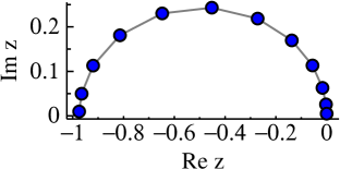
Figure 6: Representative contour integration for occupied states. Twelve points are taken for the interval ($-1,0$). The contour deformation has eccentricity = 1/2, and a bunching parameter 1/2, giving more weight to the points near $E_{F}=0$.

Many properties of interest involve integration over the occupied states. In contrast to band methods which give eigenfunctions for the entire energy spectrum at once, Green’s functions are solved at a particular energy, and must be numerically integrated on an energy mesh for integrated properties. The spectral function or density of states is related to $G$ as

$$A(\varepsilon)=\pi^{-1}|\text{Im}\,G(\varepsilon)|$$ (70)

and in the noninteracting case is comprised of a superposition of $\delta$-functions at the energy levels. Thus $G(\varepsilon)$ has lots of structure on the real axis, which makes integration along it difficult. However, since below the Fermi level $G$ should have no poles in the upper half of the complex plane, the Cauchy theorem can be used to deform the integral from the real axis to a path in the complex plane (Fig. 6). lmgf and lmpg use an elliptical path, with upper and lower bounds on the real axis respectively at the Fermi level and some energy below the bottom of the band.

A Legendre quadrature is used, but the weights can be staggered to bunch points near $E_{F}$ where $G$ has lots of structure. Thus five parameters define the mesh: the number of points, the upper and lower bounds, the eccentricity of the ellipse (between 0 for circle and 1 for a line on the real axis) and bunching parameter which also ranges between 0 and 1. The integrand on the contour is smooth, except near the endpoint $z{\to}E_{F}$. Good results can be obtained with a modest number of points, typically 12-20.

The exact potential function $P^{\alpha}$ has no poles in this half plane; nor does the second order parameterisation but spurious poles may appear in the third order parameterisation. These may be avoided by working in the orthogonal representation ($\alpha=\gamma$) and/or by choosing fairly large elliptical eccentricities for the contour.

2.16 Spin-orbit Coupling in the Green’s Function

It has been shown in Sec. 2.8.2 that spin-orbit coupling (SOC) can be added perturbatively to the Hamiltonian, resulting in the matrix elements containing $\xi_{\ell}[D^{\prime},D]$. These matrix elements are added to the right-hand-side of the first line in Eq. (26), while the overlap integrals (second line in Eq. (26)) remain unchanged. In order to construct the Green’s function with SOC, the resulting modification of the variational energy in Eq. (27) needs to be reformulated as a perturbation of the potential parameters.

Because the SOC operator is a matrix (see Sec. 2.8.2), the exact solutions $\phi_{\nu lj\kappa}(\mathbf{r})$ of the radial Pauli equation are linear combinations of spherical waves $|lm\sigma\rangle$ and $|lm^{\prime}\sigma^{\prime}\rangle$ with $m+\sigma=m^{\prime}+\sigma^{\prime}=j$. However, our perturbative treatment is still based on basis functions with definite spin that are calculated without SOC. The energy dependence, however, is modified by allowing the $\omega$ parameter to become a matrix, so that Eq. (25) is replaced by

$$\Phi_{m\sigma}(D_{\uparrow},D_{\downarrow},{{\mathbf{r}}})=\phi_{m\sigma}(\epsilon_{\nu\sigma},{{\mathbf{r}}})\\ +\sum_{m^{\prime}\sigma^{\prime}}\omega_{m\sigma,m^{\prime}\sigma^{\prime}}(D_{\uparrow},D_{\downarrow})\dot{\phi}_{m^{\prime}\sigma^{\prime}}(\epsilon_{\nu\sigma^{\prime}},{{\mathbf{r}}})$$ (71)

where we dropped the common $\ell$ superscript because the SOC operator is diagonal in $\ell$. The summation in (71) involves at most two terms with $m+\sigma=m^{\prime}+\sigma^{\prime}$.

Instead of the simple variational estimate of $\epsilon(D)$ in Eq. (27), we now construct a generalised eigenvalue equation, which leads to

$$\hat{\omega}+\hat{V}_{\text{SO}}=\epsilon\hat{1}-\hat{\epsilon}_{\nu}+\hat{\omega}^{\dagger}\hat{p}(\epsilon\hat{1}-\hat{\epsilon}_{\nu})\hat{\omega}$$ (72)

where $\hat{\omega}$ is the matrix from Eq. (71), both $\hat{\omega}$ and $\hat{V}_{\text{SO}}$ are functions of $D_{\uparrow}$ and $D_{\downarrow}$, and $\hat{p}$ and $\hat{\epsilon}_{\nu}$ are diagonal matrices with elements $\langle\dot{\phi}^{2}_{\nu\ell\sigma}\rangle$ and $\epsilon_{\nu\sigma}$, respectively. The matrices are assumed to include the full basis set on the given site, i.e., their dimension is $2(2\ell+1)$.

The $\hat{\omega}$ matrix is found by solving Eq. (72). To first order in $\epsilon-\epsilon_{\nu}$, it gives $\hat{\omega}=\epsilon\hat{1}-\hat{\epsilon}_{\nu}-\hat{V}_{\text{SO}}$, so that the matrix elements of $\hat{V}_{\text{SO}}$ are effectively added to $\hat{\epsilon}_{\nu}$. Promoting the potential function $P(\epsilon)$ to a matrix and using the representation Eq. (32) and the definitions Eqs. (29-31), we find that the parameters $\Delta$ and $\gamma$ are unaffected by $\hat{V}_{\text{SO}}$ while $C$ is promoted as $C\to\hat{C}=C\hat{1}+\hat{V}_{\text{SO}}$. However, in order to make the definition of $\hat{P}(\epsilon)$ unambiguous, we need to fix the correct order of matrix multiplication. We also need to ensure that the poles of $G(z)$ have unit residues. We use the following definitions:

$$G(\epsilon) =\lambda(\epsilon)+\mu_{L}(\epsilon)[P(\epsilon)-S]^{-1}\mu_{R}(\epsilon),$$ (73)

$$P(\epsilon) =\left[\gamma+\sqrt{\Delta}(\epsilon-\hat{C})^{-1}\sqrt{\Delta}\right]^{-1}$$ (74)

$$\mu_{L}(\epsilon) =(1-\hat{\dot{V}}_{\text{SO}})^{1/2}[\Delta+\gamma(\epsilon-\hat{C})]^{-1}\sqrt{\Delta}$$ (75)

$$\mu_{R}(\epsilon) =\sqrt{\Delta}[\Delta+(\epsilon-\hat{C})\gamma]^{-1}(1-\hat{\dot{V}}_{\text{SO}})^{1/2}$$ (76)

$$\lambda =-\frac{1}{2}\mu_{R}^{-1}\ddot{P}\mu_{L}^{-1}$$ (77)

where $\hat{\dot{V}}_{\text{SO}}=d\hat{\dot{V}}_{\text{SO}}/d\epsilon$ comes from the energy dependence of the SOC parameters $\xi_{\ell}[D^{\prime},D]$. Note that $\dot{P}=\mu_{R}\mu_{L}$, and the structure of $G(z)$ guarantees that the poles of $G(z)$ have unit residues. It is straightforward to check that, with energy-independent $\hat{V}_{\text{SO}}$, $G(z)$ becomes the resolvent of the second-order Hamiltonian Eq. (37), with added $\hat{V}_{\text{SO}}$, as expected.

To third order in $\epsilon-\epsilon_{\nu}$ and to first order in $\hat{V}_{\text{SO}}$, we find from Eq. (72):

$$\hat{\omega}^{(3)} =\epsilon\hat{1}-\hat{\epsilon}_{\nu}+\hat{p}(\epsilon\hat{1}-\hat{\epsilon}_{\nu})^{3}-\hat{V}_{\text{SO}}^{(3)}$$

$$=\hat{\epsilon}^{\prime}-\hat{\epsilon}_{\nu}-\hat{V}_{\text{SO}}^{(3)}$$ (78)

where $\epsilon^{\prime}$ is defined in Eq. (35), and

$$\hat{V}_{\text{SO}}^{(3)}=\hat{V}_{\text{SO}}+\bigl{\{}\hat{V}_{\text{SO}},\hat{p}(\epsilon\hat{1}-\hat{\epsilon}_{\nu})^{2}\bigr{\}}$$ (79)

with $\bigl{\{}\hat{A},\hat{B}\bigr{\}}=\hat{A}\hat{B}+\hat{B}\hat{A}$. Because $\hat{V}_{\text{SO}}$ is defined at the fixed values of the logarithmic derivatives, the spin-orbit coupling parameters $\xi_{\ell,\sigma\sigma^{\prime}}$ in $\hat{V}_{\text{SO}}$ are calculated with $\epsilon$ replaced by $\epsilon^{\prime}$:

$$\xi {}_{\ell,\sigma\sigma^{\prime}}(\epsilon)=\langle\phi_{\ell\sigma}|\xi(r)|\phi_{\ell\sigma^{\prime}}\rangle$$

$$+(\epsilon^{\prime}_{\ell\sigma}-\epsilon_{\nu\ell\sigma})\langle\dot{\phi}_{\ell\sigma}|\xi(r)|\phi_{\ell\sigma^{\prime}}\rangle$$

$$+(\epsilon^{\prime}_{\ell\sigma^{\prime}}-\epsilon_{\nu\ell\sigma^{\prime}})\langle\phi_{\ell\sigma}|\xi(r)|\dot{\phi}_{\ell\sigma^{\prime}}\rangle$$

$$+(\epsilon^{\prime}_{\ell\sigma}-\epsilon_{\nu\ell\sigma})(\epsilon^{\prime}_{\ell\sigma^{\prime}}-\epsilon_{\nu\ell\sigma^{\prime}})\langle\dot{\phi}_{\ell\sigma}|\xi(r)|\dot{\phi}_{\ell\sigma^{\prime}}\rangle$$ (80)

Of course, just as in the non-relativistic case, $\epsilon$ is also replaced by $\epsilon^{\prime}$ where it appears explicitly in Eqs. (74-76). $\hat{\dot{V}}_{\text{SO}}$ is always calculated as the exact energy derivative of $\hat{V}_{\text{SO}}$.

Figure 7 shows the comparison of the magnetocrystalline anisotropy calculated using lm and lmgf for two benchmark systems. Two cases are displayed: lmgf with second-order potential functions compared with the corresponding two-centre approximation in lm, and lmgf with third-order potential functions compared with the full three-centre lm calculation. The agreement in both cases for FePt [panel (a)] is very good, while for the (Fe_1-xCo_x)₂B alloy in the virtual crystal approximation it is essentially perfect.

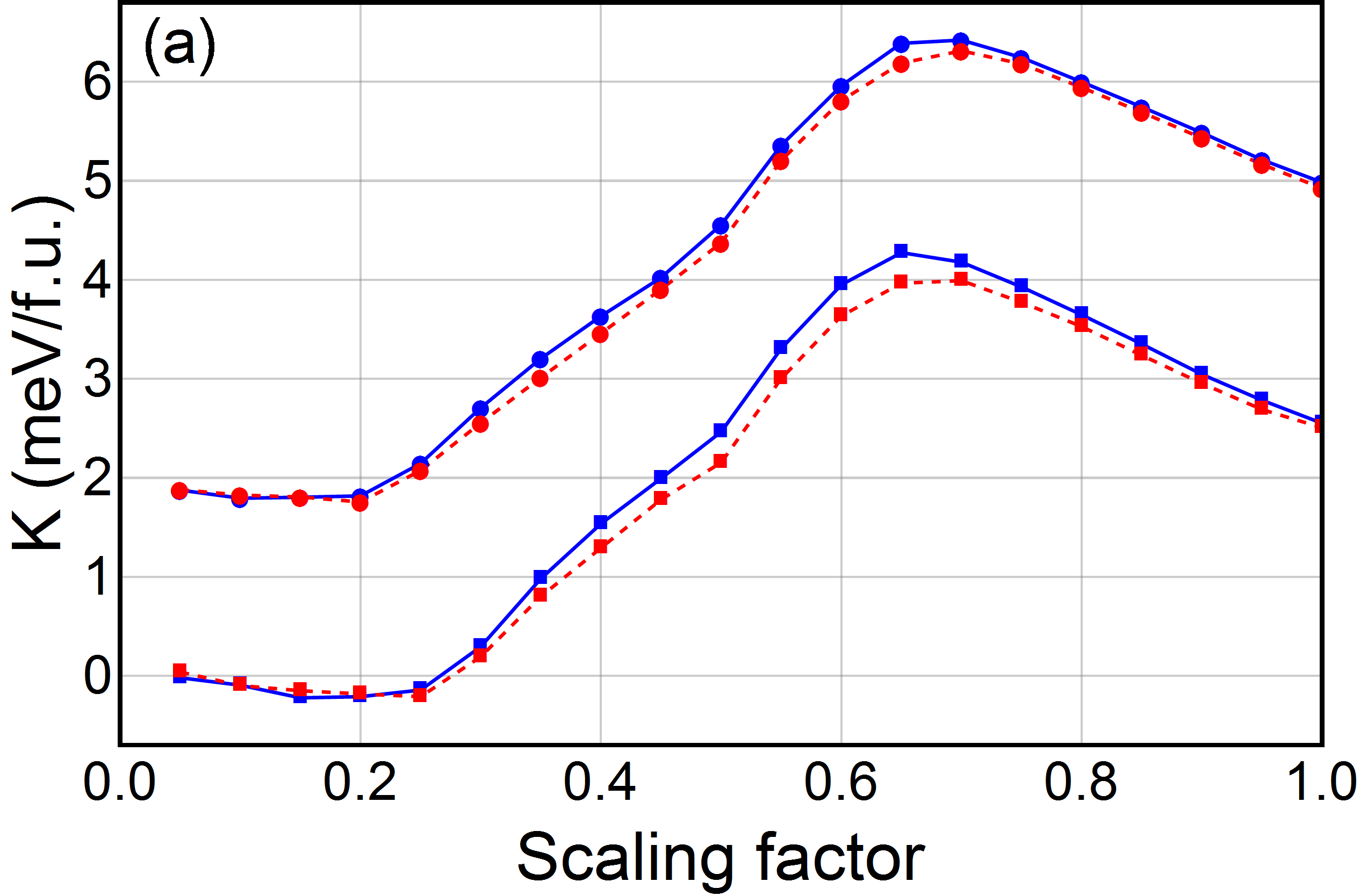
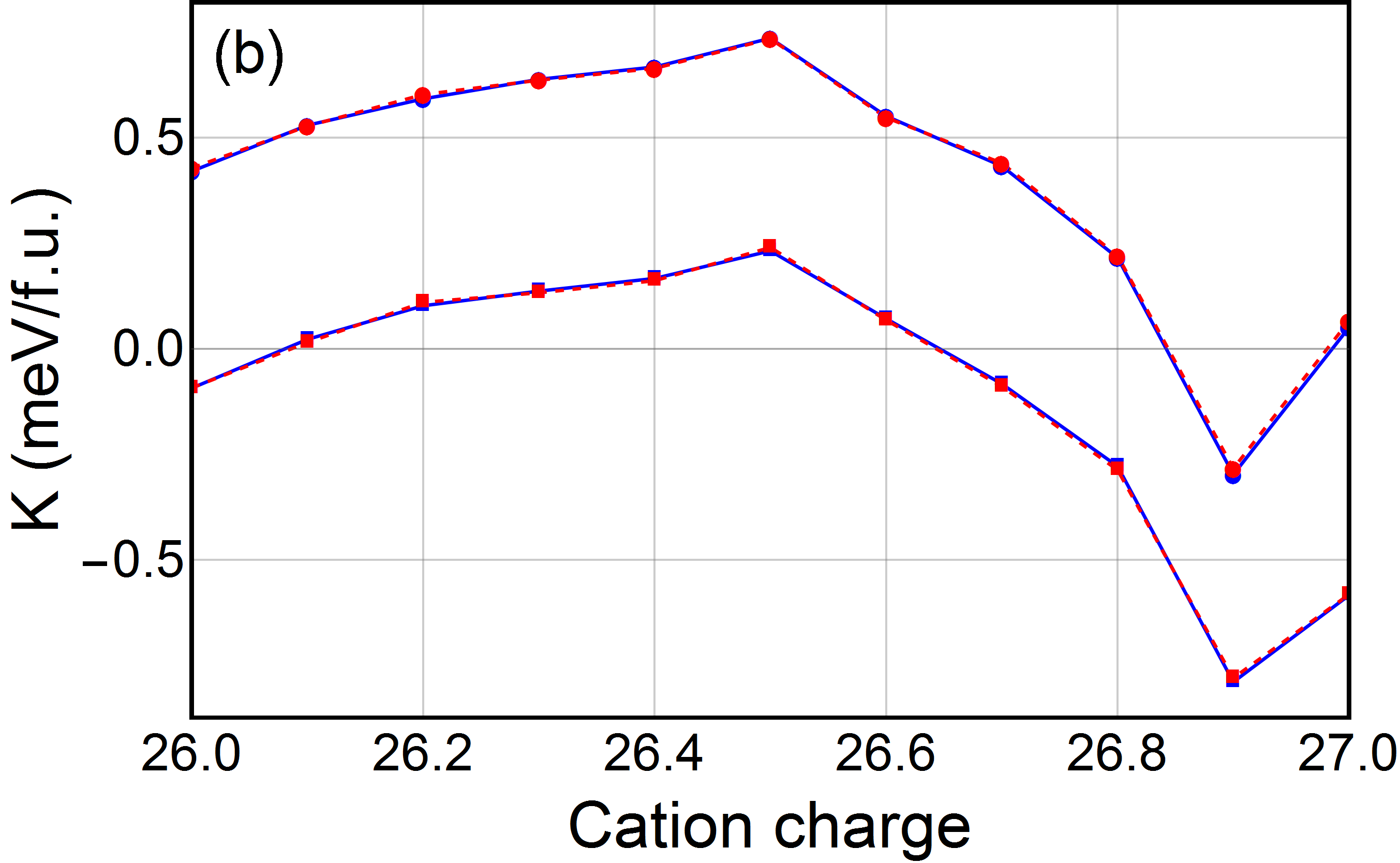
Figure 7: Benchmarks for magnetocrystalline anisotropy using lm (blue symbols and solid curves) and lmgf (red symbols and dashed curves). (a) FePt with the magnetic part of the exchange-correlation field scaled by a factor between 0 and 1. (b) (Fe_1-xCo_x)₂B alloy in the virtual crystal approximation, with the cation charge varied from 26 to 27. Lower curves with squares: full three-centre lm and lmgf with third-order potential functions. Upper curves (shifted by 2 meV/f.u. in panel (a) and by 0.5 meV/f.u. in panel (b)): two-centre approximation in lm and second-order potential functions in lmgf. The charge density in all calculations for the given material is taken from the full self-consistent lm calculation (without scaling in the case of FePt).

2.17 Fully Relativistic LMTO-ASA

We have developed a fully relativistic extension of the LMTO-ASA code within a relativistic generalisation of the density functional formalism [39, 40, 41, 42, 43]. In the most general case, one needs to solve the Kohn-Sham Dirac equation

$$H\Psi(\varepsilon,{\mathbf{r}})=\varepsilon\Psi(\varepsilon,{\mathbf{r}})$$ (81)

with

$$H=c{\mathbf{\alpha}}{\mathbf{p}}+(\beta-I_{4})mc^{2}+V({\mathbf{r}})I_{4}+\mu_{B}\beta{\mathbf{B}}_{\text{eff}}({\mathbf{r}}){\mathbf{\Sigma}}$$ (82)

where

$$\alpha=\begin{pmatrix}0&{\mathbf{\sigma}}\\ {\mathbf{\sigma}}&0\end{pmatrix},\;\beta=\begin{pmatrix}I_{2}&0\\ 0&-I_{2}\end{pmatrix},\;\Sigma=\begin{pmatrix}{\mathbf{\sigma}}&0\\ 0&{\mathbf{\sigma}}\end{pmatrix}\;$$ (83)

Here, ${\mathbf{\sigma}}$ is the vector of Pauli matrices, ${\mathbf{p}}$ is the momentum operator, ${\mathbf{B}}_{\text{eff}}({\mathbf{r}})$ is an effective spin-dependent potential acting on electrons. It should be noted that this is a simplified form of the relativistic Kohn-Sham equation in which the orbital contribution to the 4-component relativistic current is neglected. This simplification is necessary in order to avoid the significant formulaic and computational complications that arise in the relativistic current density formulation of the density functional theory [43].

For a spherically symmetric potential $V(r)=1/2[V_{\uparrow}(r)+V_{\downarrow}(r)]$ inside a single MT sphere, the direction of the magnetic field can be assumed to point along the $z$ direction, ${\mathbf{B}}_{\text{eff}}=B(r)\hat{z}$, where $B(r)=1/2[V_{\uparrow}(r)-V_{\downarrow}(r)]$. Then, Eq. (82) can be written as

$$H=[c{\mathbf{\alpha}}{\mathbf{p}}+(\beta-I_{4})mc^{2}+V(r)I_{4}+\mu_{B}\beta B(r)\Sigma_{z}]$$ (84)

The solutions of the Kohn-Sham Dirac equation (84) are linear combinations of bispinors:

$$\Psi_{\mu}({\mathbf{r}},\varepsilon)=\sum_{\kappa}\Psi_{\kappa\mu}({\mathbf{r}},\varepsilon)$$ (85)

$$\Psi_{\kappa\mu}({\mathbf{r}},\varepsilon)=\begin{pmatrix}g_{\kappa\mu}(\varepsilon,r)\Omega_{\kappa\mu}(\hat{r})\\ if_{\kappa\mu}(\varepsilon,r)\Omega_{-\kappa\mu}(\hat{r})\end{pmatrix}$$ (86)

Here, $\Omega_{\kappa\mu}(\hat{r})$ are the spin spherical harmonics, $\mu$ is the projection of the total angular momentum, and $\kappa$ is the relativistic quantum number, $\kappa^{2}=J(J+1)+1/4$. The radial amplitudes $g_{\kappa\mu}(\varepsilon,r)$ and $f_{\kappa\mu}(\varepsilon,r)$ satisfy the following set of coupled differential equations:

$$\left[\frac{d}{dr}+\frac{1+\kappa_{1}}{r}\right]g_{\kappa_{1}\mu}(\varepsilon,r)=\\ \left[1+\frac{\varepsilon-V(r)+u{{}^{\prime}}B(r)}{c^{2}}\right]cf_{\kappa_{1}\mu}(\varepsilon,r)$$

$$\left[\frac{d}{dr}+\frac{1-\kappa_{1}}{r}\right]cf_{\kappa_{1}\mu}(\varepsilon,r)=\\ \left[-\left(\varepsilon-V(r)\right)-uB(r)\right]cg_{\kappa_{1}\mu}(\varepsilon,r)\\ -\sqrt{1-u^{2}}B(r)g_{\kappa_{2}\mu}(\varepsilon,r)$$

$$\left[\frac{d}{dr}+\frac{1+\kappa_{2}}{r}\right]g_{\kappa_{2}\mu}(\varepsilon,r)=\\ \left[1+\frac{\varepsilon-V(r)+u{{}^{\prime\prime}}B(r)}{c^{2}}\right]cf_{\kappa_{2}\mu}(\varepsilon,r)$$

$$\left[\frac{d}{dr}+\frac{1-\kappa_{2}}{r}\right]cf_{\kappa_{2}\mu}(\varepsilon,r)=\\ \left[-\left(\varepsilon-V(r)\right)-uB(r)\right]cg_{\kappa_{2}\mu}(\varepsilon,r)\\ -\sqrt{1-u^{2}}B(r)g_{\kappa_{1}\mu}(\varepsilon,r)$$ (87)

where

$$u=\frac{\mu}{\ell+1/2},\quad u{{}^{\prime}}=\frac{\mu}{\ell-1/2},\quad u{{}^{\prime\prime}}=\frac{\mu}{\ell+3/2}$$ (88)

In the general case, in the presence of a magnetic field, one has to solve a system of two infinite sets of mutually coupled differential equations because the magnetic field couples radial amplitudes with different relativistic quantum numbers $\kappa$. Specifically, states with $\kappa_{1}$ to those with $\kappa_{2}=\kappa_{1}$ and $\kappa_{2}=-\kappa_{1}-1$, i.e., states of the same $\ell$, but also states with $\kappa_{1}$ to those with $\kappa_{2}=1-\kappa_{1}$, i.e., states with different $\ell$’s, $\Delta\ell=\pm 2$. To avoid this complication, this coupling is neglected. In this case, the set simplifies into coupled equations for each pair $\ell\mu$. For $|\mu|=\ell+1/2$, there is no coupling, so similar to the non-relativistic case, there is only regular solution with quantum numbers $\kappa\mu$, while for $|\mu|<\ell+1/2$, we need to solve the set of four coupled equations (87) for the four unknown radial functions $g_{\kappa_{1}\mu}$, $f_{\kappa_{1}\mu}$, $g_{\kappa_{2}\mu}$, and $f_{\kappa_{1}\mu}$. The coefficients $u$, $u^{{}^{\prime}}$, and $u{{}^{\prime\prime}}$ in Eq. (87) result from matrix elements of the type $\langle\kappa\mu|\sigma_{z}|\kappa^{{}^{\prime}}\mu\rangle$ [43].

Physically, the neglected coupling corresponds to a magnetic spin-orbit interaction given by a term $2c^{-2}r^{-1}dB/dr{\mathbf{L}}\cdot{\mathbf{S}}$ in the weak relativistic domain [44]. Since this is proportional to the product of two small quantities ($c^{-2}$ and $dB/dr$) its omission is justified in most cases.

The construction of the MT orbitals and the corresponding boundary conditions proceeds along the same principles as in the non-relativistic case described in the previous sections. The tail cancellation condition is conveniently formulated in terms of relativistic extensions of the potential and normalisation functions:

$$N_{\mathcal{L}}(\varepsilon)=(2\ell+1)\left(\frac{w}{s}\right)^{\ell+1}g_{\mathcal{L}}^{-1}(\varepsilon,s)\\ \times\left(D_{\mathcal{L}}(\varepsilon,s)-I\ell\right)^{-1}$$ (89)

$$P_{\mathcal{L}}(\varepsilon)=2(2\ell+1)\left(\frac{w}{s}\right)^{2\ell+1}\\ \times\left(D_{\mathcal{L}}(\varepsilon,s)+I_{\ell}+I\right)\left(D_{\mathcal{L}}(\varepsilon,s)-I\ell\right)^{-1}$$ (90)

The logarithmic derivative matrix being given in terms of the small and large components of the radial amplitude:

$$D_{\mathcal{L}}(\varepsilon,r)=scf_{\mathcal{L}}(\varepsilon,s)g_{\mathcal{L}}^{-1}(\varepsilon,s)-\kappa-I$$ (91)

$$\kappa=\begin{pmatrix}\kappa_{1}&0\\ 0&\kappa_{2}\end{pmatrix}$$

For states with $|\mu|<\ell+1/2$, $N_{\mathcal{L}}(\varepsilon)$, $P_{\mathcal{L}}(\varepsilon)$, $D_{\mathcal{L}}(\varepsilon)$, $g_{\mathcal{L}}(\varepsilon)$, and $f_{\mathcal{L}}(\varepsilon)$ are 2$\times$2 matrices for each subblock $\mathcal{L}=(\ell,\mu)$ with the general form

$$A_{\mathcal{L}}(\varepsilon)=\begin{pmatrix}A_{\alpha_{1}\kappa{1}}(\varepsilon)&A_{\alpha_{1}\kappa_{2}}(\varepsilon)\\ A_{\alpha_{2}\kappa{1}}(\varepsilon)&A_{\alpha_{2}\kappa_{2}}(\varepsilon)\end{pmatrix}$$ (92)

Note that the indices in this matrix have different physical meaning. Although the values of index $\alpha$ are numerically equal to those of $\kappa$, index $\alpha$ stands for different behaviour of the radial function at the origin [42, 43] while $\kappa$ stands for solutions with different quantum states. Therefore, these matrices are not symmetric and do not commute with each other.

The linearisation can be formulated in a matrix form too [in the following we will leave out the subblock index $\mathcal{L}$; all presented matrices have the form of Eq. (92)]. Within second-order approximation, the radial amplitudes are expanded around a linearisation energy:

$$g(\varepsilon,r)\approx g_{\nu}(r)+\left(\varepsilon-\varepsilon_{\nu}\right)I\dot{g_{\nu}}(r)$$ (93)

$$f(\varepsilon,r)\approx f_{\nu}(r)+\left(\varepsilon-\varepsilon_{\nu}\right)I\dot{f_{\nu}}(r)$$ (94)

Then, a symmetric matrix form of the linearisation of the logarithmic derivative can be written as

$$\left(D(\varepsilon)-D_{\nu}\right)^{-1}=-\frac{s}{\epsilon}g_{\nu}g_{\nu}^{T}+A$$ (95)

where

$$A =-\frac{1}{2}\left[\left(D_{\nu}-D_{\dot{\nu}}\right)^{-1}+\left(D_{\nu}-D_{\dot{\nu}}^{T}\right)^{-1}\right]$$

$$=-\frac{1}{2}s\left(\dot{g}_{\nu}g_{\nu}^{T}+g_{\nu}\dot{g}_{\nu}^{T}\right)$$ (96)

By direct substitution of (95) into (90) we obtain the parameterisation of the potential function:

$$P(\varepsilon)=R\left(V-\varepsilon\right)^{-1}R^{T}+Q$$ (97)

or equivalently

$$P^{-1}(\varepsilon)=W\left(C-\varepsilon\right)^{-1}W^{T}+\gamma$$ (98)

where

$$V=\varepsilon_{\nu}+sg_{\nu}^{T}\left[A+\left(D_{\nu}-Il\right)^{-1}\right]^{-1}g_{\nu}$$ (99)

$$R=\sqrt{2s}\left(\frac{w}{s}\right)^{\ell+\frac{1}{2}}\left(2\ell+1\right)\left[A\left(D_{\nu}-Il\right)+I\right]^{-1}g_{\nu}$$ (100)

$$Q=2\left(2\ell+1\right)\left(\frac{w}{s}\right)^{2\ell+1}\\ \times\left[I+\left(2\ell+I\right)\left[\left(D_{\nu}-Il\right)+A^{-1}\right]^{-1}\right]$$ (101)

and

$$\gamma=Q^{-1},\quad W=\gamma R,\quad C=V+R^{T}\gamma R$$ (102)

For an arbitrary representation $\alpha$:

$${P^{\alpha}}^{-1}(\varepsilon)=W\left(C-\varepsilon\right)^{-1}W^{T}+\gamma-\alpha$$ (103)

which is the relativistic analogue of Eq. (48). In general, the matrices $V$, $R$, $Q$, $C$, $\gamma$ and $W$ are non-diagonal, some are symmetric and some are not, so they do not all commute with each other. This is related to the different physical origin of the matrix indices discussed above. The parameter $W$ is the relativistic analogue of $\sqrt{\Delta}$ introduced earlier [see Eq. (33)], and Eq. (97) is analogous to the non-relativistic Eq. (32). We should note that in the code, we have also included a third-order parameterisation of the potential function similar to the non-relativistic case, Eq. (35).

The physical Green function and Hamiltonian are written in terms of the potential function and scalar relativistic structure constants matrices after a transformation of the former from $\kappa\mu$ to $\ell mm_{s}$ basis:

$$G^{\alpha}=-\frac{1}{2}\ddot{P}^{\alpha}\dot{P}^{\alpha}+\frac{2}{w}{N^{\alpha}}^{T}g^{\alpha}N^{\alpha}$$ (104)

where

$$g^{\alpha}=\left(P^{\alpha}-S^{\alpha}\right)^{-1}$$ (105)

these are the relativistic analogues of Eq (57) and the scattering path operator.

Within the framework of the TB-LMTO and principal layer approach, the fully relativistic version of the green function for layered geometry is constructed straightforwardly from the site diagonal fully relativistic potential function [43].

2.18 Coherent Potential Approximation

The coherent potential approximation (CPA) is a Green’s function-based method used to describe the electronic structure of disordered substitutional alloys. Questaal’s lmgf code implements the CPA in the Atomic Spheres Approximation, following the formulation of Refs. [45, 43]. Any lattice site $i$ can be occupied by any number of components $a$ with probabilities (concentrations) $c^{a}_{i}$, which must be supplied by the user. These components can have different atomic sphere radii, and each has its own charge density, atomic potential, and diagonal matrix of potential functions $P^{a}_{i}(\epsilon)$. Each site with substitutional disorder (“CPA site”) is also assigned a coherent potential matrix $\EuScript{P}_{i}(\epsilon)$ that has the same orbital structure as $P^{a}_{i}(\epsilon)$ but is off-diagonal, with the restriction that it must be invariant under its site’s point group. The elements of the $\EuScript{P}_{i}(\epsilon)$ matrix are complex even if $\epsilon$ is real, and it is fixed by the CPA self-consistency condition.

The configurational average of the scattering path operator is given by

$$\bar{g}(\epsilon,\mathbf{k})=[\EuScript{P(\epsilon)}-S(\mathbf{k})]^{-1}$$ (106)

where the site-diagonal matrix $\EuScript{P}(\epsilon)$ absorbs the coherent potential matrices for the CPA sites and the diagonal matrices of the conventional potential functions for the sites that are occupied deterministically (“non-CPA sites”). The matrix in Eq. (106) is integrated over the Brillouin zone in the usual way, and its site-diagonal blocks $\bar{g}_{ii}$ are extracted.

For non-CPA sites, the full Green’s function, density matrix, and the charge density are obtained from $\bar{g}_{ii}$ in the usual way. For each CPA site $i$, we define the scattering path operator $\bar{g}^{a}_{i}$ (separately for each component $a$), which is the statistical average under the restriction that site $i$ is occupied deterministically by component $a$, while all other sites in the infinite crystal are occupied statistically, according to their average concentrations. Such quantities are called “conditionally averaged.” The charge density for the component $a$ on site $i$ is obtained from the site-diagonal block $\bar{g}^{a}_{ii}$ on site $i$ of the conditionally averaged $\bar{g}^{a}_{i}$. This site-diagonal block can be found from the matrix equation on that site:

$$(\bar{g}^{a}_{ii})^{-1}=\bar{g}_{ii}^{-1}+P^{a}_{i}-\EuScript{P}_{i}$$ (107)

and the CPA self-consistency condition reads

$$\bar{g}_{ii}=\sum_{i}c^{a}_{i}\bar{g}^{a}_{ii}$$ (108)

Iteration to self-consistency is facilitated [45, 43] by introducing the coherent interactor matrix $\Omega_{i}$, for each CPA site, defined through $\bar{g}_{ii}=(\EuScript{P}_{i}-\Omega_{i})^{-1}$. The conditionally averaged $\bar{g}^{a}_{ii}$ is then $\bar{g}^{a}_{ii}=(P^{a}_{i}-\Omega_{i})^{-1}$. The latter two equations can be used to re-express the self-consistency condition (108) in terms of $\EuScript{P}_{i}$, $\Omega_{i}$, and $P^{a}_{i}$ without an explicit reference to the scattering path operator:

$$(\EuScript{P}_{i}-\Omega_{i})^{-1}=\sum_{i}c^{a}_{i}(P^{a}_{i}-\Omega_{i})^{-1}$$ (109)

The $\Omega_{i}$ matrices (for each required complex energy point) are converged to self-consistency using the following procedure. At the beginning of the CPA iteration, Eq. (109) is used to obtain $\EuScript{P}_{i}$ for each CPA site from $\Omega_{i}$, and then $\EuScript{P}_{i}$ is inserted in Eq. (106). After integration over $\mathbf{k}$, the site-diagonal block $\bar{g}_{ii}$ is extracted for each CPA sites and used to obtain the next approximation for $\Omega_{i}=\EuScript{P}_{i}-\bar{g}_{ii}^{-1}$, closing the self-consistency loop. The output $\Omega_{i}$ matrices are linearly mixed with their input values. The mixing parameter can usually be set to 1 for energy points that are not too close to the real axis.

The CPA loop is repeated until the $\Omega_{i}$ matrices converge to the desired tolerance, after which a charge iteration is performed. At the beginning of the calculation, the $\Omega_{i}$ matrices are initialised to zero unless they have already been stored on disk. The CPA loop can sometimes converge to an unphysical symmetry-breaking solution; this can usually be avoided by symmetrising the coherent potentials using the full space group of the crystal.

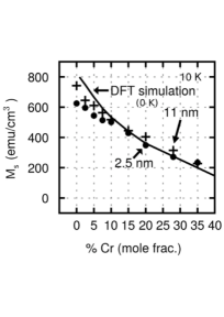
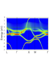
Figure 8: Left: DFT magnetic moment in (Ni₈₀Fe₂₀)_1-xCr_x, compared to experiment (films with 11 nm (crosses) and 2.5 nm (dots) thickness) at 10K. Right: Majority-spin CPA spectral function at $x$=20%. Adapted from Ref. [46] and Vishina’s PhD thesis [47].

Fig. 8 illustrates one recent application of Questaal’s implementation of the CPA. A number of new, potentially high-impact technologies, Josephson MRAM (JMRAM) in particular, performs write operations by rotating a patterned magnetic bit. These operations consume a significant portion of a system’s power. One way to reduce the power consumed by write operations is to substitute materials with smaller saturation magnetisation $M_{s}$. The minimum usable $M_{s}$ is limited by the need to maintain large enough energy barrier to prevent data loss due to thermal fluctuations. Low $M_{s}$ can greatly reduce power particularly for JMRAM [48], which operates at around 4 K. One way to reduce $M_{s}$ in permalloy (Ni₈₀Fe₂₀ alloys, the most commonly used JMRAM material), is to admix Cr into it, as Cr aligns antiferromagnetically to Fe and Ni. Fig. 8 shows some results adapted from a recent joint experimental and theoretical study of Py_1-xCr_x, [46]. The CPA calculations of $M_{s}$ track measured values fairly well. Also shown is the CPA energy band structure for the majority spin. Alloy scattering causes bands to broaden out, and scattering lifetimes can be extracted. A detailed account can be found in Vishina’s PhD thesis [47].

2.19 Noncollinear Magnetism

The ASA codes lm, lmgf and lmpg are fully noncollinear in a rigid-spin framework, meaning that the spin quantisation axis is fixed within a sphere, but each sphere can have its own axis. The formulation is a straightforward generalisation of the nonmagnetic case. Potential and Hamiltonian-like objects become $2{\times}2$ matrices in spin space. The structure matrix $S$ is diagonal matrix in this space and independent of spin, while potential functions $P$ and potential parameters of Sec. 2.8.1, become $2{\times}2$ matrices that are diagonal in $\ell$ but off-diagonal in spin. (Alternatively, a local spin quantisation axis can be defined which makes $P$ diagonal in spin; then $S$ is no longer diagonal.) How Questaal constructs the Hamiltonian in the general noncollinear case, and also for spin spirals, is discussed in Ref. [49].

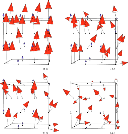
Figure 9: Self-consistent magnetic spin configurations of the fcc Fe-Ni alloy at the four volumes 78.8, 73.7, 71.9, and 68.6 a.u.. Red and blue arrows show magnetic moments on Fe and Ni atoms, respectively. Taken from Ref. [50].

These codes have implemented spin dynamics [11], integrating the Landau-Lifshitz equation using a solver from A. Bulgac and D. Kusnezov [51], the spin analogue of molecular dynamics and molecular statics. The formulation is described in detail in Ref. [49]. Codes also implement spin statics. Torques needed for both are obtained in DFT from the off-diagonal parts of the spin-density matrix. A classic application is the study of INVAR. Fe-Ni alloys with a Ni concentration around 35 atomic % (INVAR) exhibit anomalously low, almost zero, thermal expansion over a considerable temperature range. In Ref. [50] it was shown that at 35% composition, Fe-Ni alloys are on the cusp of a collinear-noncollinear transition, and this adds a negative contribution to the Grüneisen parameter. Fig. 9 is reproduced from that paper.

3 Full Potential Implementation

Questaal’s primary code lmf is an augmented-wave implementation of DFT without shape approximations. It also handles the one-body part of the quasiparticle self-consistent GW approximation, by adding the (quasiparticlised) GW self-energy to the DFT part. Closely related codes are lmfgwd, a driver supplying input for the GW, lmfdmft, a driver supplying input for a DMFT solver, and lmfgws, a post-processing tool that generates quantities using the one-body part from lmf and the dynamical self-energy from GW or DMFT. This code uses different definitions for classical functions (see Appendix B), and we shift to those definitions in what follows.

As for the DFT part, Questaal’s unique features are:

• it uses a three-component augmentation, following most of the original method of Ref. [31]. The augmentation is reviewed in Sec. 3.6. Ref. [52] offers a slightly different presentation and shows how it is connected with the PAW method [4].

• it has a more general basis set. Ordinary Hankel functions solve Schrödinger’s equation for a MT potential, but real potentials vary smoothly into the interstitial (Fig. 10). The envelope function of a minimal basis set must adapt to this potential. The traditional Questaal basis uses smooth Hankel functions [53], which may be thought of as a convolution of a Gaussian function and a traditional Hankel function; they are developed in Sec. 3.1. This traditional basis works very well for most systems; however when the system is very open, it is slightly incomplete (Sec. 3.13). One way to surmount the incompleteness is to combine smooth Hankel functions with plane waves; this is the “Plane-wave Muffin Tin” (PMT) basis [54] (see also Ref. [52]). While it would seem appealing, PMT suffer from two serious drawbacks: first, it tends to become over-complete even with a relatively small number of plane waves, and second, it is not compact (minimal, short ranged and as complete as possible for the relevant energy window).

• Questaal’s most recent development is the “Jigsaw Puzzle Orbital” (JPO) basis, which uses information from the augmentation to construct an optimal shape for the envelope functions. To the best of our knowledge, JPO’s are the closest practical realisation of compactness. This is particularly important in many-body treatments where the efficacy of a theory hinges critically on compactness. This new basis will be presented more fully elsewhere. In Sec. 3.12 we show how a transformation to a tight-binding representation can be carried out in a full-potential framework. In the present version the basis set is merely a unitary transformation of the original one.

3.1 Smooth Hankel Functions

In his PhD dissertation Michael Methfessel introduced a class of functions $\mathcal{H}_{kL}(E,r_{s},{{\mathbf{r}}})$. As limiting cases they encompass both ordinary Hankel functions and Gaussian functions (see Eq. (123) and (125) below). They are explained in detail in Ref. [53]; here we present enough information for development of the Questaal basis set. They are all connected to the smooth Hankel function for ${\ell{=}0}$. Its Fourier transform is

$$\widehat{h}_{0}(E,r_{s};{q})=-\frac{4\pi}{E-q^{2}}e^{r_{s}^{2}(E-q^{2})/4}$$ (110)

which is a product of Fourier transforms of ordinary Hankel function for ${\ell{=}0}$ with a Gaussian function of width $2/r_{s}$.

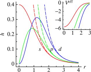
Figure 10: Radial part of smooth Hankel functions $\mathcal{H}_{L}$ for $s$, $p$, $d$ orbitals (solid lines) and corresponding ordinary Hankel functions $H_{L}$ (dashed lines). Smoothing radius and energy were chosen to be $r_{s}=+1$ and $E=-1$, respectively. For $r{\gg}r_{s}$, $\mathcal{H}_{L}\,{\to}\,H_{L}$, while for $r{\ll}r_{s}$, $\mathcal{H}_{L}\,{\propto}\,r^{\ell}$ and ${H}_{L}\,{\propto}\,r^{-\ell-1}$. The ${H}_{L}$ satisfy the Helmholtz wave equation (Schrödinger equation for constant potential), while the $\mathcal{H}_{L}$ satisfy a Schrödinger equation corresponding to a potential $V^{\text{eff}}=-4\pi G_{L}/\mathcal{H}_{L}$, as shown in the inset.

We use standard definitions of Fourier transforms

$$\widehat{f}({{{\mathbf{q}}}}) =\int{{e^{-i{{{\mathbf{q}}}}\cdot{{{\mathbf{r}}}}}}}f({{{\mathbf{r}}}})\,d^{3}r$$

$${f}({{{\mathbf{r}}}}) =\frac{1}{(2\pi)^{3}}\int{{e^{+i{{{\mathbf{q}}}}\cdot{{{\mathbf{r}}}}}}}\widehat{f}({{{\mathbf{q}}}})\,{d^{3}}q$$ (111)

Thus in real space, ${h}_{0}(E,r_{s};r)$ is a convolution of a ordinary Hankel function and a Gaussian function. It has an analytic representation

$$h_{0}(E,r_{s};r)=\frac{1}{2r}\left(u_{+}-u_{-}\right)$$ (112)

$$\dot{h}_{0}(E,r_{s};r)=\frac{1}{4\bar{\kappa}}\left(u_{+}+u_{-}\right)$$ (113)

$$u_{\pm}=e^{\mp\bar{\kappa}{}r}\left[1-{\rm{erf}}\left(\frac{r_{s}\bar{\kappa}}{2}\mp{}\frac{r}{r_{s}}\right)\right]$$ (114)

$$E=-\bar{\kappa}^{2}{\text{ if }}E<0$$ (115)

For small $r$, $h_{0}$ behaves as a Gaussian and it evolves smoothly into an ordinary Hankel when $r{\gg}r_{s}$. $\dot{h}_{0}$ is the energy derivative of ${h}_{0}$.

Questaal’s envelope functions are generalised Hankel functions ${\mathcal{H}}_{L}(E,r_{s};{{{\mathbf{r}}}})$. Their Fourier representation has a closed form

$$\widehat{\mathcal{H}}_{L}(E,r_{s};{{{\mathbf{q}}}}) =\mathcal{Y}_{L}(-i{{{\mathbf{q}}}})\frac{-4\pi\;}{E-q^{2}}e^{r_{s}^{2}(E-q^{2})/4}$$

$$=\mathcal{Y}_{L}(-i{{{\mathbf{q}}}})\widehat{h}_{0}(E,r_{s};{q})$$ (116)

$\mathcal{Y}_{L}({{{\mathbf{r}}}})$ is a spherical harmonic polynomial (Appendix A). Following the usual rules of Fourier transforms this function has a real-space representation

$$\mathcal{H}_{L}(E,r_{s};{{{\mathbf{r}}}})=\mathcal{Y}_{L}(-\nabla)h_{0}(E,r_{s};r)$$ (117)

$\mathcal{Y}_{L}({{{\mathbf{r}}}}),\ {{{\mathbf{r}}}}=(x,y,z)$ is a polynomial in $(x,y,z)$, so is meaningful to talk about $\mathcal{Y}_{L}(-\nabla)$. The extended family $\mathcal{H}_{kL}({{{\mathbf{r}}}})$ is defined through powers of the Laplacian operator:

$$\widehat{\mathcal{H}}_{kL}(E,r_{s};{{{\mathbf{q}}}}) =(-iq)^{2k}\,{\widehat{\mathcal{H}}_{L}(E,r_{s};{{{\mathbf{q}}}})}$$

$$\mathcal{H}_{kL}(E,r_{s};{{{\mathbf{r}}}}) =\nabla^{2k}\mathcal{H}_{L}(E,r_{s};{{{\mathbf{r}}}})$$ (118)

A recursion relation for $\mathcal{H}_{L}(E,r_{s};{{{\mathbf{r}}}})$ for $\ell{>}0$ can be derived from properties of Fourier transforms in spherical coordinates. Any function whose Fourier transform factors as

$$\hat{F}({{{\mathbf{q}}}})={{\hat{f}(q)}}{Y_{L}}({\mathbf{\hat{q}}})$$ (119)

has a real-space form

$$F({{{\mathbf{r}}}})={{f(r)}}{Y_{L}}({\mathbf{\hat{r}}})$$ (120)

where $f$ and $\hat{f}$ are related by [53]

$$f(r) =\frac{{4\pi{i^{\ell}}}}{{{{(2\pi)}^{3}}}}\int_{0}^{\infty}{q\hat{f}(q)\,{j_{\ell}}(qr)}\,qr\,dq$$

$$\hat{f}(q) =4\pi{(-i)^{\ell}}\int_{0}^{\infty}{rf(r)\,{j_{\ell}}(qr)}\,qr\,dr$$

and $j_{\ell}$ is the spherical Bessel function. We can therefore express $\mathcal{H}_{L}$ in a Slater-Koster form

$$\mathcal{H}_{L}({{{\mathbf{r}}}}) =h_{\ell}(r)\,{Y}_{L}({\hat{{{\mathbf{r}}}}})\equiv\chi_{\ell}(r)\,\mathcal{Y}_{L}({{{\mathbf{r}}}})$$ (121)

$$\chi_{\ell}(r) =(1/r^{\ell})\,h_{\ell}(r)$$ (122)

For envelope functions used in basis sets, e.g. $\mathcal{H}_{L}(E,r_{s};{{{\mathbf{r}}}})$, the radial portion of the Fourier transform does not depend on $\ell$; therefore corresponding real-space part depends on $\ell$ only through the $j_{\ell}$. This is a very useful fact. It is possible to derive a recurrence relation to obtain $\chi_{\ell}$ for $\ell{>}1$; this provides an efficient scheme for calculating them. The recurrence is derived in Ref. [53] (see Eq. 6.21):

$$\chi_{\ell+1}=\frac{{2\ell+1}}{{{r^{2}}}}{\chi_{\ell}}-\frac{E}{{{r^{2}}}}{\chi_{\ell-1}}\\ -\frac{{4\pi}}{r^{2}(\pi r_{s}^{2})^{3/2}}\left(\frac{2}{r_{s}^{2}}\right)^{\ell-1}{e^{r_{s}^{2}E/4-{{(r/{r_{s}})}^{2}}}}$$

$\chi_{0}$ and $\chi_{-1}$ are needed to start the recursion. $\chi_{0}$ is written in Eq. (112) and $\chi_{-1}$ can be obtained by combining Eqs. (113), (137) and (122).

By taking limiting cases we can see the connection with familiar functions, and also the significance of parameters $E$ and $r_{s}$.

• $k{=}r_{s}{=}0$: $\widehat{H}_{0}(E,0;{{{\mathbf{q}}}}){=}-{4\pi/(E-q^{2})}\mathcal{Y}_{00}({{{\mathbf{q}}}})$. This is the Fourier transform of $H_{0}(E,0;r)=\mathcal{Y}_{00}({{{\mathbf{r}}}})\exp(-\bar{\kappa}{}r)/r$, and is proportional to the $\ell{=}0$ spherical Hankel function of the first kind, $h_{\ell}^{(1)}(z)$. For general $L$ the relation defines Questaal’s standard definition of ordinary Hankel functions

  $$H_{L}(E,0;{{{\mathbf{r}}}}) =H_{0L}(E,0;{{{\mathbf{r}}}})$$

  $$=-i^{\ell}\bar{\kappa}^{\ell+1}h_{\ell}^{(1)}(i\bar{\kappa}{}r)\text{Y}_{L}(\hat{{{\mathbf{r}}}})$$ (123)

• $k{=}1$ and $E{=}0$: $\widehat{\mathcal{H}}_{10}(0,r_{s};{{{\mathbf{q}}}})=-{4\pi}e^{-r_{s}^{2}q^{2}/4}$.
  This is the Fourier transform of a Gaussian function of width $r_{s}$. For general $L$ we can define the family as

  $$G_{L}(E,r_{s};{{{\mathbf{r}}}})=\mathcal{Y}_{L}(-\nabla)g(E,r_{s};r)$$ (124)

  $$g(E,r_{s};r)=\left({\pi{}r_{s}^{2}}\right)^{-3/2}e^{E{}r_{s}^{2}/4}e^{-r^{2}/r_{s}^{2}}$$ (125)

Evidently $\widehat{\mathcal{H}}_{L}({{{\mathbf{q}}}})$ is proportional to the product of the Fourier transforms of a conventional spherical Hankel function of the first kind, and a Gaussian. By the convolution theorem, ${\mathcal{H}_{L}}({{{\mathbf{r}}}})$ is a convolution of a Hankel function and a Gaussian. For $r{\gg}r_{s}$, ${\mathcal{H}_{L}}({{{\mathbf{r}}}})$ behaves as a Hankel function and asymptotically tends to $\mathcal{H}_{L}({{{\mathbf{r}}}})\to r^{-\ell-1}\exp(-\sqrt{-E}r)\text{Y}_{L}(\hat{{{\mathbf{r}}}})$. For $r{\ll}r_{s}$ it has structure of a Gaussian; it is therefore analytic and regular at the origin, varying as $r^{\ell}\text{Y}_{L}(\hat{{{\mathbf{r}}}})$. Thus, the $r^{-\ell-1}$ singularity of the Hankel function is smoothed out, with $r_{s}$ determining the radius for transition from Gaussian-like to Hankel-like behaviour. Thus, the smoothing radius $r_{s}$ determines the smoothness of $\mathcal{H}_{L}$, and also the width of $G_{L}$.

By analogy with Eq. (118) we can extend the $G_{L}$ family with the Laplacian operator:

$$G_{kL}(E,r_{s};{{{\mathbf{r}}}}) =\nabla^{2k}\,G_{L}(E,r_{s};{{{\mathbf{r}}}})$$ (126)

$$=\mathcal{Y}_{L}(-\nabla)\nabla^{2k}g(E,r_{s};r)$$ (127)

$$=\mathcal{Y}_{L}(-\nabla)\left(\frac{1}{r}\frac{\partial^{2}}{\partial r^{2}}r\cdot\right)^{k}g(E,r_{s};r)$$ (128)

$$\widehat{G}_{kL}(E,r_{s};{{{\mathbf{q}}}}) =\mathcal{Y}_{L}(-i{{{\mathbf{q}}}})(-q^{2})^{k}\,e^{r_{s}^{2}(E-q^{2})/4}$$ (129)

Eq. (128) shows that $G_{kL}$ has the structure (polynomial of order $k$ in $r^{2}$)$\times G_{L}$. Specifically [53]

$${G_{kL}}(E,{{{\mathbf{r}}}}) =\frac{{{2^{k+\ell}}(2k+2\ell+1)!!}}{{r_{s}^{2k+\ell}(2\ell+1)!!}}{p_{k\ell}}(r_{s};r){G_{L}}(E,{{{\mathbf{r}}}})$$

where

$${p_{k\ell}}(r_{s};r)=\frac{{{{(-1)}^{k}}(2\ell+1)!!{2^{k}}k!}}{{r_{s}^{\ell}(2k+2\ell+1)!!}}L_{k}^{(\ell+1/2)}({r^{2}/r_{s}^{2}})$$ (130)

and

$${G_{L}}=\left({\pi}r_{s}^{2}\right)^{-3/2}e^{E{}r_{s}^{2}/4}\left(2/r_{s}^{2}\right)^{\ell}e^{-r^{2}/r_{s}^{2}}$$ (131)

$L_{k}^{(\ell+1/2)}(u)$ are generalised Laguerre polynomials [53], which have the following orthogonality relation

$$\int{du}\,L_{k}^{(\ell+1/2)}(u)L_{k^{\prime}}^{(\ell+1/2)}(u)\,{e^{-u}}{u^{(\ell+1/2)}}=\\ \Gamma(k+\ell+3/2){\delta_{kk^{\prime}}}$$

and as a consequence the ${G_{kL}}$ are orthogonal in the following sense:

$$\int{{G_{kL}}}{G_{k^{\prime}L^{\prime}}}\,{e^{{a^{2}}{r^{2}}}}\,d^{3}r=\\ {\frac{2^{3k+\ell}k!(2k+2\ell+1)!!}{{4\pi}{\left({\pi}r_{s}^{2}\right)^{3/2}}{r_{s}^{4k+2\ell}}}}{\delta_{k{k^{\prime}}}}{\delta_{\ell{\ell^{\prime}}}}$$

This can be also written as

$$\int{{G_{kL}}}{P_{k^{\prime}L^{\prime}}}\,d^{3}r=\frac{2^{2k}k!(2\ell+1)!!}{{4\pi r_{s}^{2k-\ell}}}{\delta_{k{k^{\prime}}}}{\delta_{\ell{\ell^{\prime}}}}$$ (132)

where

$$P_{kL}(r_{s};{{\mathbf{r}}})=p_{k\ell}(r_{s};r)\mathcal{Y}_{L}({{{\mathbf{r}}}})$$ (133)

We will need this relation for one-centre expansion of the $\mathcal{H}_{L}$ around remote sites (Sec. 3.6) since the simple expansion theorem Eq. (1) does not apply to them.

Comparing the last form Eq. (129) to Eq. (118) and the definition of $\mathcal{H}_{kL}$ Eq. (118), we obtain the useful relations

$$\mathcal{H}_{k+1,L}(E,r_{s};{{{\mathbf{r}}}})+ E\mathcal{H}_{kL}(E,r_{s};{{{\mathbf{r}}}})$$

$$=\left(\nabla^{2}+E\right)\mathcal{H}_{kL}(E,r_{s};{{{\mathbf{r}}}})$$

$$=-4\pi G_{kL}(E,r_{s};{{{\mathbf{r}}}})$$ (134)

This shows that $\mathcal{H}_{kL}$ is the solution to the Helmholtz operator $-\nabla^{2}+E$ in response to a source term smeared out in the form of a Gaussian. A conventional Hankel function is the potential from a point multipole at the origin (see Eq. 6.14 in Ref. [53]): smearing out the singularity makes $\mathcal{H}_{L}$ regular at the origin, varying as $r^{\ell}$ for small $r$ instead of $r^{-\ell-1}$. $\mathcal{H}_{kL}$ is also the solution to the Schrödinger equation for a potential that has an approximately Gaussian dependence on $r$ (Ref. [53], Eq. 6.30).

3.2 Gradients of Smooth Hankel Functions

Gradients of the $\mathcal{H}_{L}$ are needed in several contexts, e.g. for forces and for matrix elements of the momentum operator, which enters into the dielectric function and velocity operator. Also, the energy derivative is needed in several contexts, e.g. for integration of some matrix elements (Sec. D).

The form of Eq. (116) suggests that gradient and position operators acting on $\widehat{\mathcal{H}}$ return functions of the same family. This turns out to be the case, and it makes possible matrix elements of these operators with two such functions. Consider the energy derivative first. $\widehat{\mathcal{H}}_{L}(E,r_{s};{{{\mathbf{q}}}})$ is readily differentiated

$$\widehat{\dot{\mathcal{H}}}_{L}(E,r_{s};{{{\mathbf{q}}}})=\widehat{{\mathcal{H}}}_{L}(E,r_{s};{{{\mathbf{q}}}})\left(\frac{1}{E-q^{2}}-{r_{s}^{2}/4}\right)\quad$$ (135)

In real space, the energy derivative is most easily derived from an integral representation of $h_{\ell}$ (Eq. A5 in Ref. [53])

$${h_{\ell}(r)}=\frac{2^{\ell+1}r^{\ell}}{{\sqrt{\pi}}}\int_{0}^{1/{r_{s}}}{{\xi^{2\ell}}{e^{E/(4{\xi^{2}})}}{e^{-{r^{2}}{\xi^{2}}}}}d\xi$$ (136)

It is readily seen that

$$r{h_{\ell}}(r)=2{{\dot{h}}_{\ell+1}}(r)$$

$$(\frac{d}{dr}-\frac{\ell}{r})\,h_{\ell}(r)={h_{\ell+1}}(r)$$ (137)

Noting that the three components of the real harmonic polynomials $\mathcal{Y}_{1m}({{\mathbf{r}}})$, Eq. (A.6) for $\ell$=1, are ($y$,$z$,$x$), the gradient and position operators can be obtained from $-\sqrt{4\pi/3}\,\mathcal{Y}_{1p}(-\nabla)$ and $\sqrt{4\pi/3}\,\mathcal{Y}_{1p}({{\mathbf{r}}})$ respectively, with the appropriate permutation of $p$. Using Eq. (117),

$$\mathcal{Y}_{1p}(\nabla)\mathcal{H}_{L}=-\mathcal{Y}_{1p}(-\nabla)\mathcal{Y}_{L}(-\nabla)h_{0}(E,r_{s};r)$$ (138)

The operator product $\mathcal{Y}_{L}({-\nabla})\mathcal{Y}_{K}({-\nabla})$ can be expanded in the same manner as the product of polynomials $\mathcal{Y}_{L}({{{\mathbf{r}}}})\mathcal{Y}_{K}({{{\mathbf{r}}}})$ (Appendix A).

More generally, for a function of the form Eq. (120), it is possible to show that

$$\nabla_{p}f_{\ell}(r)\mathrm{Y}_{L}=f_{\ell}^{(+)}\sum_{i=1,2}{\overline{C}^{(+)}_{i;\ell,m_{\ell};p}}\mathrm{Y}_{\ell+1m_{i}^{\prime}}\\ +f_{\ell}^{(-)}\sum_{i=1,2}{\overline{C}^{(-)}_{i;\ell,m_{\ell};p}}\mathrm{Y}_{\ell-1m_{i}^{\prime}}$$ (139)

where

$$f_{\ell}^{(+)} =[df_{\ell}/dr-\frac{\ell}{r}f_{\ell}]$$

$$f_{\ell}^{(-)} =[df_{\ell}/dr+\frac{\ell+1}{r}f_{\ell}]$$ (140)

${\overline{C}^{(\pm)}_{i;\ell,m_{\ell};p}}$ is a sparse representation of a linear transformation that maps $\mathrm{Y}_{\ell,m}({{\mathbf{r}}})$ to a linear combination of two $\mathrm{Y}_{\ell+1,m^{\prime}}({{\mathbf{r}}})$ and two $\mathrm{Y}_{\ell-1,m^{\prime}}({{\mathbf{r}}})$. It is more compact to write each sum in a standard matrix form, as $\sum_{K}{{C}^{(\pm)}_{K{L};p}}\mathrm{Y}_{K}$. ${{C}^{(\pm)}_{K{L};p}}$ is a family of three rectangular matrices ($p$=1,2,3), which for a particular $L$, has two nonzero elements corresponding to $m_{i^{\prime}}$ (Table 2). An alternative definition of ${{C}^{(\pm)}_{K{L};p}}$ is given in Appendix A.

$i$	$p{=}x$	$p{=}y$	$p{=}z$
1	$m_{\ell}{-}1$	$-m_{\ell}{-}1$	$m_{\ell}$
2	$m_{\ell}{+}1$	$-m_{\ell}{+}1$	$-$

Table 2: Index $m^{\prime}_{i}$ corresponding to coefficient $\overline{C}^{(\pm)}_{i{=}1..2;\ell,m_{\ell};p}$ in Eq. (139). Index $K$ in ${{C}^{(\pm)}_{K{L};p}}$ corresponding to $m^{\prime}_{i}$ is $K=(k{\pm}1)^{2}+(k{\pm}1)+1+m^{\prime}_{i}$.

The position operator ${{\mathbf{r}}}_{p}$ applied to $f_{\ell}(r)\mathrm{Y}_{K}$ results in the same form Eq. (139) but with radial functions $f^{(\pm)}{\to}rf(r)$. Note the close similarity with the gradient operator and in particular ${rf_{\ell}={r^{2}}(f_{\ell}^{(+)}-f_{\ell}^{(-)})/(2\ell+1)}.$ This operator appears for optical matrix elements of Hamiltonians with nonlocal potentials. It is more convenient to evaluate it in reciprocal space (Appendix D).

Functions of type Eq. (120) have the Slater-Koster form with another special property, namely that the Fourier transform $\hat{f}(q)$, Eq. (119), is independent of $\ell$, from which it follows that $f_{\ell}(r)$ satisfies the following differential equations (Ref. [53], Eq. 4.7 and 4.20)

$$-{f_{\ell+1}}(r) =\frac{{\partial{f_{\ell}}(r)}}{{\partial r}}-\frac{\ell}{r}{{f_{\ell}}(r)}$$

$$-{\nabla^{2}f_{\ell-1}}(r) =\frac{{\partial{f_{\ell}}(r)}}{{\partial r}}+\frac{(\ell+1)}{r}{{f_{\ell}}(r)}$$

Thus $f^{(+)}(r){=}-f_{\ell+1}(r)$ and $f^{(-)}(r){=}-\nabla^{2}f_{\ell-1}(r)$.

The $\mathcal{H}_{kL}({{\mathbf{r}}})$ family is of this type, and moreover, $\nabla^{2}\mathcal{H}_{kL}({{\mathbf{r}}})$ merely maps $\mathcal{H}_{kL}$ to another member of the family (Eq. (118)). Another useful instance is the real harmonic polynomials $\mathcal{Y}_{L}$ (Eq. (A.6)). Equations in this section, e.g. Eq. (137), yield explicit forms for $f^{(+)}$ and $f^{(-)}$ for a number of functions of interest here, summarised in the table below.

$F({{\mathbf{r}}})$	$f(r)$	$f^{(+)}$	$f^{(-)}$	$rf(r)$
$\mathcal{Y}_{L}$	$r^{\ell}$	0	$(2\ell{+}1)r^{\ell-1}$	$r^{\ell+1}$
$r^{-2\ell-1}\mathcal{Y}_{L}$	$r^{-\ell-1}$	$(-2\ell{-}1)r^{-\ell-2}$	0	$r^{-\ell}$
$\mathcal{H}_{kL}$	$h_{kl}$	$-h_{k,\ell+1}$	$-h_{k+1,\ell-1}$	$2{{\dot{h}}_{\ell+1}}$
$H_{L}(E{=}0)$	Same as $\mathcal{Y}_{L}/r^{2\ell+1}$
$J_{L}(E{=}0)$	Same as $\mathcal{Y}_{L}$

Table 3: Mapping gradient and position operators of smoothed Hankel functions to functions in the same family.

In general, e.g. for partial waves $\phi_{\ell}$ inside augmentation spheres, $f^{(+)}$ and $f^{(-)}$ must be determined by numerical differentiation. For the pair of functions $\{r^{\ell},\,r^{-\ell-1}\}$, $f_{\ell}^{(+)}$ ($f_{\ell}^{(-)}$) for the first (second) function vanishes. Any function can thus be matched at some $r$ to this pair (Eq. (12)), which determines the projection of its gradient onto $Y_{\ell{\mp}1m^{\prime}}$.

3.3 Two-centre Integrals of Smoothed Hankels

One extremely useful property of the $\mathcal{H}_{kL}$ is that the product of two of them, centred at different sites ${{{\mathbf{R}}}}_{1}$ and ${{{\mathbf{R}}}}_{2}$, can be integrated in closed form. The result is a sum of other $\mathcal{H}_{kL}$, evaluated at the connecting vector ${{{\mathbf{R}}}}_{1}-{{{\mathbf{R}}}}_{2}$. This follows from Parseval’s (Plancharel’s) identity

$$\int\mathcal{H}^{*}_{1}({{{\mathbf{r}}}}-{{{\mathbf{R}}}}_{1})\mathcal{H}_{2}({{{\mathbf{r}}}}-{{{\mathbf{R}}}}_{2})\,d^{3}r=\\ (2\pi)^{-3}\int\widehat{\mathcal{H}}^{*}_{1}({{{\mathbf{q}}}})\widehat{\mathcal{H}}_{2}({{{\mathbf{q}}}})e^{i{{{\mathbf{q}}}}\cdot({{{\mathbf{R}}}}_{1}-{{{\mathbf{R}}}}_{2})}\,d^{3}q$$ (141)

and the fact that $\widehat{\mathcal{H}}^{*}_{k_{1}L_{1}}({{{\mathbf{q}}}})\widehat{\mathcal{H}}_{k_{2}L_{2}}({{{\mathbf{q}}}})$ can be expressed as a linear combination of other $\widehat{\mathcal{H}}_{kL}({{{\mathbf{q}}}})$, or their energy derivatives. Derivations of these and related integrals are taken up in Appendix D.

3.4 Smoothed Hankels of Positive Energy

The smooth Hankel functions defined in (Ref. [53]) for negative energy also apply for positive energy. We demonstrate that here, and show that the difference between the conventional and smooth Hankel functions are real functions.

(Ref. [53]) defines $\bar{\kappa}$ in contradistinction to usual convention for $\kappa$

$$\bar{\kappa}^{2}=-\varepsilon\hbox{\quad with }\bar{\kappa}>0$$

and restricts $\varepsilon<0$. According to usual conventions $\kappa$ is defined as

$$\kappa=\sqrt{\varepsilon}\hbox{, \quad Im}(\kappa)>=0$$

We can define for any energy $\bar{\kappa}=-i\kappa$ and therefore

$$\begin{cases}\bar{\kappa}\text{ real and positive, }\varepsilon<0\\ \kappa\text{ real and positive, }\varepsilon>0\end{cases}$$

Then

$$u_{\pm}(\varepsilon,r_{s};r) =e^{\mp\bar{\kappa}{}r}{\rm{erfc}}\left({\bar{\kappa}{r_{s}}}/{2}\mp{}{r}/{r_{s}}\right)$$

$$=e^{\pm{}i\kappa{}r}{\rm{erfc}}\left({-{i}\kappa{}r_{s}}/{2}\mp{}{r}/{r_{s}}\right)$$

The smoothed Hankels for $\ell=0,-1$ are real

$$h^{s}_{0}(r) =(u_{+}-u_{-})/2r$$

$$h^{s}_{-1}(r) =(u_{+}+u_{-})/2\bar{\kappa}$$

as defined in Ref. [53].

To extend the definition to any energy we define $U_{\pm}$ as:

$$U_{\pm}=e^{\pm{}i\kappa{}r}\,{\rm{erfc}}\left({r}/{r_{s}}\pm{{i}\kappa{r_{s}}}/{2}\right)$$

The following relations are useful:

$$\hbox{erfc}(-x^{*}) =2-\hbox{erfc}^{*}(x)$$

$$\hbox{erfc}(x^{*}) =\hbox{erfc}^{*}(x)$$

Then for $\varepsilon<0$, $i\kappa$ is real and

$$U_{+} =2e^{i\kappa{}r}-u_{+}$$

$$U_{-} =u_{-}$$

are also real. The difference in unsmoothed and smoothed Hankels is for $\ell=0,-1$

$$h_{0}-h^{s}_{0} =[e^{i\kappa r}-u_{+}/2+u_{-}/2]/r$$

$$=[U_{+}/2+U_{-}/2]/r$$

$$h_{-1}-h^{s}_{-1} =[e^{i\kappa r}-u_{+}/2-u_{-}/2]/\bar{\kappa}$$

$$=[U_{+}/2-U_{-}/2]/(-i\kappa)$$

For $\varepsilon>0$, $\kappa$ is real and $U_{+}$ = $U_{-}^{*}$. Then the difference in unsmoothed and smoothed Hankels for $\ell=0,-1$:

$$h_{0}-h^{s}_{0} =[U_{+}/2+U_{-}/2]/r=\hbox{Re}(U_{+})/r$$

$$h_{-1}-h^{s}_{-1} =[U_{+}/2-U_{-}/2]/(-i\kappa)=-\hbox{Im}(U_{+})/\kappa$$

are real, although $h_{0}$ and $h_{-1}$ are complex.

3.5 One-Centre Expansion

Ordinary Hankel functions have a one-centre expansion in terms of Bessel functions, Eq. (1): the shape of the radial function does not change as the vector ${{\mathbf{R}}}$ connecting source and field point changes, only the expansion coefficients $S$. This is also true for a plane wave. The $\mathcal{H}$ are more complicated: the $r$-dependence depend on ${{\mathbf{R}}}$, tending to Bessel functions only when $|{{\mathbf{R}}}|{\gg}r_{s}$. This complicates the one-centre expansion of $\mathcal{H}$. They can, however, be expanded in the polynomials $P_{kL}$ (Eq. (133)) using the bi-orthogonality relation Eq. (132). For any smooth function F, its one-centre expansion can be written

$$F({{\mathbf{r}}})=\sum_{kL}{C_{kL}p_{k\ell}(r)\mathcal{Y}_{L}({{\mathbf{r}}})}$$ (142)

where

$$C_{kL} =\frac{{4\pi r_{s}^{2k+\ell}{2^{2k}}}}{{{2^{2k}}k!(2\ell+1)!}}\int{\,d^{3}r\,{G_{kL}}({r_{s}};{{{\mathbf{r}}}})}F({{{\mathbf{r}}}})$$

Expressions for integrals $G_{kL}$ with the $\mathcal{H}$ are written in Sec. 3.3.

Eq. (142) expands $\mathcal{H}_{L}$, which generalises Eq. (1) which expands ${H}_{L}$ (plane waves can similarly be expanded in Bessel functions). Eq. (142) is more cumbersome, and it introduces another cutoff $k_{\text{max}}$. These are drawbacks of this method, but it also brings with it a significant advantage: envelope functions of very different types can be constructed. This adds a considerable amount of flexibility to the method, as smooth Hankels $\mathcal{H}_{L}$ and plane waves can be combined in a uniform manner; this is the PMT basis [54]. Perhaps more important, basis functions can be tailored to the potential. This enables them to be very accurate whilst staying minimal. This is the JPO basis (Sec. 3.12).

If $r_{s}$ becomes small $G_{kL}$ becomes sharply peaked and the polynomial expansion becomes a Taylor expansion about the origin. But by allowing $r_{s}$ to be a significant fraction of the MT radius $s_{R}$, the error gets distributed over the entire sphere and $k_{\text{max}}$ can be set relatively low. Note that $r_{s}$ used for this expansion need not be (and in practice is not) the same as $r_{s}$ used to make the envelope functions.

3.6 Three-component Augmentation

As noted in the introduction, the pseudopotential method shares many features in common with augmentation. Blöchl’s PAW method [4] makes the connection explicit. Questaal starts from an envelope function $F^{(0)}_{RLi}({{\mathbf{r}}})$ that extends everywhere in space, augmented as follows:

$$F_{RLi}({{\mathbf{r}}})=F^{(0)}_{RLi}({{\mathbf{r}}})+F^{(1)}_{RLi}({{\mathbf{r}}})-F^{(2)}_{RLi}({{\mathbf{r}}})$$ (143)

Index ${RLi}$ labels the envelope function: $R$ and $L$ mark the channel where functions are centred, and the angular momentum, while $i$ marks the kind of envelope function at $R$. General envelope functions (e.g. plane waves) need not be atom-centred, for such functions we adopt the labelling convention $R{=}L{=}0$. Unlike the ASA, there is typically more than radial envelope function per $R$ and $L$. (We will sometimes label $F$ with a single Roman index, e.g. using $i$ to implicitly refer to the entire label $RLi$.), $F^{(1)}$ is some linear combination of partial waves matching value and slope of $F^{(0)}({{\mathbf{r}}})$, and $F^{(2)}({{\mathbf{r}}})$ is the one-centre expansion of $F^{(0)}({{\mathbf{r}}})$. $F^{(0)}$, and $F^{(2)}$ are truncated at some $\ell_{\text{max}}$.

Conventional augmented methods construct matrix elements of a local or semilocal operator $X$ straightforwardly as

$$\langle F_{i}^{(0)}+F_{i}^{(1)}-F_{i}^{(2)}|X|F_{j}^{(0)}+F_{j}^{(1)}-F_{j}^{(2)}\rangle$$

Evaluating the cross terms is unwieldy and for that reason conventional augmentation methods require $F_{i}$ be expanded to very high $L$. However, it has been observed independently by several authors, the first being Soler and Williams [55] that the integrand can be approximated in the following three-component form:

$$F_{i}^{(0)}XF_{j}^{(0)}+F_{i}^{(1)}XF_{j}^{(1)}-F_{i}^{(2)}XF_{j}^{(2)}$$ (144)

Note the minus sign in the last term. The missing terms may be written as

$$(F_{i}^{(0)}-F_{i}^{(2)})X(F_{j}^{(1)}-F_{j}^{(2)})$$

$$+(F_{i}^{(1)}-F_{i}^{(2)})X(F_{j}^{(0)}-F_{j}^{(2)})$$

Write the $L$ projection of $F$ as $\mathcal{P}_{L}F$. By construction $\mathcal{P}_{L}F^{(0)}=\mathcal{P}_{L}F^{(2)}$ so if the augmentation is carried out to $L{\to}\infty$, $F^{(0)}$ and $F^{(2)}$ are identical and the missing terms vanishes identically. This form makes it clear that not only does Eq. (144) converge to the exact result in the limit $\ell_{\text{max}}{\to}\infty$, but also that the error converges much more rapidly in $\ell_{\text{max}}$ than does conventional augmentation.

This occurs for two reasons that work synergistically. The operator $X$ is in practice nearly spherical, coupling parts of $F$ with unequal $L$ only weakly. Consider the one-centre expansion of a particular $L$ of one of these components, and consider for simplicity the unit overlap operator. Near the augmentation boundary all components have the same value and slope by construction, and the ($\ell$-projected) $F^{(0)}{-}F^{(2)}$ or $F^{(1)}{-}F^{(2)}$ vanishes to second order in $r{-}s$. Second, the ($\ell$-projected) $F$ varies as $r^{\ell}$ for large $\ell$ for all three components of $F$, because the angular momentum becomes the dominant contribution to the differential operator. Thus for large $\ell$ the product of two projected functions varies as $r^{2\ell}$ for all components, which is heavily weighted to the outer parts of the sphere, in the region where the projections of differences $F^{(0)}-F^{(2)}$ and $F^{(1)}-F^{(2)}$ are small. For such $L$ projections of $F_{i}^{(0)}XF_{j}^{(0)}$ are then a good approximation to the (exact) $F_{i}^{(1)}XF_{j}^{(1)}$. By truncating both local components, only the (0) component remains, which as we have seen accurately represents the (exact) basis function, especially near $s_{R}$ where it is dominant. In other words, the projections of the envelope functions contain projections from $\ell_{\text{max}}{+}1$ to $\infty$, and do so with high accuracy starting at a relatively low $\ell_{\text{max}}+1$; indeed convergence is very rapid as shown in Fig. 11 (see also Fig. 3 of Ref. [31]).

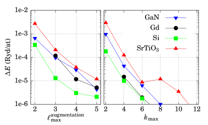
Figure 11: Convergence of the total energy with respect to augmentation $\ell$-cutoff and polynomial degree, Eq. (145).

This explains why the pseudopotential and PAW approximations can be truncated at much lower $\ell$ than the conventional augmented wave methods. Indeed, the present approach has much in common with PAW, but does not make approximations or involve pseudo-partial waves or projector functions.

3.7 Secular Matrix

To construct the secular matrix, we need matrix elements of Hamiltonian and overlap:

$$H_{ij}=\int\chi_{i}^{*}({{\mathbf{r}}})[-\nabla^{2}+V({{\mathbf{r}}})]\chi_{j}({{\mathbf{r}}})\,d^{3}r$$

$$S_{ij}=\int\chi_{i}^{*}({{\mathbf{r}}})\chi_{j}({{\mathbf{r}}})\,d^{3}r$$

At this stage we need not specify what $\chi_{i}$ is, except to note that it has an envelope part $\chi_{i}^{(0)}$ that extends everywhere in space, augmented in spheres taking the form Eq. (143). Specifically

$${\chi}_{i}({{\mathbf{r}}})=\chi^{0}_{i}({{\mathbf{r}}})+\sum_{kL}C^{(i)}_{kL}\Bigl{\{}\tilde{P}_{kL}({{\mathbf{r}}})-P_{kL}({{\mathbf{r}}})\Bigr{\}}$$ (145)

where $C^{(i)}_{kL}$ are the coefficients (Eq. (142)) that expand the smooth envelope in $\chi$ as polynomials $P_{kL}({{\mathbf{r}}})$ (Eq. (133)) and

$$\tilde{P}_{kL}({{\mathbf{r}}}) =\Bigl{[}A_{kl}\phi_{\ell}(r)+B_{kl}\dot{\phi}_{\ell}(r)\Bigr{]}Y_{L}(\hat{r})$$

$$\equiv\tilde{p}_{kl}(r)Y_{L}(\hat{r})$$ (146)

$\phi_{\ell}(r)$ and $\dot{\phi}_{\ell}(r)$ are the linearised partial waves, Sec.2.4. Coefficients $A_{kl}$ and $B_{kl}$ are chosen so that $\tilde{p}_{kl}$ and $p_{kl}$ have the same value and slope at $s_{R}$.

3.7.1 Overlap and Kinetic Energy, and Output Density

We use Eq. (144) to construct matrix elements of augmented basis functions. Matrix elements of overlap and kinetic energy may be written

$$\int\chi^{*}_{i}[-\nabla^{2}]\chi_{j}\,d^{3}r=\int{\chi_{i}^{(0)}}^{*}[-\nabla^{2}]\chi_{j}^{(0)}\,d^{3}r\\ +\sum_{kk^{\prime}L}C^{(i)*}_{kL}\tau_{kk^{\prime}l}C^{(j)}_{k^{\prime}L}$$ (147)

$$\int\chi^{*}_{i}\chi_{j}\,d^{3}r=\int{\chi_{i}^{(0)}}^{*}\chi_{j}^{(0)}\,d^{3}r\\ +\sum_{kk^{\prime}L}C^{(i)*}_{kL}\sigma_{kk^{\prime}\ell}C^{(j)}_{k^{\prime}L}$$ (148)

where

$$\tau_{kk^{\prime}\ell}=\int_{S}\Bigl{\{}\tilde{P}_{kL}[-\nabla^{2}]\tilde{P}_{k^{\prime}L}-P_{kL}[-\nabla^{2}]P_{k^{\prime}L}\Bigr{\}}\,d^{3}r$$ (149)

$$\sigma_{kk^{\prime}\ell}=\int_{s_{R}}\Bigl{\{}\tilde{P}_{kL}\tilde{P}_{k^{\prime}L}-P_{kL}P_{k^{\prime}L}\Bigr{\}}\,d^{3}r$$ (150)

The local kinetic energy matrix $\tau_{kk^{\prime}l}$ is symmetric, even while the individual terms in Eq. (149) are not, because the integral is confined to a sphere. However the surface terms from the true and smooth parts cancel because $\tilde{P}_{kL}$ and $P_{kL}$ match in value and slope there.

Note also that if $\phi_{\ell}$ and $\dot{\phi}_{\ell}$ are kept frozen, e.g. computed from a free atom as we might do to mimic a PAW or a pseudopotential method, $\tau_{kk^{\prime}\ell}$ and $\sigma_{kk^{\prime}\ell}$ are independent of environment. Though we won’t pursue it here, it suggests a path to constructing a unique and transferable pseudopotential.

Matrix elements of the potential are more complicated and will be discussed in the next section. For now we take them as given, along with the overlap and kinetic energy. We can diagonalise the secular matrix and obtain eigenfunctions and the output density as a bi-linear combination of basis functions

$$\psi_{n}({{\mathbf{r}}}) =\sum_{i}Z_{in}{\chi}_{i}({{\mathbf{r}}})$$

$$n^{\text{out}}({{\mathbf{r}}}) =\sum_{n}w_{n}\left|\psi_{n}({{\mathbf{r}}})\right|^{2}$$

$$=\sum_{ij}\Bigl{\{}\sum_{n}w_{n}Z^{*}_{in}Z_{jn}\Bigr{\}}\chi^{*}_{i}({{\mathbf{r}}})\chi_{j}({{\mathbf{r}}})$$ (151)

where the sum runs over the occupied eigenstates with $w_{n}$ the occupation probability. The bi-linear product may be written in a three-component form

$${\chi_{i}}^{*}{\chi}_{j}={\chi_{i}^{0}}^{*}\chi^{0}_{j}$$

$$+\sum_{Rkk^{\prime}LL^{\prime}}C^{(i)*}_{RkL}\Bigl{\{}\tilde{P}_{RkL}\tilde{P}_{Rk^{\prime}L^{\prime}}-P_{RkL}P_{Rk^{\prime}L^{\prime}}\Bigr{\}}C^{(j)}_{Rk^{\prime}L^{\prime}}$$ (152)

The first term yields a smooth $n_{0}$ which extends everywhere, and then two local terms, true and one-centre expansion of $n_{0}$ to some $L$ cutoff

$$n^{\text{val}}({{\mathbf{r}}})=n^{\text{val}}_{0}({{\mathbf{r}}})+\sum_{RL}\Bigl{\{}n^{\text{val}}_{1RL}({{\mathbf{r}}})-n^{\text{val}}_{2RL}({{\mathbf{r}}})\Bigr{\}}$$ (153)

As pointed out before, we expect the higher $L$ components be carried accurately by $n^{\text{val}}_{0}$ even for low $\ell_{\text{max}}$, which provides a simple justification for the pseudopotential and PAW approximations.

3.7.2 Core

The core levels and core density can be computed either scalar-relativistically or fully relativistically from the Dirac equation (Sec. 2.17). The core density is constructed in one of two ways: Self-consistent core: a core partial wave $\phi^{c}_{\ell}$ is integrated in the true potential, subject to the boundary condition $\phi_{c}(s_{R})=\phi^{\prime}_{c}(s_{R})=0$. It was once thought that the advantage of determining the core in the true potential outweighed the inaccuracy originating from the artificial boundary condition at $s_{R}$. Frozen overlapping core approximation: $\phi^{c}_{\ell}$ is computed in the free atom and kept frozen—experience shows this to be a better approximation. We develop this case here.

The core density has three components, which add to the valence density:

$$\tilde{n}_{0}({{\mathbf{r}}}) =\tilde{n}^{\text{val}}_{0}({{\mathbf{r}}})+\sum_{R}g^{\text{cn}}_{R}({{\mathbf{r}}})$$

$$n_{1R}({{\mathbf{r}}}) =n^{\text{val}}_{1R}({{\mathbf{r}}})+n^{\text{core+nuc}}_{1R}({{\mathbf{r}}})$$

$$\tilde{n}_{2R}({{\mathbf{r}}}) =\tilde{n}^{\text{val}}_{2R}({{\mathbf{r}}})+g^{\text{cn}}_{R}({{\mathbf{r}}})$$ (154)

where

$$g^{\text{cn}}_{R}({{\mathbf{r}}})=C^{G}\,G_{L{=}0}(r_{g};{{\mathbf{r}}})+C^{H}\mathcal{H}_{L{=}0}(E_{c};r_{h};{{\mathbf{r}}})$$ (155)

The second term is a smooth Hankel function with $C^{H}$ fixed to fit the spill-out of the core density into the interstitial. It is important that this be taken into account when constructing the total energy and potential. The alternative, to renormalise the core and confine it to the sphere, is a much cruder approximation. This makes it possible for shallow cores to be treated accurately, without needing to include them in the secular matrix (unfortunately at the loss of strict orthogonality between these and the valence states).

The pseudocores $g^{\text{cn}}_{R}$ in $\tilde{n}_{0}$ and $\tilde{n}_{2R}$ nearly cancel, but they need to be included to construct $V^{\text{eff}}$ and the total energy described below. Also the two kinds of $g^{\text{cn}}_{R}$ do not exactly cancel because it extends into the interstitial in the former case, but is truncated in the latter.

Smoothing radius $r_{g}$ must be small, so the core density is almost completely confined to the sphere. In practice we use the same Gaussians as for $g^{\text{val}}_{R}$ entering into the valence multipole moments (see Eq. (156) below). In that way $g^{\text{cn}}_{R}$ and $g^{\text{val}}_{R}$ can be merged together. The Hankel smoothing radius $r_{h}$ is chosen independently, but it is also typically small, of order $s_{R}/2$. The result should depend minimally on the choice of either.

3.7.3 Local Orbitals

Inside augmentation spheres, the usual Hilbert space consists of partial waves $\{\phi_{\ell},\,\dot{\phi}_{\ell}\}$. Questaal has the ability to extend this space by one local orbital (LO), to $\{\phi_{\ell}(\varepsilon_{\nu},r),\,\dot{\phi}_{\ell}(\varepsilon_{\nu},r),\,\phi^{z}_{\ell}(\varepsilon_{z},r)\}$. $\phi^{z}_{\ell}$ consists of a partial wave evaluated at some energy $\varepsilon_{z}$ far above or far below the linearisation energy $\varepsilon_{\nu}$ for $\phi_{\ell}$. Addition of a LO greatly extends the energy window over which the band structure is valid; see for example Fig. 1, of Ref. [56], where the band structure for Si was compared to LAPW, and to a full (non-linearised) APW. Properties of Questaal’s LO are explained in that reference in a GW context; here we outline the main features.

LO have one each of the following attributes:

• either core-like or high in energy, with principal quantum number $\mp$ 1 that of valence $\phi_{\ell}$, respectively;

• either a conventional LO, which consists $\phi_{z}$ with some $\phi_{\ell}$ and $\dot{\phi}_{\ell}$ admixed to make the value and slope vanish at $s_{R}$ [57], or an extended LO, which consists of $\phi_{z}$ with a smooth Hankel function tail that extends continuously and differentiably into the interstitial. The extended LO can be applied only to the core-like case; and

• either a scalar relativistic LO, or a Dirac LO with $\mu{=}1/2$. This is not usually important, but it can have consequences for heavy elements; see how it affects LDA and GW gaps in Sec. 3.9. This method was first introduced by Kunes̆ et al.[58].

High-lying states are not usually important for DFT, because states above $E_{F}$ do not contribute to the potential. Core states of order $E_{F}{-}2$ Ry and deeper can usually be treated quite adequately as core levels integrated independently of the secular matrix (Sec. 3.7.2). There are mild exceptions: for high resolution such as needed for the Delta Codes project (Sec. 3.13), both deep and high-lying LO were used (in the latter case, particularly adding $4d$ LO to the $3d$ transition metals).

GW is more sensitive to states far from $E_{F}$ than DFT. Including low-lying cores at $E_{F}{-}2$ Ry or even somewhat deeper with LO can modify valence QP levels by $\sim$0.1 eV. High-lying states are also more important in the GW context. ZnO is an extreme case where they were found to shift the gap by several tenths of an eV [59], and many high-lying LOs are required to reach convergence[60].

3.7.4 Effective Potential

We seek a three-component form of the total energy functional. Its variational derivative with respect to the density yields an effective potential $V^{\text{eff}}$, which should give the first-order variation of the electrostatic and exchange-correlation energy with respect to the trial density. The density has three components, the first interacts with a smooth potential $\tilde{V}_{0}$, the second with the local true potential $V_{1R}$, and the third with the local projection of the potential $V_{2R}$. Correspondingly, the accumulated sums over the first, second, and third terms produce $n^{\rm out}_{0}$, $n^{\rm out}_{1R}$, and $n^{\rm out}_{2R}$, respectively.

Construction of $V^{\text{eff}}$ is complicated by the fact that the electrostatic potential at some point depends on the density everywhere. Therefore it is not possible to construct the potential in a sphere solely from the density inside this sphere, or the smooth potential from $n^{\text{val}}_{0}$ alone. We can solve this difficulty by defining a pseudodensity $\tilde{n^{\text{val}}}_{0}$ which has the same multipole moments inside augmentation sphere $R$ as the true density ${n^{\text{val}}}_{1R}$. Suppose the local sphere density $n^{\text{val}}_{1R}-n^{\text{val}}_{2R}$ has multipole moments $q_{M}$, where $M$ = angular momentum. Then define

$$\tilde{n}^{\text{val}}_{0}({{\mathbf{r}}})=n^{\text{val}}_{0}({{\mathbf{r}}})+\sum_{R}g^{\text{val}}_{R}({{\mathbf{r}}})$$

$$g^{\text{val}}_{R}({{\mathbf{r}}})=\sum_{M}q_{RM}G_{RM}({{\mathbf{r}}})$$ (156)

where $G_{RM}$ is a Gaussian of angular momentum $M$ centred at $R$, with unit moment. $G_{M}$ must be sufficiently localised inside $s_{R}$ that the potential from the second term at $s_{R}$ is negligibly different from the potential of a unit point multipole at $R$ (typically $s_{R}/4$). Results should not depend on $r_{g}$, but in practice if it is made too small, numerical integration of the $G$ become inaccurate, while if too large charge is not confined to $s_{R}$. Provided it is confined, the compensating Gaussians ensure that the electrostatic potential $V^{\text{es}}[\tilde{n}^{\text{val}}_{0}]$ is exact in the interstitial.

The local representation $n^{\text{val}}_{2R}$ of the smoothed density must be equally compensated

$$\tilde{n}^{\text{val}}_{2R} =n^{\text{val}}_{2R}+g^{\text{val}}_{R}$$ (157)

The $q_{RM}$ can be decomposed into a sum of partial moments

$$q_{RM}=\sum_{kk^{\prime}LL^{\prime}}Q_{Rkk^{\prime}LL^{\prime}M}$$

$$Q_{Rkk^{\prime}LL^{\prime}M}=\int_{s_{R}}\Bigl{\{}\tilde{P}_{kL}\tilde{P}_{k^{\prime}L^{\prime}}-P_{kL}P_{k^{\prime}L^{\prime}}\Bigr{\}}\\ \times r^{m}Y_{M}(\hat{r})\,d^{3}r$$ (158)

By decomposing $q_{RM}$ this way, we can make any possible variation in the local density in the Hilbert space spanned by Eq. (152), and obtain the potential from the electrostatic corresponding to the variation.

Matrix elements of the local potential are determined from variation of the electrostatic energy (Sec. 3)

$$\pi_{1Rkk^{\prime}LL^{\prime}}= \int_{s_{R}}\tilde{P}_{RkL}V_{1R}\tilde{P}_{Rk^{\prime}L^{\prime}}\,d^{3}r$$

$$\pi_{2Rkk^{\prime}LL^{\prime}}= \int_{s_{R}}P_{RkL}\tilde{V}_{2R}P_{Rk^{\prime}L^{\prime}}\,d^{3}r$$

$$+\sum_{RM}Q_{Rkk^{\prime}LL^{\prime}M}\int_{s_{R}}\tilde{V}_{2R}G_{RM}\,d^{3}r$$ (159)

The true potential $V_{1R}$ is the response to true partial density $\tilde{P}_{RkL}\tilde{P}_{Rk^{\prime}L^{\prime}}$, and $\tilde{V}_{2R}$ the response to the smooth partial density $P_{RkL}P_{Rk^{\prime}L^{\prime}}+\sum Q_{Rkk^{\prime}LL^{\prime}M}G_{RM}$. These two partial densities have the same multipole moments by construction.

We solve the Poisson equation for each of the three components

$$\nabla^{2}\tilde{V}^{\rm es}_{0} =-8\pi\tilde{n}_{0}$$

$$\nabla^{2}V^{\rm es}_{1R} =-8\pi n_{1R}$$

$$\nabla^{2}\tilde{V}^{\rm es}_{2R} =-8\pi\Bigl{\{}n_{2R}+\sum\nolimits_{M}q_{RM}G_{RM}\Bigr{\}}$$ (160)

All density components must include core (or pseudocore) contributions (Sec. 3.7.2). Poisson’s equation for $\tilde{V}^{\rm es}_{0}$ is most easily solved by fast Fourier transforming $\tilde{n}_{0}$ to reciprocal space, scaling each Fourier component $n_{G}$ by $-8\pi/G^{2}$ and transforming back. In principle the electrostatic potential can be calculated this way but in practice the compensation Gaussians in $\tilde{n}_{0}$ can be fairly sharply peaked. Some parts are separated out and evaluated analytically to keep the plane wave cutoff low, as discussed in the next section. $\tilde{V}^{\text{es}}_{0}({{\mathbf{r}}})$ is exact in the interstitial region and extends smoothly through the spheres. $V^{\rm es}_{1R}$ and $\tilde{V}^{\rm es}_{2R}$ can be solved up to an arbitrary homogeneous solution which is determined by the boundary condition at $s_{R}$. This adds a term proportional to $r^{m}Y_{M}({{\mathbf{r}}})$, which is determined by resolving $\tilde{V}^{\rm es}_{0}$ into a one-centre expansion at $s_{R}$.

Pseudopotentials $\tilde{V}^{\rm es}_{0}$ and $\tilde{V}^{\rm es}_{2R}$ approximately cancel each other, but not exactly. This is in part because the latter has a finite $L$ cutoff, and in part because $\tilde{V}^{\rm es}_{0}$ carries the tails of the core densities spilling into the interstitial. These incomplete cancellations are the key to rapid $\ell$ convergence of this method, and also allow relatively shallow cores not to be included in the secular matrix, with minimal loss in accuracy.

Three Component Total Energy in DFT

The total energy in DFT is comprised of the kinetic energy, electrostatic energy, and exchange-correlation energy

$$E_{\text{tot}}=\left<T\right>+U+E_{\text{xc}}$$ (161)

Questaal implements two functionals for $E_{\text{tot}}$. The traditional Kohn-Sham functional is evaluated at the output density: $U$ and $E_{\text{xc}}$ are evaluated from $n_{\text{out}}$ generated by the secular matrix, and $\left<T\right>_{\text{HKS}}=\sum_{i}^{\text{occ}}\left<\psi_{i}|-\nabla^{2}|\psi_{i}\right>+T_{\text{core}}$. ${T}_{\text{core}}=\sum\epsilon_{i}^{\rm core}-\int n^{\rm core}V^{\text{eff}}$ is the kinetic energy of the core. If the core is kept frozen, it can be evaluated from the free atom.

Harris [61] and independently Foulkes and Haydock [62] showed that the kinetic energy can be expressed in terms of $n_{\text{in}}$: $U{=}U[n_{\text{in}}]$ and $E_{\text{xc}}{=}E_{\text{xc}}[n_{\text{in}}]$ and

$$\left<T\right>_{\text{HF}}=\sum_{i}^{\text{occ}}\epsilon_{i}^{\text{val}}-\int n_{\text{in}}^{\text{val}}V_{\text{in}}^{\text{eff}}+T_{\text{core}}$$ (162)

Both $E_{\text{HKS}}$ and $E_{\text{HF}}$ are calculated, though usually the latter is preferred because it converges more rapidly with deviations from self-consistency. It is nevertheless useful to have both energies, because they are calculated differently in Questaal. $U$ and $E_{\text{xc}}$ are computed from different densities, but more, $\left<T\right>_{\text{HKS}}$ and $\left<T\right>_{\text{HF}}$ are calculated in different ways. It is not trivial that at (nominal) self-consistency $E_{\text{HKS}}{=}E_{\text{HF}}$. The two always differ slightly; when they differ more than a small amount, it is an indication that some parameter (e.g. plane-wave cutoff) is set too low. Thus, $E_{\text{HKS}}{-}E_{\text{HF}}$ is one measure of the convergence of the basis representing the charge density.

In Questaal’s three-component framework, $nV^{\text{eff}}$ a sum of three terms bilinear in the three components $\tilde{n}_{0}\tilde{V}^{\rm es}_{0}$, $n_{1R}V^{\rm es}_{1R}$ and $\tilde{n}_{2R}\tilde{V}^{\rm es}_{2R}$. $\left<T\right>$, $U$ and $E_{\text{xc}}$ each have independent contributions from three components, for example the contribution to the electrostatic energy from the valence electrons is

$$E^{\text{es}}=\frac{1}{2}\int\tilde{n}_{0}^{\text{val}}({{\mathbf{r}}})\tilde{V}_{0}^{\text{es}}({{\mathbf{r}}})\\ +\sum_{R}\int_{S_{R}}\Bigl{\{}n^{\text{val}}_{1R}V^{\rm es}_{1R}\,d^{3}r-\tilde{n}^{\text{val}}_{2R}\tilde{V}^{\rm es}_{2R}\Bigr{\}}\,d^{3}r$$ (163)

The last term cancels most of the first inside the augmentation spheres, except the first retains $L$ components above $\ell_{\text{max}}$ to all orders. This is because $\tilde{V}_{2R}$ should be a one-centre expansion of $\tilde{V}_{0}$ up to $\ell_{\text{max}}$, and $\tilde{n}^{\text{val}}_{2R}$ should be a one-centre expansion of $\tilde{n}^{\text{val}}_{0}$. Because $V^{\text{es}}[\tilde{n}^{\text{val}}_{0}]$ is exact in the interstitial, including at $s_{R}$, and it continued inside $s_{R}$ by adding by $V^{\rm es}_{1R}\,d^{3}r-\tilde{V}^{\rm es}_{2R}$, the true potential is correct everywhere. Note that the derivative of $E^{\text{es}}$ wrt coefficients $C^{(i)}_{Rk^{\prime}L^{\prime}}$ in Eq. (152) yield the local potentials Eq. (159), so that the effective one-body Hamiltonian corresponds to the functional derivative of the energy.

The total electrostatic energy must include the core. Write it analogously to Eq. (163) but add the (pseudo) core and nuclear density to $n^{\text{val}}$ (Sec. 3.7.2)

$$U=\tilde{U}_{0}+\sum_{R}\{U_{R}-\tilde{U}_{R}\}$$ (164)

The first term is the electrostatic energy of the smooth density, evaluated on a uniform mesh. It involves a valence and pseudo-(core+nucleus) term

$$\tilde{U}_{0}=\tilde{U}_{0}^{\text{val}}+\tilde{U}_{0}^{\text{c+n}}$$

$$\tilde{U}_{0}^{\text{val}}=\frac{1}{2}\int\,d^{3}r\,\tilde{n}_{0}^{\text{val}}({{\mathbf{r}}})\,\tilde{V}^{\text{es}}({{\mathbf{r}}})$$

$$\tilde{U}_{0}^{\text{c+n}}=\sum_{R}(C^{G}_{R}-Z_{R})V^{G}_{R0}+C^{H}_{R}V^{H}_{R}$$

where

$$V^{G}_{RL} =\int\,d^{3}r\,G_{RL}\tilde{V}^{\text{es}}[\tilde{n}_{0}]$$

$$V^{H}_{R} =\int\,d^{3}r\,\mathcal{H}_{R0}\tilde{V}^{\text{es}}[\tilde{n}_{0}]$$

Besides being needed for ${U}_{0}^{\text{c+n}}$, $V^{G}_{RL}$ is used in assembling $\tilde{U}_{0}^{\text{val}}$. $\tilde{U}_{0}^{\text{c+n}}$ and $\tilde{U}_{0}^{\text{val}}$ must be evaluated with some care to avoid numerically integrating sharply peaked functions (core pseudodensity and the multipole contribution to $\tilde{n}_{0}$ (Eq. (156)). $V^{G}_{RL}$ and $V^{H}_{R}$ are evaluated by splitting the potential into two terms $\tilde{V}^{\text{es}}[\tilde{n}_{0}]=\tilde{V}^{\text{es}}[{n}_{0}]+\{\tilde{V}^{\text{es}}[\tilde{n}_{0}]-\tilde{V}^{\text{es}}[{n}_{0}]\}$. Integrals of the second term can be performed analytically (the interested reader is referred to Section XI of Ref. [31]), thus avoiding integrals of sharply peaked functions. All of the other integrals are much smoother and are evaluated on the grid of $G$ vectors.

$U_{R}$ and $\tilde{U}_{R}$ are readily integrated in the sphere together with the valence parts in Eq. (163).

The exchange-correlation potential is made analogously with the electrostatic potential:

$$E {}_{xc}=\int n_{0}\epsilon_{\rm xc}[n_{0}]\,d^{3}r$$

$$+\sum_{R}\int_{s_{R}}\Bigl{\{}n_{1R}\epsilon_{\rm xc}[n_{1R}]-n_{2R}\epsilon_{\rm xc}[n_{2R}]\Bigr{\}}\,d^{3}r$$ (165)

It is also divided into valence + core contributions.

We reiterate that differences $\int n_{1R}V^{\rm es}_{1R}\,d^{3}r-\tilde{n}_{2R}\tilde{V}^{\rm es}_{2R}$ and $\int n_{1R}\epsilon_{\rm xc}(n_{1R})-n_{2R}\epsilon_{\rm xc}(n_{2R})$ converge much more rapidly with $\ell$-cutoff than either term separately, and as a consequence the three-component augmentation is much more efficient than the standard one.

3.7.5 Forces

Our original formulation [31] derived a simple expression for the derivative of $H_{\text{HF}}$ when a nucleus changes from ${{\mathbf{R}}}$ to ${{\mathbf{R}}}{+}\delta{{\mathbf{R}}}$, assuming that the partial waves $\phi_{R\ell}$ shift rigidly with $\delta{{\mathbf{R}}}$. (lmf has a “frozen $\phi$” switch, which if imposed, guarantees $\phi_{R\ell}$ is rigid. In practice we have found that the differences are small.)

The original expression yielded forces that converge only linearly with deviations ${\Delta}n{=}n_{\text{out}}{-}n_{\text{in}}$ from self-consistency. It is possible to achieve faster convergence in ${\Delta}n$, by adding a correction ${\delta}V{\Delta}n$, where ${\delta}V$ is determined from a change ${\delta{n}_{\text{in}}}$ in $n_{\text{in}}$, but there is no unambiguous way to determine ${\delta{n}_{\text{in}}}$. If the static susceptibility (Sec. 6) were calculated, a good estimate could be made. But $\chi({{\mathbf{r}}},{{\mathbf{r}}}^{\prime},0)$ is a second derivative of $H_{\text{HF}}$: it is far more cumbersome to make than $H_{\text{HF}}$ itself, and approximation of $\chi$ by models such as the Lindhard function worked less well than hoped. A practicable, and simple alternate ansatz is to assume that ${\delta{n}_{\text{in}}}$ is given by a change in the Mattheis density construction (superposition of free-atomic densities), arising ${\delta}{{\mathbf{R}}}$. This has worked very well in practice: it dramatically improves the convergence of the forces with iterations to self-consistency. Here we omit the derivation but refer to the original paper [31], and also to Appendix B of Ref. [52] for an alternate derivation including the correction term. The final expression for shift of nucleus $R$ from ${{\mathbf{R}}}{\to}{{\mathbf{R}}}{+}\delta{{\mathbf{R}}}$ is

$$\delta E_{\rm H}=\int\tilde{V}_{0}\,\delta{g^{\text{cn}}_{R}}+\delta^{\rm R}\sum_{i}^{\text{occ}}\epsilon_{i}^{\text{val}}+{\delta}V_{\text{in}}(n_{\text{out}}{-}n_{\text{in}})$$ (166)

$\tilde{V}_{0}$ is the sum of the smooth electrostatic and exchange-correlation potential. This term describes the force of the smooth density on the Gaussian lumps which represent the core and the nucleus at each site, and is the analogue of the Hellmann-Feynman theorem.

The eigenvalue shifts account for a change in the atom-centred basis set in the shift in ${{\mathbf{R}}}$. This the price for taking a tailored basis, but one whose Hilbert space changes when ${{\mathbf{R}}}$ shifts. Here the smooth mesh potential is fixed and augmentation matrices $\tau$, $\sigma$, and $\pi$ (Eqs. (149), (150) and  (159)) shift rigidly with the nucleus. Gradients only include redistribution of plane waves owing to the shifts in envelope functions, and in the expansion coefficients $C^{(j)}_{Rk^{\prime}L^{\prime}}$ (Eq. (145)).

The last term is the correction noted above. In future, it will probably be replaced by an efficient calculation of $\chi$; meanwhile the Mattheis-shift ansatz works rather well. Fig. 12 shows the force $F_{\text{Ox}}$ on an O neighbouring Co substituted for Ti in a 12-atom unit cell of TiO₂, as lmf iterates to self-consistency. The deviation ${\Delta}F$ from the self-consistent force is vastly smaller with the correction term (compare solid and dashed lines), and $F_{\text{Ox}}$ is reasonable already for the Mattheis construction (first iteration). The inset compares the two kinds of ${\Delta}F$ with iteration to self-consistency to show that without and with the correction, ${\Delta}F$ scales as ${\Delta}F^{\mathrm{uncorr}}_{\mathrm{Ox}}{\sim}\overline{\Delta\mathrm{Q}}$ and ${\Delta}F^{\mathrm{corr}}_{\mathrm{Ox}}{\sim}(\overline{\Delta\mathrm{Q}})^{2}$, the latter being the same rate of convergence as the energy itself.

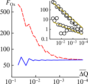
Figure 12: Harris force $F_{\text{Ox}}$ (mRy/au) on O neighbouring Co in Co-doped TiO₂. $\overline{\Delta\mathrm{Q}}$ is a measure of the RMS change $n_{\text{out}}{-}n_{\text{in}}$ integrated over the unit cell. Solid and dashed lines are Eq. (166) with and without the third term. Inset shows deviation in $F_{\text{Ox}}$ from the converged value. Yellow lines show $\overline{\Delta\mathrm{Q}}$ and $(\overline{\Delta\mathrm{Q}})^{2}$ as guides to the eye.

3.8 LDA+U

The LDA+U method, introduced originally by Anisimov et al. [63, 64, 65] for open shell $d$- or $f$-shell materials including on-site Coulomb and exchange interactions by means of the Hubbard model is implemented in both the lm and the lmf codes following the rotationally invariant approach described in [66]. Rotational invariance means that the occupations of the different $d_{m}$ orbitals are specified by a density matrix ${\bf n}^{\sigma}=n_{mm^{\prime}}^{\sigma}$ independent of the specific choice of Cartesian axes defining the spherical harmonics. For brevity we refer to the orbitals on which $U$ is applied as the $d$ orbitals although the code is written sufficiently general that $U$ terms can be applied to any $nl$ of choice and even on multiple sets of orbitals.

The on-site Coulomb interactions are added to the LSDA total energy and a double-counting term is subtracted.

$$E^{LDA+U}[\rho^{\sigma}({{{\mathbf{r}}}}),{\bf n}^{\sigma}]=E^{LSDA}[\rho^{\sigma}({\bf r})]+E^{U}[{\bf n}^{\sigma}]\\ -E_{dc}[{\bf n}^{\sigma}]$$ (167)

Several schemes for the double counting have been proposed [63, 64, 66, 67, 68] and are implemented in lmf but the prevailing approach is the fully localised limit (FLL) in which the double-counting term and $U$-terms cancel for the fully localised (atomic) limit in which the density matrix becomes a diagonal matrix with integer occupations. This means that in principle the total energy is already well described in the LSDA in the atomic limit but the orbital energies are not. The task of the LSDA+U approach is to optimise the density matrix when the orbitals on which $U$ is applied are allowed to hybridise with the other orbitals in the system. It hence describes strictly speaking the orbital polarisation in the system. Note that the total energy is then separately a functional of the spin-dependent electron density and the local density matrix on the orbitals for which $U$ terms are added. The density matrix or orbital occupations also influence the spin-charge densities and so the two contributions are not really independent. The $U$ terms in LSDA+U are treated in the static mean-field Hartree-Fock approximation in contrast to the DMFT method where they are treated dynamically. The expressions for the $E^{U}[{\bf n}^{\sigma}]$ part of the total energy can be found in [66] and are given in terms of density matrices $n^{\sigma}_{mm^{\prime}}$ and matrix elements of the Coulomb interaction $\langle m,m^{\prime\prime}|V_{ee}|m^{\prime},m^{\prime\prime\prime}\rangle$. They fully take into account the rotational aspects of the $Y_{lm}$ of the $d$-states included. The double counting term, on the other hand, is written in terms of average Coulomb $U$ and exchange $J$ parameters and involves only the the trace of the density matrix $n^{\sigma}=Tr({\bf n}^{\sigma})$.[66] $U$ and $J$ are the screened Coulomb and exchange parameters, which can for example, be estimated by a separate self-consistent supercell calculation treating the atoms in which the $d$-orbital occupation is changed as an impurity problem [69]. or by means of the linear response approach [70]. Most often they are treated empirically and $U$ is adjusted to spectroscopic splittings, for example.

The bare Coulomb interaction matrix elements can be evaluated exactly in terms of the Slater $F^{k}(ll)$ integrals and combinations of Gaunt coefficients as worked out for instance in Condon and Shortley [71]. The Slater $F^{k}(ll)$-integrals,

$$F^{k}(ll)=\int\int r_{1}^{2}dr_{1}r_{2}^{2}dr_{2}R_{\ell}(r_{1})^{2}R_{\ell}(r_{2})^{2}(r_{<}^{k}/r_{>}^{k+1})$$ (168)

where $r_{<}$, $r_{>}$ are the smaller and larger or $r_{1}$ and $r_{2}$ could easily be calculated directly in terms of the partial waves inside the spheres. However, this would then not take into account the screening of the Coulomb interaction by the other orbitals in the system. Therefore it is customary to use the relation between the average $U$ and $J$ to the $U_{mm^{\prime}}$ and $J_{mm^{\prime}}$

$$U=\frac{1}{(2\ell+1)^{2}}\sum_{mm^{\prime}}U_{mm^{\prime}}=F^{0}$$

$$U-J=\frac{1}{2\ell(2\ell+1)}\sum_{mm^{\prime}}(U_{mm^{\prime}}-J_{mm^{\prime}})$$ (169)

given by Anisimov et al. [64] and where $U_{mm^{\prime}}=\langle mm^{\prime}|V_{ee}|mm^{\prime}\rangle$, $J_{mm^{\prime}}=\langle mm^{\prime}|V_{ee}|m^{\prime}m\rangle$. Using the tables of Condon and Shortley [71] one finds for $d$ electrons

$$14J=F^{2}(dd)+F^{4}(dd)$$ (170)

and for $f$ electrons

$$3J=\frac{2}{15}F^{2}(ff)+\frac{1}{11}F^{4}(ff)+\frac{1}{858}F^{6}(ff)$$ (171)

For $p$-orbitals $J=F^{2}(pp)/5$ and for $s$-orbitals $J=0$. Examining the tabulated values of the Slater $F^{k}$ integrals from Hartree-Fock calculations, one finds that the ratios $F^{4}(dd)/F^{2}(dd)\approx 0.625$ and $F^{6}(ff)/F^{2}(ff)\approx 0.494$, $F^{4}(ff)/F^{2}(ff)\approx 0.668$ are approximately constant. Using these fixed ratios and the relation to the average exchange integral $J$ one then can fix the $F^{k}$ values. The advantage of doing it this way is that the screening of the $J$ and $U$ can then be taken into account and there are only two empirical parameters. On the other hand one finds in practice that while $U$ is strongly reduced from the atomic bare $F^{0}$, the $J$ is approximately unscreened, so one might as well use the unscreened directly calculated $F^{k}$ for $k\geq 2$. From LDA calculated atomic wave functions, we find $F^{4}(dd)/F^{2}(dd)=0.658\pm 0.004$ for $3d$ atoms, $F^{4}(ff)/F^{2}(Ff)=0.685\pm 0.001$, $F^{6}(ff)/F^{2}(ff)=0.518\pm 0.001$ for rare-earth RE³⁺. (Until recently, Questaal used a different convention; see note [72].)

By minimising the LDA+U total energy with respect to the density matrix elements, one obtains a non-local potential $V^{\sigma}_{mm^{\prime}}$ which can also be found in [66]. In the ASA lm-version it is straightforward to add this nonlocal potential directly to the Hamiltonian inside the spheres because the orbitals defining the matrix $V^{\sigma}_{mm^{\prime}}$ are just the single $lm$ channel partial waves inside the sphere. It is a little more complex in lmf. Essentially, we now add the operator $|\phi^{\sigma}_{lm}\rangle V^{\sigma}_{mm^{\prime}}\langle\phi^{\sigma}_{lm^{\prime}}|$. We add the corresponding augmentation matrix elements both for the $\phi$ and $\dot{\phi}$ and for local orbitals if these are present for this $\ell$ channel.

The calculation within LDA+U starts from a set of initial occupation numbers of the $m$ orbitals for each channel $\ell$ for which $U$ and $J$ parameters are provided. These define the initial density matrix. The calculation then proceeds by making this density matrix self-consistent simultaneously with making the standard spin density $\rho^{\sigma}({\bf r})$ self-consistent. We note that the configuration one converges to may depend on the starting density matrix and hence one should in principle consider different starting points and find the one which minimises the energy or use guidance from physical insight. In rare-earth (RE) based systems one finds for example that the lowest energy corresponds to the configuration which obeys Hund’s rules [73].

We have here described only the FLL. The around-mean-field approach [67, 63] and a mixture of the two [68] are also implemented and make use of the same ingredients. Recently, Keshavarz et al. [74] argued that adding $U$ to spin-unpolarised LDA, thus LDA+U may have advantages over adding them to LSDA, for example to extract inter-atomic exchange interactions independent of the reference system used (AFM or FM). This is presently not supported in the lm and lmf codes but might be useful to add in the future. Note that in Ref. [64] also a LDA+U rather LSDA+U approach was used.

A simpler version of the LDA+U is described by Dudarev et al. [75]. In that case, only a single parameter, namely $\tilde{U}=U-J$ comes into play. One can use this scheme in the codes by setting $J=0$ and adjusting the provided $\tilde{U}$ parameter. This means essentially that we neglect the orbital polarisation due to the anisotropic Coulomb interaction exchange terms but keep the Hartree-Fock like feature that empty states feel a different potential from occupied states. In fact, in this case the additional potential is

$$V^{\sigma}_{mm^{\prime}}=\tilde{U}[{\scriptstyle\frac{1}{2}}\delta_{mm^{\prime}}-n^{\sigma}_{mm^{\prime}}]$$ (172)

Or if the density matrix is actually diagonal $V^{\sigma}_{m}=\tilde{U}[{\scriptstyle\frac{1}{2}}-n^{\sigma}_{m}]$. This means that when a spin-orbital $m\sigma$ on a given site is empty it is shifted up by $\tilde{U}/2$ and when it is filled, it is shifted down by $\tilde{U}/2$. This corresponds to the simplest form of the LDA+U formalism. It allows one for example to include a shift of a fully occupied $d$ band. This is useful for example in Zn-containing systems. In LDA, the binding energy of these orbitals is underestimated. The deeper a band lies below the Fermi level, the higher its downward shift by the self-energy and this can be simply mimicked by the LDA+U method in this form. It has the effect for example of reducing the hybridisation of the Zn-$3d$ with the valence band maximum and slightly increases the gap, affects things like band-offsets and the valence band maximum crystal field and spin-orbit induced fine splitting.

One can even use this approach for $s$ or $p$ electrons and thereby shift up the mostly cation-$s$ like conduction band minimum in a semiconductor to adjust the gap. While this is of course purely empirical and shifting the gaps for the wrong reason, and hence far less accurate than the QSGW approach, it is sometimes useful in defect calculations because a defect level that would otherwise lie as a resonance in the conduction band can now become a defect level in the gap and allow one to properly control its occupation for different charge states of the defect. Using a $U$ on $p$-orbitals of anions like O or N, this can also have the effect that the empty defect levels pushed out the valence band and localising on a single $p$ orbital are pushed deeper into the gap. The essential function of the LDA+U terms in these applications is to introduce a Hartree-Fock like orbital dependence of the potential. This is important to reduce the self-interaction error of LDA or GGA and allows one in a simpler and much less expensive way to simulate what a hybrid functional would do. If one picks these shifts carefully to adjust the bulk band structure to the QSGW bands, it provides a rather efficient way to study defects with a corrected band gap and specific orbital self-interaction, two of the main errors of LDA plaguing defect calculations. An example of this can be found in Boonchun et al. [76].

3.9 Relativistic Effects

The radial solvers all solve by default a scalar Dirac equation, which incorporates the dominant relativistic effects. All the DFT codes (lmf, lm, lmgf and lmpg) have the ability to incorporate spin-orbit coupling perturbatively. In the band codes the perturbation is straightforward (See Sec. 2.8.2); the Green’s function scheme is more subtle, particularly with respect to third order parameterisation, but a formulation is possible (Sec. 2.16). For lmf, the ${\mathbf{L}}\cdot{\mathbf{S}}$ term is added to the true local potential $V_{1R}$ (see Sec. 3.7.4). As of this writing, only the spin diagonal part of the output density is kept in the self-consistency cycle.

Additionally the ASA codes lm, lmgf and lmpg have a fully relativistic implementation (Sec. 2.17). The full-potential code lmf does not as yet; however it does have a facility to compute the core levels fully relativistically. It follows a method similar to that developed by Ebert [42].

As of this writing, the QSGW code allows spin-orbit coupling only in a very restricted manner. Typically SOC has only a minor effect on the self-energy $\Sigma$: this is because SOC is a modification to the kinetic energy and only affects the potential in a higher order perturbation. We have found very good results by generating QSGW self-energies leaving out SOC all together, and then as a post-processing step include it in the band structure.

Additionally, lmf has a special mode where the only diagonal parts of ${\mathbf{L}}\cdot{\mathbf{S}}$ (see Sec. 2.8.2) are added to the one-particle Hamiltonian. After diagonalisation the spin off-diagonal parts are used to modify the one-particle levels in a special kind of perturbation theory, as described in the Appendix of Ref. [77]. This has the advantage that the eigenvectors are kept spin-diagonal, which significantly reduces the cost of the GW code. Tests show that at the LDA level the modification to the band structure is very similar to that of the full ${\mathbf{L}}\cdot{\mathbf{S}}$, and for purposes of determining the effect on $\Sigma$ it should be quite reliable except in very special cases. Once a modified $\Sigma$ has been found (as a one-shot correction to QSGW computed without SOC), lmf can be run with the full ${\mathbf{L}}\cdot{\mathbf{S}}$, including the modification of $\Sigma$ approximately in the manner just described. We have found the difference to be negligible except when elements are very heavy: CH₃NH₃PbI₃ is the most extreme case we have found so far: the effect of SO on the band structure through changes in $\Sigma$ reduced the gap by 0.1 eV [77]

Finally lmf has an ability to fold in approximately the effects of the proper Dirac Hamiltonian on the valence states. The difference between the full Dirac and scalar Dirac partial waves can be important for very small $r$, where the SOC contributions are the largest (see $\xi(r)$ in Sec. 2.8.2). For small ${{\mathbf{r}}}$, the true Dirac wave function varies as $r^{\gamma},\ \gamma^{2}={\kappa^{2}-(2Z/c)^{2}}$, whereas in the scalar Dirac case it varies as $r^{\ell}$. As a result, matrix elements $\xi(r)$ are underestimated. The effect is typically very small, but it becomes non-negligible in heavy semiconductors such as CdTe. To ameliorate this error, lmf has the ability to use a fully relativistic partial wave in place of a standard local orbital, choosing $\mu=-1/2$. Most important is the $p_{1/2}$ state with $\kappa=1$.

			LDA		QSGW
Material	${\begin{subarray}{c}n_{c}\\ n_{a}\end{subarray}}$	${\begin{subarray}{c}\gamma_{c}\\ \gamma_{a}\end{subarray}}$	$\Delta_{0}$	$E_{G}$	$\Delta_{0}$	$E_{G}$
GaAs (SR)	5	0.97	0.34	0.24	0.33	1.77
GaAs ($p_{1/2}$)	5	0.97	0.35	0.24	0.34	1.75
GaAs (expt)			0.34	1.52	0.34	1.52
ZnSe (SR)	5	0.98	0.39	0.95	0.39	3.05
ZnSe ($p_{1/2}$)	5	0.97	0.40	0.95	0.40	3.00
ZnSe (expt)			0.40	2.82	0.40	2.82
CdTe (SR)	6	0.94	0.84	0.26	0.83	1.83
CdTe ($p_{1/2}$)	6	0.93	0.92	0.26	0.88	1.77
CdTe (expt)			0.90	1.61	0.90	1.61
PbTe (SR)	7	0.80	1.12	-.16	1.00	0.40
PbTe ($p_{1/2}$)	6	0.93	1.30	-.57	1.06	0.22
PbTe (expt)				0.19		0.19

Table 4: Spin orbit splitting $\Delta_{0}$ of the valence band at $\Gamma$, and energy bandgaps computed in the LDA and by QSGW, with a scalar relativistic (SR) local orbital on the cation and anion $p$ states, and a Dirac $p_{1/2}$ local orbital. In the zincblende semiconductors the two band edges are at $\Gamma$, but in PbTe case they are both at L (Fig. 13). $n$ are the principal quantum numbers of the cation and anion local $p$ orbital; $\gamma=[1-(Z/c)^{2}]^{1/2}.$

SO coupling is well described for light semiconductors such as GaAs and ZnSe (see Table 4), as $Z$ increases $\gamma$ deviates progressively from unity and the discrepancy with experiment increases. It is already significant for CdTe, and in PbTe the effect exceeds 0.1 eV. Replacing the scalar Dirac LO with the Dirac $p_{1/2}$ LO significantly decreases this error in CdTe. In PbTe, the valence band edges are both at L: the two band edges have symmetry L${}_{6}^{+}$ and L${}_{6}^{-}$, respectively (Fig. 13). The LDA gap is nominally positive, but L${}_{6}^{+}$ and L${}_{6}^{-}$ are inverted very near L as can be seen by the change in colours at the band edges; thus the gap is actually inverted. Anticipating the discussion in Sec. 4, if a diagonal-only GW were carried out on top of this, the L${}_{6}^{+}$ and L${}_{6}^{-}$ would order properly, but the wrong topology would manifest itself as a band crossing near L, as shown for Ge in Fig. 6 of Ref. [56]. QSGW orders L${}_{6}^{+}$ and L${}_{6}^{-}$ correctly, somewhat overestimating the gap [78]. Adding a Dirac $p_{1/2}$ local orbital reduces the gap by nearly 0.2 eV. In the LDA the gap at L widens as a consequence of the fully relativistic partial wave (Table 4), another reflection of the inversion of L${}_{6}^{+}$ and L${}_{6}^{-}$.

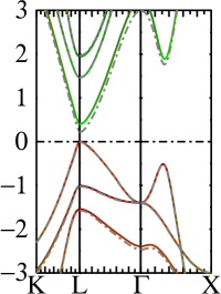
Figure 13: Energy band structure of PbTe in eV for (left) the LDA and (right) QSGW approximations. Colours correspond to projections onto L${}_{6}^{\pm}$ symmetry. L${}_{6}^{+}$ is comprised of Pb $s$ and the $t_{2g}$ part of the $d$ orbital, and Te $p$. L${}_{6}^{-}$ is comprised of Te $s$ and the $t_{2g}$ part of the $d$ orbital, and Pb $p$. The dashed lines show the effect of using a Dirac $p_{1/2}$ local orbital instead of the usual scalar relativistic one. Except for the addition of the Dirac $p_{1/2}$ orbital, the basis is similar to that used in Ref. [78]. It is a slight enlargement over the default basis, including $g$ orbitals on Pb and Te and a $6s$ local orbital on Te. These extra orbitals widen the gap relative to the default basis by $\sim$0.1 eV.

3.10 The PMT Method

In the introduction it was noted that the LAPW and Questaal’s generalised LMTO method are essentially the same except for the choice of envelope functions. LMTO’s are much more compact, and require a much smaller Hilbert space, but they suffer from problems with basis set completeness. An obvious alternative is to combine the two basis sets; this is the “PMT basis” [54]. This can be accomplished in practice quite neatly, because Questaal’s standard $\mathcal{H}_{L}$ require a one-centre expansion, Eq. (142), more general than simple LMTO’s (Eq. (1)). Plane waves can be expanded in polynomials $P_{kL}$ in a similar manner, as can other kinds of envelope functions. Thus the method provides a unified framework to seamlessly mix different kinds of envelope functions. Expressions for total energy, forces, assembling output density, etc, remain unchanged. The procedure is described in more detail in Ref. [54]; here we focus on the primary strengths and weaknesses of the method, using the total energy calculated for SrTiO₃ shown in Fig. 14 for discussion. It was redrawn from Ref. [54]. Four basis sets were chosen, ranging from pure LAPW (’null’) to a moderately large basis of 75 smooth Hankels $N(\mathcal{H}_{L})$ + 6 local orbitals.

basis	character of $\mathcal{H}_{L}$	$N(\mathcal{H}_{L})+N(\text{LO})$
null	no $\mathcal{H}_{L}$	6
hyper	sp on O only	18
small	spd on all atoms	51
large	+2${}^{\text{nd}}$ spd (spd on Ti)	81

Table 5: Nature and size of different basis configurations for the case of SrTiO₃.

Advantages of PMT

As expected, Questaal’s purely atom-centred basis is vastly more compact than a pure LAPW basis (Fig. 14). Even a tiny basis of just O sp states dramatically improves on the convergence of the LAPW basis. PMT offers a marked advantaged from LAPW perspective: by augmenting that basis by a few functions. From the atom-centred perspective Questaal’s standard moderately large basis misses about 5 mRy/atom in total energy, showing that it is not complete. Finally the figure shows that adding $\mathcal{H}_{L}$ continues to dramatically improve the convergence until the standard minimal basis of $\mathcal{H}_{L}$ is reached (single spd function on each atom). Beyond that initial rapid gain, it doesn’t seem to matter much whether the basis is increased by adding PW or more $\mathcal{H}_{L}$ (compare blue-solid and green-dashed lines).

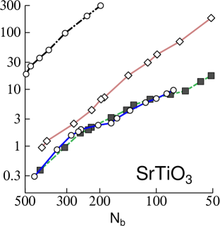
Figure 14: Deviation $\Delta{}E$ from fully converged total energy/atom, in mRy, vs total number of basis functions (PW + $\mathcal{H}_{L}$ + LO) $N^{\Gamma}_{\rm b}$ at $\Gamma$. Black-dashed, peach-solid, green-dashed, and blue-solid correspond respectively to the null, hyper, small, and large basis sets. $\Delta{}E$ is drawn on a log-log scale as a function plane-wave cutoff, denoted as $1/\text{N}_{\text{b}}$. $\text{N}_{\text{b}}$ is the total number of basis functions PW+$\mathcal{H}_{L}$+LO at the $\Gamma$ point.

Drawbacks of PMT

While they are far more efficient than ordinary LAPWs, PMTs show less promise than was initially hoped for.

• Compactness: LAPWs are not “intelligent”, i.e. tailored to the potential, and therefore convergence is slow in the basis size. Also their extended range precludes the advantages of short-ranged functions.

• Over-completeness: PMT has difficulties when $\mathcal{H}_{L}$ and PWs are both sizeable. This is because they span much the same Hilbert space. Workarounds (reducing the Hilbert space by projecting out parts that contribute to a small overlap) have been implemented, but they are inefficient and somewhat finicky—e.g. energy may not vary smoothly with the change in a nuclear coordinates.

• Interpolating $\Sigma_{0}$: in QSGW context, the ability to interpolate the QSGW self-energy $\Sigma_{0}$ is degraded. A workaround has been made for this problem also (Ref. [79]) by projecting $\Sigma_{0}$ onto the MTO part of the eigenfunctions, interpolating it, and re-embedding. Information is lost in the projection/re-embedding step, resulting in ambiguities. A much better way to address difficulties with interpolation is to construct very short-ranged, compact functions. This is shown clearly in Sec. 3.12.

In summary, PMT does best when treated as a slight augmentation of either the LAPW limit, or the MTO limit. Adding a few PWs with a low cutoff (2 Ry) was useful in our participation in the Delta Codes project (Sec. 3.13) particularly for the molecular solids such as N₂ which consist of 90% interstitial, or even more. Questaal’s pure MTO basis does not handle those compounds that accurately.

3.11 Floating Orbitals

While the PMT method can make the basis nearly complete, it causes severe difficulties when interpolating the QSGW $\Sigma_{0}$ to an arbitrary $k$. An alternative is to add “empty” sites — points outside augmentation spheres where extra $\mathcal{H}_{L}$ can be added to the basis. These sites have no augmentation spheres; they only enhance completeness in the interstitial. They are more ad hoc than plane waves (Sec. 3.10) particularly because there is no systematic path to convergence. Nevertheless they can be implemented efficiently; and Questaal has an automatic procedure to locate points to fill voids in the interstitial. In practice we use floating orbitals to converge QSGW self-energies with respect to the single-particle basis, in open systems. Their effect at the LDA level is usually not large, unless systems are very open or very accurate total energies are required. But for QSGW, where the potential depends on unoccupied states as well as occupied ones, it makes more of a difference, e.g correcting the fundamental gap in Si by of order 0.1 eV. We expect that the need for floating orbitals in such systems will be obviated by the new JPO basis. A precursor to it is discussed next.

3.12 Screened, Short-ranged Orbitals in the Full-Potential Framework

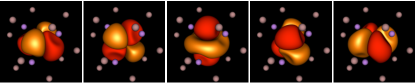
Figure 15: Screened $d$ envelope functions, $xy$, $yz$, $3z^{2}{-}1$, $xz$, and $x^{2}{-}y^{2}$, for a zincblende lattice. See also Fig. 5.

Building on the success of the “screening” of LMTOs in the ASA (Sec.2.9), we have developed an analogue within the full-potential LMTO framework. As in the ASA case, “screening” does not alter the Hilbert space but renders basis functions short ranged. Screening is a precursor to the next-generation JPO basis, which will alter the Hilbert space, rendering it significantly more accurate for the same rank of Hamiltonian. JPOs are still in development; the method will be presented in a future work. They have the following properties:

• they solve the SE with a (nearly) optimal number of basis functions for a given accuracy in the four dimensions $({{\mathbf{r}}},E)$;

• they are very short ranged (see Figs. 5 and 15); and

• they are atom centred with a definite $L$ character on their own MT sphere.

This provides a framework for exploiting the many advantages inherent in a short ranged basis sets. They can be used as projectors, replacing Wannier functions; they can be used to construct minimal Hamiltonians; near-sightedness can be exploited to make very efficient $O(N)$ solvers in DFT and $O(N^{3})$ solvers in GW and GW+BSE. That the basis functions are associated with a definite $L$ character is important, for example, when singling out a correlated subspace.

Screening of the $\mathcal{H}_{L}$ works in a manner similar to screening traditional $H_{L}$ because $\mathcal{H}_{L}$ asymptotically approaches a $H_{L}$ for large $r$ (Fig. 10). $\mathcal{H}_{L}-H_{L}$ decays approximately as a Gaussian of radius $r_{s}$: for traditional values of $r_{s}$ ($r_{s}\lesssim 2s/3$) it becomes negligible beyond first-neighbour distances. The screened $\mathcal{H}^{\alpha}_{L}$ employ the expansion coefficients $S^{\alpha}$ in the same manner as in the ASA (Sec. 2.9), so they have essentially the same range. What is sacrificed is the reinterpretation of screening in terms of hard core radius (Sec. 2.10.5), but this has no effect because the Hilbert space is unchanged. JPOs improve on the screened $\mathcal{H}^{\alpha}$ by restoring this condition and exploiting it to make the kinetic energy continuous everywhere.

Screening makes it possible to avoid Ewald summation otherwise necessary in the unscreened FP case (Appendix C). Also, one-centre expansions are made more efficient. By writing $\mathcal{H}^{\alpha}=\left\{\mathcal{H}^{\alpha}-{H}^{\alpha}\right\}+{H}^{\alpha}$, the first term which involves $\mathcal{H}$, must be expanded in the more cumbersome polynomials $P_{kL}$ (Eq. (145)). In the screened case the difference becomes short-ranged and can be dealt with efficiently in real space. The latter can use the simpler expansion Eq. (42).

A restriction in transformation is that all functions of a given $\kappa$ must share the same Hankel energy, while the traditional basis allows arbitrary choice for each orbital. However, this restriction is fairly mild because of the extra flexibility $\mathcal{H}_{L}$ have through the choice of $r_{s}$, which the ${H}_{L}$ do not. The $r_{s}$ strongly affect the kinetic energy near the MT boundary (Fig. 10), and the results are more sensitive to that choice than to the Hankel energy.

One large advantage of the transformation is that $\mathcal{H}^{\alpha}$ becomes short enough ranged so that matrix elements

$$\Sigma_{0;RL,R^{\prime}L^{\prime}}^{\alpha}=\left<\mathcal{H}_{RL}^{\alpha}|\Sigma_{0}|\mathcal{H}_{R^{\prime}L^{\prime}}^{\alpha}\right>$$

are limited by the range of the physical $\Sigma_{0}({{\mathbf{r}}},{{\mathbf{r}}}^{\prime})$, and not by the basis set. $\Sigma_{0;RL,R^{\prime}L^{\prime}}^{\alpha}$ turns out not to be very long ranged, as suggested some time ago by Zein et al. [80]. Fig. 16 shows how the bandgap in NiO evolves with range cutoff $R_{\text{cut}}$, defined as follows. $\Sigma_{0;RL,R^{\prime}L^{\prime}}^{\alpha}$ is initially computed without range truncation. Then matrix elements of $\Sigma_{0;RL,R^{\prime}L^{\prime}}^{\alpha}$ are set to zero for $|{{\mathbf{R}}}-{{\mathbf{R}}}^{\prime}|>R_{\text{cut}}$, and the band structure is calculated. As Fig. 16 shows, the bandgap $E_{G}$ converges slowly with $R_{\text{cut}}$ in the traditional $\Sigma_{0;RL,R^{\prime}L^{\prime}}^{\alpha{=}0}$ case, but for $\Sigma_{0;RL,R^{\prime}L^{\prime}}^{\alpha}$, $E_{G}$ is already reasonably converged including first and second neighbours. Note that for $R_{\text{cut}}{\to}\infty$, the two methods yield the same result, as the screening transformation does not change the Hilbert space.

One powerful feature of lmf is its ability to interpolate $\Sigma_{0}$. As noted in Sec. 4.2, some compromises must be made because the high-energy parts of $\Sigma^{nn^{\prime}}_{0}$ do not interpolate well, and elements above an energy threshold (of order 2 Ry) must be set to zero. The screening mitigates this difficulty; it appears that the energy threshold can be taken to $\infty$. The difference is not large, but in small bandgap cases where the precision of the method is very high, agreement with experiment may be limited by this difference.

The short range of $\Sigma_{0;RL,R^{\prime}L^{\prime}}^{\alpha}$ can be used to much advantage: we realise from the properties of Fourier transforms that the number of $k$ points directly translates into the number of neighbours in real space. Because $\Sigma_{0;RL,R^{\prime}L^{\prime}}^{\alpha}$ is short ranged, it converges faster in the $k$ mesh than $\Sigma_{0;RL,R^{\prime}L^{\prime}}^{\alpha{=}0}$, which saves significantly on computational effort. Also explicitly semilocal algorithms can be constructed, greatly reducing the cost to make $\Sigma_{0}$.

At present the short ranged screened smooth Hankel functions shine the most when used to represent the QSGW self-energy $\Sigma(\omega,q)$ and interpolate it at intermediate $q$ points not directly calculated in the heavy GW step. The interpolation process is significantly simplified and ambiguity is removed because the high energy $\Sigma$ no longer needs diagonal approximation, there is no need to define energy threshold and there is no loss of information due to discarding the off-diagonal parts. This does add to the computing effort for directly computed QSGW $\Sigma(\omega,q)$ because no states are excluded and matrix sizes increase respectively. To counter that, significantly fewer $\Sigma(q)$ need to be computed exactly, in our experience an equivalent result can be achieved by using only a half or in cases even a quarter of the original BZ sampling in each direction, for cells with few symmetry operations the savings add up quickly considering that the GW walks over pairs of $q$ points (quadrupling the total number of points for low symmetry cells). Performance can be further improved by still utilising the diagonal approximation to $\Sigma(\omega,q)$ because the interpolation is excellent and the high energy part only weakly affects states near $E_{F}$. To show the quality of the QSGW $\Sigma(\omega,q)$ expansion in the new, screened basis and the conventional unscreened, we plot the dependence of the NiO bandgap as a function of the truncated self energy in Fig. 16.

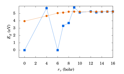
Figure 16: NiO bandgap in eV as a function of the range truncated self-energy represented in the conventional and screened basis sets. The first point contains onsite terms only, the second adds first neighbours etc. The conventional basis shows erratic behaviour until at least the fourth neighbours are present.

At the LDA level, the better spatial localisation of screened basis function paves the way to efficient, real-space assembly of matrices (1 and 2 particle) while maintaining, and in cases improving, accuracy. The screened functions are also significantly less linearly dependent. The implementation is heavily vectorised and at present can handle a couple hundred atoms on a single node, with the scalability properly utilised the numbers can be an order of magnitude larger. For very large systems, it will be possible to construct $O(N)$ methods, but empirically it appears so far that systems of a few hundred atoms are probably still too small for such methods to be advantageous.

To summarise, our current screening transformation offers advantages of short-ranged basis sets. It is not yet optimally compact. However, the JPO basis, to be reported on soon, we believe will be nearly the most compact (optimal convergence for a given rank of Hamiltonian, and short range). We believe these advantages will be very significant, and obviate the need for enhancements such as plane waves (Sec. 3.10) or floating orbitals (Sec. 3.11) to obtain high accuracy.

3.13 Delta Codes Validation Exercise

The Delta Codes project [6] is a continuing effort to mutually validate the different electronic structure codes used in condensed matter and materials modelling. The first comparison has focused on the equations of state calculated for a selection of elemental solids. The relative agreement of different codes, including lmf, can be examined on the project site https://molmod.ugent.be/deltacodesdft. Agreement is quantified using an average “Delta value”—the integrated difference between equation of state curves over a specified volume range.

The calculated equations of states (scalar relativistic and PBE-GGA exchange-correlation are specified) agree extremely closely, particularly among the all-electron codes. The pseudopotential projects have also demonstrated precision very similar to the all-electron methods.

The Delta Codes test set has been carried out for lmf with an automatic setup, avoiding any system-specific modifications. The main settings defining the calculations are:

Sphere radii:

$s_{R}$ corresponding to touching spheres are used, evaluated at the smallest volume tested.

$\ell_{\text{max}}$:

The maximum $\ell$ for the basis functions is 1 for H and He, 2 for $Z<18$ and 3 otherwise. In each case, one higher $\ell$ is included in the partial wave expansion.

Semi-core states:

Local orbitals are effective for including semicore states in the valence. We recommend treating states as semicore whenever the leaked charge exceeds $0.002e$, or the eigenvalue is higher than $\sim-2$ Ry. For transition metals and f-electron systems, the inclusion of high-lying $\ell=2$ or $3$ conventional local orbitals can significantly improve accuracy and these are added by default for these groups of elements.

Molecular cases:

For cases where the touching muffin-tin spheres fill less than 30% of the cell volume, an additional LAPW basis has been included. The LMTO basis was not designed for molecular systems — but the shortcomings of the LMTO basis can be easily rectified by the addition of small number of plane-waves.

Basis setup:

Basis parameters determined automatically as described below.

3.13.1 Choice of Basis Parameters

Questaal’s full-potential code allows two LMTO basis functions to be used per $\ell$. Each of these is defined by two parameters which must be chosen: the Hankel energy and the smoothing radius. Because the size of the LMTO basis is small, the choice of basis parameters can have a significant impact on accuracy. Different schemes for choosing basis parameters have evolved, of which the simplest is to fit the basis functions to the free atom wave functions. This provides one set of basis parameters for each $\ell$. The second set is obtained from the first by shifting the Hankel energy (typically by $-0.5$ to $-0.8$ Ry). This is a heuristic approach but it is automatic and effective and is the default.

An alternative method chooses smoothing radii directly from the potential. The gradient of the smoothed Hankel functions at typical muffin-tin sizes is sensitive to $r_{s}$ and variational freedom is obtained by differentiating the two sets of basis functions by $r_{s}$ instead of the Hankel energy. The smoothing radius describes the point where the basis function begins to deviate from the exponential, Hankel-like tail: this is similar to the behaviour of atomic eigenfunctions at their classical turning points.

Associating the smoothing radius with the classical turning point allows basis functions to be constructed that resemble atomic-like states at energies different to the atomic eigenvalues and the question of choosing suitable $r_{s}$ is translated into a determining a pair of reference energies—one each for the two basis sets per $L$. Energies of the valence states are typically in the range $0$ to $-2$ Ry, and choices for the reference energies of $E_{1}=-0.5$ and $E_{2}=-2.0$ result in accurate basis sets for most materials. In this scheme, the Hankel energy remains a free parameter but similar results are found for Hankel energies in the range $-0.1$ to $-1$ Ry.

The choice of reference energies can be automated by expressing them in terms of the atomic potential at the muffin-tin radius. One basis set is chosen with a higher reference energy, giving a more diffuse basis function, the other is setup at a smaller, more negative, energy which yields a smaller $r_{s}$ and a more tightly bound basis function. Because $v(s_{R})$ varies significantly across elements and materials, a proportional scheme is more suitable: e.g., $v(r_{s}^{1})=2v(s_{R})$ and $v(r_{s}^{2})=\frac{1}{2}v(s_{R})$; this algorithm is used for automating the DeltaCodes tests.

3.13.2 Comparison with LAPW Results

Figure 17 shows the “Delta values” for Questaal with respect to the LAPW code WIEN2K. The level of agreement is typical (or better) than most all electron methods involved in the validation exercise. In particular, the transition elements are extremely well represented by the smooth Hankel basis. Some of the first period and group VII cases involve molecular problems for which the muffin-tins fill a small fraction of the unit cell: the performance of the LMTO basis in these cases becomes sensitive to $r_{s}$ and $E$ choices. We do not attempt to choose optimal parameters, instead we include an additional LAPW (see Sec. 3.10), with cut-off 2 Ry or 4 Ry depending on the packing fraction. Au and group VI are outliers: in both cases the automatic basis setup generates basis functions that are rather too smooth to describe the tightly bound states in these elements. If necessary, improved performance can be obtained, thereby converging $V_{0}$ with respect to the basis, by adding plane waves.

In addition to confirming that the smooth Hankel basis is capable of high precision, the testing procedure also demonstrates that the automatic procedure for setting up the basis and setting various numerical parameters is highly reliable.

Figure 17: “Delta Codes” tests: integrated energy difference between the energy-volume curves calculated by lmf and WIEN2K [81], expressed in meV/atom; the average value is 0.62meV/atom.

4 GW and QSGW

The GW approximation (G=Green’s function, W=screened Coulomb interaction) is the first-order term in the formally exact diagrammatic expansion around some one-particle Hamiltonian $H_{0}$ [82].

Questaal’s GW formalism is explained in some detail in Ref. [83], and its implementation of quasi-particle self-consistent GW (QSGW) is explained in Ref. [84]. Here we recapitulate only the main points. From an implementation point of view, GW requires two-point functions, such as the susceptibility from which $W$ is made (Sec. 6). This entails an auxiliary product basis of wave function products. Most commonly plane waves are used to implement GW. In such a case the same basis for two-particle objects can be used, because a product of plane waves is another plane wave, but for all-electron methods this is not possible. Representation of these objects requires a basis spanning the Hilbert space of wave function products. Four-centre integrals (e.g. Eq. (LABEL:generalchi01q)) can be evaluated as integrals of pairs of product basis functions. This was first accomplished by Aryasetiawan [85] in an ASA framework, and extended by us [15] into a full-potential scheme.

In the ab initio context, GW has traditionally referred to a perturbation around the LDA: i.e. $H_{0}={H^{\text{LDA}}}$ so that $GW={G^{\text{LDA}}}{W^{\text{LDA}}}$, though in recent years hybrid functionals or LDA+U have become popular. It has become increasingly recognised that results depend rather strongly on the choice of $H_{0}$, or equivalently the $V_{\text{xc}}$ entering into it, by which we mean the beyond-Hartree parts of the effective potential. Thus the self-energy of $H_{0}$ is $\Sigma=V_{\text{xc}}$ in the language of many-body perturbation theory. The implications of starting point dependence are profound: the quality of GW depends on the quality of the reference. Moreover it is increasingly accepted that ${H^{\text{LDA}}}$ is only a good choice for $H_{0}$ for a very restricted materials class.

$GW$ is a perturbation theory, and usually only the lowest order perturbation (diagonal part of $\Sigma$ in the basis of the reference Hamiltonian) is kept. As a result eigenfunctions are not perturbed and the change in QP level ${\varepsilon_{kn}}$ is

$$\delta{\varepsilon_{kn}}=Z_{kn}[\langle\Psi_{kn}|\Sigma({{\mathbf{r}}},{{\mathbf{r}}}^{\prime},{\varepsilon_{kn}})-V_{\rm xc}^{\rm{LDA}}({{\mathbf{r}}})|\Psi_{kn}\rangle]$$ (173)

$Z_{kn}$ is the quasi-particle (QP) renormalisation factor

$$Z_{kn}=\left[1-\langle\Psi_{kn}|\frac{\partial}{\partial\varepsilon}\Sigma({{\mathbf{r}}},{{\mathbf{r}}}^{\prime},{\varepsilon_{kn}})|\Psi_{kn}\rangle\right]^{-1}$$ (174)

and accounts for the fact that $\Sigma$ is evaluated at ${\varepsilon_{kn}}$ rather than at the QP energy ${\varepsilon_{kn}}{+}\delta{\varepsilon_{kn}}$. Eq. (173) is the customary way QP energies are evaluated in $GW$ calculations. In Sec. VI of Ref. [56], we show that omitting the $Z$ factor is an approximate way to incorporate self-consistency, and thus should be a better choice than including it. As a practical matter it is also the case that results improve using $Z$=1.

Ref. [56] notes a serious drawback in the diagonal-only approximation: when levels in the reference Hamiltonian are wrongly ordered as they are, e.g. at the $\Gamma$ point in Ge, InN, and CuInSe₂, and the L point in PbTe [78] the wrong starting topology results in an unphysical band crossing in the GW QP levels. (See, for example an illustration for Ge in Fig. 6 of Ref. [56]). Something similar will happen for PbTe (Fig. 13). Moreover, the off-diagonal parts of $\Sigma$ can significantly modify the eigenfunctions and resulting charge density. This reflects itself in many contexts, e.g. strong renormalisation of the bandgaps in polar insulators such as TiSe₂ and CeO₂  [56]. It modifies orbital character of states near the Fermi energy in La₂CuO₄, and significantly affects how the metal-insulator transition comes about, when GW is combined with DMFT [86].

4.1 Need for Self-consistency

The arbitrariness in the starting point means that there is no unique definition of the GW approximation. Errors in the theory (estimated by deviations from experiment) can be fairly scattered for a particular choice of reference, e.g. LDA, making it unclear what the shortcomings of $GW$ actually are. Arbitrariness in the starting point can be surmounted by iterating $G$ to self-consistency, that is, by finding a $G$ generated by GW that is the same as the $G$ that generates it ($G^{\text{out}}$=$G^{\text{in}}$). But it has long been known that full self-consistency can be quite poor in solids [87, 88]. A recent re-examination of some semiconductors [89] confirms that the dielectric function (and concomitant QP levels) indeed worsen when $G$ is self-consistent, for reasons explained in Appendix A in Ref. [84]. Fully sc$GW$ becomes more problematic in transition metals [90]. Finally, even while scGW is a conserving approximation in the Green’s function $G$, in $W$ it is not: it violates the sum rule [91] and loses its usual physical meaning as a response function. As a result it washes out spectral functions in transition metals [90], often yielding worse results than the LDA.

A simple kind of self-consistency is to update eigenvalues but retain LDA eigenfunctions, as was first done by Aryasetiawan and Gunnarsson [92]. This greatly improves GW, especially in systems such as NiO where the LDA starting point is very poor. But it is only adequate in limited circumstances. In TiSe₂ it strongly overestimates the bandgap (see below), as it does in NiO [92]. An extreme case is CeO₂ where the position of the Ce $4f$ levels is severely overestimated; see Fig. 3 in Ref. [83]. The off-diagonal elements in $\Sigma$, which are needed to modify the eigenfunctions, can be very important.

Questaal employs quasiparticle self-consistency [16, 83, 84]: by construction, the reference $H_{0}$ is determined within GW as in the fully self-consistent case. But the proper $\Sigma{=}iGW$ cannot be used because it is energy dependent and non-Hermitian, thus falling outside of an independent particle picture. This causes GW to degrade, and higher-order diagrams are needed [87] to restore the quality of GW. But by quasiparticlising $\Sigma$ we can stay within a framework of perturbation around $H_{0}$ but choose $H_{0}$ in an optimal manner. QSGW quasiparticlises $\Sigma(\varepsilon)$ by approximating it by a static Hermitian potential as

$$\Sigma_{0}=\frac{1}{2}\sum_{ij}|\psi_{i}\rangle\left\{{{\rm Re}[\Sigma({\varepsilon_{i}})]_{ij}+{\rm Re}[\Sigma({\varepsilon_{j}})]_{ij}}\right\}\langle\psi_{j}|$$ (175)

which is the QSGW form for a static $V_{\text{xc}}$. This process is carried out to self-consistency, until $\Sigma_{0}^{\text{\,out}}=\Sigma_{0}^{\text{\,in}}$. Given $\Sigma_{0}$, a new effective Hamiltonian can be made, which generates a new $\Sigma_{0}$:

$${\Sigma_{0}}\to{G_{0}}\to\Sigma=i{G_{0}}W[{G_{0}}]\to{\Sigma_{0}}\dots$$ (176)

$\Sigma_{0}$ is nonlocal with off-diagonal components; both of these features are important.

TiSe₂ is an interesting case where self-consistency becomes critical. It is a layered diselenide with space group $P\bar{3}m1$. Below $T_{c}$=200K, it undergoes a phase transition to a charge density wave, forming a commensurate $2{\times}2{\times}2$ superlattice ($P\bar{3}c1$) of the original structure. It has attracted a great deal of interest in part because the CDW may to be connected to superconductivity.

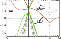
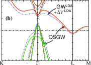
Figure 18: TiSe₂ energy bands in eV for the undistorted $P\bar{3}c1$ structure. $(a)$: solid lines are LDA results, with red and green depicting a projection onto Ti and Se orbital character, respectively. Blue dashed line shows shifts calculated in the $GW$ approximation based on the LDA. $(b)$: blue dashed line shows results from $GW$ based on the LDA (same self-energy as in panel $(a)$), with an extra potential $\Delta V^{\text{LDA}}$ deriving from a charge density shift computed from the rotation of the LDA eigenvectors. Solid lines are QSGW results, with the same colour scheme as in panel $(a)$.

How the CDW affects the energy band structure is a source of great controversy. It is accepted experimentally that in the $P\bar{3}c1$ phase, TiSe₂ is semiconductor with a gap of $\sim$0.15 eV. Above $T_{c}$ whether intrinsic TiSe₂ has a gap is not settled. On the theoretical side, the CDW makes TiSe₂ an unusual materials system: DFT predicts a metal in both $P\bar{3}m1$ and $P\bar{3}c1$, as expected, but a recent ${G^{\text{LDA}}}{W^{\text{LDA}}}$ calculation [93] predicts $P\bar{3}m1$ to have a small positive gap. We have revisited this problem and confirmed the findings of Ref. [93] at the ${G^{\text{LDA}}}{W^{\text{LDA}}}$ level. However, at the QSGW level, TiSe₂ is a metal in the ideal $P\bar{3}m1$ phase. This is atypical for insulators: usually self-consistency widens the gap, as has long been known (see Fig. 1 in Ref. [83]). The origin can be traced to the modification of the LDA eigenfunctions by off-diagonal elements $\Sigma_{n\neq n^{\prime}}$, which modify the density $n(r)$. To see approximately the effect of the density change, assume LDA adequately describes ${\delta}V^{\text{eff}}/{\delta}n$ (this is the inverse susceptibility, the charge analogue of Eq. (181)). For a fixed $\Sigma^{0}$, we can estimate the effect of the change ${\delta}n$ renormalising the $V^{\text{eff}}$ through the change

$$\delta{\Sigma}\approx\left\{{\Sigma_{0}}-V_{\text{xc}}^{\text{LDA}}[{n^{\text{LDA}}}]{\text{ }}\right\}+V_{\text{xc}}^{\text{LDA}}[n^{GW}]$$

This is accomplished in a natural way with the Questaal package. The quantity in curly brackets is generated by GW in the first QSGW cycle, and lmf treats this term as an external perturbation. Running lmf to self-consistency allows the system to respond to the potential and screen it, yielding $n^{GW}$.

The result of this process is shown as a dashed line in Fig. 18(b). It bears a close resemblance to the full QSGW result, including the negative gap. We will show elsewhere that TiSe₂ is an insulator in the $P\bar{3}c1$ phase only as a consequence of lattice displacements relative to the symmetric $P\bar{3}m1$ phase.

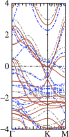
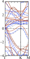
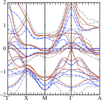
Figure 19: Energy band structure, in eV, of majority-spin MnAs (left), minority-spin MnAs (middle) and nonmagnetic FeTe (right) in (a) the QSGW approximation (orange solid lines), ${G^{\text{LDA}}}{W^{\text{LDA}}}$ (dashed blue lines), and the LDA (light dashed grey lines). ${G^{\text{LDA}}}{W^{\text{LDA}}}$ was calculated from the LDA, but including the off-diagonal components of $\Sigma$ with $Z$=1. It is the 0^th iteration of the QSGW self-consistency cycle.

GW is used less often in metals. As in the insulating case, GW based on DFT can sometimes work well, as it apparently does for SrVO₃ [94]. But the range of applicability is limited, and indeed ${G^{\text{LDA}}}{W^{\text{LDA}}}$ can yield catastrophically bad results. Two cases in point are MnAs and FeTe. Fig. 19 shows LDA, ${G^{\text{LDA}}}{W^{\text{LDA}}}$, and QSGW energy bands near $E_{F}$; they are mostly of Mn or Fe $3d$ character. In the ${G^{\text{LDA}}}{W^{\text{LDA}}}$ case, $E_{F}$ must be adjusted to conserve charge. (The shift is large, of order 1 eV.) Consider MnAs first. The majority and minority $3d$ bands lie at about $-$1.5 eV and +1 eV in the LDA. This exchange splitting is underestimated: QSGW increases the splitting, putting bands at about ($-$2.5,1.5) eV while ${G^{\text{LDA}}}{W^{\text{LDA}}}$ does the opposite, reducing the splitting relative to LDA. Also, the Fermi surface topology is poor: the hole pocket at $\Gamma$ disappears, and the one at K is similar to the LDA. FeTe fares no better. ${G^{\text{LDA}}}{W^{\text{LDA}}}$ is somewhere intermediate between LDA and QSGW. Most important is the unphysical, dispersionless band at $E_{F}$ on the X-M line, which yields a nonsensical Fermi surface. In both of these materials, the LDA describes the electronic structure better than ${G^{\text{LDA}}}{W^{\text{LDA}}}$.

Figure 20: Ionisation potential, IP, of TM atom and heat of formation ${\Delta}E$ of transition-metal dimers computed within the RPA, using the molgw code selecting various choices of starting point. Note the dramatic difference between Hartree-Fock and the PBE starting points. Of the common semi-empirical functionals, HSE06 (not shown) is the closest to QSGW. Data were compared to reference CCSD(T) for the ionisation potential and experiment for ${\Delta}E$.

Ambiguities in the starting point make it difficult to know what errors are intrinsic to the theory and which are accidental. The literature is rife with manifestations of this problem; see e.g. Ref. [95]. Self-consistency (mostly) removes the starting-point dependence so that the errors intrinsic to the $GW$ approximation can be best elucidated. Moreover, QSGW should yield better RPA total energies on average than those calculated from other starting points, because the path of adiabatic connection is optimally described through QSGW [84]. To better illustrate these points Fig. 20 shows the ionisation potential of 3$d$ transition metal atoms and the heat of formation of 3$d$-O dimers, computed by the molgw code [96]. We focus on these properties because it is known, e.g. from Ref. [97], that the RPA tends to systematically overbind, and the error is connected with short-ranged correlations. The ionisation potential and the dimer formation energy, both of which benefit from partial cancellation of such errors, are much better described.

Note the dramatic difference between choice of a Hartree-Fock or the PBE functional. As for the superiority of QSGW, Fig. 20 generally bears this argument out, though there are some surprises, e.g. the heat of formation from RPA@PBE deviates less from CCSD(T) results than QSGW. QSGW does not describe Cr well, probably because spin fluctuations are important there (Sec. 4.4), which skews the statistics with this small sample. The discrepancies are small enough that incomplete convergence in the basis set (results in Fig. 20 were obtained with a triple-$\zeta$ basis) are of the same order and could account for some of the results. The ionisation potential of simple $sp$ atoms was analysed in Ref. [98], where it was computed from RPA total energy differences, compared to the eigenvalue of the GW one-particle Hamiltonian. There also it was shown QSGW significantly improves on RPA@HF, and also that QSGW is slightly biased towards Hartree-Fock, reflecting a slight tendency to underestimate screening. This is consistent with the tendency for QSGW to overestimate bandgaps. Koval et al.[99] found somewhat different results for small, second-row molecules.

QSGW-RPA is not accurate enough to reach quantum chemical accuracy, $\sim$1 kcal/mol. The addition of ladders should considerably improve on the RPA’s known inadequacy in describing short-ranged correlations. It has long been known that ladders dramatically improve the dielectric function $\epsilon(\omega)$ ($\epsilon(\omega)$ and G enter in the coupling constant integration for total energy) and it would be interesting to explore if such low-order diagrams in a QSGW framework are sufficient to capture total energy to this accuracy.

While self-consistency does largely surmount starting-point dependence (it was recently shown to be the case for some insulators using Hartree-Fock and LDA as starting points [100]), but it is not strictly true that it does. The QSGW $H_{0}$ or $G_{0}$ has a Hartree Fock structure, and it can get stuck in metastable valleys in the same way as Hartree Fock; an example are the dual low-spin and high-spin states found for FeSe (Sec. 4.4). Also, in strongly correlated systems $\Sigma(\varepsilon)$ can vary rapidly with energy. There can be more than one $\epsilon_{i}$ that forms a stationary point. This happens, for example, in CuO. It is usually an indication that the ground state is not well described by a single Slater determinant. QSGW restricts $G_{0}$ to a single determinant, and there is no longer an unambiguously optimal choice when there are two or more equally strongly competing ones.

There is no unique prescription for quasiparticlisation, but Eq. (175) minimises the difference between the full $G$ and $G_{0}$ according a particular choice of norm. Recently it was shown [101] that Eq. (175) minimises the absolute value of the gradient of the Klein functional over all possible spaces of non-interacting Green’s functions. There are formal reasons ($Z$ factor cancellation [84] and conserving sum rule [91]) why quasiparticlisation should be better; there is also abundant empirical evidence, that quasiparticle self-consistency performs better than full self-consistency [90, 102, 89], and the particular construction Eq. (175) is an optimum one.

QSGW has been implemented in numerous electronic structure packages, e.g. the spex code [103], the Abinit code [104], VASP [105], recently in the Exciting code [100], and also in molecules codes such as molgw [96] and NWChem [99]. For solids perhaps the most rigorous implementation is the spex code, which can use a local Sternheimer method to rapidly converge the calculation of the dielectric function [106]. As attempts to make efficient schemes that are also well converged, e.g. to calculate the RPA total energy, the local Sternheimer method will likely emerge as being very significant over time.

4.2 Questaal’s QSGW Implementation

Questaal’s implementation of QSGW evolved from the ecalj package, developed by Kotani and coworkers in the early 2000’s out of Aryasetiawan’s GW-ASA code [13], which in turn was developed from the “Stuttgart” LMTO code. The original ecalj package can now be found at https://github.com/tkotani/ecalj/. As of this writing we maintain the GW code as a separate branch (Fig. 21). In its present form the GW part of Questaal’s QSGW implementation operates independently, receiving information about eigenfunctions and eigenvalues, and returning response functions or a self-energy. As for the QSGW cycle, one cycle occurs in three parts.

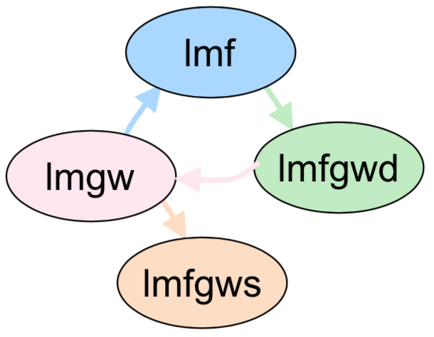
Figure 21: Questaal’s QSGW cycle. lmf generates a new self-consistent density and noninteracting $H_{0}$ for a fixed $\Sigma_{0}$; lmfgwd generates information about the eigenfunctions $\Psi$ corresponding to $H_{0}$, and lmgw receives the output of lmfgwd and uses it to make a new $\Sigma_{0}$. lmgw can also generate response functions and the fully dynamical self-energy $\Sigma^{nn}(\omega)$. lmfgws is a post-processing code that yields observables computed from the interacting $G$, where $G^{-1}={G_{0}}^{-1}+\Sigma^{nn}(\omega)-{\Sigma_{0}}^{nn}$.

Rather than storing $\Sigma_{0}$ on disk, $\Sigma_{0}-V_{\text{xc}}$ is stored ($V_{\text{xc}}$ usually being the LDA potential). Thus lmf generates its customary LDA Hamiltonian, and adds $\Sigma_{0}-V_{\text{xc}}$ to it. In practice this is accomplished by reading $\Sigma_{0}-V_{\text{xc}}$ on the mesh of $k$ points where it was generated, and inverse Bloch-summing to make $\Sigma_{0}-V_{\text{xc}}$ in real space. Then $\Sigma_{0}-V_{\text{xc}}$ can be interpolated to any $k$ by a forward Bloch sum. This is a unique and powerful feature, as it makes it possible to generate QSGW eigenfunctions and eigenvalues at any $k$. There are some subtleties in this step: the interpolation does not work well if all the $\langle n|\Sigma_{0}^{nn^{\prime}}|n^{\prime}\rangle$ are included. It is solved by rotating to the LDA eigenfunctions, and zeroing out $\Sigma_{0}^{n{\neq}n^{\prime}}$ for $n$ or $n^{\prime}$ whose energy exceeds a threshold, $E_{\text{cut}}$; i.e. diagonal-only approximation for high-energy subblocks of $\Sigma_{0}$. $E_{\text{cut}}$ is typically ${\sim}2$ Ry; convergence can be checked by varying $E_{\text{cut}}$. The prescription is explained in detail in Sec. IIG of Ref. [84]. The error is connected to the relatively long range of the smooth Hankel envelopes. Preliminary tests using short-ranged, screened Hankels indicate that this truncation is no longer needed.

Typically $\Sigma_{0}$ is a smoother function of $k$ than the kinetic energy. Thus the $k$ mesh on which $\Sigma_{0}$ is made can usually be coarser than the $k$ mesh. Because of its ability to interpolate, lmf and lmgw operate with independent meshes.

4.3 Successes of QSGW

QSGW has the ability to calculate properties for a wide variety of materials classes in a manner that no other single theory can equal. It consistently shows dramatic improvement relative to DFT and extensions such as hybrid functionals or LDA-based GW. Atomic ionisation potentials [98], quasiparticle (QP) levels, Dresselhaus coefficients in semiconductors [107, 108, 109]; band offsets at the Si/SiO₂ interface [104], magnetic moments and spin wave excitations [110, 111]; tunnelling magnetoresistance [112]; impact ionisation [113]; electric field gradients and deformation potentials [114], spectral functions [115], and dielectric response [116]. Its superior ability to yield QP levels and DOS made it possible to accurately determine valence maximum in SrTiO₃ [117]. In contrast to ${G^{\text{LDA}}}{W^{\text{LDA}}}$, QSGW is uniformly reliable with systematic errors (see Sec. 4.4). Fundamental gaps are usually in very good agreement with experiments, though they are systematically overestimated (see Fig. 1 in Ref. [83]), even in the strongly correlated M1 phase of VO₂ [118, 119, 120], where spin fluctuations are not important. It properly narrows the bandwidth of localised $d$ bands and widens it in wide-gap semiconductors [117] and graphene [121].

QSGW can predict properties inaccessible to ${G^{\text{LDA}}}{W^{\text{LDA}}}$, such as magnetic ground state [115] and charge density. Fig. 22 shows the density calculated by QSGW in the plane normal to [001] for antiferromagnetic NiO and CoO. Two prominent features are seen: (1) NiO is much more spherical than CoO, and the density contours for CoO are elongated along the [110] line. Both of these findings are consistent with $\gamma$ ray measurements [122, 123].

Figure 22: Self-consistent charge density in antiferromagnetic NiO (left) and CoO (right), in the plane normal to [001], computed by QSGW. The Ni (Co) nucleus lies at the centre of the Figure.

It was noticed early on [83] that QSGW has a systematic tendency to overestimate bandgaps in semiconductors and insulators. To what extent dispersions are well described is much less discussed, in part because there is a limited amount of experimental data reliable to the precision needed. Perhaps the best materials family to serve as a benchmark are the zincblende semiconductors, where critical-point analysis of the dielectric function has been used to accurately measure in most zincblende semiconductors, not only the $\Gamma$-$\Gamma$ ($E_{0}$) transition but also the L-L ($E_{1}$) and X-X ($E_{2}$) transitions, as indicated in Fig. 23, which presents the QSGW and LDA bands compared with ellipsometry and photoemission data.

Figure 23: QSGW energy band structure of GaAs compared with ellipsometry data and photoemission data (open and closed circles). Dashed Grey lines are LDA bands.

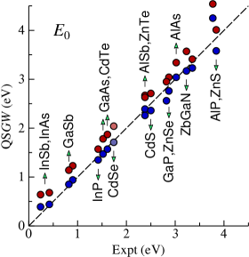
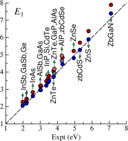
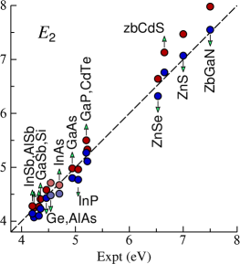
Figure 24: Transitions $E_{0}$, $E_{1}$ and $E_{2}$ transitions in a zincblende semiconductor compared with critical point measurements. Red and blue circles are QSGW results, and QSGW with $\Sigma_{0}^{\text{scaled}}$ (Eq. (177)), respectively.

Fig. 24 shows that tendency to overestimate $E_{0}$ and $E_{1}$ is systematic and uniform, but there is less uniformity in $E_{2}$. Usually $E_{0}$ can be precisely measured; similarly for $E_{1}$ because there is a sizeable volume of $k$ near L where valence and conduction bands disperse in a parallel manner. $E_{2}$ is more difficult, and values are less certain. That being said, the data suggest $E_{0}{-}E_{2}$ is, on average, about 0.1 eV below experiment. We have found that this error is, at least in part, due to the necessity of truncating high-lying parts of the off-diagonal $\Sigma_{0}$; see $E_{\text{cut}}$, Sec. 4.1. It has recently become possible to re-evaluate this because a short-range basis was recently developed (Sec. 3.12) appears to interpolate $\Sigma_{0}$ allowing $E_{\text{cut}}{\to}\infty$.

Also reliably measured are the electron effective mass $m_{e}^{*}$ (hole masses are much less well known), and for some systems, the nonparabolicity parameter $\alpha$, characterising deviations from parabolicity near $\Gamma$, and defined as $k^{2}/m^{*}=\varepsilon(k)[1-\alpha\varepsilon(k)]$ where $\varepsilon$ is the band energy relative to the conduction band minimum. $\alpha$ is an important quantity in several contexts, particularly hot-electron semiconductor electronics. Unfortunately $\alpha$ is difficult to measure, and values reported are usually some scalar average of the second rank tensor. Where it has been measured QSGW (or scaled QSGW, Eq. (177)) seems to predict $\alpha$ to within the experimental resolution; see e.g. Table 6 for GaAs. Fig. 25 compares QSGW and experimental effective masses for various semiconductors. Conduction band masses are well described, although there is a systematic tendency to underestimate it, connected to the tendency to overestimate $E_{G}$.

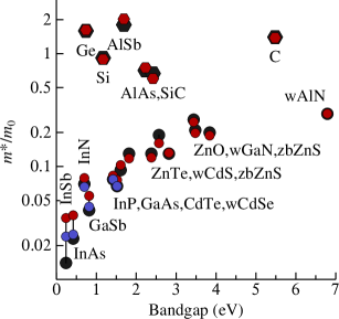
Figure 25: Conduction band effective masses of selected zincblende compounds compared against experiment. Red and blue circles are QSGW results, and QSGW with $\Sigma_{0}^{\text{scaled}}$; black circles are experimental values.

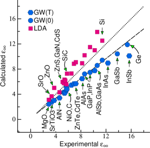
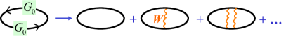
Figure 26: Dielectric constant $\epsilon_{\infty}$ compared to experiment. Blue are QSGW results; red are LDA results. Also shown are the ladder diagrams that modify bubbles in the polarisability, left out in the RPA.

Most of this error can be traced to the RPA approximation to the dielectric function. The optical dielectric constant $\epsilon_{\infty}$ (Eq. (192)) in the $\omega{\to}0$ limit is uniformly too small by a factor ${\sim}0.8$ for many kinds of semiconductors and insulators (Fig. 26). Plasmon peaks in $\text{Im}\epsilon(\omega)$ are almost universally blue shifted [124, 125] because the RPA omits the attraction between electron-hole pairs in their virtual excitations. A simple Kramers-Kronig analysis shows that as a consequence, $\epsilon_{\infty}{=}\mathrm{Re\,}\epsilon(\omega{\to}0)$ should be underestimated. Indeed we find that to be the case, but remarkably $\epsilon_{\infty}$ is consistently underestimated, by a nearly universal factor of 0.8. This is what motivated a hybrid of LDA and QSGW functionals [107]

$$\Sigma_{0}^{\text{scaled}}=0.8\,\Sigma_{0}+0.2\,V^{\text{LDA}}_{\text{xc}}$$ (177)

The reasoning is since $W$ is dominated by the $q{\to}0,\omega{\to}0$ limit, scaling $W$ by 0.8 justifies Eq. (177). In practice, it seems that the tendency to overestimated bandgaps is almost completely ameliorated in these systems (compare red and blue circles, Fig. 24, as is the tendency to underestimate $m_{c}^{*}$. Exceptions are the small-gap InAs in InSb, where relative errors in bandgaps are still not small even with the 0.8 scaling.

The hybrid scheme does a stellar job in many contexts: it improves on bandgaps in semiconductors (Fig. 24) and predicting the Dresselhaus splitting in sp semiconductors [107]. But the scheme is empirical, and it is limited. It does not properly correct the blue shifts in $\epsilon(\omega)$ or take into account other excitonic effects and fails to bring bandgaps in close agreement with experiment in systems with strong spin fluctuations such as CoO or La₂CuO₄, and deep states such as the Ga $3d$ shift farther from experiment (see Table below). Recent work [102, 126] shows that the great majority of the error in charge susceptibility can be accounted for by ladder diagrams. (In the case of polar semiconductors there can also be a significant renormalisation of the gap from the Frölich interaction [127, 128]; the electron-phonon interaction has a modest effect in other semiconductors, especially compounds with second row elements [129], diamond being the largest.) Without ladders the low-frequency dielectric constant is — almost universally — about 80% of experiment ( [130]). As we will show elsewhere [126] the addition of ladders in W seem to dramatically improve on the charge channel even in strongly correlated cases such as CoO. VO₂ is an excellent test bed for optics: it has strong correlations in the monoclinic phase; yet, the conductivity is well described by nonmagnetic QSGW, provided ladders are taken into account [119].

Below we present more detailed properties of the band structure obtained from classical QSGW on a single system, selecting GaAs because reliable measurements are available and it is representative of results obtained for the entire family of zincblende semiconductors (Table 6). We observe the following:

1. dispersions $\Gamma$-L and $\Gamma$-X are mostly well described, and vastly better than the LDA (which predicts the $\Gamma$-X dispersion to be 1 eV);

2. the valence bands match photoemission data to within experimental resolution;

3. the Ga $3d$ (see Table below) is pushed down relative to the LDA and also relative to ${G^{\text{LDA}}}{W^{\text{LDA}}}$. Binding of shallow core-like states on e.g. Cd, Zn, and Cu is underestimates by ${\sim}0.4$ eV; for deeper states such as Ga $3d$ it is larger. It was shown in Ref. [131] that a low-order vertex correction to GW accounts for most of this discrepancy, at least for shallow core-like levels;

4. conduction bands are slightly overestimated and the mass slightly too large; and

5. the nonparabolicity parameter $\alpha$ was calculated along the [001], [110], and [111] directions. It varies $\sim$30% for different directions, but since only scalar quantities are reported, we take a geometrical average. $\alpha$ is very sensitive to $m^{*}$, so we can expect it to be underestimated a little; this turns out to be the case. Using Eq. (177) all three quantities align well with experiment.

	$E_{G}$	$m^{*}/m$	$\alpha$	Ga 3$d$
QSGW	1.78	0.076	$-$0.71	18.5, 18.0
Eq. (177)	1.47	0.067	$-$0.82	17.8, 17.3
LDA	0.24	0.020	$-$4.0	15.2, 14.8
Expt	1.52	0.067	$-$0.83	19.3, 18.6

Table 6: GaAs: fundamental gap, effective masses, nonparabolicity $\alpha$ and location of 5/2 and 3/2 Ga $3d$ core states relative to the valence band maximum. Units are eV. The measurement of $\alpha$ was taken from Ref. [132], which is within 1% of a subsequent measurement [133]. Photoemission data taken from Ref. [134].

Other discrepancies become apparent in the rare earths: splitting between occupied and unoccupied $4f$ levels is too large [135], and multiplet splittings, which are significant for $4f$, lie beyond the scope QSGW.

As we will show elsewhere [126] most of the systematic errors noted above are largely corrected when ladders are included in $W$. Kutepov [102] showed that the bandgaps significantly improve, but the improvement extends to a wide range of properties and very diverse kinds of materials systems. See for example, the excellent description of optical conductivity in VO₂ [119].

Metals and local-moment magnetic systems are similarly well described; see for example the excellent description of known properties of Fe in the Fermi liquid regime in Ref. [115], and the electronic structure of NiO and MnO in Ref. [16].

In summary, absent strong spin fluctuations, and a few other mild exceptions, QSGW with some low-order extensions (ladders and a low-order vertex for narrow semicore states), describe a wide range of materials throughout the periodic table with uniform accuracy and reliability that cannot be matched by any other method.

4.4 Limitations of QSGW

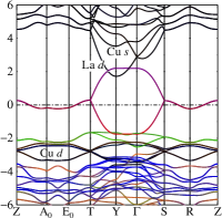
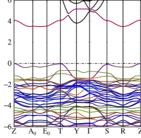
Figure 27: QSGW band structure (in eV) of nonmagnetic La₂CuO₄ (left) and antiferromagnetic LaCu₂O₄ (right). Colours reflect the orbital character of the bands as follows: Cu $d_{x^{2}{-}y^{2}}$ (red); Cu $d_{3z^{2}-1}$ (green), near $-$2 eV in QSGW; O-$p_{xy}$ (blue), between $-$3 eV and $-$5 eV in QSGW; O-$p_{z}$ (orange), between $-$3 eV and $-$5 eV in QSGW. The band near 3.3 eV at Y has significant Cu $s$ character, and it also admixes into the Cu $d_{x^{2}{-}y^{2}}$ near $E_{F}$.

The greatest failings appear in QSGW for systems where spin fluctuations are large. This is not surprising since the main many-body effect in GW are plasmons. GW has no diagrams in spin beyond the Fock exchange. When spin fluctuations become important, the first effect is to reduce the average moment [136, 137]. As they increase, states begin to lose their coherence: the band picture and QSGW both begin to break down. A good example of this is La₂CuO₄ (Fig. 27). Undoped La₂CuO₄ undergoes a paramagnetic to an antiferromagnetic insulator transition upon cooling below 325 K [138]. Fig. 27 shows QSGW calculations in the nonmagnetic state, and the antiferromagnetic one. Approximating the paramagnetic state by nonmagnetic state is an inadequate approximation, though it is often done. In this approximation La₂CuO₄ is predicted to be metallic, with a single Cu $d_{x^{2}-y^{2}}$ band crossing $E_{F}$. In the antiferromagnetic state La₂CuO₄ is found to be an insulator with a 3.5 eV bandgap. Experimentally La₂CuO₄ is an insulator with a gap $\sim$2 eV.

QSGW severely overestimates the optical gap in La₂CuO₄. There is a similar mismatch for CoO: the gap is overestimated by $\sim$2 eV in these cases, but not in NiO. Particularly telling is how for VO₂ nonmagnetic QSGW does describe the M1 phase very well when both V-V pairs dimerise [119], but not the M2 phase where only one of them does. (A gap opens up when M2 is calculated antiferromagnetically, but M2 is probably paramagnetic at room temperature.) M1 and M2 differ mainly through the V-V dimerisation, which suppresses spin fluctuations. As we will show elsewhere [126], including ladders considerably improves all of these antiferromagnetic insulators, but discrepancies remain particularly for La₂CuO₄. We believe this to be an artefact of the interaction between spin and charge fluctuations.

	$\Gamma$		M		Z
ARPES	9	$-$18	$-$22	$-$42	7	34
LDA	109	113	$-$204	$-$337	254	141
+DMFT	30	45	$-$110	$-$125	42	65
QSGW	41	44	$-$107	$-$202	131	56
+DMFT	1	10	$-$21	$-$40	10	32
SQS6	60	45	$-$52	$-$70	31	68

Table 7: $d_{xz}/d_{yz}$ and $d_{xy}$ QP levels (meV) near $E_{F}$ in tetragonal phase of FeSe (reference is the Fermi energy). LDA and QSGW data are calculated nonmagnetically; the line marked +DMFT following each is the result with DMFT added [139], as discussed in Sec. 5. Line SQS is a QSGW calculation in a ferrimagnetic SQS structure, as described in the text.

FeSe is a heavily studied superconductor with large spin fluctuations: it provides an excellent testbed to compare LDA and QSGW. Nonmagnetic calculations for LDA and QSGW are shown in Table 7. QSGW improves on the LDA, but discrepancies with ARPES are much larger than for, e.g. elemental Fe [115]. That LDA and QSGW should be different is readily seen from the $k$ dependence of the $Z$ factor, shown in Fig. 28. Local potentials such as the LDA cannot incorporate such an effect.

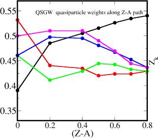
Figure 28: The orbitally resolved quasiparticle renormalization ($Z$) factors for FeSe Fe-3d orbitals along the high-symmetry Z-A line in tetragonal Brillouin zone; d_xy (black), d_yz (blue), d${}_{z^{2}}$ (green), d_xz (magenta), d${}_{x^{2}-y^{2}}$ (red).

Spin fluctuations are important, but QSGW does not adequately capture them. They can be incorporated in a mean-field manner by constructing a Special QuasiRandom Structure [140] with, in this case, three spin-up and three spin-down Fe atoms. Two magnetic solutions can be stabilised: a low-moment and high-moment solution. Quasiparticle spectra in the latter case are far removed from experiment, so we consider only the low-moment solution. The moments on each Fe site are different, with a range $|m|{=}0.2{\pm}0.15\mu_{B}$. The addition of magnetic terms shift QP levels closer to ARPES measurements, but a significant discrepancy with experiment remains. In Sec. 5 these results are revisited where local, high-order diagrams in spin are included.

These two systems show concretely how the shortcomings of GW become apparent when spin fluctuations are important. The simplest diagram beyond GW, the $T$ matrix, was first considered in an ab initio framework by Aryasetiawan and Karlsson [141]; more recently it was implemented in the spex code [142]. If spin fluctuations are not strong, as seems to be the case for Fe and Ni, such an approach seems to describe spin excitations fairly well, though comparisons with experiments are too sparse to draw any strong conclusions yet. For strong spin fluctuations, e.g. in La₂CuO₄ or other unconventional superconductors such as FeSe, it seems probable that many kinds of diagrams are needed, though the effective vertex entering into those diagrams is expected to be mostly local. Dynamical Mean Field Theory is ideally situated to address such cases; it is discussed in Sec. 5.

Our view is that QSGW with ladders in $W$ are sufficient for reliable description of susceptibilities within the charge channel, especially when ladders are included in the self-consistency cycle [102, 126] to make the QSGW $H_{0}$. In the spin channel DMFT contributes the dominant missing diagrams to the self-energy, and the susceptibilities can be reliably determined from local vertices, connected to $k$-dependent bubble diagrams.

5 DFT+DMFT and QSGW+DMFT

Hartree Fock and DFT are band structure theories: electrons are treated as though they are independent; in solids electron states are Bloch waves. GW includes correlations that go beyond the Bloch picture; still it is a perturbation around the Bloch description. In Landau Fermi-liquid theory, electrons are replaced by ‘quasi-particles’ which are adiabatically connected to the single-particle Bloch-wave representation of electrons. This, by construction, is a theory for excited states that adds perturbative corrections to the band picture. In Landau adiabatic theory electrons can have an effective mass, which is different from its free mass, and additionally, lifetime broadening effects far from the Fermi energy. One extreme case of this scenario is when the low-energy quasi-particle vanishes (without magnetic ordering) and the atomic-like, high-energy excitation emerges and effective mass at the Fermi energy tends to $\infty$. In effect, this is an emergent, non-adiabatic, feature where single-particle spectral weight flows to higher energies to conserve the total spectral weight and subsequently leads to suppression of low-energy quasi-particles. Popular rigid-band techniques [143, 144, 145, 146, 147, 148, 149, 150] would catch the physics of suppression of quasi-particles at Fermi energy, however, would fail to conserve the spectral weight since a dynamic self-energy ($\Sigma(\omega)$) is absent from those theories.

DMFT was formulated as an effective theory that smoothly interpolates between the Bloch-wave limit and atomic limit. It is formulated as a local impurity embedded self-consistently in a medium or bath, and was introduced in a seminal work by Metzner and Vollhardt [151] in late 80’s. Several other works from Mueller-Hartmann [152], Brandt and Mielsh [153], Jarrell et al. [154] and Georges et al. [155] helped to build a strong foundation for DMFT. The formulation and the implementation became popular through the seminal work by Georges et al. [156] and later emerged as a way to study strong correlations in real systems, supplementing an ab initio LDA framework by embedding a model Anderson impurity hamiltonian inside an LDA bath [157].

An implementation of DMFT has three components: the partitioning of the Hamiltonian into impurity + bath, a means to solve the impurity problem, and the bath-impurity self-consistency. The bath is essential because correlated states of interest have both atomic-like and Bloch-like properties with interesting low- and high- energy excitations. Through self-consistency the impurity feeds back on the bath, and ensures that all the symmetries of the entire system are preserved. In Questaal, QSGW or DFT can act as the bath. We have interfaces to two local solvers: the hybridisation expansion flavor of continuous time Quantum Monte Carlo (CT-QMC) from TRIQS [28] and the CT-QMC written by Kristjan Haule [27].

For the partitioning, some correlated subspace must be identified and this is done using projectors. Usually the subspace is derived from atomic-like $d$- or $f$-states of a transition metal or $f$ shell element. For projectors maximally-localised Wannier orbitals have been widely used  [158, 159]. We have so far adopted the projection into partial waves of a particular $\ell$ in an augmentation sphere [160]. There are strong reasons to prefer this scheme: the basis set is atom-centred and very localised with a definite $\ell$, which is the Hilbert space where the correlations are strong. The less localised the basis, the more it contains weakly correlated components (e.g. O-p states in transition metal oxides). Too much population of the correlated subspace with uncorrelated parts conflicts with the physical interpretation of separation of bath and interacting subspace and can reduce the reliability of the method [161]. Moreover, very localised basis functions have a much weaker energy-dependence. As a consequence, with a very local projector it is possible to construct an effective interaction over a wide energy window, reducing the frequency-dependence of the effective interaction, and essentially recovering the partial waves in augmentation spheres [17]. Partial waves closely resemble atomic orbitals, so solving a purely locally correlated Hamiltonian with the approximation of single-site DMFT (local self energy) is a good approximation.

The thorniest issue is how to construct the effective local Hamiltonian. It requires three related quantities: definition of the local Green’s function, an effective coulomb interaction $U$, which is partially screened by the bath, and the double counting (DC) correction.

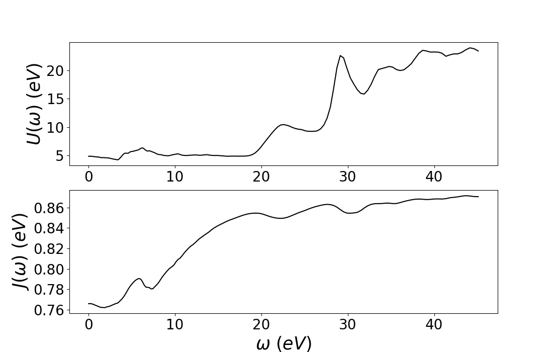
Figure 29: $U(\omega)$ and $J(\omega)$ computed using our c-RPA scheme for Ni 3d orbitals starting from a QSGW bath.

In a fully ab initio QSGW + DMFT theory, these quantities must be computed from the theory itself, but how to accomplish this is far from a settled issue. Questaal can estimate the Hubbard U and J using the constrained random-phase approximation [162] where the internal transitions between states included in the DMFT subspace are removed. A fully internally consistent theory requires a frequency-dependent $U(\omega)$, but available solvers can only solve the local impurity problem with such a U in the density-density channel. Haule’s prescription for excluding states in a large energy window partially mitigates this issue, since $U$ is closer to bare and nearly energy-independent [17]. (It makes another approximation, namely that not all the states excluded from screening are included in the impurity problem; these states are effectively treated only at the bath level.)

5.1 Questaal’s Implementation of DMFT

Questaal does not have its own DMFT solver. It has an interface to Haule’s CTQMC solver [27] and to the TRIQS library [28]. Haule’s CTQMC solver uses singular value decomposition (SVD) and TRIQS uses Legendre polynomial basis as compact representations for single-particle propagators.

A fully ab initio implementation is a work in progress, that will be reported on elsewhere. Within Questaal $U,J$ can be calculated within constrained RPA, following Ersoy et al. [163]. It has been tested on several materials; for instance, the Hubbard $U$ and Hund’s $J$ for Ni are shown in Fig. 29 which agrees well with Ref. [163]. The Hubbard U for FeSe using QSGW gives $U(0)=3.4$ eV, also close to what has been found in the literature [162]. In practical calculations today, we use a static $U$ and adopt the fully localised limit (FLL) for double counting (Sec.3.8).

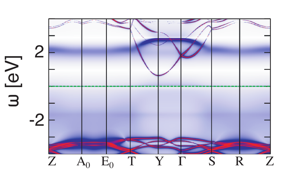
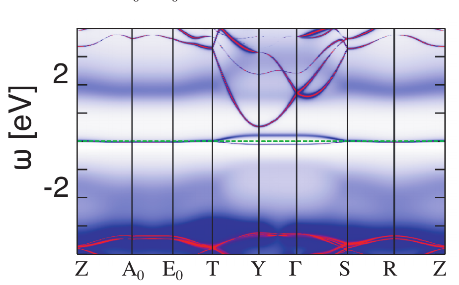
Figure 30: QSGW + DMFT spectral functions for La₂CuO₄ (left) and metallic QSGW + DMFT spectral functions for doped ($x$=0.12) La_2-xSr_xCuO₄ (right) which shows the classic three-peaked structure with upper and lower Hubbard bands at around $\pm$2 eV, and an almost dispersionless band at $E_{F}$.

We have used QSGW+DMFT to study single- and two- particle properties of the hole doped cuprate, La_2-xSr_xCuO₄. The parent compound at $x$=0 is a Mott insulator; while QSGW calculated non-magnetically leads to a metallic band structure, and an insulator with a wide gap when done antiferromagnetically (Fig. 27). The spins on the Cu in La₂CuO₄ fluctuate strongly and corresponding spin fluctuation diagrams are missing from QSGW. DMFT incorporates the local spin fluctuation diagrams with an exact solver (typically CTQMC), for the prescribed local Hamiltonian, and it can in principle, and indeed does, open a Mott gap [86, 17] (charge blocking without magnetic ordering). The five Cu-$3d$ partial waves in the augmentation spheres comprise the correlated subspace, and the $3d_{x^{2}-y^{2}}$ splits off to form the gap (Fig. 30), which is the paramamagnetic analogue to the antiferromagnetic QSGW band structure (Fig. 27). We solve the correlated impurity Hamiltonian in the Cu-$3d$ orbitals using the single-site CT-QMC solver within paramagnetic DMFT. Embedding local Green’s functions into the QSGW bath, we can compute the non-local Green’s functions dressed by the local DMFT self energy. They can be used to make spectral functions and the bubble diagrams entering into response functions (Sec. 6.3).

On doping, La_2-xSr_xCuO₄ undergoes a metal-insulator transition when $x$ is sufficiently large. At high temperatures, the $x$=0.12 system is known to be metallic. We recover a metallic solution in our QSGW+DMFT for $x$=0.12, using a virtual crystal approximation for $x$. We find the classical three peak spectral feature with atomic-like upper and lower Hubbard bands and a low energy incoherent quasi-particle peak at $E_{F}$ (Fig. 30). This structure is typical to strongly correlated metals in proximity of a localisation-delocalisation transition [156, 164]. Comparing with the insulating case at $x$=0, the spectral features for $x$=.12 has a natural explanation in the fact that spectral weight flows to low energies under doping.

Single-site DMFT incorporates the local spin fluctuation diagrams through a local self energy. It can not explain Fermi-arc features of weakly hole-doped cuprates and momentum-dependent suppression of electron pockets in de-twinned FeSe. In weakly hole-doped cuprates Fermi arc emerges, most likely, due to spin fluctuations which are longer ranged in nature and the corresponding diagrams are absent from single-site DMFT. Similarly, in FeSe, there are nematic fluctuations (which are inherently nonlocal), and the corresponding diagrams are absent from our theory. To incorporate such diagrams one needs to go beyond the single-site DMFT; cluster DMFT [165] or diagrammatic techniques like Dual Fermions [166].

6 Susceptibilities

Susceptibilities play a central role in many kinds of material properties. In the static limit they reduce to the second derivative of the total energy with respect to the corresponding perturbation. This section presents some general properties of linear susceptibilities, focusing on the transverse spin susceptibility $\chi^{+-}$, which is the magnetic analogue of the better known charge susceptibility. The formalism of the latter is very similar, but it is simpler as it concerns the response to a scalar potential. Also in the spin case, there is no analogue to the lowest order diagram (time-dependent Hartree approximation) in the charge case. To characterise the magnetic susceptibility beyond the noninteracting case requires a vertex such as the $T$ matrix [141].

Here we outline some general features; other sections explain how they are implemented in Questaal. The spin susceptibility relates the induced moment $\delta{\mathbf{m}}$ to a perturbation $\delta{\mathbf{B}}$:

$$\delta{\mathbf{m}}({{\mathbf{r}}},t)=-\int dt^{\prime}d^{3}r^{\prime}\chi({{\mathbf{r}}},{{\mathbf{r}}}^{\prime},t-t^{\prime}){\mathbf{B}}({{\mathbf{r}}}^{\prime},t^{\prime})$$ (178)

$\chi$ is a three-component tensor, $\chi^{\alpha\beta}$ with $\alpha$ and $\beta$ Cartesian coordinates. The charge susceptibility has the same form, only the perturbing potential is the scalar electric potential, which induces a (scalar) charge density. In general, there can be cross-coupling between spin and charge, so that the full $\chi$ is a $4{\times}4$ matrix connecting spin and magnetisation.

We restrict ourselves to linear perturbations around an equilibrium point, where the unperturbed system is time invariant. $\chi$ is a function only of the difference $t-t^{\prime}$, so its Fourier transform depends on a single frequency $\omega$. If in addition the reference system is in a periodic lattice, its Fourier transform space depends only on the difference in translation vectors, whose Fourier transform has a single ${{\mathbf{q}}}$ within the Brillouin zone with ${{\mathbf{r}}}$ and ${{\mathbf{r}}}^{\prime}$ limited to a unit cell. Denoting $\hat{\chi}({{\mathbf{q}}},{{\mathbf{r}}},{{\mathbf{r}}}^{\prime},\omega)$ as $\chi$ Fourier transformed in both space and time, $\hat{\chi}$ is typically what is measured by spectroscopy.

6.1 Spin Susceptibility

A perturbation causes the system to generate an internal field ${\mathbf{B}}_{\text{xc}}$, which adds to the total field, ${\mathbf{B}}_{\text{tot}}={\mathbf{B}}_{\text{ext}}+{\mathbf{B}}_{\text{xc}}$

$$\delta B_{\rm tot}^{\alpha}=\delta B_{\rm ext}^{\alpha}+\sum\nolimits_{\beta}\frac{\delta B_{\rm xc}^{\alpha}}{\delta m^{\beta}}\,\delta m^{\beta}$$ (179)

In collinear spin structures (all spins parallel to $z$), transverse and longitudinal components are decoupled. Moreover, by rotating from $(x,y)$ to $x^{+-}=x\pm iy$, the three-component $\chi$ becomes diagonal with transverse elements $\chi^{+-}$, $\chi^{-+}$, and longitudinal element $\chi^{zz}$. Eq. (178) also applies to the charge channel with the substitution ${\mathbf{B}}{\to}V$ and ${\mathbf{m}}{\to}n$, so that the full $\chi$ becomes a $4\times 4$ matrix, as noted above. In general $\chi^{zz}$ is coupled to the charge channel, while $\chi^{+-}$ and $\chi^{-+}$ are not. Also if the equilibrium system is nonmagnetic, $\chi^{+-}{=}\chi^{zz}$. In this work we are concerned only with $\chi^{+-}$ and the charge susceptibility $\chi^{Q}$, or alternatively the dielectric function.

The “magnetic” kernel $I_{\text{xc}}=\partial B_{xc}/{\partial m}$ is in general a function of $({{\mathbf{r}}},{{\mathbf{r}}}^{\prime},\omega)$, though it must satisfy a sum rule [110]. In many-body perturbation theory, the analogue of $I$ is the most challenging quantity to obtain, but in the adiabatic time-dependent LDA it is static and local, and is written in the transverse case as

$$I_{\rm xc}^{+-}({{\mathbf{r}}})=\frac{B_{xc}({{\mathbf{r}}})}{m({{\mathbf{r}}}^{\prime})}\delta({{\mathbf{r}}}-{{\mathbf{r}}}^{\prime})$$ (180)

Eq. (178) relates ${\mathbf{m}}$ to either ${\mathbf{B}}_{\text{ext}}$ or ${\mathbf{B}}_{\text{tot}}$

$$\delta{\mathbf{m}}=\chi_{0}\,\delta{\mathbf{B}}_{\text{tot}}=\chi\,\delta{\mathbf{B}}_{\text{ext}}$$ (181)

when $\chi_{0}$ and $\chi$ are the bare (noninteracting) and full susceptibilities, respectively. The preceding equations imply the relation

$$[\chi({{\mathbf{r}}},{{\mathbf{r}}}^{\prime},\omega)]^{-1}=[\chi_{0}({{\mathbf{r}}},{{\mathbf{r}}}^{\prime},\omega)]^{-1}-I_{\text{xc}}({{\mathbf{r}}},{{\mathbf{r}}}^{\prime},\omega)$$ (182)

The noninteracting susceptibility can be computed by linearising Dyson’s equation for the perturbation $\delta{\mathbf{B}}_{\text{ext}}$

$$-\chi_{0}^{+-}({{\mathbf{r}}}_{1},{{\mathbf{r}}}_{2},\omega)=G_{\uparrow}({{\mathbf{r}}}_{1},{{\mathbf{r}}}_{2},\omega)\otimes G_{\downarrow}({{\mathbf{r}}}_{1},{{\mathbf{r}}}_{2},-\omega)$$ (183)

$\otimes$ indicates frequency convolution: $f(\omega)\otimes g(\omega)=i/{2\pi}\int_{-\infty}^{\infty}{d\omega}f(\omega-\omega^{\prime})g(\omega^{\prime})$. We use $\downarrow$ for spin 1 and $\uparrow$ for spin 2. Similar equations with permutations of $\uparrow$ and $\downarrow$ may be written for the other components of $\chi_{0}$. In the Lehmann representation $\chi_{0}^{+-}$ involves the product of four eigenfunctions

$$\chi_{0}^{+-}({{\mathbf{q}}},{{\mathbf{r}}}_{1},{{\mathbf{r}}}_{2},\omega)=\\ \phantom{+}\sum^{\rm occ}_{{{\mathbf{k}}}n\downarrow}\sum^{\rm unocc}_{{{\mathbf{k}}}^{\prime}n^{\prime}\uparrow}\frac{\Psi_{{{\mathbf{k}}}n\downarrow}^{*}({{\mathbf{r}}}_{1})\Psi_{{{\mathbf{k}}}^{\prime}n^{\prime}\uparrow}({{\mathbf{r}}}_{1})\Psi_{{{\mathbf{k}}}^{\prime}n^{\prime}\uparrow}^{*}({{\mathbf{r}}}_{2})\Psi_{{{\mathbf{k}}}n\downarrow}({{\mathbf{r}}}_{2})}{\omega-(\epsilon_{{{\mathbf{k}}}^{\prime}n^{\prime}\uparrow}-\epsilon_{{{\mathbf{k}}}n\downarrow})+i\delta}\\ +\sum^{\rm unocc}_{{{\mathbf{k}}}n\downarrow}\sum^{\rm occ}_{{{\mathbf{k}}}^{\prime}n^{\prime}\uparrow}\frac{\Psi_{{{\mathbf{k}}}n\downarrow}^{*}({{\mathbf{r}}}_{1})\Psi_{{{\mathbf{k}}}^{\prime}n^{\prime}\uparrow}({{\mathbf{r}}}_{1})\Psi_{{{\mathbf{k}}}^{\prime}n^{\prime}\uparrow}^{*}({{\mathbf{r}}}_{2})\Psi_{{{\mathbf{k}}}n\downarrow}({{\mathbf{r}}}_{2})}{-\omega-(\epsilon_{{{\mathbf{k}}}n\downarrow}-\epsilon_{{{\mathbf{k}}}^{\prime}n^{\prime}\uparrow})+i\delta}\\$$ (184)

where ${{\mathbf{k}}}^{\prime}={{\mathbf{q}}}+{{\mathbf{k}}}$. We note in passing, that in a proper MBPT formulation of susceptibility, e.g. the T-matrix [141, 142], is a four-point quantity: $\chi$ is solved by a Bethe-Salpeter equation involving $W$ and a four-point analogue of Eq. (LABEL:generalchi01q), which at the end is contracted to two coordinates.

The Questaal code at present does not yet have a perturbative (T matrix) approach for the spin susceptibility, although one was recently reported in a QSGW framework [167]. It does have the ability to include the charge analogue of ladder diagrams to solve a Bethe-Salpeter equation for the dielectric function [116]. DMFT can also be used to build a two-particle Green’s function (or susceptibility), including all local diagrams, from which a local four-point vertex can be extracted that replaces $I$.

The first QSGW implementation of magnetic response functions [110] was designed for local moment systems, by which is meant systems with rigid spins (RSA): when perturbed by a transverse $\delta{\mathbf{B}}^{\perp}_{\text{ext}}$ ${\mathbf{m}}$ rotates rigidly without changing shape. (Archetypal examples are Fe, NiO, and MnAs [110].) In such a case the representation of $\chi^{+-}({{\mathbf{r}}},{{\mathbf{r}}}^{\prime},\omega)$ simplifies to

$$m({{\mathbf{r}}})\,\chi^{+-}(\omega)\,m({{\mathbf{r}}}^{\prime})$$ (185)

and $I$ can be completely determined by the sum rule [110], thus avoiding a diagrammatic calculation for it. This is Questaal’s present perturbative approach to computing $\chi$.

In the RSA $\chi^{+-}({{\mathbf{r}}},{{\mathbf{r}}}^{\prime},\omega)$ is discretised to a lattice model and can be written as $\chi^{+-}_{{{\mathbf{R}}},{{\mathbf{R}}}^{\prime}}(\omega)$. This makes it convenient to construct a Heisenberg model

$$H=\sum_{RR^{\prime}}J_{RR^{\prime}}\delta{\mathbf{m}}_{R}\delta{\mathbf{m}}_{R}^{\prime}$$ (186)

and extract $J_{RR^{\prime}}$ from $\chi$ as

$$J_{RR^{\prime}}=\frac{\delta^{2}E}{\delta{{\mathbf{m}}_{R}}\delta{{\mathbf{m}}_{R^{\prime}}}}=[\chi^{+-}_{{{\mathbf{R}}},{{\mathbf{R}}}^{\prime}}(\omega{=}0)]^{-1}$$ (187)

The $\delta{\mathbf{m}}$ are understood to be transverse to ${\mathbf{m}}_{R}$. Thus QSGW can be used to determine coefficients $J_{RR^{\prime}}$ entering into the Heisenberg model. This basic idea, with some enhancements, is what is described in Ref. [110].

6.1.1 Magnetic Exchange Interactions in the ASA

Sec. 6 presents general formulations of the spin and charge susceptibility. In the ASA, the static transverse susceptibility is implemented in the lmgf code in a formulation essentially similar to the rigid-spin approximation described there, with an additional “long-wave” approximation [168]

$$\chi({{\mathbf{q}}})\approx I\,\chi^{-1}({{\mathbf{q}}})\,I$$ (188)

Using the sum rule, $I$ need not be calculated but inferred from $\chi_{0}$.

It is possible to compute $\chi_{0}$ from the full Green’s function, Eq. (57). But lmgf implements the classic Lichtenstein formula [169], in which exchange parameters $J_{RR^{\prime}}$ are derived in terms of the auxiliary $g$ and the “magnetic force” theorem. This latter says that the change in total energy upon spin rotation simplifies to the change in eigenvalue sum; it is a special instance of the Hellmanm-Feynman theorem. It was realised sometime later [168] that the Lichtenstein formula is correct only in the $q{\to}0$ limit (the long-wave approximation), beginning to deviate at around $k{=}0.25{\cdot}2\pi/a$ in elemental 3$d$ magnets. In the notation of this paper, Lichtenstein’s formula reads

$${J^{\ell}}^{\bot}_{RR^{\prime}}=\frac{1}{{2\pi}}\int^{\varepsilon_{F}}{d\varepsilon}\,{\mathop{\rm Im}\nolimits}{\rm{Tr}}_{L}{\dots}$$

$${\delta P_{R\ell}\left({g_{RLR^{\prime}L^{\prime}}^{\uparrow}\,g_{R^{\prime}L^{\prime}RL}^{\downarrow}+g_{RLR^{\prime}L^{\prime}}^{\downarrow}\,g_{R^{\prime}L^{\prime}RL}^{\uparrow}}\right)\delta P_{R^{\prime}\ell^{\prime}}}$$ (189)

Questaal implements it for crystals, and for alloys within the CPA. See Refs. [49, 170, 171] for a detailed description.

6.1.2 Comparing QSGW and LDA Spin Response Functions

The GW code has an implementation of spin response functions within the rigid spin approximation as described Sec.6. This avoids direct calculation of the vertex, and is very simple, but is restricted to local-moment systems. Ref. [110] applied this approach to NiO, MnO and MnAs, with excellent results.

Questaal has the ability to compute spin waves (SWs) directly, or to extract parameters $J$ entering into the Heisenberg model, Eq. (186). One application — Mn_xGa_1-xAs alloys — are particularly instructive because they continue to attract interest as a spintronics material. Here we will compare the (ASA) Lichtenstein formula against full-potential, rigid-spin result using both LDA and QSGW Hamiltonians. Computing properties for random alloys of any $x$ is feasible within the ASA, via either the Lichtenstein formula or relaxing large structures using spin statics, Sec. 2.19. But a similar study is not feasible today in QSGW, so instead we consider four-atom Special QuasiRandom Structures [140] to simulate Mn_0.25Ga_0.75As and Mn_0.75Ga_0.25As, and also the $x{=}1$ case. Mn’s large local moment of around 4$\mu_{B}$ makes the approximations in Questaal’s QSGW magnetic response good ones.

DFT predicts Mn_xGa_1-xAs to become a spin glass when $x\,{\gtrsim}\,0.35$, though $T_{c}$ depends on what fraction of Mn go into interstitial sites, and how the Mn are ordered on the Ga sublattice. One application of the Questaal code was to show how Mn in alloys that favour ordering on the (201) orientation can optimise $T_{c}$ [172]. In the pure Zb-MnAs case, $x$=1, LDA predicts to be strongly antiferromagnetic, with negative spin wave frequencies everywhere in the Brillouin zone (left panel, Fig. 31). The figures show SWs calculated in the ASA using the Lichtenstein formula, Eq. (189). Its long-wave approximation should be accurate for small $q$, but it underestimates the strength of $J$ for large $q$ [168]. This is apparent in Fig. 31, comparing the LDA and Lichtenstein formulas.

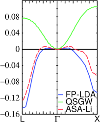
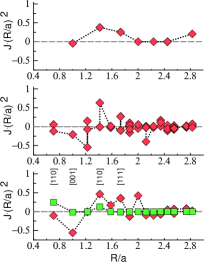
Figure 31: Left: spin waves in Zb-MnAs (eV) calculated in the GW code with QSGW potential (green) and LDA potential (blue), and also in the ASA-LDA with the Lichtenstein formula, Eq. (189). Right: Red diamonds show Heisenberg parameters $J$ Eq. (186) calculated in the ASA with Lichtenstein formula for a MnGa₃As₄ SQS structure (top), MnGa₂As₂ SQS structure (middle), and Zb-MnAs (bottom), as a function of neighbour distance. In the SQS structures, there can be inequivalent neighbours with the same connecting vector. LDA results calculated from the GW machinery look similar. Green squares: same parameters in ZB-MnAs using as QSGW potential. $J$ is in mRy.

This finding seems to contradict a measurement on a quantum dot of Zb-MnAs (Ref. [173]), which predicts it to be ferromagnetic. Indeed, QSGW calculations of the same system show that spin wave frequencies are everywhere positive (left panel, Fig. 31). $T_{c}$ based on Heisenberg parameters extracted magnon peaks in the SW spectrum is positive, of order 600K (somewhat larger than what Okabayashi observed).

Exchange parameters $J$ were extracted for three compositions, in LDA and for the pure MnAs case, in QSGW (right panel, Fig. 31). At 25% composition $J$ is still positive, but the nearest-neighbour $J$ is already very small. At 50%, $J$ is negative on average, and a spin glass is predicted. In pure Zb-MnAs, $J$ oscillate in sign with neighbour distance, but the nearest neighbours (particularly along [001]) are strongly antiferromagnetic, leading to negative frequencies in the SW spectrum. QSGW shows a marked contrast. Only the NN is important, with $J>0$. QSGW and LDA are so different because the LDA underestimates the exchange splitting between spin-up and spin-down $3d$ states, by $\sim$1 eV. This pushes the minority $d$ too close to $E_{F}$, and gives rise to long-range, antiferromagnetic interactions.

6.2 Optical Response Functions in Questaal

The linear optical response is described by the imaginary part of the dielectric response function $\epsilon_{2}(\omega)$ or equivalently the real part of the frequency dependent conductivity $\sigma_{1}(\omega)=-i\omega\epsilon_{2}(\omega)/4\pi$ at frequencies in the ultraviolet-visible (UV-VIS) range. From it one can obtain the real part $\epsilon_{1}(\omega)$ by the Kramers-Kronig relation and hence other relevant functions such as the complex index of refraction $\tilde{n}(\omega)=\sqrt{\epsilon_{1}(\omega)+i\epsilon_{2}(\omega)}=n(\omega)+i\kappa(\omega)$ with $\kappa(\omega)$ the extinction coefficient and $n(\omega)$ the real part of the index of refraction. The reflectivity $R(\omega)$ is then obtained via the Fresnel equations. For instance, the normal incidence reflectivity

$$R(\omega)=\left|\frac{\tilde{n}(\omega)-1}{\tilde{n}(\omega)+1}\right|^{2}$$ (190)

is a directly measurable quantity. The absorption coefficient

$$\alpha(\omega)=\frac{2\omega\kappa(\omega)}{c}=\frac{\omega\epsilon_{2}(\omega)}{n(\omega)c}$$ (191)

is measurable in transmission and spectroscopic ellipsometry allows one to measure directly $\epsilon_{1}(\omega)$ and $\epsilon_{2}(\omega)$.

There are several levels of theory at which one can obtain the optical dielectric function supported in the Questaal package. Typically we need the macroscopic dielectric function:

$${\epsilon_{M}}(\omega)={[\epsilon_{G{=}G^{\prime}{=}0}^{-1}({\mathbf{q}}\to 0,\omega)]^{-1}}$$ (192)

This is essentially obtained as a byproduct of the GW method (see Sec. 4). One way to obtain this limit is to take a small but finite ${{\mathbf{q}}}$ and use lmgw to obtain the plane wave matrix elements of the inverse dielectric function. The direction of the finite ${{\mathbf{q}}}$ then defines the specific component of $[\epsilon_{2}(\omega)]_{\alpha\alpha}$ which is actually a tensor. If one simply calculates instead

$$\epsilon_{G{=}G^{\prime}{=}0}({\mathbf{q}}\to 0,\omega)$$ (193)

one obtains the value without local-field corrections.

Alternatively, however, one can take the limit ${{\mathbf{q}}}\rightarrow 0$ analytically and arrive at the Adler-Wiser formula in the RPA,

$$[\epsilon_{2}(\omega)]_{\alpha\beta}=\frac{8\pi^{2}e^{2}}{\Omega\omega^{2}}\sum_{n}\sum_{n^{\prime}}\sum_{{\bf k}\in\text{BZ}}f_{n{\bf k}}(1-f_{n^{\prime}{\bf k}})\\ \times\langle\psi_{n{\bf k}}|v_{\alpha}|\psi_{n^{\prime}{\bf k}}\rangle\langle\psi_{n^{\prime}{\bf k}}|v_{\beta}|\psi_{n{\bf k}}\rangle\delta(\omega-\varepsilon_{n^{\prime}{\bf k}}+\varepsilon_{n{\bf k}})$$ (194)

Here $\Omega$ is the unit cell volume and $f_{n{\bf k}}$ are the occupation numbers, which in principle are given by the Fermi function at finite temperature but are in practice taken to be 0 or 1 for empty and occupied states respectively. The $v_{\alpha}$ are the components of the velocity operator ${\bf v}=\dot{\bf r}=(i/\hbar)[H,{\bf r}]$. For systems with at least orthorhombic symmetry the $\epsilon_{2}(\omega)$ tensor is diagonal in the Cartesian components. This well-known equation in the independent particle and long-wavelength form gives the $\epsilon_{2}(\omega)$ in terms of matrix-elements of the velocity operator and vertical interband transitions and can also be obtained from the Kubo formula for the optical conductivity. Within the all-electron methods (no non-local pseudopotentials) and if GW-self-energies are not included, the velocity matrix elements are equivalent to the momentum matrix elements ${\bf v}={\bf p}/m$ and can be obtained straightforwardly from the $\nabla$ operator matrix elements within the muffin-tin spheres and using a Fourier transform for the smooth part of the wave functions in the full-potential implementation. The matrix elements of the $\nabla$ operator between spherical harmonics times radial functions inside the muffin-tin spheres is obtained using the well-known gradient formula [174]; more generally, see Sec. 3.2 and Appendix D.

When the non-local self-energy operator or its Hermitian version are included, however, $(im/\hbar)[H,{\bf r}]$ is no longer equal to the momentum operator. To correct for this, the approximation proposed by Levine and Allan [175, 176] can be used, which consists in rescaling the matrix elements by a factor $(\varepsilon_{n^{\prime}{\bf k}}-\varepsilon_{n{\bf k}})/(\varepsilon^{LDA}_{n^{\prime}{\bf k}}-\varepsilon^{LDA}_{n{\bf k}})$. This is exact when the LDA and GW eigenfunctions are the same, and it works well in weakly correlated systems. However, it breaks down when correlations become strong, as in NiO. Questaal also has an approximate form for the proper nonlocal contribution to the velocity operator. As of this writing, it takes into account only intercell contributions. This approximation apparently does not work well in strongly correlated systems, and results with full matrix element will be reported in due course  [126].

The long-wave length approximation without local field (or excitonic) effects of $\varepsilon_{2}(\omega)$ can thus be obtained both in the ASA lm and the full-potential lmf codes and, when reading in the QSGW self-energy, can use the corrected quasiparticle energies rather than the Kohn-Sham eigenvalues. While approximate, it has the advantage that the $\mathbf{q}\rightarrow 0$ limit is taken analytically and that one can decompose the optical response in contributions from each occupied-empty band pair. By furthermore plotting vertical interband transition energies for any given pair, one can analyse where the bands are parallel and give their largest contribution to the joint density of states. This provides a way to relate the critical points or van-Hove singularities in the optical response to particular interband transitions. lmf and lm use this to enable decomposition into band-pair contributions if desired; it can also resolve contributions to $\epsilon$ by $k$.

The code also allows one to calculate dipole optical matrix elements between core states and valence or conduction band states and this can be used to model X-ray absorption (XAS) and emission (XES) spectroscopies. Furthermore, one can calculate Resonant X-ray Emission Spectroscopy (RXES) also known as Resonant Inelastic X-ray Scattering (RIXS) using the Kramers-Heisenberg equations [177]. The interesting point about this spectroscopy is that it allows to probe transitions between valence and conduction band states of the same angular momentum on a given site. In fact, let’s say one considers as X-ray edge the K-edge or $1s$ core level, then the RXES probes transitions between valence bands and conduction bands of $p$ angular momentum on the site of core hole that are in resonance with the difference of the absorbed and subsequently coherently emitted X-ray photon transitions from these conduction and valence states to the same core-hole. In optical measurements in the VIS-UV region, on the other hand, one probes only $\ell$ to $\ell\pm 1$ dipole allowed transitions. Using $p$-levels as core hole RIXS thus probes $d-d$ transitions, which often may be strongly influenced by many-body effects. The Kramers-Heisenberg formula assumes the wavevector of the X-ray can be neglected so that only direct transitions at the same k-point are allowed and within this approximation it allows one in principle to extract band-dispersions in a manner complementary to ARPES.

It was established 20 years ago that RPA approximation to the dielectric function can be dramatically improved by adding ladder diagrams via a Bethe-Salpeter equation [124, 125] (BSE) in simple $sp$ semiconductors. Traditionally the method is used by substituting GW eigenvalues for the DFT ones obtained from one-shot GW (Sec. 4). For simple $sp$ semiconductors where LDA and GW eigenfunctions are similar, this works well. It does not, however, when correlations become strong, e.g. in Cu₂O, where it was shown that $\epsilon(\omega)$ calculated from the BSE starting from a QSGW reference described the measured spectrum quite well [178]. Recently Cunningham et al. studied optics from BSE using QSGW as reference for a number of systems, and found very good agreement with experiment even in correlated systems such as NiO [116] and the monoclinic phase of VO₂ [119]. However, when spin fluctuations are large and QSGW does not describe the underlying band structure well, as in La₂CuO₄ (see Sec. 4.4), the description begins to break down. Recently Cunningham has added ladders to $W$ in the QSGW self-consistency cycle. This seems to dramatically improve on the description of $\epsilon(\omega)$, even in an extreme case such as La₂CuO₄. These capabilities are embedded in the standard Questaal distribution.

In the ASA code lm second harmonic generation coefficients can also be calculated but this portion of the code has not recently been updated to become applicable in the full-potential lmf implementation. The calculation of NLO coefficients is a bit more complex even within the long-wavelength independent particle approximation because of the need to include both intra- and inter-band transitions and disentangle them in a careful manner. The way to obtain divergence free expression was described in a series of papers by John Sipe and coworkers [179, 180, 181]. The version implemented in the code [182] uses Aversa’s length gauge formalism. The intra-band matrix elements ${\bf r}_{i}$ and inter-band ${\bf r}_{e}$ in this formalism are

$$\langle n{\bf k}|{\bf r}_{i}|m{\bf k}^{\prime}\rangle =\delta_{nm}[\delta({\bf k}-{\bf k}^{\prime})\xi_{nn}+i\nabla_{\bf k}\delta({\bf k}-{\bf k}^{\prime})]$$

$$\langle n{\bf k}|{\bf r}_{e}|m{\bf k}^{\prime}\rangle =(1-\delta_{nm})\delta({\bf k}-{\bf k}^{\prime})\xi_{nm}$$ (195)

with

$$\xi_{nm}\equiv\frac{(2\pi)^{3}i}{\Omega}\int_{\Omega}d^{3}r\,u_{n{\bf k}}^{*}({\bf r})\nabla_{\bf k}u_{m{\bf k}}({\bf r})$$ (196)

in which $\Omega$ is the volume of the unit cell and $u_{n{\bf k}}({\bf r})$ is the periodic part of the Bloch function. The $\xi_{nn}$ can be recognised to be a Berry connection. The manipulation of the matrix elements of ${\bf r}_{i}$ in commutators is non-trivial but described in detail in Aversa and Sipe [179]. An update of these parts of the code to incorporate them in lmf and to be made compatible with QSGW band structures as input is intended.

See also Sec. 6.3.

6.3 Response Functions within DMFT

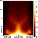
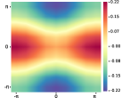
Figure 32: (left) Real part of $\chi(q,\omega{=}0)$ for La₂CuO₄ showing a dominant peak at q=($\pi,\pi$). (middle) Imaginary part of $\chi(q,\omega)$ (arbitrary units) for La_1.88Sr_0.12CuO₄ showing that spin fluctuations get gapped at ($\pi,\pi$) below 145 K. (right) Nodal superconducting gap structure for the hole-doped La₂CuO₄ showing d${}_{x^{2}-y^{2}}$ gap symmetry. The color bar shows the negative (in blue) and positive (in red) superconducting gap magnitudes in arbitrary units passing through node where the gap closes (in yellow).

With a converged self-energy, the CTQMC can sample the two-particle Green’s function [183] to obtain local spin and charge vertices. Finally, the non-local Bethe-Salpeter equations (BSE) in spin, charge and superconducting channels [183] can be solved from a local vertex and a non-local polarisation bubble in the respective channels. This allows us to compute the corresponding real [86] and imaginary part of susceptibilities [86, 184] in those channels. In Fig. (32) we show the real part of the spin susceptibilities in $x$=0 La_2-xSr_xCuO₄, adapted from Ref. [86]. There is a peak at q=($\pi,\pi$) suggesting dominant Néel anti-ferromagnetic spin fluctuations (Fig. 32).

We compute the imaginary part of the spin susceptibilities along the line ($h,k,l$) = (0,1/2,0)$-$(1,1/2,0) and find that the peak at (1/2,1/2,0) gets spin gapped (vanishing weight at $\omega$=0) when $x$=0.12 below a certain temperature, consistent with experimental observations [185]. Additionally, solving the BSE in the p-p superconducting channel we recover a superconducting gap function with d${}_{x^{2}-y^{2}}$ symmetry (right panel, Fig. 32). Our QSGW+DMFT implementation can be successfully applied to a wide range of systems; weakly correlated metals [115], strongly correlated metals [184] and correlated Mott insulators [86].

7 Towards a High-Fidelity Solution of the Many-Body Problem

Solving the many-electron problem with high-fidelity is a formidably difficult task. Our strategy to accomplish this relies on the following premises:

• many-body solutions are best framed around a non-interacting starting point, and we believe that QSGW is the best choice among them, by construction;

• charge fluctuations governed by long-range interactions, but they can be treated accurately with low-order perturbation theory; and

• spin fluctuations are governed mostly by single-site effective Hamiltonian (or action). The short-range interactions can be too strong to handle perturbatively, as can be seen by the non-analytic behaviour of one- and two-particle quantities, and their high degree of sensitivity to small perturbations, e.g. change in temperature. Nonlocal contributions are much weaker and can be treated in perturbation theory.

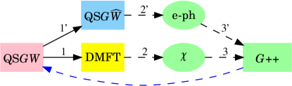
Figure 33: Questaal strategy for solving the many-electron problem.

Charge and spin fluctuations have very different characteristic energy scales: plasmon frequencies are typically of order 5 eV while typical magnon frequencies are of order 100 meV or less. As a conseqence they mutually interact weakly so that the self-energy is predominated by independent contributions from spin and charge channels. This is the premise of the Bose Factor Ansatz which has has been found to be effective in a DMFT framework [186].

We have framed a hierarchical strategy around these premises (Fig. 33). At the lowest level is QSGW, which depends only minimally on DFT. We think this is of central importance to frame a consistently reliable theory, for reasons we have pointed out in Sec. 4.1.

Referring to the figure, QSGW is adequate for many purposes. When not, there are two routes: a perturbative, nonlocal path $(1^{\prime},2^{\prime},3^{\prime})$ : low-order diagrams are added to $W$ to make $(W\to\widehat{W})$. To date we have added ladders to the charge channel; in progress is a project to add the electron-phonon interaction perturbatively [187], effectively adding another bosonic contribution to $W$. Also possible, but not yet accomplished in Questaal, is to add low order spin fluctuation diagrams such as the T matrix. All of them make a better $G$ ($G^{{+}{+}}$ in the Figure). The second path begins as nonperturbative, local path $(1)$. From a local interaction nonlocal susceptibilities can be constructed $(2)$. We have shown a few instances of this in Sec. 6.3, and the results are remarkably good in cases we have studied so far, e.g. Ref. [184]. Finally, the susceptibilities can be used to add a new diagrammatic contribution $(3)$ to $G$ ($G{{+}{+}}$). The simplest addition is Dual Fermions [166].

Perhaps more satisfactory would be to have a single, unified approach, for example the Diagrammatic Monte Carlo (DiagMC) method [188]. But it is formidably difficult to make this method work practically in real systems, because of the enormous time and memory costs that realistic (as opposed to model) Hamiltonians require. We think that the JPO basis alluded to in Sec. 3.12 is perhaps the most promising framework to realise DiagMC for realistic Hamiltonians. Even in such a case an optimal approach would likely closely resemble Fig. 33, but with some cross-linking between paths $(1)$ and $(1^{\prime})$, using a diagrammatic Monte Carlo solver only to include nonlocal diagrams beyond the RPA.

8 Software Aspects

The software package has a long history and has featured a high level of modularisation from its early days. The different parts interoperate through shared interfaces and file data formats.

The implementation is mainly in procedural Fortran 77. Fixes and improvements as well as new feature code uses modern Fortran features (f2008+) for convenience as well as improved reliability and interoperability. Despite f77’s shortcomings and questionable reputation, sound software engineering practices have been observed, there is (1) extensive code documentation in an uniform format, (2) almost no shared mutable state (i.e. common blocks or module variables); (3) action through side effect is avoided and data is passed through arguments, (4) unnecessary temporary data copies are avoided, (5) data structures are organised with performance in mind and most heavy number crunching is outsourced to performance libraries implementing the BLAS, LAPACK, FFTW3 APIs, (6) the code is written in an uniform style with consistent flow patterns. This practice has been extended through the use of modern version tracking and continuous integration pipelines incorporating regression, coverage and performance testing, and minimal style policy enforcement.

8.1 Release Policy

We use the popular distributed version tracking system git. The public online hosted repository is hooked to continuous integration pipelines executing the steps above on each push event. New features are developed in separate feature branches, if pushed to the public online repository, these are visible to all users. When judged safe and reasonably usable, feature branches are merged to the main development branch (“lm”). After extensive use, the development branch is merged to the release branch (“master”) and a new release is tagged with a numerical version in the format vmajor.minor.patchlevel. If/when issues are discovered and fixed the patchlevel is incremented in a new tag and the new commits are merged back to the development branch and from there to the feature branches. This approach reduces the maintenance burden significantly, however it does mean that once the minor version is incremented there are no more patches offered to the older versions and users are strongly encouraged to update to the latest version available. Since new developments are effectively done by interested users, and there is as of yet no contractual support offered, we feel this is a justified arrangement and in the long term offers users new features and improved performance with effectively close to no risk. The major version is only incremented when a very significant, possibly incompatible rewrite of core components or the input system has been performed.

New code and changes to existing code require: (1) coding standards pass; (2) regression tests suite pass (approximately 350 tests as of this writing); and (3) test coverage of at least 90% of code.

8.2 Parallelisation

The programmes of the package support multilevel parallelisation multiprocessing through the message passing interface (MPI) and simultaneous multithreading through performance libraries and (when necessary) manual OpenMP directives. The full-potential program uses multiprocessing mostly during the Brillouin zone sampling, outside of the $q$-loop the MPI processes cooperate on the local potential generation, only multithreading is available within the processing of each $q$-point. The empirical polarisable ion tight binding program offers more flexibility in this regard by allowing simultaneous assignment of groups of processes to each $q$-point as well as spreading different blocks of $q$-points over groups of processes [189]. A somewhat similar approach has been recently developed by Martin Lüders for the GW code. While it is available in a feature branch it is not yet considered production ready and has not been merged to the main branch. The GW code is fairly multithreaded and for systems of at least 15-20 atoms performs well on many-core wide vector architectures like Intel’s Xeon Phi family of processors (tested on x200, Knight’s Landing). A small but performance-critical part was also ported to Nvidia’s CUDA parallel platform and shows promising performance on hardware with good double precision floating point capabilities (for example Titan, P100, V100 compute cards). The polarisable ion tight binding program makes more extensive use of CUDA; it is described in [189].

To ease parallel IO, classic fortran binary files are being moved to HDF5 based data files. This also improves interoperability with various postprocessing environments because the HDF5 libraries offer bindings to a variety of popular programming languages.

8.3 Usability

Full-potential
blm	automatic input file generator
lmf	main band code
lmfa	free atom solver
lmfgwd	interface to GW
lmfdmft	interface to DMFT
Atomic sphere approximation
lm	ASA band code
lmgf	ASA crystal Green’s function code
lmpg	ASA principal layer Green’s function
lmstr	ASA structure constants
tbe	empirical tight-binding
Post-processing and utilities
fplot	a graphics package
pldos	a DOS postprocessor
plbnds	a bands postprocessor
lmchk	checks structure-related quantities
lmdos	assembles partial DOS
lmfgws	dynamical self-energy postprocessing
lmscell	supercell maker
mcx	a matrix calculator

Editors
lmf${|}$lm --rsedit	restart file
lm --popted	optics
lmf --wsig$\sim$edit	static $\Sigma_{0}$
lmfgws --sfuned	dynamic $\Sigma$
lmf --chimedit	magnetic susceptibility
lmscell --stack	superlattice

Table 8: Main executables in the Questaal suite.

An ordinary text command line is all one needs to be able to use the programmes from the package. The main executables (see Table 8) support a number of flags, notable among which is “--input”, it causes the full input understood by the executable to be printed together with default values and short documentation for each token. Another very valuable and possibly unique feature is the ability to override almost any input file value through the command line through the small embedded preprocessor which renders the input transparent internally (Fig. 34). A third is the suite of special-purpose editors (see Table). There is extensive documentation online together with many tutorials and ready made example script snippets. Users are encouraged to report issues and offer ideas through the online ticketing system and contribute improvements or fixes through pull requests or inline patches.

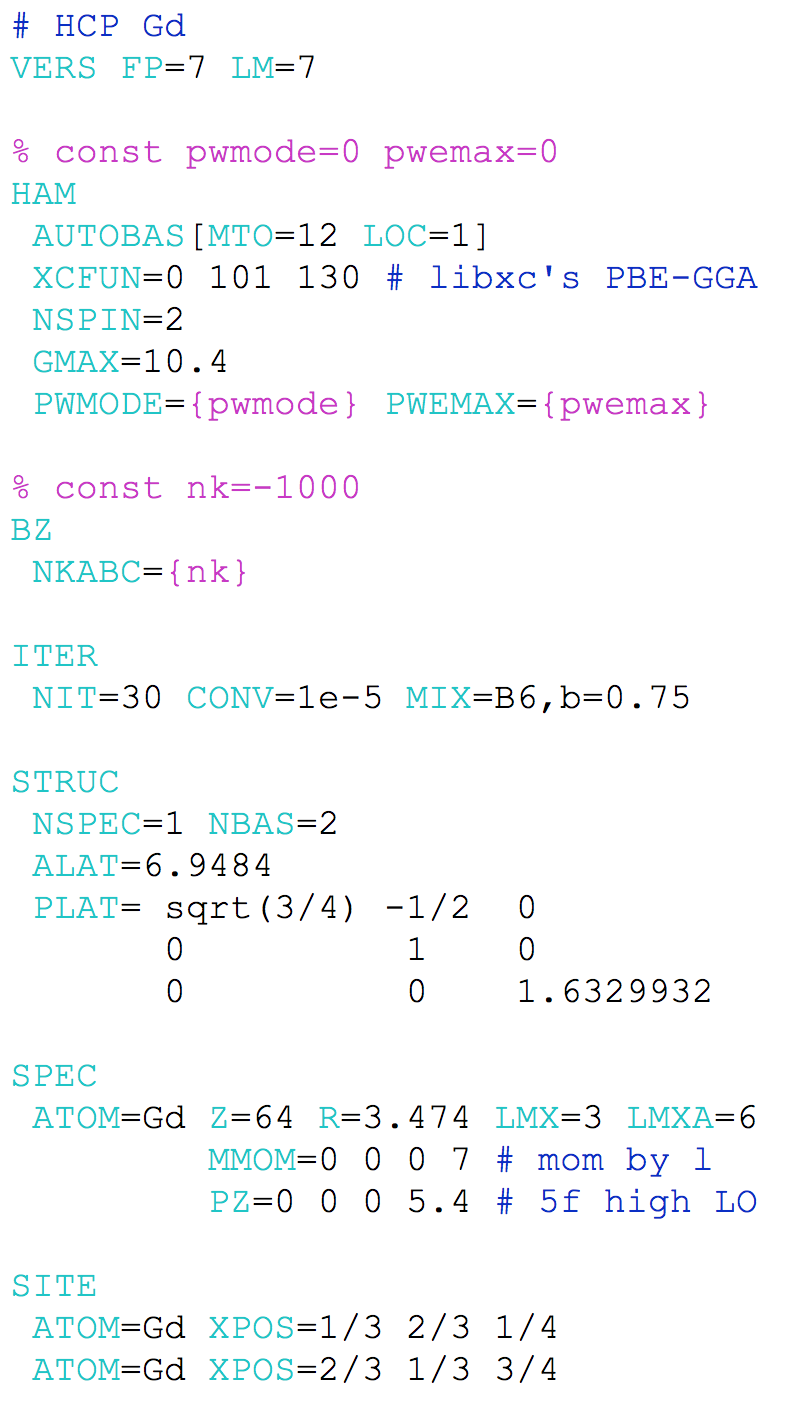
Figure 34: Basic input file: a full-potential GGA calculation for HCP Gd with 7$\mu_{B}$ $l=3$ starting moment. A preprocessor directive (nk) is used to specify the $k$-sampling, requesting 1000 points in the full Brillouin zone: the generated grid (12,12,7) has components corresponding to the relative BZ vector lengths. nk, like pwemax—which flags the inclusion of LAPW basis functions—can be changed from the command line. The LMTO basis is to be setup automatically, caused by the AUTOBAS token in the HAM (Hamiltonian) section.

8.4 Selected Publications from Questaal

In this section we point to original papers where new capabilities were developed within Questaal. Some the concepts are not original with Questaal, though many are:

• an early DFT calculation of the Schottky barrier height at a metal/semiconductor contact, showing the importance of screening at the interface [190];

• an early calculation of alloy phase diagrams combining statistical theory and DFT [191];

• a systematic technique for deriving force theorems within DFT [9];

• the first formulation of adiabatic spin dynamics within DFT [11] and its application to explain the Invar effect in permalloy [192];

• a formulation of self-consistent empirical tight-binding theory [29];

• a formulation of Electron Energy Loss Spectroscopy in DFT [193];

• the original description of Questaal’s full-potential method, Sec. 3 [31];

• the original description of Questaal’s all-electron GW approximation [194], and first calculation of RPA total energy in a solid [195];

• solution of the Boltzmann transport equation combined with DFT [196];

• the original formulation of Quasiparticle Self-Consistent GW [16], demonstration of its wide applicability [83], and a detailed description [84];

• Questaal’s implementation of nonequilibrium electron transport in nanosystems [14], and significant applications to magnetic transport [197, 22, 198, 24, 25];

• a fusion of genetic algorithms and exchange interactions to predict and optimise critical temperatures in multi-component systems [172];

• Dresselhaus terms calculated ab initio with high fidelity in zincblende semiconductors [107, 199, 109];

• first GW description of $4f$ systems, showing the tendency to overestimate splitting between occupied and unoccupied $f$ states  [135];

• spin wave theory within QSGW [110];

• prediction of Impact Ionisation rates with QSGW [113];

• the PMT method of Sec. 3.10 [54];

• a formulation of tunnelling transport within QSGW [112];

• effect of spin-orbit coupling on the QSGW self-energy [77];

• approximate description of transient absorption spectroscopy within QSGW [200];

• Questaal’s first application of QSGW+DMFT, showing the need to go beyond GW when spin fluctuations are important [115];

• addition of ladder diagrams to dielectric function [116];

• Fröhlich contribution to renormalisation of QSGW energy bands [128]; and

• first application of QSGW+DMFT+BSE for susceptibilities, Sec. 6.3 [86].

8.5 Distribution and Licensing

Historically the code has been distributed as a set of source tarballs, in addition registered users can git-clone our online repository. The code is distributed under the terms of the General Public license version 3. Contributions under a compatible license are welcome.

9 Conclusions

Questaal is a descendant of one of the early all-electron methods developed in Stuttgart. It has gradually evolved to its present form, but as no paper has been written for any of its stages the present work is intended to summarise much of this evolution. Our aim was to present the many expressions from classic works, combined with previously unpublished recent developments, in a unified way to show the connections between the parts.

We made an attempt to show Questaal’s strengths as well as its limits, within varying levels of theory. We think Questaal provides a very promising path to efficiently solve the electronic structure problem with high fidelity. It is unique in its potential to span such a wide range of properties and materials, and with varying levels of approximation.

10 Acknowledgements

Many people have contributed to the Questaal project. Much of the mathematics and basic algorithms in the lmf implementation were largely the work of Michael Methfessel. GW was formulated and implemented largely by Ferdi Aryasetiawan and Takao Kotani, and QSGW by Sergey Faleev. Martin Lüders wrote a parallel version of this code and was involved in some validation aspects. Derek Stewart wrote the original code for Landauer-Buttiker transport, and Faleev extended it to the nonequilibrium case. Pooya Azarhoosh improved on the optics and performed TAS studies. Alena Vishina redesigned the fully relativistic Dirac code, making it self-consistent. Herve Ness has redesigned significant parts of the layer Green’s function technique.

Brian Cunningham and Myrta Grüning added ladder diagrams to $W$, and Savio Laricchia is close to completing a QSGW-based approach to the electron-phonon interaction and related quantities. Both of these additions will have significant impact in the future. Also, many thanks to Kristjan Haule and Gabi Kotliar for helping us get started in DMFT, and to Ole Andersen for being the founder and inspiration for so many of the ideas behind Questaal.

Finally, many thanks to Andy Millis and the Simons Foundation, who enriched Questaal in fundamental ways, and to EPRSC which made it possible to become a community code (CCP9 flagship project: EP/M011631/1).

We gratefully acknowledge PRACE for awarding us access to SuperMUC at GCS@LRZ, Germany, the UK Materials and Molecular Modelling Hub for computational resources, which is partially funded by EPSRC (EP/P020194/1) and STFC Scientific Computing Department’s SCARF cluster (www.scarf.rl.ac.uk). J.J. acknowledges support under the CCP9 project “Computational Electronic Structure of Condensed Matter”, part of the Computational Science Centre for Research Communities (CoSeC).

Appendices

An augmentation radius is labelled by symbol $s$. Subscript $R$ is used to denote a site-dependent quantity, such as the augmentation radius $s_{R}$. When $R$ appears in a subscript of a function of ${{\mathbf{r}}}$ such as $H_{RL}({{\mathbf{r}}})$, it implies that ${{\mathbf{r}}}$ is relative to ${{\mathbf{R}}}$, i.e. $\mathbf{r-R}$. When a symbol refers to angular momentum, an upper case letter such as $L$, refers to both angular quantum number and magnetic quantum number parts, $\ell$ and $m$.

A Definition of Real and Spherical Harmonics

Where spherical harmonics are used, Questaal uses the same definitions as Jackson [201]:

$$Y_{\ell\,m}(\theta,\phi) =\left[\frac{(2\ell+1)(\ell-m)!}{4\pi(\ell+m)!}\right]^{\frac{1}{2}}P_{\ell}^{m}(\cos\theta){e^{im\phi}}$$ (A.1)

$$P_{\ell}^{m}(x) ={(-1)^{m}}\frac{(1-{x^{2}})^{m/2}}{2^{l}l!}\frac{d^{\ell+m}}{d{x^{\ell+m}}}{({x^{2}}-1)^{\ell}}$$ (A.2)

The $-m$ and $+m$ functions are related by [see Jackson (3.51) and (3.53)]

$$P_{\ell}^{-m}(x) =(-1)^{m}\frac{(\ell-m)!}{(\ell+m)!}P_{\ell}^{m}(x)$$ (A.3)

$$Y_{\ell,-m}(\hat{{{\mathbf{r}}}}) =(-1)^{m}Y^{*}_{\ell\,m}(\hat{{{\mathbf{r}}}})$$ (A.4)

Questaal mostly uses real harmonics $\text{Y}_{lm}$, which are related to the spherical harmonics as

$${\text{Y}_{\ell\,0}}(\hat{{{\mathbf{r}}}}) =\ Y_{\ell\,0}(\hat{{{\mathbf{r}}}})$$

$$\text{Y}_{\ell\,m}(\hat{{{\mathbf{r}}}}) =\frac{1}{\sqrt{2}}[(-1)^{m}{Y}_{\ell\,m}(\hat{{{\mathbf{r}}}})+{Y}_{\ell,-m}(\hat{{{\mathbf{r}}}})]$$

$$\text{Y}_{\ell,-m}(\hat{{{\mathbf{r}}}}) =\frac{1}{\sqrt{2}i}[{(-1)}^{m}{Y_{\ell\,m}}(\hat{{{\mathbf{r}}}})-Y_{\ell,-m}(\hat{{{\mathbf{r}}}})]$$ (A.5)

It also uses real harmonic polynomials, [note: substituted $l\to\ell$]

$$\mathcal{Y}_{{\ell}m}({{\mathbf{r}}})=r^{\ell}\text{Y}_{{\ell}m}(\hat{{{\mathbf{r}}}}),$$ (A.6)

which are real polynomials in $x$, $y$, and $z$.

The product of two spherical harmonic polynomials can be expanded as a linear combination of these functions in the same manner as ordinary ones

$$\text{Y}_{K}(\hat{{{\mathbf{r}}}})\text{Y}_{L}(\hat{{{\mathbf{r}}}}) =\sum_{M}C_{KLM}\text{Y}_{M}({\hat{{{\mathbf{r}}}}})$$ (A.7)

$$\mathcal{Y}_{K}({{{\mathbf{r}}}})\mathcal{Y}_{L}({{{\mathbf{r}}}}) =\sum_{M}C_{KLM}\,r^{k+\ell-m}\,\mathcal{Y}_{M}({{{{\mathbf{r}}}}})$$ (A.8)

The Gaunt coefficients $C_{KLM}$ are nonzero only when ${k+\ell-m}$ is an even integer, so the r.h.s. is also a polynomial in $(x,y,z)$.

Note also, from Eq. (A.6) it follows that if $\alpha$ is purely imaginary

$$\mathcal{Y}_{{\ell}m}(\alpha{{\mathbf{r}}})=(-1)^{l}\,\mathcal{Y}^{*}_{{\ell}m}(\alpha\mathbf{r})$$ (A.9)

It also follows from Eq. (A.6) and the discussion around Eq. (139) that

$$\nabla_{p}\mathcal{Y}_{L}({{{\mathbf{r}}}}) =(2\ell+1)\,\sum_{K}{{C}^{-}_{K{L};p}}\,\mathcal{Y}_{K}({{{{\mathbf{r}}}}})$$

$$-\nabla_{p}(r^{-2l-1}\mathcal{Y}_{L}({{{\mathbf{r}}}})) =(2\ell+1)\,\sum_{K}{{C}^{+}_{K{L};p}}\,\mathcal{Y}_{K}({{{{\mathbf{r}}}}})$$ (A.10)

for $p=1,2,3$. $r^{-2l-1}\mathcal{Y}_{L}({{{\mathbf{r}}}})$ and $\mathcal{Y}_{L}({{{\mathbf{r}}}})$ are ordinary Hankel and Bessel functions of energy zero. In the top (bottom) line, $k{=}\ell{+}1$ ($k{=}\ell{-}1$). Eqs. (A.10) may be taken as a definition of ${{C}^{(\pm)}_{K{L};p}}$. Similarly

$${{\mathbf{r}}}_{p}\mathcal{Y}_{L}({{\mathbf{r}}})=\sum_{K}\big{\{}{{C}^{(+)}_{K{L};p}}+{{C}^{(-)}_{K{L};p}}r^{2}\big{\}}\mathcal{Y}_{K}({{\mathbf{r}}})$$ (A.11)

$C^{(-)}$ is the transpose of $C^{(+)}$ :

$${{C}^{(+)}_{K{L};p}}={{C}^{(-)}_{L{K};p}}$$ (A.12)

but we keep them separate to distinguish terms that take $Y_{\ell,m}$ into $Y_{\ell+1,m^{\prime}}$ and those that map into $Y_{\ell-1,m^{\prime}}$.

B Definition of Hankel and Bessel Functions

To distinguish radial parts of spherical functions from solid versions, we denote spherical parts with subscript $\ell$, and solid functions with subscript $L$, which refers to both the $\ell$ and $m$ parts.

The Questaal codes generally follow Methfessel’s definitions for Hankel and Bessel functions. Writing $k{=}\sqrt{E}$ with $\text{Im}\,k{\geq}0$, they are related to standard spherical Neumann functions $n_{\ell}$ and Bessel functions $j_{\ell}$ as follows:

$$H_{L} =\mathcal{Y}_{L}(-\nabla)\,h_{0}(r)$$

$$=k^{\ell+1}n_{\ell}(kr)\text{Y}_{L},\quad E>0$$

$$=(ik)^{\ell+1}n_{\ell}(kr)\text{Y}_{L},\quad E<0$$

$$J_{L} =k^{-\ell}j_{\ell}(kr)\text{Y}_{L},\quad E>0$$

$$=(ik)^{-\ell}j_{\ell}(kr)\text{Y}_{L},\quad E<0$$

where

$$h_{0} =\text{Re}\,e^{ikr}/r\quad\text{and}\quad j_{0}=\sin(kr)/kr$$ (B.13)

$H_{L}$ and $J_{L}$ are real for any real energy, and structure constants Eq. (1) have the property $S_{KL}({{\mathbf{R}}})=S^{*}_{LK}(-{{\mathbf{R}}})$. They can generated from the $\ell{=}0$ functions using the operator $\mathcal{Y}_{L}(-\nabla)$; see, e.g. Eq. (117). The latter are useful for derivations and also practically, for instance, to express the gradient of $\nabla H_{L}$ as a linear combination of other $H_{L}$. Eq. (123) shows the explicit relation to the usual spherical Hankel function of the first kind, $h_{\ell}^{(1)}(z)$.

Spherical harmonics $Y_{L}$ can be substituted for the $\text{Y}_{L}$ in Eq. (B.13).

For historical reasons, Andersen made a different set of definitions, which are convenient for the ASA when $E$=0. In this paper we distinguish them from Questaal’s standard definitions Eq. (B.13) with a caret. For $E{\leq}0$ and $\kappa^{2}{=}-E$,

$$\hat{H}_{\ell}(\kappa,r) =-[(2\ell-1)!!(\kappa w)^{-\ell}]^{-1}(i\kappa w)h_{\ell}(\kappa r)$$

$$\xrightarrow{\kappa{\to}0}(w/r)^{\ell+1}$$

$$\hat{J}_{\ell}(\kappa,r) =(-1/2)[(2\ell-1)!!(\kappa w)^{-\ell}]j_{\ell}(\kappa r)$$

$$\xrightarrow{\kappa{\to}0}[2(2\ell+1)]^{-1}(r/w)^{\ell}$$ (B.14)

$w$ is a length scale which can be chosen arbitrarily (usually taken to be some average of the MT radii).

C Calculations in Real and Reciprocal Space

All of the formalism developed so far (with the exception of APWs) can apply to either real or reciprocal space. At present the Questaal codes work in reciprocal space, with the exception of lmpg (Sec. 2.14), which uses real space for the principal layer direction. The $k$ mesh is always a uniform mesh. Along any axis the user can specify whether the mesh has a point coinciding with $k$=0 or points that symmetrically straddle it.

When screened MTO’s are used, Bloch sums are formed directly from the short ranged orbitals. The standard lmf basis is not sufficiently short ranged, and Bloch sums are constructed with an Ewald technique. A Bloch sum of $\mathcal{H}_{L}$ is written as a sum over lattice vectors $\mathbf{R}$:

$${\mathcal{H}^{\mathbf{k}}_{L}(\varepsilon,\gamma;\mathbf{r})}=\sum\limits_{\mathbf{R}}{e^{i\mathbf{k}\cdot{\mathbf{R}}}\mathcal{H}_{L}(\varepsilon,\gamma;\mathbf{r-R})}={e^{i{\mathbf{k}}\cdot{\mathbf{r}}}}\sum\limits_{\mathbf{R}}{{e^{-i{\mathbf{k}}\cdot({\mathbf{r}}-{\mathbf{R}})}}\mathcal{H}_{L}(\varepsilon,\gamma;\mathbf{r-R})}$$

The latter sum is periodic in $\mathbf{R}$ and can be written as a Fourier series in the reciprocal lattice vectors $\mathbf{G}$

$$\sum\limits_{\mathbf{R}}{{e^{-i{\mathbf{k}}\cdot({\mathbf{r}}-{\mathbf{R}})}}\mathcal{H}_{L}(\varepsilon,\gamma;\mathbf{r-R})}=\frac{1}{V}\sum\limits_{\mathbf{G}}{{e^{i{\mathbf{G}}\cdot\mathbf{r}}}{\widehat{\mathcal{H}}_{L}}(\varepsilon,\gamma;{\mathbf{k+G}})}$$

so that the Bloch-summed $\mathcal{H}_{L}$ is

$${\mathcal{H}^{\mathbf{k}}_{L}(\varepsilon,\gamma;\mathbf{r})}=\frac{1}{V}\sum\limits_{\mathbf{G}}{{\widehat{\mathcal{H}}_{L}}(\varepsilon,\gamma;{\mathbf{k+G}}){e^{i({\mathbf{k+G}})\cdot\mathbf{r}}}}$$ (C.15)

$V$ is the volume of the unit cell.

D Matrix elements of Smooth Hankel Envelope Functions

This Appendix derives analytic expressions for matrix elements of the overlap, laplacian, gradient and position operators for a pair of functions $\mathcal{H}_{k_{2}L_{2}}(\varepsilon_{2},r_{s_{2}};{{{\mathbf{r}}}-\mathbf{R}_{2}})$ and $\mathcal{H}_{k_{1}L_{1}}(\varepsilon_{1},r_{s_{1}};{{{\mathbf{r}}}-\mathbf{R}_{1}})$, of the form Eq. (118). The strategy will be to use Parseval’s identity, Eq. (141), and evaluate the matrix elements of functions in reciprocal space. Analytic solutions can be obtained because products of functions $\widehat{\mathcal{H}}^{*}_{2}\widehat{\mathcal{H}}_{1}$ can be contracted to sums of functions of the same class, whose Fourier transform is known.

To begin with, consider matrix elements of the overlap and Laplacian operators. Since $\nabla^{2}\mathcal{H}_{kL}=\mathcal{H}_{k+1L}$, matrix elements of the Laplacian and overlap are different members of the same class. Using Eq. (116), (118) and (A.8), products of two $\widehat{\mathcal{H}}_{kL}(\mathbf{q})$ read as follows. To shorten the formulas the smoothing radius will be expressed in terms of $\gamma{=}r^{2}_{s}/4$.

$$\widehat{\mathcal{H}}^{*}_{1}\,\widehat{\mathcal{H}}_{2}=\left[\widehat{h}_{0}(\varepsilon_{1},\gamma_{1},q)\widehat{h}_{0}(\varepsilon_{2},\gamma_{2},q)\right]\Big{\{}(-q^{2})^{k_{1}+k_{2}}\,(-1)^{\ell_{1}}\,\mathcal{Y}_{L_{1}}(-i{{{\mathbf{q}}}})\,\mathcal{Y}_{L_{2}}(-i{{{\mathbf{q}}}})\Big{\}}\,e^{i{{\mathbf{q}}}\cdot\mathbf{R}_{1}}e^{-i{{\mathbf{q}}}\cdot\mathbf{R}_{2}}$$ (D.16)

The quantity in curly braces can be expanded into a linear combination of $\mathcal{Y}_{L}$ using Eq. (A.8),

$$(-q^{2})^{k_{1}+k_{2}}(-1)^{\ell_{1}}\,\mathcal{Y}_{L_{1}}(-i{{{\mathbf{q}}}})\,\mathcal{Y}_{L_{2}}(-i{{{\mathbf{q}}}}) =(-1)^{\ell_{1}}\sum_{M}C_{L_{1}L_{2}M}\,(-q^{2})^{k_{1}+k_{2}+(\ell_{1}+\ell_{2}-m)/2}\,\mathcal{Y}_{M}(-i{{{\mathbf{q}}}})$$ (D.17)

and the radial part in square brackets is similarly expanded

$$\widehat{h}_{0}(\varepsilon_{1},\gamma_{1},q)\widehat{h}_{0}(\varepsilon_{2},\gamma_{2},q) =\frac{{{{(4\pi)}^{2}}{e^{{\gamma_{1}}({\varepsilon_{1}}-{q^{2}})}e^{{\gamma_{2}}({\varepsilon_{2}}-{q^{2}})}}}}{{({\varepsilon_{1}}-{q^{2}})({\varepsilon_{2}}-{q^{2}})}}$$

$$=\frac{{{{(4\pi)}^{2}}}}{{{\varepsilon_{1}}-{\varepsilon_{2}}}}\left[{\frac{{{e^{{\gamma_{1}}({\varepsilon_{1}}-{\varepsilon_{2}})}}{e^{({\gamma_{1}}+{\gamma_{2}})({\varepsilon_{2}}-{q^{2}})}}}}{{{\varepsilon_{2}}-{q^{2}}}}-\frac{{{e^{{\gamma_{2}}({\varepsilon_{2}}-{\varepsilon_{1}})}}{e^{({\gamma_{2}}+{\gamma_{1}})({\varepsilon_{1}}-{q^{2}})}}}}{{{\varepsilon_{1}}-{q^{2}}}}}\right]$$

$$=\frac{{{{4\pi}}}}{{{\varepsilon_{1}}-{\varepsilon_{2}}}}\left[{{e^{{\gamma_{2}}({\varepsilon_{2}}-{\varepsilon_{1}})}}{\widehat{h}_{0}}({\varepsilon_{1}},\gamma,q)}-{e^{{\gamma_{1}}({\varepsilon_{1}}-{\varepsilon_{2}})}}{\widehat{h}_{0}}({\varepsilon_{2}},\gamma,q)\right]$$ (D.18)

$$\xrightarrow{\varepsilon_{2},\varepsilon_{1}\to\varepsilon}\frac{{(4\pi)}^{2}}{({\varepsilon_{2}}-{q^{2}})^{2}}{e^{({\gamma_{1}}+{\gamma_{2}})({\varepsilon}-{q^{2}})}}$$ (D.19)

$$\gamma ={\gamma_{1}}+{\gamma_{2}}.$$ (D.20)

When the factors in Eq. (D.16) are combined, the product is seen to be the Fourier transform of a linear combination of $\mathcal{H}_{kM}$ with smoothing radius given by $\gamma_{1}+\gamma_{2}$, at the connecting vector $\mathbf{R}_{1}-\mathbf{R}_{2}$. The overlap matrix can then be written

$$\begin{split}\left<\mathcal{H}_{k_{1}L_{1}}{\mathcal{H}}_{k_{2}L_{2}}\right>&=\int{{\mathcal{H}}^{*}_{k_{1}L_{1}}}(\varepsilon_{1},\gamma_{1};{{{\mathbf{r}}}}-{{{\mathbf{R}}}_{1}}){{\mathcal{H}}_{k_{2}L_{2}}}(\varepsilon_{2},\gamma_{2};{{{\mathbf{r}}}}-{{{\mathbf{R}}}_{2}})\,d^{3}r\\ &={4\pi}(-1)^{\ell_{1}}\sum_{M}C_{L_{1}L_{2}M}\Big{\{}{\frac{e^{-\gamma_{1}(\varepsilon_{2}-\varepsilon_{1})}}{\varepsilon_{2}-\varepsilon_{1}}{{\mathcal{H}}_{k^{\prime}M}}(\varepsilon_{2},\gamma;{{{\mathbf{R}}}})}-{\frac{e^{\gamma_{2}(\varepsilon_{2}-\varepsilon_{1})}}{\varepsilon_{2}-\varepsilon_{1}}{{\mathcal{H}}_{k^{\prime}M}}(\varepsilon_{1},\gamma;{{{\mathbf{R}}}})}\Big{\}}\\ k^{\prime}&=k_{1}+k_{2}+{(\ell_{1}+\ell_{2}-m)/2},\quad\gamma=\gamma_{1}+\gamma_{2},\quad{{\mathbf{R}}}={{{\mathbf{R}}}}_{1}-{{{\mathbf{R}}}}_{2}\end{split}$$ (D.21)

The case $\varepsilon_{1}=\varepsilon_{2}=\varepsilon$ must be handled specially. In that limit, the radial part simplifies to Eq. (D.19). This function is not contained in the ${\mathcal{H}}_{kL}$ pantheon, and a new function must be added

$$\begin{gathered}\widehat{\mathcal{W}}_{kL}({{\mathbf{q}}})={\widehat{w}_{0}(\varepsilon,r_{s};{q})}{(-iq)^{2k}}{\mathcal{Y}_{L}(-i{{{\mathbf{q}}}})}\\ \widehat{w}_{0}(\varepsilon,\gamma;{q})=\frac{4\pi}{(\varepsilon-q^{2})^{2}}e^{\gamma(\varepsilon-q^{2})}=\frac{-1}{(\varepsilon-q^{2})}\widehat{h}_{0}(\varepsilon,\gamma;{q})\end{gathered}$$ (D.24)

$\widehat{\mathcal{W}}_{kL}$ is closely related to the energy derivative of $\widehat{{\mathcal{H}}}_{kL}$. Differentiate Eq. (118), with respect to energy:

$$\begin{gathered}\widehat{\dot{\mathcal{H}}}_{kL}\equiv\frac{\partial{\widehat{\mathcal{H}}}_{kL}}{\partial\varepsilon}={\widehat{\mathcal{W}}}_{kL}+\gamma{\widehat{\mathcal{H}}}_{kL}\\ \text{which are generated from radial functions}\\ \widehat{\dot{h}}_{0}(\varepsilon,\gamma;{q})=\widehat{w}_{0}(\varepsilon,\gamma;{q})+\gamma\,\widehat{h}_{0}(\varepsilon,\gamma;{q})\end{gathered}$$ (D.28)

This provides a practical scheme to obtain ${\mathcal{W}}_{0L}$ in real space since analytic forms for ${\mathcal{H}}_{0L}$ and ${\dot{\mathcal{H}}}_{0L}$ are known (Eqs. (112) and (113)). To make $\mathcal{W}_{kL}$ for higher $k$ it is readily seen that

$$\mathcal{W}_{k+lL}({{\mathbf{r}}})=-\varepsilon\mathcal{W}_{kL}({{\mathbf{r}}})-\mathcal{H}_{kL}({{\mathbf{r}}})$$

Using Eq. (D.19) for the quantity in square brackets, Eq. (D.16), the resulting integral is

$$\begin{split}\int{{\mathcal{H}}^{*}_{k_{1}L_{1}}}(\varepsilon,\gamma_{1};{{{\mathbf{r}}}}-{{{\mathbf{R}}}_{1}}){{\mathcal{H}}_{k_{2}L_{2}}}(\varepsilon,\gamma_{2};{{{\mathbf{r}}}}-{{{\mathbf{R}}}_{2}})\,d^{3}r=&\\ {4\pi}(-1)^{\ell_{1}}\sum_{M}C_{L_{1}L_{2}M}{\ {{\mathcal{W}}_{k^{\prime}M}}(\varepsilon,\gamma;{{{\mathbf{R}}}})}\end{split}$$ (D.29)

where $k^{\prime}$, $\gamma$ and ${{\mathbf{R}}}$ the same as in Eq. (D.21). Note that Eq. (D.29) encompasses matrix elements between two generalized Gaussians, by virtue of Eq. (134), $H_{k+1L}(\varepsilon{=}0)=-{4\pi}G_{kL}$.

D.1 The momentum and position operators acting on a smooth Hankel function

Following the usual rules of Fourier transforms, the gradient operator $\nabla_{\mathbf{r}}$ and position operator $\mathbf{r}$ act in reciprocal space as follows. Use the definition Eqs. (116) and (118) with Eq. (A.11) to obtain

$$\begin{split}\nabla_{p}\,\mathcal{H}_{kL}(\varepsilon,\gamma;{{\mathbf{r}}})&=\frac{1}{(2\pi)^{3}}\int{\widehat{\mathcal{H}}_{kL}}(\varepsilon,\gamma;{{{\mathbf{q}}}})\,\nabla{{e^{i{\mathbf{q}}\cdot{{{\mathbf{r}}}}}}}\,{d^{3}}q\\ &=-\frac{1}{(2\pi)^{3}}\int{{e^{i{\mathbf{q}}\cdot{{{\mathbf{r}}}}}}}\,(-i{\mathbf{q}})\,\widehat{h}_{0}(\varepsilon,\gamma;q)\mathcal{Y}_{L}(-i{{\mathbf{q}}})\,{d^{3}}q\\ &=-\frac{1}{(2\pi)^{3}}\int{d^{3}}q\,{e^{i{\mathbf{q}}\cdot{{{\mathbf{r}}}}}}\sum_{M}\big{\{}{{C}^{(+)}_{M{L};p}}\widehat{{\mathcal{H}}}_{kM}({{\mathbf{q}}})+{{C}^{(-)}_{M{L};p}}{\mathcal{H}}_{k+1M}({{\mathbf{q}}})\big{\}}\\ &=-\sum_{M}\big{\{}{{C}^{(+)}_{M{L};p}}{{\mathcal{H}}}_{kM}({{\mathbf{r}}})+{{C}^{(-)}_{M{L};p}}{\mathcal{H}}_{k+1M}({{\mathbf{r}}})\big{\}}\end{split}$$ (D.30)

${C}^{(\pm)}_{M{L};p}$ has two nonzero elements for fixed $L;p$. The position operator is more complicated, and we restrict the derivation to $k{=}0$ case.

$${{\mathbf{r}}}\,\mathcal{H}_{0L}(\varepsilon,\gamma;{{\mathbf{r}}}) =\frac{1}{(2\pi)^{3}}\int{\widehat{\mathcal{H}}_{0L}}(\varepsilon,\gamma;{{{\mathbf{q}}}})\,\frac{\partial}{i\partial{\mathbf{q}}}{{e^{i{\mathbf{q}}\cdot{{{\mathbf{r}}}}}}}\,{d^{3}}q$$

$$=\frac{1}{(2\pi)^{3}}\int{{e^{i{\mathbf{q}}\cdot{{{\mathbf{r}}}}}}}\,[i{\nabla_{\mathbf{q}}}\widehat{h}_{0}(\varepsilon,\gamma;q)]\mathcal{Y}_{L}(-i{{\mathbf{q}}})+\widehat{h}_{0}(\varepsilon,\gamma;q)[i{\nabla_{\mathbf{q}}}\mathcal{Y}_{L}(-i{{\mathbf{q}}})]\,{d^{3}}q$$

The first term contains

$$[i{\nabla_{\mathbf{q}}}\widehat{h}_{0}(\varepsilon,\gamma;q)] =2i{\mathbf{q}}\,(\widehat{w}_{0}-\gamma\widehat{h}_{0})=2(-i{\mathbf{q}})\,\widehat{\dot{h}}_{0}$$

$$i{\nabla_{\mathbf{q}}}\widehat{h}_{0}(\varepsilon,\gamma;q)]{\mathcal{Y}_{L}(-i{{\mathbf{q}}})} =2\sum_{M}\big{\{}{{C}^{(+)}_{M{L};p}}{\widehat{\dot{\mathcal{H}}}_{0M}({{\mathbf{q}}})}+{{C}^{(-)}_{M{L};p}}{\widehat{\dot{\mathcal{H}}}_{1M}({{\mathbf{q}}})}\big{\}}$$

using Eq. (A.11). The second term follows directly from Eq. (A.10) to yield

$${{\mathbf{r}}}_{p}\,\mathcal{H}_{0L}(\varepsilon,\gamma;{{\mathbf{r}}}) =\sum_{M}\big{\{}{{C}^{(+)}_{M{L};p}}(2{\dot{\mathcal{H}}}_{0M}({{\mathbf{r}}}))+{{C}^{(-)}_{M{L};p}}({2{\dot{\mathcal{H}}}_{1M}({{\mathbf{r}}})}+(2\ell+1){{{\mathcal{H}}}_{0M}({{\mathbf{r}}})})\big{\}}$$ (D.31)

D.2 Matrix elements of position and gradient operators

Eq. (D.30) shows that $\nabla{{\mathcal{H}}_{kL}({{\mathbf{r}}})}$ generates a linear combination of the same family of ${{\mathcal{H}}_{kL}({{\mathbf{r}}})}$, evaluated at the vector connecting atom centres. Thus, matrix elements of the gradient operator are linear combinations of the same functions. A similar situation applies to matrix elements of ${{\mathbf{r}}}$, though they entail matrix elements of the overlap between ${{\mathcal{H}}_{kL}}$ and ${\dot{\mathcal{H}}}_{kL}$. These integrals can be evaluated in reciprocal space using Parseval’s identity, expanding $\widehat{\mathcal{H}}^{*}_{1}\,\widehat{\dot{\mathcal{H}}}_{2}$ analogously to Eq. (D.16). The radial part of this product can be expanded as:

$$\begin{gathered}\widehat{h}_{0}(\varepsilon_{1},\gamma_{1},q)\widehat{\dot{h}}_{0}(\varepsilon_{2},\gamma_{2},q)=\frac{{{{-(4\pi)}^{2}}{e^{{\gamma_{1}}({\varepsilon_{1}}-{q^{2}})}e^{{\gamma_{2}}({\varepsilon_{2}}-{q^{2}})}}}}{{({\varepsilon_{1}}-{q^{2}})({\varepsilon_{2}}-{q^{2}})^{2}}}+\gamma_{2}\,\widehat{h}_{0}(\varepsilon_{1},\gamma_{1},q)\widehat{{h}}_{0}(\varepsilon_{2},\gamma_{2},q)\\ =\frac{4\pi}{{\varepsilon_{1}-\varepsilon_{2}}}\bigg{\{}{{e^{\left(\varepsilon_{1}-\varepsilon_{2}\right)\,\gamma_{1}}}{\widehat{w}_{0}}({\varepsilon_{2}},\gamma,q)}+[{\gamma_{2}}+{{({\varepsilon_{1}}-{\varepsilon_{2}})}^{-1}}]\,{e^{-{\varepsilon_{2}}\,{\gamma_{1}}-{\varepsilon_{1}}\,{\gamma_{2}}}}\left(e^{\varepsilon_{1}\,\gamma}\,\widehat{h}_{0}(\varepsilon_{2},\gamma,q)-e^{\varepsilon_{2}\,\gamma}\,\widehat{h}_{0}(\varepsilon_{1},\gamma,q)\right)\bigg{\}}\end{gathered}$$ (D.34)

Substituting this radial function into the square brackets in Eq. (D.19), we obtain

$$\begin{split}\left<\mathcal{H}_{k_{1}L_{1}}\dot{\mathcal{H}}_{k_{2}L_{2}}\right>=&\int{{\mathcal{H}}^{*}_{k_{1}L_{1}}}(\varepsilon_{1},\gamma_{1};{{{\mathbf{r}}}}-{{{\mathbf{R}}}_{1}}){{\mathcal{\dot{H}}}_{k_{2}L_{2}}}(\varepsilon_{2},\gamma_{2};{{{\mathbf{r}}}}-{{{\mathbf{R}}}_{2}})\,d^{3}r\\ =&\frac{{4\pi}(-1)^{\ell_{1}}}{\varepsilon_{1}-\varepsilon_{2}}\sum_{M}C_{L_{1}L_{2}M}\times\bigg{\{}{{e^{\left(\varepsilon_{1}-\varepsilon_{2}\right)\,\gamma_{1}}}{{\mathcal{W}}_{k^{\prime}M}}(\varepsilon_{2})}\;+\\ &[{\gamma_{2}}+{{({\varepsilon_{1}}-{\varepsilon_{2}})}^{-1}}]\,{e^{-{\varepsilon_{2}}\,{\gamma_{1}}-{\varepsilon_{1}}\,{\gamma_{2}}}}\Big{(}e^{\varepsilon_{1}\,\gamma}\,{{\mathcal{H}}_{k^{\prime}M}}(\varepsilon_{2})-e^{\varepsilon_{2}\,\gamma}\,{{\mathcal{H}}_{k^{\prime}M}}(\varepsilon_{1})\Big{)}\bigg{\}}\end{split}$$ (D.35)

where ${\mathcal{W}_{k^{\prime}M}}$ and ${\mathcal{H}_{k^{\prime}M}}$ are evaluated with the same arguments $k^{\prime}$, $\gamma$ and ${{\mathbf{R}}}$ as in Eq. (D.21).

Combining Eqs. D.30, D.31, D.21 and D.35

$$\begin{split}\left<\mathcal{H}_{k_{1}L_{1}}\nabla_{p}\mathcal{H}_{k_{2}L_{2}}\right>&=\int{{\mathcal{H}}^{*}_{k_{1}L_{1}}}(\varepsilon_{1},\gamma_{1};{{{\mathbf{r}}}}-{{{\mathbf{R}}}_{1}})\nabla_{p}{{\mathcal{H}}_{k_{2}L_{2}}}(\varepsilon_{2},\gamma_{2};{{{\mathbf{r}}}}-{{{\mathbf{R}}}_{2}})\,d^{3}r\\ &=-\sum_{M}\big{\{}{{C}^{(+)}_{M{L_{2}};p}}\left<\mathcal{H}_{k_{1}L_{1}}\mathcal{H}_{k_{2}M}\right>+{{C}^{(-)}_{M{L};p}}\left<\mathcal{H}_{k_{1}L_{1}}\mathcal{H}_{k_{2}+1M}\right>\big{\}}\end{split}$$ (D.36)

$$\begin{split}\left<\mathcal{H}_{0L_{1}}({{{\mathbf{r}}}}-{{{\mathbf{R}}}_{2}})_{p}\mathcal{H}_{0L_{2}}\right>=\int{{\mathcal{H}}^{*}_{0L_{1}}}(\varepsilon_{1},\gamma_{1};{{{\mathbf{r}}}}-{{{\mathbf{R}}}_{1}})\left({{{\mathbf{r}}}}-{{{\mathbf{R}}}_{2}}\right)_{p}{{\mathcal{H}}_{0L_{2}}}(\varepsilon_{2},\gamma_{2};{{{\mathbf{r}}}}-{{{\mathbf{R}}}_{2}})\,d^{3}r\\ =\sum_{M}\Big{\{}{{C}^{(+)}_{M{L_{2}};p}}2\left<\mathcal{H}_{0L_{1}}\dot{\mathcal{H}}_{0M}\right>+{{C}^{(-)}_{M{L};p}}\left(2\left<\mathcal{H}_{0L_{1}}\dot{\mathcal{H}}_{1M}\right>+(2\ell_{2}+1)\left<\mathcal{H}_{0L_{1}}\mathcal{H}_{0M}\right>\right)\Big{\}}\end{split}$$ (D.37)

References

- [1] J. Korringa, Phys. Rep. 238 (1994) 341–360. doi:10.1016/0370-1573(94)90122-8.
- [2] C. Herring, Phys. Rev. 57 (1940) 1169–1177. doi:10.1103/PhysRev.57.1169.
- [3] J. C. Slater, Phys. Rev. 51 (1937) 846–851. doi:10.1103/PhysRev.51.846.
- [4] P. E. Blöchl, Phys. Rev. B 50 (1994) 17953–17979. doi:10.1103/PhysRevB.50.17953.
- [5] O. K. Andersen, Phys. Rev. B 12 (1975) 3060–3083. doi:10.1103/PhysRevB.12.3060.
- [6] K. Lejaeghere, G. Bihlmayer, T. Bjorkman, P. Blaha, S. Blugel, V. Blum, D. Caliste, I. E. Castelli, S. J. Clark, A. Dal Corso, S. de Gironcoli, T. Deutsch, J. K. Dewhurst, I. Di Marco, C. Draxl, M. Duak, O. Eriksson, J. A. Flores-Livas, K. F. Garrity, L. Genovese, P. Giannozzi, M. Giantomassi, S. Goedecker, X. Gonze, O. Granas, E. K. U. Gross, A. Gulans, F. Gygi, D. R. Hamann, P. J. Hasnip, N. A. W. Holzwarth, D. Iuan, D. B. Jochym, F. Jollet, D. Jones, G. Kresse, K. Koepernik, E. Kucukbenli, Y. O. Kvashnin, I. L. M. Locht, S. Lubeck, M. Marsman, N. Marzari, U. Nitzsche, L. Nordstrom, T. Ozaki, L. Paulatto, C. J. Pickard, W. Poelmans, M. I. J. Probert, K. Refson, M. Richter, G.-M. Rignanese, S. Saha, M. Scheffler, M. Schlipf, K. Schwarz, S. Sharma, F. Tavazza, P. Thunstrom, A. Tkatchenko, M. Torrent, D. Vanderbilt, M. J. van Setten, V. Van Speybroeck, J. M. Wills, J. R. Yates, G.-X. Zhang, S. Cottenier, Science 351 (2016) aad3000–aad3000. doi:10.1126/science.aad3000.
- [7] M. Methfessel, D. Hennig, M. Scheffler, Phys. Rev. B 46 (1992) 4816–4829. doi:10.1103/PhysRevB.46.4816.
- [8] A. I. Liechtenstein, I. I. Mazin, C. O. Rodriguez, O. Jepsen, O. K. Andersen, M. Methfessel, Phys. Rev. B 44 (1991) 5388–5391. doi:10.1103/PhysRevB.44.5388.
- [9] M. Methfessel, M. van Schilfgaarde, M. Scheffler, Phys. Rev. Lett. 70 (1993) 29–32. doi:10.1103/PhysRevLett.70.29.
- [10] M. I. Katsnelson, V. P. Antropov, M. van Schilfgaarde, B. N. Harmon, JETP Lett. 62 (1995) 439–443.
- [11] V. P. Antropov, M. I. Katsnelson, M. van Schilfgaarde, B. N. Harmon, Phys. Rev. Lett. 75 (1995) 729–732. doi:10.1103/PhysRevLett.75.729.
- [12] T. Kotani, H. Akai, Phys. Rev. B 54 (1996) 16502–16514. doi:10.1103/PhysRevB.54.16502.
- [13] F. Aryasetiawan, O. Gunnarsson, Phys. Rev. Lett. 74 (1995) 3221–3224. doi:10.1103/PhysRevLett.74.3221.
- [14] S. V. Faleev, F. Léonard, D. A. Stewart, M. van Schilfgaarde, Phys. Rev. B 71 (2005) 195422. doi:10.1103/PhysRevB.71.195422.
- [15] T. Kotani, M. van Schilfgaarde, Solid State Commun. 121 (2002) 461–465. doi:10.1016/S0038-1098(02)00028-5.
- [16] S. V. Faleev, M. van Schilfgaarde, T. Kotani, Phys. Rev. Lett. 93 (2004) 126406. doi:10.1103/PhysRevLett.93.126406.
- [17] S. Choi, A. Kutepov, K. Haule, M. van Schilfgaarde, G. Kotliar, npj Quantum Mater. 1 (2016) 16001. doi:10.1038/npjquantmats.2016.1.
- [18] O. K. Andersen, O. Jepsen, Phys. Rev. Lett. 53 (1984) 2571–2574. doi:10.1103/PhysRevLett.53.2571.
- [19] F. Caruso, P. Rinke, X. Ren, A. Rubio, M. Scheffler, Phys. Rev. B 88 (2013) 075105. doi:10.1103/PhysRevB.88.075105.
- [20] M. J. van Setten, F. Weigend, F. Evers, J. Chem. Theory Comput. 9 (2013) 232–246. doi:10.1021/ct300648t.
- [21] M. A. Marques, M. J. Oliveira, T. Burnus, Comput. Phys. Commun. 183 (2012) 2272–2281. doi:10.1016/j.cpc.2012.05.007.
- [22] A. N. Chantis, K. D. Belashchenko, E. Y. Tsymbal, M. van Schilfgaarde, Phys. Rev. Lett. 98 (2007) 046601. doi:10.1103/PhysRevLett.98.046601.
- [23] A. N. Chantis, K. D. Belashchenko, D. L. Smith, E. Y. Tsymbal, M. van Schilfgaarde, R. C. Albers, Phys. Rev. Lett. 99 (2007) 196603. doi:10.1103/PhysRevLett.99.196603.
- [24] K. D. Belashchenko, A. A. Kovalev, M. van Schilfgaarde, Phys. Rev. Lett. 117 (2016) 207204. doi:10.1103/PhysRevLett.117.207204.
- [25] K. D. Belashchenko, A. A. Kovalev, M. van Schilfgaarde, Phys. Rev. Mater. 3 (2019) 011401. doi:10.1103/PhysRevMaterials.3.011401.
- [26] F. Aryasetiawan, Phys. Rev. B 46 (1992) 13051–13064. doi:10.1103/PhysRevB.46.13051.
- [27] K. Haule, Phys. Rev. B 75 (2007) 155113. doi:10.1103/PhysRevB.75.155113.
- [28] O. Parcollet, M. Ferrero, T. Ayral, H. Hafermann, I. Krivenko, L. Messio, P. Seth, Comput. Phys. Commun. 196 (2015) 398–415. doi:10.1016/j.cpc.2015.04.023.
- [29] M. W. Finnis, A. T. Paxton, M. Methfessel, M. van Schilfgaarde, Phys. Rev. Lett. 81 (1998) 5149–5152. doi:10.1103/PhysRevLett.81.5149.
- [30] M. W. Finnis, Interatomic forces in condensed matter, Oxford University Press, Oxford, 2003.
- [31] M. Methfessel, M. van Schilfgaarde, R. A. Casali, in: H. Dreyssé (Ed.), Electronic structure and physical properties of solids: the uses of the LMTO method, no. 535 in Lecture notes in physics, Springer, Berlin, 2000, p. 114.
- [32] O. Gunnarsson, O. Jepsen, O. K. Andersen, Phys. Rev. B 27 (1983) 7144–7168. doi:10.1103/PhysRevB.27.7144.
- [33] O. K. Andersen, T. Saha-Dasgupta, R. W. Tank, G. K. C. Arcangeli, O. Jepsen, G. Krier, in: H. Dreyssé (Ed.), Electronic structure and physical properties of solids: the uses of the LMTO method, no. 535 in Lecture notes in physics, Springer, Berlin, 2000, p. 3.
- [34] O. K. Andersen, A. V. Postnikov, S. Y. Savrasov, in: W. H. Butler, P. H. Dederichs, A. Gonis, R. L. Weaver (Eds.), Applications of Multiple Scattering Theory to Materials Science, Vol. 253, Materials Research Society, Pittsburgh, 1992, pp. 37–70.
- [35] O. K. Andersen, Z. Pawlowska, O. Jepsen, Phys. Rev. B 34 (1986) 5253–5269. doi:10.1103/PhysRevB.34.5253.
- [36] M. van Schilfgaarde, W. R. L. Lambrecht, in: L. Colombo, A. Gonis, P. Turchi (Eds.), Tight-binding approach to Computational Materials Science, Vol. 491 of Lecture Notes in Physics, Springer, Berlin, 1998, p. 137.
- [37] M. P. L. Sancho, J. M. L. Sancho, J. Rubio, J. Phys. F 15 (1985) 851–858. doi:10.1088/0305-4608/15/4/009.
- [38] A.-B. Chen, Y.-M. Lai-Hsu, W. Chen, Phys. Rev. B 39 (1989) 923–929. doi:10.1103/PhysRevB.39.923.
- [39] A. K. Rajagopal, J. Callaway, Phys. Rev. B 7 (1973) 1912–1919. doi:10.1103/PhysRevB.7.1912.
- [40] G. Vignale, M. Rasolt, Phys. Rev. Lett. 59 (1987) 2360–2363. doi:10.1103/PhysRevLett.59.2360.
- [41] G. Vignale, M. Rasolt, Phys. Rev. B 37 (1988) 10685–10696. doi:10.1103/PhysRevB.37.10685.
- [42] H. Ebert, J. Phys. Condens. Matter. 1 (1989) 9111–9116. doi:10.1088/0953-8984/1/46/005.
- [43] I. Turek, V. Drchal, J. Kudrnovský, M. S̆ob, P. Weinberger, Electronic Structure of Disordered Alloys, Surfaces and Interfaces, Springer, Boston, 1997.
- [44] R. Feder, F. Rosicky, B. Ackermann, Z. Phys. B 52 (1983) 31–36. doi:10.1007/BF01305895.
- [45] J. Kudrnovský, V. Drchal, Phys. Rev. B 41 (1990) 7515–7528. doi:10.1103/PhysRevB.41.7515.
- [46] A. Devonport, A. Vishina, R. Singh, M. Edwards, K. Zheng, J. Domenico, N. Rizzo, C. Kopas, M. van Schilfgaarde, N. Newman, J. Magn. Magn. Mater. 460 (2018) 193–202. doi:10.1016/j.jmmm.2018.03.054.
- [47] V. Alena, Fully relativistic green’s functions method, Ph.D. thesis, Kings College London (2019).
- [48] M. Abd El Qader, R. K. Singh, S. N. Galvin, L. Yu, J. M. Rowell, N. Newman, Appl. Phys. Lett. 104 (2014) 022602. doi:10.1063/1.4862195.
- [49] V. P. Antropov, M. I. Katsnelson, B. N. Harmon, M. van Schilfgaarde, D. Kusnezov, Phys. Rev. B 54 (1996) 1019–1035. doi:10.1103/PhysRevB.54.1019.
- [50] M. van Schilfgaarde, I. A. Abrikosov, B. Johansson, Nature 400 (1999) 46–49. doi:10.1038/21848.
- [51] A. Bulgac, D. Kusnezov, Phys. Rev. A 42 (1990) 5045–5048. doi:10.1103/PhysRevA.42.5045.
- [52] T. Kotani, H. Kino, H. Akai, J. Phys. Soc. Jpn. 84 (2015) 034702. doi:10.7566/JPSJ.84.034702.
- [53] E. Bott, M. Methfessel, W. Krabs, P. C. Schmidt, J. Math. Phys. 39 (1998) 3393–3425. doi:10.1063/1.532437.
- [54] T. Kotani, M. van Schilfgaarde, Phys. Rev. B 81 (2010) 125117. doi:10.1103/PhysRevB.81.125117.
- [55] J. M. Soler, A. R. Williams, Phys. Rev. B 40 (1989) 1560–1564. doi:10.1103/PhysRevB.40.1560.
- [56] M. van Schilfgaarde, T. Kotani, S. V. Faleev, Phys. Rev. B 74 (2006) 245125. doi:10.1103/PhysRevB.74.245125.
- [57] D. J. Singh, L. Nordström, Planewaves, Pseudopotentials and the LAPW Method, Second Edition, Springer, Berlin, 2006.
- [58] J. Kunes̆, P. Novák, R. Schmid, P. Blaha, K. Schwarz, Phys. Rev. B 64 (2001) 153102. doi:10.1103/PhysRevB.64.153102.
- [59] C. Friedrich, M. C. Müller, S. Blügel, Phys. Rev. B 83 (2011) 081101. doi:10.1103/PhysRevB.83.081101.
- [60] H. Jiang, P. Blaha, Phys. Rev. B 93 (2016) 115203. doi:10.1103/PhysRevB.93.115203.
- [61] J. Harris, Phys. Rev. B 31 (1985) 1770–1779. doi:10.1103/PhysRevB.31.1770.
- [62] W. M. C. Foulkes, R. Haydock, Phys. Rev. B 39 (1989) 12520–12536. doi:10.1103/PhysRevB.39.12520.
- [63] V. I. Anisimov, J. Zaanen, O. K. Andersen, Phys. Rev. B 44 (1991) 943–954. doi:10.1103/PhysRevB.44.943.
- [64] V. I. Anisimov, I. V. Solovyev, M. A. Korotin, M. T. Czyżyk, G. A. Sawatzky, Phys. Rev. B 48 (1993) 16929–16934. doi:10.1103/PhysRevB.48.16929.
- [65] V. I. Anisimov, F. Aryasetiawan, A. I. Lichtenstein, J. Phys. Condens. Matter. 9 (1997) 767–808. doi:10.1088/0953-8984/9/4/002.
- [66] A. I. Liechtenstein, V. I. Anisimov, J. Zaanen, Phys. Rev. B 52 (1995) R5467–R5470. doi:10.1103/PhysRevB.52.R5467.
- [67] M. T. Czyżyk, G. A. Sawatzky, Phys. Rev. B 49 (1994) 14211–14228. doi:10.1103/PhysRevB.49.14211.
- [68] A. G. Petukhov, I. I. Mazin, L. Chioncel, A. I. Lichtenstein, Phys. Rev. B 67 (2003) 153106. doi:10.1103/PhysRevB.67.153106.
- [69] V. I. Anisimov, O. Gunnarsson, Phys. Rev. B 43 (1991) 7570–7574. doi:10.1103/PhysRevB.43.7570.
- [70] M. Cococcioni, S. de Gironcoli, Phys. Rev. B 71 (2005) 035105. doi:10.1103/PhysRevB.71.035105.
- [71] E. U. Condon, G. H. Shortley, The Theory of Atomic Spectra, Cambridge University Press, Cambridge, 1953.
- [72] Note that Eq.(2) in Ref. [73] incorrectly uses (taken from Ref. [65]) instead of as the contribution of to the average , thus the actual used were about 25 % smaller than the ones listed. However, since this did not correspond to the correct average , it makes an error in the double counting term which shifts the -bands somewhat relative to the other bands. Also the calculation used the Hartree-Fock unscreened atomic values of the Slater integrals for .
- [73] P. Larson, W. R. L. Lambrecht, A. Chantis, M. van Schilfgaarde, Phys. Rev. B 75 (2007) 045114. doi:10.1103/PhysRevB.75.045114.
- [74] S. Keshavarz, J. Schött, A. J. Millis, Y. O. Kvashnin, Phys. Rev. B 97 (2018) 184404. doi:10.1103/PhysRevB.97.184404.
- [75] S. L. Dudarev, G. A. Botton, S. Y. Savrasov, C. J. Humphreys, A. P. Sutton, Phys. Rev. B 57 (1998) 1505–1509. doi:10.1103/PhysRevB.57.1505.
- [76] A. Boonchun, W. R. L. Lambrecht, Phys. Status Solidi B 248 (2011) 1043–1051. doi:10.1002/pssb.201046328.
- [77] F. Brivio, K. T. Butler, A. Walsh, M. van Schilfgaarde, Phys. Rev. B 89 (2014) 155204. doi:10.1103/PhysRevB.89.155204.
- [78] A. Svane, N. E. Christensen, M. Cardona, A. N. Chantis, M. van Schilfgaarde, T. Kotani, Phys. Rev. B 81 (2010) 245120. doi:10.1103/PhysRevB.81.245120.
- [79] T. Kotani, J. Phys. Soc. Jpn. 83 (2014) 094711. doi:10.7566/JPSJ.83.094711.
- [80] N. E. Zein, S. Y. Savrasov, G. Kotliar, Phys. Rev. Lett. 96 (2006) 226403. doi:10.1103/PhysRevLett.96.226403.
- [81] K. Schwarz, P. Blaha, G. Madsen, Comput. Phys. Commun. 147 (2002) 71–76. doi:10.1016/S0010-4655(02)00206-0.
- [82] L. Hedin, Phys. Rev. 139 (1965) A796–A823. doi:10.1103/PhysRev.139.A796.
- [83] M. van Schilfgaarde, T. Kotani, S. Faleev, Phys. Rev. Lett. 96 (2006) 226402. doi:10.1103/PhysRevLett.96.226402.
- [84] T. Kotani, M. van Schilfgaarde, S. V. Faleev, Phys. Rev. B 76 (2007) 165106. doi:10.1103/PhysRevB.76.165106.
- [85] F. Aryasetiawan, O. Gunnarsson, Phys. Rev. B 49 (1994) 16214–16222. doi:10.1103/PhysRevB.49.16214.
- [86] S. Acharya, C. Weber, E. Plekhanov, D. Pashov, A. Taraphder, M. Van Schilfgaarde, Phys. Rev. X 8 (2018) 021038. doi:10.1103/PhysRevX.8.021038.
- [87] E. L. Shirley, Phys. Rev. B 54 (1996) 7758–7764. doi:10.1103/PhysRevB.54.7758.
- [88] B. Holm, U. von Barth, Phys. Rev. B 57 (1998) 2108–2117. doi:10.1103/PhysRevB.57.2108.
- [89] M. Grumet, P. Liu, M. Kaltak, J. Klimeš, G. Kresse, Phys. Rev. B 98 (2018) 155143. doi:10.1103/PhysRevB.98.155143.
- [90] K. D. Belashchenko, V. P. Antropov, N. E. Zein, Phys. Rev. B 73 (2006) 073105. doi:10.1103/PhysRevB.73.073105.
- [91] D. Tamme, R. Schepe, K. Henneberger, Phys. Rev. Lett. 83 (1999) 241–241. doi:10.1103/PhysRevLett.83.241.
- [92] F. Aryasetiawan, O. Gunnarsson, Phys. Rev. Lett. 74 (1995) 3221–3224. doi:10.1103/PhysRevLett.74.3221.
- [93] M. Cazzaniga, H. Cercellier, M. Holzmann, C. Monney, P. Aebi, G. Onida, V. Olevano, Phys. Rev. B 85 (2012) 195111. doi:10.1103/PhysRevB.85.195111.
- [94] R. Sakuma, P. Werner, F. Aryasetiawan, Phys. Rev. B 88 (2013) 235110. doi:10.1103/PhysRevB.88.235110.
- [95] P. Liu, B. Kim, X.-Q. Chen, D. D. Sarma, G. Kresse, C. Franchini, Phys. Rev. Mater. 2 (2018) 075003. doi:10.1103/PhysRevMaterials.2.075003.
- [96] F. Bruneval, T. Rangel, S. M. Hamed, M. Shao, C. Yang, J. B. Neaton, Comput. Phys. Commun. 208 (2016) 149–161. doi:10.1016/j.cpc.2016.06.019.
- [97] T. Olsen, K. S. Thygesen, Phys. Rev. B 86 (2012) 081103. doi:10.1103/PhysRevB.86.081103.
- [98] F. Bruneval, J. Chem. Phys. 136 (2012) 194107. doi:10.1063/1.4718428.
- [99] P. Koval, D. Foerster, D. Sánchez-Portal, Phys. Rev. B 89 (2014) 155417. doi:10.1103/PhysRevB.89.155417.
- [100] N. Salas-Illanes, Means of the QSGW method within the LAPW+LO framework, Ph.D. thesis, Humboldt-Universität zu Berlin (2019).
- [101] S. Ismail-Beigi, J. Phys. Condens. Matter. 29 (2017) 385501. doi:10.1088/1361-648X/aa7803.
- [102] A. L. Kutepov, Phys. Rev. B 95 (2017) 195120. doi:10.1103/PhysRevB.95.195120.
- [103] I. Aguilera, C. Friedrich, S. Blügel, Phys. Rev. B 91 (2015) 125129. doi:10.1103/PhysRevB.91.125129.
- [104] R. Shaltaf, G.-M. Rignanese, X. Gonze, F. Giustino, A. Pasquarello, Phys. Rev. Lett. 100 (2008) 186401. doi:10.1103/PhysRevLett.100.186401.
- [105] M. Shishkin, M. Marsman, G. Kresse, Phys. Rev. Lett. 99 (2007) 246403. doi:10.1103/PhysRevLett.99.246403.
- [106] M. Betzinger, C. Friedrich, A. Görling, S. Blügel, Phys. Rev. B 92 (2015) 245101. doi:10.1103/PhysRevB.92.245101.
- [107] A. N. Chantis, M. van Schilfgaarde, T. Kotani, Phys. Rev. Lett. 96 (2006) 086405. doi:10.1103/PhysRevLett.96.086405.
- [108] A. N. Chantis, M. Cardona, N. E. Christensen, D. L. Smith, M. van Schilfgaarde, T. Kotani, A. Svane, R. C. Albers, Phys. Rev. B 78 (2008) 075208. doi:10.1103/PhysRevB.78.075208.
- [109] J.-W. Luo, A. N. Chantis, M. van Schilfgaarde, G. Bester, A. Zunger, Phys. Rev. Lett. 104 (2010) 066405. doi:10.1103/PhysRevLett.104.066405.
- [110] T. Kotani, M. van Schilfgaarde, J. Phys. Condens. Matter. 20 (2008) 295214. doi:10.1088/0953-8984/20/29/295214.
- [111] L. Ke, M. van Schilfgaarde, J. Pulikkotil, T. Kotani, V. Antropov, Phys. Rev. B 83 (2011) 060404. doi:10.1103/PhysRevB.83.060404.
- [112] S. V. Faleev, O. N. Mryasov, M. van Schilfgaarde, Phys. Rev. B 85 (2012) 174433. doi:10.1103/PhysRevB.85.174433.
- [113] T. Kotani, M. van Schilfgaarde, Phys. Rev. B 81 (2010) 125201. doi:10.1103/PhysRevB.81.125201.
- [114] N. E. Christensen, A. Svane, R. Laskowski, B. Palanivel, P. Modak, A. N. Chantis, M. van Schilfgaarde, T. Kotani, Phys. Rev. B 81 (2010) 045203. doi:10.1103/PhysRevB.81.045203.
- [115] L. Sponza, P. Pisanti, A. Vishina, D. Pashov, C. Weber, M. van Schilfgaarde, S. Acharya, J. Vidal, G. Kotliar, Phys. Rev. B 95 (2017) 041112. doi:10.1103/PhysRevB.95.041112.
- [116] B. Cunningham, M. Grüning, P. Azarhoosh, D. Pashov, M. van Schilfgaarde, Phys. Rev. Mater. 2 (2018) 034603. doi:10.1103/PhysRevMaterials.2.034603.
- [117] S. Chambers, T. Droubay, T. Kaspar, M. Gutowski, M. van Schilfgaarde, Surf. Sci. 554 (2004) 81–89. doi:10.1016/j.susc.2004.02.021.
- [118] M. Gatti, F. Bruneval, V. Olevano, L. Reining, Phys. Rev. Lett. 99 (2007) 266402. doi:10.1103/PhysRevLett.99.266402.
-
[119]
C. Weber, S. Acharya, B. Cunningham, M. Grüning, L. Zhang, H. Zhao, Y. Tan,
Y. Zhang, C. Zhang, K. Liu, M. V. Schilfgaarde, M. Shalaby,
arXiv:1901.08139[link].
URL https://arxiv.org/abs/1901.08139v1 - [120] Y. Tan, H. Zhao, L. Z. Yan, L. Zhang, Y. Zhang, C. Weber, S. Acharya, B. Cunningham, M. Gruning, K. Liu, M. V. Schilfgaarde, M. Shalaby, Possible phonon-induced electronic bi-stability in vo2 for ultrafast memory at room temperature, in: 2019 44th International Conference on Infrared, Millimeter, and Terahertz Waves (IRMMW-THz), 2019, pp. 1–1. doi:10.1109/IRMMW-THz.2019.8874246.
- [121] M. van Schilfgaarde, M. I. Katsnelson, Phys. Rev. B 83 (2011) 081409. doi:10.1103/PhysRevB.83.081409.
- [122] W. Jauch, M. Reehuis, Phys. Rev. B 65 (2002) 125111. doi:10.1103/PhysRevB.65.125111.
- [123] W. Jauch, M. Reehuis, Phys. Rev. B 70 (2004) 195121. doi:10.1103/PhysRevB.70.195121.
- [124] S. Albrecht, L. Reining, R. Del Sole, G. Onida, Phys. Rev. Lett. 80 (1998) 4510–4513. doi:10.1103/PhysRevLett.80.4510.
- [125] M. Rohlfing, S. G. Louie, Phys. Rev. Lett. 81 (1998) 2312–2315. doi:10.1103/PhysRevLett.81.2312.
- [126] B. Cunningham, M. Grüning, D. Pashov, M. van Schilfgaarde.
- [127] H. Fröhlich, Adv. Phys. 3 (1954) 325–361. doi:10.1080/00018735400101213.
- [128] W. R. L. Lambrecht, C. Bhandari, M. van Schilfgaarde, Phys. Rev. Mater. 1 (2017) 043802. doi:10.1103/PhysRevMaterials.1.043802.
- [129] M. Cardona, M. L. W. Thewalt, Rev. Mod. Phys. 77 (2005) 1173–1224. doi:10.1103/RevModPhys.77.1173.
- [130] C. Bhandari, M. van Schilgaarde, T. Kotani, W. R. L. Lambrecht, Phys. Rev. Mater. 2 (2018) 013807. doi:10.1103/PhysRevMaterials.2.013807.
- [131] A. Grüneis, G. Kresse, Y. Hinuma, F. Oba, Phys. Rev. Lett. 112 (2014) 096401. doi:10.1103/PhysRevLett.112.096401.
- [132] M. Heiblum, M. V. Fischetti, W. P. Dumke, D. J. Frank, I. M. Anderson, C. M. Knoedler, L. Osterling, Phys. Rev. Lett. 58 (1987) 816–819. doi:10.1103/PhysRevLett.58.816.
- [133] T. Ruf, M. Cardona, Phys. Rev. B 41 (1990) 10747–10753. doi:10.1103/PhysRevB.41.10747.
- [134] M. Cardona, C. M. Penchina, N. Shevchik, J. Tejeda, Solid State Commun. 11 (1972) 1655–1658. doi:10.1016/0038-1098(72)90764-8.
- [135] A. N. Chantis, M. van Schilfgaarde, T. Kotani, Phys. Rev. B 76 (2007) 165126. doi:10.1103/PhysRevB.76.165126.
- [136] T. Moriya, Spin Fluctuations in Itinerant Electron Magnetism, Springer, Berlin, 1985.
- [137] A. Aguayo, I. Mazin, D. Singh, Phys. Rev. Lett. 92 (2004) 147201. doi:10.1103/PhysRevLett.92.147201.
- [138] Y. Nishihara, M. Tokumoto, K. Murata, H. Unoki, Jpn. J. Appl. Phys. 26 (1987) L1416–L1418. doi:10.1143/JJAP.26.L1416.
-
[139]
S. Acharya, D. Pashov, F. Jamet, M. van Schilfgaarde,
arXiv:1908.08136v1.
URL https://arxiv.org/abs/1908.08136v1 - [140] A. Zunger, S.-H. Wei, L. G. Ferreira, J. E. Bernard, Phys. Rev. Lett. 65 (1990) 353–356. doi:10.1103/PhysRevLett.65.353.
- [141] F. Aryasetiawan, K. Karlsson, Phys. Rev. B 60 (1999) 7419–7428. doi:10.1103/PhysRevB.60.7419.
- [142] E. Şaşioǧlu, A. Schindlmayr, C. Friedrich, F. Freimuth, S. Blügel, Phys. Rev. B 81 (2010) 054434. doi:10.1103/PhysRevB.81.054434.
- [143] W. F. Brinkman, T. M. Rice, Phys. Rev. B 2 (1970) 4302–4304. doi:10.1103/PhysRevB.2.4302.
- [144] M. C. Gutzwiller, Phys. Rev. 137 (1965) A1726–A1735. doi:10.1103/PhysRev.137.A1726.
- [145] S. E. Barnes, J. Phys. F 7 (1977) 2637–2647. doi:10.1088/0305-4608/7/12/022.
- [146] P. Coleman, Phys. Rev. B 29 (1984) 3035–3044. doi:10.1103/PhysRevB.29.3035.
- [147] G. Kotliar, A. E. Ruckenstein, Phys. Rev. Lett. 57 (1986) 1362–1365. doi:10.1103/PhysRevLett.57.1362.
- [148] T. Li, P. Wölfle, P. J. Hirschfeld, Phys. Rev. B 40 (1989) 6817–6821. doi:10.1103/PhysRevB.40.6817.
- [149] F. Lechermann, A. Georges, G. Kotliar, O. Parcollet, Phys. Rev. B 76 (2007) 155102. doi:10.1103/PhysRevB.76.155102.
- [150] H. Hasegawa, J. Phys. Soc. Jpn. 66 (1997) 1391–1397. doi:10.1143/JPSJ.66.1391.
- [151] W. Metzner, D. Vollhardt, Phys. Rev. Lett. 62 (1989) 324–327. doi:10.1103/PhysRevLett.62.324.
- [152] B. Menge, E. Muller-Hartmann, Z. Phys. B 82 (1991) 237–242. doi:10.1007/BF01324333.
- [153] U. Brandt, C. Mielsch, Z. Phys. B 75 (1989) 365–370. doi:10.1007/BF01321824.
- [154] M. Jarrell, Phys. Rev. Lett. 69 (1992) 168–171. doi:10.1103/PhysRevLett.69.168.
- [155] A. Georges, G. Kotliar, Phys. Rev. B 45 (1992) 6479–6483. doi:10.1103/PhysRevB.45.6479.
- [156] A. Georges, G. Kotliar, W. Krauth, M. J. Rozenberg, Rev. Mod. Phys. 68 (1996) 13–125. doi:10.1103/RevModPhys.68.13.
- [157] V. I. Anisimov, A. I. Poteryaev, M. A. Korotin, A. O. Anokhin, G. Kotliar, J. Phys. Condens. Matter. 9 (1997) 7359–7367. doi:10.1088/0953-8984/9/35/010.
- [158] N. Marzari, D. Vanderbilt, Phys. Rev. B 56 (1997) 12847–12865. doi:10.1103/PhysRevB.56.12847.
- [159] F. Lechermann, A. Georges, A. Poteryaev, S. Biermann, M. Posternak, A. Yamasaki, O. K. Andersen, Phys. Rev. B 74 (2006) 125120. doi:10.1103/PhysRevB.74.125120.
- [160] K. Haule, C.-H. Yee, K. Kim, Phys. Rev. B 81 (2010) 195107. doi:10.1103/PhysRevB.81.195107.
- [161] Private communication.
- [162] F. Aryasetiawan, M. Imada, A. Georges, G. Kotliar, S. Biermann, A. I. Lichtenstein, Phys. Rev. B 70 (2004) 195104. doi:10.1103/PhysRevB.70.195104.
- [163] E. Şaşioǧlu, C. Friedrich, S. Blügel, Phys. Rev. B 83 (2011) 121101. doi:10.1103/PhysRevB.83.121101.
- [164] A. Georges, in: E. Pavarini, E. Koch, D. Vollhardt, A. Lichtenstein (Eds.), DMFT at 25: Infinite dimensions: lecture notes of the Autumn School on Correlated Electrons 2014, Forschungszentrum Jülich, Jülich, 2014.
- [165] T. Maier, M. Jarrell, T. Pruschke, M. H. Hettler, Rev. Mod. Phys. 77 (2005) 1027–1080. doi:10.1103/RevModPhys.77.1027.
- [166] E. Gull, A. J. Millis, A. I. Lichtenstein, A. N. Rubtsov, M. Troyer, P. Werner, Rev. Mod. Phys. 83 (2011) 349–404. doi:10.1103/RevModPhys.83.349.
- [167] H. Okumura, K. Sato, T. Kotani, Phys. Rev. B 100 (2019) 054419. doi:10.1103/PhysRevB.100.054419.
- [168] V. Antropov, J. Magn. Magn. Mater. 262 (2003) L192–L197. doi:10.1016/S0304-8853(03)00206-3.
- [169] A. Liechtenstein, M. Katsnelson, V. Antropov, V. Gubanov, J. Magn. Magn. Mater. 67 (1987) 65–74. doi:10.1016/0304-8853(87)90721-9.
- [170] V. Antropov, B. Harmon, A. Smirnov, J. Magn. Magn. Mater. 200 (1999) 148–166. doi:10.1016/S0304-8853(99)00425-4.
- [171] M. van Schilfgaarde, V. P. Antropov, J. Appl. Phys. 85 (1999) 4827–4829. doi:10.1063/1.370495.
- [172] A. Franceschetti, S. V. Dudiy, S. V. Barabash, A. Zunger, J. Xu, M. van Schilfgaarde, Phys. Rev. Lett. 97 (2006) 047202. doi:10.1103/PhysRevLett.97.047202.
- [173] J. Okabayashi, M. Mizuguchi, K. Ono, M. Oshima, A. Fujimori, H. Kuramochi, H. Akinaga, Phys. Rev. B 70 (2004) 233305. doi:10.1103/PhysRevB.70.233305.
- [174] M. E. Rose, Elementary Theory of Angular Momentum, Wiley, New York, 1957.
- [175] Z. H. Levine, D. C. Allan, Phys. Rev. Lett. 63 (1989) 1719–1722. doi:10.1103/PhysRevLett.63.1719.
- [176] R. Del Sole, R. Girlanda, Phys. Rev. B 48 (1993) 11789–11795. doi:10.1103/PhysRevB.48.11789.
- [177] A. R. H. Preston, A. DeMasi, L. F. J. Piper, K. E. Smith, W. R. L. Lambrecht, A. Boonchun, T. Cheiwchanchamnangij, J. Arnemann, M. van Schilfgaarde, B. J. Ruck, Phys. Rev. B 83 (2011) 205106. doi:10.1103/PhysRevB.83.205106.
- [178] F. Bruneval, N. Vast, L. Reining, M. Izquierdo, F. Sirotti, N. Barrett, Phys. Rev. Lett. 97 (2006) 267601. doi:10.1103/PhysRevLett.97.267601.
- [179] C. Aversa, J. E. Sipe, Phys. Rev. B 52 (1995) 14636–14645. doi:10.1103/PhysRevB.52.14636.
- [180] J. E. Sipe, E. Ghahramani, Phys. Rev. B 48 (1993) 11705–11722. doi:10.1103/PhysRevB.48.11705.
- [181] J. E. Sipe, A. I. Shkrebtii, Phys. Rev. B 61 (2000) 5337–5352. doi:10.1103/PhysRevB.61.5337.
- [182] S. N. Rashkeev, W. R. L. Lambrecht, B. Segall, Phys. Rev. B 57 (1998) 3905–3919. doi:10.1103/PhysRevB.57.3905.
- [183] H. Park, The study of two-particle response functions in strongly correlated electron systems within the dynamical mean field theory, Ph.D. thesis, Rutgers University-Graduate School-New Brunswick (2011).
-
[184]
S. Acharya, D. Pashov, C. Weber, H. Park, L. Sponza, M. van Schilfgaarde,
arXiv:1811.05143 (accepted for
publication in Communications Physics).
URL https://arxiv.org/abs/1811.05143v1 - [185] T. Suzuki, T. Goto, K. Chiba, T. Shinoda, T. Fukase, H. Kimura, K. Yamada, M. Ohashi, Y. Yamaguchi, Phys. Rev. B 57 (1998) R3229–R3232. doi:10.1103/PhysRevB.57.R3229.
- [186] M. Casula, A. Rubtsov, S. Biermann, Phys. Rev. B 85 (2012) 035115. doi:10.1103/PhysRevB.85.035115.
- [187] S. Laricchia, N. Bonini, M. van Schilfgaarde, in: Bulletin of the American Physical Society, American Physical Society, 2019, p. P22.00011.
- [188] N. V. Prokof’ev, B. V. Svistunov, Phys. Rev. Lett. 81 (1998) 2514–2517. doi:10.1103/PhysRevLett.81.2514.
- [189] D. Pashov, HECToR dCSE Report.
- [190] M. van Schilfgaarde, N. Newman, Phys. Rev. Lett. 65 (1990) 2728–2731. doi:10.1103/PhysRevLett.65.2728.
- [191] M. Asta, D. de Fontaine, M. van Schilfgaarde, M. Sluiter, M. Methfessel, Phys. Rev. B 46 (1992) 5055–5072. doi:10.1103/PhysRevB.46.5055.
- [192] M. van Schilfgaarde, I. A. Abrikosov, B. Johansson, Nature 400 (1999) 46–49. doi:10.1038/21848.
- [193] A. T. Paxton, M. v. Schilfgaarde, M. MacKenzie, A. J. Craven, J. Phys. Condens. Matter. 12 (2000) 729–750. doi:10.1088/0953-8984/12/5/319.
- [194] T. Kotani, M. van Schilfgaarde, Solid State Commun. 121 (2002) 461–465. doi:10.1016/S0038-1098(02)00028-5.
- [195] T. Miyake, F. Aryasetiawan, T. Kotani, M. van Schilfgaarde, M. Usuda, K. Terakura, Phys. Rev. B 66 (2002) 245103. doi:10.1103/PhysRevB.66.245103.
- [196] S. Krishnamurthy, M. van Schilfgaarde, N. Newman, Appl. Phys. Lett. 83 (2003) 1761–1763. doi:10.1063/1.1606873.
- [197] J. P. Velev, K. D. Belashchenko, D. A. Stewart, M. van Schilfgaarde, S. S. Jaswal, E. Y. Tsymbal, Phys. Rev. Lett. 95 (2005) 216601. doi:10.1103/PhysRevLett.95.216601.
- [198] A. L. Wysocki, R. F. Sabirianov, M. van Schilfgaarde, K. D. Belashchenko, Phys. Rev. B 80 (2009) 224423. doi:10.1103/PhysRevB.80.224423.
- [199] J. J. Krich, B. I. Halperin, Phys. Rev. Lett. 98 (2007) 226802. doi:10.1103/PhysRevLett.98.226802.
- [200] A. M. A. Leguy, P. Azarhoosh, M. I. Alonso, M. Campoy-Quiles, O. J. Weber, J. Yao, D. Bryant, M. T. Weller, J. Nelson, A. Walsh, M. van Schilfgaarde, P. R. F. Barnes, Nanoscale 8 (2016) 6317–6327. doi:10.1039/C5NR05435D.
- [201] J. D. Jackson, Classical electrodynamics, Wiley, New York, 1999.