Variational quantum algorithms for nonlinear problems

Abstract

We show that nonlinear problems including nonlinear partial differential equations can be efficiently solved by variational quantum computing. We achieve this by utilizing multiple copies of variational quantum states to treat nonlinearities efficiently and by introducing tensor networks as a programming paradigm. The key concepts of the algorithm are demonstrated for the nonlinear Schrödinger equation as a canonical example. We numerically show that the variational quantum ansatz can be exponentially more efficient than matrix product states and present experimental proof-of-principle results obtained on an IBM Q device.

Nonlinear problems are ubiquitous in all fields of science and engineering and often appear in the form of nonlinear partial differential equations (PDEs). Standard numerical approaches seek solutions to PDEs on discrete grids. However, many problems of interest require extremely large grid sizes for achieving accurate results, in particular in the presence of unstable or chaotic behaviour that is typical for nonlinear problems Wiggins (2003); Aguirre and Letellier (2009); Strogatz (2015). Examples include large-scale simulations for reliable weather forecasts Lynch (2006); Warner (2011); Sr. (2013) and computational fluid dynamics Milne-Thomson (1973); Ferziger and Perić (2002); Versteeg and Malalasekera (2007).

Quantum computers promise to solve problems that are intractable on conventional, i.e. standard classical, computers through their quantum-enhanced capabilities. In the context of PDEs, it has been realized that quantum computers can solve the Schrödinger equation faster than conventional computers Lloyd (1996); Aspuru-Guzik et al. (2005); Kassal et al. (2008), and these ideas have been generalized recently to other linear PDEs Harrow et al. (2009); Berry (2014); Berry et al. (2015); Montanaro and Pallister (2016); Kivlichan et al. (2017); Childs et al. (2017). However, nonlinear problems are intrinsically difficult to solve on a quantum computer due to the linear nature of the underlying framework of quantum mechanics.

Recently, the concept of variational quantum computing (VQC) attracted considerable interest Peruzzo et al. (2014); McClean et al. (2016); O’Malley et al. (2016); Kreula et al. (2016a, b); Li and Benjamin (2017); Kandala et al. (2017); Colless et al. (2018); Dumitrescu et al. (2018); Hempel et al. (2018); Romero et al. (2018); McE ; EnL ; ChE for solving optimization problems. VQC is a quantum-classical hybrid approach where the evaluation of the cost function ${\cal C}({\bm{\lambda}})$ is delegated to a quantum computer, while the optimization of variational parameters $\bm{\lambda}$ is performed on a conventional classical computer. The concept of VQC has been applied, e.g., to simulating the dynamics of strongly correlated electrons through non-equilibrium dynamical mean field theory Georges et al. (1996); Kotliar et al. (2006); Kreula et al. (2016a, b), and quantum chemistry calculations were successfully carried out on existing noisy superconducting O’Malley et al. (2016); Kandala et al. (2017); Colless et al. (2018) and ion quantum computers Hempel et al. (2018).

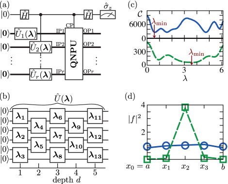
Figure 1: (a) Quantum network for summing a nonlinear function of the form $F={f^{(1)}}^{*}\prod_{j=1}^{r}(O_{j}f^{(j)})$. The ancilla qubit on the top line undergoes Hadamard gates $\hat{H}$ and controls operations of the rest of the network via the control port (CP) and is measured in the computational basis. Starting from product states $|\bm{0}\rangle$ of $n$ qubits shown as thick lines, variational states $|\psi({\bm{\lambda}})_{j}\rangle=\hat{U}_{j}({\bm{\lambda}})|\bm{0}\rangle$ representing the functions $f^{(j)}$ are created and fed to the QNPU through input ports IP. The QNPU contains problem specific quantum networks defining the linear operators $O_{j}$ and has the output ports OP. (b) Network $\hat{U}({\bm{\lambda}})$ of depth $d=5$ with $n=6$. The values ${\bm{\lambda}}=\{{\bm{\lambda}}_{1},{\bm{\lambda}}_{2},\ldots\}$ determine the form of the two-qubit gates. (c) Cost function $\mathcal{C}(\lambda)$ for the nonlinear Schrödinger equation Eq. (1) for a harmonic potential $V$, a single variational parameter $\lambda$, and $g=10^{4}$ (solid line) and $g=10$ (dashed line). The arrows indicate optimal values $\lambda=\lambda_{\rm min}$. (d) Solutions $|f(x)|^{2}$ for $\lambda=\lambda_{\rm min}$ with $N=4$ grid points and periodic boundary conditions $f(b)=f(a)$ for $g=10^{4}$ (solid line) and $g=10$ (dashed line). The circles and squares are numerically exact results. Experimental data in (c) and (d) was obtained – from a modified circuit – on IBM Q devices (see Sup for details).

We extend and adapt the concept of VQC to solving nonlinear problems efficiently on a quantum computer by virtue of two key concepts. First, we introduce a quantum nonlinear processing unit (QNPU) that efficiently calculates nonlinear functions of the form $F={f^{(1)}}^{*}\prod_{j=1}^{r}(O_{j}f^{(j)})$ for VQC. Measuring the ancilla qubit connected to the QNPU as shown in Fig. 1(a) directly yields the sum of all function values $\sum_{k}\Re\{F_{k}\}$, where $\Re\{\cdot\}$ denotes the real part. The functions $f^{(j)}$ are encoded in variational $n$-qubit states $|\psi({\bm{\lambda}})_{j}\rangle=\hat{U}_{j}({\bm{\lambda}})|\bm{0}\rangle$ created by networks of the form shown in Fig. 1(b). The same function $f^{(i)}=f^{(j)}$ may appear multiple times by choosing $\hat{U}_{i}({\bm{\lambda}})=\hat{U}_{j}({\bm{\lambda}})$. Second, we use tensor networks as a programming paradigm for QNPUs to create optimized circuits that efficiently calculate linear operators $O_{j}$ acting on functions $f^{(j)}$. In this way all quantum resources of nonlinear VQC scale polynomially with the number of qubits, which represents an exponential reduction compared with some conventional algorithms.

The variational states $|\psi({\bm{\lambda}})_{j}\rangle$ represent $N=2^{n}$ values of the functions $f^{(j)}$ which form a trial solution to the problem of interest. The cost function ${\cal C}({\bm{\lambda}})$ for nonlinear VQC is built up from outputs of different QNPUs that are then processed classically to iteratively determine the optimal set $\bm{\lambda}$. Large grid sizes that are intractable on a conventional computer require only $n\gtrsim 20$ qubits which is within reach of noisy intermediate-scale quantum (NISQ) devices. In addition, the scheme is applicable to other types of nonlinear problems that can be solved via the minimization of a cost function ${\cal C}({\bm{\lambda}})$ Griva et al. (2009).

We demonstrate the concept and performance of nonlinear VQC by emulating it classically for the canonical example of the time-independent one-dimensional nonlinear Schrödinger equation

$$\left[-\frac{1}{2}\frac{\text{d}^{2}}{\text{d}x^{2}}+V(x)+g|f(x)|^{2}\right]f(x)=Ef(x)\,,$$ (1)

where $V$ is an external potential and $g$ denotes the strength of the nonlinearity. We also implement nonlinear VQC for Eq. (1) on IBM quantum computers to establish its feasibility on current NISQ devices. Proof-of-principle results are shown in Figs. 1(c) and 1(d) demonstrating excellent agreement with numerically exact solutions. The nonlinear Schrödinger equation and its generalizations to higher dimensions describe various physical phenomena ranging from Bose-Einstein condensation to light propagation in nonlinear media Gross (1961); Pitaevskii (1961); Leggett (2001); Pitaevskii and Stringari (2003); Scott (2005); Agrawal (2013). In particular, below we consider Eq. (1) with quasi-periodic potentials $V$ that are in the focus of current cold atom experiments Viebahn et al. (2019) and that make Eq. (1) challenging to solve numerically. The methods used for this equation here are straightforwardly modified to handle other nonlinear terms and time-dependent problems as illustrated in Sup for the Burgers equation appearing in fluid dynamics.

The ground state of Eq. (1) can be found by minimizing the cost function

$$\mathcal{C}=\llangle K\rrangle_{c}+\llangle P\rrangle_{c}+\llangle I\rrangle_{c}\,,$$ (2)

where $\llangle K\rrangle_{c}$, $\llangle P\rrangle_{c}$ and $\llangle I\rrangle_{c}$ are the mean kinetic, potential and interaction energies, respectively. In Eq. (2) $\llangle\cdot\rrangle_{c}$ denotes averages with respect to a single real-valued function $f^{(1)}\equiv f$ on the interval $[a,b]$ satisfying the normalization condition $\int_{a}^{b}|f(x)|^{2}\text{d}x=1$.

In line with standard numerical approaches Press et al. (1992); Grossmann et al. (2007); Iserles (2009) we apply the finite difference method (FDM) to Eq. (1) and discretize the interval $[a,b]$ into $N$ equidistant grid points $x_{k}=a+h_{N}k$, where $h_{N}=\ell/N$ is the grid spacing, $\ell=b-a$ is the length of the interval and $k\in\{0,\ldots,N-1\}$. Each grid point is associated with a variational parameter $f_{k}$ that approximates the continuous solution $f(x_{k})$ at $x_{k}$. Furthermore, we impose periodic boundary conditions (i.e., $f_{N}=f_{0}$) and the normalization condition imposed on the continuous functions $f$ translates to

$$1=h_{N}\sum_{k=0}^{N-1}|f_{k}|^{2}=\sum_{k=0}^{N-1}|\psi_{k}|^{2}\,,$$ (3)

where $\psi_{k}=\sqrt{h_{N}}f_{k}$. Note that the condition on the set of parameters $\{\psi_{k}\}$ is independent of the grid spacing, and in the following we consider optimizing the cost function with respect to them.

All averages $\llangle\cdot\rrangle_{c}$ in Eq. (2) can be approximated by corresponding expressions of the discrete problem $\llangle\cdot\rrangle$. We find Press et al. (1992); Grossmann et al. (2007); Iserles (2009) $\llangle\cdot\rrangle_{c}=\llangle\cdot\rrangle+\mathcal{E}_{\text{grid}}$, where $\mathcal{E}_{\text{grid}}\propto 1/N^{2}$ is the error associated with the trapezoidal rule when transforming integrals into sums, and

$$\llangle K\rrangle =-\frac{1}{2}\frac{1}{h_{N}^{2}}\sum_{k=0}^{N-1}\psi_{k}^{*}\left(\psi_{k+1}-2\psi_{k}+\psi_{k-1}\right)\,,$$ (4a)

$$\llangle P\rrangle =\sum_{k=0}^{N-1}\left[\psi_{k}^{*}V(x_{k})\psi_{k}\right]\,,$$ (4b)

$$\llangle I\rrangle =\frac{1}{2}\frac{g}{h_{N}}\sum_{k=0}^{N-1}|\psi_{k}|^{4}\,.$$ (4c)

Note that $\llangle K\rrangle$ in Eq. (4a) uses a FDM representation of the second-order derivative in Eq. (1).

For evaluating the terms in Eq. (4) on a quantum computer we consider quantum registers with $n$ qubits and basis states $|\bm{q}\rangle=|q_{1}\ldots q_{n}\rangle=|q_{1}\rangle\otimes\ldots\otimes|q_{n}\rangle$, where $q_{j}\in\{0,1\}$ denotes the computational states of qubit $j$. Regarding the sequence $q_{1}\ldots q_{n}=\text{binary}(k)$ as the binary representation of the integer $k=\sum_{j=1}^{n}q_{j}2^{n-j}$, we encode all $N=2^{n}$ amplitudes $\psi_{k}$ in the normalized state

$$|\psi\rangle=\sum_{k=0}^{N-1}\psi_{k}|\text{binary}(k)\rangle\,.$$ (5)

We prepare the quantum register in a variational state $|\psi({\bm{\lambda}})\rangle$ via the quantum circuit $\hat{U}({\bm{\lambda}})$ of depth $d$ shown in Fig. 1(b). We consider depths $d\propto\text{poly}(n)$ such that the quantum ansatz requires exponentially fewer parameters $\mathcal{N}$ than standard classical schemes with $N$ parameters. Note that the number of variational parameters scales like $\mathcal{N}\propto nd$ for our quantum ansatz Sup . The power of this ansatz is rooted in the fact that it encompasses all matrix product states (MPS) Verstraete et al. (2008); Oseledets (2010, 2011); Orús (2014) with bond dimension $\chi\sim\text{poly}(n)$ Sup . Since polynomials and Fourier series Khoromskij (2011); Oseledets (2013) can be efficiently represented by MPS, the quantum ansatz simultaneously contains universal basis functions that are capable of approximating a large class of solutions to nonlinear problems efficiently. Furthermore, we show below that the quantum ansatz is capable of storing solutions with exponentially fewer resources than the classically optimized MPS ansatz. Note that the number of variational parameters scales like $\mathcal{N}\propto n\chi^{2}$ for MPS of bond dimension $\chi$ Sup .

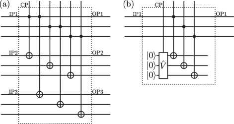
Figure 2: (a) QNPU circuit calculating the nonlinear term $|\psi|^{4}$. The networks are shown for $n=3$ and all input ports IP are fed the same variational quantum states created by $\hat{U}({\bm{\lambda}})$. IP2 is fed $\hat{U}({\bm{\lambda}})$ and IP3 is fed $\hat{U}^{*}({\bm{\lambda}})$. (b) QNPU circuit for working out the potential energy term $\tilde{V}|\psi|^{2}$.

Figure 2(a) demonstrates the basic working principle of the QNPU for the nonlinear term $\llangle I\rrangle$. The effect of the controlled NOT operations between pairs of qubits is to provide a point-wise multiplication with the ancilla thus measuring $\sum_{k}|\psi_{k}|^{4}$. In Fig. 2(b) we show the circuit for measuring $\llangle P\rrangle$. The unitary $\hat{V}\hat{=}\,O_{1}$ encodes function values of the external potential $V$. A copy of $\psi$ is effectively multiplied point-wise with the external potential by controlled NOT gates to give $\sum_{k}\tilde{V}_{k}|\psi_{k}|^{2}$. Similarly, multiplying $\psi$ with their shifted versions using adder circuits (see Sup for details) allows evaluating the kinetic energy term.

The measured expectation value of the ancilla qubit is directly related to the desired quantities as $\llangle I\rrangle=g\langle\hat{\sigma}_{z}\rangle_{\text{anc}}^{I}/2h_{N}$ for the nonlinear term, $\llangle P\rrangle=\alpha\langle\hat{\sigma}_{z}\rangle_{\text{anc}}^{P}$ for the potential energy and $\llangle K\rrangle=\left(1-\langle\hat{\sigma}_{z}\rangle_{\text{anc}}^{K}\right)/h_{N}^{2}$ for the kinetic energy Ekert et al. (2002); Alves et al. (2003). Furthermore, derivatives of the cost function, as required by some minimization algorithms Spall (1992); Griva et al. (2009); Lubasch et al. (2018), can be evaluated by combining the ideas presented here with the quantum circuits discussed in Li and Benjamin (2017); McE ; OBE ; MiN .

The unitary network $\hat{V}$ represents scaled function values $\tilde{V}_{k}$ of the external potential where $\sum_{k=0}^{N-1}|\tilde{V}_{k}|^{2}=1$, and $\alpha>0$ a scaling parameter such that $V_{k}=\alpha\tilde{V}_{k}$. Efficient quantum circuits $\hat{V}$ for measuring $\llangle P\rrangle$ can be systematically obtained by establishing tensor networks as a programming paradigm. To this end we expand the external potential in polynomials or Fourier series, $\tilde{V}(x)\approx\sum_{j}^{J}c_{j}b_{j}(x)$, where $b_{j}(x)$ are basis functions and $c_{j}$ are expansion coefficients Sup . In the case of Fourier series of order $J$, the approximate potential is represented by an MPS of bond dimension $\chi=J$ Khoromskij (2011); Oseledets (2013). Next we write the MPS in terms of $n-\lceil\log\chi\rceil$ unitaries Schön et al. (2005, 2007); Bañuls et al. (2008), where $\lceil\cdot\rceil$ is the ceiling function. Each of these unitaries acts on $2\chi$ qubits and can be decomposed in terms of elementary two-qubit gates Reck et al. (1994); Barenco et al. (1995); Shende et al. (2006); Iten et al. (2016); Sup . An upper bound for the depth of the resulting quantum circuit is $d_{>}\leq 9n[(23/48)(2\chi)^{2}+4/3]$ Shende et al. (2006). The depth thus scales polynomially with the number of qubits $n$ and with $\chi$, and many problems of interest show an even more advantageous scaling. For example, in the following we consider the potential

$$V(x)=s_{1}\sin(\kappa_{1}x)+s_{2}\sin(\kappa_{2}x)$$ (6)

and set $\kappa_{2}=2\kappa_{1}/(1+\sqrt{5})$. This potential realizes an incommensurate bichromatic lattice where the ratio $s_{1}/s_{2}$ determines the amount of disorder in the lattice Deissler et al. (2010). The trap potential $V(x)$ in Eq. (6) is exactly represented by an MPS of bond dimension $\chi=4$. The depth of the corresponding quantum circuit $d=5(n-2)+1\ll d_{>}$ is much smaller than the upper bound Sup .

Next we analyze the Monte Carlo sampling error Press et al. (1992) associated with the measurement of the ancilla qubit. We denote the absolute sampling error associated with quantity $X$ by $\mathcal{E}_{\text{MC}}^{X}$, and the corresponding relative error is Sup

$$\mathcal{\epsilon}_{\text{MC}}^{P} =\frac{\mathcal{E}_{\text{MC}}^{P}}{\llangle P\rrangle}=C_{P}\frac{1}{\sqrt{M}}\,,$$ (7a)

$$\mathcal{\epsilon}_{\text{MC}}^{K} =\frac{\mathcal{E}_{\text{MC}}^{K}}{\llangle K\rrangle}\approx C_{K}\frac{N}{N_{\text{min}}}\frac{1}{\sqrt{M}}\,,$$ (7b)

$$\mathcal{\epsilon}_{\text{MC}}^{I} =\frac{\mathcal{E}_{\text{MC}}^{I}}{\llangle I\rrangle}\approx C_{I}\frac{N}{N_{\text{min}}}\frac{1}{\sqrt{M}}\,.$$ (7c)

In this equation, we assume $N\geq N_{\text{min}}$ and $N_{\text{min}}=\ell/\ell_{\text{min}}$ is the minimal number of grid points for resolving the smallest length scale $\ell_{\text{min}}$ of the problem. The parameters $C_{X}$ in Eq. (7) are of the order of unity Sup , and all sampling errors decrease with the number of samples $M$ as $1/\sqrt{M}$. While the relative error associated with the potential term in Eq. (7a) is independent of the number of grid points, $\mathcal{\epsilon}_{\text{MC}}^{K}$ and $\mathcal{\epsilon}_{\text{MC}}^{I}$ increase linearly with $N/N_{\text{min}}$. It follows that increasing the grid size requires larger values of $M$ in order to keep the sampling error small. However, the grid error scales like $\mathcal{E}_{\text{grid}}\propto 1/N^{2}=2^{-2n}$ for $N\geq N_{\text{min}}$ Sup . We thus conclude that only moderate ratios $N/N_{\text{min}}>1$ and therefore relatively small values of $M$ are needed in order to achieve accurate solutions with small grid errors.

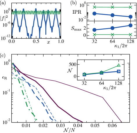
Figure 3: (a) Numerically exact solution $|f(x)|^{2}$ of Eq. (1) on a logarithmic scale, $V(x)$ in Eq. (6) with $s_{1}=2\times 10^{4}$ and $\kappa_{1}=2\pi\times 32$. The green thin line (blue normal line) is for $s_{1}/s_{2}=200$ ($s_{1}/s_{2}=2$). (b) Log-log plot of the IPR (top panel) and lin-log plot of $S_{\text{max}}$ of the exact solution $|\psi^{\text{exact}}\rangle$ (bottom panel) as a function of $\kappa_{1}$. Green crosses (blue dots) correspond to $s_{1}/s_{2}=200$ ($s_{1}/s_{2}=2$). (c) Representation error $\epsilon_{\text{R}}$ of the exact solution for the quantum ansatz (thick lines) and the MPS ansatz (thin lines) as a function of $\mathcal{N}/N$. All curves are for $s_{1}/s_{2}=2$ and correspond to $s_{1}=2\times 10^{4}$ and $\kappa_{1}=2\pi\times 32$ (green dash-dotted), $s_{1}=8\times 10^{4}$ and $\kappa_{1}=2\pi\times 64$ (blue dashed), and $s_{1}=3.2\times 10^{5}$ and $\kappa_{1}=2\pi\times 128$ (purple solid), respectively. The inset shows $\mathcal{N}$ as a function of $\kappa_{1}$ for $\epsilon_{\text{R}}=0.05$ and $s_{1}/s_{2}=2$. Blue squares (green triangles) correspond to the quantum ansatz (MPS ansatz). All curves in (a)-(c) are for $N=2^{13}=8192$ grid points and $g=50$.

The quantum ansatz in Fig. 1(b) is inspired from tensor network theory and can be regarded, for example, as the Trotter decomposition of the time $t$ evolution operator $\exp(-\mathrm{i}H(t)t/\hbar)$ of a time-dependent spin Hamiltonian $H(t)$ with arbitrary short-range interactions acting on the initial state $|\bm{0}\rangle$ Daley et al. (2004). Similarly to the coupled cluster ansatz in quantum chemistry VQC calculations Peruzzo et al. (2014), there is currently no known efficient classical ansatz for this state Trotzky et al. (2012); Schachenmayer et al. (2013). From the VQC perspective, our quantum ansatz in Fig. 1(b) is composed of generic two-qubit gates that in an experiment are accurately approximated by short sequences of gates if a sufficiently tunable or universal gate set is experimentally available Nielsen and Chuang (2010). We envisage that this quantum ansatz is more efficient than methods based on an MPS ansatz on a classical computer like the multigrid renormalization (MGR) method in Lubasch et al. (2018). This MGR method is the most efficient and accurate classical algorithm known to us for the problem considered here, for which it can already be exponentially faster than standard classical algorithms. A comparison with this powerful classical method, which is based on variational classical MPS, will allow us to validate the superior variational power of the quantum ansatz in Fig. 1(b) on a quantum computer. Note that the difficulty of solving a classical optimization problem in many variables does not go away by using the quantum ansatz, as the actual optimization is classical and there is no quantum advantage there. The quantum advantage stems solely from the faster evaluation of the cost function for our quantum ansatz in Fig. 1(b) on a quantum computer.

To provide numerical evidence for this we first obtain the numerically exact solution of Eq. (1) on the interval $[0,1]$ via the MGR algorithm Lubasch et al. (2018) and by allowing for the maximal bond dimension $\chi$ of the MPS ansatz Sup . In this case the numerically exact solution is described by $N=2^{n}$ parameters like in other conventional algorithms. The results are shown in Fig. 3 (a) for two different values of $s_{1}/s_{2}$. In the weakly disordered regime $s_{1}/s_{2}\gg 1$, $|f(x)|^{2}$ varies on the length scale set by $1/\kappa_{1}$. On the contrary, the strongly disordered regime $s_{1}/s_{2}\approx 1$ is characterized by strongly localized solutions in space. The localization of the wavefunction can be quantified using the inverse participation ratio (IPR) Kramer and MacKinnon (1993), $\text{IPR}=(N\sum_{k=0}^{N-1}|\psi_{k}|^{4})^{-1}$. We show the IPR in Fig. 3(b) as a function of $\kappa_{1}$ (top panel) and find that it stays constant for $s_{1}/s_{2}\gg 1$. On the other hand, the IPR decreases according to a power law with $\kappa_{1}$ for $s_{1}/s_{2}\approx 1$, showing that the localized character of the wavefunction increases dramatically with $\kappa_{1}$.

Next we encode the function values of the numerically exact solution in the state $|\psi^{\mathrm{exact}}\rangle$ via Eq. (5) and calculate the maximum bipartite entanglement entropy $S_{\text{max}}$ of all possible bipartitions of the $n$-qubit wave function $|\psi^{\mathrm{exact}}\rangle$. The quantity $S_{\text{max}}$ is a measure of the entanglement of $|\psi^{\mathrm{exact}}\rangle$ and is shown in the bottom panel of Fig. 3(b). The value of $S_{\text{max}}$ is small and stays constant with $\kappa_{1}$ for $s_{1}/s_{2}\gg 1$ in the weakly disordered regime. Contrary to this, for $s_{1}/s_{2}\approx 1$ in the strongly disordered regime we observe that $S_{\text{max}}\propto\log(\kappa_{1})$.

The entanglement measure $S_{\text{max}}$ provides a useful necessary criterion for efficient MPS approximations Vidal (2003). A MPS of bond dimension $\chi$ can at most contain an amount of entanglement $S_{\text{max}}[\text{MPS}]\leq\log(\chi)$ Verstraete et al. (2008); Orús (2014). For MPS to be efficient, we require that $\chi$ scales at most polynomially with $n$, i.e. $\chi=\text{poly}(n)$, so that $S_{\text{max}}[\text{MPS}]\leq\log(\text{poly}(n))$ and therefore MPS can only capture small amounts of entanglement efficiently. The small values of $S_{\text{max}}$ for $s_{1}/s_{2}\gg 1$ suggest that MPS work well in the weakly disordered regime and indeed we have confirmed numerically that this is true. Therefore, in the following we focus on the strongly disordered regime $s_{1}/s_{2}\approx 1$. In this regime MPS cannot be an efficient approximation for large values of $\kappa_{1}$: The total number of variational parameters of MPS $\mathcal{N}[\text{MPS}]$ depends quadratically on $\chi$ [35], i.e. $\mathcal{N}[\text{MPS}]\propto\chi^{2}$, and $\chi$ needs to grow polynomially with $\kappa_{1}$, i.e. $\chi\propto\text{poly}(\kappa_{1})$, to satisfy the observed entanglement scaling, such that $\mathcal{N}[\text{MPS}]\propto\text{poly}(\kappa_{1})$. Our quantum ansatz (QA) of Fig. 1(b) can capture much larger amounts of entanglement $S_{\text{max}}[\text{QA}]\lesssim d$ efficiently Schachenmayer et al. (2013) and therefore this ansatz can be an efficient approximation for large values of $\kappa_{1}$: Because the total number of variational parameters $\mathcal{N}$ depends linearly on $d$ for the quantum ansatz Sup , i.e. $\mathcal{N}[\text{QA}]\propto d$, and $d$ just needs to grow logarithmically, i.e. $d\propto\log(\kappa_{1})$, for the observed entanglement requirements, we conclude that $\mathcal{N}[\text{QA}]\propto\log(\kappa_{1})$. These entanglement considerations show that the quantum ansatz has the potential to be exponentially more efficient than MPS in the strongly disordered regime for increasing values of $\kappa_{1}$.

To quantitatively analyze and demonstrate the efficiency of the quantum ansatz in this regime, we obtain the set of parameters ${\bm{\lambda}}$ that maximize the fidelity $\mathcal{F}=|\langle\psi^{\mathrm{exact}}|\psi({\bm{\lambda}})\rangle|$ for different depths $d$ Sup . The infidelity $\epsilon_{\text{R}}=1-\mathcal{F}$ is thus a measure of the error when approximating the exact solution by this ansatz, and in the following we refer to $\epsilon_{\text{R}}$ as the representation error. As shown in Fig. 3(c), the representation error decreases exponentially as a function of $\mathcal{N}$ for all values of $\kappa_{1}$ and therefore we obtain accurate solutions for $\mathcal{N}/N\ll 1$. Even for the largest value of $\kappa_{1}=2\pi\times 128$ and $\epsilon_{\text{R}}\approx 10^{-2}$, we find $\mathcal{N}/N\approx 0.04$ so that we only require $4\%$ of the full number of parameters needed in conventional algorithms. Most importantly, the inset of Fig. 3(c) shows that, to obtain a fixed representation error of $\epsilon_{\text{R}}=0.05$, the number of parameters of our quantum ansatz needs to grow as $\mathcal{N}[\text{QA}]\propto\log(\kappa_{1})$. This numerical analysis therefore confirms our expectation, from the entanglement arguments in the previous paragraph, that the quantum ansatz efficiently approximates solutions in the strongly disordered regime even for large values of $\kappa_{1}$. This is possible because the quantum ansatz captures the required entanglement $S_{\text{max}}\propto\log(\kappa_{1})$ by means of just the small number of parameters $\mathcal{N}[\text{QA}]\propto\log(\kappa_{1})$. The entanglement capabilities of MPS imply that $\mathcal{N}[\text{MPS}]\propto\mathrm{poly}(\kappa_{1})$ has to be fulfilled. Therefore we conclude that our quantum ansatz is exponentially more efficient than MPS in the strongly disordered regime for growing values of $\kappa_{1}$. This key finding shows that nonlinear VQC can be exponentially more efficient than optimized, classical variational schemes that are based on the MPS ansatz.

We now propose a calculation that illustrates the exponential advantage of our quantum ansatz on a quantum computer particularly clearly. We consider the ground state problem of Eq. (1) with the quasi-random external potential of Eq. (6) on the interval $[0,1]$ discretized by $N=2^{n}$ equidistant grid points and use the FDM from above that leads to Eqs. (4a), (4b), and (4c). We choose $\kappa_{1}=2\pi\times 2^{n/2}$ and assume that $n=4,6,8,\ldots$ qubits store the variational quantum ansatz. The smallest wave length present in our external potential of Eq. (6) is determined by $\kappa_{1}$ and reads $2\pi/\kappa_{1}=2^{-n/2}$. The interval $[0,1]$ accomodates $1/2^{-n/2}=2^{n/2}$ of such wave lengths and our grid of $N=2^{n}$ equidistant points resolves each such wave length using $N/2^{n/2}=2^{n/2}$ grid points. Therefore the randomness of our quasi-random external potential of Eq. (6) as well as its FDM resolution grow exponentially with the number of qubits $n$. At the same time, all FDM errors (using a FDM representation of the Laplace operator, the trapezoidal rule for integration, and so on) decrease polynomially with the grid spacing $1/N=2^{-n}$ and thus exponentially with $n$. Therefore, with growing values of $n$, our FDM representation of Eq. (1) converges exponentially fast to the continuous problem and the accuracy of randomness in Eq. (6) grows exponentially. Our proposal is to solve this problem for the strongly disordered regime $s_{1}/s_{2}\approx 1$ in Eq. (6), i.e. compute the corresponding ground states, using an increasing number $n=4,6,8,\ldots$. Based on the numerical analysis of Fig. 3, we conjecture that MPS require resources $\mathcal{N}[\text{MPS}]\propto\text{poly}(\kappa_{1})=\text{poly}(2\pi\times 2^{n/2})=\text{exp}(n)$ growing exponentially with $n$, whereas the quantum ansatz of Fig. 1(b) just needs resources $\mathcal{N}[\text{QA}]\propto\log(\kappa_{1})=\log(2\pi\times 2^{n/2})=\text{poly}(n)$ increasing polynomially with $n$. This calculation can be used to demonstrate quantum supremacy as, by successively increasing $n$, the limit of what is computationally possible on a classical computer (using MPS or exact classical methods) is reached quickly and our quantum ansatz on a quantum computer remains efficient far beyond this classical limit.

The quantum hardware requirements for this quantum supremacy calculation go beyond the current capabilities of available NISQ devices Cross et al. (2019). Nevertheless the superior performance of our quantum ansatz is relevant for current NISQ devices as only the most efficient variational states can succeed in the presence of the current experimental errors. We test the feasibility of nonlinear VQC on NISQ devices by calculating the ground state of Eq. (1) for a simple harmonic potential and a single variational parameter on an IBM Q device ibm utilizing further network optimizations (see Sup for details). The experimental implementation of the nonlinear VQC algorithm was able to identify the optimal variational parameter with an error of less than $10\%$ leading to excellent agreement of the ground state solutions with exact numerical solutions [c.f. Figs. 1(c)(d)].

The methods presented here are readily modified to two-and three-dimensional problems with an overhead scaling linearly in the number of dimensions, and can be applied to a broad range of nonlinear terms and differential operators. An exciting prospect for future work will be to utilize intermediate-scale quantum computers for solving non-linear problems on grid sizes beyond the scope of conventional computers.