On jump relations of anisotropic elliptic interface problems

Abstract

Almost all materials are anisotropic. In this paper, interface relations of anisotropic elliptic partial differential equations involving discontinuities across interfaces are derived in two and three dimensions. Compared with isotropic cases, the invariance of partial differential equations and the jump conditions under orthogonal coordinates transformation is not valid anymore. A systematic approach to derive the interface relations is established in this paper for anisotropic elliptic interface problems, which can be important for deriving high order accurate numerical methods.

keywords: anisotropic elliptic interface problems, jump conditions/relations, local coordinates.

AMS Subject Classification 2000 .

1 Introduction

Consider an anisotropic elliptic interface problem below,

$$\begin{array}[]{rcl}&&\displaystyle-\nabla\cdot\left(\mathbf{A}(\mathbf{x})\nabla u(\mathbf{x})\right)+\sigma(\mathbf{x})u(\mathbf{x})=f(\mathbf{x}),\qquad\mathbf{x}\in\Omega\setminus\Gamma,\quad\Omega=\Omega^{+}\cup\Omega^{-},\end{array}$$ (1)

where $\mathbf{A}(\mathbf{x})\in C(\Omega\setminus\Gamma)$ is a symmetric positive definite matrix whose eigenvalues satisfy, $\lambda_{i}(\mathbf{x})\geq\lambda_{0}>0$, for all $\mathbf{x}\in\Omega$; and $\sigma(\mathbf{x})\geq 0$; the source term $f(\mathbf{x})\in C(\Omega\setminus\Gamma)$.

$$[u]=w,\qquad[{\bf A}\nabla u\cdot\mathbf{n}]=v,$$ (2)

where $\Gamma\in C^{2}$ is a smooth interface with the solution domain, and the notation $[\;]$ is a jump of a quantity across the interface. The above jump conditions are often referred as internal boundary conditions that make the problem well-posed.

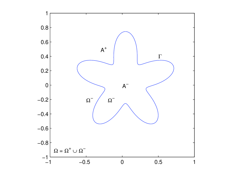
Figure 1: (a): A diagram of a domain $\Omega$ with an interface $\Gamma$. (b): A local coordinates.

There are many discussions in the literature about anisotropic interface problems including physics and modeling [2, 8, 10], analysis [11, 6, 12], and numerical methods [4, 1, 5].

For theoretical and numerical purposes, we want to know the interface relations of the partial derivatives of the solution across the interface. When ${\bf A}=\beta{\bf I}$, that is, a scalar case, the interface relations have been derived using the invariance of the PDE and the jump conditions. The derived interface relations have then been applied in derive accurate finite difference methods such as the IIM [7, 3, 9].

2 The interface relations for anisotropic interface problems in 2D

In 2D, the interface $\Gamma$ is a curve within the solution domain. We cannot assume invariances of the PDE, the flux jump conditions, and their surface derivatives under different coordinates systems. In this paper, we propose a way to parameterize the interface locally using a level set function so that we can derive the interface relations in a systematically way as described below.

2.1 The local coordinate system and representation of the interface in 2D

Let $(X^{*},Y^{*})$ be a fixed point on the interface $\Gamma$, and the normal direction at $(X^{*},Y^{*})$ be $(\cos\theta^{*},\sin\theta^{*})$, where $\theta^{*}$ is the angle of the normal direction and the $x$-axis, see Figure 1 for an illustration. The local coordinates in the neighborhood of $(X^{*},Y^{*})$ is defined as

$$\begin{array}[]{rcl}\left\{\begin{array}[]{l}\xi=\displaystyle(x-X^{*})\,\mbox{cos}\,\theta^{*}+(y-Y^{*})\,\mbox{sin}\,\theta^{*},\\ \vskip 5.0pt\cr\eta=-(x-X^{*})\,\mbox{sin}\,\theta^{*}+(y-Y^{*})\,\mbox{cos}\,\theta^{*}.\end{array}\right.\end{array}$$ (3)

In a neighborhood of $(X^{*},Y^{*})$, the interface can be written as

$$\xi=\chi(\eta),\quad\mbox{with}\quad\chi(0)=0,\quad\chi^{\prime}(0)=0,$$ (4)

and can be further parameterized as

$$\begin{array}[]{rcl}\left\{\begin{array}[]{l}X(s)=\displaystyle X^{*}+\chi(s)\,\mbox{cos}\,\theta^{*}-s\,\mbox{sin}\,\theta^{*},\\ \vskip 5.0pt\cr Y(s)=Y^{*}+\chi(s)\,\mbox{sin}\,\theta^{*}+s\,\mbox{cos}\,\theta^{*}.\end{array}\right.\end{array}$$ (5)

We have $(X(0),Y(0))=(X^{*},Y^{*})$, here $s$ can be regarded as arc-length parameter starting from $(X^{*},Y^{*})$. The tangent vector then is

$$\begin{array}[]{rcl}\mbox{\boldmath$\tau$}(s)&=&\displaystyle\left[\frac{X^{\prime}}{\sqrt{(X^{\prime})^{2}+(Y^{\prime})^{2}}},\;\frac{Y^{\prime}}{\sqrt{(X^{\prime})^{2}+(Y^{\prime})^{2}}}\right]\\ \vskip 5.0pt\cr&=&\displaystyle\left[\frac{\chi^{\prime}\,\cos\theta^{*}-\sin\theta^{*}}{\sqrt{1+(\chi^{\prime})^{2}}},\;\frac{\chi^{\prime}\,\sin\theta^{*}+\cos\theta^{*}}{\sqrt{1+(\chi^{\prime})^{2}}}\right],\end{array}$$ (6)

with $\mbox{\boldmath$\tau$}(0)=[-\sin\theta^{*},\;\cos\theta^{*}]$, and the normal direction is

$$\begin{array}[]{rcl}\mathbf{n}=\displaystyle\left[\frac{\chi^{\prime}\,\sin\theta^{*}+\cos\theta^{*}}{\sqrt{1+(\chi^{\prime})^{2}}},\;\frac{-\chi^{\prime}\,\cos\theta^{*}+\sin\theta^{*}}{\sqrt{1+(\chi^{\prime})^{2}}}\right].\end{array}$$ (7)

For simplicity, we still use the same notations for the solution $u$, ${\bf A}$, $[u]=w(s)$, and $[{\bf A}\nabla u\cdot{\bf n}]=v(s)$ in the local coordinate system. In the neighborhood of $(X^{*},Y^{*})$, using the idea of the level set method, we can extend the quantities on the interface along the normal line using $\varphi(\xi,s)=\xi-\chi(s)$. Thus the tangential and normal derivatives and other interface quantities are also defined in the neighborhood as the normal extension of their value from the interface along the normal line. Note that in the local coordinates, the PDE can be written as

$$a_{11}u_{\xi\xi}+2a_{12}u_{\xi\eta}+a_{22}u_{\eta\eta}-\sigma u=f,$$ (8)

where $a_{ij}$ are defined below

$$\begin{array}[]{rcl}a_{11}&=&\displaystyle A_{11}\cos^{2}\theta^{*}+A_{22}\sin^{2}\theta^{*}+2A_{12}\cos\theta^{*}\sin\theta^{*},\\ \vskip 5.0pt\cr a_{22}&=&\displaystyle A_{11}\sin^{2}\theta^{*}+A_{22}\cos^{2}\theta^{*}-2A_{12}\cos\theta^{*}\sin\theta^{*},\\ \vskip 5.0pt\cr a_{12}&=&\displaystyle\left(A_{22}-A_{11}\right)\cos\theta^{*}\sin\theta^{*}+A_{12}\left(\cos^{2}\theta^{*}-\sin^{2}\theta^{*}\right).\end{array}$$ (9)

Under the framework above, we are ready to prove the main theorem in 2D.

Theorem 1

If ${\bf A}$ is a piecewise constant matrix, $u(x,y)\in C^{2}(\Omega^{\pm})$, $f(x,y)\in C(\Omega^{\pm})$, $\Gamma\in C^{2}$, $w\in C^{2}$, $v\in C^{1}$, then the following interface relations hold.

$$\begin{array}[]{rcl}&&u^{+}=u^{-}+w\\ \vskip 5.0pt\cr&&\displaystyle u_{\xi}^{+}=\frac{a^{-}_{11}}{a^{+}_{11}}u_{\xi}^{-}-\frac{[a_{12}]}{a^{+}_{11}}u_{\eta}^{-}+\frac{1}{a^{+}_{11}}v-\frac{a^{+}_{12}}{a^{+}_{11}}w^{\prime}\\ \vskip 5.0pt\cr&&\displaystyle u_{\eta}^{+}=u_{\eta}^{-}+w^{\prime}\\ \vskip 5.0pt\cr&&\displaystyle u_{\eta\eta}^{+}=\chi^{\prime\prime}\frac{[a_{11}]}{a^{+}_{11}}u_{\xi}^{-}+\chi^{\prime\prime}\frac{[a_{12}]}{a^{+}_{11}}u_{\eta}^{-}+u_{\eta\eta}^{-}-\frac{\chi^{\prime\prime}}{a^{+}_{11}}v+\chi^{\prime\prime}\frac{a^{+}_{12}}{a^{+}_{11}}w^{\prime}+w^{\prime\prime}\\ \vskip 5.0pt\cr&&\displaystyle u_{\xi\eta}^{+}=\chi^{\prime\prime}\frac{a^{+}_{11}[a_{12}]-2a^{+}_{12}[a_{11}]}{(a^{+}_{11})^{2}}u_{\xi}^{-}+\chi^{\prime\prime}\frac{a^{+}_{11}[a_{22}]-2a^{+}_{12}[a_{12}]}{(a^{+}_{11})^{2}}u_{\eta}^{-}+\frac{a^{-}_{11}}{a^{+}_{11}}u_{\xi\eta}^{-}\\ \vskip 5.0pt\cr&&\displaystyle\hbox{}\quad-\frac{[a_{12}]}{a^{+}_{11}}u_{\eta\eta}^{-}+\chi^{\prime\prime}\frac{2a^{+}_{12}}{(a^{+}_{11})^{2}}v+\frac{1}{a^{+}_{11}}v^{\prime}+\chi^{\prime\prime}\frac{(a^{+}_{11}a^{+}_{22}-2(a^{+}_{12})^{2})}{(A^{+}_{11})^{2}}w^{\prime}-\frac{a^{+}_{12}}{a^{+}_{11}}w^{\prime\prime}\\ \vskip 5.0pt\cr&&\displaystyle u_{\xi\xi}^{+}=-S_{1}\chi^{\prime\prime}u_{\xi}^{-}-S_{2}\chi^{\prime\prime}u_{\eta}^{-}+\frac{a_{11}^{-}}{a_{11}^{+}}u_{\xi\xi}^{-}+\frac{2a_{12}^{+}[a_{12}]-a_{11}^{+}[a_{22}]}{(a_{11}^{+})^{2}}u_{\xi\eta}^{-}\\ \vskip 5.0pt\cr&&\displaystyle\hbox{}\qquad\qquad+\frac{2(a_{12}^{+}[a_{11}]-a_{11}^{+}[a_{12}])}{(a_{11}^{+})^{2}}u_{\eta\eta}^{-}+\frac{[f]}{a_{11}^{+}}+\frac{[\sigma]}{a^{+}_{11}}u^{-}+S_{3},\end{array}$$ (10)

where $S_{1}$, $S_{2}$, and $S_{3}$ are given below,

$$\begin{array}[]{rcl}S_{1}&=&\displaystyle\frac{2a_{11}^{+}a_{12}^{+}[a_{12}]-4(a_{12}^{+})^{2}[a_{11}]+a_{11}^{+}a_{22}^{+}[a_{11}]}{(a_{11}^{+})^{3}}\\ \vskip 5.0pt\cr S_{2}&=&\displaystyle-\chi^{\prime\prime}\frac{2a_{11}^{+}a_{12}^{+}[a_{22}]-4(a_{12}^{+})^{2}[a_{12}]+a_{11}^{+}a_{22}^{+}[a_{12}]}{(a_{11}^{+})^{3}}\\ \vskip 5.0pt\cr S_{3}&=&\displaystyle-\chi^{\prime\prime}\frac{4(a_{12}^{+})^{2}-a_{11}^{+}a_{22}^{+}}{(a_{11}^{+})^{3}}v-\frac{2a_{12}^{+}}{(a_{11}^{+})^{2}}v^{\prime}\\ \vskip 5.0pt\cr&&\hbox{}\quad\displaystyle+\frac{\sigma^{+}w}{a^{+}_{11}}-\chi^{\prime\prime}\frac{a_{11}^{+}a_{12}^{+}a_{22}^{+}-4(a_{12}^{+})^{3}}{(a_{11}^{+})^{3}}w^{\prime}+\frac{2(a_{12}^{+})^{2}-a_{11}^{+}a_{12}^{+}}{(a_{11}^{+})^{2}}w^{\prime\prime}.\end{array}$$ (11)

Note that $S_{3}$ depends on the jump conditions $w$ and $v$, their (surface) derivatives, coefficient matrix ${\bf A}$, and the curvature of $\Gamma$.

Proof: Differentiating $[u]=w$ with respect to $s$ once we get

$$[u_{\xi}]\;\chi^{\prime}+[u_{\eta}]=w^{\prime}(s).$$ (12)

Differentiating the identity above with respect to $s$ we get

$$[u_{\xi\xi}]\chi^{\prime 2}+2[u_{\xi\eta}]\chi^{\prime}+[u_{\xi}]\chi^{\prime\prime}+[u_{\eta\eta}]=w^{\prime\prime}(s).$$ (13)

Setting $s=0$ in the above two identities and using $\chi^{\prime}(0)=0$, we obtain the third and the fourth identities in the theorem.

From $u_{x}=u_{\xi}\cos\theta^{*}-u_{\eta}\sin\theta^{*}$, $u_{y}=u_{\xi}\sin\theta^{*}+u_{\eta}\cos\theta^{*}$ and $\mathbf{n(s)}$ defined above, and the relation between $A_{ij}$ and $a_{ij}$, and with some manipulations, we can rewrite $\big{[}\mathbf{A}\nabla u\cdot\mathbf{n}\big{]}$ as,

$$\big{[}\mathbf{A}\nabla u\cdot\mathbf{n}\big{]}=\left[\left(\begin{array}[]{cc}A_{11}&A_{12}\\ A_{12}&A_{22}\\ \end{array}\right)\left(\begin{array}[]{c}u_{x}\\ u_{y}\\ \end{array}\right)\cdot\left(\begin{array}[]{c}n_{x}\\ n_{y}\\ \end{array}\right)\right]$$

$$=\bigg{[}\left(\begin{array}[]{c}A_{11}(u_{\xi}\cos\theta^{*}-u_{\eta}\sin\theta^{*})+A_{12}(u_{\xi}\sin\theta^{*}+u_{\eta}\cos\theta^{*})\\ A_{12}(u_{\xi}\cos\theta^{*}-u_{\eta}\sin\theta^{*})+A_{22}(u_{\xi}\sin\theta^{*}+u_{\eta}\cos\theta^{*})\\ \end{array}\right)^{T}\cdot\mathbf{n}\bigg{]}$$

$$=\frac{1}{\sqrt{1+(\chi^{\prime})^{2}}}\left[\frac{\hbox{}}{\hbox{}}\left(a_{11}-\chi^{\prime}a_{12}\right)u_{\xi}]+\left[(a_{12}-\chi^{\prime}a_{22}\right)u_{\eta}\right].$$

Therefore, the flux jump condition can be written as

$$\left[\frac{\hbox{}}{\hbox{}}\left(a_{11}-\chi^{\prime}a_{12}\right)u_{\xi}\right]+\left[\frac{\hbox{}}{\hbox{}}\left(a_{12}-\chi^{\prime}a_{22}\right)u_{\eta}\right]=\sqrt{1+(\chi^{\prime})^{2}}\,v(s).$$ (14)

We get the second identity by setting $s=0$.

To get the fifth identity, we differentiate the flux jump condition above with respect to $s$. The left hand side then is

$$LHS = \left[\frac{\hbox{}}{\hbox{}}\left(a_{11}-\chi^{\prime}a_{12}\right)\left(u_{\xi\xi}\chi^{\prime}+u_{\xi\eta}\right)\right]+\left[\frac{\hbox{}}{\hbox{}}-\chi^{\prime\prime}a_{12}u_{\xi}\right]$$

$$\hbox{}+\left[\frac{\hbox{}}{\hbox{}}\left(a_{12}-\chi^{\prime}a_{22}\right)\left(u_{\eta\xi}\chi^{\prime}+u_{\eta\eta}\right)\right]+\left[\frac{\hbox{}}{\hbox{}}-\chi^{\prime\prime}a_{22}u_{\eta}\right].$$

The right hand side is

$$RHS=\sqrt{1+(\chi^{\prime})^{2}}\,v^{\prime}(s)+\frac{\chi^{\prime}\chi^{\prime\prime}}{\sqrt{1+(\chi^{\prime})^{2}}}\,v(s).$$

By plugging $s=0$ to the left and right hand sides and using $\chi^{\prime}(0)=0$, we get the fifth identity.

The last identity is obtained from the PDE using

$$[a_{11}u_{\xi\xi}]+2[a_{12}u_{\xi\eta}]+[a_{22}u_{\eta\eta}]-[\sigma u]=[f].$$ (15)

Remark 1

For variable coefficients ${\bf A({\bf x}})$, $\sigma({\bf x})$, and $f({\bf x})$, the derivation process is similar but the expressions are long and more complicated. The PDE in the local coordinates now is

$$a_{11}u_{\xi\xi}+2a_{12}u_{\xi\eta}+a_{22}u_{\eta\eta}+c_{1}u_{\xi}+c_{2}u_{\eta}-\sigma u=f,$$ (16)

where

$$c_{1}=\frac{\partial a_{11}}{\partial\xi}+\frac{\partial a_{12}}{\partial\eta},\qquad c_{2}=\frac{\partial a_{12}}{\partial\xi}+\frac{\partial a_{22}}{\partial\eta}$$ (17)

The first four identities are the same and the last two are the following:

$$\begin{array}[]{rcl}u^{+}_{\xi\eta}&=&\displaystyle\frac{c^{-}_{3}[a_{11}]-a_{11}^{-}[c_{3}]-\chi^{\prime\prime}a^{+}_{12}[a_{11}]}{(a_{11}^{+})^{2}}u^{-}_{\xi}+\frac{c^{+}_{3}[a_{12}]-a_{11}^{+}[c_{4}]-\chi^{\prime\prime}a^{+}_{12}[a_{12}]}{(a_{11}^{+})^{2}}u^{-}_{\eta}-\frac{[a_{12}]}{a_{11}^{+}}u^{-}_{\eta\eta}\\ \vskip 5.0pt\cr&&\displaystyle\hbox{}+\frac{a_{11}^{-}}{a_{11}^{+}}u^{-}_{\xi\eta}+\frac{c^{+}_{3}a^{+}_{12}-a_{11}^{+}c^{+}_{4}-\chi^{\prime\prime}(a^{+}_{12})^{2}}{(a_{11}^{+})^{2}}w^{\prime}-\frac{a_{12}^{+}}{a_{11}^{+}}w^{\prime\prime}+\frac{\chi^{\prime\prime}a^{+}_{12}-c^{+}_{3}}{(a_{11}^{+})^{2}}v+\frac{v^{\prime}}{a_{11}^{+}},\end{array}$$ (18)

$$\begin{array}[]{rcl}u^{+}_{\xi\xi}&=&\displaystyle\frac{(a_{11}^{+})^{2}c^{-}_{1}-a_{11}^{+}a_{11}^{-}c^{+}_{1}-2a^{+}_{12}(c^{-}_{3}[a_{11}]-a_{11}^{-}[c_{3}]-\chi^{\prime\prime}a^{+}_{12}[a_{11}])-\chi^{\prime\prime}a^{+}_{11}a^{+}_{22}[a_{11}]}{(a_{11}^{+})^{3}}u^{-}_{\xi}\\ \vskip 5.0pt\cr&&\displaystyle\hbox{}+\frac{a_{11}^{+}c^{+}_{1}[a_{12}]-(a_{11}^{+})^{2}[c_{2}]-2a^{+}_{12}(c^{+}_{3}[a_{12}]-a_{11}^{+}[c_{4}]-\chi^{\prime\prime}a^{+}_{12}[a_{12}])-\chi^{\prime\prime}a^{+}_{11}a^{+}_{22}[a_{12}]}{(a_{11}^{+})^{3}}u^{-}_{\eta}\\ \vskip 5.0pt\cr&&\displaystyle\hbox{}+\frac{a_{11}^{-}}{a_{11}^{+}}u^{-}_{\xi\xi}+\frac{2a^{+}_{12}[a_{12}]-a^{+}_{11}[a_{22}]}{(a_{11}^{+})^{2}}u^{-}_{\eta\eta}+\frac{2(a^{+}_{12}[a_{11}]-a^{+}_{11}[a_{12}])}{(a_{11}^{+})^{2}}u^{-}_{\xi\eta}\\ \vskip 5.0pt\cr&&\displaystyle\hbox{}+\frac{a_{11}^{+}a^{+}_{12}c^{+}_{1}-(a_{11}^{+})^{2}c^{+}_{2}-2a^{+}_{12}(c^{+}_{3}a^{+}_{12}-a_{11}^{+}c^{+}_{4}-\chi^{\prime\prime}(a^{+}_{12})^{2})-\chi^{\prime\prime}a_{11}^{+}a_{12}^{+}a_{22}^{+}}{(a_{11}^{+})^{3}}w^{\prime}\\ \vskip 5.0pt\cr&&\displaystyle\hbox{}+\frac{2(a_{12}^{+})^{2}-a_{11}^{+}a_{22}^{+}}{a_{11}^{+}}w^{\prime\prime}+\frac{\chi^{\prime\prime}a^{+}_{11}a^{+}_{22}-a^{+}_{11}c^{+}_{1}-2a^{+}_{12}(\chi^{\prime\prime}a^{+}_{12}-c^{+}_{3})}{(a_{11}^{+})^{3}}v-\frac{2a^{+}_{12}}{(a_{11}^{+})^{2}}v^{\prime}\\ \vskip 5.0pt\cr&&\displaystyle\hbox{}+\frac{\sigma^{+}[u]+[\sigma]u^{-}}{a_{11}^{+}}+\frac{[f]}{a_{11}^{+}},\end{array}$$ (19)

where $c_{k}$, $k=1,2,3,4$ are given below where

$$c_{1}=\frac{\partial a_{11}}{\partial\xi}+\frac{\partial a_{12}}{\partial\eta},\quad c_{2}=\frac{\partial a_{12}}{\partial\xi}+\frac{\partial a_{22}}{\partial\eta},\quad c_{3}=\frac{\partial a_{11}}{\partial\eta}-\chi^{\prime\prime}a_{12},\quad c_{4}=\frac{\partial a_{12}}{\partial\eta}-\chi^{\prime\prime}a_{22}.$$ (20)