Hydrodynamics of two-dimensional compressible fluid with broken parity:
variational principle and free surface dynamics in the absence of dissipation

Abstract

We consider an isotropic compressible non-dissipative fluid with broken parity subject to free surface boundary conditions in two spatial dimensions. The hydrodynamic equations describing the bulk dynamics of the fluid as well as the free surface boundary conditions depend explicitly on the parity breaking non-dissipative odd viscosity term. We construct a variational principle in the form of an effective action which gives both bulk hydrodynamic equations and free surface boundary conditions. The free surface boundary conditions require an additional boundary term in the action which resembles a $1+1D$ chiral boson field coupled to the background geometry. We solve the linearized hydrodynamic equations for the deep water case and derive the dispersion of chiral surface waves. We show that in the long wavelength limit the flow profile exhibits an oscillating vortical boundary layer near the free surface. The thickness of the layer is controlled by the length scale given by the ratio of odd viscosity to the sound velocity $\delta\sim\nu_{o}/c_{s}$. In the incompressible limit, $c_{s}\to\infty$ the vortical boundary layer becomes singular with the vorticity within the layer diverging as $\omega\sim c_{s}$. The boundary layer is formed by odd viscosity coupling the divergence of velocity $\bm{\nabla}\cdot\bm{v}$ to vorticity $\bm{\nabla}\times\bm{v}$. It results in non-trivial chiral free surface dynamics even in the absence of external forces. The structure of the odd viscosity induced boundary layer is very different from the conventional free surface boundary layer associated with dissipative shear viscosity.

Introduction. In a seminal work, Avron  avron1998odd noticed that in two spatial dimensions the viscosity tensor allows for a parity breaking term, dubbed odd viscosity, without breaking the fluid isotropy. The recent interest in this parity violating stress-shear response was triggered by Ref. avron1995viscosity , which shows that the odd viscosity coefficient is quantized for quantum Hall systems, where it is related to the adiabatic curvature on the space of flat background metrics on a torus. Several theoretical works subsequently studied odd viscosity, also known as Hall viscosity, as a new quantized observable of quantum Hall fluids tokatly2006magnetoelasticity ; tokatly2007new ; tokatly2009erratum ; read2009non ; haldane2011geometrical ; haldane2011self ; hoyos2012hall ; bradlyn2012kubo ; yang2012band ; abanov2013effective ; hughes2013torsional ; hoyos2014hall ; laskin2015collective ; can2014fractional ; can2015geometry ; klevtsov2015geometric ; klevtsov2015quantum ; gromov2014density ; gromov2015framing ; gromov2016boundary ; scaffidi2017hydrodynamic ; andrey2017transport ; alekseev2016negative ; pellegrino2017nonlocal . Other classes of fluid systems where ‘odd viscous’ effects might be important include polyatomic gases korving1966transverse ; knaap1967heat ; korving1967influence ; hulsman1970transverse , chiral active matter banerjee2017odd ; souslov2019topological ; soni2018free , vortex dynamics in two dimensions wiegmann2014anomalous ; yu2017emergent ; bogatskiy2018edge ; bogatskiy2019vortex , chiral superfluids/superconductors read2009non ; hoyos2014effective and any fluid dynamics with parity breaking intrinsic angular momentum of constituent particles. Experimentally, odd viscosity can be indirectly measured through corrections to the charge transport (see, e.g., Ref. berdyugin2019measuring ) or more directly in chiral active fluids by observing the dynamics of the boundary of a fluid with odd viscosity soni2018free . It was also shown that if the fluid is almost incompressible, the odd viscosity $\nu_{o}$ effects are most visible at the dynamical boundary subject to no-stress (free surface) boundary conditions ganeshan2017odd ; abanov2018odd .

A classic example of no-stress dynamical boundary conditions is that of surface gravity waves. For perfect fluids without any viscosities, the irrotational surface dynamics was solved by Stokes in 1847 george1847stokes , when he derived the famous surface gravity wave dispersion relation $\Omega=\pm\sqrt{g|k|}$ .

The presence of infinitesimal shear viscosity requires tangent stress induced vorticity near the moving boundary thereby violating irrotationality. This effect can be captured within linearized hydrodynamics, where a small but finite shear viscosity creates a thin vortical boundary layer of thickness $\delta\sim\sqrt{\nu_{e}/\Omega}$ near the surface of the fluid lamb1932hydrodynamics . The fluid outside this layer remains irrotational to an excellent approximation . The presence of odd viscosity in addition to shear viscosity significantly alters this boundary layer structure as shown by some of us in Ref. abanov2018odd . While the thickness of the boundary layer is still controlled by $\delta\sim\sqrt{\nu_{e}/\Omega}$, in the limit $\nu_{e}\rightarrow 0$ (with fixed $\nu_{o}$), the vorticity $\omega=\bm{\nabla}\times\bm{v}$ within the layer diverges as $\omega\sim\frac{1}{\sqrt{\nu_{e}}}$ abanov2018odd . Therefore, the limit $\nu_{e}\to 0$ is singular and can be thought of as the formation of a discontinuity in the velocity component tangential to the fluid boundary. This discontinuity makes it difficult to access free surface results for fluids with exactly zero shear viscosity $\nu_{e}=0$ (to be contrasted with the limit $\nu_{e}\to 0$ abanov2018odd ).

Strictly non-dissipative fluids with $\nu_{e}=0$ are of considerable interest, with notable examples being quantum Hall fluids and superfluids. Therefore, in this work we consider a strictly non-dissipative fluid with odd viscosity and free boundary. The dissipationless nature of such a fluid allows for a variational principle description, which produces both bulk hydrodynamic equations and appropriate free surface boundary conditions.

The solution to the linearized hydrodynamic equations with free surface shows that a finite compressibility is needed to satisfy the no-stress boundary conditions at the free surface without appealing to weak solutions with discontinuities. The incompressible limit is therefore subtle and characterized by the formation of a singular boundary layer whose thickness is controlled by a new length scale $\delta\sim\nu_{o}/c_{s}$ (ratio of odd viscosity to sound velocity) with diverging vorticity ($\omega\sim c_{s}$).

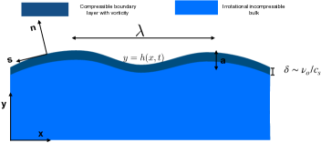
Figure 1: Schematic of the free surface dynamics of an infinitely deep two-dimensional “ocean”.

Hydrodynamics of compressible fluid with odd viscosity. Hydrodynamic equations consist of the conservation equations for local mass and momentum footnote-energy , assuming all other relevant quantities are equilibrated. The momentum conservation and continuity equation can be written in terms of the mass density of the fluid $\rho$ and its velocity $v_{i}$ as,

$$\partial_{t}\rho+\partial_{i}(\rho v_{i})=0\,,\;\partial_{t}(\rho v_{i})+\partial_{j}(\rho v_{i}v_{j}-T_{ij})=\rho F_{i}\,.$$ (1)

Here we assumed that the fluid is charged so that the external force in the presence of electromagnetic fields is given by $F_{i}=-e(B\epsilon_{ij}v_{j}+E_{i})/m$ with $\epsilon_{ij}$ being the Levi-Civita tensor. Additionally, we assume that the ratio between charge and mass density is constant and proportional to $-e/m$. In the following we set $e/m=1$. For simplicity, we neglect thermal effects in this paper and do not consider local energy conservation footnote-energy , since it follows directly from the equations for momentum and mass conservation.

For a fluid with odd viscosity, the stress tensor $T_{ij}$ in Eq. (1) is given by avron1998odd

$$T_{ij}=-p\,\delta_{ij}+\nu_{o}\rho(\partial_{i}^{*}v_{j}+\partial_{i}v_{j}^{*})\,,$$ (2)

where $\nu_{o}$ is called kinematic odd viscosity. Here and in the following, we use the star operation defined by $a_{i}^{*}\equiv\epsilon_{ij}a_{j}$. The pressure $p$ in Eq. (2) must be understood as a function of the density $p(\rho)$ . Both the parameter $\nu_{o}$ and the equation of state $p(\rho)$ are supposed to be derived from an underlying microscopic model and are assumed to be known in the rest of the Letter. Formally, the incompressible limit can be achieved by taking the limit of infinite sound velocity $c_{s}\to\infty$, where $c_{s}=\sqrt{dp/d\rho}$.

Eqs. (1) and (2) are often referred to as the first-order hydrodynamics, emphasizing the fact that the gradient expansion of the stress tensor (2) is stopped at the first order in spatial derivatives of velocity. It is well known that in the hydrodynamics with gradient terms the velocity of the fluid is not uniquely defined . One could fix the definition of velocity by saying that the mass density current entering the continuity equation in (1) is given by $\rho v_{i}$. Alternatively, one could insist on $\rho v_{i}$ being the momentum density entering the second equation in (1). In the following, we assume that for the fluid under consideration the momentum density and the mass current density are identical and given by $\rho v_{i}$. This may not be true in a particular microscopically realized fluid (see, e.g., moroz2019bosonic ) and the results presented in this letter will change. However, it is straightforward to generalize our calculations to such cases.

For a fluid domain with boundaries, we must supply boundary conditions to the bulk equations of motion in (1). The fluid free surface is a dynamical interface $\Gamma$ between two fluids where we impose one kinematic and two dynamical boundary conditions

$$(\partial_{t}\Gamma)_{n}=v_{n}\Big{|}_{\Gamma}\,,\qquad n_{i}T_{ij}\Big{|}_{\Gamma}=0\,.$$ (3)

Here $n_{i}\equiv(n_{x},n_{y})$ are the components of the unit vector outward normal to the free surface $\Gamma$ (see Figure 1). The equation on the left is the kinematic boundary condition which states that the velocity of the fluid normal to the boundary is equal to the speed of the boundary. The pair of equations on the right states that there are no normal and tangent forces acting on an element of the fluid surface. It is important to realize that both conditions depend on how we parametrize momentum density and mass current in terms of the velocity field. The normal velocity $v_{n}$ entering the first condition arises from the mass current density, while the dynamic boundary conditions are given in terms of the stress tensor components $T_{ij}$. The velocity dependence in Eq. (2) comes from the identification of the fluid momentum density with $\rho v_{i}$.

Variational principle. The fluid dynamics described in Eqs. (1-3) is non-dissipative (see footnote-energy ). The absence of dissipation allows us to capture the full bulk and boundary dynamics in a variational principle. For that we parametrize the flow velocity in terms of three scalar fields $(\theta,\alpha,\gamma)$, known as Clebsch potentials

$$v_{i}=u_{i}-\nu_{o}\partial_{i}^{*}\ln\rho\,,\quad u_{\mu}\equiv\partial_{\mu}\theta+A_{\mu}+\alpha\partial_{\mu}\gamma\,,$$ (4)

where $i=1,2$ and $\mu=0,1,2$. For an introduction to Clebsch parametrization we refer to Ref. 1997-ZakharovKuznetsov and references therein.

Let the fluid domain $\mathcal{M}$ be given by $y\leq h(t,x)$ and let $\varepsilon(\rho)$ be the internal energy density of the fluid. Using the definition (4), the hydrodynamic action can be written as

$$S=S_{\mathcal{M}}+\,S_{\Gamma}\,,$$ (5)

$$S_{\mathcal{M}}=-\iint dt\,dx\int\limits_{-\infty}^{h(t,x)}dy\Big{[}\rho\left(u_{0}+\tfrac{1}{2}v_{i}^{2}\right)+\varepsilon(\rho)\Big{]}\,,$$ (6)

$$S_{\Gamma}=\nu_{o}\iint dt\,dx\Big{[}2\phi_{t}\sqrt{\tilde{\rho}(1+h_{x}^{2})}-\tilde{\rho}\,h_{x}h_{t}-\phi_{x}\phi_{t}\Big{]}\,,$$ (7)

where Eq. (7) is defined on the boundary $y=h(x,t)$. The boundary value of the density $\tilde{\rho}$ is defined in terms of the bulk density as $\tilde{\rho}(x,t)=\rho(x,h(x,t),t)$. The auxiliary field $\phi(x,t)$ is restricted to the boundary and is necessary to guarantee the action invariance with respect to boundary reparametrizations. Note that the action for $\phi$ resembles the one for a chiral boson coupled to the boundary geometry. The boundary action (7) does not affect the hydro equations in the bulk, but is necessary to ensure the no-stress boundary conditions at the boundary.

Variation of Eq. (5) with respect to $\theta$ gives both the continuity equation in the bulk and the kinematic boundary condition. Variation over potential $\gamma$ on the boundary also provides the kinematic boundary condition, whereas the variation of $\rho$ taken at the boundary relates the field $\phi_{t}$ with $h_{x},\tilde{\rho}$, and the boundary value of $v_{x}$. Momentum conservation comes from the bulk equations of motion for $\rho,\theta,\alpha,\gamma$ together with Eq. (4) and the equation of state defining pressure as a function of density, that is, $p=\rho\,d\varepsilon/d\rho-\varepsilon$. Normal and tangent dynamical boundary conditions, Eq. (3), arise from variations over $h$ and $\phi$, respectively. For details, see supplementary information SM .

Casimirs and Hall constraint in the bulk. Let us consider the fluid domain to be the whole plane with the action given by Eq. (6) with the upper limit of integration $h\to+\infty$. From the time derivative part of the action $-\rho u_{0}=-\rho\partial_{t}\theta-(\rho\alpha)\partial_{t}\gamma$ we can immediately derive Poisson brackets between $\rho,\theta,\alpha,\gamma$ and then between $\rho,u_{i}$ SM . It is clear that the Poisson algebra between $u_{i}$ and $\rho$ is not affected by the odd viscosity term. Therefore, the corresponding Poisson brackets between $\rho$ and $v_{i}$ can be obtained through a field redefinition (4). It is known that the Poisson structure between $u_{i}$ and $\rho$ is degenerate and possesses an infinite number of Casimirs. Defining the quantity $Q\equiv(\partial_{i}u_{i}^{*}-B)/\rho$, one can show that

$$I_{r}=\int d^{2}x\,\rho\,Q^{r}$$ (8)

is a Casimir for any $r=0,1,2,\ldots$; that is, $I_{r}$’s have vanishing Poisson brackets with any function of $\rho$ and $v_{i}$ and are therefore conserved for any fluid Hamiltonian. In terms of $v_{i}$ and $\rho$, the quantity $Q$ is

$$Q=\frac{\omega-B+\nu_{o}\Delta\ln\rho}{\rho}\,.$$ (9)

For the dynamics given by Eq. (6), one can show that $Q$ is transported along the flow, that is, $D_{t}Q=0$, where $D_{t}\equiv\partial_{t}+v_{j}\partial_{j}$ is the material derivative. In particular, if this quantity is initially constant $Q=\beta$, it will remain constant at all times at all points. This observation allows to consider a reduction of the hydrodynamics (1) subject to the constraint $Q=\beta$. If the external magnetic field is constant, the fluid density fluctuations become gapped and one can recognize this constraint as the so-called “Quantum Hall constraint”stone1990superfluid ; abanov2013effective . For the quantum Hall fluid the constant value $\beta=\nu^{-1}\frac{h}{m}$ is given in terms of Planck’s constant $h$, particle mass $m$ and quantum Hall filling fraction $\nu$. This constraint was originally derived by M. Stone in the fractional quantum Hall context starting from Chern-Simons-Ginzburg-Landau theory stone1990superfluid and then generalized to include odd viscosity in Ref. abanov2013effective . Imposing the constraint $Q=\beta$ makes all Casimirs proportional to the total number of particles in the system and can be understood as a Hamiltonian reduction of the fluid dynamics.

We leave the investigation of the surface dynamics with the quantum Hall constraint for future work and focus here on the dynamics of a fluid without external fields: $E_{i}=0$, $B=0$. We also assume finite thermodynamic compressibility $dp/d\rho=c_{s}^{2}<\infty$ so that the fluid is compressible and supports sound waves.

Bulk dynamics. Propagating waves. Let us now consider small perturbations around the homogeneous background given by $\rho=\rho_{0}$, $v_{i}=0$ propagating in the bulk of the fluid. We linearize the hydrodynamic equations (1) in $n=(\rho-\rho_{0})/\rho_{0}$ and $v_{i}$ obtaining

$$\partial_{t}n=-\partial_{i}v_{i}\,,\quad\partial_{t}v_{i}=-c_{s}^{2}\partial_{i}n+\nu_{o}\Delta v_{i}^{*}\,,$$ (10)

where we used $\partial_{i}p=c_{s}^{2}\partial_{i}\rho$ with the sound velocity $c_{s}$ considered to be a constant computed at $\rho=\rho_{0}$. For plane wave solutions $(n,v_{i})\propto e^{i\bm{q}\cdot\bm{r}-i\Omega t}$ we obtain the dispersion of linear modes given by

$$\Omega=0\,,\qquad\Omega_{\pm}=\pm\sqrt{c_{s}^{2}q^{2}+\nu_{o}^{2}q^{4}}\,.$$ (11)

The corresponding (unnormalized) eigenvectors are

$$(n,v_{i})_{0}=(\nu_{o}q^{2},ic_{s}^{2}q_{i}^{*}),\quad(n,v_{i})_{\pm}=(q^{2},\Omega_{\pm}q_{i}-i\nu_{o}q^{2}q_{i}^{*})$$ (12)

for $\Omega=0$ and $\Omega=\Omega_{\pm}$, respectively.

Let us denote the divergence of the fluid velocity as $\mathcal{D}=\partial_{i}v_{i}$. This quantity is identically zero for incompressible flows. It is often convenient to use the divergence $\mathcal{D}$ together with vorticity $\omega$ instead of velocity components. In particular, the eigenmodes considered above can be written as $(n,\omega,\mathcal{D})_{0}=q^{2}(\nu_{o},c_{s}^{2},0)$ and $(n,\omega,\mathcal{D})_{\pm}=q^{2}(1,-\nu_{o}q^{2},\Omega_{\pm})$. One can see that the first mode corresponds to linearly static perturbation, which is incompressible ($\mathcal{D}=0$) with vorticity and density perturbations proportional to each other. For the $\pm$ modes the ratio $\omega/\mathcal{D}$ gives the “tilt” (slope) between the direction of the wave vector and velocity of the perturbation equal $\nu_{o}q^{2}/\Omega_{\pm}$. This tilt was discussed by Avron avron1998odd .

It is clear from (11) that the ratio $k_{0}=c_{s}/\nu_{o}$ defines a characteristic scale for the wave vector. For $q\ll k_{0}$ the corrections to bulk waves are small while for $q\gg k_{0}$ the odd viscosity effects are dominant and the sound waves become almost purely transversal.

Linear surface dynamics. Let us now assume that the fluid is confined to a half-plane with perturbed boundary $y\leq h(x,t)$ and let us seek linearized solutions describing time evolution of the boundary $h(x,t)$ together with corresponding bulk and boundary density and velocity profiles. Focusing on velocity and density perturbations confined to the fluid boundary, we must look for solutions of the type $e^{my-ikx-i\Omega t}$, with $\operatorname{Re}(m)>0$ defining the rate of the decay of the boundary perturbations into the bulk $y\to-\infty$. These boundary waves can be obtained from the bulk propagating solutions obtained in the previous paragraph through the substitution $(q_{x},q_{y},q^{2})\to(k,-im,k^{2}-m^{2})$. In particular, we obtain the following dispersion relation

$$\Omega^{2}=\nu_{o}^{2}(m^{2}-k^{2})^{2}-c_{s}^{2}(m^{2}-k^{2})\,.$$ (13)

This dispersion relation is real if either $m^{2}\leq k^{2}$ or $m^{2}\geq k^{2}+k_{0}^{2}$. In the linearized regime, the general solution for boundary waves is a superposition of waves with given $\Omega$ and $k$ for two different values of $m$ . Boundary conditions (3) fix the relative amplitude $A_{1}/A_{2}$ of the superposition of these modes. In the linear approximation, the boundary conditions (3) become:

$$h_{t} =v_{y}\,,$$ (14)

$$c_{s}^{2}n+\nu_{o}(\partial_{x}v_{y}+\partial_{y}v_{x}) =0\,,$$ (15)

$$\nu_{o}(\partial_{x}v_{x}-\partial_{y}v_{y}) =0\,,$$ (16)

all evaluated at $y=0$. The equation (14) determines the evolution of the surface if the normal component of velocity at the surface is known. For plane wave solutions with wave vector $q_{x}=k$ and frequency $\Omega$, the two remaining equations (15,16) become

$$\nu_{o}(ikv_{x}-\partial_{y}v_{y})=0\,,\quad\nu_{o}(\partial_{y}v_{x}+ikv_{y})=-c_{s}^{2}n\,.$$ (17)

This is an overdetermined system of equations for the dispersion if only a single mode at a given $m$ is used. Following Lamb lamb1932hydrodynamics we look for the solution as a linear superposition of two boundary waves

$$(n,v_{x},v_{y}) =e^{ikx-i\Omega t}\sum^{2}_{\alpha=1}A_{\alpha}e^{m_{\alpha}y}\;(n^{\alpha},v_{x}^{\alpha},v_{y}^{\alpha})\,,$$ (18)

$$(n^{\alpha},v_{x}^{\alpha},v_{y}^{\alpha}) =\left(1,\frac{\Omega k}{k^{2}-m_{\alpha}^{2}}-\nu_{o}m_{\alpha},-i\frac{\Omega m_{\alpha}}{k^{2}-m_{\alpha}^{2}}+i\nu_{o}k\right)\,,$$

where both values $m_{1,2}$ solve (13), and $(n^{\alpha},v_{x}^{\alpha},v_{y}^{\alpha})$ is a solution to the linearized bulk equations, and follows directly from Eq. (12) by replacing $\bm{q}\to(k,-im)$. Substituting (18) into (17) we obtain $A_{1}/A_{2}$ and the dispersion $\Omega(k)$. The incompressible regime is accessed when $k\ll k_{0}$. In the following we focus on this regime, leaving the case of large $k$ for the supplementary SM .

Generally, in the presence of a confining potential (e.g. gravity) one expects to have both right and left propagating boundary modes. However, here we consider the surface in the absence of an external restoring force. In this case, one of the modes has $\Omega=0$, corresponding to an arbitrary initial profile $h(x)$ and zero initial velocity. The other mode is non-trivial and exists because odd viscous terms can play the role of a restoring force abanov2018odd . The full equation for the dispersion of this mode is complicated. In the limit $k\ll k_{0}$, we have from (13) SM

$$m_{1}\approx k\left(1-\frac{(\Omega/\nu_{o})^{2}}{2k_{0}^{2}k^{2}}\right),\quad m_{2}\approx k_{0}\left(1+\frac{k^{2}}{2k_{0}^{2}}\right),$$ (19)

and the dispersion of the gapless mode

$$\Omega\approx-2\nu_{o}k|k|+2\frac{\nu_{o}}{k_{0}}k^{3}+O(k_{0}^{-2})\,.$$ (20)

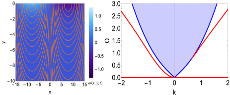
Figure 2: [Right] Bulk (blue) and boundary (red) dispersion relation. [Left] Velocity profile vector field $(v_{x}(x,y),v_{y}(x,y))$ is plotted as a streamline plot with the color density denoting the vorticity profile $\omega(x,y)$ for time $t=0$ and $k=0.20551$.

The leading term of the surface wave dispersion (20) is universal and coincides with the one obtained in Ref. abanov2018odd . However, in contrast with Ref. abanov2018odd the sub-leading in $k/k_{0}$ terms in (20) are also non-dissipative. Solutions for the velocity and density profiles and their scaling with respect to $k_{0}$ are discussed in the supplementary material SM and are shown in Figure 2. As there is an exact symmetry $\Omega(k)\to-\Omega(-k)$ due to the PT symmetry of the hydrodynamic equations with odd viscosity, we show only the $\Omega\geq 0$ part of the spectrum in Fig. 2. The left panel of Figure 2 shows the bulk vorticity profile corresponding to the chiral boundary mode. We note here that the results for large $k/k_{0}$ are expected to be less universal as in applications they can be changed by higher order gradient corrections to the hydrodynamic equations.

Discussion and conclusions. In this letter we considered a non-dissipative fluid with odd viscosity subject to the free surface boundary conditions. As the fluid dynamics is non-dissipative, the hydrodynamic equations can be obtained through the variational principle in Eqs. (5-7). The no-stress boundary condition is accounted for by the boundary action (7). The latter has a form of 1+1 action of two chiral boson fields $h$ and $\phi$ coupled to the background boundary geometry. The field $h$ describes the form of the boundary and the field $\phi$ is an auxiliary field that can be removed for the price of making the boundary action nonlocal.

The Hamiltonian structure of the fluid dynamics derived for a fluid domain with no boundary allows for an interesting Hamiltonian reduction. Imposing the Hall constraint $Q=\nu^{-1}h/m$ makes all Casimirs (8) proportional to the total mass of the fluid. The Hall constraint plays an important role in the hydrodynamics of the quantum Hall effect, and our interpretation makes this constraint very natural from the point of view of the Hamiltonian structure corresponding to the action (5-7) SM .

Within the linearized dynamics, we showed that the velocity divergence in a compressible fluid with odd viscosity generates the vortical boundary layer at the surface of the fluid. The boundary layer is necessary to satisfy the tangent no-stress boundary condition. As a result, a chiral wave with the dispersion (20) can propagate along the fluid edge even in the absence of an external confining potential. The finite compressibility of the fluid regularizes singularities at the surface even in the absence of shear viscosity.

The variational principle presented in this work is a good starting point for studying various issues related to surface excitations of fluids with broken parity. For example, one can use the action (5-7) to obtain the nonlinear surface waves in the incompressible limit by taking $c_{s}\rightarrow\infty$. In the lowest order in nonlinearity the result should match the action proposed in Ref. abanov2018free on phenomenological grounds. Even more interestingly, one could impose the Hall constraint on the action (5-7) and study the effects of odd viscosity on edge excitations of fluids similar to quantum Hall fluids. We reserve the investigation of these questions for future work.

Acknowledgments. We are grateful to Paul Wiegmann for many discussions and for careful reading and commenting on an earlier draft of this work. AGA’s research was supported by grants NSF DMR-1606591 and US DOE DESC-0017662. AGA and GMM are grateful to International Institute of Physics, Natal, Brazil for hospitality. GMM thanks Fundação de Amparo à Pesquisa do Estado de São Paulo (FAPESP) for financial support under grant 2016/13517-0. SG acknowledges support from PSC-CUNY Award. SG acknowledges Aspen Center for Physics where part of this work was carried out, which is supported by National Science Foundation grant PHY-1607611.

I Supplementary Information

II Bulk Variational Principle and Hamiltonian Structure

In this section, we present a hydrodynamic action which provides the bulk equations (1) for a compressible fluid with odd viscosity. For the brevity of notations we put the charge to mass ration $e/m\to 1$ and use the notation in Eq. (4), namely, $u_{\mu}\equiv\partial_{\mu}\theta+A_{\mu}+\alpha\partial_{\mu}\gamma$ for $\mu=0,1,2$. Let us assume the fluid domain to be the whole two-dimensional plane. The generalization to the fluid domain with free surface will be discussed in the next section. Let us consider the action:

$$S[\theta,\alpha,\gamma,\rho,v_{i}]=-\int dt\int_{\mathbb{R}^{2}}d^{2}x\left[\rho(u_{0}+v^{i}u_{i})\rho-\frac{\rho v^{i}v_{i}}{2}+\varepsilon(\rho)-\nu_{o}v_{i}\epsilon^{ij}\partial_{j}\rho\right]\,.$$ (21)

Variation of this action gives us

$$\delta S=\int dt\int d^{2}x\left[\rho\,\delta v^{i}\left(v_{i}-u_{i}+\frac{\nu_{o}}{\rho}\partial_{i}^{*}\rho\right)+(\delta\theta+\alpha\delta\gamma)\Big{(}\partial_{t}\rho+\partial_{i}(\rho v^{i})\Big{)}+\rho\,\delta\gamma\left(\partial_{t}\alpha+v^{i}\partial_{i}\alpha\right)\right.$$

$$\left.-(\rho\,\delta\alpha+\alpha\,\delta\rho)\left(\partial_{t}\gamma+v^{i}\partial_{i}\gamma\right)-\delta\rho\left(\partial_{t}\theta+A_{0}+v^{i}(\partial_{i}\theta+A_{i})-\frac{1}{2}v^{i}v_{i}+\varepsilon^{\prime}(\rho)-\nu_{o}\epsilon^{ij}\partial_{i}v_{j}\right)\right].$$ (22)

From this variation, we obtain the Clebsch parametrization of velocity given in Eq. (4), the continuity equation and the dynamics of the Clebsch potentials:

$$v_{i}=u_{i}-\nu_{o}\partial_{i}^{*}\ln\rho\,,$$ (23)

$$\partial_{t}\rho+\partial_{i}(\rho v_{i})=0\,,$$ (24)

$$\partial_{t}\alpha+v^{i}\partial_{i}\alpha=0\,,$$ (25)

$$\partial_{t}\gamma+v^{i}\partial_{i}\gamma=0\,$$ (26)

$$\partial_{t}\theta+A_{0}+v^{i}(\partial_{i}\theta+A_{i})=\frac{1}{2}v^{i}v_{i}-\varepsilon^{\prime}(\rho)+\nu_{o}\epsilon^{ij}\partial_{i}v_{j}\,.$$ (27)

Euler equation is obtained by taking the time derivative of $v_{i}$ from Eq. (4) and using the equations of motion to Clebsch potentials. Hence,

$$\partial_{t}v_{i} =\partial_{i}\partial_{t}\theta+\partial_{t}\alpha\partial_{i}\gamma+\alpha\partial_{i}\partial_{t}\gamma+\partial_{t}A_{i}-\nu_{o}\partial_{i}^{*}\partial_{t}(\ln\rho)\,,$$

$$\partial_{t}v_{i} =\partial_{i}\left[v^{j}\left(\frac{v_{j}}{2}-\partial_{j}\theta-A_{j}\right)-\varepsilon^{\prime}(\rho)+\nu_{o}\epsilon^{jk}\partial_{j}v_{k}-A_{0}\right]-v^{j}\partial_{j}\alpha\partial_{i}\gamma-\alpha\partial_{i}(v^{j}\partial_{j}\gamma)+\partial_{t}A_{i}+\nu_{o}\partial_{i}^{*}\left[\frac{1}{\rho}\partial_{j}(\rho v^{j})\right]\,,$$

$$\partial_{t}v_{i} =-\partial_{i}\left[v^{j}(\nu_{o}\partial_{j}^{*}\ln\rho+\tfrac{1}{2}v_{j})+\varepsilon^{\prime}(\rho)-\nu_{o}\omega\right]+v^{j}(\partial_{i}\alpha\partial_{j}\gamma-\partial_{j}\alpha\partial_{i}\gamma)-E_{i}+\nu_{o}v^{j}\partial_{j}\partial_{i}^{*}\ln\rho+\nu_{o}\partial_{j}\partial_{i}^{*}v^{j}+\frac{\nu_{o}}{\rho}\partial_{i}^{*}v^{j}\partial_{j}\rho\,.$$

In order to express the last line solely in terms of the fluid density and the velocity field, we must note that

$$v^{j}(\partial_{i}v_{j}-\partial_{j}v_{i})=v^{j}(\partial_{i}\alpha\partial_{j}\gamma-\partial_{j}\alpha\partial_{i}\gamma)+B\epsilon_{ij}-\nu_{o}v^{j}(\partial_{i}\partial_{j}^{*}\ln\rho-\partial_{j}\partial_{i}^{*}\ln\rho)\,,$$

and after a little bit of algebra, we end up with

$$\partial_{t}v_{i}=-v^{j}\partial_{j}v_{i}-(B\epsilon_{ij}v^{j}+E_{i})-\partial_{i}\Big{(}\varepsilon^{\prime}(\rho)-\nu_{o}\partial_{j}v^{*j}\Big{)}+\frac{\nu_{o}}{\rho}\partial_{j}\Big{(}\rho\,\partial_{i}^{*}v^{j}\Big{)}-\frac{\nu_{o}}{\rho}\partial_{i}v^{j}\partial_{j}^{*}\rho\,,$$

$$\partial_{t}v_{i}+v^{j}\partial_{j}v_{i}=-(B\epsilon_{ij}v^{j}+E_{i})-\frac{1}{\rho}\partial_{j}\left[p(\rho)\,\delta^{j}_{i}-\nu_{o}\rho\left(\partial_{i}^{*}v^{j}+\partial_{i}v^{*j}\right)\right]\,,$$ (28)

where we used the identity

$$\partial_{i}v^{j}\partial_{j}^{*}\rho=-\partial_{i}v^{*j}\partial_{j}\rho\,,$$

together with fluid pressure definition, that is, $p(\rho)=\rho\varepsilon^{\prime}(\rho)-\varepsilon(\rho)$.

II.1 Hamiltonian Structure

In the action (21), the field $v_{i}$ is a Lagrange multiplier and can be “integrated out”. Therefore, we can rewrite it as

$$S=-\int dt\int d^{2}x\left[\rho\left(\partial_{t}\theta+A_{0}+\alpha\partial_{t}\gamma+\frac{1}{2}v^{i}v_{i}\right)+\varepsilon(\rho)\right].$$ (29)

Here the velocity field $v_{i}$ is expressed in terms of Clebsch parameters by Eq. (4). We separate time derivatives and rewrite (29) as

$$S=\int dt\left\{\int d^{2}x\Big{[}-\rho\partial_{t}\theta-\rho\alpha\partial_{t}\gamma\Big{]}-H\right\}\,,$$ (30)

where the fluid Hamiltonian is given by

$$H=\int d^{2}x\left[\frac{1}{2}\rho v^{i}v_{i}+\varepsilon(\rho)+\rho A_{0}\right]\,.$$ (31)

The part of the action (30) containing time derivatives defines the Poisson algebra of the system. From the action (30), we see that $-\rho$ and $\theta$ are conjugated quantities whereas $-\rho\alpha$ is conjugated to $\gamma$. This means that we have the following Poisson brackets

$$\{\rho,\theta^{\prime}\} =-\delta(\bm{x}-\bm{x}^{\prime}),$$ (32)

$$\{\rho\alpha,\gamma^{\prime}\} =-\delta(\bm{x}-\bm{x}^{\prime}),$$ (33)

$$\{\theta,\gamma^{\prime}\} =0,$$ (34)

$$\{\rho,\rho^{\prime}\alpha^{\prime}\} =0,$$ (35)

$$\{\rho,\gamma^{\prime}\} =0,$$ (36)

$$\{\rho\alpha,\theta^{\prime}\} =0.$$ (37)

Here, for the sake of brevity, we used the notations $\rho=\rho(t,\bm{x})$, $\theta^{\prime}=\theta(t,\bm{x}^{\prime})$, etc.

It is straightforward to see that this canonical algebra is the same for fluids without odd viscosity. Namely, it is not hard to show that

$$\{\rho,\rho^{\prime}\} =0\,,$$ (38)

$$\{\rho,u_{i}^{\prime}\} =\partial_{i}\delta(\bm{x}-\bm{x}^{\prime})\,,$$ (39)

$$\{u_{i},u_{j}^{\prime}\} =\frac{\partial_{j}u_{i}-\partial_{i}u_{j}-(\partial_{j}A_{i}-\partial_{i}A_{j})}{\rho}\delta(\bm{x}-\bm{x}^{\prime})=\frac{\partial_{j}u_{i}-\partial_{i}u_{j}+\epsilon_{ij}B}{\rho}\delta(\bm{x}-\bm{x}^{\prime})\,.$$ (40)

These brackets are the same as the brackets for density and velocity fields for a fluid without odd viscosity 1997-ZakharovKuznetsov . Therefore, the presence of odd viscosity leads to nothing but a redefinition of velocity field. One can easily obtain the Poisson brackets for $\rho$ and $v_{i}=u_{i}-\nu_{o}\partial_{i}^{*}\ln\rho$ using (38-40).

The algebra (38 - 40) is well-known and admits an infinite number of Casimirs, namely,

$$F=\int d^{2}x\,\rho\,f\left(\frac{\epsilon^{ij}\partial_{i}u_{j}-B}{\rho}\right)$$ (41)

is a Casimir for any function $f$. Rewriting it in terms of vorticity $\omega=\epsilon^{ij}\partial_{i}v_{j}$, we find

$$F=\int d^{2}x\,\rho\,f(Q)\,,$$ (42)

where $Q$ is defined by Eq. (9). We can show that $\rho Q$ is a Casimir density by imposing that $f$ is a linear function of $Q$.

From Eqs. (38-40), it is straightforward to work out the explicit form of Poisson algebra in terms of $\rho$ and $v_{i}$

$$\{\rho,\rho^{\prime}\} =0\,,$$ (43)

$$\{\rho,v_{i}^{\prime}\} =\partial_{i}\delta(\bm{x}-\bm{x}^{\prime})\,,$$ (44)

$$\{v_{i},v_{j}^{\prime}\} =-Q\epsilon_{ij}\,\delta(\bm{x}-\bm{x}^{\prime})+\nu_{o}(\partial_{i}\partial_{j}^{\prime*}-\partial_{i}^{*}\partial_{j}^{\prime})\frac{\delta(\bm{x}-\bm{x}^{\prime})}{\rho}\,.$$ (45)

Hamilton equations of motion for $\rho$ and $v_{i}$ follows from

$$\dot{\rho} =\{H,\rho\},$$ (46)

$$\dot{v}_{i} =\{H,v_{i}\}+\partial_{t}A_{i}\,,$$ (47)

where the fluid Hamiltonian is given by Eq. (31). Thus,

$$\dot{\rho}=\int d^{2}x^{\prime}\,\rho^{\prime}v^{\prime i}\{v_{i}^{\prime},\rho\}=-\partial_{i}(\rho v^{i})\,,$$ (48)

and

$$\dot{v}_{i} =\partial_{t}A_{i}+\int d^{2}x^{\prime}\left[\left(\frac{1}{2}v^{\prime j}v_{j}^{\prime}+\frac{d\varepsilon^{\prime}}{d\rho^{\prime}}+A_{0}^{\prime}\right)\{\rho^{\prime},v_{i}\}+\rho^{\prime}v^{\prime j}\{v_{j}^{\prime},v_{i}\}\right]\,.$$ (49)

Substituting (44-45) after some manipulations we obtain Euler equation corresponding to the stress (2):

$$\dot{v}_{i} =-v^{j}\partial_{j}v_{i}-(E_{i}+Bv_{i}^{*})-\frac{1}{\rho}\partial_{j}\left[p\,\delta^{j}_{i}-\nu_{o}\rho\left(\partial_{i}^{*}v^{j}+\partial_{i}v^{*j}\right)\right]\,.$$ (50)

III Variational Principle with Free Surface

In this section, we generalize the bulk action (21) to account for the free edge dynamics. For that, the hydrodynamic action must provide us the continuity and Euler equations together with kinematic and dynamic boundary conditions, Eq. (3). Let us consider the case where the fluid domain is given by $y\leq h(t,x)$, thus the bulk action becomes

$$S_{bulk}=-\int dt\int\limits_{-\infty}^{\infty}dx\int\limits_{-\infty}^{h(t,x)}dy\left[\rho(u_{0}+v^{i}u_{i})-\frac{\rho v^{i}v_{i}}{2}+\varepsilon(\rho)-\nu_{o}v_{i}\epsilon^{ij}\partial_{j}\rho\right]\,.$$ (51)

To vary this action, we must remember that the boundary function $h(t,x)$ is a dynamical field. Thus, using the Leibniz integral rule, we end up with

$$\delta S_{bulk}=\iint dt\,dx\int\limits_{-\infty}^{h(t,x)} dy\left[\rho\,\delta v^{i}\left(v_{i}-u_{i}+\frac{\nu_{o}}{\rho}\partial_{i}^{*}\rho\right)+(\delta\theta+\alpha\delta\gamma)\Big{(}\partial_{t}\rho+\partial_{i}(\rho v^{i})\Big{)}+\rho\,\delta\gamma\left(\partial_{t}\alpha+v^{i}\partial_{i}\alpha\right)\right.$$

$$\;\left.-(\rho\,\delta\alpha+\alpha\,\delta\rho)\left(\partial_{t}\gamma+v^{i}\partial_{i}\gamma\right)-\delta\rho\left(\partial_{t}\theta+A_{0}+v^{i}(\partial_{i}\theta+A_{i})-\frac{1}{2}v^{i}v_{i}+\varepsilon^{\prime}(\rho)-\nu_{o}\epsilon^{ij}\partial_{i}v_{j}\right)\right]$$

$$+\iint dt\,dx\Big{\{}\rho(\delta\theta +\alpha\delta\gamma)[\partial_{t}h+v_{x}\partial_{x}h-v_{y}]-\delta h\left[\rho\alpha(\partial_{t}\gamma+v^{i}\partial_{i}\gamma)+\varepsilon(\rho)-\nu_{o}\epsilon^{ij}v_{i}\partial_{j}\rho+\rho(\partial_{t}\theta+v^{i}\partial_{i}\theta-\tfrac{1}{2}v^{i}v_{i})\right]$$

$$+\,\nu_{o} \delta\rho(v_{x}+v_{y}\partial_{x}h)\Big{\}}_{y=h(t,x)}\,.$$ (52)

Variations of fields on the bulk are the same as in the previous section, hence they provide the same bulk equations. Thus, this action variation on bulk equations of motion becomes

$$\delta S_{bulk}\Big{|}_{on\;EoM}= \iint dt\,dx\Big{\{}\rho(\delta\theta+\alpha\delta\gamma)[\partial_{t}h+v_{x}\partial_{x}h-v_{y}]-\delta h\Big{[}p(\rho)-\nu_{o}\epsilon^{ij}\partial_{j}(\rho v_{j})\Big{]}$$

$$+\,\nu_{o}\delta\rho(v_{x}+v_{y}\partial_{x}h)\Big{\}}_{y=h(t,x)}\,.$$ (53)

Variations of $\theta$ and $\gamma$ on the edge give us the kinematic boundary condition, that is,

$$\partial_{t}h+v_{x}\Big{|}_{y=h}\partial_{x}h-v_{y}\Big{|}_{y=h}=0\,.$$ (54)

However, variation over $\rho$ on the boundary states that the tangent velocity vanishes at the edge, that is, $v_{x}+v_{y}\partial_{x}h=0$ and variation over $h$ states that

$$\Big{[}p(\rho)-\nu_{o}\epsilon^{ij}\partial_{j}(\rho v_{j})\Big{]}_{y=h}=0\,.$$ (55)

Obviously, these are not the no-stress boundary conditions from Eq.(3). Therefore, we must add purely boundary terms to the full action. Such boundary action can be described as

$$S_{edge}=-\nu_{o}\iint dtdx\left[\tilde{\rho}\partial_{t}h\partial_{x}h+\partial_{t}\phi\partial_{x}\phi-2\partial_{t}\phi\sqrt{\tilde{\rho}\left(1+(\partial_{x}h)^{2}\right)}\right]\,,$$ (56)

where we introduced the density boundary field $\tilde{\rho}(t,x)\equiv\rho\big{(}t,x,h(t,x)\big{)}$ and the field $\phi(t,x)$ as an independent boundary field (does not depend on $h$). To vary the edge action (56), we must take into account that the variations and derivatives of the boundary density $\tilde{\rho}$ are related to the boundary values of the variation of the bulk density $\rho$ in the following way:

$$\delta\tilde{\rho} =\delta\rho\big{|}_{y=h}+\delta h\,\partial_{y}\rho\big{|}_{y=h}\,,$$

$$\partial_{t}\tilde{\rho} =\partial_{t}\rho\big{|}_{y=h}+\partial_{t}h\,\partial_{y}\rho\big{|}_{y=h}\,,$$

$$\partial_{x}\tilde{\rho} =\partial_{x}\rho\big{|}_{y=h}+\partial_{x}h\,\partial_{y}\rho\big{|}_{y=h}\,.$$

Hence,

$$\delta S_{edge}=\nu_{o}\iint dtdx\left\{\delta\rho\left(\frac{\partial_{t}\phi}{\sqrt{\rho}}\sqrt{1+(\partial_{x}h)^{2}}-\partial_{t}h\partial_{x}h\right)+2\delta\phi\left[\partial_{t}\partial_{x}\phi-\frac{\sqrt{\rho}\,\partial_{x}h\,\partial_{x}\partial_{t}h}{\sqrt{1+(\partial_{x}h)^{2}}}-\frac{\partial_{t}\rho+\partial_{t}h\partial_{y}\rho}{2\sqrt{\rho}}\sqrt{1+(\partial_{x}h)^{2}}\right]\right.$$

$$+\left.\delta h\left[2\rho\,\partial_{x}\partial_{t}h+\partial_{t}\rho\partial_{x}h+\partial_{t}h\partial_{x}\rho+\partial_{t}h\partial_{x}h\partial_{y}\rho-2(\partial_{x}+\partial_{x}h\partial_{y})\left(\frac{\partial_{t}\phi\partial_{x}h\,\sqrt{\rho}}{\sqrt{1+(\partial_{x}h)^{2}}}\right)+\frac{\partial_{t}\phi\partial_{y}\rho}{\sqrt{\rho}}\sqrt{1+(\partial_{x}h)^{2}}\right]\right\}_{y=h}\,.$$ (57)

Combining the terms of $\delta\rho$ taken at the boundary from both bulk and boundary actions, we obtain that

$$\left[v_{x}+v_{y}\partial_{x}h-\partial_{x}h\partial_{t}h+\frac{\partial_{t}\phi}{\sqrt{\rho}}\sqrt{1+(\partial_{x}h)^{2}}\right]_{y=h}=0.$$ (58)

Using the kinematic boundary condition, we can parametrize $\partial_{t}\phi$ in terms of the hydrodynamic fields $(\rho,v_{x},h)$.

$$\partial_{t}\phi=-\left[v_{x}\sqrt{\rho\big{(}1+(\partial_{x}h)^{2}\big{)}}\right]_{y=h}.$$ (59)

Plugging the kinematic boundary condition, Eq. (54), together with Eq. (59) into the equation of motion for $\phi$, we get that

$$\left[-\big{(}\partial_{x}+\partial_{x}h\partial_{y}\big{)}\left(v_{x}\sqrt{\rho\big{(}1+(\partial_{x}h)^{2}\big{)}}\right)-\frac{\partial_{x}h\,\partial_{x}\partial_{t}h\sqrt{\rho}}{\sqrt{1+(\partial_{x}h)^{2}}}-\frac{\partial_{t}\rho+(v_{y}-v_{x}\partial_{x}h)\partial_{y}\rho}{2\sqrt{\rho}}\sqrt{1+(\partial_{x}h)^{2}}\right]_{y=h}=0,$$

$$\left[\frac{\partial_{t}\rho+v_{x}\partial_{x}\rho+v_{y}\partial_{y}\rho}{2\sqrt{\rho}}+\sqrt{\rho}\big{(}\partial_{x}v_{x}+\partial_{x}h\partial_{y}v_{x}\big{)}+\frac{v_{x}\partial_{x}h\partial_{x}^{2}h\sqrt{\rho}}{1+(\partial_{x}h)^{2}}+\frac{\partial_{x}h\sqrt{\rho}}{1+(\partial_{x}h)^{2}}\big{(}\partial_{x}+\partial_{x}h\partial_{y}\big{)}\Big{(}v_{y}-v_{x}\partial_{x}h\Big{)}\right]_{y=h}=0,$$

$$\left[-\frac{1+(\partial_{x}h)^{2}}{2}(\partial_{x}v_{x}+\partial_{y}v_{y})+\big{(}\partial_{x}v_{x}+\partial_{x}h\partial_{y}v_{x}\big{)}+\partial_{x}h\big{(}\partial_{x}v_{y}+\partial_{x}h\partial_{y}v_{y}\big{)}\right]_{y=h}=0,$$

$$\Bigg{[}\big{(}1-(\partial_{x}h)^{2}\big{)}(\partial_{x}v_{x}-\partial_{y}v_{y})+2\partial_{x}h\big{(}\partial_{x}v_{y}+\partial_{y}v_{x}\big{)}\Bigg{]}_{y=h}=0.$$ (60)

One can show with few lines of algebra that the term in the left hand side of Eq. (60) is proportional to the tangent component of the dynamic boundary condition, that is,

$$n_{i}s_{j}T^{ij}\Big{|}_{y=h}=0\,,$$ (61)

where $s_{j}$ are the components of the edge tangent vector.

Finally, let us turn our attention to the variation with respect to $h$. From the bulk action, we obtain the left hand side of Eq. (55). Combining (53) with (57) and using Eq.(59), we obtain for the total variation with respect to $h$:

$$\left[\frac{p}{\nu_{o}}-\epsilon^{ij}\partial_{i}(\rho v_{j})+2\rho\,\partial_{x}\partial_{t}h+\partial_{t}\rho\partial_{x}h+\partial_{t}h\partial_{x}\rho+\partial_{y}\rho\left(\partial_{t}h\partial_{x}h-v_{x}-v_{x}(\partial_{x}h)^{2}\right)+2(\partial_{x}+\partial_{x}h\partial_{y})\left(\rho v_{x}\partial_{x}h\right)\right]_{y=h}=0\,,$$

$$\left[\frac{p}{\nu_{o}}-\rho\,\partial_{x}h(\partial_{x}v_{x}+\partial_{y}v_{y})+\rho\,(\partial_{y}v_{x}-\partial_{x}v_{y}+2\partial_{x}\partial_{t}h)-2\rho\,\partial_{x}h(\partial_{x}v_{x}+\partial_{x}h\partial_{y}v_{x})-2\rho\,v_{x}\partial_{x}^{2}h\right]_{y=h}=0\,,$$

$$\Bigg{[}p-\nu_{o}\rho\,(\partial_{y}v_{x}+\partial_{x}v_{y})+\nu_{o}\rho\,\partial_{x}h(\partial_{x}v_{x}-\partial_{y}v_{y})\Bigg{]}_{y=h}=\sqrt{1+(\partial_{x}h)^{2}}\;n^{i}T_{iy}\Big{|}_{y=h}=0\,.$$ (62)

This condition together with (61) implies that both component of the stress at the surface are vanishing $n_{i}T^{ij}=0$ and we recovered both dynamical boundary conditions.

To conclude this section, we showed that the action given by the sum of the bulk term (51) and of the boundary term (56) reproduces both bulk equations of motion and proper boundary conditions for the compressible two-dimensional fluid with odd viscosity and free surface. This action can be used to derive the Hamiltonian structure for the fluid with free surface. We will leave this problem for future.

IV Linearized solutions

In this section, we provide the derivation details of the linear surface wave dispersion and the corresponding density and velocity profiles. In the following, we express all wavevectors in units of $k_{0}=c_{s}/\nu_{o}$, and frequencies in units of $\Omega_{0}=\nu_{o}k_{0}^{2}$. Substituting the density and velocity (18) into the the linearized dynamical boundary conditions (17) we obtain,

$$\sum_{\alpha=1}^{2}A_{\alpha}f_{\alpha}(k,\Omega)=0,\quad \sum_{\alpha=1}^{2}A_{\alpha}g_{\alpha}(k,\Omega)=0$$ (63)

$$f_{\alpha}(k,\Omega)=\left(1+\frac{2m_{\alpha}\Omega k}{k^{2}-m^{2}_{\alpha}}-(m_{\alpha}^{2}+k^{2})\right), \quad g_{\alpha}(k,\Omega)=\left(\Omega\frac{k^{2}+m_{\alpha}^{2}}{k^{2}-m^{2}_{\alpha}}-2m_{\alpha}k\right)$$ (64)

These two equations define the eigenvalue problem for finding $\Omega$ and the corresponding amplitudes $A_{1,2}$. The decay rates $m_{\alpha}$ are subject to the condition $\operatorname{Re}(m_{\alpha})>0$ and are given by the bulk dispersion relation Eq. (13), that is $m_{\alpha}^{2}-k^{2}=\frac{1\pm\sqrt{1+4\Omega^{2}}}{2}$ for $\alpha=1,2$, respectively. It is important to know that the system of equations (63) and the relation (13) have exact PT symmetry $\Omega(k)=-\Omega(-k)$. The surface wave dispersion is found solving the compatibility condition of equations (63):

$$f_{2}(k,\Omega(k))g_{1}(k,\Omega(k))-f_{1}(k,\Omega(k))g_{2}(k,\Omega(k))=0\,.$$ (65)

The solution has PT symmetry $\Omega(k)=-\Omega(-k)$ and is plotted in Fig. 2, for $\Omega>0$.

To obtain the solutions in two limits, i.e., $k\ll 1$ and $k\gg 1$, analytically, we write $\Omega(k)=\sum_{j}a_{j}k^{j}$. Substituting this form into Eq. 65 and expanding it in the powers of $k$ we can find $a_{j}$ by setting the coefficients for each power to zero. The first three terms can be written as,

$$\Omega \approx-2\left(k^{2}-k^{3}+k^{4}\right)+O(k^{5}),\qquad\quad\,\,\text{for}\,\,k\ll 1\,,$$ (66)

$$\Omega \approx-\sqrt{2}k+\frac{1}{4\sqrt{2}}\frac{1}{k}+\frac{1}{8}\frac{1}{k^{2}}+O(k^{-3}),\;\,\,\text{for}\,\,k\gg 1\,.$$ (67)

For $k\approx 0.650551$, another counter propagating surface mode emanates out of the bulk continuum

$$\Omega \approx\sqrt{2}k-\frac{1}{4\sqrt{2}}\frac{1}{k}-\frac{1}{8}\frac{1}{k^{2}}+O(k^{-3}),\;\,\,\text{for}\,\,k\geq 0.650551\,.$$ (68)

Remarkably, the dispersion of this mode is just opposite in sign to the dispersion (67) to all orders in the $1/k$ expansion and differs from it only due to non-perturbative corrections in, giving rise to the existence of the vortical boundary layer.

Let us now focus on the long wavelength limit $k\ll 1$. Using Eq. (66), we solve Eq. (63) for the amplitudes $A_{1,2}$. Plugging it into Eq. (18) and restoring the dimensions, we end up with

$$n=-i\frac{A}{c_{s}}\left(2\frac{k}{k_{0}}e^{ky}-e^{k_{0}y}\right)e^{ikx-i\Omega t},\quad v_{x}=iA\left(e^{ky}-e^{k_{0}y}\right)e^{ikx-i\Omega t},\quad v_{y}=A\left(e^{ky}-\frac{k}{k_{0}}e^{k_{0}y}\right)e^{ikx-i\Omega t}\,,$$ (69)

where $A$ is a free parameter defining the overall size of the wave. For completeness, we also give an expression for the height of the surface $h=-\frac{iA}{2\nu_{o}k^{2}}e^{ikx-i\Omega t}$ for $k\ll k_{0}$.

The vorticity corresponding to Eq. (69) is given to the leading order by

$$\omega\approx Ak_{0}e^{k_{0}y}e^{ikx-i\Omega t}\,.$$ (70)

Let us consider the incompressible limit of these linearized solutions. We fix the wave vector $k$ and the amplitude of the vertical velocity $v_{y}$ to be $A$. We then send $c_{s}\to\infty$ ($k_{0}\to\infty$). We find that the density is constant ($n\to 0$) and the velocities $v_{x},v_{y}$ are finite in this limit everywhere near the boundary, while the vorticity (70) diverges near the surface $\omega\sim k_{0}\sim c_{s}$. Interestingly, the tangent velocity $v_{x}$ taken exactly at the surface $y=0$ vanishes in linear approximation and can have only values of higher order in the amplitude $A$ (beyond the linear approximation considered here). However, at finite depth of the order of $\delta=1/k_{0}\to 0$ the tangent velocity is finite and is of the order of $A$. Essentially, one can say that in the incompressible limit the tangent velocity has a finite discontinuity across the infinitesimal vortical boundary layer.

We plot the linearized bulk velocity and vorticity profiles for different values of $k$ in Fig. 3. The velocity profile given by the real parts of (69) are represented in the form of streamlines. The vorticity is plotted as color density plot in the background of the velocity streamline plots. The odd viscosity dominates the flow for small negative $k$ shown in $k=-0.2$. The dimensionful surface dispersion for small negative $k$ is of the form $\Omega\sim-2\nu_{o}k|k|$. For intermediate and large negative values of $k$ the odd viscosity effects are suppressed and the dimensionful dispersion relation is of the form $\Omega\sim-\sqrt{2}c_{s}k$ which is independent of odd viscosity. Another evidence of suppression of parity breaking effects at large $k$ is shown by the emergence of a counter propagating mode for the $k\geq 0.65501$. For the critical value of $k\approx 0.65501$, we see that the vorticity penetrates deep into the bulk due to the vanishing of the decay rate $m$ becoming a bulk mode. Since the bulk and boundary dispersion cross at this point, the disappearance of the boundary mode at low $k$ can be understood as due to a hybridization with the bulk.

In the $k\gg k_{0}$ limit the dispersion relation is of the form $\Omega=\pm\sqrt{2}c_{s}k$. The density and velocity profiles in this limit are of the form,

$$n=\frac{2\sqrt{2}iA}{c_{s}}e^{ikx-i\Omega t}e^{|k|y},\quad v_{x}=-2iAe^{ikx-i\Omega t}e^{|k|y},\quad v_{y}=2Ae^{ikx-i\Omega t}e^{|k|y}$$ (71)

The vorticity for this case is confined within the length $1/k\ll 1/k_{0}$ and is given by,

$$\omega=4iAke^{ikx-i\Omega t}e^{|k|y}.$$ (72)

Even though the dispersion and the profile seems to be independent of odd viscosity $\nu_{o}$, the existence of a localized boundary mode is exclusively due to the presence of $\nu_{o}$. This is due to the fact that the tangent boundary condition resulting in the vortical boundary layer does not depend on the scale of the odd viscosity. However, a nonvanishing tangent boundary condition is solely a consequence of a non-zero odd viscosity.

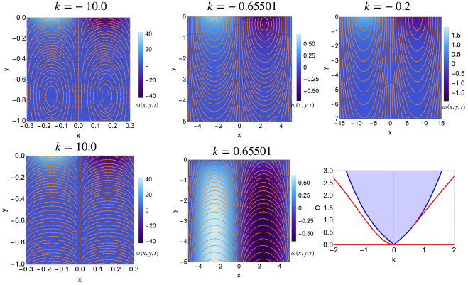
Figure 3: Velocity streamlines overlaid over the vorticity profile are shown for different values of $k=\pm 10.0,\pm 0.65501,-0.2$. The lower right panel shows the dispersion of bulk (blue) and surface (red) waves.

References

- (1) J. Avron. Odd viscosity. Journal of statistical physics, 92, 543–557 (1998).
- (2) J. Avron, R. Seiler, and P. G. Zograf. Viscosity of quantum Hall fluids. Physical review letters, 75, 697 (1995).
- (3) I. Tokatly. Magnetoelasticity theory of incompressible quantum Hall liquids. Physical Review B, 73, 205340 (2006).
- (4) I. Tokatly and G. Vignale. New collective mode in the fractional quantum Hall liquid. Physical review letters, 98, 026805 (2007).
- (5) I. Tokatly and G. Vignale. Erratum: Lorentz shear modulus of a two-dimensional electron gas at high magnetic field [Phys. Rev. B 76, 161305 (R)(2007)]. Physical Review B, 79, 199903 (2009).
- (6) N. Read. Non-Abelian adiabatic statistics and Hall viscosity in quantum Hall states and p x+ i p y paired superfluids. Physical Review B, 79, 045308 (2009).
- (7) F. Haldane. Geometrical description of the fractional quantum Hall effect. Physical review letters, 107, 116801 (2011).
- (8) F. Haldane. Self-duality and long-wavelength behavior of the Landau-level guiding-center structure function, and the shear modulus of fractional quantum Hall fluids. arXiv preprint arXiv:1112.0990 (2011).
- (9) C. Hoyos and D. T. Son. Hall viscosity and electromagnetic response. Physical review letters, 108, 066805 (2012).
- (10) B. Bradlyn, M. Goldstein, and N. Read. Kubo formulas for viscosity: Hall viscosity, Ward identities, and the relation with conductivity. Physical Review B, 86, 245309 (2012).
- (11) B. Yang, Z. Papić, E. Rezayi, R. Bhatt, and F. Haldane. Band mass anisotropy and the intrinsic metric of fractional quantum Hall systems. Physical Review B, 85, 165318 (2012).
- (12) A. G. Abanov. On the effective hydrodynamics of the fractional quantum Hall effect. Journal of Physics A: Mathematical and Theoretical, 46, 292001 (2013).
- (13) T. L. Hughes, R. G. Leigh, and O. Parrikar. Torsional anomalies, Hall viscosity, and bulk-boundary correspondence in topological states. Physical Review D, 88, 025040 (2013).
- (14) C. Hoyos. Hall viscosity, topological states and effective theories. International Journal of Modern Physics B, 28, 1430007 (2014).
- (15) M. Laskin, T. Can, and P. Wiegmann. Collective field theory for quantum Hall states. Physical Review B, 92, 235141 (2015).
- (16) T. Can, M. Laskin, and P. Wiegmann. Fractional quantum Hall effect in a curved space: gravitational anomaly and electromagnetic response. Physical review letters, 113, 046803 (2014).
- (17) T. Can, M. Laskin, and P. B. Wiegmann. Geometry of quantum Hall states: Gravitational anomaly and transport coefficients. Annals of Physics, 362, 752–794 (2015).
- (18) S. Klevtsov and P. Wiegmann. Geometric adiabatic transport in quantum Hall states. Physical review letters, 115, 086801 (2015).
- (19) S. Klevtsov, X. Ma, G. Marinescu, and P. Wiegmann. Quantum Hall effect and Quillen metric. Communications in Mathematical Physics, 349, 819–855 (2017).
- (20) A. Gromov and A. G. Abanov. Density-curvature response and gravitational anomaly. Physical review letters, 113, 266802 (2014).
- (21) A. Gromov, G. Y. Cho, Y. You, A. G. Abanov, and E. Fradkin. Framing anomaly in the effective theory of the fractional quantum hall effect. Physical review letters, 114, 016805 (2015).
- (22) A. Gromov, K. Jensen, and A. G. Abanov. Boundary effective action for quantum Hall states. Physical review letters, 116, 126802 (2016).
- (23) T. Scaffidi, N. Nandi, B. Schmidt, A. P. Mackenzie, and J. E. Moore. Hydrodynamic electron flow and Hall viscosity. Physical review letters, 118, 226601 (2017).
- (24) L. V. Delacrétaz and A. Gromov. Transport Signatures of the Hall Viscosity. Phys. Rev. Lett., 119, 226602 (2017).
- (25) P. Alekseev. Negative magnetoresistance in viscous flow of two-dimensional electrons. Physical review letters, 117, 166601 (2016).
- (26) F. M. Pellegrino, I. Torre, and M. Polini. Nonlocal transport and the Hall viscosity of two-dimensional hydrodynamic electron liquids. Physical Review B, 96, 195401 (2017).
- (27) J. Korving, H. Hulsman, H. Knaap, and J. Beenakker. Transverse momentum transport in viscous flow of diatomic gases in a magnetic field. Physics Letters, 21, 5–7 (1966).
- (28) H. Knaap and J. Beenakker. Heat conductivity and viscosity of a gas of non-spherical molecules in a magnetic field. Physica, 33, 643–670 (1967).
- (29) J. Korving, H. Hulsman, G. Scoles, H. Knaap, and J. Beenakker. The influence of a magnetic field on the transport properties of gases of polyatomic molecules;: Part I, Viscosity. Physica, 36, 177–197 (1967).
- (30) H. Hulsman, E. Van Waasdijk, A. Burgmans, H. Knaap, and J. Beenakker. Transverse momentum transport in polyatomic gases under the influence of a magnetic field. Physica, 50, 53–76 (1970).
- (31) D. Banerjee, A. Souslov, A. G. Abanov, and V. Vitelli. Odd viscosity in chiral active fluids. Nature Communications, 8, 1573 (2017).
- (32) A. Souslov, K. Dasbiswas, M. Fruchart, S. Vaikuntanathan, and V. Vitelli. Topological waves in fluids with odd viscosity. Physical Review Letters, 122, 128001 (2019).
- (33) V. Soni, E. Bililign, S. Magkiriadou, S. Sacanna, D. Bartolo, M. J. Shelley, and W. Irvine. The free surface of a colloidal chiral fluid: waves and instabilities from odd stress and Hall viscosity. arXiv preprint arXiv:1812.09990 (2018).
- (34) P. Wiegmann and A. G. Abanov. Anomalous hydrodynamics of two-dimensional vortex fluids. Physical review letters, 113, 034501 (2014).
- (35) X. Yu and A. S. Bradley. Emergent non-eulerian hydrodynamics of quantum vortices in two dimensions. Physical review letters, 119, 185301 (2017).
- (36) A. Bogatskiy and P. Wiegmann. Edge Wave and Boundary Layer of Vortex Matter. Phys. Rev. Lett., 122, 214505 (2019).
- (37) A. Bogatskiy. Vortex flows on closed surfaces. arXiv preprint arXiv:1903.07607 (2019).
- (38) C. Hoyos, S. Moroz, and D. T. Son. Effective theory of chiral two-dimensional superfluids. Physical Review B, 89, 174507 (2014).
- (39) A. Berdyugin, S. Xu, F. Pellegrino, R. K. Kumar, A. Principi, I. Torre, M. B. Shalom, T. Taniguchi, K. Watanabe, I. Grigorieva, et al. Measuring hall viscosity of graphene’s electron fluid. Science, page eaau0685 (2019).
- (40) S. Ganeshan and A. G. Abanov. Odd viscosity in two-dimensional incompressible fluids. Physical Review Fluids, 2, 094101 (2017).
- (41) A. Abanov, T. Can, and S. Ganeshan. Odd surface waves in two-dimensional incompressible fluids. SciPost Physics, 5, 010 (2018).
- (42) G. George. Stokes. On the theory of oscillatory waves. Transactions of the Cambridge Philosophical Society, 8, 441–455 (1847).
- (43) This dispersion is an approximation to deep water waves.
- (44) H. Lamb. Hydrodynamics. Cambridge university press (1932).
- (45) Both the fluid velocity and vorticity inside the layer are finite in the limit producing small damping of the surface waves vanishing in the limit of an ideal fluid . The damping rate is given by a well known result quadratic in the wave vector lamb1932hydrodynamics .
- (46) In this work we neglect all thermal and dissipative effects and energy conservation is a direct consequence of mass and momentum conservation. Indeed, it is easy to check that in the absence of external electric field the energy density with is locally conserved.
- (47) The fluid with is known as barotropic fluid. More generally, one should include entropy density field and write . In this case the conservation of energy equation should be added to (1).
- (48) Changing the definition of velocity by gradients is known as hydrodynamic frame redefinition.
- (49) S. Moroz and D. T. Son. Bosonic superfluid on lowest Landau level. arXiv preprint arXiv:1901.06088 (2019).
- (50) Although the fluid Hamiltonian is only a function of mass density and flow velocity, the Poisson algebra between these quantities is degenerate, due to the existence of Casimirs. To overcome this difficulty, the phase space must be enlarged. In the enlarged phase space, density and Clebsch potentials become canonical variables.
- (51) V. E. Zakharov and E. Kuznetsov. Hamiltonian formalism for nonlinear waves. Usp Fiz Nauk+, 167, 1137–1167 (1997).
- (52) See Supplemental Material for details of the derivations.
- (53) M. Stone. Superfluid dynamics of the fractional quantum Hall state. Physical Review B, 42, 212 (1990).
- (54) For given and , Eq. (13) is a fourth order polynomial for with four roots, only two of which have positive real part for or .
- (55) A. G. Abanov and G. M. Monteiro. Free surface variational principle for an incompressible fluid with odd viscosity. Phys Rev Lett, 122, 154501 (2019).