Optimal finite element error estimates for an optimal control problem governed by the wave equation with controls of bounded variation.

Abstract

This work discusses the finite element discretization of an optimal control problem for the linear wave equation with time-dependent controls of bounded variation. The main focus lies on the convergence analysis of the discretization method. The state equation is discretized by a space-time finite element method. The controls are not discretized. Under suitable assumptions optimal convergence rates for the error in the state and control variable are proven. Based on a conditional gradient method the solution of the semi-discretized optimal control problem is computed. The theoretical convergence rates are confirmed in a numerical example. BV-Functions; optimal control of a wave equation; error bounds; finite elements.

AMS subject classifications: 26A45, 49J20, 49M25, 65N15, 65N30.

1 Introduction

In this paper we derive a priori error estimates for a finite element discretization of the following optimal control problem governed by the linear wave equation:

$$(P)\left\{\begin{matrix}&\min_{u\in BV(0,T)^{m}}\frac{1}{2}\|y_{u}-y_{d}\|_{L^{2}(\Omega_{T})}^{2}+\sum\nolimits_{j=1}^{m}\alpha_{j}\|D_{t}u_{j}\|_{M(I)}=:J(y,u)\\ \\ \text{subject to }&(\mathcal{W})\left\{\begin{matrix}\partial_{tt}y-\Delta y=f=\sum\nolimits_{j=1}^{m}u_{j}g_{j}&\text{ in }&I\times\Omega\\ y=0&\text{ on }&I\times\partial\Omega\\ (y,\partial_{t}y)=(y_{0},y_{1})&\text{ in }&\{0\}\times\Omega,\end{matrix}\right.\end{matrix}\right.$$

where $\Omega\subset\mathbb{R}^{n}$, with $n\in\{1,2,3\}$, is a convex, polygonal/polyhedral bounded domain. For $T\in(0,\infty)$ we denote $I=(0,T)$. The desired state $y_{d}$ is assumed to satisfy $y_{d}\in C^{1}(\overline{I};L^{2}(\Omega))$. The time depending controls $u$ are given by $u=(u_{1},\cdots,u_{m})\in BV(0,T)^{m}$, and $BV(0,T)^{m}$ is endowed with the norm $\|u\|_{BV(I)^{m}}=\sum\nolimits_{j=1}^{m}(\|u_{j}\|_{L^{1}(I)^{m}}+\|D_{t}u_{j}\|_{M(I)})$. Here $M(I)$ is the space of Borel measures, endowed with the total variation norm $\|\cdot\|_{M(I)}$. Further, let $(g_{j})_{j=1}^{m}\subset L^{\infty}(\Omega)\smallsetminus\{0\}$ with pairwise disjoint supports and $\alpha_{j}>0$. The initial data is chosen as $(y_{0},y_{1})\in H^{1}_{0}(\Omega)\times L^{2}(\Omega)$. Finally, we set $\Omega_{T}:=I\times\Omega$.

In this work we focus on controls of bounded variation in time. By using the total variation norm in $(P)$, sparsity in the derivative of the controls is promoted, resulting in locally constant controls. This is in particular the case if the derivative of the optimal control is a linear combination of Dirac functions. Optimal control problems with $BV$-controls are already analyzed for elliptic and parabolic state equations in [6, 4, 13, 7, 8, 10].

Since our article deals with a priori error estimates of a finite element discretization for the control problem $(P)$, we briefly discuss previous works on error estimates for PDE control problems with $BV$-controls. In [4] the authors discretize the time-dependent $BV-$controls by cellwise constant functions. The state equation is discretized by piecewise constant finite elements in time and linear continuous finite elements in space. Based on this discretization approach, the authors show that the optimal value of the cost functional and the states converge with an order of $\sqrt{\tau}$ in time and linear in space. However, numerical experiments in [4] indicate better results. In [13] the authors analyze a finite element discretization of an elliptic control problem with $BV$-controls in a one dimensional setting. As in our case the controls are not discretized. The main contribution of this work is the derivation of optimal error estimates for the control variable in the $L^{1}$-norm. Their analysis relies on the one dimensional setting and on structural assumption on the optimal adjoint state which guarantee that the optimal control is piecewise constant and has finitely many jumps. In our work we derive similar optimal error estimates also for the problem with a multi-dimensional wave equation and our analysis relies partially on techniques developed in the former work.

Next we briefly address the difficulties in the derivation of finite element error estimates for optimal control problems with PDEs and $BV$-controls. Standard techniques for the derivation of finite element error estimates, see e.g. [9], cannot be applied due to the non-smoothness of the cost functional and the non-reflexivity of $BV(I)$. In the last years several papers concerning the derivation of finite element error estimates for optimal control problems with measure-valued controls appeared, see e.g. [15, 18]. Using the fact that for one dimensional controls, $BV(I)$ is isomorphic to $M(I)\times\mathbb{R}$, some techniques from these works are used to derive error estimates for $BV$-controls. Finally, we mention that the literature on finite element error estimates for optimal control problems governed by the wave equation is very limited. To our knowledge the only existing work in this context is [18] which uses the space-time finite element discretization developed and analyzed in [19]. Our work also relies on this discretization method for the state equation and its error analysis.
The main contribution of this work is the derivation of an optimal error estimate of the control variable in the $L^{1}(I)$-norm and of the state variable in the $L^{2}(\Omega_{T})$-norm. The state equation is discretized by a space-time finite element method with piecewise linear and continuous Ansatz- and test-functions from [19]. The weak formulation of the discrete state equation is augmented with a stabilization term involving the stabilization parameter $\sigma$. Stability of the method depends on the value of this parameter. Moreover, for certain values of this parameter the method is equivalent to wellknown time stepping schemes, like the Crank-Nicolson scheme or the Leap-Frog scheme. The $BV$-controls are not discretized. Due to fact that the controls are only time-dependent the problem under consideration can be reformulated as a measure-valued control problem. Based on the optimality conditions of the continuous and discrete optimal control problem the error in the state variable in the $L^{2}(\Omega_{T})$-norm can be represented in terms of the finite element error of the state and adjoint state equation in the $L^{2}(\Omega_{T})$-norm resp. the $L^{\infty}(I;L^{2}(\Omega))$ as well as the error in the control variable in the $L^{1}(I)$-norm. The convergence rates for the finite element error of the state and adjoint state are obtained from [19]. Under the assumption that the continuous and time depending functions

$$\bar{p}_{1,i}:t\mapsto-\int\nolimits^{T}_{t}\int\nolimits_{\Omega}\overline{p}g_{i}~{}dx~{}ds,\text{ for }i=1,\cdots,m,$$

where $\overline{p}$ is the optimal adjoint state, $\bar{p}_{1,i}$ is bounded by $\pm\alpha_{i}$, is equal to $\alpha_{i}$ at finitely many points in $I$, and the second derivatives of $\bar{p}_{1,i}$ do not vanish in these points (see (A1) and (A2)), it follows that the continuous optimal control is piecewise constant and has finitely many jumps. To obtain this information about the form of the optimal BV control, using $\bar{p}_{1,i}$, is particularly elementary because we consider controls in one dimension. Furthermore, it is proven that the solution of the discrete problem has the same number of jumps which are located close to the jumps of the continuous optimal control. Using these properties the error of the optimal control in the $L^{1}(I)$-norm is estimated in terms of the error of the state variable in the $L^{2}(\Omega_{T})$-norm. Using a bootstrapping argument optimal rates for the error in the state and control variable as well as for the optimal value of the cost are proven. These rates are confirmed by a numerical example with known solution.
This work has the following structure. Section 2 summarizes several needed results on the regularity of weak solutions of the wave equation. In section 3 the space-time finite element method from [19] is presented. Moreover, important stability results as well as a priori error estimates are stated. Section 4 deals with the reformulation of the $BV$-control problem as a measure-valued control problem and with the analysis of this problem. In particular, first order optimality conditions are derived. The next section 5 is concerned with discretization of the control problem. It is based on the mentioned space-time finite element method and the variational discretization concept. In section 6 the error estimates for the optimal state and control variable as well as the optimal functional value are derived. Finally, in section 7 a generalized conditional gradient method is introduced which applicable in the context of controls which are not discretized. Based on this method a problem with known solution is solved and the theoretical error estimates are confirmed.

2 Preliminaries on the Wave Equation

We consider $\Omega\subset\mathbb{R}^{d}$, $d=1,2,3$ as convex, polygonal/polyhedral domain. Let $\{\lambda_{k}\}_{k\in\mathbb{N}}$ be the non-decreasing eigenvalues of the Laplace operator $-\Delta$ with homogeneous boundary conditions and let $\{\mu_{k}\}_{k\in\mathbb{N}}$ be the corresponding system of eigenfunctions, which are orthonormal complete in $L^{2}(\Omega)$, and orthogonal complete in $H^{1}_{0}(\Omega)$. Hence, let us introduce for $\alpha\geq 0$ the Hilbert spaces

$$\mathbb{H}^{\alpha}=\left\{w\in L^{2}(\Omega)\left|\|w\|_{\mathbb{H}^{\alpha}}^{2}:=\sum\nolimits_{k\geq 1}\left(\lambda^{(k)}\right)^{\alpha}\left\langle w,\mu_{k}\right\rangle_{L^{2}(\Omega)}^{2}<\infty\right.\right\}.$$

For $\alpha=0,1$ we get $L^{2}(\Omega)$ respectively $H^{1}_{0}(\Omega)$. The convexity of $\Omega$ implies that $\mathbb{H}^{2}=H^{2}(\Omega)\cap H^{1}_{0}(\Omega)$. In general holds $\mathbb{H}^{\alpha}\hookrightarrow\mathbb{H}^{\beta}$ for $\alpha\geq\beta$. We denote the dual space of $\mathbb{H}^{\alpha}$ by $\mathbb{H}^{-\alpha}$. Next we introduce the weak solution of the wave equation with the forcing function $f$, initial displacement $y_{0}$, and initial velocity $y_{1}$.

Definition 1.

([14], Chap.IV, Sec.4)
Let $(f,y_{0},y_{1})\in L^{1}(I;L^{2}(\Omega))\times H^{1}_{0}(\Omega)\times L^{2}(\Omega)$. We call a function $y\in C(\overline{I};H^{1}_{0}(\Omega))$ with $\partial_{t}y\in C(\overline{I};L^{2}(\Omega))$ a weak solution of $(\mathcal{W})$ , if

$$\int_{0}^{T}-(\partial_{t}y,\partial_{t}\eta)_{L^{2}(\Omega)}+(\nabla y,\nabla\eta)_{L^{2}(\Omega)}~{}dt=(y_{1},\eta(0))_{L^{2}(\Omega)}+\int_{0}^{T}(f,\eta)_{L^{2}(\Omega)}~{}dt$$ (1)

for any $\eta\in L^{1}(I;H^{1}_{0}(\Omega))$ such that $\partial_{t}\eta\in L^{1}(I;L^{2}(\Omega))$, $\eta|_{t=T}=0$, and $y$ satisfies the initial condition $y|_{t=0}=y_{0}$.

For the following existence and regularity results of weak solutions of the wave equation we refer to [19, Proposition 1.1., 1.3.]:

Theorem 1.

For each $(f,y_{0},y_{1})\in L^{1}(0,T;L^{2}(\Omega))\times H^{1}_{0}(\Omega)\times L^{2}(\Omega)$ there exists a unique weak solution $y$ of $(\mathcal{W})$. Moreover, there exists a constant $c>0$ such that the weak solution $y$ satisfies

$$\|y\|_{C(\overline{I};\mathbb{H}^{\alpha+1})}+\|\partial_{t}y\|_{C(\overline{I};\mathbb{H}^{\alpha})}+\|\partial_{tt}y\|_{L^{\kappa}(I;\mathbb{H}^{\alpha-1})}\leq c\left(\|y_{0}\|_{\mathbb{H}^{\alpha+1}}+\|y_{1}\|_{\mathbb{H}^{\alpha}}+\|f\|_{L^{\kappa}(I;\mathbb{H}^{\alpha})}\right)$$ (2)

provided $(f,y_{0},y_{1})\in L^{\kappa}(I;\mathbb{H}^{\alpha})\times\mathbb{H}^{\alpha+1}\times\mathbb{H}^{\alpha}$ and

$$\|y\|_{C(\overline{I};\mathbb{H}^{\alpha+2})}+\|\partial_{t}y\|_{C(\overline{I};\mathbb{H}^{\alpha+1})}+\|\partial_{tt}y\|_{C(\overline{I};\mathbb{H}^{\alpha})}\\ \\ \leq c\left(\|y_{0}\|_{\mathbb{H}^{\alpha+2}}+\|y_{1}\|_{\mathbb{H}^{\alpha+1}}+\|f\|_{W^{1,1}(I;\mathbb{H}^{\alpha})}\right).$$ (3)

provided $(f,y_{0},y_{1})\in W^{1,1}(I;\mathbb{H}^{\alpha})\times\mathbb{H}^{\alpha+2}\times\mathbb{H}^{\alpha+1}$ with $0\leq\alpha$, $1\leq\kappa\leq\infty$.

Proof.

The proof can be found in [19, Proposition 1.3, Remark 1.2]. ∎

Definition 2.

Let us define the following continuous linear operators:

$$L\colon L^{2}(\Omega_{T})\rightarrow L^{2}(\Omega_{T}),~{}f\mapsto y(f)\quad\text{and}\quad Q\colon H^{1}_{0}(\Omega)\times L^{2}(\Omega)\rightarrow L^{2}(\Omega_{T}),~{}(y_{0},y_{1})\mapsto y(y_{0},y_{1})$$

The function $y(f)$ denotes the weak solution of the wave equation with $y_{0}=y_{1}=0$ and forcing function $f$. The function $y(y_{0},y_{1})$ denotes the weak solution of the wave equation with initial datum $y_{0}$ and $y_{1}$ and $f=0$.

Lemma 1.

The adjoint operator $L^{*}:L^{2}(\Omega_{T})\rightarrow L^{2}(\Omega_{T})$ of $L$ is given by $w\mapsto p(w)$ where $p(w)\in C(\overline{I};H^{1}_{0}(\Omega))\cap C(\overline{I};L^{2}(\Omega))$ is the weak solution of the backwards in time equation

$$(\mathcal{W}^{*})\left\{\begin{matrix}\partial_{tt}p-\Delta p=w&\text{ in }&I\times\Omega\\ p=0&\text{ on }&I\times\partial\Omega\\ (p,\partial_{t}p)=(0,0)&\text{ in }&\{T\}\times\Omega.\end{matrix}\right.$$ (4)

3 Approximation of the Wave Equation

In the following we introduce the space-time finite element method for the discretization of the wave equation. This method can be found in [19]. We consider a mesh $\mathcal{T}_{h}$ consisting of a finite set of triangles (for $d=2$) or tetrahedra (for $d=3$) $K$ with $h=\max_{K\in\mathcal{T}_{h}}\rho(K)$, where $\rho(K)$ denotes the diameter of $K$. We assume that the family of meshes $(\mathcal{T}_{h})_{h}$ is admissible, shape regular and quasi-uniform. Since $\Omega$ is polygonal and convex, we require that $\Omega=\bigcup_{K\in\mathcal{T}_{h}}K$ holds. We denote the space of piecewise linear and continuous finite elements based on the triangulation $\mathcal{T}_{h}$ by $S_{h}\subset H^{1}_{0}(\Omega)\cap C(\overline{\Omega})$ and its nodal basis by$(\varphi_{i})_{i=1}^{N}$.

3.1 Space-Time Finite Element Method

We discretize the time interval $I$ uniformly with the time nodes $0=t_{0}<...<t_{M}=T$ and the stepsize $\tau=T/M$. We denote the set of time nodes by $\overline{w}^{\tau}=\{t_{0},...,t_{M}\}$. Then we introduce the space of piecewise linear and continuous functions with respect to $\overline{w}^{\tau}$ by

$$S_{\tau}:=\left\{w\in C(\overline{I})|\quad w|_{[t_{k-1},t_{k}]}\text{ linear },\textbf{ }1\leq k\leq M\right\}.$$

The standard hat functions form a basis $e_{m}(t_{k})=\delta_{mk}$, $m,k=0,\ldots,M$ of this discrete space. Finally, we use the notation $\vartheta:=(\tau,h)$ with $\tau,h>0$.

Definition 3.

Let $\sigma\geq 0$. We call $y_{\vartheta}\in\hat{S}_{\vartheta}:=\text{span}\{v_{h}\cdot v_{\tau}|v_{h}\in S_{h}\text{, }v_{\tau}\in S_{\tau}\}$ a discrete solution of (1) if $y_{\vartheta}$ satisfies:

$$\int_{0}^{T}-(\partial_{t}y_{\vartheta},\partial_{t}\eta)_{L^{2}(\Omega)}-(\sigma-\frac{1}{6})\tau^{2}(\nabla\partial_{t}y_{\vartheta},\nabla\partial_{t}\eta)_{L^{2}(\Omega)}+(\nabla y_{\vartheta},\nabla\eta)_{L^{2}(\Omega)}~{}dt\\ =(y_{1},\eta(0))_{L^{2}(\Omega)}+\int_{0}^{T}(f,\eta)_{L^{2}(\Omega)}~{}dt$$ (5)

for all $\eta\in\hat{S}_{\vartheta}$ with $\eta(T)=0$ and initial condition $y_{\vartheta}(0):=R_{h}y_{0}$, where $R_{h}$ is the Ritz projection on $S_{h}$, i.e.

$$(\nabla R_{h}y_{0},\nabla\varphi)_{L^{2}(\Omega)}=(\nabla y_{0},\nabla\varphi)_{L^{2}(\Omega)}\quad\forall\varphi\in S_{h}.$$

Remark 1.

Here $\sigma$ plays the role of a stabilization parameter. With an increasing value of $\sigma$ the method becomes more stable. For $\sigma\geq 1/4$ the method is unconditionally stable, see [19].

3.2 A Priori Error Estimates for the Space-Time Finite Element Method

Next we make an assumption on the relationship between $\tau$ and $h$ which ensures stability of the method for $0\leq\sigma<1/4$.

Assumption 1.

Let $\varepsilon_{0}\in(0,1]$ be arbitrary and fixed. Moreover, let $c_{1}$ be the smallest constant in the inverse inequality $\|\nabla\varphi\|_{L^{2}(\Omega)}\leq c_{1}h^{-1}\|\varphi\|_{L^{2}(\Omega)}$ for all $\varphi_{h}\in S_{h}$. Moreover, let a $c_{2}$ be the constant in this a priori estimate for the Ritz projection $\|w-R_{h}w\|_{L^{2}(\Omega)}\leq c_{2}h\|\nabla w\|_{L^{2}(\Omega)}$. From now on it is assumed that

1. $\sigma\geq\frac{1}{4}-\frac{c_{1}h^{2}(1-\varepsilon_{0}^{2})}{\tau^{2}}$,

2. $\sigma\geq\frac{1+\varepsilon_{0}^{2}}{4}-\frac{c_{1}h^{2}}{\tau^{2}}$,

3. $|\sigma|\tau^{2}\leq 2(c_{2}h^{2}+\tau^{2})$.

Remark 2.

This space-time finite element method is related to well-known time-stepping schemes. For $\sigma=0$ it is related to the explicit Leap-Frog-method and for $\sigma=\frac{1}{4}$ to the Crank-Nicolson scheme, see also [17, Remark 5.1, 5.4]. A more detailed discussion can be found in [19].

Lemma 2.

The solution $y_{\vartheta}$ of (5) for $(f,y_{0},y_{1})\in L^{1}(I,L^{2}(\Omega))\times H^{1}_{0}(\Omega)\times L^{2}(\Omega)$ satisfies the following inequality

$$\|y_{\vartheta}\|_{C(\overline{I};L^{2}(\Omega))}\leq c\left(\|y_{0}\|_{H^{1}_{0}(\Omega)}+\|y_{1}\|_{L^{2}(\Omega)}+\|f\|_{L^{1}(I;L^{2}(\Omega))}\right)$$ (6)

with a constant $c$ independent of $h$, $f$, $y_{0}$ and $y_{1}$.

Proof.

The result follows directly from [19, Theorem 2.1, Remark 2.1]. ∎

Theorem 2.

The following error estimates hold:

$$\|y-y_{\vartheta}\|_{C(\overline{I};L^{2}(\Omega))}\leq c(h^{2}+\tau^{2})\left(\|y_{0}\|_{\mathbb{H}^{3}}+\|y_{1}\|_{\mathbb{H}^{2}}+\|f\|_{L^{\infty}(I;\mathbb{H}^{2})}\right)$$ (7)

provided $(f,y_{0},y_{1})\in L^{\infty}(I;\mathbb{H}^{2})\times\mathbb{H}^{3}\times\mathbb{H}^{2}$ as well as

$$\|y-y_{\vartheta}\|_{C(\overline{I};L^{2}(\Omega))}\leq c(h^{2}+\tau^{2})\left(\|y_{0}\|_{\mathbb{H}^{3}}+\|y_{1}\|_{\mathbb{H}^{2}}+\|f\|_{W^{1,1}(I;H^{1}_{0}(\Omega))}\right)$$ (8)

provided $(f,y_{0},y_{1})\in W^{1,1}(I;H^{1}_{0}(\Omega))\times\mathbb{H}^{3}\times\mathbb{H}^{2}$.

Proof.

The result follows directly from [19, Theorem 4.1., 4.3. and comments in its proof]. ∎

4 Equivalent Problem $(\tilde{P})$

In this section we introduce a specific isomorphism between $BV(I)^{m}\otimes\{(g_{j})_{j=1}^{m}\}$ and $M(I)^{m}\times\mathbb{R}^{m}$. Based on this isomorphism $(P)$ is equivalently formulated as a measure valued control problem. First of all we prove existence and uniqueness of a solution to $(P)$.

Theorem 3.

Problem $(P)$ has a unique solution in $BV(I)^{m}$.

Proof.

Utilizing the fact, that the forward mapping is continuous from $L^{2}(I)^{m}$ to $L^{2}(\Omega_{T})$, the proof can be carried out along the line of [4, Theorem 3.1]. ∎

Next we introduce several linear and continuous operators and discuss its properties. The operator $B\colon M(I)^{m}\times\mathbb{R}^{m}\rightarrow L^{2}(\Omega_{T})$ is given by

$$(v,c)\mapsto\sum\nolimits_{j=1}^{m}\left(\int\nolimits_{0}^{t}~{}dv_{j}(s)-\frac{1}{T}\int\nolimits_{0}^{T}\int\nolimits_{0}^{t}~{}dv_{j}(s)~{}ds+c_{j}\right)g_{j}.$$ (9)

The measures $v_{j}$ are the derivatives of the generated BV-function and $c_{j}$ are the mean values. Next, we define the predual operator of $B$ given by $B^{*}\colon L^{2}(\Omega_{T})\to C_{0}(I)^{m}\times\mathbb{R}^{m}$

$$B^{*}\colon q\mapsto\left(w^{\prime}_{1},\ldots,w^{\prime}_{m},\int\nolimits_{0}^{T}\int\nolimits_{\Omega}qg_{1}~{}dx~{}\mathrm{d}t,\ldots,\int\nolimits_{0}^{T}\int\nolimits_{\Omega}qg_{m}~{}dx~{}dt\right)$$

where $w\in H^{2}(I)$ solves

$$\left\{\begin{aligned} -w^{\prime\prime}_{j}&=\int\nolimits_{\Omega}q(\cdot,x)g_{j}(x)~{}dx-\frac{1}{T}\int\nolimits_{0}^{T}\int\nolimits_{\Omega}q(t,x)g_{j}(x)~{}dx~{}dt\quad\text{in }(0,T)\\ w^{\prime}_{j}(0)&=w^{\prime}_{j}(T)=0\quad\text{with}\quad\int\nolimits_{0}^{T}w_{j}(t)~{}dt=0\quad\text{for}\quad j=1,\ldots,m.\end{aligned}\right.$$ (10)

Proposition 1.

The operator $B^{*}\colon L^{2}(\Omega_{T})\to C_{0}(I)^{m}\times\mathbb{R}^{m}$ is well defined and the predual of $B$, i.e. the following holds

$$\int\nolimits_{\Omega_{T}}B(v,c)q~{}\mathrm{d}x~{}\mathrm{d}t=\langle(v,c),B^{*}(q)\rangle$$

for all $(v,c)\in M(I)^{m}\times\mathbb{R}^{m}$ and for all $q\in L^{2}(\Omega_{T})$.

Proof.

The equation (10) has a unique solution $w_{j}\in H^{2}(I)$, since $\int\nolimits_{\Omega}q(\cdot,x)g_{j}~{}\mathrm{d}x-\frac{1}{T}\int\nolimits_{0}^{T}\int\nolimits_{\Omega}q(t,x)~{}\mathrm{d}x~{}\mathrm{d}t\in L^{2}(I)$ and has zero mean. Moreover, we have $w^{\prime}_{j}\in H^{1}_{0}(I)\hookrightarrow C_{0}(I)$. Thus, the operator $B^{*}$ is well defined. Moreover, there holds

$$\langle(v,c),B^{*}(q)\rangle=\sum\nolimits_{j=1}^{m}\int\nolimits_{0}^{T}w^{\prime}_{j}~{}dv_{j}+\sum\nolimits_{j=1}^{m}c_{j}\int\nolimits_{0}^{T}\int\nolimits_{\Omega}qg_{j}~{}dx~{}dt\\ =\sum\nolimits_{j=1}^{m}\int\nolimits_{0}^{T}-w^{\prime\prime}_{j}\int\nolimits_{0}^{t}~{}dv_{j}~{}dt+\sum\nolimits_{j=1}^{m}c_{j}\int\nolimits_{0}^{T}\int\nolimits_{\Omega}qg_{j}~{}dx~{}dt\\ =\sum\nolimits_{j=1}^{m}\int\nolimits_{0}^{T}\left(\int\nolimits_{\Omega}qg_{j}~{}dx-\frac{1}{T}\int\nolimits_{0}^{T}\int\nolimits_{\Omega}qg_{j}~{}dx~{}dt\right)\int\nolimits_{0}^{t}~{}dv_{j}~{}dt+\sum\nolimits_{j=1}^{m}c_{j}\int\nolimits_{0}^{T}\int\nolimits_{\Omega}qg_{j}~{}dx~{}dt\\ =\int\nolimits_{0}^{T}\int\nolimits_{\Omega}q\sum\nolimits_{j=1}^{m}\left(\int\nolimits_{0}^{t}~{}dv_{j}-\frac{1}{T}\int\nolimits_{0}^{T}\int\nolimits_{0}^{t}~{}dv_{j}~{}dt+c_{j}\right)g_{j}~{}dx~{}dt=\int\nolimits_{\Omega_{T}}B(v,c)q~{}dx~{}dt$$

for all $(v,c)\in M(I)^{m}\times\mathbb{R}^{m}$ and for all $q\in L^{2}(\Omega_{T})$. The use of integration by parts is justified by the density of $C_{c}^{\infty}(I)$ in $H^{1}_{0}(I)$. ∎

Proposition 2.

Let $w_{j}\in H^{2}(I)$, $j=1,\cdots,m$ be the solution of (10). Then there holds

$$w^{\prime}_{j}(t)=\int\nolimits_{t}^{T}\int\nolimits_{\Omega}q(s,x)g_{j}(x)~{}dx~{}ds+\frac{(t-T)}{T}\int\nolimits_{0}^{T}\int\nolimits_{\Omega}q(t,x)g_{j}(x)~{}dx~{}dt.$$

Proposition 3.

The operator $B\colon M(I)^{m}\times\mathbb{R}^{m}\to BV(I)^{m}\otimes\{(g_{j})_{j=1}^{m}\}$ is an isomorphism.

Proof.

The inverse of $B$ is given by

$$B^{-1}\colon\sum\nolimits_{j=1}^{m}u_{j}g_{j}\mapsto\left(u^{\prime}_{1},\ldots,u^{\prime}_{m},\frac{1}{T}\int\nolimits_{0}^{T}u_{1}~{}dt,\ldots,\frac{1}{T}\int\nolimits_{0}^{T}u_{m}~{}dt\right).$$

∎

Using $B$ we can rewrite $(P)$ into the equivalent problem

$$(\tilde{P})\left\{\begin{matrix}&\min_{\begin{matrix}v\in M(I)^{m}\\ c\in\mathbb{R}^{m}\end{matrix}}\frac{1}{2}\|S(v,c)-y_{d}\|_{L^{2}(\Omega_{T})}^{2}+\sum\nolimits_{j=1}^{m}\alpha_{j}\|v_{j}\|_{M(I)}=:\tilde{J}(v,c),\end{matrix}\right.$$

with $S\colon M(I)^{m}\times\mathbb{R}^{m}\to L^{2}(\Omega_{T})$ defined by $(v,c)\mapsto L(B(v,c))+Q(y_{0},y_{1})$.

4.1 First-Order optimality condition of $(\tilde{P})$

In the following a necessary and sufficient first-order optimality condition of $(\tilde{P})$ is presented as well as sparsity results for the derivative of the optimal control. Let $(\overline{v},\overline{c})$ be the unique optimal pair. We define the quantities $\overline{p}=L^{*}(S(\overline{v},\overline{c})-y_{d})$ and $\overline{p}_{1}\in C(\overline{I})^{m}$ by

$$\overline{p}_{1,i}:=-\int\nolimits^{T}_{t}\int\nolimits_{\Omega}\overline{p}g_{i}~{}dx~{}ds$$

for $i=1,\ldots,m$.

Theorem 4.

The pair $(\overline{v},\overline{c})\in M(I)^{m}\times\mathbb{R}^{m}$ is an optimal control of $(\tilde{P})$ if and only if

$$\overline{p}_{1,i} \in\alpha_{i}\partial\|\overline{v}_{i}\|_{M(I)}\quad i=1,\ldots,m,$$ (11)

$$\overline{p}_{1}(0) =0.$$ (12)

Equivalently it holds

$$\langle v-\overline{v}_{i},\overline{p}_{1,i}\rangle_{M(I),C_{0}(I)}+\alpha_{i}\|\overline{v}_{i}\|_{M(I)}\leq\alpha_{i}\|v\|_{M(I)}\quad\forall v\in M(I)~{}\text{and}~{}i=1,\ldots,m$$ (13)

and $\overline{p}_{1}(0)=0$.

Proof.

The proof of Theorem 4 is done along the lines of the proof of
[4, Theorem 3.3]. By the convexity of $(\tilde{P})$ we have, that $(\overline{v},\overline{c})\in M(I)^{m}\times\mathbb{R}^{m}$ is an optimal control of $(\tilde{P})$ if and only if

$$0\in\partial\left(\frac{1}{2}\|S(\overline{v},\overline{c})-y_{d}\|_{L^{2}(\Omega_{T})}^{2}+\sum\nolimits_{j=1}^{m}\alpha_{j}\|\overline{v}_{j}\|_{M(I)}\right)\subseteq(M(I)^{m}\times\mathbb{R}^{m})^{*}=(M(I)^{\ast})^{m}\times\mathbb{R}^{m}.$$

Define the following function $F(v,c):=\frac{1}{2}\|S(v,c)-y_{d}\|_{L^{2}(\Omega_{T})}^{2}$ for $(v,c)\in M(0,T)^{m}\times\mathbb{R}^{m}$. Its Gateaux derivative has the form

$$DF_{(v,c)}(v,c)=B^{\ast}L^{\ast}(S(v,c)-y_{d})\in C_{0}(I)^{m}\times\mathbb{R}^{m}$$

According to the theory of convex analysis, e.g. [11, Proposition 5.6], we have

$$0\in DF_{(v,c)}(\overline{v},\overline{c})+\partial\left(\sum\nolimits_{i=1}^{m}\alpha_{i}\|\overline{v}_{i}\|_{M(I)}\right).$$ (14)

Using

$$\partial\left(\sum\nolimits_{i=1}^{m}\alpha_{i}\|\overline{v}_{i}\|_{M(I)}\right)=\begin{pmatrix}\left(\alpha_{i}\partial\|\overline{v}_{i}\|_{M(I)}\right)_{i=1}^{m}\\ 0\end{pmatrix}\subseteq(M(I)^{\ast})^{m}\times\mathbb{R}^{m}$$

and (14) as well as Proposition 2 imply

$$\overline{p}_{1,i}\in\alpha_{i}\partial\|\overline{v}_{i}\|_{M(I)}\quad\forall i=1,\ldots,m,\quad\overline{p}_{1}(0)=0.$$ (15)

∎

The following proposition is a consequence of [5, Proposition 3.2.]:

Proposition 4.

Let $(\overline{v},\overline{c})\in M(I)^{m}\times\mathbb{R}^{m}$ be an optimal control of $(\tilde{P})$, then for all $i=1,\cdots,m$ and $\overline{p}_{1}=(\overline{p}_{1,i})_{i=1}^{m}$ given in (11) holds

• $\|\overline{p}_{1,i}\|_{C_{0}(I)}\leq\alpha_{i}$,

• $\int\nolimits_{0}^{T}-\frac{\overline{p}_{1,i}}{\alpha_{i}}d\overline{v}_{i}=\int\nolimits_{0}^{T}d|\overline{v}_{i}|=\|\overline{v}_{i}\|_{M(I)}$,

• $\operatorname{supp}(\overline{v}_{i}^{\pm})\subseteq\{t\in I|\overline{p}_{1,i}(t)=\pm\alpha_{i}\}$, where $\overline{v}_{i}=\overline{v}_{i}^{+}-\overline{v}_{i}^{-}$ is the Jordan decomposition of $\overline{v}_{i}$.

Remark 3.

Let us note that the boundary property of $\overline{p}_{1}$, i.e. $\overline{p}_{1}(0)=\overline{p}_{1}(T)=0$, and the continuity of $\overline{p}_{1}$ imply with Proposition 4, c), that there exists a $\epsilon_{i}>0$ such that $dist(\operatorname{supp}(\overline{v}_{i}^{\pm}),\{0,T\})>\epsilon_{i}.$

5 The Variationally Discretized Problem

In this section we introduce a discretized version of $(\tilde{P})$ and discuss its properties. We use the concept of variational discretization in which the control is not discretized. In particular, we consider the problem $(\tilde{P}_{\vartheta}^{\text{semi}})$:

$$(\tilde{P}_{\vartheta}^{\text{semi}})\left\{\begin{matrix}&\min_{\begin{matrix}v\in M(I)^{m}\\ c\in\mathbb{R}^{m}\end{matrix}}\frac{1}{2}\|S_{\vartheta}(v,c)-y_{d}\|_{L^{2}(\Omega_{T})}^{2}+\sum\nolimits_{j=1}^{m}\alpha_{j}\|v_{j}\|_{M(I)}=:J_{\vartheta}(v,c)\end{matrix}\right.$$

with $S_{\vartheta}\colon M(I)^{m}\times\mathbb{R}^{m}\longrightarrow L^{2}(\Omega_{T})$ defined by $(v,c)\mapsto L_{\vartheta}(B(v,c))+Q_{\vartheta}(y_{0},y_{1}).$ Here $L_{\vartheta}\colon L^{2}(\Omega_{T})\rightarrow L^{2}(\Omega_{T})$ is defined by $f\mapsto y_{\vartheta}(f)$, where $y_{\vartheta}(f)$ solves (5) for a source f and $(y_{0},y_{1})=(0,0)$. The operator $Q_{\vartheta}\colon H^{1}_{0}(\Omega)\times L^{2}(\Omega)\rightarrow L^{2}(\Omega_{T})$ is defined by $(y_{0},y_{1})\mapsto y_{\vartheta}(y_{0},y_{1})$, where $y_{\vartheta}(y_{0},y_{1})$ solves (5) with $(y_{0},y_{1})$ as initial datum and $f=0$.

Remark 4.

We can represent the adjoint of $L_{\vartheta}$ in the form $w\mapsto L_{\vartheta}^{*}(w)(t,x)=L_{\vartheta}(w\circ\widetilde{\phi})(\widetilde{\phi}(t,x))$ with $\widetilde{\phi}(t,x)=(T-t,x)$, and $w\in L^{2}(\Omega_{T})$. This is true since $L_{\vartheta}(f)(0)=0$ and $L_{\vartheta}^{*}(w)(T)=0$ and thus $L_{\vartheta}(f)$ and $L_{\vartheta}^{*}(w)$ can be used in (5) as test functions for the forwards and backwards equation. Hence, Theorem 8 and Lemma 2 are valid for $L_{\vartheta}^{*}(w)$ as well.

Theorem 5.

The problem $(\tilde{P}_{\vartheta}^{\text{semi}})$ has a solution in $M(I)^{m}\times\mathbb{R}^{m}$.

Proof.

The existence of an optimal control for $(\tilde{P}_{\vartheta}^{\text{semi}})$ can be similarly shown as in the proof of Theorem 3. ∎

Note, that a BV-representation of the solutions $(\overline{v},\overline{c})$, $(\overline{v}_{\vartheta},\overline{c}_{\vartheta})$ of $(\tilde{P})$, respectively $(\tilde{P}_{\vartheta}^{\text{semi}})$ are defined by

$$\overline{u}(t):=\int\nolimits_{0}^{t}d\overline{v}(s)-\frac{1}{T}\int\nolimits_{0}^{T}\int\nolimits_{0}^{t}d\overline{v}(s)~{}dt+\overline{c},\quad\text{and}\quad\overline{u}_{\vartheta}(t):=\int\nolimits_{0}^{t}d\overline{v}_{\vartheta}(s)-\frac{1}{T}\int\nolimits_{0}^{T}\int\nolimits_{0}^{t}d\overline{v}_{\vartheta}(s)~{}dt+\overline{c}_{\vartheta}.$$ (16)

Next we define the quantities $\overline{p}_{\vartheta}=L^{*}_{\vartheta}(S_{\vartheta}(\overline{v}_{\vartheta},\overline{c}_{\vartheta})-y_{d})$ and

$$\overline{p}_{1,\vartheta,j}:=-\int\nolimits^{T}_{t}\int\nolimits_{\Omega}\overline{p}_{\vartheta}g_{j}~{}dx~{}ds\quad\text{for}\quad j=1,\ldots,m,$$

which is continuously differentiable and piecewise quadratic in time.

Theorem 6.

The pair $(\overline{v}_{\vartheta},\overline{c}_{\vartheta})\in M(I)^{m}\times\mathbb{R}^{m}$ is a optimal control of $(\tilde{P}_{\vartheta}^{\text{semi}})$ if and only if

$$\overline{p}_{1,\vartheta,i} \in\alpha_{i}\partial\|\overline{v}_{\vartheta,i}\|_{M(I)}\quad i=1,\ldots,m,$$ (17)

$$\overline{p}_{1,\vartheta}(0) =0.$$ (18)

Equivalently it holds

$$\langle v-\overline{v}_{i},\overline{p}_{1,\vartheta,i}\rangle_{M(I),C_{0}(I)}+\alpha_{i}\|\overline{v}_{i}\|_{M(I)}\leqslant\alpha_{i}\|v\|_{M(I)}\quad\forall v\in M(I),~{}i=1,\ldots,m,$$ (19)

and $\overline{p}_{1,\vartheta}(0)=0$.

Proof.

The proof is similar to Theorem 4.∎

Remark 5.

Due to Theorem 6, we can show that Proposition 4 holds analogiously for $(\tilde{P}^{semi}_{\vartheta})$.

6 A Priori Error Estimates

In this section error estimates of problem $(\tilde{P}_{\vartheta}^{\text{semi}})$ for the optimal control, optimal state and optimal cost functional value are presented. Under specific assumptions, we proof optimal rates for the optimal control, state and cost. For reason of convenience, the following notation is introduced. For an optimal control $(\overline{v}_{\vartheta},\overline{c}_{\vartheta})\in M(I)^{m}\times\mathbb{R}^{m}$ of $(\widetilde{P}_{\vartheta}^{\text{semi}})$ and the optimal control $(\overline{v},\overline{c})\in M(I)^{m}\times\mathbb{R}^{m}$ of $(\widetilde{P})$ we introduce the corresponding optimal states by $\overline{y}_{\vartheta}:=S_{\vartheta}(\overline{v}_{\vartheta},\overline{c}_{\vartheta})$ and $\overline{y}:=S(\overline{v},\overline{c}).$ Further, we define the mixed state by $\hat{y}_{\vartheta}:=L_{\vartheta}(B(\overline{v},\overline{c}))+Q_{\vartheta}(y_{0},y_{1})$. The mixed adjoint state is chosen as $\hat{p}_{\vartheta}:=L_{\vartheta}^{*}(\overline{y}-y_{d})$. In the proofs of following the Lemmata and Theorem, we use similar steps as in the proof of [15, Theorem 4.4].

Lemma 3.

There holds

$$\left\langle\overline{p}_{1,\vartheta}-\overline{p}_{1},\overline{v}_{\vartheta}-\overline{v}\right\rangle\leq 0$$ (20)

with $(\overline{v},\overline{c})$ as the optimal control of $(\tilde{P})$ and $(\overline{v}_{\vartheta},\overline{c}_{\vartheta})$ as a solution of $(\tilde{P}_{\vartheta}^{\text{semi}})$.

Proof.

Inequality (20) follows from monotonicity of the subdifferential. ∎

Lemma 4.

Consider optimal control $(\overline{v},\overline{c})$ of $(\tilde{P})$, and $(\overline{v}_{\vartheta},\overline{c}_{\vartheta})$ of $(\tilde{P}^{semi}_{\vartheta})$, as well as their BV-representations $\overline{u}$, and $\overline{u}_{\vartheta}$. For the optimal states $\overline{y}$ and $\overline{y}_{\vartheta}$ of problem $(\widetilde{P})$, respectively $(\tilde{P}^{semi}_{\vartheta})$, we have

$$\|\overline{y}_{\vartheta}-\overline{y}\|_{L^{2}(\Omega_{T})}\leq c\|\overline{y}-\hat{y}_{\vartheta}\|_{L^{2}(\Omega_{T})}+c\|\overline{u}_{\vartheta}-\overline{u}\|_{L^{1}(I)^{m}}^{\frac{1}{2}}\|\overline{p}-\hat{p}_{\vartheta}\|_{L^{\infty}(I;L^{2}(\Omega))}^{\frac{1}{2}}$$ (21)

with a constant $c>0$ depending on $g$.

Proof.

Lemma 3, the properties of $B$ and $B^{*}$ and the fact that $\overline{p}_{1}(0)=\overline{p}_{1,\vartheta}(0)=0$ imply the following

$$0\geq\left\langle p_{1,\vartheta}-p_{1},\overline{v}_{\vartheta}-\overline{v}\right\rangle=\left\langle B^{*}(\overline{p}_{\vartheta}-\overline{p}),(\overline{v}_{\vartheta}-\overline{v},\overline{c}_{\vartheta}-\overline{c})\right\rangle=\left(\overline{p}_{\vartheta}-\hat{p}_{\vartheta},(\overline{u}_{\vartheta}-\overline{u})\cdot g\right)_{L^{2}(\Omega_{T})}\\ +\left(\hat{p}_{\vartheta}-\overline{p},(\overline{u}_{\vartheta}-\overline{u})\cdot g\right)_{L^{2}(\Omega_{T})}\\ =\left(\overline{y}_{\vartheta}-\overline{y},L_{\vartheta}((\overline{u}_{\vartheta}-\overline{u})g)\right)_{L^{2}(\Omega_{T})}+\left(\hat{p}_{\vartheta}-\overline{p},(\overline{u}_{\vartheta}-\overline{u})\cdot g\right)_{L^{2}(\Omega_{T})}\\ =\|\overline{y}_{\vartheta}-\overline{y}\|_{L^{2}(\Omega_{T})}^{2}+\left\langle\overline{y}_{\vartheta}-\overline{y},\overline{y}-\hat{y}_{\vartheta}\right\rangle_{L^{2}(\Omega_{T})}+\left\langle\hat{p}_{\vartheta}-\overline{p},(\overline{u}_{\vartheta}-\overline{u})\cdot g\right\rangle_{L^{2}(\Omega_{T})}.$$

From these calculations we obtained (21) by

$$\|\overline{y}_{\vartheta}-\overline{y}\|_{L^{2}(\Omega_{T})}^{2}\leq\left(\overline{y}-\overline{y}_{\vartheta},\overline{y}-\hat{y}_{\vartheta}\right)_{L^{2}(\Omega_{T})}+\left(\overline{p}-\hat{p}_{\vartheta},(\overline{u}_{\vartheta}-\overline{u})\cdot g\right)_{L^{2}(\Omega_{T})}\\ \leq\frac{1}{2}\|\overline{y}-\overline{y}_{\vartheta}\|_{L^{2}(\Omega_{T})}^{2}+\frac{1}{2}\|\overline{y}-\hat{y}_{\vartheta}\|_{L^{2}(\Omega_{T})}^{2}+c\|\overline{u}_{\vartheta}-\overline{u}\|_{L^{1}(I)^{m}}\|\overline{p}-\hat{p}_{\vartheta}\|_{L^{\infty}(I;L^{2}(\Omega))}.$$

∎

Lemma 5.

The sequence of the BV representatives $(\overline{u}_{\vartheta})_{\vartheta}$ of the optimal controls of $(\tilde{P}_{\vartheta}^{\text{semi}})$ are bounded in $BV(I)^{m}$ with respect to $\vartheta\rightarrow 0$.

Proof.

At first, we show that

$$\overline{u}_{\vartheta}=\int\nolimits_{0}^{t}d\overline{v}_{\vartheta}(s)-\frac{1}{T}\int\nolimits_{0}^{T}\int\nolimits_{0}^{t}d\overline{v}_{\vartheta}(s)~{}ds+\overline{c}_{\vartheta}=\hat{u}_{\vartheta}+\overline{c}_{\vartheta}$$

is bounded in $BV(I)^{m}$ for $\vartheta\rightarrow 0$. Due to the optimality of $\overline{u}_{\vartheta}$, holds the inequality $J_{\vartheta}(\overline{u}_{\vartheta})\leq J_{\vartheta}(0)$ for all considered $\vartheta$. Define $y_{\vartheta}:=S_{\vartheta}(0,0)$ and $y=S(0,0)$. Using Lemma 2 we have

$$\|y_{\vartheta}\|_{C(\overline{I};L^{2}(\Omega))}\leq c\left(\|y_{0}\|_{H^{1}_{0}(\Omega)}+\|y_{1}\|_{L^{2}(\Omega)}\right).$$

Thus, the discrete states $y_{\vartheta}$ are bounded in $L^{2}(\Omega_{T})$. Hence $\{J_{\vartheta}(0)\}_{\vartheta}$ is bounded in $\mathbb{R}$. This implies that $J_{\vartheta}(\overline{u}_{\vartheta})$ is bounded and thus, $(\overline{y}_{\vartheta})_{\vartheta}$ and $(D_{t}\overline{u}_{\vartheta}=\overline{v}_{\vartheta})_{\vartheta}$ are bounded in $L^{2}(\Omega_{T})$, and $M(I)^{m}$ respectively. Now it suffices to show that $\overline{c}_{\vartheta}\in\mathbb{R}^{m}$ is bounded in order to get the boundedness of $(\overline{u}_{\vartheta})_{\vartheta}$ in $BV(I)^{m}$. Assume that $\overline{c}_{\vartheta}\in\mathbb{R}^{m}$ is unbounded for $\vartheta\rightarrow 0$. It holds

$$\sum\nolimits_{j=1}^{m}\alpha_{j}\|D_{t}\hat{u}_{\vartheta,j}\|_{M(I)}=\sum\nolimits_{j=1}^{m}\alpha_{j}\|D_{t}\overline{u}_{\vartheta,j}\|_{M(I)}\leq J_{\vartheta}(\overline{u}_{\vartheta})\leq J_{\vartheta}(0)$$

and with the Poincare inequality for $BV(I)$ functions ([1, p. 152]), we get that $(\hat{u}_{\vartheta})_{\vartheta}$ is bounded in $BV(I)^{m}$. Consider $z_{\vartheta}=\overline{y}_{\vartheta}-\widetilde{y}_{\vartheta}$ with $\widetilde{y}_{\vartheta}=L_{\vartheta}(\hat{u}_{\vartheta}\cdot g)+Q_{\vartheta}(y_{0},y_{1})$. The $BV$ boundedness of $(\hat{u}_{\vartheta})_{\vartheta}$, and therefore the boundedness in $L^{2}(I)^{m}$, implies by Lemma 2 that $(\widetilde{y}_{\vartheta})_{\vartheta}$ is bounded in $L^{2}(\Omega_{T})$. The boundedness of $(\widetilde{y}_{\vartheta})_{\vartheta}$ and $(\overline{y}_{\vartheta})_{\vartheta}$ lead to the boundedness of $(z_{\vartheta})_{\vartheta}$ in $L^{2}(\Omega_{T})$. The linearity of $L_{\vartheta}(B(\cdot,\cdot))$, implies $z_{\vartheta}=L_{\vartheta}(B(0,\overline{c}_{\vartheta}))$. Consider now $p_{\vartheta}:=\max_{1\leq j\leq m}|\overline{c}_{\vartheta,j}|$, with $\overline{c}_{\vartheta}\to\infty$, $\xi_{\vartheta}:=\frac{1}{p_{\vartheta}}z_{\vartheta}$, and $\overline{a}_{\vartheta}=\frac{\overline{c}_{\vartheta}}{p_{\vartheta}}$. There exists a $\vartheta_{0}>0$ such that for all $\vartheta<\vartheta_{0}$ the sequence $\overline{a}_{\vartheta}$ is bounded by definition in $\mathbb{R}^{m}$. Thus, let us now consider $\vartheta\leq\vartheta_{0}$ for all sequences in this proof. Hence, there exists a subsequence of $\overline{a}_{\vartheta}$, which converges to some $\overline{a}$. Denote this converging subsequence again by $\overline{a}_{\vartheta}$. The linear structure of $L_{\vartheta}(B(\cdot,\cdot))$ gives us $\xi_{\vartheta}=L_{\vartheta}(B(0,\overline{a}_{\vartheta}))$. Define by $\overline{\xi}_{\vartheta}$ the solution $L_{\vartheta}(B(0,\overline{a}))$. Next we show that Lemma 2 leads to $\|\xi_{\vartheta}-\overline{\xi}_{\vartheta}\|_{L^{2}(\Omega_{T})}\to 0$. Thus, we have

$$\|\xi_{\vartheta}-\overline{\xi}_{\vartheta}\|_{L^{2}(\Omega_{T})}=\|L_{\vartheta}(B(0,\overline{a}_{\vartheta}-\overline{a}))\|_{L^{2}(\Omega_{T})}\leq c|\overline{a}_{\vartheta}-\overline{a}|_{\mathbb{R}^{m}}\to 0.$$

Define $\overline{\xi}$ by $L(B(0,\overline{a}))$. Then we have

$$\|\overline{\xi}-\overline{\xi}_{\vartheta}\|_{C(\overline{I};L^{2}(\Omega))}=\|L(B(0,\overline{a})-L_{\vartheta}(B(0,\overline{a}))\|_{C(\overline{I};L^{2}(\Omega))}\to 0$$

according to Theorem 2. With the boundedness of $z_{\vartheta}$ in $L^{2}(\Omega_{T})$, the unboundedness of $|p_{\vartheta}|$, and the definition of $\xi_{\vartheta}=\frac{z_{\vartheta}}{p_{\vartheta}}$, we can deduce that $\xi_{\vartheta}\rightarrow 0$ in $L^{2}(\Omega_{T})$. Hence, $\overline{\xi}_{\vartheta}=\xi_{\vartheta}+(\overline{\xi}_{\vartheta}-\xi_{\vartheta})\rightarrow 0$ in $L^{2}(\Omega_{T})$. Thus, we obtain that $\overline{\xi}=0$, which implies $\sum\nolimits_{j=1}^{m}\overline{a}_{j}g_{j}=0$. Because $g_{j}\in L^{\infty}(\Omega)\smallsetminus\{0\}$ have pointwise disjoint supports, we get that $\overline{a}_{j}=0$, which is a contradiction. Thus, it is shown that $\overline{c}_{\vartheta}$ is bounded, and hence $(\overline{u}_{\vartheta})_{\vartheta}$ is bounded in $BV(I)^{m}$. ∎

The next theorem states an a priori error estimate for the optimal state. Under additional assumptions on the structure of optimal adjoint state an improved rate for the optimal state is proven. Furthermore, an optimal convergence for the control in the $L^{1}(I)$-norm is proven. In order to obtain optimal convergence rates we assume the following regularity on the data:

Assumption 2.

We assume that

• $y_{d}\in C^{1}(\overline{I};H^{1}_{0}(\Omega))$

• $g\in(\mathbb{H}^{2})^{m}$

• $(y_{0},y_{1})\in\mathbb{H}^{3}\times\mathbb{H}^{2}$

Corollary 1.

There holds: $B(v,c)\in L^{\infty}(I;\mathbb{H}^{2})$ for any $(v,c)\in M(I)^{m}\times\mathbb{R}^{m}$

Proof.

This follows from the definition of $B(v,c)$ and the embedding of $BV(I)$ in $L^{\infty}(I)$. ∎

Theorem 7.

The following non-optimal error rate holds:

$$\|\overline{y}-\overline{y}_{\vartheta}\|_{L^{2}(\Omega_{T})}\leq c(h+\tau)\left(\|y_{0}\|_{\mathbb{H}^{3}}+\|y_{1}\|_{\mathbb{H}^{2}}+\|y_{d}\|_{C^{1}(\overline{I};H^{1}_{0}(\Omega)))}\right).$$ (22)

Proof.

By Theorem 1 we have $\overline{y}-y_{d}\in C^{1}(\overline{I};H^{1}_{0}(\Omega))$. Using (8), implies

$$\|\overline{p}-\hat{p}_{\vartheta}\|_{L^{\infty}(I;L^{2}(\Omega))}^{\frac{1}{2}}\leq c(h^{2}+\tau^{2})^{\frac{1}{2}}\|\overline{y}-y_{d}\|_{W^{1,1}(I;H^{1}_{0}(\Omega))}^{\frac{1}{2}}.$$ (23)

Corollary (1) and 7 lead to $\|\overline{y}-\hat{y}_{\vartheta}\|_{L^{2}(\Omega_{T})}=O(\tau^{2}+h^{2})$. Hence, Lemma 5 and (21) imply (22). ∎

Theorem 8.

For the optimal control $(\overline{v},\overline{c})$ of $(\tilde{P})$ and solutions $(\overline{v}_{\vartheta},\overline{c}_{\vartheta})$ of $(\tilde{P}^{\text{semi}}_{\vartheta})$ the following a priori error estimates hold:

$$|J(\overline{v},\overline{c})-J_{\vartheta}(\overline{v}_{\vartheta},\overline{c}_{\vartheta})|=O(\tau^{2}+\tau^{2})$$ (24)

$$\sum_{i=1}^{m}\bigg{|}\|\overline{v}_{i}\|_{M(I)}-\|\overline{v}_{\vartheta,i}\|_{M(I)}\bigg{|}=O(\tau+h)$$ (25)

The proof of Theorem 8 is a modified version of the proof of [15, Theorem 4.2.].

Proof.

Optimality leads to the following two inequalities

$$J(\overline{v},\overline{c})\leq J(\overline{v}_{\vartheta},\overline{c}_{\vartheta})\quad\text{and}\quad J_{\vartheta}(\overline{v}_{\vartheta},\overline{c}_{\vartheta})\leq J_{\vartheta}(\overline{v},\overline{c}).$$

This implies $J(\overline{v},\overline{c})-J_{\vartheta}(\overline{v},\overline{c})\leq J(\overline{v},\overline{c})-J_{\vartheta}(\overline{v}_{\vartheta},\overline{c}_{\vartheta})\leq J(\overline{v}_{\vartheta},\overline{c}_{\vartheta})-J_{\vartheta}(\overline{v}_{\vartheta},\overline{c}_{\vartheta})$. So it remains to estimate the error with respect to the cost functionals for a fixed $(v,c)$, i.e. $(\overline{v},\overline{c})$ and $(\overline{v}_{\vartheta},\overline{c}_{\vartheta})$. Common calculations lead to the following estimate:

$$|J(v,c)-J_{\vartheta}(v,c)|\\ =\frac{1}{2}\|S(v,c)-S_{\vartheta}(v,c)\|_{L^{2}(\Omega_{T})}^{2}+|(S(v,c)-S_{\vartheta}(v,c),S(v,c)-y_{d}))_{L^{2}(\Omega_{T})}|\\ \leq\frac{1}{2}\|S(v,c)-S_{\vartheta}(v,c)\|_{L^{2}(\Omega_{T})}^{2}+\|S(v,c)-S_{\vartheta}(v,c)\|_{L^{2}(\Omega_{T})}\|S(v,c)-y_{d}\|_{L^{2}(\Omega_{T})}$$ (26)

Then Corollary 1 and 7 implies the first assertion. Finally, Theorem 7 implies (25). ∎

6.1 Optimal Convergence Rates for the Optimal Controls of $(\tilde{P}_{\vartheta}^{\text{semi}})$

Under certain assumptions we show that the BV-representations $\overline{u}_{\vartheta}$ of the optimal controls of $(\tilde{P}_{\vartheta}^{semi})$, with respect to $\vartheta$, converge with a specific rate in the $L^{1}-$norm to the solution $\overline{u}$ of $(P)$. Further, define the following functions:

$$z(t) :=\partial_{t}p_{1}(t)=\int\nolimits_{\Omega}L^{*}\left(S\left(\overline{v},\overline{c}\right)-y_{d}\right)(t)g~{}dx$$ (27)

$$z_{\vartheta}(t) :=\partial_{t}p_{1,\vartheta}(t)=\int\nolimits_{\Omega}L_{\vartheta}^{*}\left(S_{\vartheta}\left(\overline{v}_{\vartheta},\overline{c}_{\vartheta}\right)-y_{d}\right)(t)g~{}dx$$ (28)

with $(\overline{v},\overline{c})$ as the optimal control of $(\widetilde{P})$ and $(\overline{v}_{\vartheta},\overline{c}_{\vartheta})$ as optimal control of $(\widetilde{P}_{\vartheta}^{semi})$. Due to Proposition 4 and Remark 5, it holds that $\operatorname{supp}(\overline{v}_{i})\subseteq\{t|z_{i}(t)=0\}$ and $\operatorname{supp}(\overline{v}_{\vartheta,i})\subseteq\{t|z_{\vartheta,i}(t)=0\}$.

Lemma 6.

The matrix $G:=(\langle Lg_{i},Lg_{j}\rangle_{L^{2}(\Omega_{T})})_{i,j=1}^{m}\in\mathbb{R}^{m\times m}$ is symmetric and positive definite.

Proof.

the matrix $G$ is a Gramian-matrix, which is a consequence of the uniqueness of solutions of the wave equation the fact that $\{g_{i}\}_{i=1}^{m}$ is a linear independent system. ∎

Theorem 9.

$\overline{u}_{\vartheta}$ converges weakly* in $BV(0,T)^{m}$ to the solution $\overline{u}$ for $\vartheta\rightarrow 0$.

Proof.

Let $(\vartheta_{n})_{n=1}^{\infty}=(\tau_{n},h_{n})$ be a null sequence such that $(\tau_{n})_{n=1}^{\infty}\subset\mathbb{R}^{+}$, $(h_{n})_{n=1}^{\infty}\subset\mathbb{R}^{+}$. Lemma 5 implies that $(\overline{u}_{\vartheta_{n}})_{n=1}^{\infty}$ is a bounded sequence in $BV(I)^{m}$ where $(\overline{v}_{\vartheta_{n}},\overline{c}_{\vartheta_{n}})$ are optimal controls of $(P^{semi}_{\vartheta_{n}})$. The weak* compactness of closed and bounded sets in $BV(I)^{m}$ implies the existence of a subsequence $(\overline{u}_{\vartheta_{n_{k}}})_{k}$ which converges weakly* to some $\widetilde{u}\in BV(I)^{m}$. Hence, $(\overline{u}_{\vartheta_{n_{k}}})_{k}$ converges in $L^{2}(I)^{m}$ to $\widetilde{u}$ and $D_{t}\overline{u}_{\vartheta_{n_{k}}}=\overline{v}_{\vartheta_{n_{k}}}$ converges weakly* in $M(I)^{m}$ to $D_{t}\widetilde{u}$. There exists a unique element $(\widetilde{v},\widetilde{c})\in M(I)^{m}\times\mathbb{R}^{m}$ such that $\widetilde{u}=\int\nolimits_{0}^{\cdot}~{}d\widetilde{v}(s)-\frac{1}{T}\int\nolimits_{0}^{T}\int\nolimits_{0}^{t}~{}d\widetilde{v}(s)~{}dt+\widetilde{c}$. Due to the weak* l.s.c. of $\|\cdot\|_{M(I)}$ in $M(I)$, we get

$$\liminf_{k\rightarrow\infty}\sum\nolimits_{i=1}^{m}\alpha_{i}\|\overline{v}_{\vartheta_{n_{k},i}}\|_{M(I)}\geq\sum\nolimits_{i=1}^{m}\alpha_{i}\|D_{t}\widetilde{u}_{i}\|_{M(I)}.$$ (29)

Let us show that

$$\lim_{k\rightarrow\infty}\|S_{\vartheta_{n_{k}}}(\overline{v}_{\vartheta_{n_{k}}},\overline{c}_{\vartheta_{n_{k}}})-y_{d}\|_{L^{2}(\Omega_{T})}^{2}=\|S(\widetilde{v},\widetilde{c})-y_{d}\|_{L^{2}(\Omega_{T})}^{2}$$ (30)

holds. Theorem 2, the stability of $L_{\vartheta_{n_{k}}}$, see Lemma 2 and the strong convergence of $\overline{u}_{\vartheta_{k}}$ in $L^{2}(I)$ lead to

$$\|S_{\vartheta_{n_{k}}}(\overline{v}_{\vartheta_{n_{k}}},\overline{c}_{\vartheta_{n_{k}}})-S(\widetilde{v},\widetilde{c})\|_{L^{2}(\Omega_{T})}\leq\|S_{\vartheta_{n_{k}}}(\overline{v}_{\vartheta_{n_{k}}},\overline{c}_{\vartheta_{n_{k}}})-S_{\vartheta_{n_{k}}}(\widetilde{v},\widetilde{c})\|_{L^{2}(\Omega_{T})}\\ +\|S_{\vartheta_{n_{k}}}(\widetilde{v},\widetilde{c})-S(\widetilde{v},\widetilde{c})\|_{L^{2}(\Omega_{T})}\leq c\|\overline{u}_{\vartheta_{k}}-\widetilde{u}\|_{L^{2}(I)^{m}}\\ +c(h_{n_{k}}^{2}+\tau_{{n_{k}}}^{2})(\|y_{0}\|_{\mathbb{H}^{3}}+\|y_{1}\|_{\mathbb{H}^{2}}+\|B(\widetilde{v},\widetilde{c})\|_{L^{\infty}(I;\mathbb{H}^{2})})$$

This leads to (30). With (29), (30) and Theorem 8 we get

$$J(\overline{v},\overline{c})=\liminf_{k\rightarrow\infty}J_{\vartheta_{k}}(\overline{v}_{\vartheta_{k}},\overline{c}_{\vartheta_{k}})\geq J(\widetilde{v},\widetilde{c}).$$

The uniqueness of the optimal control of $(P)$ leads to the desired result. ∎

Corollary 2.

There holds $\overline{u}_{\vartheta}\to\overline{u}$ in $L^{2}(I)$ for $\vartheta\to 0$.

Next we prove pointwise convergence of $z_{\vartheta}$ and $\partial_{t}z_{\vartheta}$.

Lemma 7.

For $\vartheta\rightarrow 0$ we have $\|z_{\vartheta}-z\|_{L^{\infty}(I)^{m}}\rightarrow 0$.

Proof.

By Theorem 1 and Definition 3, we have that $z_{\vartheta}\in C(\overline{I})$ and $z\in C^{1}(\overline{I})$. Hence, $\|z_{\vartheta}-z\|_{L^{\infty}(I)^{m}}$ is well-defined. There holds that

$$\|z_{\vartheta}-z\|_{L^{\infty}(I)^{m}}\ \leq c\sup_{t\in\overline{I}}\left\|L^{*}_{\vartheta}(S_{\vartheta}(\overline{v}_{\vartheta},\overline{c}_{\vartheta})-y_{d})(t,\cdot)-L^{*}(S(\overline{v},\overline{c})-y_{d})(t,\cdot)\right\|_{L^{1}(\Omega)}\\ \leq c\left[\|L^{*}_{\vartheta}(S_{\vartheta}(\overline{v}_{\vartheta},\overline{c}_{\vartheta}))-L^{*}(S(\overline{v},\overline{c}))\|_{C(\overline{I};L^{2}(\Omega))}+\|L^{*}_{\vartheta}(y_{d})-L^{*}(y_{d})\|_{C(\overline{I};L^{2}(\Omega))}\right].$$ (31)

Next we show that $\|z_{\vartheta}-z\|_{L^{\infty}(I)^{m}}\to 0$ holds. According to Theorem 2 we obtain

$$\|L^{*}_{\vartheta}(y_{d})-L^{*}(y_{d})\|_{C(\overline{I};L^{2}(\Omega))}\leq c(h^{2}+\tau^{2})^{\frac{1}{3}}\|y_{d}\|_{C^{1}(\bar{I};H^{1}_{0}(\Omega))}.$$ (32)

Furthermore, we have

$$\|L^{*}_{\vartheta}(S_{\vartheta}(\overline{v}_{\vartheta},\overline{c}_{\vartheta}))-L^{*}(S(\overline{v},\overline{c}))\|_{C(\overline{I};L^{2}(\Omega))}\leq\|L^{*}_{\vartheta}(S_{\vartheta}(\overline{v}_{\vartheta},\overline{c}_{\vartheta}))-L_{\vartheta}^{*}(S(\overline{v},\overline{c}))\|_{C(\overline{I};L^{2}(\Omega))}\\ +\|L^{*}_{\vartheta}(S(\overline{v},\overline{c}))-L^{*}(S(\overline{v},\overline{c}))\|_{C(\overline{I};L^{2}(\Omega))}$$ (33)

For the second term on the right hand side of (33), we have using Theorem 2:

$$\|L^{*}_{\vartheta}(S(\overline{v},\overline{c}))-L^{*}(S(\overline{v},\overline{c}))\|_{C(\overline{I};L^{2}(\Omega))}\leq c(h^{2}+\tau^{2})\|S(\overline{v},\overline{c})\|_{C^{1}(\bar{I};H^{1}_{0}(\Omega))}.$$ (34)

For the first term on the right hand side of (33), we use the stability of $L_{\vartheta}$ and $L^{\ast}_{\vartheta}$ from Lemma 2 to obtain

$$\|L^{*}_{\vartheta}(S_{\vartheta}(\overline{v}_{\vartheta},\overline{c}_{\vartheta}))-L_{\vartheta}^{*}(S(\overline{v},\overline{c}))\|_{C(\overline{I};L^{2}(\Omega))}\leq c\,\|S_{\vartheta}(\overline{v}_{\vartheta},\overline{c}_{\vartheta})-S(\overline{v},\overline{c})\|_{C(\overline{I};L^{2}(\Omega))}\\ \leq c\,\left(\|S_{\vartheta}(\overline{v}_{\vartheta},\overline{c}_{\vartheta})-S_{\vartheta}(\overline{v},\overline{c})\|_{C(\overline{I};L^{2}(\Omega))}+\|S_{\vartheta}(\overline{v},\overline{c})-S(\overline{v},\overline{c})\|_{C(\overline{I};L^{2}(\Omega))}\right)\\ \leq c\|\overline{u}_{\vartheta}-\overline{u}\|_{L^{2}(I)}+\|S_{\vartheta}(\overline{v},\overline{c})-S(\overline{v},\overline{c})\|_{C(\overline{I};L^{2}(\Omega))}.$$ (35)

The strong convergence of $\overline{u}_{\vartheta}$ to $\overline{u}$ in $L^{2}(I)$, see Corollary 2, and Theorem 2 imply that $\|L^{*}_{\vartheta}(S_{\vartheta}(\overline{v}_{\vartheta},\overline{c}_{\vartheta}))-L_{\vartheta}^{*}(S(\overline{v},\overline{c}))\|_{C(\overline{I};L^{2}(\Omega))}$ converges to 0 for $\vartheta\rightarrow 0$. Hence, $\|z_{\vartheta}-z\|_{L^{\infty}(I)^{m}}$ converges to 0 for $\vartheta\rightarrow 0$. ∎

Let us further define $\|u\|_{C_{\tau}(I;L^{2}(\Omega))}:=\max_{t_{i}\in\overline{w}^{\tau}}\|u(t_{i})\|_{L^{2}(\Omega)}$ for all $u\in C(\overline{I};L^{2}(\Omega))$ and the mesh operators $\overline{\partial}_{t}w_{m}=\frac{w_{m}-w_{m-1}}{\tau}$.

Lemma 8.

There exists a constant $c>0$ such that the following inequality holds for all $f\in L^{1}(I;L^{2}(\Omega))$

$$\|\overline{\partial_{t}}L^{*}_{\vartheta}(f)\|_{C_{\tau}(I;L^{2}(\Omega))}\leq c\|f\|_{L^{1}(I;L^{2}(\Omega))}.$$ (36)

Proof.

This follows directly from [19, Theorem 2.1]. ∎

Lemma 9.

The following a priori error estimate

$$\|\overline{\partial_{t}}(L^{\ast}(f)-L^{*}_{\vartheta}(f))\|_{C_{\tau}(I;L^{2}(\Omega))}\leq(h^{2}+\tau^{2})^{\frac{1}{3}}\|f\|_{W^{1,1}(I;L^{2}(\Omega))}$$

holds for all $f\in W^{1,1}(I;L^{2}(\Omega))$.

Proof.

This follows directly from [19, Theorem 4.2]. ∎

Lemma 10.

We have

$$\|\overline{\partial_{t}}(z_{\vartheta}-z)\|_{C_{\tau}(I)^{m}}\xrightarrow{}0\quad\text{for}\quad\vartheta\to 0.$$ (37)

Proof.

Lemma 8 implies

$$\|\overline{\partial_{t}}(z_{\vartheta}-z)\|_{C_{\tau}(I)^{m}}=\sum\nolimits_{\ell=1}^{m}\sup_{t_{i}\in\overline{w}^{\tau}}\left|\overline{\partial_{t}}\int\nolimits_{\Omega}\left(L^{*}_{\vartheta}(S_{\vartheta}(\overline{v}_{\vartheta},\overline{c}_{\vartheta})-y_{d})(t_{i})-L^{*}(S(\overline{v},\overline{c})-y_{d})(t_{i})\right)g_{\ell}~{}dx\right|\\ \leq c\|\overline{\partial_{t}}\left(L^{*}_{\vartheta}(S_{\vartheta}(\overline{v}_{\vartheta},\overline{c}_{\vartheta})-y_{d})-L^{*}(S(\overline{v},\overline{c})-y_{d})\right)\|_{C_{\tau}(I;L^{2}(\Omega))}\\ \leq c\|\overline{\partial_{t}}\left(L^{*}_{\vartheta}(S_{\vartheta}(\overline{v}_{\vartheta},\overline{c}_{\vartheta})-y_{d})-L^{*}_{\vartheta}(S(\overline{v},\overline{c})-y_{d})\right)\|_{C_{\tau}(I;L^{2}(\Omega))}\\ +c\|\overline{\partial_{t}}\left(L^{*}_{\vartheta}(S(\overline{v},\overline{c})-y_{d})-L^{*}(S(\overline{v},\overline{c})-y_{d})\right)\|_{C_{\tau}(I;L^{2}(\Omega))}\\ \leq c\|S_{\vartheta}(\overline{v}_{\vartheta},\overline{c}_{\vartheta})-S(\overline{v},\overline{c})\|_{L^{1}(I;L^{2}(\Omega))}\\ +c\|\overline{\partial_{t}}\left(L^{*}_{\vartheta}(S(\overline{v},\overline{c})-y_{d})-L^{*}(S(\overline{v},\overline{c})-y_{d})\right)\|_{C_{\tau}(I;L^{2}(\Omega))}$$ (38)

The first term on the right hand side of the last inequality converges to 0 for $\vartheta\rightarrow 0$, e.g. see (35). Because $y_{d}$ and $S(\overline{v},\overline{c})\in C^{1}(\overline{I};L^{2}(\Omega))$ holds Lemma 9 implies that the last term in the last inequality converges to 0 for $\vartheta\rightarrow 0$. This proves the assertion. ∎

Lemma 11.

We have

$$\|\partial_{t}(z_{\vartheta}-z)\|_{L^{\infty}(I)^{m}}\to 0\text{ for }\vartheta\to 0.$$ (39)

Proof.

At first we define a cell-wise discretization of the derivative of $z$ as follows

$$\overline{\delta_{t}}z:=\sum\nolimits_{i=1}^{M}\frac{z(t_{i})-z(t_{i-1})}{\tau}\mathbf{1}_{I_{i}},\text{ with }I_{i}:=(t_{i-1},t_{i}),\text{ }i=1,\cdots,M.$$ (40)

Then we proceed with

$$\|\partial_{t}(z_{\vartheta}-z)\|_{L^{\infty}(I)^{m}}\leq\|\partial_{t}z_{\vartheta}-\overline{\delta_{t}}z\|_{L^{\infty}(I)^{m}}+\|\overline{\delta_{t}}z-\partial_{t}z\|_{L^{\infty}(I)^{m}}.\quad$$

Using the disjoint supports of the characteristic functions in the definition of $\overline{\delta_{t}}z$ leads to

$$\|\partial_{t}z_{\vartheta}-\overline{\delta_{t}}z\|_{L^{\infty}(I)^{m}}=\sum_{j=1}^{m}\max_{i=1,\cdots,M}\left|\frac{z_{\vartheta}^{j}(t_{i})-z_{\vartheta}^{j}(t_{i-1})}{\tau}-\frac{z_{j}(t_{i})-z_{j}(t_{i-1})}{\tau}\right|=\|\overline{\partial}_{t}(z_{\vartheta}-z)\|_{C_{\tau}(I)^{m}}$$

which converges to $0$ under the consideration of (37). Further, calculations show that

$$\|\overline{\delta_{t}}z-\partial_{t}z\|_{L^{\infty}(I)^{m}}=\left\|\sum\nolimits_{i=1}^{M}\left(\frac{z(t_{i})-z(t_{i-1})}{\tau}-\partial_{t}z(t)\right)\mathbf{1}_{I_{i}}(t)\right\|_{L^{\infty}(I)^{m}}\\ \leq\left\|\sum\nolimits_{i=1}^{M}\left(\frac{z(t_{i})-z(t_{i-1})}{\tau}-\partial_{t}z(t_{i})\right)\mathbf{1}_{I_{i}}(t)\right\|_{L^{\infty}(I)^{m}}+\left\|\sum\nolimits_{i=1}^{M}\left(\partial_{t}z(t_{i})-\partial_{t}z(t)\right)\mathbf{1}_{I_{i}}(t)\right\|_{L^{\infty}(I)^{m}}\\ =\sum_{j=1}^{m}\left(\max_{i=1,\cdots,M}\left|\frac{z_{j}(t_{i})-z_{j}(t_{i-1})}{\tau}-\partial_{t}z_{j}(t_{i})\right|+\max_{i=1,\cdots,M}\sup_{t\in I_{i}}|\partial_{t}z_{j}(t_{i})-\partial_{t}z_{j}(t)|\right).$$

In the last equation, we directly see that the first term converges to $0$ due to [2, Theorem 1.11]. The second term converges to $0$ due to the uniform continuity of $\partial_{t}z(t)$ in $\overline{I}$. Hence, the result follows for $\vartheta\rightarrow 0$, which implies the claim. ∎

Lemma 12.

The convergence $\|p_{1,\vartheta}-p_{1}\|_{L^{\infty}(I)^{m}}\rightarrow 0$ holds for $\vartheta\rightarrow 0$.

Proof.

This follows directly from

$$\|p_{1,\vartheta}-p_{1}\|_{L^{\infty}(I)^{m}}\leq c\|L_{\vartheta}^{*}(S_{\vartheta}(\overline{v}_{\vartheta},\overline{c}_{\vartheta})-y_{d})-L^{*}(S(\overline{v},\overline{c})-y_{d})\|_{C(\overline{I};L^{2}(\Omega))},$$

which converges to $0$ using the same steps as in Lemma 7. ∎

In order to proof a priori error estimates for the control in the $L^{1}(I)$-norm and higher convergence rates for the state variable we have to make the following assumption.

Assumption 3.

• $\{t\in I||\overline{p}_{1,i}(t)|=\alpha\}=\{t_{1,i},\cdots,t_{m_{i},i}\}$ for $m_{i}\in\mathbb{N}$, with $i=1,\cdots,m$.

• $\partial_{t}z_{i}(t_{j,i})\neq 0$, for $j=1,\cdots,m_{i}$ and $i=1,\cdots,m$.

Remark 6.

The assumption (A1) enforces finitely many jumps for the optimal control of $(P)$, i.e. it holds $\operatorname{supp}(D_{t}\overline{u}_{i})\subseteq\{t_{1,i},\cdots,t_{m_{i},i}\}$ for $\overline{u}\in BV(I)^{m}$.

Lemma 13.

Let $(\overline{v}_{\vartheta},\overline{c}_{\vartheta})$ be an optimal control of $(\widetilde{P}^{semi}_{\vartheta})$. Under the assumptions (A1) and (A2) above, there exists a $\delta>0$, and $\vartheta_{0}>0$ such that for all $0<\vartheta\leq\vartheta_{0}$ holds

$$\overline{v}_{\vartheta,i}=\sum\nolimits_{l=1}^{m_{i}}c_{l,\vartheta}^{i}\delta_{t_{l,\vartheta}^{i}}\text{ with }c_{l,\vartheta}^{i}\in\mathbb{R}\text{ and }t_{l,\vartheta}^{i}\in B_{\delta}(t_{l,i}),$$

where $B_{\delta}(t_{l,i})$ are pairwise disjoint for a fixed $i=1,\cdots,m$ with respect to the index $l=1,\cdots,m_{i}$ and with $0<\vartheta\rightarrow 0$. The coefficients in front of the Dirac measures of $\overline{v}_{\vartheta,i}$, i.e. $c_{l,\vartheta}^{i}$ for $l=1,\cdots,m_{i}$, are possibly $0$.

Proof.

Let us begin with the case $m=1$, $m_{1}=1$, i.e. $\{t\in I||p_{1}(t)|=\alpha\}=\{\tilde{t}_{1}\}$. First of all we know that $|p_{1}(t)|\leq\alpha$ for all $t\in\overline{I}$ holds and since $\overline{p}_{1}\in C^{1}(\overline{I})$ as well as that $\tilde{t}_{1}$ is an interior point follows $z(\tilde{t}_{1})=-\partial_{t}p_{1}(\tilde{t}_{1})=0$. Moreover, due to (A2) there exists a $\delta>0$ and $c_{1}>0$ such that $|\partial_{t}z(t)|>c_{1}$ for all $t\in B_{\delta}(\tilde{t}_{1})\subset I$. Since $\partial_{t}z$ is continuous, $\partial_{t}z$ does not change its sign on $B_{\delta}(\tilde{t})$ and hence $z$ is strictly monotone in $B_{\delta}(\tilde{t}_{1})$. Therefore $\tilde{t}_{1}$ is the only root of $z$ in $B_{\delta}(\tilde{t}_{1})$. Moreover, there exist $t_{-},t_{+}\in B_{\delta}(\tilde{t}_{1})$ with $z(t_{-})<0<z(t_{+})$. By Lemma 7 there exists a $\vartheta_{0}=(\tau_{0},h_{0})$ such that $z_{\vartheta}(t_{-})<0<z_{\vartheta}(t_{+})$ for all $\vartheta<\vartheta_{0}$. Since $z_{\vartheta}$ is continuous there exists a $t_{\vartheta}\in(t_{-},t_{+})$ such that $z_{\vartheta}(t_{\vartheta})=0$ for all $\vartheta<\vartheta_{0}$. Next we show that there exists a $\widetilde{\vartheta}_{0}\leq\vartheta_{0}$ such that $t_{\vartheta}$ is the only root of $z_{\vartheta}$ in $B_{\delta}(\tilde{t}_{1})$ for all $\vartheta<\tilde{\vartheta}_{0}$. Lemma 11 implies existence of a $\tilde{\vartheta}_{0}<\vartheta_{0}$ that $\partial_{t}z_{\vartheta}$ is either strictly positive or strictly negative on $B_{\delta}(t_{1})$. Now let $\hat{t}_{\vartheta}$ be a second root of $z_{\vartheta}$ in $B_{\delta}(\tilde{t}_{1})$. Then it holds

$$0=z_{\vartheta}(t_{\vartheta})-z_{\vartheta}(\hat{t}_{\vartheta})=\int\nolimits_{\hat{t}_{\vartheta}}^{t_{\vartheta}}\partial_{t}z_{\vartheta}(t)~{}dt\neq 0.$$

Hence, there is no second root of $z_{\vartheta}$ in $B_{\delta}(\tilde{t}_{1})$. Next we show that $t\neq t_{\vartheta}$ and $z_{\vartheta}(t)=0$ imply the existence of $\hat{\vartheta}_{0}<\tilde{\vartheta}_{0}$ such that $|p_{1,\vartheta}(t)|<\alpha$ for all $\vartheta<\hat{\vartheta}$ and thus $\overline{v}_{\vartheta}=c_{1,\vartheta}\delta_{t_{\vartheta}}$ with $c_{1}$ possibly zero. Such a $t$ can only exist in $\overline{I}\smallsetminus B_{\delta}(\tilde{t}_{1})$. Due to Assumption (A1) and the condition $|p_{1,\vartheta}(t)|\leq\alpha$ for all $t\in\overline{I}$ there exists a $\varepsilon>0$ such that $|p_{1}(t)|<\alpha-\varepsilon$ for all $t\in\overline{I}\smallsetminus B_{\delta}(\tilde{t}_{1})$. Lemma 12 implies the existence of a $\hat{\vartheta}_{0}<\tilde{\vartheta}$ with $|p_{1,\vartheta}(t)|<\alpha-\varepsilon/2$ for all $\vartheta<\hat{\vartheta}_{0}$ and $t\in\overline{I}\smallsetminus B_{\delta}(\tilde{t}_{1})$. In the case of $m=1$ and $\{t\in I||p_{1}(t)|=\alpha\}=\{\tilde{t}_{1},\cdots,\tilde{t}_{m_{1}}\}$ with $m_{1}>1$, we can find for each $\tilde{t}_{i}$ a $\delta_{i}>0$ with $\bigcap_{i=1}^{m_{1}}B_{\delta_{i}}(\tilde{t}_{i})=\emptyset$ and a $\vartheta_{i}$ such that there exists a $t_{\vartheta}^{i}\in B_{\delta_{i}}(\tilde{t}_{i})$ with $\overline{v}_{\vartheta}|_{B_{\delta_{i}}(\tilde{t}_{i})}=c_{i,\vartheta}\delta_{t_{\vartheta}^{i}}$ and $\overline{v}_{\vartheta}|_{\overline{I}\smallsetminus\cup_{i=1}^{m_{1}}B_{\delta_{i}}(\tilde{t}_{i})}=0$. Then choose $\vartheta_{0}<\min_{i=1,\ldots,m_{1}}\vartheta_{i}$. In the case of $m>1$, one has to consider the same proof as above with respect to an additional subindex $i=1,\cdots,m$, and the smallest $\vartheta_{0}$ and $\delta$ used in the proofs of each component $i=1,\cdots,m$. ∎

From now on, we will assume that $\vartheta\leq\vartheta_{0}$ holds with $\vartheta_{0}$ from Lemma 13. Furthermore, without loss of generality, we assume that $\delta>0$ in Lemma 13 is considered to be small enough such that there exists a $\widetilde{\delta}>0$ for which $\widetilde{\delta}<dist(B_{\delta}(t_{j_{1},i}),\{0,T\})$, and $\widetilde{\delta}<dist(B_{\delta}(t_{j_{1},i}),B_{\delta}(t_{j_{2},i}))$, $j_{1},j_{2}=1,\cdots,m_{i}$, $j_{1}\neq j_{2}$ for $i=1,\cdots,m$. Let us note that Remark 3 and Lemma 13 guarantee that such a $\widetilde{\delta}>0$ exists. Under these assumptions, we can work with the following definition.

Definition 4.

Let us define the BV representations of the optimal controls of $(P)$ and $(P^{\text{semi}}_{\vartheta})$ in a more explicit form

$$\overline{u}_{i}=c_{i}+\sum\nolimits_{j=1}^{m_{i}}c_{j}^{i}\left(\mathbf{1}_{(t_{j,i},T]}(t)-\frac{T-t_{j,i}}{T}\right),\quad\overline{u}_{i,\vartheta}=c_{i,\vartheta}+\sum\nolimits_{j=1}^{m_{i}}c_{j,\vartheta}^{i}\left(\mathbf{1}_{(t_{j,\vartheta}^{i},T]}(t)-\frac{T-t_{j,\vartheta}^{i}}{T}\right)$$

for $i=1,\ldots,m$.

Lemma 14.

The following inequality holds

$$\|\overline{u}-\overline{u}_{\vartheta}\|_{L^{1}(I)^{m}}\leq c\left(\sum\nolimits_{i=1}^{m}\left(|c_{i}-c_{i,\vartheta}|+\sum\nolimits_{j=1}^{m_{i}}|c_{j}^{i}|\cdot|t_{j,i}-t_{j,\vartheta}^{i}|+|c_{j}^{i}-c_{j,\vartheta}^{i}|\right)\right)$$ (41)

for some constant $c$ which depends only on $T$.

We can prove (41) by using $\|\mathbf{1}_{(t_{j,i},T]}-\mathbf{1}_{(t_{j,\vartheta}^{i},T]}\|_{L^{1}(I)}=|t_{j,i}-t_{j,\vartheta}^{i}|$.

Lemma 15.

For each $t_{j,i}$ there is a function $f_{j,i}\in C^{\infty}_{c}(\Omega_{T})$, with $j=1,\cdots,m_{i}$ and $i=1,\cdots,m$, such that the function

$$g_{i}^{j}(t,x):=\int\nolimits_{t}^{T}L^{*}(f_{j,i})(s,x)~{}ds\in C_{0}(I;L^{2}(\Omega))$$ (42)

fulfills the properties

• $L^{*}(f_{j,i})(t,x)=h_{i,j}(t)f_{i}(x)$ for some $h_{i,j}\in C^{\infty}_{c}(I)$, $f_{i}\in C^{\infty}_{c}(\Omega)$, and $f_{j,i}=f_{i}\partial_{tt}h_{i,j}-h_{i,j}\Delta f_{i}$,

• $0\leq\int\nolimits_{t}^{T}h_{i,j}(s)~{}ds<1$ in $[t_{j,i}-\delta-\frac{\widetilde{\delta}}{2},t_{j,i}+\delta+\frac{\widetilde{\delta}}{2}]\smallsetminus B_{\delta}(t_{j,i})$,

• $\int\nolimits_{t}^{T}h_{i,j}(s)~{}ds=1$ in $B_{\delta}(t_{j,i})$,

• $\operatorname{supp}\left(\int\nolimits_{t}^{T}h_{i,j}(s)~{}ds\right)\subseteq[t_{j,i}-\delta-\frac{\widetilde{\delta}}{2},t_{j,i}+\delta+\frac{\widetilde{\delta}}{2}]\subset\subset I$, i.e. $\int\nolimits_{\Omega}g_{i}^{j}~{}dx\in C_{0}(\overline{I})$,

• $\langle f_{i},g_{l}\rangle_{L^{2}(\Omega)}=\delta_{i,l}$,

with $\delta_{i,l}=0$, if $l\neq 0$ and $1$ else.

Proof.

For all $I_{j,i}:=[t_{j,i}-\delta-\frac{\widetilde{\delta}}{2},t_{j,i}+\delta+\frac{\widetilde{\delta}}{2}]$, $j=1,\cdots,m_{i}$ and $i=1,\cdots,m$, there exists $\widetilde{p}_{j,i}\in C^{\infty}_{c}(I)$ such that $0\leq\widetilde{p}_{j,i}\leq 1$ with

$$\widetilde{p}_{j,i}=0\text{ in }I\smallsetminus I_{j,i},\quad\widetilde{p}_{j,i}=1\text{ in }[t_{j,i}-\delta,t_{j,i}+\delta].$$ (43)

Let us define $h_{i,j}=-\partial_{t}\widetilde{p}_{j,i}$. For each $g_{i}$, $i=1,\cdots,m$, we can find a $f_{i}\in C^{\infty}_{c}(\Omega)$ such that $(f_{i},g_{k})_{L^{2}(\Omega)}$ is $0$ for $i\neq k$ and $1$ else. One can show that $L^{*}(f_{j,i})=h_{i,j}f_{i}$ with $f_{j,i}:=f_{i}\partial_{tt}h_{i,j}-h_{i,j}\Delta f_{i}$ holds. Hence, $g_{i}^{j}$, defined in (42), fulfills the desired properties a)-e). ∎

Lemma 16.

There exists a constant $c>0$ independent of $\vartheta$ such that

$$|c_{j}^{i}-c_{j,\vartheta}^{i}|\leq c\left(\tau^{2}+h^{2}+\|\overline{y}-\overline{y}_{\vartheta}\|_{L^{2}(\Omega_{T})}\right)\text{ with }j=1,\cdots,m_{i}\text{ and }i=1,\cdots,m.$$ (44)

Proof.

Let $i=1,\cdots,m$, $j\in\{1,\cdots,m_{i}\}$ and consider from Lemma 15 the function $g^{j}_{i}=\int\nolimits^{T}_{t}h_{i,j}f_{i}\,ds=\int\nolimits_{t}^{T}L^{\ast}(f_{j,i})\,ds$. Hence, we have

$$c_{j}^{i}-c_{j,\vartheta}^{i}=\int\nolimits_{0}^{T}\int\nolimits_{t}^{T}h_{i,j}(s)~{}ds~{}dD_{t}(\overline{u}_{i}-\overline{u}_{\vartheta,i})(t)=\int\nolimits_{0}^{T}h_{i,j}(\overline{u}_{i}-\overline{u}_{\vartheta,i})~{}dt\\ =\sum\nolimits_{l=1}^{m}\int\nolimits_{0}^{T}h_{i,j}(\overline{u}_{l}-\overline{u}_{\vartheta,l})\,dt\int\nolimits_{\Omega}f_{i}g_{l}\,dx=\int\nolimits_{0}^{T}\int\nolimits_{\Omega}-\partial_{t}g^{j}_{i}\left(\sum\nolimits_{l=1}^{m}(\overline{u}_{l}-\overline{u}_{\vartheta,l})g_{l}\right)~{}dt~{}dx$$ (45)

Thus, it follows

$$c_{j}^{i}-c_{j,\vartheta}^{i}=\int\nolimits_{0}^{T}\int\nolimits_{\Omega}-\partial_{t}g^{j}_{i}\left(\sum\nolimits_{l=1}^{m}(\overline{u}_{l}-\overline{u}_{\vartheta,l})g_{l}\right)\,dt\,dx=\int\nolimits_{0}^{T}\int\nolimits_{\Omega}L^{*}(f_{j,i})(B(\overline{v},\overline{c})-B(\overline{v}_{\vartheta},\overline{c}_{\vartheta}))~{}dt~{}dx\\ =(L^{*}(f_{j,i})-L_{\vartheta}^{*}(f_{j,i}),B(\overline{v},\overline{c})-B(\overline{v}_{\vartheta},\overline{c}_{\vartheta}))_{L^{2}(\Omega_{T})}+(L_{\vartheta}^{*}(f_{j,i}),B(\overline{v},\overline{c})-B(\overline{v}_{\vartheta},\overline{c}_{\vartheta}))_{L^{2}(\Omega_{T})}.$$

By Theorem 2 and the boundedness of $(\overline{v}_{\vartheta},\overline{c}_{\vartheta})$ we obtain

$$(L^{*}(f_{j,i})-L_{\vartheta}^{*}(f_{j,i}),B(\overline{v},\overline{c})-B(\overline{v}_{\vartheta},\overline{c}_{\vartheta}))_{L^{2}(\Omega_{T})}\\ \leq\|L^{*}(f_{j,i})-L_{\vartheta}^{*}(f_{j,i})\|_{L^{2}(\Omega_{T})}\|B(\overline{v},\overline{c})-B(\overline{v}_{\vartheta},\overline{c}_{\vartheta})\|_{L^{2}(\Omega_{T})}=O(\tau^{2}+h^{2}).$$

Moreover, there holds

$$(L_{\vartheta}^{*}(f_{j,i}),B(\overline{v},\overline{c})-B(\overline{v}_{\vartheta},\overline{c}_{\vartheta}))_{L^{2}(\Omega_{T})}=\left(f_{j,i},L_{\vartheta}(B(\overline{v},\overline{c}))-L_{\vartheta}(B(\overline{v}_{\vartheta},\overline{c}_{\vartheta}))\right)_{L^{2}(\Omega_{T})}\\ \leq\|f_{j,i}\|_{L^{2}(\Omega_{T})}\|S_{\vartheta}(\overline{v},\overline{c})-S_{\vartheta}(\overline{v}_{\vartheta},\overline{c}_{\vartheta})\|_{L^{2}(\Omega_{T})}\\ \leq c\|S_{\vartheta}(\overline{v},\overline{c})-S(\overline{v},\overline{c})\|_{L^{2}(\Omega_{T})}+c\|S(\overline{v},\overline{c})-S_{\vartheta}(\overline{v}_{\vartheta},\overline{c}_{\vartheta})\|_{L^{2}(\Omega_{T})}\\ \leq c(\tau^{2}+h^{2}+\|\overline{y}-\overline{y}_{\vartheta}\|_{L^{2}(\Omega_{T})})$$

according to Corollary 1 and 7. ∎

Lemma 17.

There holds that

$$|t_{j,1}^{i}-t_{j,\vartheta}^{i}|\leq c\left(\tau^{2}+h^{2}+\|\overline{y}-\overline{y}_{\vartheta}\|_{L^{2}(\Omega_{T})}\right)\text{ with }j=1,\cdots,m_{i}\text{ and }i=1,\cdots,m.$$ (46)

Proof.

Using that $z_{i}(t_{j,i})=z_{\vartheta,i}(t_{j,\vartheta}^{i})=0$ and $z_{i}=\partial_{t}p_{1,i}\in C^{1}(\overline{I})$ gives us $z_{i}(t_{j,\vartheta}^{i})-z_{\vartheta,i}(t_{j,\vartheta}^{i})=z_{i}(t_{j,\vartheta}^{i})=z_{i}(t_{j,i})+\partial_{t}z_{i}(\xi)(t_{j,i}-t_{j,\vartheta}^{i})$ for some $\xi\in B_{\delta}(t_{j,i})$. In the proof of Lemma 13 we have shown that $|\partial_{t}z_{i}(\tilde{\xi})|>0$ for all $\tilde{\xi}\in B_{\delta}(t_{j,i})$ and therefore we have $\partial_{t}z_{i}(\xi)\neq 0$. Then Lemma 6 and Theorem 2 imply

$$|t_{j,i}-t_{j,\vartheta}^{i}|\leq c\|z_{i}-z_{\vartheta,i}\|_{L^{\infty}(I)}\leq c\|z-z_{\vartheta}\|_{L^{\infty}(I)^{m}}\\ \leq c\|L^{*}(S(\overline{v},\overline{c})-y_{d})-L_{\vartheta}^{*}(S_{\vartheta}(\overline{v}_{\vartheta},\overline{c}_{\vartheta})-y_{d})\|_{C(\overline{I};L^{2}(\Omega))}\\ \leq c\|L^{*}(S(\overline{v},\overline{c})-y_{d})-L_{\vartheta}^{*}(S(\overline{v},\overline{c})-y_{d})\|_{C(\overline{I};L^{2}(\Omega))}+c\|L_{\vartheta}^{*}(S(\overline{v},\overline{c})-S_{\vartheta}(\overline{v}_{\vartheta},\overline{c}_{\vartheta}))\|_{C(\overline{I};L^{2}(\Omega))}\\ \leq c\|L^{*}(S(\overline{v},\overline{c})-y_{d})-L_{\vartheta}^{*}(S(\overline{v},\overline{c})-y_{d})\|_{C(\overline{I};L^{2}(\Omega))}+c\|S(\overline{v},\overline{c})-S_{\vartheta}(\overline{v}_{\vartheta},\overline{c}_{\vartheta})\|_{L^{1}(I;L^{2}(\Omega))}\\ \leq c(\tau^{2}+h^{2}+\|S(\overline{v},\overline{c})-S_{\vartheta}(\overline{v}_{\vartheta},\overline{c}_{\vartheta})\|_{L^{2}(\Omega_{T})}).$$ (47)

∎

Lemma 18.

Let $\vartheta_{0}$ be small enough such that

$$\left(\left(L_{\vartheta_{0}}(g_{i}),L_{\vartheta_{0}}(g_{j})\right)_{L^{2}(\Omega_{T})}\right)_{i,j=\{1,\cdots,m\}}>0\text{ holds}.$$

Then we obtain

$$|c_{i}-c_{i,\vartheta}|\leq c(\tau^{2}+h^{2}+\|\overline{y}-\overline{y}_{\vartheta}\|_{L^{2}(\Omega_{T})}).$$ (48)

Proof.

First, define the function $h(t)=\mathbf{1}_{(t,T]}-\frac{T-t}{T}$. The optimality conditions of the continuous and discrete problem lead to

$$0=p_{1,i}(0)=\sum\nolimits_{l=1}^{m}c_{l}\int\nolimits_{0}^{T}\int\nolimits_{\Omega}L^{*}\left(L(g_{l})\right)g_{i}~{}dx~{}dt\\ +\sum\nolimits_{l=1}^{m}\sum\nolimits_{j=1}^{m_{l}}c_{j}^{l}\int\nolimits_{0}^{T}\int\nolimits_{\Omega}L^{*}\left(L\left(h(t_{j,l})g_{l}\right)\right)g_{i}~{}dx~{}dt+\int\nolimits_{0}^{T}\int\nolimits_{\Omega}L^{*}\left(Q(y_{0},y_{1})-y_{d}\right)g_{i}~{}dx~{}dt$$

as well as in the discrete case to

$$0=p_{1,\vartheta,i}(0)=\sum\nolimits_{l=1}^{m}c_{l,\vartheta}\int\nolimits_{0}^{T}\int\nolimits_{\Omega}L_{\vartheta}^{*}\left(L_{\vartheta}(g_{l})\right)g_{i}~{}dx~{}dt\\ +\sum\nolimits_{l=1}^{m}\sum\nolimits_{j=1}^{m_{l}}c_{j,\vartheta}^{l}\int\nolimits_{0}^{T}\int\nolimits_{\Omega}L_{\vartheta}^{*}\left(L_{\vartheta}\left(h(t_{j,\vartheta}^{i})g_{l}\right)\right)g_{i}~{}dx~{}dt+\int\nolimits_{0}^{T}\int\nolimits_{\Omega}L_{\vartheta}^{*}\left(Q_{\vartheta}(y_{0},y_{1})-y_{d}\right)g_{i}~{}dx~{}dt.$$

By taking the difference of the last two terms we get

$$\sum\nolimits_{l=1}^{m}(c_{l,\vartheta}-c_{l})\int\nolimits_{0}^{T}\int\nolimits_{\Omega}L^{*}\left(L(g_{l})\right)g_{i}~{}dx~{}dt=\sum\nolimits_{l=1}^{m}c_{l,\vartheta}\int\nolimits_{0}^{T}\int\nolimits_{\Omega}\left[L^{*}\left(L(g_{l})\right)-L_{\vartheta}^{*}\left(L_{\vartheta}(g_{l})\right)\right]g_{i}~{}dx~{}dt\\ +\sum\nolimits_{l=1}^{m}\sum\nolimits_{j=1}^{m_{l}}(c_{j}^{l}-c_{j,\vartheta}^{l})\int\nolimits_{0}^{T}\int\nolimits_{\Omega}L^{*}\left(L\left(h(t_{j,l})g_{l}\right)\right)g_{i}~{}dx~{}dt\\ +\sum\nolimits_{l=1}^{m}\sum\nolimits_{j=1}^{m_{l}}c_{j,\vartheta}^{l}\left(\int\nolimits_{0}^{T}\int\nolimits_{\Omega}\left[L^{*}\left(L\left(h(t_{j,l})g_{l}\right)\right)-L_{\vartheta}^{*}\left(L_{\vartheta}\left(h(t_{j,\vartheta}^{i})g_{l}\right)\right)\right]g_{i}~{}dx~{}dt\right)\\ +\int\nolimits_{0}^{T}\int\nolimits_{\Omega}\left[L^{*}\left(Q(y_{0},y_{1})-y_{d}\right)-L_{\vartheta}^{*}\left(Q_{\vartheta}(y_{0},y_{1})-y_{d}\right)\right]g_{i}~{}dx~{}dt.$$ (49)

For the following we remark that $\bar{u}_{\vartheta}$ is bounded $BV(I)$, see Lemma 5. Then we consider the first term in (49) on the righthand side. The regularity of $g_{l}$ implies that $L(g_{l})\in C^{1}(\overline{I};H^{1}_{0}(\Omega))$ according to Theorem 1. Thus, with (8), Lemma 6, Corollary 1 and 7 it follows,

$$\sum\nolimits_{l=1}^{m}c_{l,\vartheta}\int\nolimits_{0}^{T}\int\nolimits_{\Omega}\left[L^{*}\left(L(g_{l})\right)-L_{\vartheta}^{*}\left(L_{\vartheta}(g_{l})\right)\right]g_{i}~{}dx~{}dt\leq\sum\nolimits_{l=1}^{m}c\|L^{*}(L(g_{l}))-L_{\vartheta}^{*}(L_{\vartheta}(g_{l}))\|_{L^{2}(\Omega_{T})}\\ \leq c\sum\nolimits_{l=1}^{m}\left(\|L^{*}(L(g_{l}))-L_{\vartheta}^{*}(L(g_{l}))\|_{L^{2}(\Omega_{T})}+\|L(g_{l})-L_{\vartheta}(g_{l})\|_{L^{2}(\Omega_{T})}\right)=O(\tau^{2}+h^{2}).$$

By Lemma 16 we obtain:

$$\sum\nolimits_{l=1}^{m}\sum\nolimits_{j=1}^{m_{l}}(c_{j}^{l}-c_{j,\vartheta}^{l})\int\nolimits_{0}^{T}\int\nolimits_{\Omega}L^{*}\left(L\left(h(t_{j,l})g_{l}\right)\right)g_{i}~{}dx~{}dt\\ \leq c\sum\nolimits_{l=1}^{m}\sum\nolimits_{j=1}^{m_{l}}|c_{j}^{l}-c_{j,\vartheta}^{l}|\leq c\left(\tau^{2}+h^{2}+\|\overline{y}-\overline{y}_{\vartheta}\|_{L^{2}(\Omega_{T})}\right)$$ (50)

Now we consider the third term on the righthand side of (49). The stability of $L^{\ast}_{\vartheta}$, see Lemma 6, imply

$$\sum\nolimits_{l=1}^{m}\sum\nolimits_{j=1}^{m_{l}}c_{j,\vartheta}^{l}\left(\int\nolimits_{0}^{T}\int\nolimits_{\Omega}\left[L^{*}\left(L\left(h(t_{j,l})g_{l}\right)\right)-L_{\vartheta}^{*}\left(L_{\vartheta}\left(h(t_{j,\vartheta}^{l})g_{l}\right)\right)\right]g_{i}~{}dx~{}dt\right)\\ \leq c\sum\nolimits_{l=1}^{m}\sum\nolimits_{j=1}^{m_{l}}\left\|L^{*}\left(L\left(h(t_{j,l})g_{l}\right)\right)-L_{\vartheta}^{*}\left(L_{\vartheta}\left(h(t_{j,\vartheta}^{l})g_{l}\right)\right)\right\|_{L^{1}(\Omega_{T})}\\ \leq c\sum\nolimits_{l=1}^{m}\sum\nolimits_{j=1}^{m_{l}}\left\|L^{*}\left(L\left(h(t_{j,l})g_{l}\right)\right)-L_{\vartheta}^{*}\left(L\left(h(t_{j,l}^{j})g_{l}\right)\right)\right\|_{L^{1}(\Omega_{T})}+\left\|L\left(h(t_{j,l})g_{l}\right)-L_{\vartheta}\left(h(t_{j,\vartheta}^{l})g_{l}\right)\right\|_{L^{1}(\Omega_{T})}$$ (51)

Again, by Theorem 1 we have $L(h(\tilde{t})g_{l})\in C^{1}(\overline{I};H^{1}_{0}(\Omega))$ and any $\tilde{t}\in I$. Hence, with (8) we get

$$\sum\nolimits_{l=1}^{m}\sum\nolimits_{j=1}^{m_{l}}\|L^{*}\left(L\left(h(t_{j,l})g_{l}\right)\right)-L_{\vartheta}^{*}\left(L\left(h(t_{j,l})g_{l}\right)\right)\|_{L^{1}(\Omega_{T})}=O(\tau^{2}+h^{2}).$$

Next we consider the following inequality

$$\|L\left(h(t_{j,l}g_{l})\right)-L_{\vartheta}\left(h(t_{j,\vartheta}^{l})g_{l}\right)\|_{L^{1}(\Omega_{T})}\\ \leq\|L\left(h(t_{j,l})g_{l}\right)-L_{\vartheta}\left(h(t_{j,\vartheta}^{l})g_{l}\right)\|_{L^{1}(\Omega_{T})}+\|L_{\vartheta}\left(h(t_{j,l})g_{l}\right)-L_{\vartheta}\left(h(t_{j,\vartheta}^{l})g_{l}\right)\|_{L^{1}(\Omega_{T})}.$$ (52)

Due to Corollary 1 and 7, the first term on the right hand side of (52) possess the asymptotic rate $O(\tau^{2}+h^{2})$. By Lemma 2, and Lemma 17 we obtain for the second term an estimate in terms of $c(\tau^{2}+h^{2}+\|\overline{y}-\overline{y}_{\vartheta}\|_{L^{2}(\Omega_{T})})$. Finally, we consider the last term in (49). We have

$$\int\nolimits_{0}^{T}\int\nolimits_{\Omega}\left[L^{*}\left(Q(y_{0},y_{1})-y_{d}\right)-L_{\vartheta}^{*}\left(Q_{\vartheta}(y_{0},y_{1})-y_{d}\right)\right]g_{i}~{}dx~{}dt\\ \leq c\|L^{*}\left(Q(y_{0},y_{1})-y_{d}\right)-L_{\vartheta}^{*}\left(Q(y_{0},y_{1})-y_{d}\right)\|_{L^{2}(\Omega_{T})}\\ +c\|L_{\vartheta}^{*}\left(Q(y_{0},y_{1})-y_{d}\right)-L_{\vartheta}^{*}\left(Q_{\vartheta}(y_{0},y_{1})-y_{d}\right)\|_{L^{2}(\Omega_{T})}.$$ (53)

The first term converges in (53) with a rate $(\tau^{2}+h^{2})$ according to Theorem 2 since $Q(y_{0},y_{1})-y_{d}\in C^{1}(\overline{I},H^{1}_{0}(\Omega))$. The prescribed regularity of $(y_{0},y_{1})$, Lemma 2 and the error estimates in (8) give us an estimate in terms of order $(\tau^{2}+h^{2})$ of the last term in (53). Thus, we have

$$\sum\nolimits_{l=1}^{m}(c_{l}-c_{l,\vartheta})\int\nolimits_{0}^{T}\int\nolimits_{\Omega}L^{*}\left(L(g_{l})\right)g_{i}~{}dx~{}dt\leq c(\tau^{2}+h^{2}+\|\overline{y}-\overline{y}_{\vartheta}\|_{L^{2}(\Omega_{T})}).$$ (54)

Next we recall the symmetric positive definiteness of the matrix $G$ from Lemma 6. It holds

$$G(\overline{c}-\overline{c}_{\vartheta})=\left(\sum\nolimits_{l=1}^{m}(c_{l}-c_{l,\vartheta})\int\nolimits_{0}^{T}\int\nolimits_{\Omega}L^{*}\left(L(g_{l})\right)g_{i}~{}dx~{}dt\right)_{i=1}^{m}.$$

Furthermore, we have

$$\|G(\overline{c}-\overline{c}_{\vartheta})\|_{\mathbb{R}^{m}}\geq\lambda_{min}\|\overline{c}-\overline{c}_{\vartheta}\|_{\mathbb{R}^{m}}\geq c\lambda_{min}\|\overline{c}-\overline{c}_{\vartheta}\|_{\infty}\geq c\lambda_{min}|c_{i}-c_{i,\vartheta}|$$ (55)

for $i=1,\cdots,m$ where $\lambda_{min}>0$ is the smallest eigenvalue of $G$. Using (55) and the convergence rates in (54) gives us (48). ∎

From now on we assume that all assumptions in Lemma 18 hold.

Corollary 3.

It holds that

$$\|\overline{u}-\overline{u}_{\vartheta}\|_{L^{1}(I)}\leq c(\tau^{2}+h^{2}+\|\overline{y}-\overline{y}_{\vartheta}\|_{L^{2}(\Omega_{T})}).$$

This corollary is a consequence of Lemma 14, 16, 17, 18. Next we state the main result of this work.

Theorem 10.

The following convergence rates hold.

$$\|\overline{u}-\overline{u}_{\vartheta}\|_{L^{1}(I)^{m}}=O(\tau^{2}+h^{2}), \quad|c_{i}-c_{i,\vartheta}|=O(\tau^{2}+h^{2}),$$ (56)

$$|t_{j,i}-t_{j,\vartheta}^{i}|=O(\tau^{2}+h^{2}), \quad|c_{j}^{i}-c_{j,\vartheta}^{i}|=O(\tau^{2}+h^{2})$$ (57)

with $j=1,\cdots,m_{i}$, $i=1,\cdots,m$. Furthermore, we have for the optimal states of $(\tilde{P})$ and $(\tilde{P}_{\vartheta}^{\text{semi}})$

$$\|\overline{y}-\overline{y}_{\vartheta}\|_{L^{2}(\Omega_{T})}=O(\tau^{2}+h^{2}).$$ (58)

Proof.

Using the inequality in (21), Corollary 1 and 7 and Corollary 3, we obtain for some $\epsilon>0$

$$\|\overline{y}_{\vartheta}-\overline{y}\|_{L^{2}(\Omega_{T})}\leq c\|\overline{y}-\hat{y}_{\vartheta}\|_{L^{2}(\Omega_{T})}+c\|\overline{u}_{\vartheta}-\overline{u}\|_{L^{1}(I)^{m}}^{\frac{1}{2}}\|\overline{p}-\hat{p}_{\vartheta}\|_{C(I;L^{2}(\Omega))}^{\frac{1}{2}}\\ \leq c(\tau^{2}+h^{2})+c\|\overline{u}_{\vartheta}-\overline{u}\|_{L^{1}(I)^{m}}^{\frac{1}{2}}\|\overline{p}-\hat{p}_{\vartheta}\|_{C(I;L^{2}(\Omega))}^{\frac{1}{2}}\\ \leq c(\tau^{2}+h^{2})+c\epsilon\|\overline{u}_{\vartheta}-\overline{u}\|_{L^{1}(I)^{m}}+\frac{c}{4\epsilon}\|\overline{p}-\hat{p}_{\vartheta}\|_{C(I;L^{2}(\Omega))}\\ \leq c(\tau^{2}+h^{2})+c\epsilon\|\overline{y}_{\vartheta}-\overline{y}\|_{L^{2}(\Omega_{T})}+\frac{c}{4\epsilon}\|\overline{p}-\hat{p}_{\vartheta}\|_{C(I;L^{2}(\Omega))}.$$

Consider a $\epsilon>0$ such that $c\epsilon=\frac{1}{2}$, then we have

$$\|\overline{y}_{\vartheta}-\overline{y}\|_{L^{2}(\Omega_{T})}\leq c(\tau^{2}+h^{2}+\|\overline{p}-\hat{p}_{\vartheta}\|_{C(I;L^{2}(\Omega))}).\quad$$

Then the a priori estimate (8) implies

$$\|\overline{p}-\hat{p}_{\vartheta}\|_{C(I;L^{2}(\Omega))}\leq c(h^{2}+\tau^{2})\|\overline{y}-y_{d}\|_{C^{1}(I;H^{1}_{0}(\Omega))}.$$

So we have $\|\overline{y}_{\vartheta}-\overline{y}\|_{L^{2}(\Omega_{T})}=O(\tau^{2}+h^{2})$ and thus the same rate for the control in the $L^{1}(I)$-norm. Using the optimal rates of $\|\overline{y}_{\vartheta}-\overline{y}\|_{L^{2}(\Omega_{T})}$ in (44), (46), and (48) implies the optimal quadratic convergence rates for $c_{i,\vartheta}$, $t_{j,\vartheta}^{i}$ and $c_{j,\vartheta}^{i}$. ∎

Corollary 4.

For the BV representations of the optimal controls of $(\tilde{P})$ and $(\tilde{P}_{\vartheta}^{\text{semi}})$ hold

$$\left|\|D_{t}\overline{u}\|_{M(I)}-\|D_{t}\overline{u}_{\vartheta}\|_{M(I)}\right|=O\left(\tau^{2}+h^{2}\right).$$

Furthermore, $\overline{u}_{\vartheta}$ converges strictly in $BV(0,T)$ to $\overline{u}$ for $\vartheta\rightarrow 0$ with the convergence rate $O(\tau^{2}+h^{2})$.

Proof.

The statements are a consequence of (24), (58), and Theorem 10. ∎

Remark 7.

Based on the same techniques we have used so far, the following convergence rates can be shown for less regular data $(g_{i})_{i=1}^{m}\subset L^{\infty}(\Omega)$ and $(y_{d},y_{0},y_{1})\in C^{1}(\bar{I};L^{2}(\Omega))\times H^{1}_{0}(\Omega)\times L^{2}(\Omega)$ as assumed in the problem $(P)$ at the beginning:

• $\|\bar{y}-\bar{y}_{\vartheta}\|_{L^{2}(\Omega_{T})}=O(\tau^{2/3}+h^{2/3})$,

• $|J(\bar{v},\bar{c})-J_{\vartheta}(\bar{v}_{\vartheta},\bar{c}_{\vartheta})|=O(\tau^{2/3}+h^{2/3})$,

• $\|\bar{u}-\bar{u}_{\vartheta}\|_{L^{1}(I)^{m}}+\sum_{i=1}^{m}\left|\|D_{t}\bar{u}_{i}\|_{M(I)}-\|D_{t}\bar{u}_{\vartheta,i}\|_{M(I)}\right|=O(\tau^{2/3}+h^{2/3})$.

In particular, statements of Theorem 2 has to be extended by [19, Theorem 4.1., 4.3.] with respect to lower regular data chosen for $(g_{i})_{i=1}^{m}$ and $(y_{d},y_{0},y_{1})$.

7 Numerical Experiments

In order to numerically verify the previously presented optimal error rates, an appropriate algorithm is of particular importance due to the variational discretization of problem $(P)$. Similarly as in [13], we solve the $BV$-control problem using Algorithm 1, which is a modified version of the primal dual active point (PDAP) algorithm introduced in [16, Algorithm 2]. This method is based on a conditional gradient method, see [3]. The algorithm calculates the derivative $\bar{v}\in M(I)^{m}$ and the offset $\bar{c}\in\mathbb{R}^{m}$ of the optimal control $\bar{u}$. The iterates for $v$ are given by a linear combination of Dirac measures $\left(\sum_{l=1}^{m_{i}}\lambda_{l,i}\delta_{t_{l,i}}\right)_{i=1}^{m}$. In every iteration the positions of the $m$ global maxima of

$$p_{1,i}^{k}\colon t\mapsto\left|\int\nolimits_{t}^{T}\int\nolimits_{\Omega}L^{*}_{\vartheta}(S_{\vartheta}(v_{k},c_{k})-y_{d})g_{i}~{}dx~{}ds\right|,\quad i=1,\ldots,m$$

are found. Then new Dirac measures are added at these positions. Finally a non-smooth optimization problem in terms of the magnitudes $\lambda$ and the constants $c$ is solved. The $L^{1}$-norm in the corresponding cost functional enhances sparsity in the vector of the magnitudes. If a magnitude is set to zero, the corresponding Dirac measure is erased from the current iterate. For a convenient notation we define the map $\mathcal{U}_{\mathcal{A}}(\lambda):=\sum_{\ell\in\mathcal{A}}\lambda_{\ell}\delta_{\ell}$ for any finite set $\mathcal{A}\subset I$ and $\lambda\in\mathbb{R}^{|\mathcal{A}|}$.

Input: For $i=1,\cdots,m$ define $A_{0,i}\subset I$ with $|A_{0,i}|<\infty$, $\lambda_{0,i}\in\mathbb{R}^{|A_{0,i}|}$, $v_{0}:=(v_{0,i})_{i=1}^{m}:=\left(\mathcal{U}_{A_{0,i}}(\lambda_{0,i})\right)_{i=1}^{m}\in M(I)^{m}$, $c_{0}\in\mathbb{R}^{m}$, and $k=0$:

Iterate:

1. $\hat{t}_{i}=\operatorname*{arg\,max}_{t\in\overline{I}}p_{1,i}^{k}=\left|\int\nolimits_{t}^{T}\int\nolimits_{\Omega}L^{*}_{\vartheta}(S_{\vartheta}(v_{k},c_{k})-y_{d})g_{i}~{}dx~{}ds\right|$ $\text{ for }i=1,\cdots,m$.

2. Set $A_{k,i}:=\operatorname{supp}(v_{k,i})\cup\{\hat{t}_{i}\}$, for $i=1,\cdots,m$, $A_{k}=\bigcup_{i=1}^{m}A_{k,i}$ and compute

$$(\overline{\lambda},\overline{c})=\operatorname*{arg\,min}\limits_{\lambda\in\mathbb{R}^{|A_{k}|},~{}c\in\mathbb{R}^{m}}\frac{1}{2}\left\|S_{\vartheta}\left(\left(\mathcal{U}_{A_{k,i}}(\lambda_{i})\right)_{i=1}^{m},c\right)-y_{d}\right\|_{L^{2}(\Omega_{T})}^{2}+\sum\nolimits_{i=1}^{m}\alpha_{i}\|\mathcal{U}_{A_{k,i}}(\lambda_{i})\|_{M(0,T)}.$$

3. Define $v_{k+1}=\left(\mathcal{U}_{A_{k,i}}(\overline{\lambda}_{i})\right)_{i=1}^{m}$ , $c_{k+1}=\overline{c}$; set $k=k+1$ and return to 1.

Algorithm 1 BV-PDAP Algorithm

In the pure measure-valued case ($B(v,c)=v$) it is proven that this algorithm converges with a sublinear rate in terms of the cost functional. Under additional assumptions on the problem a linear rate is proven, see [16]. We consider a specific configuration of the input data for $(P)$, such that the solution is known explicitly and is a piecewise constant $BV-$function with finitely many jumps. We use a construction procedure for the solution which can be found in [12]. We fix the following scenario:

• $\Omega:=(-1,1)^{2}$ and $T=2$

• $\alpha=6\cdot 10^{-3}$

• $g(x):=\cos\left(\frac{\pi}{2}x_{1}\right)\cos\left(\frac{\pi}{2}x_{2}\right)$, thus $g\in\mathbb{H}^{2}$

• $(y_{0},y_{1})=(0,0)$

• $y_{d}=S(\bar{v},\bar{c})-(\partial_{tt}-\Delta)\varphi\in C^{1}(\bar{I},H^{1}_{0}(\Omega))$ with $\varphi(t,x):=\frac{3\pi\alpha}{2}\sin(2\pi t)\sin(\pi t)\cos\left(\frac{\pi}{2}x_{1}\right)\cos\left(\frac{\pi}{2}x_{2}\right)$.

Thus the data has the required regularity which we assumed in the proof of the quadratic convergence rates. Based on this input data the derivative $\bar{v}$ of the optimal control $\bar{u}$ has the form

$$\overline{v}=\delta_{1/3}-\delta_{1}+\delta_{5/3}\\$$ (59)

and $\bar{c}=0$. Moreover this example fulfills Assumption 3 since $p_{1,1}$ has the form $p_{1,1}(t)=\alpha\sin\left(3\pi t/2\right)^{3}$. The function $y_{d}$ contains the optimal state $S(\bar{v},\bar{c})$, which cannot be obtained exactly. Thus we approximate it by its finite element solution on the finest grid level. More precisely, we set for the reference state $S(\bar{v},\bar{c})$ the mesh fineness in time and space to $\tau=2^{-9}$ and $h=2\cdot\sqrt{2}\cdot 2^{-8}$, respectively. All spatial integrals used for the numerical computation of $S(\bar{v},\bar{c})$ are calculated by a seven-point Gaussian quadrature rule different to the numerical calculations used for the approximated optimal state with respect to the BV-PDAP algorithm, where we considered a three-point Gauss quadrature rule. The function $p_{1,1}^{k}$ is computed exactly. Since they are piecewise quadratic in time, their global maxima can be attained at arbitrary points in $\bar{I}$, not necessarily at grid points. Thus $B(v^{k},c^{k})$ can have jumps outside of grid points. However, the integrals $\int_{0}^{T}B(v^{k},c^{k})e_{i}~{}dt$ with a hat function $e_{i}$ in the discrete state equation are calculated exactly. Moreover, the candidates for the global maxima of $p_{1,1}^{k}$ are also computed explicitly using the fact that $\partial_{t}p_{1,1}^{k}$ is piecewise linear. An additional $L^{2}$-regularization is added to the non-smooth optimization problem for the magnitudes $\lambda$ and the constants $c$. Then it is solved by a continuation strategy and a semi smooth Newton method, see also [12].

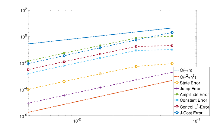
Figure 1: In the legend we see the following error rates: "State Error" stands for the $\|S_{\tau,h}(\bar{v}_{\tau,h},\bar{c}_{\tau,h})-S(\bar{v},\bar{c})\|$ error. The "Jump Error", "Amplitude Error", and "Constant Error" are the error rates we defined in Theorem 10. The line corresponding to "Control $L^{1}$-Error" is the $\|\bar{u}-\bar{u}_{\tau,h}\|_{L^{1}(I)}$ error and "J-Cost Error" stands for $|\tilde{J}(\bar{v},\bar{c})-\tilde{J}(\bar{v}_{\tau,h},\bar{c}_{\tau,h})|$. The discretization parameters are chosen as $\tau=2^{-k}$ and $h=2\cdot\sqrt{2}\cdot 2^{-k}$ with $k=4,5,\cdots,8$ and the grids are refined simultaneously.

In Figure 1 we observe that the error in state variable measured in the $L^{2}(\Omega_{T})$-norm, in the control variable measured in the $L^{1}(I)$-norm as well as in the cost functional converge like $O(\tau^{2}+h^{2})$. The same is true for the error in the jump positions $t_{j,1}$, the magnitudes of the jumps $c_{j}^{1}$ and the offset $c_{1}$. Thus the predicted error rates are verified.

References

- [1] L. Ambrosio, N. Fusco, and D. Pallara. Functions of bounded variation and free discontinuity problems. Oxford Mathematical Monographs, The Clarendon Press Oxford University Press, New York, 2000.
- [2] G. A. Anastassiou. Intelligent Computations: Abstract Fractional Calculus, Inequalities, Approximations. Studies in Computational Intelligence. Springer International Publishing, 2017.
- [3] K. Bredies and H. K. Pikkarainen. Inverse problems in spaces of measures. ESAIM Control Optim. Calc. Var., 19:190–218, Jan. 2013.
- [4] E. Casas, F. Kruse, and K. Kunisch. Optimal control of semilinear parabolic equations by bv-functions. SIAM J. Control Optim., 55(3), 1752–1788, 2017.
- [5] E. Casas and K. Kunisch. Optimal control of semilinear elliptic equations in measure spaces. SIAM Journal on Control and Optimization, 52(1):339–364, 2014.
- [6] E. Casas and K. Kunisch. Analysis of optimal control problems of semilinear elliptic equations by bv-functions. Set-Valued and Variational Anaylsis, 1-25, 2017.
- [7] E. Casas, K. Kunisch, and C. Pola. Some applications of BV functions in optimal control and calculus of variations. ESAIM: Proceedings, 4:181–198, 1998.
- [8] E. Casas, K. Kunisch, and C. Pola. Regularization by functions of bounded variation and applications to image enhancement. Appl. Math. and Optimization, 40:229–258, 1999.
- [9] E. Casas and F. Tröltzsch. A general theorem on error estimates with application to a quasilinear elliptic optimal control problem. Computational Optimization and Applications, 53(1):173–206, 2012.
- [10] C. Clason and K. Kunisch. A duality-based approach to elliptic control problems in non-reflexive Banach spaces. ESAIM Control Optim. Calc. Var., 17:243–266, 2011.
- [11] I. Ekeland and R. Témam. Convex Analysis and Variational Problems, Classics in Appl. Math. SIAM, Philadelphia, PA, english ed., 1999.
- [12] S. Engel and K. Kunisch. Optimal control of the linear wave equation by time-depending bv-controls: A semi-smooth newton approach. ArXiv manuscript e-prints, 2018.
- [13] D. Hafemeyer, F. Mannel, I. Neitzel, and B. Vexler. Finite element error estimates for one-dimensional elliptic optimal control by bv functions. ArXiv e-prints 1902.05893v2, and Math. Control Relat. Fields, accepted, 2019.
- [14] O. Ladyjenskaya. Boundary value problems of mathematical physics. Nauka, Moscow, 1973.
- [15] K. Pieper and B. Vexler. A priori error analysis for discretization of sparse elliptic optimal control problems in measure space. SIAM Journal on Control and Optimization 51(4),pp. 2788- 2808, 2013.
- [16] K. Pieper and D. Walter. Linear convergence of accelerated conditional gradient algorithms in spaces of measures. ArXiv e-prints 1904.09218v1, 2019.
- [17] P. Trautmann, B. Vexler, and A. Zlotnik. Finite element error analysis for measure-valued optimal control problems governed by a 1d wave equation with variable coefficients. Mathematical Control and Related Fields, 8:411, 2018.
- [18] P. Trautmann, B. Vexler, and A. A. Zlotnik. Finite element error analysis for measure-valued optimal control problems governed by a 1d wave equation with variable coefficients. Mathematical Control and Related Fields, 8(2), pp. 411-449, 2018.
- [19] A. A. Zlotnik. Convergence rate estimates of finite-element methods for second-order hyperbolic equations. numerical methods and applications, p.153 et.seq. Guri I. Marchuk, CRC Press, 1994.