Understanding Adversarial Robustness: The Trade-off between Minimum and Average Margin

Abstract.

Deep models, while being extremely versatile and accurate, are vulnerable to adversarial attacks: slight perturbations that are imperceptible to humans can completely flip the prediction of deep models. Many attack and defense mechanisms have been proposed, although a satisfying solution still largely remains elusive. In this work, we give strong evidence that during training, deep models maximize the minimum margin in order to achieve high accuracy, but at the same time decrease the average margin hence hurting robustness. Our empirical results highlight an intrinsic trade-off between accuracy and robustness for current deep model training. To further address this issue, we propose a new regularizer to explicitly promote average margin, and we verify through extensive experiments that it does lead to better robustness. Our regularized objective remains Fisher-consistent, hence asymptotically can still recover the Bayes optimal classifier.

1. Introduction

Traditionally, training more accurate classifiers has been much of the focus of machine learning research. More recently, as machine learning models start to penetrate into safety-critical applications, their robustness against random or even adversarial manipulations has drawn a lot of attention. The work of Szegedy et al. [1] demonstrated surprisingly that it is possible to craft very minimal changes to an input image that (a) is clearly not perceivable by humans but (b) can completely flip the predictions of state-of-the-art deep models. Such detrimental perturbations are called adversarial examples and have raised serious concerns on the safety of deep models.

Since the work of Szegedy et al. [1], a sequence of works have proposed new attack algorithms to generate adversarial examples [e.g. 2, 3, 4, 5, 6, 7, 8, 9], as well as defensive techniques [e.g. 10, 11, 12, 13, 14] to train more robust models. There even appears to be an arm race between attack and defense techniques: new defense techniques are shown nonrobust under stronger attacks shortly after being proposed [15]. Thus, a line of research focusing on provable certification of (non)robustness has emerged. For example, one can use the Lipschitz constant of the network to provide a lower bound on the amount of needed adversarial perturbations [e.g. 16, 17, 18, 19]. More recently, certification methods base on mixed integer programming (MIP) [20, 21] have been proposed to provide more accurate lower bounds. However, due to the NP-hardness of MIP, convex relaxations [22, 23, 24, 25, 26, 27] have been popular for scaling these provable certification methods to larger models.

In this paper, we study adversarial robustness from a margin perspective. The notion of margin distribution dates back to [28, 29, 30, 31], which provide generalization bounds based on the margin distribution. Later on, algorithms that control margin distribution for better generalization performance have been proposed [32]. In this work, however, we connect the notion of margin with adversarial robustness, and we reveal a surprising trade-off between minimum and average margin in standard deep model training. In particular, the recent result in [33] implies that on a linearly separable dataset a linear classifier trained with (stochastic) gradient descent converges to the SVM solution, under mild conditions on the loss function. Since SVM explicitly maximizes the minimum margin, any linear classifier would eventually achieve the same. However, our experiments reveal that the average margin is greatly reduced during training. In other words, models maximize the minimum margin at the expense of reducing the average margin hence becoming more susceptible to adversarial attacks. This surprising phenomenon was also confirmed on linearly nonseparable datasets and a variety of nonlinear classifiers. Interestingly, a few defense methods based on margin maximization have been proposed [34, 35, 36], which through our work, should be understood as maximizing the average margin, as opposed to the minimum margin.

To overcome the trade-off between minimum margin and average margin in standard training, we propose the standard training objective with an average-margin promoting regularizer. We prove that the regularized objective remains Fisher consistent, if the original loss is so. This means as sample size grows, the classifier obtained through optimizing our regularized objective still approaches the Bayes optimal classifier, while potentially is much more robust than standard training. Our regularizer can be easily extended to multiclass and nonlinear classifiers. We confirm the latter point through extensive experiments on two standard datasets and a variety of different models and settings.

To summarize, we make the following contributions in this work:

• We reveal the intrinsic trade-off between minimum margin and average margin;

• We propose a new regularizer that explicitly promotes average margin and retains Fisher consistency;

• We perform extensive experiments to confirm the effectiveness of our new regularizer.

2. Background

We consider the multi-category classification problem. Given a set of $n$ training instances $\{(\mathbf{x}_{i},y_{i})\in\mathcal{X}\times[c]:i=1,\ldots,n\}$, where the feature domain $\mathcal{X}\subseteq\mathds{R}^{d}$ and $[c]:=\{1,\ldots,c\}$ with $c\geq 2$ the number of categories, we are interested in finding a classifier $h:\mathcal{X}\to[c]$, or equivalently, a set partition $\mathsf{F}_{1},\ldots,\mathsf{F}_{c}$ of the domain $\mathcal{X}$ such that $\cup_{k}\mathsf{F}_{k}=\mathcal{X}$ and for all $k\neq l$, $\mathsf{F}_{k}\cap\mathsf{F}_{l}=\emptyset$. Often in practice, the classifier $h$ is learned through a vector-valued function $\mathbf{f}:\mathcal{X}\to\mathds{R}^{c}$, with the argmax prediction rule employed to predict the label $\hat{y}$ of a test sample $\mathbf{x}$ as follows:

(1) $$\hat{y}=\hat{y}(\mathbf{x}):=\arg\max_{k=1,\ldots,c}f_{k}(\mathbf{x}),\qquad f_{k}:\mathcal{X}\to\mathds{R},\qquad\mathbf{f}=(f_{1},\ldots,f_{c}).$$

As is well-known, the two representations of a classifier, i.e. either through a set partition $\{\mathsf{F}_{k}\}$ or through a vector-valued function $\mathbf{f}$, are equivalent. We will use both representations interchangeably.

In their seminal work, Szegedy et al. [1] defined the robustness of a classifier $\mathbf{f}$ on a test sample $\mathbf{x}$ as the minimum perturbation needed to flip its prediction (c.f. (1)):

(2) $$\mathsf{r}(\mathbf{x})=\inf\{\|\mathbf{z}\|:\mathbf{x}+\mathbf{z}\in\mathcal{X},~{}\hat{y}(\mathbf{x}+\mathbf{z})\neq\hat{y}(\mathbf{x})\},$$

where $\|\cdot\|$ is an abstract norm (e.g. the familiar $\ell_{p}$ norm) for measuring the amount of perturbation. This notion of robustness turns out to have a very intuitive geometric meaning, as we detail below. We remind that we also represent a classifier $\mathbf{f}$ as a set partition $\{\mathsf{F}_{1},\ldots,\mathsf{F}_{c}\}$.

For any $\mathbf{x}\in\mathcal{X}$, define $\hat{y}(\mathbf{x})\in[c]$ so that $\mathbf{x}\in\mathsf{F}_{\hat{y}(\mathbf{x})}$, i.e. $\hat{y}(\mathbf{x})$ is the predicted label of our classifer. We define the distance from a point $\mathbf{x}\in\mathcal{X}$ to a set $\mathsf{F}\subseteq\mathcal{X}$ as:

(3) $$\mathsf{d}(\mathbf{x},\mathsf{F}):=\inf\{\|\mathbf{x}-\mathbf{z}\|:\mathbf{z}\in\mathsf{F}\}.$$

Recall that the notations $\mathop{\mathrm{cl}}\mathsf{F}$, $\mathop{\mathrm{int}}\mathsf{F}$, $\bar{\mathsf{F}}$ and $\mathop{\mathrm{bd}}\mathsf{F}$ denote the closure, interior, complement and the boundary of a point set $\mathsf{F}$, respectively. We remark that for any set $\mathsf{F}$:

(4) $$\mathsf{d}(\mathbf{x},\mathsf{F})=\begin{cases}0,&~{}\mbox{ if }\mathbf{x}\in\mathop{\mathrm{cl}}\mathsf{F}\\ \mathsf{d}(\mathbf{x},\mathop{\mathrm{bd}}\mathsf{F}),&~{}\mbox{ otherwise }\end{cases},$$

which will be important when we aim to optimize some function of the distance.

Note that $\mathsf{d}(\mathbf{x},\mathsf{F}_{\hat{y}})$ is the distance to the decision boundary, which captures the definition (2) exactly:

Proposition 1.

Let $\mathbf{f}:\mathcal{X}\to\mathds{R}^{c}$ be a vector-valued function that, if augmented with the argmax prediction rule (1), leads to the following sets (classifier): for all $k\in[c]$,

(5) $$\mathsf{F}_{k}:=\{\mathbf{x}\in\mathcal{X}:f_{k}(\mathbf{x})=\max_{l=1,\ldots,c}f_{l}(\mathbf{x})\},$$

where we break ties arbitrarily. Then the robustness definition in Equation 2 equals to $\mathsf{d}(\mathbf{x},\mathsf{F}_{\hat{y}})$.

We are now ready to define the individual margin of a sample pair $(\mathbf{x},y)$ w.r.t. the classifier $\{\mathsf{F}_{k}\}$ as:

(6) $$\mathsf{m}(\mathbf{x},y):=\mathsf{m}(\mathbf{x},y;\{\mathsf{F}_{k}\}):=\mathop{\mathrm{sign}}(\hat{y}(\mathbf{x}),y)\cdot\mathsf{d}(\mathbf{x},\mathop{\mathrm{bd}}\mathsf{F}_{\hat{y}}),$$

where we define $\mathop{\mathrm{sign}}(\hat{y},y)=1$ if $\hat{y}=y$ and $\mathop{\mathrm{sign}}(\hat{y},y)=-1$ otherwise. Namely, when predicting correctly, $\mathsf{m}(\mathbf{x},y)$ is the distance to the decision boundary, i.e. the minimum perturbation needed to change the prediction; whereas when predicting wrongly, it is the negation of the distance to the decision boundary, i.e. the minimum perturbation needed to correct the prediction. We then define

• minimum margin: $\min_{1\leq i\leq n}\mathsf{m}(\mathbf{x}_{i},y_{i})$

• average margin: $\frac{1}{n}\sum_{i=1}^{n}|\mathsf{m}(\mathbf{x}_{i},y_{i})|$, simply the average distance to the decision boundary.

Although the definition (3) applies for any norm, we will focus on $l_{2}$ margin later, as some current results of implicit minimum margin maximization [33, 37, 38] only holds for $l_{2}$ norm, which will be discussed in §3. From now on, we use $\|\cdot\|$ to denote the Euclidean norm.

3. Minimum vs. Average Margin: A Case Study

In this section, we study a simple example to demonstrate the trade-off between minimum and average margin. In statistical learning theory, it is well-known that we can bound the generalization error of a classifier using empirical margins [39]. In particular, the celebrated support vector machines (SVM) explicitly maximize the minimum margin (on any linearly separable dataset). In adversarial learning, however, we argue that average margin is more indicative of the robustness of a classifier.

Our main observations in this section are: (a) Current machine learning models, especially when they become deep and powerful, implicitly maximize the minimum margin to achieve high accuracy; (b) there appears to be an inherent trade-off between minimum margin and average margin. In particular, by maximizing the minimum margin, the model also (unconsciously) minimizes the average margin, hence becomes susceptible to adversarial attacks. Note that we do not claim minimum margin always contradicts average margin. It does not, as can be easily shown through carefully constructed toy datasets (e.g. a hightly symmetric dataset). Our empirical observation is that there does appear to be some tension between the two notions of margin on real datasets.

To begin with, we first demonstrate that minimum margin is maximized during standard training. In fact, this can be formally established through the implicit bias of optimization algorithms, such as (stochastic) gradient descent which is ubiquitously used in training deep models. Recall that on a (linearly) separable dataset, (hard-margin) linear SVM explicitly maximizes the minimum margin. The following result, due to Soudry et al. [33], confirms the same for most models currently used in machine learning, including logistic regression.

Theorem 1 ([33]).

For almost all linearly separable binary datasets and any smooth decreasing loss with an exponential tail, gradient descent with small constant step size and any starting point $\mathbf{w}_{0}$ converges to the (unique) solution $\widehat{\mathbf{w}}$ of hard-margin SVM, i.e. $\lim_{t\to\infty}\frac{\mathbf{w}_{t}}{\left\|\mathbf{w}_{t}\right\|}=\frac{\widehat{\mathbf{w}}}{\left\|\widehat{\mathbf{w}}\right\|}.$

Note that the margin of a linear classifier $f(\mathbf{x})=\mathbf{w}^{\top}\mathbf{x}$, with decision boundary $\mathop{\mathrm{bd}}\mathsf{F}:=\{\mathbf{x}:\mathbf{w}^{\top}\mathbf{x}=0\}$, can be computed in closed-form: $\mathsf{d}(\mathbf{x},\mathop{\mathrm{bd}}\mathsf{F})=\tfrac{|\mathbf{w}^{\top}\mathbf{x}|}{\|\mathbf{w}\|}$, which only depends on the direction of the weight vector $\mathbf{w}$. Thus, Theorem 1 implies in particular that if we optimize logistic regression by gradient descent on a linearly separable dataset, then we implicitly maximize the minimum margin, just as in SVM. Besides linear classifiers, the same implicit bias towards maximizing the minimum margin has also been discovered for deep networks [37, 38].

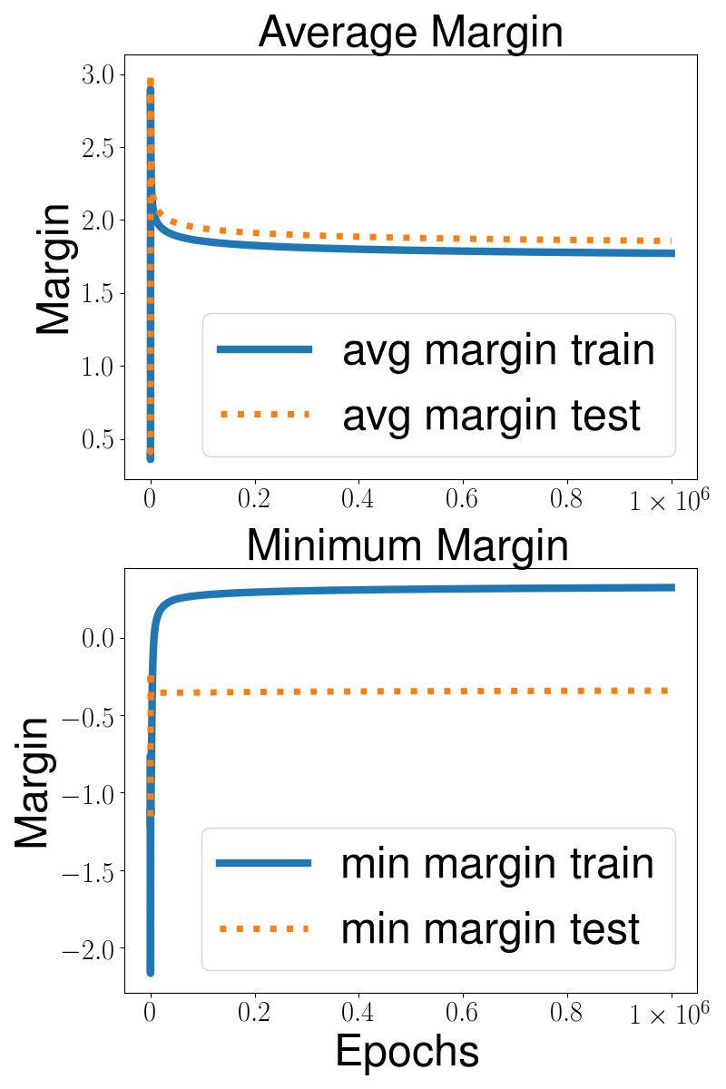
(a) Margins during training of LR.
Upper: Average margin on training and test set.
Lower: Minimum margin on training and test set.

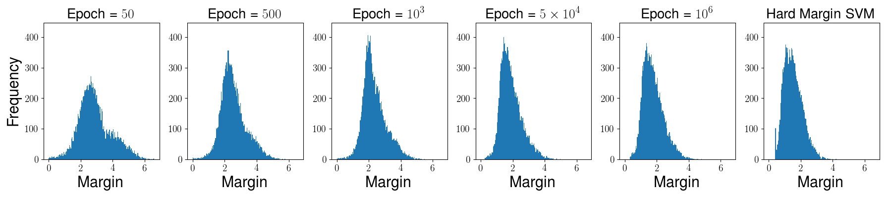
(b) Margin histograms on the training set. First 5 plots: Margin histograms of LR during training. Last plot: Margin histogram of SVM, which LR margins converge to. During training, the histogram continues shifting towards left.

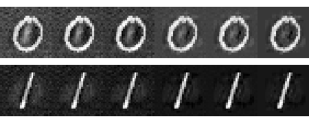
(c) Visualization of adversarial examples at different epochs during training. First row: adversarial examples for $0$. Second row: adversarial examples for $1$. Adversarial examples in the same column are generated in the same epoch. Adversarial examples gradually become imperceptible. Zoom the figure for better visualization.

It is then natural to ask the next question: How does average margin change during training? To answer this question, we train a binary logistic regression (LR) using gradient descent on MNIST to discriminate $0$’s from $1$’s. Note that the subset of MNIST consisting of only $0$’s and $1$’s is indeed linearly separable, as LR achieves zero training error (see Figure 4 in appendix). All conditions of Theorem 1 are thus satisfied, and we expect LR to maximize minimum margin. Indeed, Figure 1(a) confirms that the minimum margin continues to increase during training until it approaches that of hard-margin SVM, as predicted by Theorem 1. Meanwhile, the average margin decreases drastically after a few epochs at the very beginning, and then keeps decreasing. Interestingly, the minimum margin continues to increase while the average margin continues to decrease even after the training error reaches zero, which means the decision boundary still changes even after training error diminishes.

To gain further insight, in Figure 1(b) we plot the histogram of margins at different training epochs. We observe that the margin distribution shifts towards the left during training and eventually approaches that of hard-margin SVM. In other words, during training the majority of data is pushed towards the decision boundary, leading LR to become more and more vulnerable to adversarial attacks. Indeed, Figure 1(c) confirms this by visualizing the adversarial examples constructed at different training epochs. Note that for a linear classifier the adversarial example with minimum perturbation can be explicitly determined as

(7) $$\textstyle\mathbf{x}^{adv}=\mathbf{x}-\frac{\mathbf{w}^{\top}\mathbf{x}}{\|\mathbf{w}\|^{2}}\mathbf{w},$$

which is the point on the decision boundary that is closest to the training example $\mathbf{x}$. As shown in Figure 1(c), the adversarial examples gradually become more and more imperceptible, indicating that LR becomes more and more vulnerable to adversarial attacks.

A few remarks are in order. First, we have carefully designed our experiment so that (a) the theoretical results in Theorem 1 apply; (b) the margins and adversarial examples can be explicitly computed. However, similar phenomenon is also observed for deep models on different datasets where the conditions of Theorem 1 may be violated or the margins can only be approximately computed; see §5 for more of these experiments. Second, we remark that the decrease of average margin cannot be caused by overfitting. This is because the test accuracy continues to decrease during training (see training curves in Figure 4 of the appendix). Moreover, we observe that the average margin decreases on both training and test sets. To summarize, we conclude that practically, deep models try to maximize the minimum margin during training at the expense of sacrificing the average margin, hence become susceptible to adversarial attacks. To address this issue, in the next section we propose to explicitly optimize the average margin through appropriate regularization.

4. An Average Margin Regularizer

In this section, we propose a regularization function to explicitly promote average margin. We first handle linear classifiers in §4.1 through maximizing the average margin in the input space directly. For nonlinear classifiers, maximizing the margin in the input space directly is intractable. Instead, we maximize a lower bound of input space margins in §4.2, through simultaneously maximizing feature space margin and controlling the Lipschitz constant of the network.

The most straightforward way to improve robustness of a classifier is through explicit regularization. In particular, we consider the following regularized problem:

(8) $$\min_{\mathbf{f}:\mathcal{X}\to\mathds{R}^{c}}~{}\frac{1}{n}\sum_{i=1}^{n}\phi(y_{i},\mathbf{f}(\mathbf{x}_{i}))-\lambda\cdot\frac{1}{n}\sum_{i=1}^{n}\mathbf{1}_{y_{i}=\hat{y}_{i}}\cdot\mathsf{d}_{\tau}(\mathbf{x}_{i},\mathop{\mathrm{bd}}\mathsf{F}_{y_{i}})$$

where $\phi$ is the loss function we use to measure the accuracy of our classifier $\mathbf{f}$, $\{\mathsf{F}_{k}\}$ are the sets induced by $f$ (using the argmax rule) , $\lambda\geq 0$ is the regularization constant that balances the two objectives, and $\mathsf{d}_{\tau}=\min\{\tau,\mathsf{d}\}$ is the truncated distance. In particular, we only maximize the margin when the classifier makes a correct prediction and the margin is capped at $\tau$ to avoid being dominated by some outliers. We show next how to solve (8) when $\mathbf{f}$ is a binary linear classifier.

4.1. Binary Linear Classifier

In this section we assume there are two classes, i.e. $c=2$ and we consider the linear classifier $f(\mathbf{x})=\mathbf{w}^{\top}\mathbf{x}$ (w.l.o.g. we omit the bias term). Correspondingly, let $\mathsf{F}_{+}=\{\mathbf{x}\in\mathcal{X}:\mathbf{w}^{\top}\mathbf{x}\geq 0\}$ and the distance $\mathsf{d}(\mathbf{x},\mathop{\mathrm{bd}}\mathsf{F}_{+})=\tfrac{|\mathbf{w}^{\top}\mathbf{x}|}{\|\mathbf{w}\|}.$ The regularized problem (8) reduces to

(9) $$\min_{\left\|\mathbf{w}\right\|=1}~{}~{}\sum_{i=1}^{n}\phi(y_{i}\mathbf{w}^{\top}\mathbf{x}_{i})-\lambda\cdot\sum_{i=1}^{n}[y_{i}\mathbf{w}^{\top}\mathbf{x}_{i}]_{0}^{\tau},$$

where $[t]_{0}^{\tau}=\min(\max(t,0),\tau)$. The second regularization term can be written as a difference of two convex functions. Indeed, define $H_{s}(x)=\max(0,s-x)$, then

(10) $$-[t]_{0}^{\tau}=H_{\tau}(t)-H_{0}(t)+\tau,$$

and the objective function simplifies to

(11) $$\min_{\left\|\mathbf{w}\right\|=1}~{}~{}\sum_{i=1}^{n}\phi(y_{i}\mathbf{w}^{\top}\mathbf{x}_{i})+\lambda\cdot\sum_{i=1}^{n}[H_{\tau}-H_{0}](y_{i}\mathbf{w}^{\top}\mathbf{x}_{i}),$$

where $\lambda\geq 0$ and $\tau\geq 0$ are tuning hyperparameters.

Quite pleasantly, our average margin regularizer not only promotes robustness, it also retains Fisher consistency (aka classification-calibrated), namely that the classifier we obtain by minimizing the regularized objective in (9) still approaches the Bayes optimal classifier, as sample size $n$ increases to infinity.

Definition 1 (Fisher consistency [40]).

Suppose $\phi:\mathds{R}\to\mathds{R}$ is a loss function and $\eta\in\left[0,1\right]$. For any $\alpha\in\mathbb{R}$, define the conditional $\phi$-risk as $C_{\eta}^{\phi}(\alpha)=\eta\phi(\alpha)+(1-\eta)\phi(1-\alpha).$ We say a loss $\phi$ is Fisher consistent if for any $\eta\neq\frac{1}{2}$,

(12) $$\inf_{\alpha:\alpha(2\eta-1)\leq 0}C_{\eta}^{\phi}(\alpha)>\inf_{\alpha\in\mathds{R}}C_{\eta}^{\phi}(\alpha).$$

For a Fischer consistent loss functions $\phi$, (12) implies that to minimize the $\phi$-risk, $\alpha$ should satisfy $\alpha(2\eta-1)>0$, i.e. the decision $\alpha$ of our classifier should match the decision $\mathop{\mathrm{sign}}(2\eta-1)$ of the Bayes classifier (which is optimal under the 0-1 loss). Fisher-consistency is a necessary condition for any reasonable loss, if our goal is to approximate the Bayes optimal classifier. The following result confirms the Fisher-consistency of our regularized objective (9) (see the proof in appendix).

Theorem 2.

Suppose the loss function $\phi$ is decreasing, continuous, bounded below and $\phi^{\prime}(0)<0$. Let $\psi=H_{\tau}-H_{0}$ be our average margin regularizer. Then the regularized loss $\ell=\phi+\lambda\psi$ is Fisher consistent for any $\lambda,\tau\geq 0$.

The above condition on the loss $\phi$ is reasonable: it basically guarantees $\phi$ itself to be Fisher consistent. Common loss functions, such as the logistic loss, exponential loss and hinge loss, all satisfy this condition. Thus, our average margin regularizer, when combined with these typical, Fisher consistent loss functions, remains Fisher consistent.

4.2. Extension to Multiclass Deep Models

For deep neural networks, even computing the margin in the input space is already NP-hard [41, 19], let alone optimizing it. However, the margin in the feature space provides a lower bound of the margin in the input space. For example, let $\mathbf{f}$ be a deep neural network with $L$ layers, $\mathbf{f}(\mathbf{x})=W_{L}\cdot\sigma(W_{L-1}\cdot\sigma(\cdots\sigma(W_{1}\cdot\mathbf{x})))$, where $\sigma$ is the activation function. Let $\Phi(\mathbf{x})$ be the output of the second last fully connected layer, i.e. $\Phi(\mathbf{x})=\sigma(W_{L-1}\cdot\sigma(\cdots\sigma(W_{1}\cdot\mathbf{x})))$, then

(13) $$\left\|\Phi(\mathbf{x}_{1})-\Phi(\mathbf{x}_{2})\right\|\leq Lip(\Phi)\left\|\mathbf{x}_{1}-\mathbf{x}_{2}\right\|,$$

where $Lip(\Phi)$ is the Lipschitz constant of the feature map $\Phi$. The tightness of this bound is determined by the Lipschitz constant of the model. For example, if the model is $1$-Lipschitz with $Lip(\phi)=1$, then the margin in the input space $\mathcal{X}$ is exactly lower bounded by the margin in the feature space $\left\{\Phi(\mathbf{x}):\mathbf{x}\in\mathcal{X}\right\}$. The bound (13) motivates a natural way to optimize the margin in input space: we simultaneously fix the Lipschitz constant and maximize the margin in feature space. Note that this perspective allows us to treat any deep network as first performing a nonlinear feature transform through $\Phi$, and then applying a linear classifier on top.

The Lipschitz constant can be bounded by the product of norms of the weight matrices $\prod_{i}\left\|W_{i}\right\|_{2}$, where $W_{i}$ is the weight matrix in layer $i$, assuming the activation function is 1-Lipschitz, for instance ReLU [1]. To control the overall Lipschitz constant $Lip(\Phi)$, ideally, we want to enforce the Lipschitz constant of each layer to be exactly $1$, namely constraining the spectral norm of each weight matrix $W_{i}$ to be approximately 1. Inspired by [11, 42], we add an orthogonal penalty $\beta\left\|W_{i}W_{i}^{\top}-I\right\|_{\mathrm{F}}^{2},$ into our training objective, which encourages the weight matrices to be orthogonal hence having spectral norm close to $1$. For convolutional layers, we first flatten the convolutional filter and then apply the above penalty.

Once the Lipschitz constant is bounded, we directly maximize the average margin in the feature space, as a computationally efficient lower bound for promoting the average margin in the input space. Since our classifier is linear in the feature space, the distance to the decision boundary can be computed as in §4.1:

(14) $$\mathsf{d}(\mathbf{x},\mathop{\mathrm{bd}}\mathsf{F}_{\hat{y}})=\min_{k\neq\hat{y}}(\mathbf{w}_{\hat{y}}-\mathbf{w}_{k})^{\top}\Phi(\mathbf{x}),$$

where $\mathbf{w}_{k}$ is the (normalized) weight vector in the final layer for the $k$-th class. Similar to the binary case, we only maximize the margin for correctly classified examples and truncate the margin if it exceeds the threshold $\tau$. In the end, our regularized objective is,

(15) $$\sum_{i=1}^{n}\phi\left(y_{i},\mathbf{f}(\mathbf{x}_{i})\right)-\lambda\left[\min_{k\neq y_{i}}(\mathbf{w}_{y_{i}}-\mathbf{w}_{k})^{\top}\Phi(\mathbf{x}_{i})\right]_{0}^{\tau}+\beta\sum_{1\leq l\leq L}\|W_{l}W_{l}^{\top}-I\|_{\mathrm{F}}^{2},$$

where the first term is the standard training loss (such as cross-entropy), the third term is the orthogonal constraint for controlling the Lipschitz constant of the network, and the second term is the average margin penalty in the feature space, which also maximizes the input space average margin, provided that the Lipschitz constant of the network is indeed close to unity.

5. Experiments

In this section, we conduct experiments to (a) verify the minimum-average margin trade-off on a variety of (nonlinear) deep models; (b) demonstrate the effectiveness of our average margin regularizer. First, we train six models with various architectures on MNIST and CIFAR10 to verify the trade-off again. Then, we retrain these models with our average margin regularizer, and confirm that our regularizer indeed can effectively promote the average margin. Finally, we compare our average margin regularizer with other state-of-the-art defense techniques in the literature and find that our regularizer achieves comparable performance in terms of robustness and accuracy.

5.1. Approximating Distance

In general, exactly computing the distance to the decision boundary of deep models is intractable [41, 19]. Instead, we use the following Lipschitz lower bound as a reasonable approximation:

Theorem 3 ([16]).

Suppose $\mathbf{f}:\mathds{R}^{d}\to\mathds{R}^{c}$ is a multiclass classifier (with argmax prediction rule). Then, for any $r>0$:

(16) $$\mathsf{d}(\mathbf{x},\mathop{\mathrm{bd}}\mathsf{F}_{\hat{y}})\geq\min\left\{\min_{k\neq\hat{y}}\tfrac{f_{\hat{y}}(\mathbf{x})-f_{k}(\mathbf{x})}{L^{k}_{\mathbf{x}}},r\right\},$$

where $L^{k}_{\mathbf{x}}$ is the local Lipschitz constant of $f_{\hat{y}}(\mathbf{x})-f_{k}(\mathbf{x})$ over the ball $B(\mathbf{x},r)$

The lower bound (16) is in fact exact when $\mathbf{f}$ is linear, and for general nonlinear $\mathbf{f}$, it is reasonably close to the true distance, as shown empirically in [17]. Here, our estimate for the Lipschitz constant $L^{k}_{\mathbf{x}}$ is simply the maximum norm of the gradient (difference) of many random samples in the ball $B(\mathbf{x},r)$, as we found this simple strategy is reasonably efficient and accurate. For space limits, we defer the experimental details on approximating this distance to the appendix.

5.2. Verifying the Margin Trade-off again on Deep Nonlinear Models

Due to space limits, here we only present the experimental results on the CIFAR10 dataset, while results on MNIST can be found in the appendix. For each model, we plot the average margin and minimum margin w.r.t. the number of training epochs in Figure 2. It is clear that similar phenomenon as those in §3 can be observed: the minimum margin continues increasing while at the same time the average margin keeps decreasing. This again highlights an intrinsic trade-off between minimum margin and average margin. In addition, we consistently observed that the average margin continues to decrease even after the training/test error has saturated (see training curves Figure 5 in the appendix).

To investigate how the margin distribution changes during training, we plot the histograms of margins in Figure 8 (appendix). As training proceeds, we observe again the margin distribution shifts towards left, meaning the majority of data points is pushed closer to the boundary. To some extent, this provides compelling explanation of the non-robustness of deep models: although achieving high accuracy by maximizing the minimum margin, the average margin, which is a better indicator of robustness, is at serious jeopardy. Note that early stopping, while helps preventing the average margin to decrease unnecessarily, is not sufficient by itself to promote average margin. Instead, an explicit average margin regularizer is more effective, as we show next.

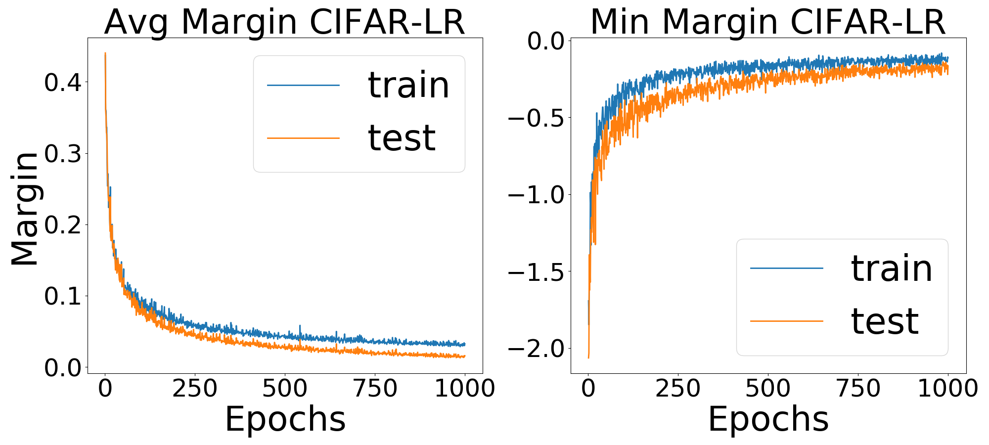
Avg vs Min CIFAR-LR

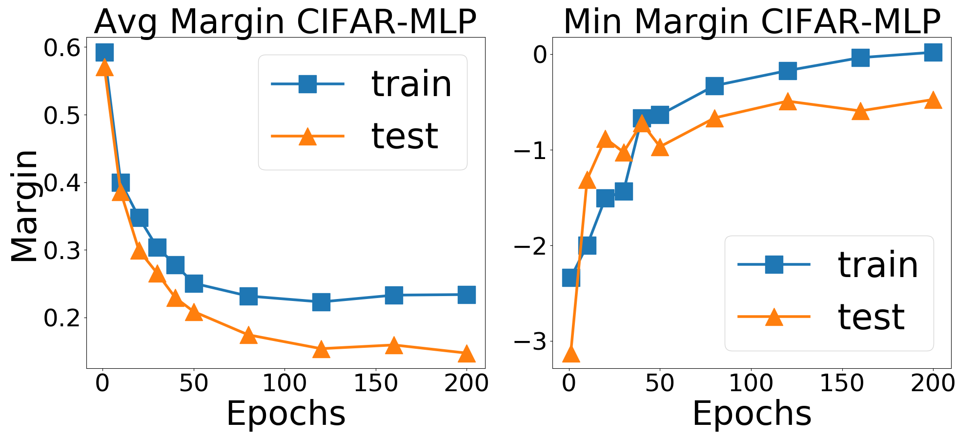
Avg vs Min CIFAR-MLP

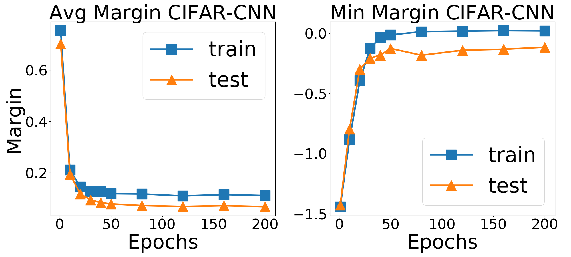
Avg vs Min CIFAR-CNN

Figure 2. Average and minimum margin during training of different models on CIFAR10.

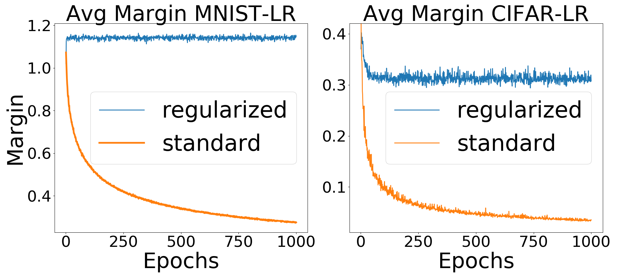
Avg Margin of LR

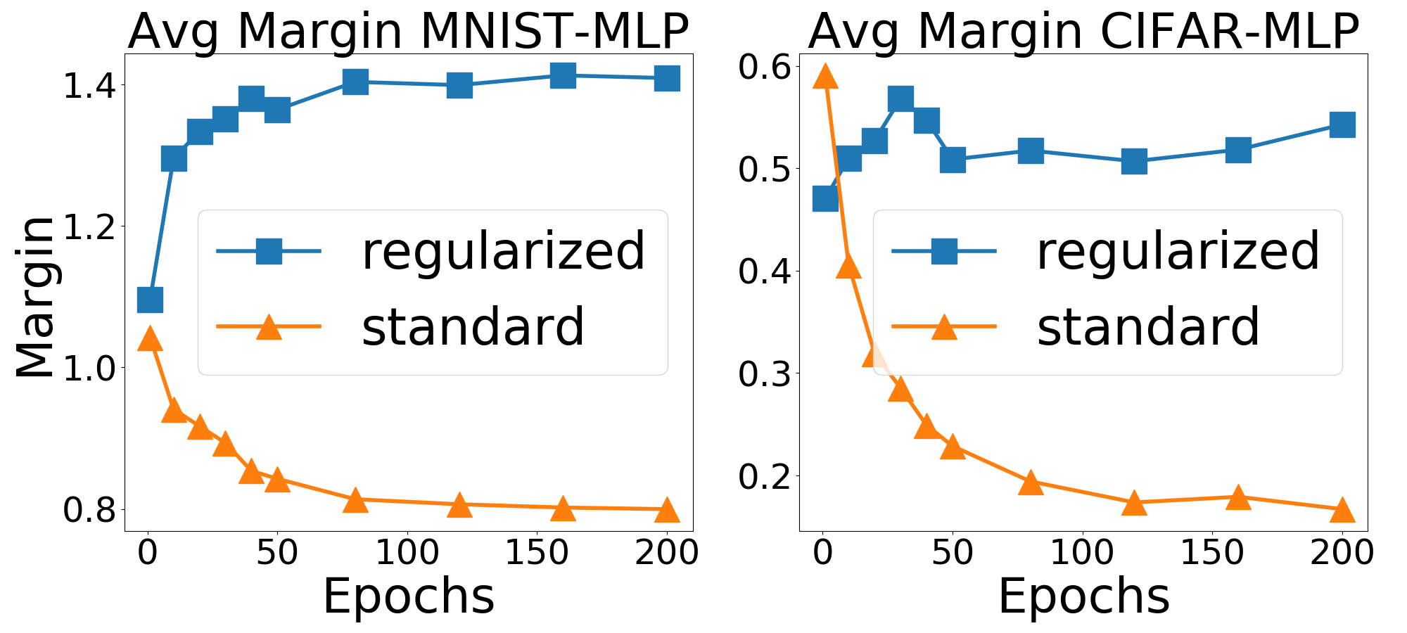
Avg Margin of MLP

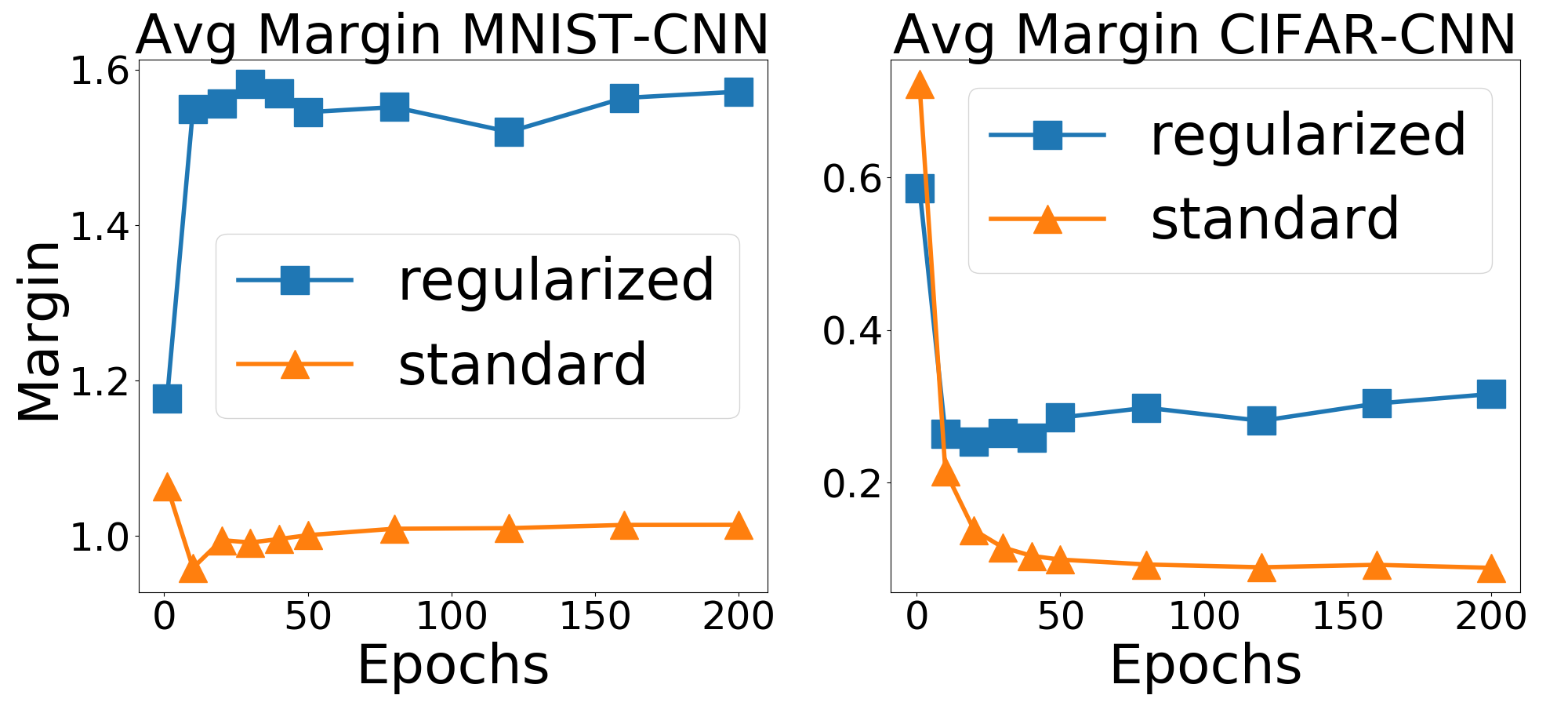
Avg Margin of CNN

Figure 3. Average margin of regularized and standard training.

5.3. Average Margin Regularizer

We retrain six models augmented with our average margin regularizer, and compare the average margin with standard training in Figure 3. It is clear that with our average margin regularizer, the regularized models no longer sacrifice the average margin during training. For all six models, adding the average margin regularizer significantly improves adversarial robustness. For example, the average margin of LR and MLP become $2\sim 3$ times more than those of models with standard training. For CNN, the average margin is increased by a factor of $1.5\sim 2$.

Next, we compare our regularizer with Lipschitz constant regularization. In our regularizer, we use the orthogonal constraint $\|WW^{\top}-I\|_{\mathrm{F}}^{2}$ to control the Lipschitz constant. The idea of using orthogonal constraint as Lipschitz constant regularizer has been proposed before (e.g. Paserval networks [11] and defensive quantization [42]). Here, we prvide a comparison between Lipschitz constant regularization and our average margin regularizer. We evaluate models using clean accuracy, robust accuracy under $l_{2}$ norm projected gradient descent (PGD) attack [2], and the average margin. We run $1000$ iterations of PGD to generate adversarial examples, whose success serves as a good approximation of robust accuracy. The results can be found in Table 1. As we can see, when $\epsilon$, the amount of allowed perturbations, is small, the accuracy of our average margin regularizer is comparable to that of the Lipschitz constant regularizer (LCR); but as $\epsilon$ becomes larger, the average margin regularizer consistently outperforms the latter. Interestingly, LCR alone can also improve adversarial robustness marginally [11, 42], when $\epsilon$ is small. This may be caused by implicit max-margin effect of the loss function used in training. However, as $\epsilon$ becomes larger, the robust accuracy of LCR is inferior to our method, sometimes even worse than standard training, which is also confirmed in the experimental results in [11, 36]. This implies that controlling Lipschitz constant alone may not be enough to train a robust model. Instead, one needs to maximize the average margin explicitly.

We also compare our method with deep defense (DD) [36], PGD adversarial training (Adv) [12] and the maximum margin regularizer (MMR) [35], which maximizes the linear region of ReLU netowrks. The results are shown in Table 2. Compared with standard training, our method can significantly improve model robustness. On MNIST, our method achieves overall better robust accuracy. On CIFAR10, our method achieves comparable results as adversarial training and deep defense. In addition, our method consistently outperforms MMR on both datasets. Moreover, our method is more efficient than adversarial training and deep defense. In fact, adversarial training would increase the training time by the number of PGD iterations (typically tens or hundreds), and deep defense is even more time consuming, to a point where it can only be applied as fine-tuning [36], while the training time of our method is roughly the same as the standard training.

Table 1. Comparision between AMR (our average margin regularizer) and LCR (Lipschitz constant regularization). Column 4-9: clean accuracy. Column 5-8: robust accuracy under $l_{2}$ PGD attack. The last column: average margin.

	Models	Method	Clean	$\epsilon=0.5$	$\epsilon=1.0$	$\epsilon=1.5$	$\epsilon=2.0$	Avg Margin
MNIST	MLP	Std	98.24	89.26	49.23	15.78	5.06	0.80
		LCR	95.99	91.12	80.62	60.56	34.07	1.36
		AMR	96.01	91.18	81.01	62.93	38.44	1.41
	CNN	Std	99.14	95.95	90.48	88.72	87.52	1.01
		LCR	99.29	97.21	87.83	58.30	26.96	1.34
		AMR	99.25	97.90	97.60	97.51	97.33	1.40
	Models	Method	Clean	$\epsilon=0.1$	$\epsilon=0.2$	$\epsilon=0.3$	$\epsilon=0.4$	Avg Margin
CIFAR	MLP	Std	54.04	39.77	26.67	16.77	9.95	0.17
		LCR	50.09	46.23	41.65	37.09	32.62	0.45
		AMR	50.36	46.28	42.81	39.06	35.67	0.54
	CNN	Std	78.77	54.32	39.81	37.14	36.27	0.09
		LCR	80.54	70.84	58.72	44.82	32.54	0.26
		AMR	78.12	69.59	59.84	49.02	38.65	0.31

Table 2. Comparison between 5 different training methods: Std (standard training), DD (deep defense [36]), Adv (PGD adversarial training [12]), MMR (maximum margin regularizer [35]), and AMR (ours). Column 4: clean accuracy. Column 5-8: robust accuracy under $l_{2}$ PGD attack.

		Method	Clean	$\epsilon=0.5$	$\epsilon=1.0$	$\epsilon=1.5$	$\epsilon=2.0$
MNIST	LeNet	Std	98.98	95.75	80.59	44.36	22.64
		DD	99.34	97.64	92.09	83.53	79.35
		Adv	99.48	97.45	91.99	88.88	87.51
		AMR	99.01	96.80	94.03	93.61	93.12
	LeNetSmall	MMR	97.43	89.90	58.86	23.95	6.80
		AMR	97.83	91.94	73.70	32.56	8.79
		Method	Clean	$\epsilon=0.1$	$\epsilon=0.2$	$\epsilon=0.3$	$\epsilon=0.4$
CIFAR	ConvNet	Std	76.61	56.47	37.37	30.17	28.89
		DD	79.10	68.95	59.51	56.84	56.38
		Adv	75.27	68.79	61.79	54.35	47.00
		AMR	76.77	68.00	57.87	52.38	50.03
	LeNetSmall	MMR	59.07	49.01	39.42	30.41	22.53
		AMR	68.40	61.33	53.84	46.03	39.05

6. Conclusion

In this work, we studied adversarial robustness from a margin perspective. We discovered the intrinsic trade-off between minimum and average margin, which appears across different models and datasets. We gave strong empirical evidence that deep models maximize the minimum margin during training to achieve high accuracy, but at the expense of decreasing the average margin significantly hence becoming more susceptible to adversarial attacks. To address the issue, we designed a new regularizer to explicitly maximize average margin and to retain Fisher consistency. Our extensive experiments confirmed the effectiveness of our regularizer. In the future, we will theoretically analyze the trade-off to provide further insights to the phenomenon. Moreover, we plan to go beyond just maximizing average margin, by controlling other margin distribution statistics such as variance.

Appendix A Proofs

Proof of Proposition 1.

Indeed, according to the definitions in (5) and (2) we have

(17) $$\mathsf{r}(\mathbf{x}) =\inf\{\|\mathbf{z}\|:\mathbf{x}+\mathbf{z}\not\in\mathsf{F}_{\hat{y}(\mathbf{x})},~{}\mathbf{x}+\mathbf{z}\in\mathcal{X}\}$$

(18) $$=\inf\{\|(\mathbf{x}+\mathbf{z})-\mathbf{x}\|:\mathbf{x}+\mathbf{z}\not\in\mathsf{F}_{\hat{y}(\mathbf{x})},~{}\mathbf{x}+\mathbf{z}\in\mathcal{X}\}$$

(19) $$=\mathsf{d}(\mathbf{x},\bar{\mathsf{F}}_{\hat{y}(\mathbf{x})})=\mathsf{d}(\mathbf{x},\mathop{\mathrm{bd}}\mathsf{F}_{\hat{y}(\mathbf{x})})$$

∎

Proof of Theorem 2.

Since both $\phi$ and $\psi$ are bounded below, $\ell$ is also bounded below. Denote $m=\inf_{\alpha\in\mathds{R}}C_{\eta}^{\ell}(\alpha)$. We need to show $\inf_{\alpha(2\eta-1)\leq 0}C_{\eta}^{\ell}(\alpha)$ is strictly greater than $m$ for all $\eta\neq\frac{1}{2}$. We first consider the case $\eta>\frac{1}{2}$. For the case $\eta<\frac{1}{2}$, the proof is similar.

The derivative of $C_{\eta}^{\phi}(\alpha)$ at zero is $(2\eta-1)\phi^{\prime}(0)<0$. Thus $\exists\delta_{1}>0$ such that $\forall\alpha\in(0,\delta_{1})$ satisfies $C_{\eta}^{\phi}(\alpha)<C_{\eta}^{\phi}(0)$.

The right hand derivative of $\psi$ at zero is negative, thus there $\exists\delta_{2}>0$ such that $\forall\alpha\in(0,\delta_{2})$ satisfies $\psi(\alpha)<\psi(0)$. Notice that $\psi(\alpha)$ is constant when $\alpha\leq 0$. Thus $\forall\alpha\in(0,\delta_{2})$ satisfies $C_{\eta}^{\psi}(\alpha)<C_{\eta}^{\psi}(0)$.

Notice that $C_{\eta}^{l}(\alpha)=C_{\eta}^{\phi}(\alpha)+\lambda C_{\eta}^{\psi}(\alpha)$. Combining above arguments, there exists a sufficiently small $\alpha_{0}$, such that $0<\alpha_{0}<\min(\delta_{1},\delta_{2})$, and $C_{\eta}^{\ell}(\alpha_{0})<C_{\eta}^{\ell}(0)$. Splitting the interval $(-\infty,0]$ into $(-\infty,-\alpha_{0}]$ and $[-\alpha_{0},0]$, it is sufficient to show that both

(20) $$\inf_{\alpha\leq-\alpha_{0}}C_{\eta}^{\ell}(\alpha)>m$$

and

(21) $$\inf_{-\alpha_{0}\leq\alpha\leq 0}C_{\eta}^{\ell}(\alpha)>m$$

hold.

For $\alpha\leq-\alpha_{0}$,

(22) $$C_{\eta}^{\ell}(\alpha)-C_{\eta}^{\ell}(-\alpha) =(2\eta-1)(\ell(\alpha)-\ell(-\alpha))$$

(23) $$\geq(2\eta-1)(\ell(0)-\ell(-\alpha))$$

(24) $$\geq(2\eta-1)(\ell(0)-\ell(\alpha_{0}))$$

(25) $$>0.$$

The inequalities (23) and (24) are because $l$ is a decreasing function. The inequality (25) is because the specific choice of $\alpha_{0}$ strictly decreases the value of $l$ at zero. Namely, flipping the sign of $\alpha$ can strictly decrease the value of $C_{\eta}^{\ell}(\alpha)$. Thus,

(26) $$\inf_{\alpha\leq-\alpha_{0}}C_{\eta}^{\ell}(\alpha) \geq(2\eta-1)(\ell(0)-\ell(\alpha_{0}))+C_{\eta}^{\ell}(-\alpha)$$

(27) $$\geq(2\eta-1)(\ell(0)-\ell(\alpha_{0}))+m$$

(28) $$>m.$$

For $-\alpha_{0}\leq\alpha\leq 0$, by continuity there exists a minimizer $\alpha^{\star}$ for $C_{\eta}^{\ell}(\alpha)$ on this compact set. If $\alpha^{\star}\neq 0$, then we can again flip the sign of $\alpha$ to get a strictly smaller value. Thus $C_{\eta}^{\ell}(\alpha^{\star})>C_{\eta}^{\ell}(-\alpha^{\star})\geq m$. If $\alpha^{\star}=0$, then

(29) $$C_{\eta}^{\ell}(0)>C_{\eta}^{\ell}(\alpha_{0})\geq m.$$

Hence the theorem holds. ∎

Appendix B Training Curves

Figure 4 shows the training loss, training error and test error of logistic regression in Section 3. As training goes, the error rate on both training set and test set never increase, thus the logistic regression is not overfitting, although trained with excessive number of epochs. This again hightlights that the trade-off between minimum and average margin cannot be caused by overfitting.

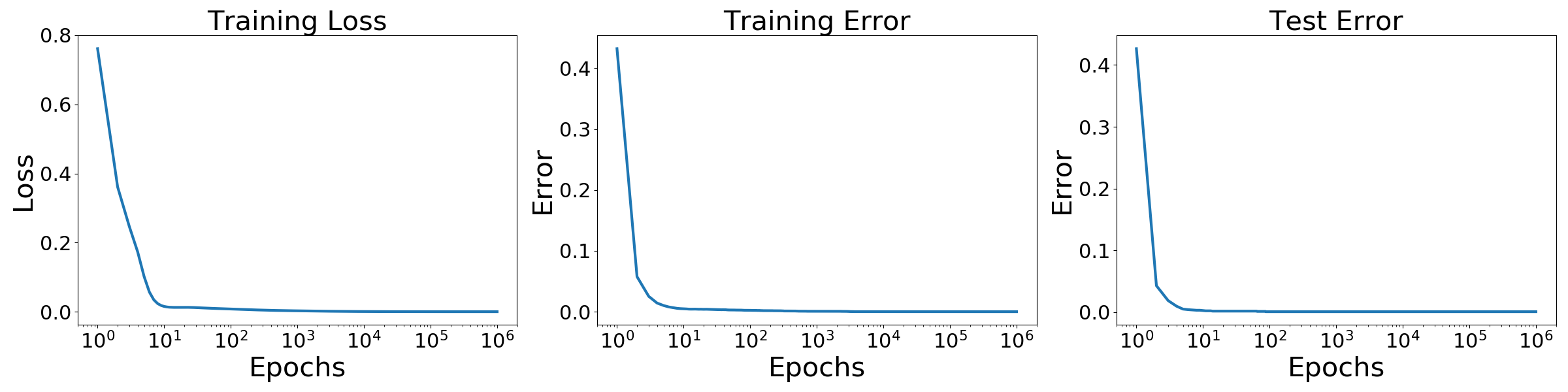
Figure 4. Training curves of logistic regression in Section 3 classifying $0$ and $1$ on MNIST. For the ease of illustration, x-axis is in log scale. Left: Training loss w.r.t. epochs. Middle: Training error w.r.t. epochs. Right: Test error w.r.t. epochs. The training error reaches zero, thus the subset of MNIST consisting of $0$’s and $1$’s is linear separable. Hence, this dataset strictly satisfies the contition in Theorem 1.

Figure 5 shows the training curves of six models in Section 5 by standarded training. Although there exists a generalization gap between training errors and test errors, the test errors never increase, thus the trade-off between minimum and average margin cannot be caused by overfitting.

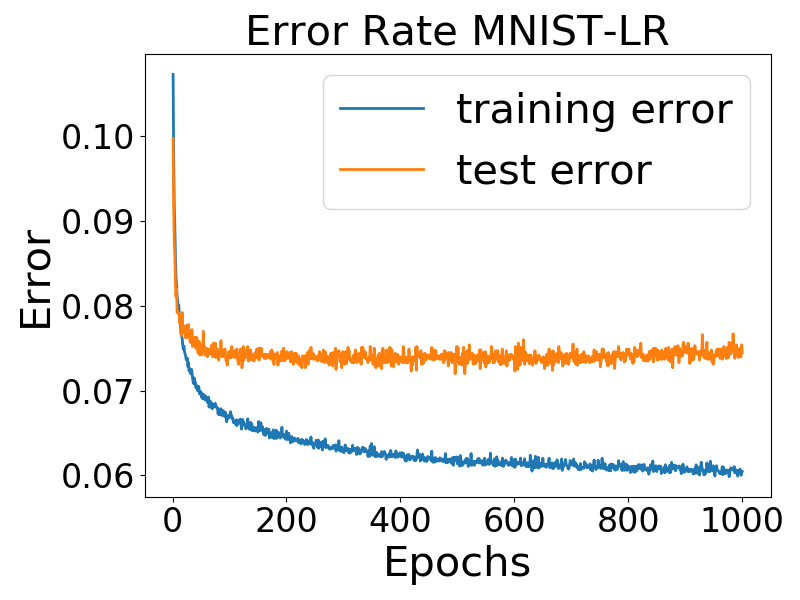
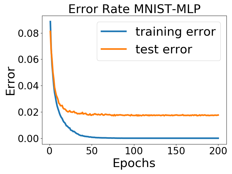
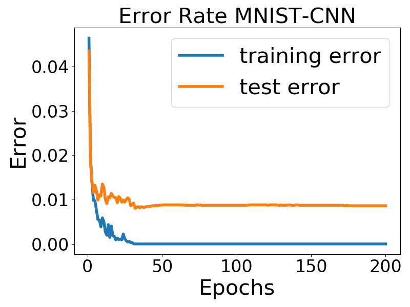
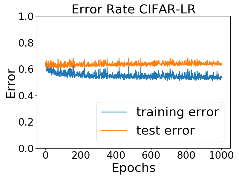
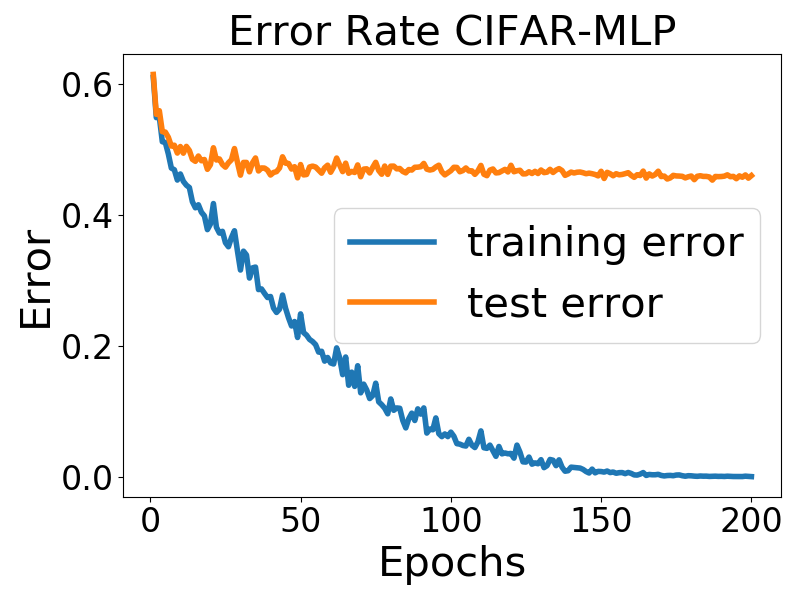
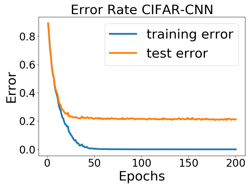
Figure 5. Training curves of 3 models on MNIST and 3 models on CIFAR10 by standard training. First Row : MNIST models. Second Row : CIFAR10 models.

Appendix C Minimum-average Margin Trade-off for MNIST Models

Figure 6 shows the minimum and average margin trade-off for MNIST models . A similar trade-off between minimum and average margin can be observed as discussed in Sections 3 and 5. The minimum margin keeps increasing while the average margin keeps decreasing. The only exception is the average margin of MNIST-CNN. But the range of margin in the figure is very small (from $0.94$ to $1.08$), in which case the Lipschitz constant estimation in Theorem 3 could be inaccurate.

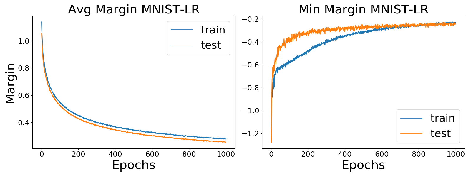
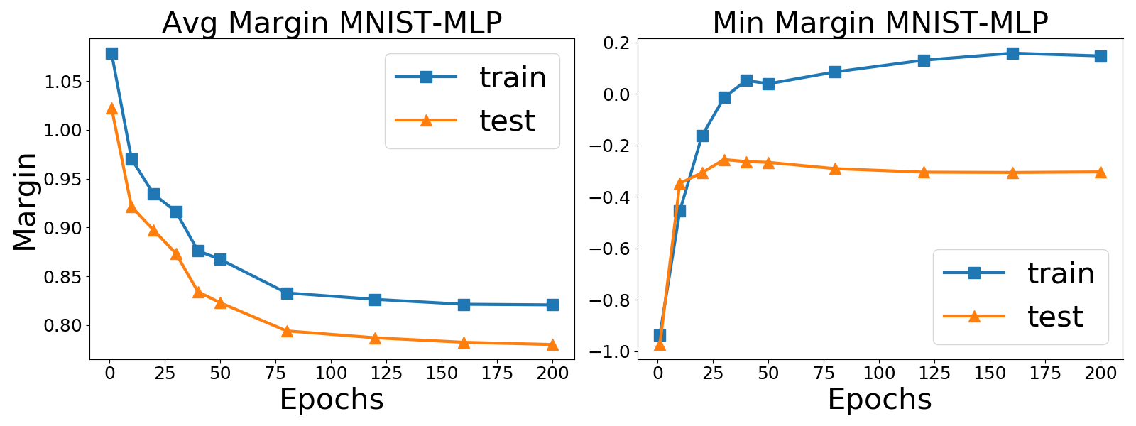
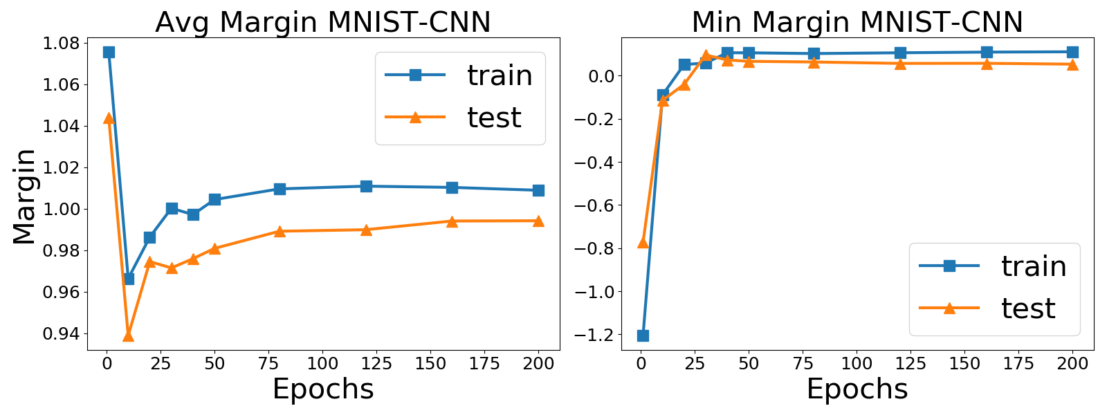
Figure 6. Average margin and minimum margin during training of 3 MNIST models.

Appendix D Margin Histograms of MNIST Models during Training

We plot margin histograms for three MNIST models in Figure 7.

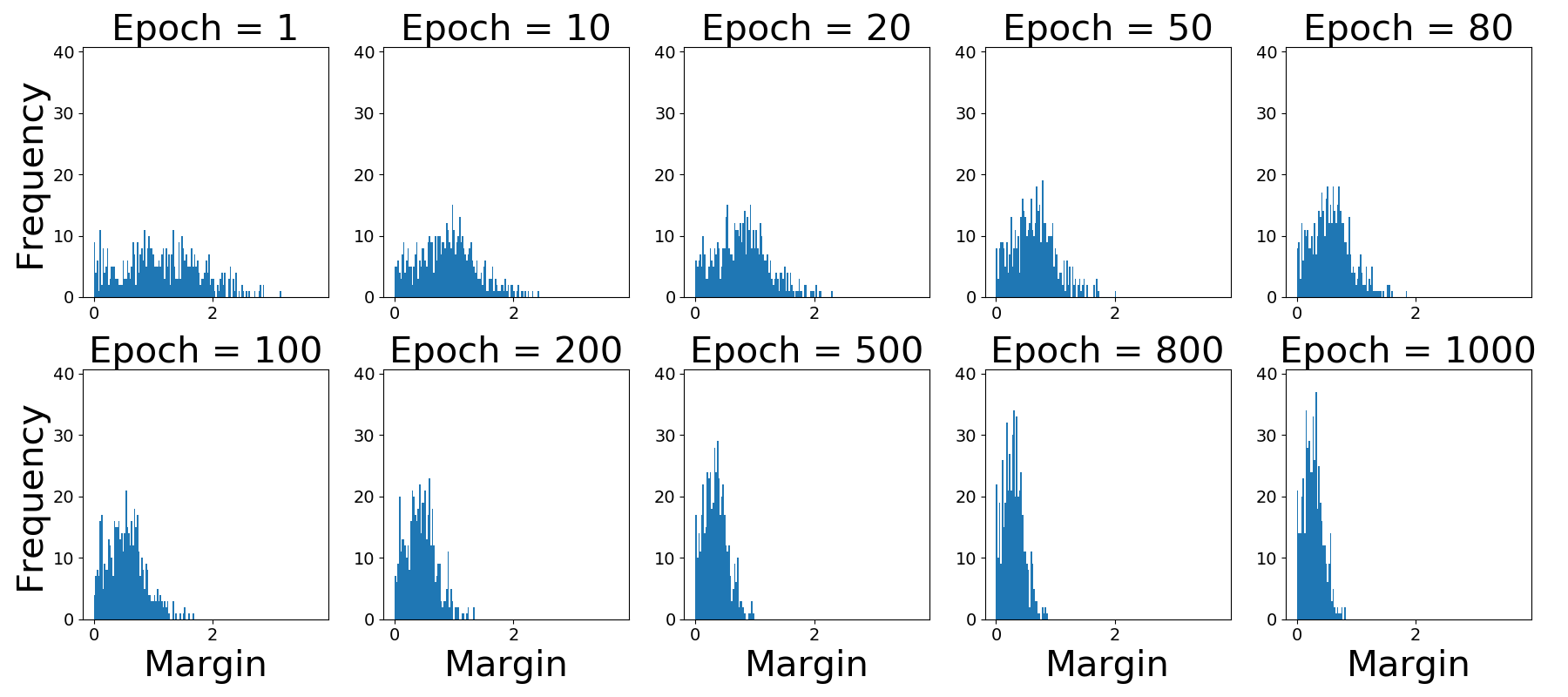
(a) Margin histograms of MNIST-LR on training set

(b) Margin histograms of MNIST-LR on test set

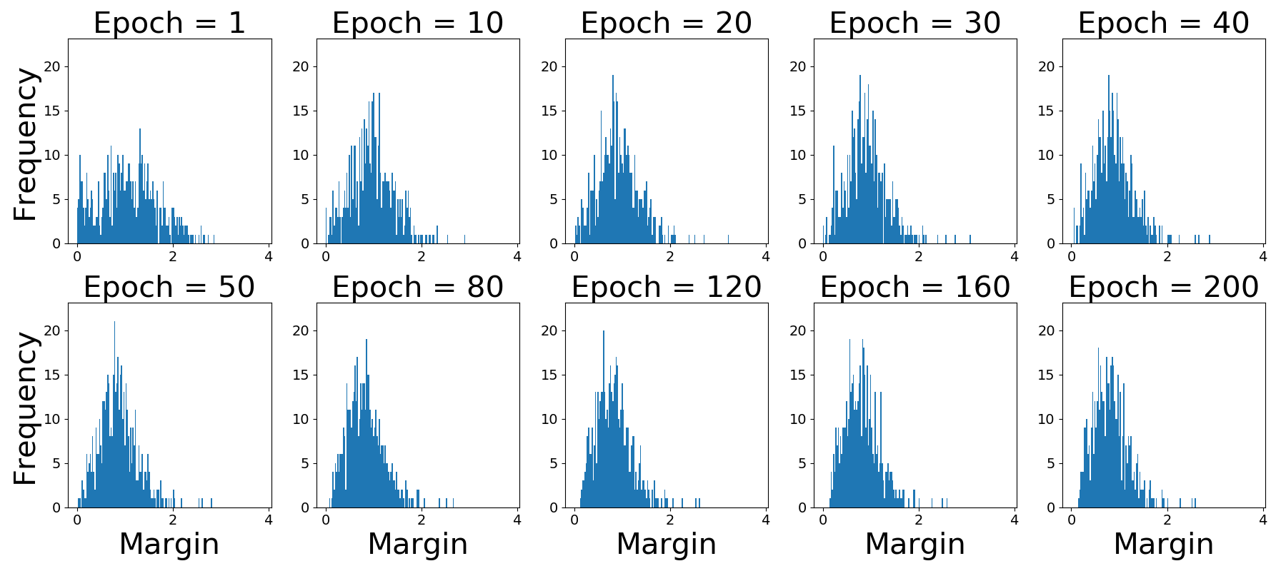
(c) Margin histograms of MNIST-MLP on training set

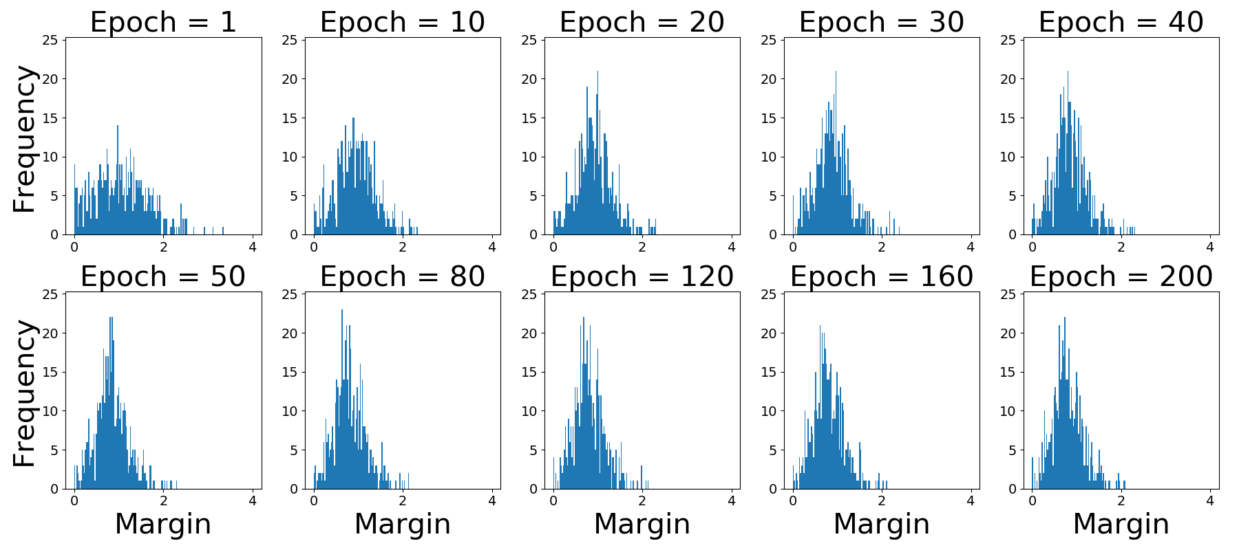
(d) Margin histograms of MNIST-MLP on test set

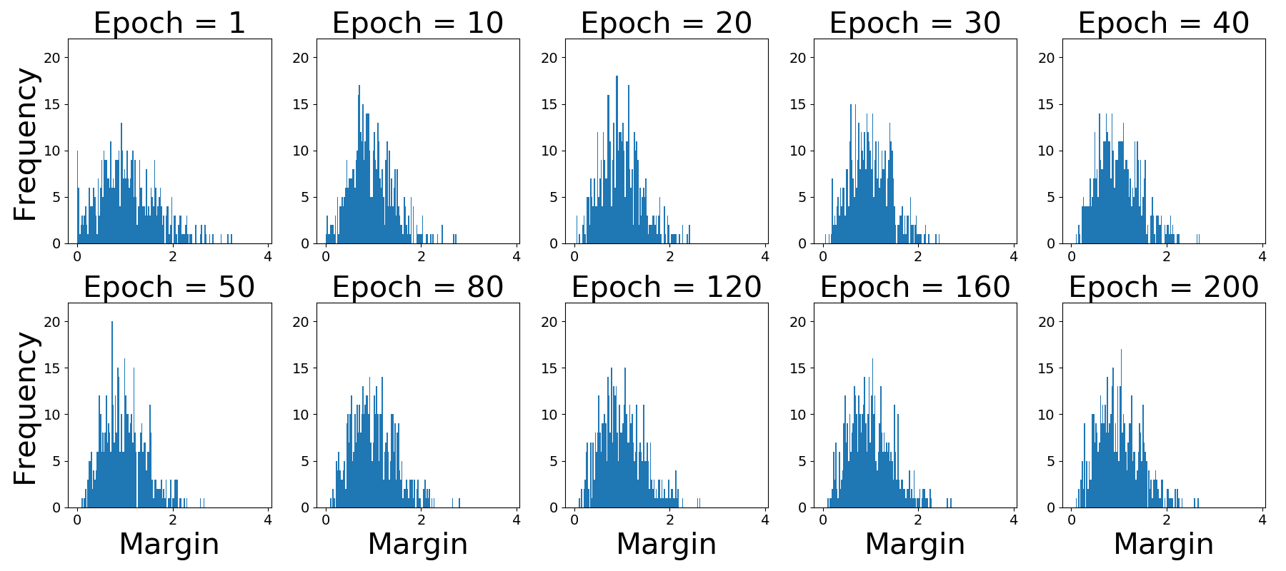
(e) Margin histograms of MNIST-CNN on training set

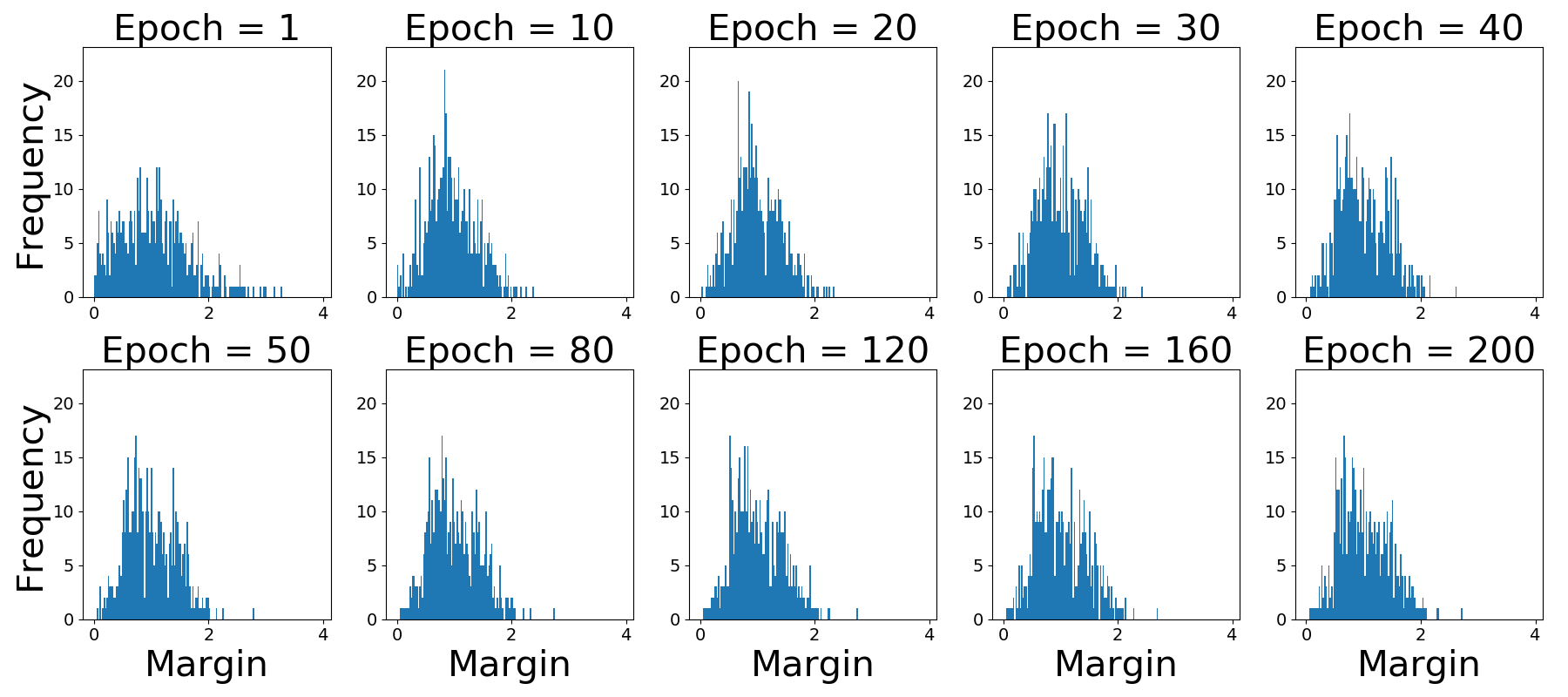
(f) Margin histograms of MNIST-CNN on test set

Figure 7. Margin histograms of MNIST models at different epochs during training. Top: Histograms of MNIST-LR. Mid: Histograms of MNIST-MLP. Bottom: Hostograms of MNIST-CNN.

Appendix E Margin Histograms of CIFAR Models during Training

We plot margin histograms for three CIFAR models in Figure 8.

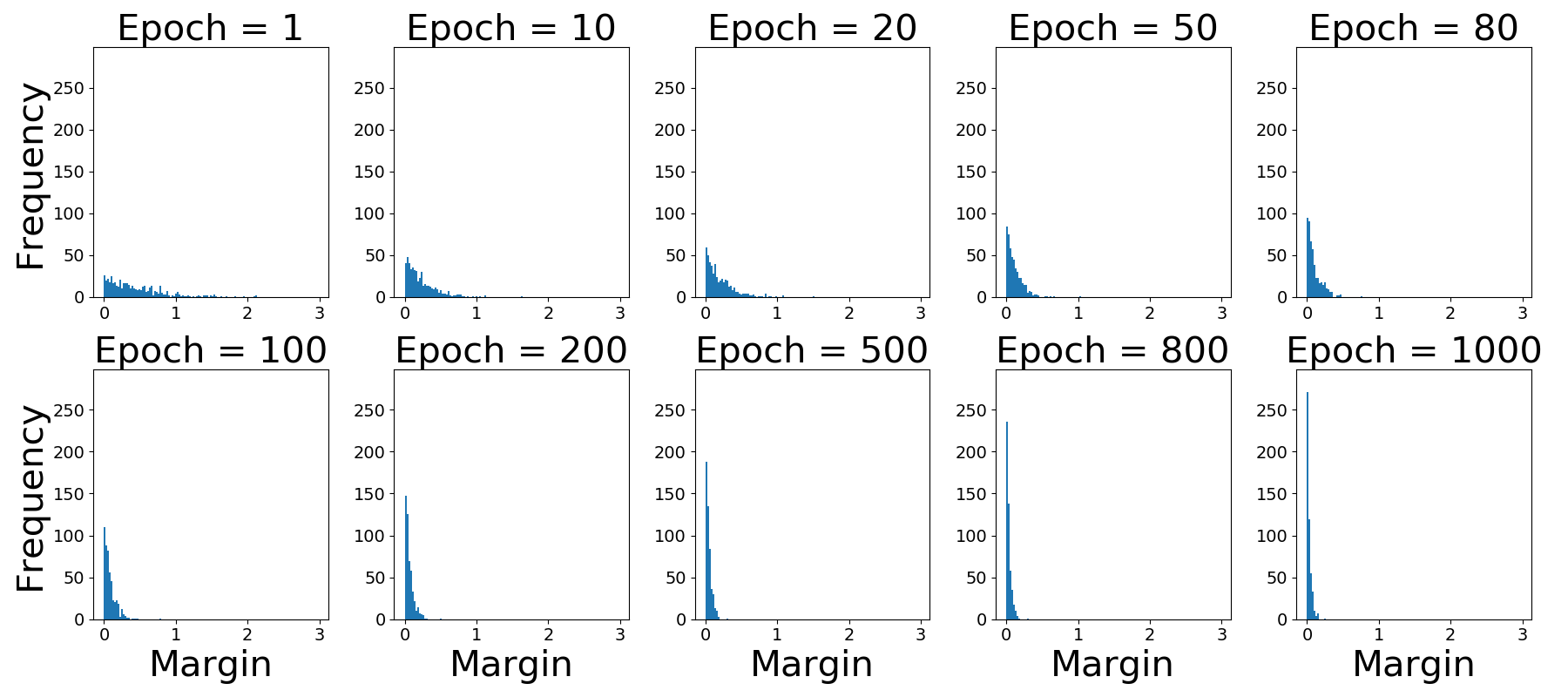
(a) Margin histograms of CIFAR-LR on training set

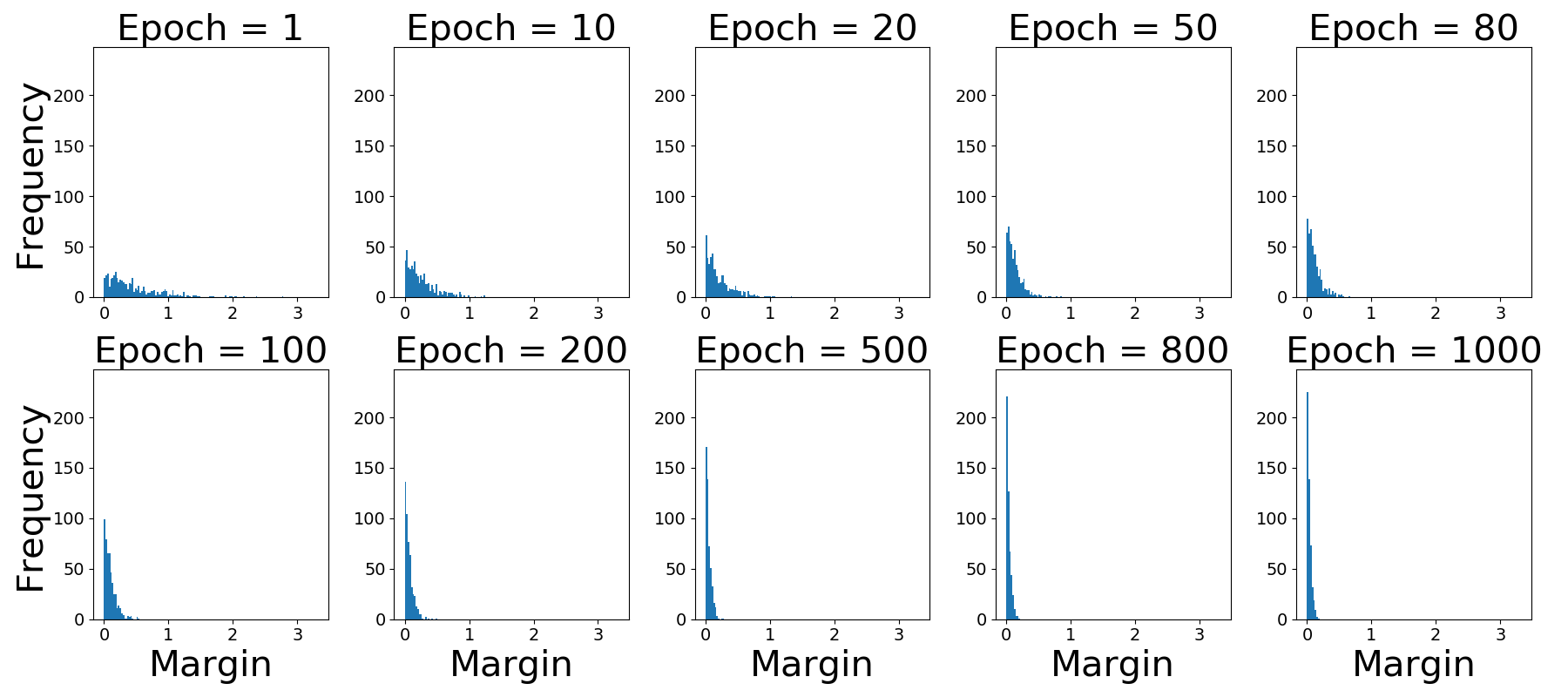
(b) Margin histograms of CIFAR-LR on test set

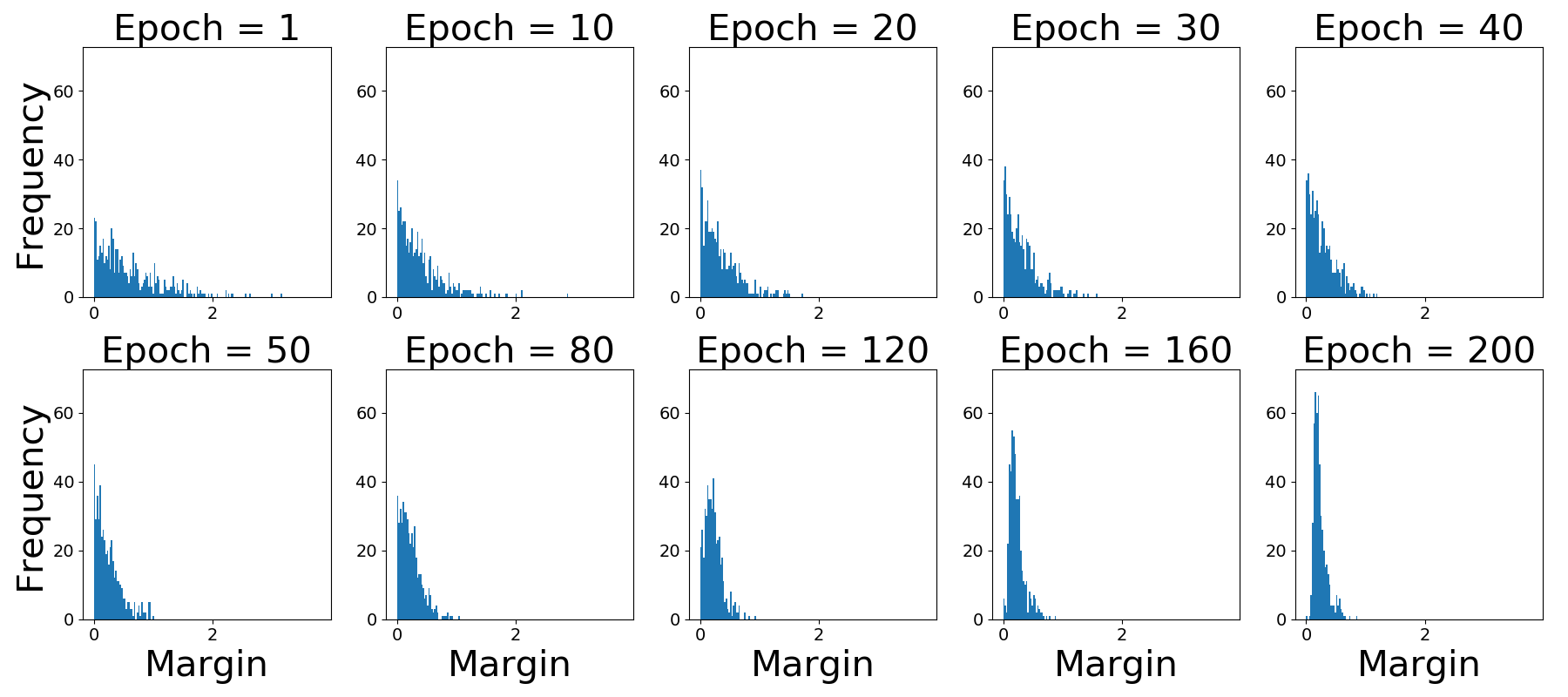
(c) Margin histograms of CIFAR-MLP on training set

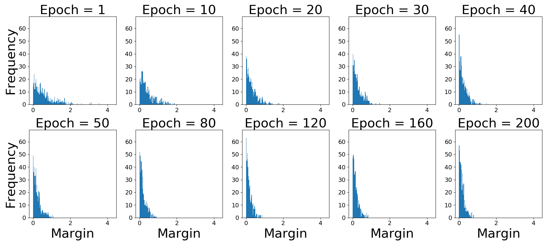
(d) Margin histograms of CIFAR-MLP on test set

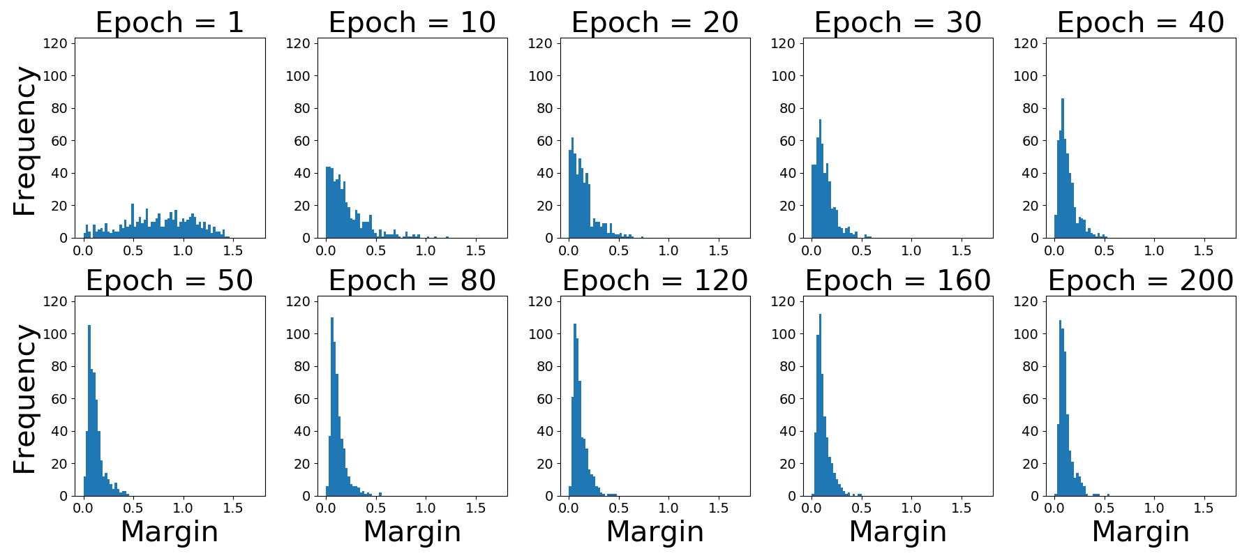
(e) Margin histograms of CIFAR-CNN on training set

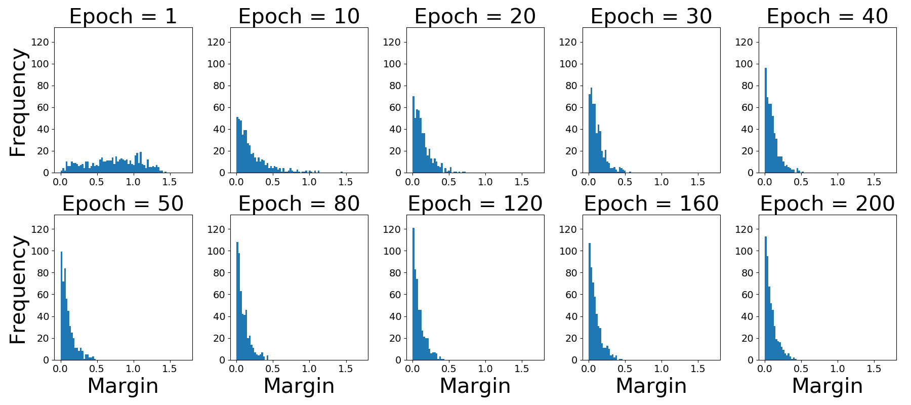
(f) Margin histograms of CIFAR-CNN on test set

Figure 8. Margin histograms of CIFAR models at different epochs during training. Top: Histograms of CIFAR-LR. Mid: Histograms of CIFAR-MLP. Bottom: Histograms of CIFAR-CNN.

Appendix F Detailed Experiment Setting

Model Architecture:

• MNIST-LR and CIFAR-LR: Multiclass logistic regression.

• MNIST-MLP and CIFAR-MLP: Neural network with one hidden layer. The hidden layer has $1024$ neurons and relu activation.

• MNIST-CNN and MNIST-CNN: Two AlexNet-Like convolutional neural networks with a slight difference. They are exactly the same as the models used by Weng et al. [17], Carlini and Wagner [4]. Dropout is used to alleviate overfitting on CIFAR10. No data augmentation is used.

• ConvNet: A convolutional neural network with $5$ convolutional layers, used in [36].

• LeNet: LeNet, consists of two convolutional layers and two fully connected layers.

• LeNetSmall: A convolutional neural network with similar structure to LeNet, but with fewer filers. This model is same as the one used in [35]. On CIFAR10, data augmentation (random crop and random flip) is used.

Standard Training: We use SGD (learning rate $0.01$) with momentum ($0.9$) and nestorv to train all six models. Batch size is set to $128$. Linear models (LR) are trained for $1000$ epochs. Nonlinear models (MLP, CNN) are trained for $200$ epochs.

Average Margin Regularizer: $\lambda=0.1$ and $\beta=10^{-3}$ are used for all models, while different $\tau$’s are used for different models. $\tau$ is tuned such that it is on the same order as the Lipschitz constant of the model. MNIST-LR and MNIST-MLP use $\tau=5$. MNIST-CNN use $\tau=10$. CIFAR-LR use $\tau=5$. CIFAR-MLP and CIFAR-CNN use $\tau=10$. The idea is using larger $\tau$ for deeper models. The spectral norm of weights across layers may not be exactly $1$, even after adding orthogonal constraint. In fact, the product of spectral norm will become larger as the model becomes deeper. Thus, one should use larger truncation parameter, since the range of margin in feature space may be larger. Following same idea, LeNet and LeNetSmall use $\tau=40$; ConvNet uses $\tau=50$.

In addition, for fair comparison, we set the same $\beta=10^{-3}$ to train models with Lipschitz constant regularization.

Adversarial Training: We use PGD attack to perform adversarial training. We set the number of iterations $40$ and step size $0.01$. On MNIST, the perturbation budget $\epsilon$ is set to $2.0$; on CIFAR, $\epsilon$ is set to $0.4$.

Attack Method: Through out the experiment, we use projected gradient descent (PGD) attack to evaluate the robust accuracy. We set step size $0.01$ and number of iterations $1000$. Increasing the number of iterations does not change the robust accuracy much, thus $1000$ iterations is sufficient to generate strong adversarial examples.

Approximating Distance When using Theorem 3 to approximate the distance to decision boundary, we need to estimation the Lipchitz constant of the network in a small neighbourhood around the input. Following [20], we simply take the maximum norm of gradient in that neighbourhood. Throughout the experiments, we set $r=5$ and the sampling size equal to $1024\times 50$ (except for linear classifiers, whose sampling size is $1$). For linear logistic regression, we perform estimation in every epoch; for nonlinear classifiers, we only perform estimation at certain epochs: $1$, $10$, $20$, $30$, $40$, $50$, $80$, $120$, $160$ and $200$, where we perform more estimations at the beginning, as distances may change drastically in initial stages. Due to efficiency concerns, the estimation is performed on a subset of size $500$, which is randomly chosen (with a fixed random seed) from the original training and test sets.

References

- Szegedy et al. [2014] Christian Szegedy, Wojciech Zaremba, Ilya Sutskever, Joan Bruna, Dumitru Erhan, Ian Goodfellow, and Rob Fergus. Intriguing properties of neural networks. In International Conference on Learning Representations (ICLR), 2014.
- Goodfellow et al. [2015] I. J. Goodfellow, J. Shlens, and C. Szegedy. Explaining and harnessing adversarial examples. In International Conference on Learning Representations (ICLR), 2015.
- Moosavi-Dezfooli et al. [2016] Seyed-Mohsen Moosavi-Dezfooli, Alhussein Fawzi, and Pascal Frossard. Deepfool: a simple and accurate method to fool deep neural networks. In Proceedings of the IEEE Conference on Computer Vision and Pattern Recognition, pages 2574–2582, 2016.
- Carlini and Wagner [2017] Nicholas Carlini and David Wagner. Towards evaluating the robustness of neural networks, 2017. arXiv:1608.
- Chen et al. [2017] Pin-Yu Chen, Huan Zhang, Yash Sharma, Jinfeng Yi, and Cho-Jui Hsieh. ZOO: Zeroth Order Optimization Based Black-box Attacks to Deep Neural Networks Without Training Substitute Models. In Proceedings of the 10th ACM Workshop on Artificial Intelligence and Security, pages 15–26, 2017.
- Hashemi et al. [2018] Mohammad Hashemi, Greg Cusack, and Eric Keller. Stochastic Substitute Training: A Gray-box Approach to Craft Adversarial Examples Against Gradient Obfuscation Defenses. In Proceedings of the 11th ACM Workshop on Artificial Intelligence and Security, pages 25–36, 2018.
- Du et al. [2018] Yali Du, Meng Fang, Jinfeng Yi, Jun Cheng, and Dacheng Tao. Towards Query Efficient Black-box Attacks: An Input-free Perspective. In Proceedings of the 11th ACM Workshop on Artificial Intelligence and Security, pages 13–24, 2018.
- Papernot et al. [2017] Nicolas Papernot, Patrick McDaniel, Ian Goodfellow, Somesh Jha, Z. Berkay Celik, and Ananthram Swami. Practical Black-Box Attacks Against Machine Learning. In Proceedings of the 2017 ACM on Asia Conference on Computer and Communications Security, pages 506–519, 2017.
- Zantedeschi et al. [2017] Valentina Zantedeschi, Maria-Irina Nicolae, and Ambrish Rawat. Efficient Defenses Against Adversarial Attacks. In Proceedings of the 10th ACM Workshop on Artificial Intelligence and Security, pages 39–49, 2017.
- Papernot et al. [2016] Nicolas Papernot, Patrick McDaniel, Xi Wu, Somesh Jha, and Ananthram Swami. Distillation as a defense to adversarial perturbations against deep neural networks. In IEEE Symposium on Security and Privacy, 2016.
- Cisse et al. [2017] Moustapha Cisse, Piotr Bojanowski, Edouard Grave, Yann Dauphin, and Nicolas Usunier. Parseval networks: Improving robustness to adversarial examples. In Proceedings of the 34th International Conference on Machine Learning, pages 854–863, 2017.
- Madry et al. [2018] Aleksander Madry, Aleksandar Makelov, Ludwig Schmidt, Dimitris Tsipras, and Adrian Vladu. Towards deep learning model resisstant to adversarial attacks. In International Conference on Learning Representations (ICLR), 2018.
- Goodfellow et al. [2018] Ian Goodfellow, Patrick McDaniel, and Nicolas Papernot. Making Machine Learning Robust Against Adversarial Inputs. Communications of the ACM, 61(7):56–66, 2018.
- Guo et al. [2018] Yiwen Guo, Chao Zhang, Changshui Zhang, and Yurong Chen. Sparse DNNs with Improved Adversarial Robustness. In Advances in Neural Information Processing Systems 31, pages 242–251, 2018.
- Athalye et al. [2018] Anish Athalye, Nicholas Carlini, and David Wagner. Obfuscated gradients give a false sense of security: Circumventing defenses to adversarial examples. In ICML, 2018.
- Hein and Andriushchenko [2017] Matthias Hein and Maksym Andriushchenko. Formal guarantees on the robustness of a classifier against adversarial manipulation. In Advances in Neural Information Processing Systems (NIPS), pages 2266–2276, 2017.
- Weng et al. [2018a] Tsui-Wei Weng, Huan Zhang, Pin-Yu Chen, Jinfeng Yi, Dong Su, Yupeng Gao, Cho-Jui Hsieh, and Luca Daniel. Evaluating the robustness of neural networks: An extreme value theory approach. In International Conference on Learning Representations (ICLR), 2018a.
- Zhang et al. [2018] Huan Zhang, Tsui-Wei Weng, Pin-Yu Chen, Cho-Jui Hsieh, and Luca Daniel. Efficient neural network robustness certification with general activation functions. In Advances in Neural Information Processing Systems, pages 4944–4953, 2018.
- Weng et al. [2018b] Tsui-Wei Weng, Huan Zhang, Hongge Chen, Zhao Song, Cho-Jui Hsieh, Duane Boning, Inderjit S. Dhillon, and Luca Daniel. Towards fast computation of certified robustness for relu networks. In ICML, 2018b.
- Tjeng et al. [2019] Vincent Tjeng, Kai Y. Xiao, and Russ Tedrake. Evaluating robustness of neural networks with mixed integer programming. In International Conference on Learning Representations, 2019.
- Singh et al. [2019] Gagandeep Singh, Timon Gehr, Markus Püschel, and Martin Vechev. Robustness certification with refinement. In International Conference on Learning Representations, 2019.
- Wong et al. [2018] Eric Wong, Frank Schmidt, Jan Hendrik Metzen, and J Zico Kolter. Scaling provable adversarial defenses. In Advances in Neural Information Processing Systems, pages 8400–8409, 2018.
- Wong and Kolter [2018] Eric Wong and J. Zico Kolter. Provable Defenses against Adversarial Examples via the Convex Outer Adversarial Polytope. In ICML, 2018.
- Raghunathan et al. [2018a] Aditi Raghunathan, Jacob Steinhardt, and Percy S Liang. Semidefinite relaxations for certifying robustness to adversarial examples. In Advances in Neural Information Processing Systems, pages 10900–10910, 2018a.
- Raghunathan et al. [2018b] Aditi Raghunathan, Jacob Steinhardt, and Percy Liang. Certified defenses against adversarial examples. In International Conference on Learning Representations, 2018b.
- Singh et al. [2018] Gagandeep Singh, Timon Gehr, Matthew Mirman, Markus Püschel, and Martin Vechev. Fast and Effective Robustness Certification. In Advances in Neural Information Processing Systems 31, pages 10802–10813. 2018.
- Gowal et al. [2018] Sven Gowal, Krishnamurthy Dvijotham, Robert Stanforth, Rudy Bunel, Chongli Qin, Jonathan Uesato, Relja Arandjelovic, Timothy Mann, and Pushmeet Kohli. On the Effectiveness of Interval Bound Propagation for Training Verifiably Robust Models. In NeurIPS workshop on Security in Machine Learning. 2018.
- Breiman [1999] Leo Breiman. Prediction Games and Arcing Algorithms. Neural Computation, 11(7):1493–1517, 1999.
- Schapire et al. [1998] Robert E. Schapire, Yoav Freund, Peter Bartlett, and Wee Sun Lee. Boosting the margin: a new explanation for the effectiveness of voting methods. The Annals of Statistics, 26(5):1651–1686, 1998.
- Garg et al. [2002] Ashutosh Garg, Sariel Har-Peled, and Dan Roth. On generalization bounds, projection profile, and margin distribution. In ICML, 2002.
- Garg and Roth [2003] Ashutosh Garg and Dan Roth. Margin distribution and learning algorithms. In ICML, 2003.
- Zhang and Zhou [2017] Teng Zhang and Zhi-Hua Zhou. Multi-class optimal margin distribution machine. In Proceedings of the 34th International Conference on Machine Learning-Volume 70, pages 4063–4071. JMLR. org, 2017.
- Soudry et al. [2018] Daniel Soudry, Elad Hoffer, and Nathan Srebro. The Implicit Bias of Gradient Descent on Separable Data. In International Conference on Learning Representations, 2018.
- Lee et al. [2019] Guang-He Lee, David Alvarez-Melis, and Tommi S. Jaakkola. Towards robust, locally linear deep networks. In International Conference on Learning Representations, 2019.
- Croce et al. [2019] Francesco Croce, Maksym Andriushchenko, and Matthias Hein. Provable robustness of relu networks via maximization of linear regions. In AISTATS, 2019.
- Yan et al. [2018] Ziang Yan, Yiwen Guo, and Changshui Zhang. Deep defense: Training dnns with improved adversarial robustness. In Advances in Neural Information Processing Systems, pages 419–428, 2018.
- Gunasekar et al. [2018] Suriya Gunasekar, Jason D Lee, Daniel Soudry, and Nati Srebro. Implicit bias of gradient descent on linear convolutional networks. In Advances in Neural Information Processing Systems, pages 9461–9471, 2018.
- Ji and Telgarsky [2019] Ziwei Ji and Matus Telgarsky. Gradient descent aligns the layers of deep linear networks. In International Conference on Learning Representations, 2019.
- Koltchinskii and Panchenko [2002] V. Koltchinskii and D. Panchenko. Empirical Margin Distributions and Bounding the Generalization Error of Combined Classifiers. The Annals of Statistics, 30(1):1–50, 2002.
- Bartlett et al. [2006] Peter L Bartlett, Michael I Jordan, and Jon D McAuliffe. Convexity, classification, and risk bounds. Journal of the American Statistical Association, 101(473):138–156, 2006.
- Katz et al. [2017] Guy Katz, Clark Barrett, David L. Dill, Kyle Julian, and Mykel J. Kochenderfer. Reluplex: An efficient smt solver for verifying deep neural networks. In International Conference on Computer Aided Verification, pages 97–117, 2017.
- Lin et al. [2019] Ji Lin, Chuang Gan, and Song Han. Defensive Quantization: When Efficiency Meets Robustness. In International Conference on Learning Representations, 2019.