Thermodynamic Geometry of the Quark-Meson Model

Abstract

We study the thermodynamic geometry of the Quark-Meson model, focusing on the curvature, $R$, around the chiral crossover at finite temperature and baryon chemical potential. We find a peculiar behavior of $R$ in the crossover region, in which the sign changes and a local maximum develops; in particular, the height of the peak of $R$ in the crossover region becomes large in proximity of the critical endpoint and diverges at the critical endpoint. The appearance of a pronounced peak of $R$ close to the critical endpoint supports the idea that $R$ grows with the correlation volume around the phase transition. We also analyze the mixed fluctuations of energy and baryon number, $\langle\Delta U\Delta N\rangle$, which grow up substantially in proximity of the critical endpoint: in the language of thermodynamic geometry these fluctuations are responsible for the vanishing of the determinant of the metric, which results in thermodynamic instability and are thus related to the appearance of the second order phase transition at the critical endpoint.

I Introduction

An interesting idea of Statistical Mechanics is that of a metric in the variety spanned by the thermodynamic variables: this is related to the theory of fluctuations among equilibrium states and lead to the concept of thermodynamic geometry and thermodynamic curvature Weinhold:1975get ; Weinhold:1975gtii ; Ruppeiner:1979trg ; Ruppeiner:1981agt ; Ruppeiner:1983ntp ; Ruppeiner:1983tcf ; Ruppeiner:1985cgt ; Ruppeiner:1985tcv ; Ruppeiner:1986tcv ; Ruppeiner:1990tig ; Ruppeiner:1990tof ; Ruppeiner:1991rgc ; Ruppeiner:1993afg ; Ruppeiner:1995rgf ; Ruppeiner:1998rgc ; Ruppeiner:2005rgr ; Ruppeiner:2008tcb ; Ruppeiner:2010tci ; Ruppeiner:2012tct ; Ruppeiner:2012tpw ; Ruppeiner:2013tfb ; Ruppeiner:2013tar ; Ruppeiner:2014utg ; Ruppeiner:2015trf ; Ruppeiner:2015tsf ; Ruppeiner:2015tsw ; Ruppeiner:2016smt ; Ruppeiner:2017svc ; Wei:2013ctb ; Janyszek:1989rtm ; Janyszek:1 ; Janyszek:2 ; Sahay:2017gcb ; Castorina:2018ayy ; Mirza:2009nta ; Mirza:2008rag ; Castorina:2018gsx ; Castorina:2019jzw ; Ruppeiner:maybe ; covariant:evolution ; geometrical:aspects ; crooks:measuring ; bellucci:PA . For example, in the grand-canonical ensemble the equilibrium state is specified as long as the intensive independent variables like temperature, chemical potential and others are fixed, and physical quantities like energy and particle number fluctuate with probability given by the Gibbs ensemble. Considering the pair of intensive variables $(\beta^{1},\beta^{2})$ the probability of a fluctuation from $S_{1}=(\beta^{1},\beta^{2})$ to $S_{2}=(\beta^{1}+d\beta^{1},\beta^{2}+d\beta^{2})$ is proportional to

$$\sqrt{g}\exp\left(-\frac{1}{2}g_{ij}d\beta^{i}d\beta^{j}\right),$$ (1)

where $g_{ij}\equiv\partial^{2}\log{\cal Z}/\partial\beta^{i}\partial\beta^{j}$ is called the thermodynamic metric tensor, $g=\mathrm{det}(g_{ij})$ is the determinant of $g_{ij}$ and ${\cal Z}$ is the grandcanonical partition function. It is therefore natural to define the line element $d\ell^{2}=g_{ij}d\beta^{i}d\beta^{j}$ which measures effectively a distance between $S_{1}$ and $S_{2}$, in the sense that a large $d\ell^{2}$ corresponds to a small probability of a fluctuation from $S_{1}$ to $S_{2}$. With the aid of $g_{ij}$ it is possible to define the thermodynamic curvature, $R=2R_{1212}/g$ with $g=\mathrm{det}(g_{ij})$ and $R_{1212}$ corresponding to the only independent component of the Riemann’s tensor for a two-dimensional variety. As it is clear from the very definition of $g_{ij}$, the thermodynamic curvature depends on the second and third order moments of the thermodynamic variables that are conjugated to $(\beta^{1},\beta^{2})$, therefore it carries information about the fluctuation of the physical quantities in particular around a phase transition, where these fluctuations are expected to be very large; for example, if $(\beta^{1},\beta^{2})=(1/T,-\mu/T)$ then $R$ contains information about the fluctuations of energy and particle number. One of the merits of the thermodynamic curvature is that in proximity of a second order phase transition $|R|\propto\xi^{d}$ where $d$ denotes the spatial dimension and $\xi$ is the correlation length: as a consequence, it is possible to grasp information about the correlation length by means of thermodynamics only. This divergence is related to the vanishing of the determinant of the metric, therefore the thermodynamic geometry gives information on the location of the phase transition in the $(\beta^{i})$ space.

The main purpose of this article is to report on our study about the thermodynamic geometry, and in particular on the thermodynamic curvature, of the Quark-Meson (QM) model of Quantum Chromodynamics (QCD), see Ruggieri:2013cya ; Ruggieri:2014bqa ; Frasca:2011zn ; Skokov:2010sf and references therein. It is well known that at zero baryon chemical potential, QCD matter experiences a smooth crossover from a low temperature confined phase in which chiral symmetry is spontaneously broken, to a high temperature phase in which color is deconfined and chiral symmetry is approximately restored Borsanyi:2013bia ; Bazavov:2011nk ; Cheng:2009zi ; Borsanyi:2010cj ; Borsanyi:2010bp . The situation is however unclear at finite baryon chemical potential for QCD with three colors, due to the sign problem that forbids first principle calculations. Because of this, effective models have been used to study the phase structure of QCD at finite $\mu$, and there is nowadays a consensus that regardless of the model used, the smooth crossover becomes a first order phase transition if $\mu$ is large enough: this leads to speculate the existence of a critical endpoint (CEP) in the $(T,\mu)$ plane at which the crossover becomes a true phase transition with divergent susceptibilities, and this point marks the separation between the crossover on the one hand and the first order line on the other hand. We consider here the QM model at finite $T$ and $\mu$, which has been applied many times to study the phase structure of QCD, and we study its thermodynamic geometry following the lines depicted in Castorina:2019jzw where a similar study has been performed for the Nambu-Jona-Lasinio (NJL) model. The advantage of using the QM model is its renormalizability, which removes the dependence of the results on the effective ultraviolet cutoff that instead appears in NJL calculations. Moreover, it is interesting to check how the predictions on the phase structure of QCD change when different effective models are used: this not only can shed light on the qualitative picture, but also put a quantitative statement on the theoretical uncertainty of model predictions, for example on the location of the CEP.

We can anticipate here the main results. The curvature is found to be negative at low temperature, as for an ideal fermion gas; then a change of sign is observed near the chiral crossover, where $R$ develops a local maximum which becomes more pronounced when the chemical potential is increased; finally, $R$ becomes negative again at high temperature and approaches zero from below. Moreover, the dependence of $R$ on temperature is nontrivial for large $\mu$ where two peaks are found in the crossover region, one negative at smaller temperature and one positive at higher temperature. Change of sign of $R$ has been observed for many substances Ruppeiner:2008tcb ; Ruppeiner:2012tct ; Ruppeiner:2013tar ; Ruppeiner:2013tfb ; Ruppeiner:2015tsf ; Ruppeiner:2015tsw ; Ruppeiner:2015trf ; Ruppeiner:2016smt ; Wei:2013ctb and it has been interpreted in terms of the nature of the attractive/repulsive microscopic interaction. In the case of the QM model it is difficult to support the relation between the nature of the interaction and the change of sign of $R$ since the interaction is always attractive: although mathematically the change of sign can be understood in terms of the different sign that accompanies the third order fluctuations in the expression of $R$, it is not clear if the change of sign of $R$ has any physical meaning in the model at hand and we think that this certainly deserves further study. Moreover, the height of the peak of $R$ increases along the critical line as $\mu$ is increased from zero to the corresponding CEP value and diverges at the CEP: this is in agreement with $|R|\propto\xi^{3}$ since the correlation length remains finite at the crossover but increases as the crossover becomes sharper and eventually diverges at the critical endpoint. We also discuss how the mixed susceptibility, $\langle\Delta U\Delta N\rangle$ which is nonzero at finite $\mu$, is crucial to have $g=0$ at the CEP.

The plan of the article is as follows. In Section II we briefly review the thermodynamic geometry and in particular the thermodynamic curvature. In Section III we review the QM model. In Section IV we discuss $R$ for the QM model. Finally, in Section V we draw our conclusions. We use the natural units system $\hbar=c=k_{B}=1$ throughout this article.

II Thermodynamic curvature

The idea of thermodynamic fluctuations, thermodynamic geometry and in particular of thermodynamic curvature is pretty old Weinhold:1975get ; Weinhold:1975gtii and is nowadays introduced on several textbooks of Statistical Mechanics, see for example Ruppeiner:maybe ; book:pathria ; book:landau . We present here only the few concepts that are closely related to our work, while we refer to Ruppeiner:1995rgf ; Ruppeiner:2010tci and references therein for more details.

Let us consider a thermodynamics system in the grand-canonical ensemble: we assume that its thermodynamic state at equilibrium is specified in terms of the coordinates $(T,\mu)$, where $T$ is the temperature and $\mu$ is the chemical potential conjugated to the particle density; alternatively we can use a different set of coordinates, namely $(\beta,\gamma)$ where $\beta=1/T$ and $\gamma=-\mu/T$. It is possible to build up a metric space in the $(\beta,\gamma)$ variety by defining a distance, namely

$$d\ell^{2}=g_{\beta\beta}d\beta d\beta+2g_{\beta\gamma}d\beta d\gamma+g_{\gamma\gamma}d\gamma d\gamma,$$ (2)

where for classical systems with grand-canonical partition function ${\cal Z}$ Janyszek:1989rtm

$$g_{ij}\equiv\frac{\partial\log{\cal Z}}{\partial\beta^{i}\partial\beta^{j}}=\frac{\partial\phi}{\partial\beta^{i}\partial\beta^{j}}\equiv\phi_{ij},$$ (3)

and $\phi\equiv\beta P$, $P=-\Omega$ with $\Omega$ representing the thermodynamic potential per unit volume; moreover, $\beta^{1}=1/T$, $\beta^{2}=\gamma=-\mu/T$. The line element $d\ell^{2}$ in Eq. (2) represents effectively a distance in the 2-dimensional variety, in the sense that the probability to fluctuate from the equilibrium state $S_{1}=(\beta,\gamma)$ to another equilibrium state $S_{2}=(\beta+d\beta,\gamma+d\gamma)$ is

$$\frac{dP}{d\beta d\gamma}\propto\sqrt{g}\exp\left(-\frac{d\ell^{2}}{2}\right);$$ (4)

therefore, the larger the distance the less probable is to have a fluctuation from $S_{1}$ to $S_{2}$ and the two states are effectively distant. In the above equation $g$ denotes the determinant of the metric tensor in Eq. (3). With these definitions the thermodynamic curvature of the 2-dimensional variety is given by

$$R=-\frac{1}{2g^{2}}\left|\begin{array}[]{ccc}\phi_{\beta\beta}&\phi_{\beta\gamma}&\phi_{\gamma\gamma}\\ \phi_{\beta\beta\beta}&\phi_{\beta\beta\gamma}&\phi_{\beta\gamma\gamma}\\ \phi_{\beta\beta\gamma}&\phi_{\beta\gamma\gamma}&\phi_{\gamma\gamma\gamma}\end{array}\right|,$$ (5)

where $||$ means the determinant of the $3\times 3$ matrix and

$$\phi_{ij}=\langle(F_{i}-\langle F_{i}\rangle)(F_{j}-\langle F_{j}\rangle)\rangle,$$ (6)

$$\phi_{ijk}\equiv\frac{\partial\phi_{jk}}{\partial\beta^{i}}=-\langle(F_{i}-\langle F_{i}\rangle)(F_{j}-\langle F_{j}\rangle)(F_{k}-\langle F_{k}\rangle)\rangle,$$

where $F_{i}$ denotes the physical quantity conjugated to $\beta^{i}$ and $\langle\rangle$ is the standard ensemble average. We notice that our sign convention agrees with Janyszek:1989rtm , in particular $R>0$ for the sphere. For our choice of coordinates we have, for example Janyszek:1 ,

$$\phi_{\beta\beta}=\langle(U-\langle U\rangle)^{2}\rangle,$$ (8)

$$\phi_{\beta\gamma}=\langle(U-\langle U\rangle)(N-\langle N\rangle)\rangle,$$ (9)

$$\phi_{\gamma\gamma}=\langle(N-\langle N\rangle)^{2}\rangle,$$ (10)

where $U$, $N$ denote the internal energy and the particle number respectively. The diagonal matrix elements $\phi_{\beta\beta}$ and $\phi_{\gamma\gamma}$, are related to the specific heat and the isothermal compressibility, $\chi_{T}$, respectively Janyszek:1 , namely

$$\beta^{2}\phi_{\beta\beta}=\left(\frac{\partial U}{\partial T}\right)_{\gamma},$$ (11)

$$\beta\phi_{\gamma\gamma}=\frac{N^{2}}{V}\chi_{T},$$ (12)

where $\chi_{T}=-(\partial V/\partial P)_{T}$. Similarly, we can write

$$\phi_{\beta\beta\beta}=-\langle(U-\langle U\rangle)^{3}\rangle,$$ (13)

$$\phi_{\gamma\gamma\gamma}=-\langle(N-\langle N\rangle)^{3}\rangle.$$ (14)

The thermodynamic curvature has the merit that close to a phase transition $|R|\propto\xi^{3}$ in three spatial dimensions, where $\xi$ corresponds to the correlation length. Therefore, in principle it is possible to access to microscopic details like $\xi$ in the proximity of the phase transition just by means of thermodynamics. Within our sign convention, $R<0$ for an ideal fermion gas and $R>0$ for an ideal boson gas; $R=0$ for the ideal classical gas; for anyon gases Mirza:2008rag ; Mirza:2009nta it is possible to deform continuously the distribution from a fermionic to a bosonic one, and this results in a change of the sign of $R$ in agreement with the previous statement. For interacting systems the interpretation of the sign of $R$ is far more complicated and nowadays there is no consensus on what this sign means. For example, for many substances it has been found that $R<0$, but for these there exist a range of temperature/density in which $R>0$ and this change of sign has been interpreted as a transition from a fluid to a solid-like fluid behavior Ruppeiner:2012tct ; Ruppeiner:2015trf . In addition to this, it has been found that $R>0$ if the attractive interaction dominates, while $R<0$ if the repulsive interaction is more important Ruppeiner:2013tar : while this seems to be satisfied by several substances, it is unclear if this relation between the sign of $R$ and the nature of the interaction is general.

III The quark-meson model

The QM model is an effective model of QCD in which quarks and mesons are considered on the same footing; it is a very well known model in Quantum Field Theory, where it is called the linear-sigma model coupled to fermions (see e.g. Peskin:1995ev ; Weinberg:1996kr ). The meson part of the lagrangian density of the QM model is

$${\cal L}_{\mathrm{mesons}}=\frac{1}{2}\left(\partial^{\mu}\sigma\partial_{\mu}\sigma+\partial^{\mu}\bm{\pi}\cdot\partial_{\mu}\bm{\pi}\right)-\frac{\lambda}{4}\left(\sigma^{2}+\bm{\pi}^{2}-v^{2}\right)^{2}+h\sigma,$$ (15)

where $\bm{\pi}=(\pi_{1},\pi_{2},\pi_{3})$ corresponds to the pion isotriplet field. This lagrangian density is invariant under $O(4)$ rotations. On the other hand, as long as $v^{2}>0$ the potential develops an infinite set of degenerate minima. We choose one ground state, namely

$$\langle\bm{\pi}\rangle=0,\leavevmode\nobreak\ \leavevmode\nobreak\ \langle\sigma\rangle=v=F_{\pi},$$ (16)

where $F_{\pi}\approx 93$ MeV denotes the pion decay constant. The ground state specified in Eq. (16) breaks the $O(4)$ symmetry down to $O(3)$ since the vacuum is invariant only under the rotations of the pion fields. The quark sector of the QM model is described by the lagrangian density

$${\cal L}_{\mathrm{quarks}}=\bar{\psi}\left(i\partial_{\mu}\gamma^{\mu}-G(\sigma+i\gamma_{5}\bm{\pi}\cdot\bm{\tau})\right)\psi,$$ (17)

where $\bm{\tau}$ are Pauli matrices in the flavor space. In the ground state (16) quarks get a dynamical (that is, a constituent) mass given by

$$M_{q}=G\langle\sigma\rangle=GF_{\pi}.$$ (18)

We notice that in Eq. (17) there is no explicit mass term for the quarks. As a matter of fact, in this effective model the explicit breaking of chiral symmetry is achieved by the term

$${\cal L}_{\mathrm{mass}}=h\sigma$$ (19)

in Eq. (15). In the limit $h/F_{\pi}^{3}\ll 1$ this implies $F_{\pi}M_{\pi}^{2}=h$. Although in Eq. (17) there is no explicit mass term, quarks get a constituent mass because of the spontaneous breaking of the $O(4)$ symmetry in the meson sector: this implies that the quark chiral condensate can be nonzero. Finally,

$${\cal L}_{\mathrm{QM}}={\cal L}_{\mathrm{quarks}}+{\cal L}_{\mathrm{mesons}}.$$ (20)

The mean field effective potential of the QM model at zero temperature is given by

$$\Omega=U+\Omega_{q},$$ (21)

where

$$U=\frac{\lambda}{4}\left(\sigma^{2}+\bm{\pi}^{2}-v^{2}\right)^{2}-h\sigma,$$ (22)

is the classical potential of the meson fields as it can be read from Eq. (15) and

$$\Omega_{q}=-2N_{c}N_{f}\int\frac{d^{3}p}{(2\pi)^{3}}E_{p}$$ (23)

is the one-loop quark contribution, with

$$E_{p}=\sqrt{p^{2}+M^{2}},\leavevmode\nobreak\ \leavevmode\nobreak\ \leavevmode\nobreak\ M=G\sigma.$$ (24)

We notice that the quark mass depends on the field $\sigma$, thus Eq. (21) is the effective potential for the $\sigma$ field computed at one-loop and after regularization it corresponds to the condensation energy, namely the difference between the energy of the state with $\langle\sigma\rangle\neq 0$ and $\langle\sigma\rangle=0$ at $T=0$.

The quark loop in Eq. (23) is divergent in the ultraviolet (UV) but the QM model is renormalizable, therefore we can apply a strandard renormalization procedure to remove this divergence. To this end we introduce the function Ruggieri:2013cya ; Ruggieri:2014bqa ; Frasca:2011zn

$$\Omega_{q}(s)=-2N_{c}N_{f}\nu^{2s}\int\frac{d^{3}p}{(2\pi)^{3}}\left(p^{2}+M^{2}\right)^{\frac{1}{2}-s},$$ (25)

where $s$ is a complex number and $\nu$ carries the dimension of a mass in order to balance the wrong mass dimension of the integrand when $s\neq 0$. The strategy is to compute the above integral for a finite value of $s$, then make analytical continuation to $s=0$. The integral can be performed analytically with the result

$$\Omega_{q}(s)=-\frac{N_{c}N_{f}}{4\pi^{3/2}}\nu^{2s}M^{4-2s}\frac{\Gamma(s-2)}{\Gamma\left(s-\frac{1}{2}\right)},$$ (26)

where $\Gamma$ denotes the standard Euler’s function. In the limit $s\rightarrow 0^{+}$ we get

$$\Omega_{q}(s)=-\frac{N_{c}N_{f}}{2\pi^{2}}\left[-\frac{M^{4}}{8s}+\frac{M^{4}}{16}\left(-3+2\gamma_{E}+2\psi(-1/2)+4\log\frac{M}{\nu}\right)\right],$$ (27)

where $\psi(z)=d\log\Gamma(z)/dz$ and $\gamma_{E}\approx 0.577$ is the Euler constant. We notice that the UV divergence is now manifest in the analytical structure of $\Omega_{q}(s)$ in the complex plane, namely it appears as a simple pole at $s=0$.

We now add two counterterms,

$$\Omega_{\mathrm{ct}}=\frac{\delta v}{2}\sigma^{2}+\frac{\delta\lambda}{4}\sigma^{4},$$ (28)

to the quark loop and require that the renormalized quark loop does not shift the values of the $\sigma$ meson mass as well as the value of the condensate obtained within the classical potential (16); $\delta v$ and $\delta\lambda$ will absorb the divergence of $\Omega_{q}$ and the final result will be a convergent quantity. By definining the renormalized potential as

$$\Omega_{q}^{\mathrm{ren}}=\Omega_{q}+\Omega_{\mathrm{ct}}$$ (29)

the renormalization conditions thus read

$$\left.\frac{\partial\Omega_{q}^{\mathrm{ren}}}{\partial\sigma}\right|_{\sigma=v}=0,\leavevmode\nobreak\ \leavevmode\nobreak\ \left.\frac{\partial^{2}\Omega_{q}^{\mathrm{ren}}}{\partial\sigma^{2}}\right|_{\sigma=v}=0;$$ (30)

as a matter of fact, the first condition implies that $\Omega_{q}^{\mathrm{ren}}$ does not shift the global minimum of the effective potential, and this will be given by the minimum of the classical potential, while the second condition implies that for $\sigma=v$, namely in the ground state, the mass matrix of the $\sigma$ meson is not affected by the quark loop. The counterterms can be computed very easily and their expression is not necessary here, therefore we write directly the expression for the renormalized potential, namely

$$\Omega_{q}^{\mathrm{ren}}=\frac{3G^{4}}{32\pi^{2}}N_{c}N_{f}\sigma^{4}-\frac{G^{4}F_{\pi}^{2}}{8\pi^{2}}N_{c}N_{f}\sigma^{2}+\frac{G^{4}N_{c}N_{f}}{8\pi^{2}}\sigma^{4}\log\frac{F_{\pi}}{\sigma}.$$ (31)

We notice that $\Omega_{q}^{\mathrm{ren}}=0$ for $\sigma=0$ and that $\Omega_{q}^{\mathrm{ren}}=-G^{4}F_{\pi}^{4}N_{c}N_{f}/32\pi^{2}$ for $\sigma=F_{\pi}$: thus, $\Omega_{q}^{\mathrm{ren}}$ lowers the energy difference between the states with and without a condensate.

The finite temperature thermodynamic potential is finite and does not need any particular treatment: it is given by the standard relativistic fermion gas contribution, namely

$$\Omega_{T}=-2N_{c}N_{f}T\int\frac{d^{3}p}{(2\pi)^{3}}\log\left(1+e^{-\beta(E_{p}-\mu)}\right)\left(1+e^{-\beta(E_{p}+\mu)}\right),$$ (32)

where $\mu$ corresponds to the chemical potential and $E_{p}=\sqrt{p^{2}+M^{2}}$ with $M=g\sigma$. Putting all together we get

$$\Omega = U(\sigma)+\frac{3G^{4}}{32\pi^{2}}N_{c}N_{f}\sigma^{4}-\frac{G^{4}F_{\pi}^{2}}{8\pi^{2}}N_{c}N_{f}\sigma^{2}+\frac{G^{4}N_{c}N_{f}}{8\pi^{2}}\sigma^{4}\log\frac{F_{\pi}}{\sigma}$$ (33)

$$-2N_{c}N_{f}T\int\frac{d^{3}p}{(2\pi)^{3}}\log\left(1+e^{-\beta(E_{p}-\mu)}\right)\left(1+e^{-\beta(E_{p}+\mu)}\right).$$

The pressure is $P(T,\mu)=-\Omega(T,\mu,\bar{\sigma})$ where $\bar{\sigma}$ is the value of $\sigma$ that minimizes $\Omega$ at a given $(T,\mu)$.

IV Results

IV.1 The thermodynamic curvature

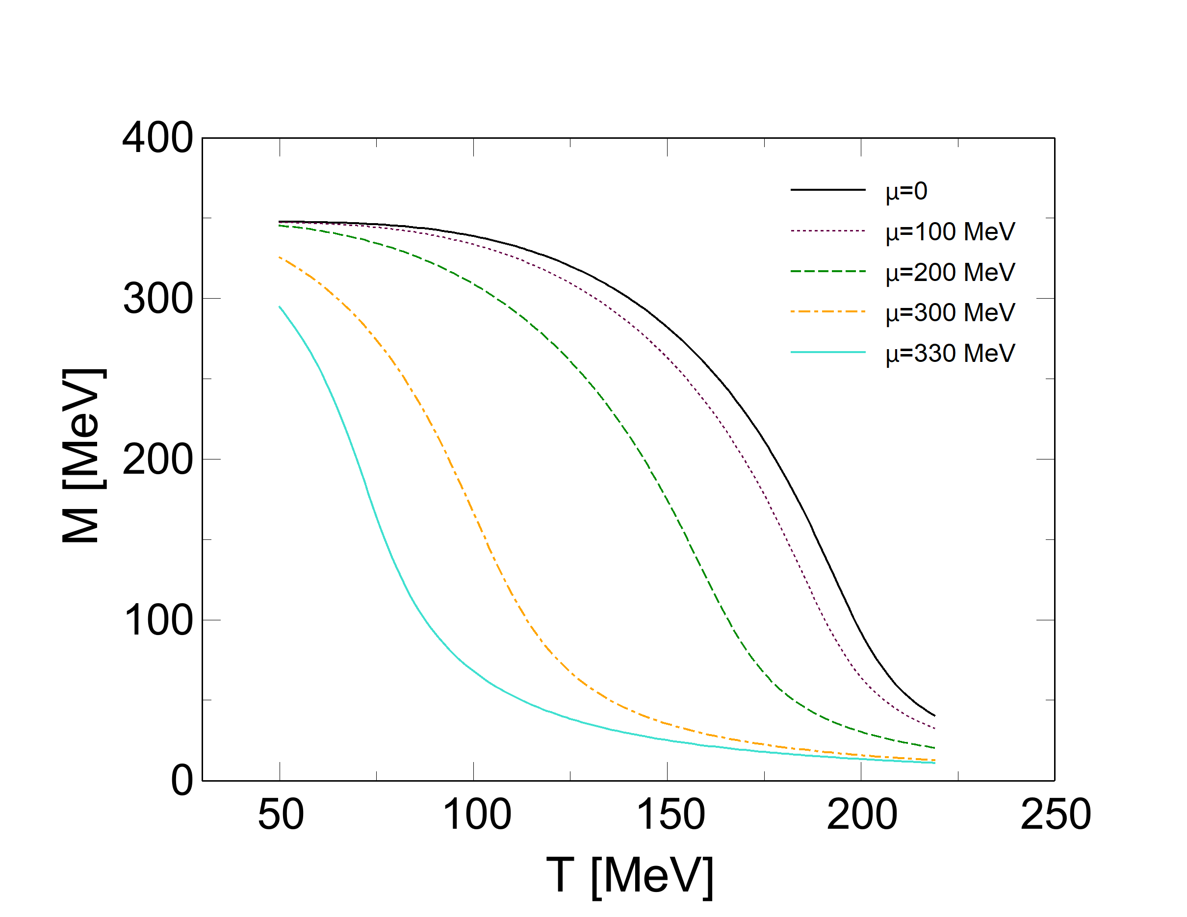
Figure 1: Constituent quark mass, $M$, versus temperature for several values of the quark chemical potential: black solid line is for $\mu=0$, brown dotted line denotes $\mu=100$ MeV, green dashed line stands for $\mu=200$ MeV, orange dot-dashed line corresponds to $\mu=300$ MeV and finally turquoise solid line stands for $\mu=330$ MeV.

In this section we summarize the results we have obtained for the QM model. Our parameter set is $M_{\sigma}=700$ MeV, $v=F_{\pi}=93$ MeV, $M_{\pi}=138$ MeV and $G=3.6$; these give $M=335$ MeV at $T=0$ and $\mu=0$, $\lambda=M_{\sigma}^{2}/2F_{\pi}^{2}=28.3$ and $h=M_{\pi}^{2}F_{\pi}=1.78\times 10^{6}$ MeV³. We have also used another parameter set with $M_{\sigma}=600$ MeV and $M=350$ MeV at $\mu=T=0$ but the results are unchanged qualitatively, therefore we present here only the results related to the first parameter set.

In Fig. 1 we plot the constituent quark mass as a function of temperature for several values of the quark chemical potential: black solid line is for $\mu=0$, brown dotted line denotes $\mu=100$ MeV, green dashed line stands for $\mu=200$ MeV, orange dot-dashed line corresponds to $\mu=300$ MeV and finally turquoise solid line stands for $\mu=330$ MeV. For any value of $\mu$ there exists a range of temperature in which $M$ decreases: this is the chiral crossover from a low temperature phase with spontaneous chiral symmetry breaking from a high temperature phase in which chiral symmetry is approximately restored. The larger $\mu$ the sharper the change of $M$ with $T$ is, and for $(T,\mu)\equiv(T_{E},\mu_{E})\approx(30\leavevmode\nobreak\ \mathrm{MeV},360\leavevmode\nobreak\ \mathrm{MeV})$ we find the critical endpoint (CEP) at which the crossover becomes a true second order phase transition and for $\mu>\mu_{E}$ the phase transition is a first order one.

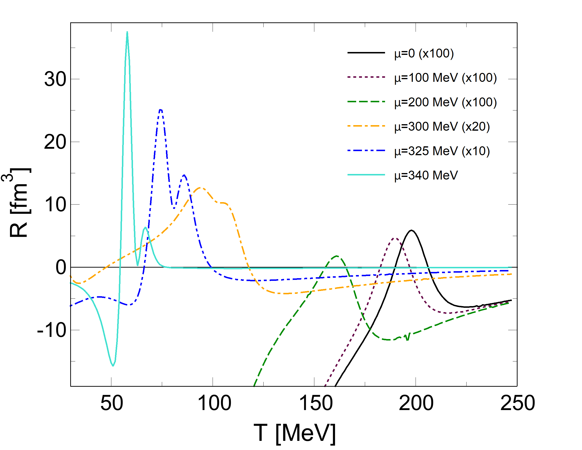
Figure 2: Thermodynamic curvature, $R$, versus temperature for several values of the quark chemical potential: black solid line is for $\mu=0$, brown dotted line denotes $\mu=100$ MeV, green dashed line stands for $\mu=200$ MeV, orange dot-dashed line corresponds to $\mu=300$ MeV, blue dot-dot-dashed line denotes $\mu=325$ MeV and finally turquoise solid line stands for $\mu=340$ MeV.

In Fig. 2 we plot the thermodynamic curvature, $R$, versus temperature for several values of the quark chemical potential: black solid line is for $\mu=0$, brown dotted line denotes $\mu=100$ MeV, green dashed line stands for $\mu=200$ MeV, orange dot-dashed line corresponds to $\mu=300$ MeV, blue dot-dot-dashed line denotes $\mu=325$ MeV and finally turquoise solid line stands for $\mu=340$ MeV. At small temperature the curvature is negative, as for a free fermion gas. However, we notice that the sign of $R$ changes around the crossover, then becoming negative again for $T\gg T_{c}$: the crossover corresponds to a change in the geometry from hyperbolic to elliptic Saccheri ; Beltrami:1828 ; book:1 ; Lobachevsky:1829 . Following Castorina:2019jzw we identify the region in which $R>0$ with the crossover. This interpretation is supported by the fact that the local maxima of $R$ appear to be very close to those of $|dM/dT|$, the latter giving a rough location of the crossover itself, see also below. The fact that the magnitude of $R$ in the critical region remains small for small $\mu$ is related to the fact that in this region the crossover is very smooth; on the other hand, when we approach the critical endpoint the crossover is closer to a second order phase transition and $R$ develops clear peaks.

We also notice that the structure of $R(T)$ as the critical endpoint is approached is quite interesting. Indeed, for $\mu=340$ MeV in Fig. 2 we find that $R$ is negative and drops down before rising to a positive peak around the crossover. The behavior of $R$ that we find can be understood mathematically since $R$ combines several second and third order cumulants with different signs, see Section II. Overall, the increase of the magnitude of $R$ as the CEP is approached is due to the determinant of the metric that becomes small around CEP and eventually vanishes at the CEP, see below. We also notice that increasing the temperature right above the peak results in $R=0$ then $R$ stays positive for a substantial temperature range, before becoming negative again: the $R=0$ point can be understood since $\phi_{\beta\beta\beta}$, $\phi_{\beta\beta\gamma}$, $\phi_{\beta\gamma\gamma}$ and $\phi_{\gamma\gamma\gamma}$ vanish at that temperature and so $R$ does: this is in agreement with well known fact that the third order cumulants change sign around the critical endpoint Vovchenko:2015pya ; Li:2017ple ; Li:2018ygx ; Shao:2017yzv

IV.2 The thermodynamic geometry at the critical line

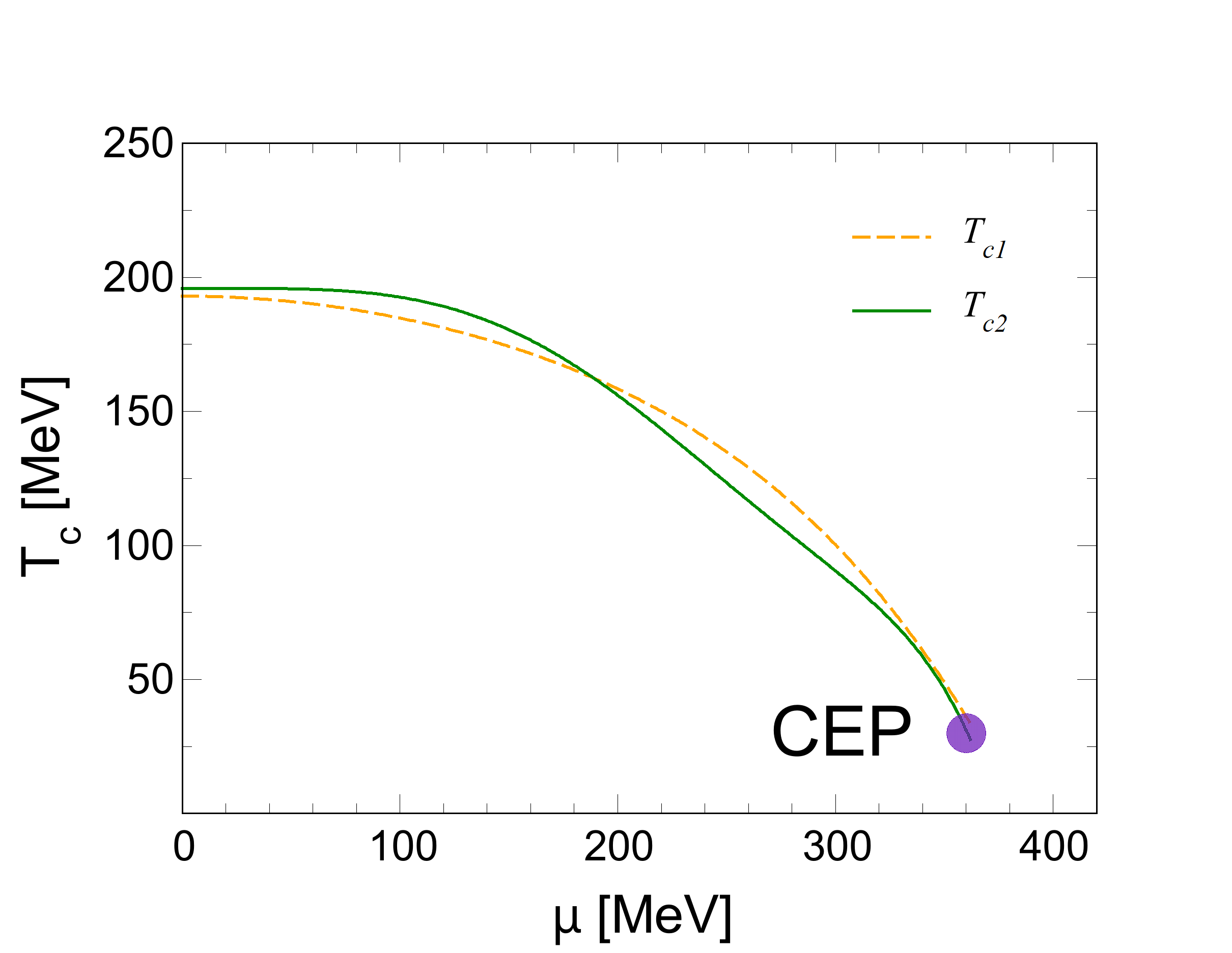
Figure 3: Critical temperatures, $T_{c1}$ and $T_{c2}$, as a function of the chemical potential. The indigo dot denotes the critical end point (CEP).

In the model at hand, as well as in full QCD, there is no real phase transition at high temperature and small chemical potential, rather only a smooth crossover. Because of this, the location of the critical temperature is ambiguous: for example, the crossover region can be identified around the temperature at which $|dM/dT|$ is maximum, or by the location of the peak of the chiral susceptibility. We define two critical temperatures:

$$T_{c1}:\leavevmode\nobreak\ \mathrm{from\leavevmode\nobreak\ the\leavevmode\nobreak\ peak\leavevmode\nobreak\ of\leavevmode\nobreak\ }\left|\frac{dM}{dT}\right|,$$ (34)

$$T_{c2}:\leavevmode\nobreak\ \mathrm{from\leavevmode\nobreak\ the\leavevmode\nobreak\ positive\leavevmode\nobreak\ peak\leavevmode\nobreak\ of\leavevmode\nobreak\ }R.$$ (35)

In particular, using $T_{c1}$ we define the crossover at a given $\mu$ by choosing the temperature at which the constituent quark mass has its maximum change. In Fig. 3 we plot $T_{c1}$ and $T_{c2}$ as a function of the chemical potential. The two lines end up and coincide at the critical endpoint, which is denoted by an indigo dot. The two critical temperatures differ for few percent at most, therefore the local maxima of $R$ in the $(T,\mu)$ plane are very close to the points at which the constituent quark mass has its maximum change which supports the idea that the peaks of $R$ do relate to the chiral crossover.

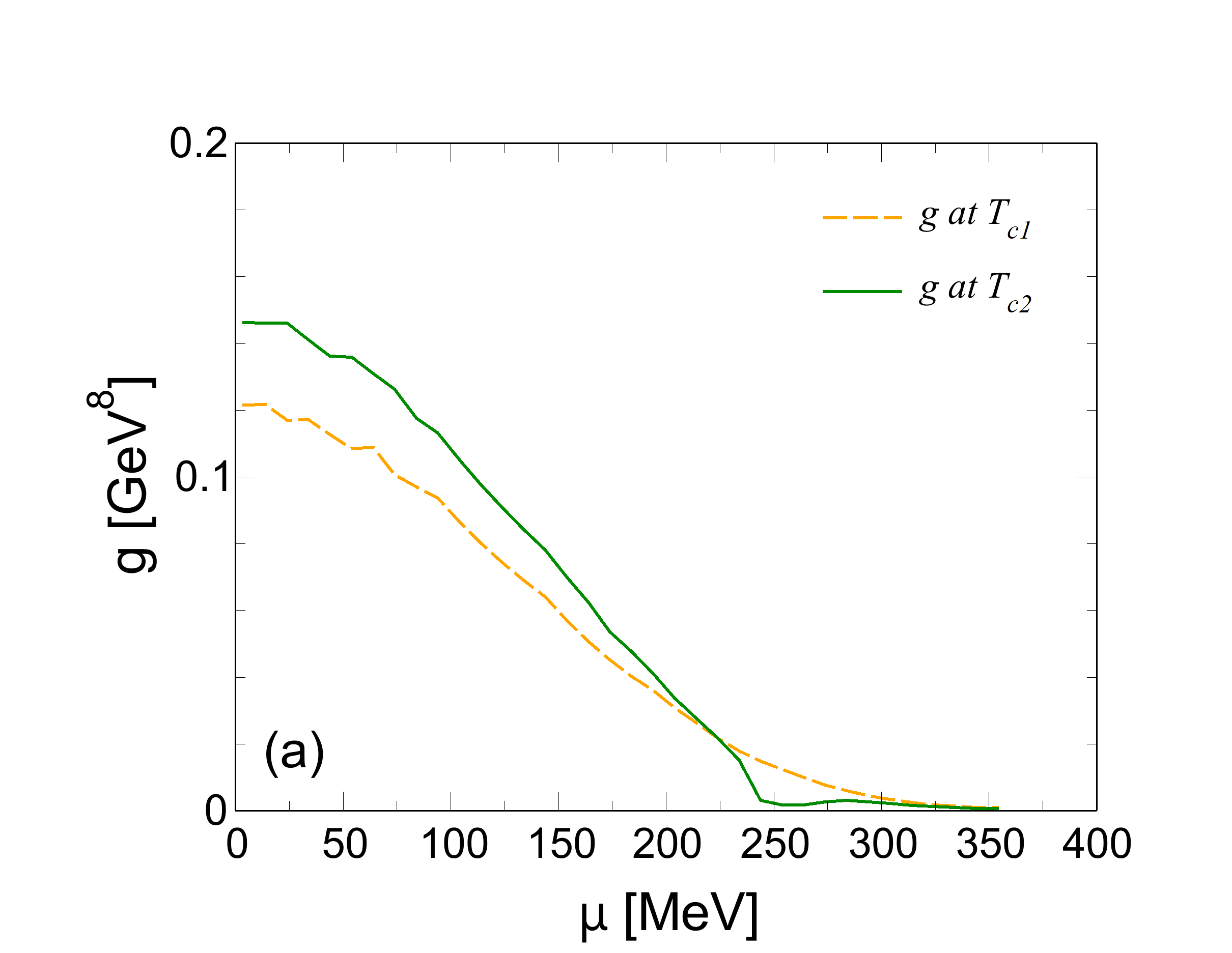
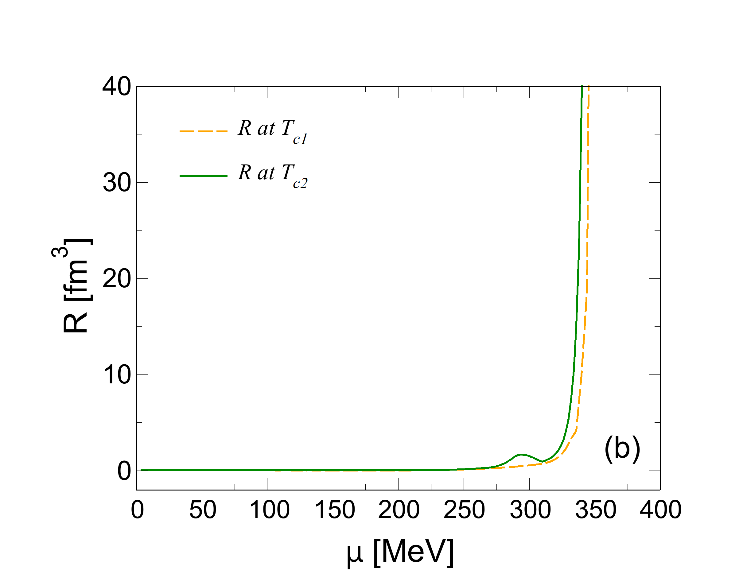
Figure 4: Panel (a). Determinant of the metric: orange dashed line corresponds to the value computed $T_{c1}$, solid green line to the value computed at $T_{c2}$. Panel (b). Thermodynamic curvature versus temperature. Color and line conventions are the same used for Panel (a).

In the panel (a) of Fig. 4 we plot the determinant of the metric, $g$, in proximity of the critical line. The orange dashed line corresponds to the value of $g$ computed at $T_{c1}$, while the solid green line denote the values of $g$ computed at $T_{c2}$. We notice that $g$ is always positive in the crossover region hence thermodynamic distance is well defined there and the system is thermodynamically stable. The mismatch between the two curves is clearly related to the definition used for the critical temperature; nevertheless, the qualitative behavior of $g$ is the same in the two cases. We also find that around the CEP the determinant is very small and eventually vanishes at the CEP, as anticipated: the vanishing of the dererminant at the CEP is expected at a second order phase transition on the base of thermodynamic stability CALLEN ; moreover, because $g=0$ at the CEP we get that $R$ diverges there, as it happens for example for the van der Waals gas geometrical:aspects ; math_santoro ; Janyszek:2 .

In the panel (b) of Fig. 4 we plot $R$ at the critical temperature. Again, we compare the result obtained using two different definitions of the critical temperature: the orange dashed line denotes $R$ computed at $T_{c1}$, while the solid green line denote the values of $R$ computed at $T_{c2}$. We notice that in both cases the qualitative behavior of $R$ is the same. In particular, the magnitude of $R$ increases when $(T,\mu)$ approach the CEP and diverges at the CEP, in agreement with the previous discussion. The divergence of $R$ at the CEP supports the idea that $|R|$ measures the correlation volume around the phase transition since the latter also diverges at the CEP Ruppeiner:1979trg .

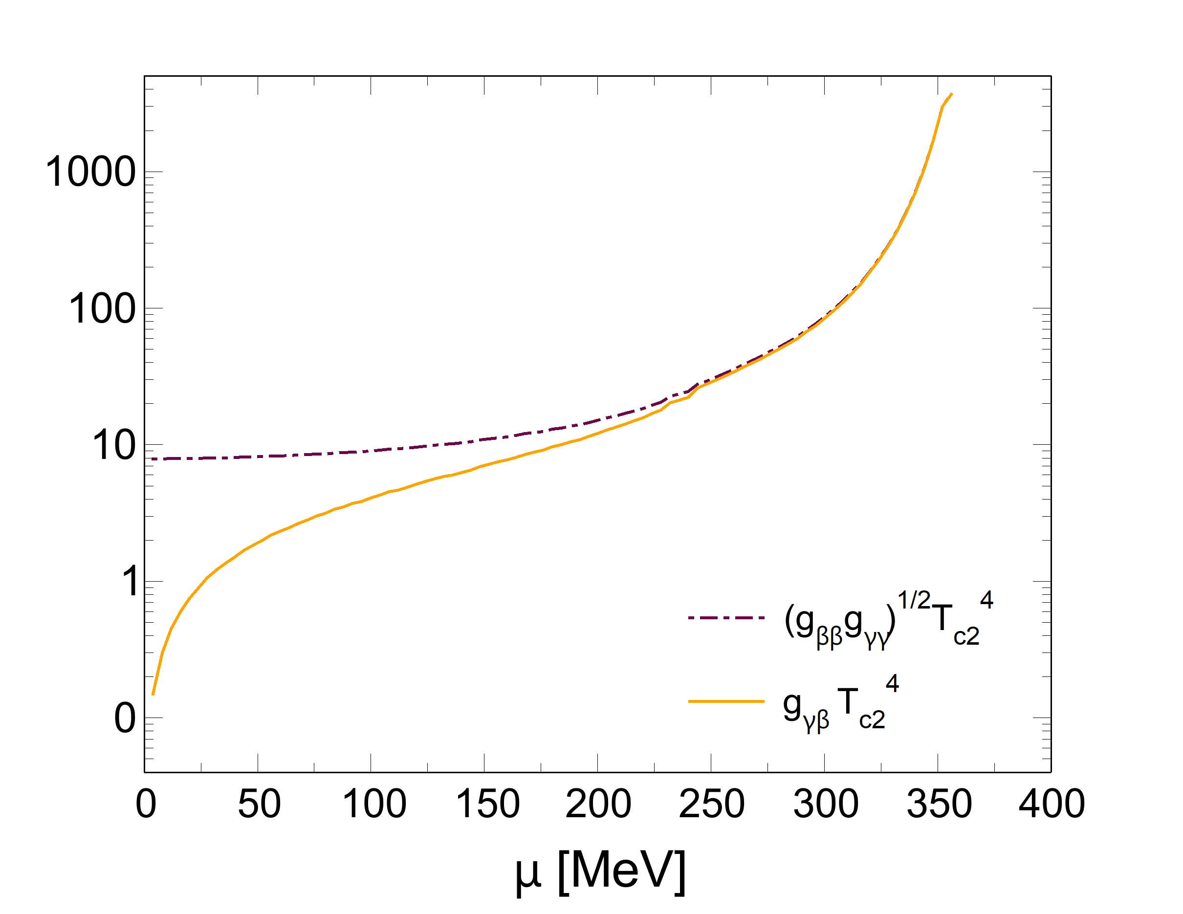
Figure 5: $T_{c2}^{4}(g_{\beta\beta}g_{\gamma\gamma})^{1/2}$ (indigo dot-dashed line) and $T_{c2}^{4}g_{\beta\gamma}$ (orange solid line) as a function of the chemical potential along $T_{c2}$.

The thermodynamic curvature diverges at the CEP because the determinant of the metric is zero there: the condition $g=0$ corresponds to thermodynamic instability and thus to a phase transition. Clearly we can write (see Section II for more details)

$$g = g_{\beta\beta}g_{\gamma\gamma}-g_{\beta\gamma}^{2}$$ (36)

$$= \left\langle(\Delta U)^{2}\right\rangle\left\langle(\Delta N)^{2}\right\rangle-\left\langle\Delta U\Delta N\right\rangle^{2},$$ (37)

where in particular $\left\langle\Delta U\Delta N\right\rangle$ corresponds to the mixed energy-baryon number fluctuation. In Fig. 5 we plot $T_{c2}^{4}(g_{\beta\beta}g_{\gamma\gamma})^{1/2}$ (indigo dot-dashed line) and $T_{c2}^{4}g_{\beta\gamma}$ (orange solid line) as a function of the chemical potential along $T_{c2}$ (for $T_{c1}$ we get similar results therefore we do not show them here). At $\mu=0$ we find $g_{\beta\gamma}=0$ thus $g>0$; as $\mu$ is increased the mixed susceptibility rapidly grows up and hits eventually $(g_{\beta\beta}g_{\gamma\gamma})^{1/2}$ leading to $g=0$ and to the divergent curvature. We conclude that the CEP (i.e. the divergent curvature) occurs in the phase diagram because the underlying microscopic interaction leads to a rapidly increasing mixed energy and baryon number fluctuation. We notice that the vanishing of $g$ is something more than getting a divergent baryon number susceptibility at the CEP: in fact, at the CEP all the matrix elements of the metric diverge, but it is the vanishing of the determinant that guarantees that $R$ diverges and thus the crossover becomes a second order phase transition. We will discuss how the mixed susceptibility is sensitive to the location of the CEP in a forthcoming article.

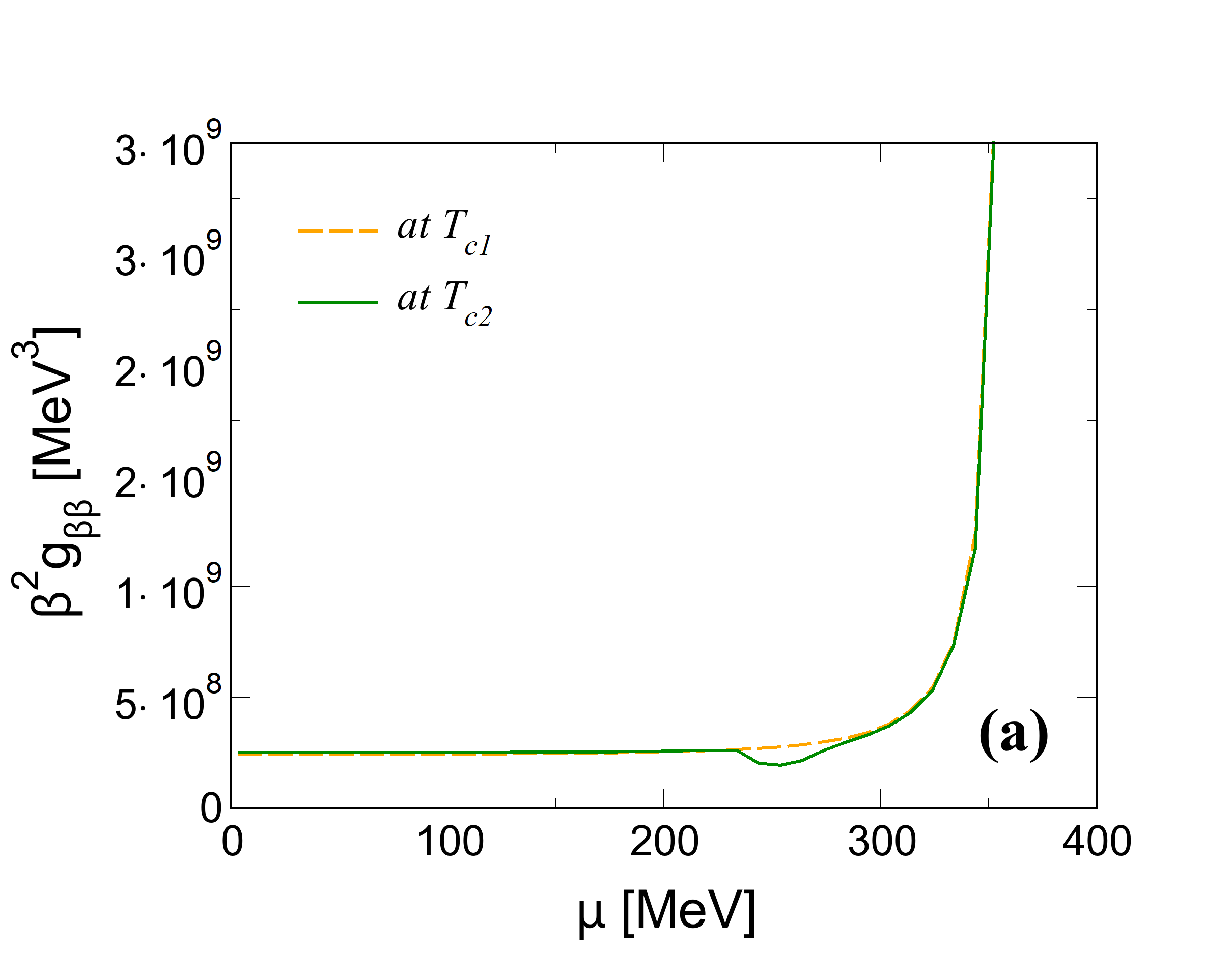
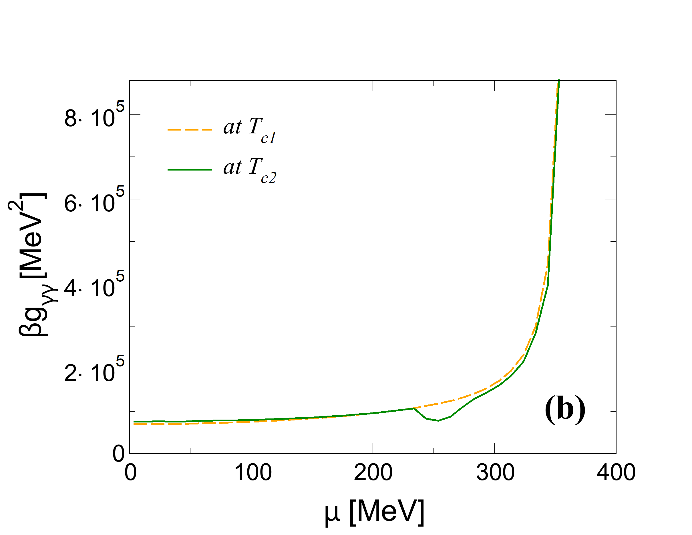
Figure 6: $\beta^{2}g_{\beta\beta}$ (panel (a)), $\beta g_{\gamma\gamma}$ (panel (b)) at the critical line. Orange dashed line corresponds to data computed at $T_{c1}$ while green solid line denote data computed at $T_{c2}$.

In Fig. 6 we plot $\beta^{2}g_{\beta\beta}$ (panel (a)) and $\beta g_{\gamma\gamma}$ (panel (b)) at the critical line. Orange dashed line corresponds to data computed at $T_{c1}$ while green solid line denote data computed at $T_{c2}$. According to Eqs. (11) and (12), $\beta^{2}g_{\beta\beta}$ and $\beta g_{\gamma\gamma}$ are proportional to the specific heat and the isothermal compressibility respectively. We notice that both quantities stay finite around the crossover at small $\mu$ but diverge as the critical endpoint is approached, in agreement with the fact that crossover becomes a second order phase transition there.

V Summary and Conclusions

We have applied the concept of thermodynamic geometry, in particular of thermodynamic curvature $R$, to the chiral crossover of Quantum Chromodynamics (QCD) at finite temperature, $T$ and finite baryon chemical potential, $\mu$. The crossover has been modeled by the renormalized Quark-Meson model (QM model) which is capable to describe the spontaneous breaking chiral symmetry. Although thermodynamic geometry has been introduced many years ago, its use for the high temperature phase of QCD has been only marginal. One of the merits of $R$ is that $|R|\propto\xi^{3}$ near a second order phase transition in three spatial dimensions, where $\xi$ corresponds to the correlation length; in QCD a crossover is expected at high temperature instead of a real second order phase transition therefore the interpretation of $R$ has to be done carefully, nevertheless it is fair to relate the peaks of $R$ to the chiral crossover. We support this idea here, albeit some detail that in our opinion deserve further studying.

We have studied $R$ for the QM model at finite $T$ and $\mu$. In the QM model the mass constituent quark mass, $M=M(T,\mu)$, is related to the quark condensate and it is computed self-consistently. We have found that for small values of $\mu$, where the model presents a very smooth crossover at finite temperature, increasing temperature results in a change of sign from negative to positive in the crossover region, as well as to a modest peak of $R$: this is similar to what has been observed in the Nambu-Jona-Lasinio model Castorina:2019jzw , and this peak appears in correspondence of the peak of $|dM/dT|$ so it is natural to identify the peak of $R$ with the chiral crossover. The change of sign of $R$ has been interpreted previously as an indicator of the attractive/repulsive nature of the microscopic interaction. However, in our model it is not clear whether this interpretation is legit because the interaction is always attractive, despite this $R$ changes sign around the chiral crossover. We think that this point deserves more attention and future studies. We have also studied several matrix elements of the metric, which are related to the isothermal compressibility and to the specific heat, as well as the curvature, at the critical line $T_{c}(\mu_{c})$, finding the divergence of these as the critical endpoint is approached. Overall, these results support the idea that although in QCD at small $\mu$ there is a smooth crossover rather than a phase transition, the thermodynamic curvature is capable to capture this crossover by developing local maxima around $T_{c}$.

We have also pointed out that due to fluctuations of both energy and baryon number in the grandcanonical ensemble, a mixed susceptibility, $\langle\Delta U\Delta N\rangle$, develops at finite $\mu$. We have shown that the CEP in the temperature and baryon chemical potential plane occurs when the determinant of the themodynamic metric vanishes: this happens $\langle\Delta U\Delta N\rangle$ grows up considerably at finite baryon chemical potential.

There are several aspects that deserve further investigations. Firstly, it is interesting to study how the repulsive vector interaction affects $R$ at finite $T$ and $\mu$: this indeed might shed some light on the connection between the attractive/repulsive nature of the interaction and the sign of $R$. To this end, it is useful to remark that effective models of QCD like the one used in this article are ideal tools to study the thermodynamic curvature, for at least two reasons. The first one is that the interaction is strong, so they allow to study quantitatively $R$ for systems that are quite far from the ideal gas or the weakly coupled system: in fact, most of the works done on $R$ in the last $\approx 40$ years hardly consider strongly coupled systems, therefore a fundamental understanding of $R$ for these thermodynamic systems is lacking. In addition to this, the microscopic interaction in these models is under control, so it is possible to study how the microscopic details affect $R$ around the phase transition. Moreover, it is of a certain interest to study $R(T,\mu)$ around the QCD chiral crossover using a Ginzburg-Landau effective potential, since this might lead to analytical expressions of the curvature and help to prove quantitatively the relation $|R|\propto\xi^{3}$ for the model at hand. Even more, it is certainly interesting to study the behavior of $R$ for higher dimensional varieties, for example enlarging the present two-dimensional space by a third direction representing isospin or magnetic field. Finally, it is well known that the QCD phase structure at large density is pretty rich: it is interesting to apply the ideas of thermodynamic curvature in this regime as well. All these interesting themes might be not shed new light on the phase structure of QCD, but we are confident that they will help to understand more about the significance of the thermodynamic geometry.

Moreover, the thermodynamic geometry allows for a natural definition of the CEP since this can be identified with the point in the $(T,\mu)$ plane where the determinant of the metric vanishes, which is equivalent to a precise relation between susceptibilities at the CEP: it will be interesting to study how the the susceptibilities at small and moderate $\mu$ are sensitive to the location of the CEP, hopefully to get information that can be tested in first principle calculations and shed light on the CEP in full QCD. We plan to report on this in a forthcoming article.

References

- (1) F. Weinhold, J. Chem. Phys. 63, 2479 (1975).
- (2) F. Weinhold, J. Chem. Phys. 63, 2484 (1975).
- (3) G. Ruppeiner, Phys. Rev. A 20, 1608 (1979).
- (4) G. Ruppeiner, Phys. Rev. A 24, 488 (1981).
- (5) G. Ruppeiner, Phys. Rev. A 27, 1116 (1983).
- (6) G. Ruppeiner, Phys. Rev. Lett. 50, 287 (1983).
- (7) G. Ruppeiner, Phys. Rev. A 31, 2688 (1983).
- (8) G. Ruppeiner, Phys. Rev. A 32, 3141 (1985).
- (9) G. Ruppeiner, Phys. Rev. A 34, 4316 (1986).
- (10) G. Ruppeiner, D. Christopher, Phys. Rev. A 41, 2200 (1990).
- (11) G. Ruppeiner, J. Chance, J. Chem. Phys. 177, 3700 (1990).
- (12) G. Ruppeiner, Phys. Rev. A 92, 3583 (1991).
- (13) G. Ruppeiner, Phys. Rev. E 47, 934 (1993).
- (14) G. Ruppeiner, Advances in Thermodynamics, Vol. 3, volume editors S. Sieniutycz and P. Salamon, series editor G. A. Mansoori, (Taylor and Francis, New York, 1990), page 129.
- (15) G. Ruppeiner, Rev. Mod. Phys. 67, 605 (1995).
- (16) G. Ruppeiner, Phys. Rev. E 57, 5135 (1998).
- (17) G. Ruppeiner, Phys. Rev. E 72, 016120 (2005).
- (18) G. Ruppeiner, Phys. Rev. D 78, 024016 (2008).
- (19) G. Ruppeiner, American Journal of Physics 78, 1170 (2010).
- (20) G. Ruppeiner, Phys. Rev. E 86, 021130 (2012).
- (21) G. Ruppeiner, A. Sahay, T. Sarkar, G. Sengupta, Phys. Rev. E 86, 052103 (2012).
- (22) G. Ruppeiner, Journal of Physics: Conference Series 410, 012138 (2013).
- (23) H. May, P. Mausbach, G. Ruppeiner, Phys. Rev. E 88, 032123 (2013).
- (24) G. Ruppeiner, Journal of Low Temperature Physics 174, 13 (2014).
- (25) G. Ruppeiner and S. Bellucci, Phys. Rev. E 91, 012116 (2015).
- (26) S. Bellucci and B. N. Tiwari, Physica A 390, 2074-2086 (2011).
- (27) H. May, P. Mausbach, G. Ruppeiner, Phys. Rev. E 91, 032141 (2015).
- (28) G. Ruppeiner, P. Mausbach, H. May, Phys. Lett. A 379, 646 (2015).
- (29) G. Ruppeiner, Journal of Low Temperature Physics 185, 246 (2016).
- (30) G. Ruppeiner, N. Dyjack, A. McAloon, and J. Stoops, J. Chem. Phys. 146, 224501 (2017).
- (31) S. Wei, Y. Liu, Phys. Rev. D 87, 044014 (2013).
- (32) B. Mirza, H. Mohammadzadeh, Phys. Rev. E 78, 021127 (2008).
- (33) B. Mirza, H. Mohammadzadeh, Phys. Rev. E 80, 011132 (2009).
- (34) P. Castorina, M. Imbrosciano, D. Lanteri, Phys. Rev. D 98, 096006 (2018).
- (35) A. Sahay, R. Jha, Phys. Rev. D 96, 126017 (2017).
- (36) H. Janyszek, R. Mrugala, J. Phys. A: Math. Gen. 23, 467-476 (1990).
- (37) H. Janyszek, J. Phys. A: Math. Gen. 23, 477-490 (1990).
- (38) H. Janyszek, R. Mrugala, Phys. Rev. A 39, 6515 (1989).
- (39) L. Diosi and B. Lukacs, Phys. Rev. A 31, 3415 (1995).
- (40) D. Brody and N. Rivier, Phys. Rev. E 51, 1006 (1995).
- (41) P. Castorina, M. Imbrosciano, D. Lanteri, Eur. Phys. J. Plus 134, 164 (2019).
- (42) P. Castorina, D. Lanteri, S. Mancani arXiv:1905.05296
- (43) M. E. Crooks, Phys. Rev. lett. 99, 100602 (2007).
- (44) M. Ruggieri, M. Tachibana and V. Greco, JHEP 1307, 165 (2013).
- (45) M. Ruggieri, L. Oliva, P. Castorina, R. Gatto and V. Greco, Phys. Lett. B 734, 255 (2014).
- (46) M. Frasca and M. Ruggieri, Phys. Rev. D 83, 094024 (2011).
- (47) V. Skokov, B. Friman, E. Nakano, K. Redlich and B.-J. Schaefer, Phys. Rev. D 82, 034029 (2010).
- (48) S. Borsanyi et al. [Wuppertal-Budapest Collaboration], JHEP 1009, 073 (2010).
- (49) S. Borsanyi, G. Endrodi, Z. Fodor, A. Jakovac, S. D. Katz, S. Krieg, C. Ratti and K. K. Szabo, JHEP 1011, 077 (2010).
- (50) M. Cheng et al., Phys. Rev. D 81, 054504 (2010).
- (51) A. Bazavov et al., Phys. Rev. D 85, 054503 (2012).
- (52) S. Borsanyi, Z. Fodor, C. Hoelbling, S. D. Katz, S. Krieg and K. K. Szabo, Phys. Lett. B 730, 99 (2014).
- (53) R. K. Pathria and P. B. Beale, Statistical Mechanics (Third Edition), Academic Press (2011).
- (54) L. D. Landau and E. M. Lifshitz, Course of Theoretical Physics, Volume 5, Butterworth-Heinemann (1980).
- (55) M. E. Peskin and D. V. Schroeder, “An Introduction to quantum field theory,” World Publishing Company (2000).
- (56) S. Weinberg, “The quantum theory of fields. Vol. 2: Modern applications,” Cambridge University Press (1996).
- (57) V. Vovchenko, D. V. Anchishkin, M. I. Gorenstein and R. V. Poberezhnyuk, Phys. Rev. C 92, no. 5, 054901 (2015).
- (58) Z. Li, Y. Chen, D. Li and M. Huang, Chin. Phys. C 42, no. 1, 013103 (2018).
- (59) Z. Li, K. Xu, X. Wang and M. Huang, Eur. Phys. J. C 79, no. 3, 245 (2019).
- (60) G. y. Shao, Z. d. Tang, X. y. Gao and W. b. He, Eur. Phys. J. C 78, no. 2, 138 (2018).
- (61) G. G. Saccheri, ”Euclides ab omni naevo vindicatus”, 1733. See also ”Girolamo Saccheri’s Euclides vindicatus”, an English translation of Saccheri’s original book by G. B. Halsted, Chicago, Open court publishing company, 1920.
- (62) E. Beltrami, ”Saggio sulla interpretazione della geometria non euclidea”, Gior. Mat. 6, 248-322 (1868).
- (63) N. Lobachevski , ”Geometrical researches on the theory of parallels” (1840), Translated from the original by George Bruce Halsted, Ann Arbor, Michigan: University of Michigan Library (1892).
- (64) B. A. Dubrovin, A. T. Fomenko and S. P. Novikov, Modern Geometry: Methods and Applications (Springer, New York, 1984).
- (65) M. Santoro and S. Preston, arXiv:math-ph/0505010.
- (66) H. B. Callen, ”Thermodynamics and Introduction to Thermostatistics 2nd edition,” John Wiley & Sons (1985).