Soft and hard X-ray dips in the light curves of $\gamma$ Cassiopeiae

Abstract

The available six archival XMM-Newton observations of the anomalous X-ray emitter $\gamma$ Cas (B0.5 IVe) have been surveyed for the presence of soft X-ray “dips" in X-ray light curves. In addition to discovering such events in the soft-band ($\leq$ 2 keV), we show that sometimes they are accompanied by minor, nearly simultaneous dips in the hard X-ray band. Herein we investigate how these occurrences can be understood in the “magnetic star-disk interaction" hypothesis proposed in the literature to explain the hard, variable X-ray emission of this Be star. In this scenario the soft X-ray dips are interpreted as transits by comparatively dense, soft X-ray-absorbing blobs that move across the lines of sight to the surface of the Be star. We find that these blobs have similar properties as the “cloudlets" responsible for migrating subfeatures in UV and optical spectral lines and therefore may be part of a common distribution of co-rotating occulters. The frequencies, amplitudes, and longevities of these dips vary widely. Additionally, the most recent spectra from 2014 July suggest that the “warm" ($kT$ $\approx$ 0.6-4 keV) plasma sources responsible for some of the soft flux are much more widely spread over the Be star’s surface than the hot plasma sites that dominate the flux at all X-ray energies. We finally call attention to a sudden drop in all X-ray energies of the 2014 light curve of $\gamma$ Cas and a similar sudden drop in a light curve of the “analog" HD 110432. We speculate that these could be related to appearances of particularly strong soft X-ray dips several hours earlier.

1 Introduction

$\gamma$ Cas (B0.5 IVe) is an enigmatic hard, variable X-ray star. Spectroscopic analysis of its emission shows that it consists of 3-4 components of optically thin thermal plasma (e.g., Smith et al., 2012a, hereafter “SLM12a”). Some 85-90% of this flux is emitted by a “hot" plasma with energy temperature $k$T $\approx$ 14 keV, an energy that cannot be attained by wind-driven shocks or infall onto the Be star. The remaining 10% or so is emitted by mainly “warm plasmas" with $kT$ of $\approx$0.6-4 keV.

$\gamma$ Cas is no longer a unique case of an active Be/X-ray star. It is the prototype, and still the brightest member, of a growing class of Be/X-ray stars. New members have been identified from cross-correlations of optical/infrared and X-ray catalogs, typically from sources distinguished by their anomalously high X-ray and infrared fluxes and colors (see e.g. Lopes de Oliveira et al., 2006; Nebot Gómez-Morán et al., 2015; Nazé & Motch, 2018). These stars have spectral types in the range of about O9.7–B1.5 and a luminosity class of IV, indicative of advanced main sequence ages. Smith et al. (2016, “SLM16”) have reviewed the X-ray findings through 2015 for this class, now numbering 20$+$ members. However, as we will see, recent observations of $\gamma$ Cas continue to reveal surprises not found in other types of X-ray emitting, massive stars.

$\gamma$ Cas itself is widely taken to be a near-critical rotator, with a rotational period P_rot of 1.21585 days (Smith et al., 2006; Smith, 2019, “S19”). It is well known to be in a wide binary (P$\approx$203.6 days) with a nearly circular orbit (Nemravová et al., 2012, SLM12a). The evolutionary status of the companion is unknown, but its mass is 0.9${\pm 0.4}$ M_⊙. Cross-correlations of International Ultraviolet Explorer (IUE) spectra have established that the contribution of the secondary to the $\gamma$ Cas  system’s UV flux is $<$0.6% (Wang et al., 2017). This limit demonstrates that the faint companion cannot produce the observed rapid UV flux variations found in the $\gamma$ Cas system, unless it is an sdOB star (e.g., Heber, 2009).

Two explanations have been put forward to explain the production of hard X-ray flux in $\gamma$ Cas and analogs of the class. The first is through accretion of disk or stellar wind onto a degenerate companion, with subsequent thermalization of the infall. Although very successful in explaining the emissions of various classes of X-ray Be binaries, there are difficulties with the accretion picture explaining them for $\gamma$ Cas stars (Motch et al., 2015, SLM16). These include the correlations between X-ray and UV fluxes in March 1996 and the changes in X-ray color accompanying variations in H$\alpha$ emission in the $\gamma$ Cas analog, HD45314 (Rauw et al., 2018).

The second explanation for hard X-ray generation is the “magnetic interaction" hypothesis. As the name implies, in this picture two magnetic field systems, one from the star and the other from its decretion disk, influence one another. The star’s magnetic system is thought to arise from the development of short-lived magnetic fields generated by subsurface convection (Cantiello et al., 2009; Cantiello & Braithwaite, 2011). The second magnetic system is a toroidal field created by a presumed global Magneto-Rotational Instability in the Be disk (Balbus & Hawley, 1991).

Hamaguchi et al. (2016, “H16") have reported time-variable, soft X-ray “dips" in X-ray color curves of $\gamma$ Cas from Suzaku data. They have proposed that X-ray active centers are powered by accretion onto the surface of a putative white dwarf (WD) companion by a dense Be wind. In their picture these centers are occasionally occulted by wind clumps as they fall onto the WD, causing absorption of soft X-rays. In this paper we explore this phenomenon in the context of the magnetic interaction picture.

2 XMM-Newton observations of $\gamma$ Cas

Launched in 1999 December 10 by the European Space Agency, XMM is an X-ray space observatory that has been in nearly continuous observation. Its European Photon Imaging Cameras (EPIC), comprised of three independent detectors (MOS1, MOS2, and pn), have maximum sensitivity in the energy range 0.3-12 keV and are used to provide images, medium resolution spectra, and relatively high time resolution light curves. In addition, two other independent instruments onboard XMM are the Reflection Grating Spectrometers (RGS1 and RGS2). Operating at low energies (0.3-2.5 keV), the RGSs provide high resolution spectra and (lower sensitivity) light curves. This work was based on archival XMM-Newton observations of $\gamma$ Cas obtained from its science archive (XSA), which were carried out at three different times (Table 1):

1. on 2004 February 5, in a a single observation with the $pn$, only among the EPIC cameras, running in the fast timing mode, and with both RGS cameras;

2. in 2010 with observations by all cameras in four visits, each separated from the next by about 2 weeks: July 7, July 24, August 2, and August 24 (investigated and denoted as 2010-1, 2010-2, 2010-3, and 2010-4, respectively, by SLM12a), and

3. on 2014 July 24, with all X-ray cameras.

Table 1: Log of XMM observations and the corresponding orbital binary phases of the $\gamma$ Cas system

Year	RJD	Duration (ks)	Obs ID	$\phi$orb
2004	53041.22	71	02012201	0.51
2010-1	55384.30	18	06516702	0.74
2010-2	55401.15	16	06516703	0.81
2010-3	55410.77	18	06526704	0.86
2010-4	55428.09	24	06516705	0.95
2014	56863.06	34	07436001	0.26

All these archival data were reduced anew and processed with SAS V17.0.0 tools by using calibration files available in 2018 December 21. The tasks epproc and rgsproc were initially applied to the EPIC and RGS data, respectively. The data processing followed the usual way applied to XMM-Newton observations, but assuming a conservative approach to avoid pile-up in the EPIC data excluding those collected within $<$ 10 arcsec from the position of $\gamma$ Cas in the images.

All spectra were binned such that each energy bin contains at least 25 counts, reducing Gaussian errors to a reasonable level. We used tools in XSPEC v12.10.1f to analyze the spectra. We compared these spectra with theoretical models by optimizing the $\chi^{2}$ criterion as fit and test statistic.

Except for the 2004 observation, for which only the XMM/pn data were available among the EPIC cameras, the pn, MOS1, and MOS2 light curves of all other observations were merged to compose their final, best quality light curves. We constructed the EPIC light curves in different energy bands, as described in the text. We followed the procedure of Lopes de Oliveira et al. (2010, “LSM10") for the 2004 XMM/pn data. These were obtained in the fast timing mode and thus have a uncertain calibration and increased noise at low energies. Therefore, we did not consider the pn data with energies below 0.8 keV for this observation, and have verified the timing analysis at low energies by investigating RGS light curves. We merged fluxes in orders 1 and 2 for both RGS1 and RGS2 to generate a light curve in the energy range of 0.8-2 keV, so as to check the behavior of $\gamma$ Cas in low energies for the 2004 observation.

Although not relevant for the purpose of this work, times were corrected to the barycenter of the solar system. In all cases we used light curves with initial time bins of 10 s. xronos v5.22 was used for exploration of light curves. Both tools, xspec and xronos are available as NASA/GSFC’s HEAsoft software v6.26.

3 Results of archival XMM observations

3.1 Light and soft/hard color curves for three XMM epochs

The XMM data were examined over various combinations of energy bands in the energy range 0.3-10 keV. The presence of certain “soft dip" (SD) features in the color ratio curves were noticed in various combinations of soft and hard energy bands; these will be discussed below. Individual soft bands are specified in the figures. The “hard" X-ray band is taken as the 2-10 keV, unless otherwise noted.

3.1.1 The 2014 light curve

Figure 1 exhibits the hard X-ray curve (2-10 keV; solid line) and a soft/hard color ratio curve (0.8-2 keV/2-10 keV) for the 2014 time series. The figure shows three probable semi-resolved soft/hard X-ray dips (“SD") in this interval. Because they are only semi-resolved, we will generally refer to them as a single aggregate feature in this paper. The central region of the aggregate may or may not be flat. This dip is flanked by a steep decrease of only about 25% of the original soft/hard energy color, followed by a similar steep rise to the initial color. The weak response in a similar hard band feature suggests that these color curve events are mainly due to soft flux variations.

An interesting aspect of the SD complex is a slight delay relative to the centroid of the associated dip in hard flux at 1.5-2.5 ks. We found this delay, visible as the small time difference between the two vertical lines to the left in the figure, to be 175${\pm 60}$ s. This value was obtained by measuring the centroids of least-squares Gaussians of the two features by means of the Interactive Data Language routine, gaussfit.pro. It merits report primarily because of similar SD delays found in 2004 data (see $\S$3.1.3).

Figure 1: Upper and lower panels exhibit the hard X-ray  and soft/hard color curves for $\gamma$ Cas  during the 2014 July 24 XMM observation. Times are rebinned to 50 s. A short vertical lines at 1.5-2.5 ks above the X-ray color curve connected to a dotted dashed line depict three marked semi-blended soft (0.8-2 keV) X-ray “dips." The dips in the hard flux and color ratio curves are enlarged in time by a factor of 2; Gaussian fits are superimposed. The right end of the horizontal dashed light connect to a “hard flux drop" during times 26.7-31.2 ks. The start time is modified from that of Smith et al. (2012a) to designate simultaneous camera operations.

A second major feature in Fig 1 is the sudden drop by $\approx$35% in the X-ray fluxes after time 25 ks, except for a likely “quasi-flare" aggregate at 32 ks. We cannot state with certainty that the drop’s presence at the end of the time series is only the beginning of a long-lasting, new flux plateau. However, it is a unique feature among the published X-ray light curves of $\gamma$ Cas.  For example, it is more than five times longer than brief, broad-band X-ray “cessations" discussed by Robinson & Smith (2000, “RSH”), Robinson et al. (2002, “RSH02”), and LSM10. We notice also in Fig. 1 that the drop in the soft energy fluxes appears to be slightly less than the hard fluxes, a point verified in our spectral analysis ($\S$3.2.2).

3.1.2 The 2010 light curves

Figure 2: The 2010-4 (August 19) light and soft/hard curves (rebinned to 50 s), where “soft" is shown over 0.8-2 keV (dashed; also called “moderately soft" in the text) and “very soft" over 0.3-1 keV (solid). Note two soft dip features with minima at 5-7 ks and 18-20 ks. Time windows W1 and W2 are depicted for separate spectral analyses. For clarity offsets in y of -10 and -8 units are given for W1 and W2 curves

.

Figure 2 exhibits a hard X-ray flux curve for 2010-4. In this case we include two soft/hard color curves, with one formed from “moderately soft" (0.8-2 keV) and a second from “very soft" (0.3-1 keV) fluxes; no corresponding hard flux drops are present. The main features of these color curves are preserved when the fluxes are taken from the RGS for comparison purposes rather than the EPIC cameras actually shown. According to the moderately soft color curve, time slices of the dips at 4.3-5.1 ks, 5.6-6.6 ks, and 17.6-18.3 ks exhibit almost flat-bottomed profiles. This is to say, the soft dips consist of unresolved and nearly resolved features. These windows will be considered separately for broader time intervals at 4.3-7 ks or 17.6-20 ks in our spectroscopic treatment ($\S$3.2.1).

SLM12a found no SDs in 2010-1 or 2010-3. However, in the 2010-2 observation they found six brief, shallow SDs (three separated by 2 ks, and three more by 1 ks). Again these were evident in the soft fluxes either from EPIC or, again for checking purposes, RGS cameras. Since there is less information in them, we will not attempt to quantify the implied column densities.

Adopting S19’s ephemeris for the Be star, the rotational phases at the start of the four observations in 2010 are 0.68, 0.54, 0.45, and 0.70. Note that the phases of 2010-1 and 2010-4 are essentially the same, i.e., there is substantial overlap of the implied visible stellar longitudes. Thus, whereas there are two SDs present in 2010-4, there are none in 2010-1. This means that the structures responsible for the soft X-ray occultations develop in less than the time interval between them, 44 days, and possibly much less. Additionally, the phase overlap between 2010-2 and 2010-3 is still sufficient to determine that none of the six SD events in 2010-2 were present in 2010-3, 9 days later. These are the first instances in which we can establish upper limits to the longevity of specific SD events.

3.1.3 The 2004 light curve

A search for soft/hard color dips within ${\pm}$1 ks of the hard flux dips in the 2004 light curve disclosed five short-lived ($\mathrel{\hbox{\hbox to0.0pt{\hbox{\lower 4.0pt\hbox{$\sim$}}\hss}\hbox{$<$}}}$1 ks) soft/hard dips, which as with the previous datasets are strongly present in the soft X-ray curves alone. The significance floor for these color events was at least 3$\sigma$, As for the events in 2014, for 2010, all five of these features were present for various combinations of hard and soft band energies, including RGS data. The soft-dips, though sharp, have soft/hard amplitudes of 20-25% relative to the hard fluxes. These dips appear to be nearly simultaneous with small hard flux dips but, like the longer-lived dip complex in the 2014 data, exhibit small lags of 180-600 s. The upper panel of Figure 3 shows the full hard flux and soft/hard color time series, while the lower panel displays enlargements of the five SD events.

Figure 3: Hard flux (upper0 and soft/hard color (lower) curves for the 2004 February 5 observation, where “soft" is taken again as 0.8-2 keV. Associated with five hard flux dips (vertical dashed lines) are brief color (SD) dips delayed by 200-500 s. Individual events are magnified below (2$\times$ in color, 5.5$\times$ in time.) Offsets in y are given for the sake of visualization

To summarize, our analysis of low resolution spectra demonstrates that SDs found in 2014, 2010-4, and 2004 are similar in general morphology but differ in details such as their amplitudes, sharpness, and longevity.

3.2 XMM/EPIC Spectra

The soft and hard X-ray light curves of $\gamma$ Cas generally show similar variations (e.g., LSM10). However, we found occasions during which flux curves for “soft" and “hard" behaviors were quite different. Also, we noted an extended “hard flux drop" (HD) in the 2014 observation. The times for the soft dips and “hard drop" in Fig. 1 are 0.8-2.2 ks and 26.7-31.2 ks, respectively. We proceeded to optimize their different behaviors by experimenting with soft and hard energy spectra with different soft-energy ranges. This step enabled us to define a convenient demarcation energy of 2 keV and thus the abutted limits of their energy ranges. In like manner we contrasted soft dip fluxes from the 2010-4 curve with fluxes from non-dip intervals.

We emphasize that it is beyond the scope of this work to proceed with a detailed spectral analysis. In the following, we will evaluate the XMM/EPIC spectra to explore the hypothesis that the variabilities reported in this paper are due to changes of the primary X-rays generated near the Be star and modified by changes in the local absorber toward the observer. To do this, we attempted to apply the model that SLM2012a determined from the 2010 observations again to the 2010-4 spectrum and also to spectra of time slices of the 2014 light curve. However, we found that the conditions during selected times of the 2014 observation varied too much to permit as good a fit as found for the 2010 data by SLM12a. This was particularly true for the description of the low energy tail, then resulting in dubious values for the emission measures of the coolest components kT₁ and kT₂.

3.2.1 Modeling the spectrum of 2010-4

Here we revisit the 2010 XMM-Newton/EPIC spectra already investigated by SLM12a under a new approach. The aim is to disentangle spectral features that characterize the soft and hard photometric dips reported in this work, which are marked in Fig. 4 as W1 (4.3-5.1, 5.6-6.6, 17.6-18.3 ks) and W2 (4.3-7, 17.6-20 ks), respectively. In this exercise we extracted three sets of spectra, each one including MOS1, MOS2, and pn spectra: the first set corresponds to data collected during W1, the second during W2, and the third, namely “nominal”, from the remaining times (precisely, $<$4 ks, 8.5-17 ks, and $>$ 20.2 ks). For the description of these spectra, we use the model presented by SLM12a that resulted from a comprehensive spectral analysis that included high resolution spectroscopy from RGS cameras.

The model then explored is that of SLM12a: $n_{H_{a}}*(T_{1}+T_{2}+T_{3}+T_{4})+n_{H_{b}}*(T_{4}+gauss)$. Our fitting procedure was to create one group in XSPEC for each sets of spectra, respectively. These were used in a simultaneous fit with a common statistics for the nine spectra. The distinction in fits for an individual group was that each of them had $n_{H_{a}}$ and normalization factors of the thermal components varying independently of the values of the other two groups. However, the temperatures ($k$T = 0.11 keV, 0.62 keV, 3.43 keV, and 13.51 keV) and $n_{H_{b}}$ values (73.7$\times$10²² cm^-2) were kept fixed to the values already obtained by SLM12a. The fit resulted in$\chi^{2}_{\nu}$ = 1.10 (degrees of freedom of 4602). In units of 10²² cm^-2, and with uncertainties of ${\pm 0.01}$ at 1$\sigma$, the results for n${}_{H_{a}}$ were 0.10, 0.23, and 0.20 for the “nominal”, W1, and W2 interval spectra, respectively. The emission measures and absorption values are presented in Table 2.

Table 2: 2010-4: best-fit spectral parameters from model $(T_{1}+T_{2}+T_{3}+T_{4})*n_{H_{a}}+(T_{4}+gauss)*n_{H_{b}}$ of Smith et al. 2012a.

State	n${}_{H_{a}}$	n${}_{H_{b}}$	EM T1 ($\times$1055 cm-3)	EM T2	EM T3	EM T4,Nha	EM T4,Nhb
	(1022 cm-2)	(1022 cm-2)	($k$T = 0.11 keV)	($k$T = 0.62)	($k$T = 3.43)	($k$T = 13.51)	($k$T = 13.51)
Nominal window	0.10${}^{+0.01}_{-0.01}$	73.71	0.14${}^{+0.04}_{-0.03}$	0.04${}^{+0.01}_{-0.01}$	0.32${}^{+0.02}_{-0.02}$	2.65${}^{+0.02}_{-0.02}$	0.90${}^{+0.14}_{-0.14}$
W1 window	0.23${}^{+0.01}_{-0.01}$	73.71	0.13${}^{+0.14}_{-0.12}$	0.04${}^{+0.01}_{-0.01}$	0.32${}^{+0.07}_{-0.07}$	2.92${}^{+0.06}_{-0.06}$	0.69${}^{+0.34}_{-0.34}$
W2 window	0.20${}^{+0.01}_{-0.01}$	73.71	0.24${}^{+0.10}_{-0.09}$	0.04${}^{+0.01}_{-0.01}$	0.36${}^{+0.05}_{-0.05}$	2.86${}^{+0.04}_{-0.04}$	1.03${}^{+0.24}_{-0.24}$

Notes: Temperatures and n${}_{H_{b}}$ from Smith et al. 2012a. Abundances solar, except $Z_{FeK\alpha}$ = 0.18$\times$$Z_{Fe,\odot}$, $Z_{N}$ = 2.33$\times$$Z_{N,\odot}$, $Z_{Ne}$ = 1.8$\times$$Z_{Ne,\odot}$.

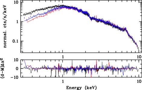
Figure 4: The 2010-4 XMM/pn spectra of $\gamma$ Cas  plotted according to the soft/hard dips and W1, W2 windows shown in Figure 2. Nominal fluxes (displayed as black) are extracted from time windows $\leq$4.0 ks, 8.5-17 ks, and $\geq$20.2 ks. W1 (in red) and W2 (in blue) refer to spectra extracted from the restrictive, and broader SD time intervals, respectively. The lower panel shows the difference between the data and the model fits (solid lines).

We note in passing for Fig. 2 that the absence of clear markers of individual SD subfeatures within the W windows, which would help define saturation levels and lifetimes of unresolved SD aggregates, suggests that our spectroscopic analysis for 2010-4 is bound to be somewhat oversimplified: our computed parameters represent some ill-defined average of possibly several events. Nonetheless, we believe our n${}_{H_{a}}$ values in Table 2 are not much different from those of any unresolved rapid events within the W windows. Coincidence or not, notice that the relatively low column densities derived for these events are roughly offset by their comparatively long durations.

3.2.2 Modeling the 2014 spectrum

As presented in $\S$3.1.1, the variability in the brightness of $\gamma$ Cas was remarkably energy-dependent in two events during 2014: a strong soft/hard flux dip early in the time series, followed by a relatively strong dip especially in the hard energy fluxes near the end. Although a detailed spectral analysis is not warranted, we have replicated the same reasoning applied to the 2010-4 spectra in $\S$3.2.1 to test the hypothesis that the color variations during the soft dip are due to changes in the local X-ray absorbers. Also, we expand the exercise to search for clues concerning the origin of the hard drop. We start by displaying XMM/EPIC spectra associated to the soft (SD; 0.8-2.2 ks) and hard (HD; 26.7-31.2 ks) dips, and a third set corresponding to a “nominal” state (all other tmes before 25 ks). For the sake of clarity, we show in Fig. 5 only the XMM/pn spectra of each window.

Departing from the approach applied to the 2010-4 set of spectra, we investigate separately the three set of EPIC windowed spectra of the 2014 observation. First, we applied the same model as for the 2010-4 observation ($\S$3.2.1) for the 2014 set of spectra representing the “nominal” state. We fixed the temperature as for the 2010-4 and allowed the $n_{H_{a}}$, $n_{H_{b}}$, and normalization of the thermal components to vary. It resulted in $n_{H_{b}}$ = 23.7${}^{+2.2}_{-1.8}$$\times$10²² cm^-2 and $\chi^{2}_{\nu}$ = 1.25 (d.o.f. = 2649). The $n_{H_{b}}$ value was kept fixed when applying the same model to the SD spectra ($\chi^{2}_{\nu}$ = 1.21; d.o.f. = 600), then to the HD spectra ($\chi^{2}_{\nu}$ = 1.06; d.o.f. = 1504). The resulting $n_{H_{a}}$ values in units of 10²² cm^-2 were 0.18$\pm$0.01, 0.87$\pm$0.02, and 0.12$\pm$0.01, for the “nominal,” SD, and HD sets of spectra, respectively. Thus, the $n_{H_{a}}$ value for the SD in 2014 is some four times larger than the maximum value we found for 2010-4. (However, note that the SD spectrum refers to the entire event, including ingress and egress times, so this column may be a lower limit.) Interestingly, the $n_{H_{a}}$ for the the HD is actually less than for the nominal fluxes. This is consistent with the very slight rise in the color in Fig. 1 compared to the level earlier in the time series.

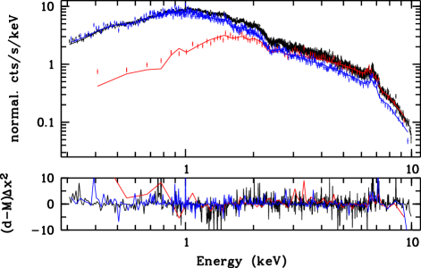
Figure 5: The 2014 XMM/pn spectra of $\gamma$ Cas  plotted according to soft X-ray dip (“SD,"in red), hard X-ray drop (blue), and “nominal flux" (black) times from Figure 1.

Notice in Fig. 4 and Fig. 5 that the “‘ultra-soft" energies ($\leq$0.8 keV) extracted from the 2014 nominal flux times and the fluxes from the W1 and W2 times (2010) no longer diverge because the spectral slopes become parallel. In fact for the 2014 data (Fig. 5) the observed fluxes at $<$0.8 keV exceed the predicted ones, even though the match is quite good for less soft fluxes at 0.8-2 keV. We discuss this behavior, also found in H16’s Suzaku spectra, in $\S$4.4.

We digress to point out that although the major thrust of this paper is to study rapid changes in X-ray absorption in $\gamma$ Cas,  i.e., $n_{H_{a}}$, our derived value of n${}_{H_{b}}$ = 23.7$\times$10²² cm^-2 is interesting in the larger context of this star’s outburst history. SLM12’s XMM 2010 observations and 2010-2011 optical continuation showed that the star had just started a Be outburst, resulting in matter being added to the disk and perhaps wind. At that time n${}_{H_{b}}$ increased over the range 36-74$\times$10²² cm^-2. Our 2014 value shows that this activity was still ongoing. By comparison, in a 2004 observation LSM10 found a $n_{H_{b}}$ of only 0.23$\times$10²² cm^-2.

4 Discussion

4.1 The context of the magnetic interaction picture

As noted in $\S$1, Cantiello et al. (2009) and Cantiello & Braithwaite (2011) have predicted that an iron-opacity convection zone is set up within the outer equatorial zone of very rapidly rotating massive stars. These authors have suggested that the convection should generate small-scale magnetic fields, the strengths and scale lengths of which are characterized by the convective velocities and cell sizes.

Moreover, the tangling of individual field lines from the stellar surface and toroidal lines from the Be disk causes stresses and ultimately their breaking and reconnections. The ensuing relaxation of the magnetic tensions proceeds as a slingshot, thereby accelerating high energy electron beams to the surface of the Be star. This description has been elaborated upon by Robinson & Smith (2000, “RS00”), Robinson et al. (2002, “RS02”), and S19.

The X-ray light curves of $\gamma$ Cas exhibit ubiquitous rapid “quasi-flares" that Smith et al. (1998a, “SRC98”) interpreted as explosive releases of beam energy in the photosphere. Such events of course are not true flares in the solar sense but rather the manifestations of thermal conversion of the beam energy and the subsequent adiabatic expansion of hot plasma, which then accumulates in a magnetically confined, overhead “canopy" of lower density. It is in fact in these canopies where most ($\sim$70%) of the hard (“basal") X-rays are released. This energy is also released as X-rays over a longer timescale as the canopy plasma cools. Empirically, the flare and basal flux temperatures are the same to within $\approx$10% (SRC98), a fact that sets important constraints for physical models.

S19 have identified the X-ray emitting canopies with co-rotating “cloudlets," observed as the Doppler motion of migrating subfeatures (msf) in UV and optical line profiles. These bodies absorb flux as they move transversely across the line of sight in front of surface activity centers (SRC98, Smith & Robinson, 1999). The msf have common timescales of appearance and inferred column densities as the basal X-ray canopies, and thus they are likely the same bodies. or at least parts of a common distribution. We reiterate that the evidence for cloudlets comes from UV and optical line variability. Therefore they must originate from the Be star.

4.2 Interpretation of the 2014 hard X-ray dip accompanying the soft dip

To discuss the X-ray dips, and beginning with the 2014 hard dip, we consider, first, that the magnetic strengths associated with the convective cells predicted by Cantiello et al. have a limit imposed by the equipartition of their magnetic and turbulent energies. Accordingly, an ensemble of active cells across the surface of the Be star will host a distribution of magnetic strengths peaking at this limit and tapering to lower values. Although most cells should have this characteristic magnetic field strength, an occasional one will host a weaker one.

As a second consideration, we return to the SRC98 picture of the generation of quasi-flares and the resulting basal flux emitted from an overhead canopy. Since the source of these fluxes is the incident electron beam, the emission measure of the flare, EM_flare, is proportional to the beam energy. However, this strict proportionality does not necessarily extend to EM_canopy as well because of nonadiabatic losses there: first as the canopy fills, and more importantly as the post-flare canopy plasma cools. The basal emission is related to the canopy’s magnetic confinement, which in turn depends on both the magnetic flux at the surface anchor footpoints and the gas-magnetic pressure equilibrium at the apex of the canopy. Indeed, the abrupt ingress/egress of the soft and hard X-ray dips associated with the canopy has sharp leading and trailing edges suggests that it is confined by an external pressure.

Turning to a possible explanation of the hard flux dip in Fig. 1, since the emission measure of the canopy, EM_canopy $\propto$ $N_{e}^{2}$ $V_{\rm canopy}$, and given that the volume is inversely proportional to the electron density, it follows that EM_canopy is simply proportional to $N_{e}$. Then, the overall hard X-ray flux contribution from all canopies above active centers on the visible disk depends mainly on the average magnetic field surrounding the canopies.

Elaborating further on this description, let us consider that whenever an electron beam impacts an surface active center which hosts a weaker than average surface field, the radius of the associated canopy, such as we will associate with any of the three SD events in Fig. 1, will become larger than others associated with stronger fields. Given its relatively low density, the EM of our designated canopy will be likewise low, the deficit having gone into more adiabatic expansion to fill a larger volume. The sum of all basal flux contributions across the visible disk will now be decreased by a small amount because of our one canopy’s reduced emission. Meanwhile, several other emitting canopies, each with an average EM, will produce greater X-ray fluxes than our designated canopy. Altogether, its weaker field will result in a reduction in the basal flux integrated across the disk.

4.3 The soft X-ray dips

4.3.1 The SDs in the XMM  light curves

In the 2014 time series each of the three semi-resolved SDs last 0.5-1 ks. We interpret their presence as being caused by absorption by one or more canopies, moving transversely in the line of sight over a small magnetic active surface region on the Be star. Since during even the core phase, the soft/hard ratio dips only by $\sim$25%, the area of the X-ray source on the star is likely smaller than the overhead occulting cloudlet. Thus, the canopy flanges outward from the active surface area projected toward the observer. H16 reached similar conclusions.

In $\S$4.1 we identified the primarily UV-absorbing “cloudlets" with structures responsible for msfs appearing across line profiles. Combining the inferred transverse velocities of 95 km s^-1 of these structures as they pass through the stellar meridian and their lifetimes of $\sim$5 ks for the largest feature occurring at 1.5 ks in Fig. 1, we find the diameter of a typical cloudlet is $\sim$5$\times$10⁵ km. This UV-based timescale is comparable to the X-ray based timescale for the strongest feature(s) occurring at 2 ks in Fig. 1. Thus, the derived diameter of a typical cloudlet becomes 3-5$\times$10⁵ km. While still small, this value is much larger than the initial size of individual quasi-flare parcels, $\sim$3-5$\times$10³ km (SRC98), on the star’s surface. RS00 showed that a high energy electron beam of this diameter directed toward the star can generate a considerable amount of X-ray energy (1.5$\times$10³² erg) upon impacting the stellar surface. This is of order 15% of the integrated energy of a flare on $\gamma$ Cas.

SRC98 gave an rough particle density estimate of 10¹¹ cm^-3 for a canopy, which we may now compare with an estimate from time delays of the SDs seen in the 2004 and 2014 light and color curves. The straightforward interpretation of the SD lags is that they represent a decay timescale of a plasma with a lower density than the initial quasi-flare volume. A decay of $\sim$300 s is expected for a hot plasma with a density of 3$\times$10¹¹ cm^-3, or just a factor of three off the earlier estimate. Although neither of these values is precise, they are determined by independent means.

4.3.2 Size comparisons for corotating occulting structures

A check on our tentative inference that so-called cloudlets, responsible for msf in optical/UV lines, are also responsible for at least some of the X-ray SDs can be made from estimates of their physical sizes. S19 estimated size of typical cloudlets as $\approx$1$\times$10⁵ km. If we adopt a time interval of 600 s separating semi-resolved SD components in Fig. 1 in terms of stellar longitude ranges of rotationally advected blobs, next use the star’s rotational period (1.21 d), radius of 10R${\rm*}$, and finally take a rotational inclination of 45^∘, we can derive a size of 2-3$\times$10⁵ km, depending on whether the active features are at a stellar latitude of 45^∘ or on the equator. Perhaps even smaller values obtain for even briefer SDs, such as suggested by the SDs in 2004 (Fig. 3). However, in such cases, fainter msf signatures in UV spectra might not be observable.

If for the X-ray canopy we take these size and electron density estimates, and assume a roughly spherical shape, a column density of about 4.5$\times$10²¹ cm^-2 results. This is within a factor of two or so of the spectroscopically derived value in $\S$3.2.2. Altogether, the physical estimates of the absorbing parameters from the X-ray and UV domains are in good agreement.

4.3.3 SDs in the context of recent literature

H16 have reported a few soft (also defined as below 2 keV) dips in a 111 ks long Suzaku observation on 2011 July 13-14. They interpreted these features as arising from absorbing structures having column densities of 2.4–8.1$\times$10²¹ cm^-2. This is similar to the $\sim$10²² cm^-2 we found for the column density responsible for the principal soft dip in Fig. 1. No simultaneous variations in the hard X-ray light curve could be found. In all, H16 identified six SD features, probably with time-symmetric profiles. In three cases their profiles were “flat-bottomed," indicating saturated absorption, in terms of optical thickness.

The duration and profile of some of the saturated dips, as well as the column density H16 derived for an occulting feature moving in front of the X-ray  source, reveals the same phenomenology as our 2014 SD event. The primary difference, crucially, between their interpretation and ours is that they consider the occulting structures to be Be wind blobs moving transversely across X-ray sites on a putative magnetic WD.

H16 rejected the idea X-ray  plasma sources could be emitted near the Be star for the stated reason that in the interaction scenario active centers must be “spread evenly" across the Be star, whereas these authors reasoned that most of the X-ray emission must arise on two centers on the X-ray-active star. However, other than as a occasional artifice, our previous papers advocating the magnetic interaction picture were not predicated on the assumption of a quasi-random spatial distribution of sources. (For example, the appearance of large variations of the basal emissions in 1996 January and March are likely due to two widely separated major active centers advecting across a rotating Be star (SRC98), at least at that time). Also, H16 attributed the major flat-bottomed dips in the Suzaku data to two major X-ray emitting centers on a magnetic dipole, This suggests a full rotational period of roughly 1.6 days, which is consistent with the 1.2 day period for $\gamma$ Cas. Thus, there is no clear contraindication of the X-ray variations being emitting from the Be star. Rather, their Dip #6 is likely a reoccurrence of Dip #1 one rotational cycle later if the emissions originate from the Be star.

Recently, Hamaguchi (2018, “H18”) has observed SD events in $\gamma$ Cas using the Neutron Star Interior Composition Explorer (NICER) satellite. These observations occurred during during 2017 June 24 and September 29, for a total duration of 57 ks, This instrument is very sensitive to soft ($\sim$1 keV) X-rays, allowing the search for more short-lived color variations. These light curves show a “rapid, consecutive [soft X-ray] dipping" that “comes and goes" even within 2 ks. These dips are similar to those we reported for the 2004 and 2010 observations.

The occurrence of the SDs distributed in phases around the binary orbit (Table 1) demonstrates that they need not occur during special orbital alignments of the primary and secondary with respect to the observer. Thus there is no evidence for a velocity vector other than transverse motion for absorbing blobs that cause the SDs.

It is now clear that the foreground occulting canopies/blobs may be either ephemeral and rendered visible sporadically over a particular activity center, or long-lived. In the latter case, lines of sight to one of them will successively intersect different surface centers that are advected across the stellar surface by rotation. Not enough events have really been recorded to establish which is the more likely case. However, from the limited number of events to date, it can be argued that some of them favor one or the other explanations at different times. In particular, very closely spaced events in Fig. 1 suggest successive activation of small regions over a closely spaced area of the star. Alternatively, the series of SDs over a time corresponding to 60% of the Be star’s rotational period (Fig. 3) implies active sites are distributed over a broad range of surface longitudes. Repeated hard/soft X-ray observations showing similar column densities for SDs spaced closely in time should further test these possibilities.

The SD events of observations of $\gamma$ Cas  recorded by H16, H18, and those observed by the XMM ($\S$3.1), suggest a picture in which major X-ray centers are not stable. This fact contradicts a picture that includes a permanent magnetic dipole, regardless of the identity of the X-ray active star. It is therefore inconsistent with the presence of a fossil field, such as would be required for most magnetic WD accretion models. Our inference of magnetic impermanence follows also from an examination of the earlier X-ray monitorings of $\gamma$ Cas. For example, although a dipole picture for the Be star could be maintained in principle from the 1996 March observations of SRC98, later observations do not bear out a continuity. Observations spaced a few days apart in 1998 showed only a trace of similar major X-ray features (RS00).

Any picture in which hard X-rays are emitted from a single magnetically active region (by necessity, small-scale and highly multipolar) must explain occasional series of apparent reoccurrences, or “flickers," of SD events. This conclusion is reinforced by the ubiquitous appearance of quasi-flares. In tallying up the shortcomings of the WD and interaction scenarios, on one hand H16’s WD scenario suffers the flaws of not accounting for stability of robust dipolar fields, and of assuming a very high mass loss rate for the Be star (see $\S$4.6). Even so, the interaction scenario relies on a complicated and unproven interplay between the presence of subsurface convective cells and (still undetected) small-scale, multipolar magnetic fields that guide high energy electron beams to the surface sporadically.

4.4 Behavior of the soft X-ray fluxes

In $\S$3.2 we discussed the 2014 and 2010-4) soft X-ray spectra and noted two unexpected results.

The first, in the spectrum for 2014 (Fig.5), there is an unexpected comparative “excess" of soft X-ray flux of the HD spectrum (once the high energy flux is renormalized to the fluxes of the NF spectrum) that is particularly evident. This is to say, during the drop phase the soft flux exhibits less of a decrease than the hard flux in Fig. 1. The most likely realization of this puzzle is that nearly all the soft flux persists fully even when a substantial fraction of the hard X-ray sources is occulted. It follows that the soft and hard flux sources are not strictly cospatial. Rather, they are more nearly outside the occulting lines of sight, and possibly distributed all around the star. Candidates for the origin of this flux are the warm plasma components $kT_{2}$ and/or $kT_{3}$ mentioned in $\S$3.2.1.

The second unexpected result in both Figs.  4 and 5 is that at the “ultra-soft" energies the slopes of the SD interval spectra became less steep, no longer diverging with spectral fluxes from the nominal flux intervals. In general, one expects that the softest fluxes should be attenuated progressively toward softer energies by photoelectric absorption. How can this result be explained? Reference to the model spectra of each of the component plasmas comprising the total spectrum of $\gamma$ Cas,  such Fig. 7 of LSM10, Fig. 5 of SLM12a, one sees that the warm plasma emissions are no longer quite so subordinate to the hot plasma emissions as they are at higher energies. If, for example, the hot plasma responsible for the hard flux disappears while residual warm plasma sites are still visible on the suface, the warm plasmas’ emissions can have a greater influence at soft energies and in particular cause a shallower spectral slope at the lowest energies. We hasten to point out that this is a speculative conclusion based on few independent spectral bins (albeit of two observations). More spectral observations during extended SD events can test this explanation.

4.5 The hard X-ray drops of $\gamma$ Cas  (and HD 110432)

Of special interest in Fig. 1 is the sustained drop in the hard X-ray curve that occurs at 25-27 ks into the observation and lasts for 5 ks of the remaining 7 ks of the observation. The soft/hard color curve is essentially constant during this duration. Such a drop has not been reported for $\gamma$ Cas.  The event cannot be confused with the very brief ($\leq$ 1 ks) “cessations" first noted by Smith et al. (1998b) and subsequent authors. Although this drop behavior is unique in the $\gamma$ Cas  record, it did remind us of a similar drop of nearly 50% in the hard X-ray flux of the $\gamma$ Cas-analog HD 110432, which was first reported by Smith et al. (2012b) and is reproduced as our Figure 6, along with the soft/“all" color curve. Here the “soft" band is taken as 0.6-2 keV and “all" as 0.6-12 keV. The drop is similarly sudden and lasts for the remaining 40 ks of the time series. As in Fig. 1 there is no accompanying change in the color curve although the drop in integrated energies is halved. the time over which the hard flux is reduced with respect to the Fig. 1 drop for $\gamma$ Cas is halved or less.

Figure 6: Upper and lower panels depict the All energies X-ray  and soft/hard color curves for HD 110432 during the XMM observation of 2007 Sep 7; “soft" refers to 0.6-2 keV fluxes. A flat-bottomed soft dip occurs at 0-13 ks. A hard dip, dropping by $\sim$50% from the nominal level before time 25 ks, occurs some 27 ks later.

There is again to be an ambiguity in attributing these events to changes in the source energy supply versus those in geometry. On one hand, there are no other observational precedents for sustained drops in the source term (impinging electron beams in the interaction scenario), although new surprises keep arising with increased observational scrutiny of these star’s high energy behavior. On the other hand, we point out that the centroid of the soft dip for $\gamma$ Cas  in Fig. 1 occurs 25 ks before the transition of the hard drop. There is a corresponding interval of 27 ks for the light and color curves of HD 110432. In both cases this interval happens to be about $\frac{1}{4}$ of the Be star’s rotational period (not precisely known). Thus, one explanation, consistent with the “pencil column" explanation for the UV continuum dip in early 1996 (S19), is that a pre-wind absorption column is responsible for the soft dip. Then, the activity center disappears with rotation over the receding limb of the Be star and approximately half the hard X-ray flux is quickly removed from our visibility. There are doubtless other explanations, and until further examples come to light we will not speculate further on the “hard drop phenomenon."

4.6 Notes on the WD accretion hypothesis

Limits on the secondary star’s mass of the $\gamma$ Cas system inferred from its mass function, as well as the optically thin, thermal spectrum, make it unlikely that a neutron star emits the X-rays. Also, limits on the contribution to UV flux rule out the secondary being a sdBO star. The secondary is either a main sequence star, or more likely if $\gamma$ Cas is a blue straggler, a white dwarf. A key difficulty for WD accretion, as noted long ago by White et al. (1982), is for the Be star to have sufficient mass loss to power the observed L_x of $\sim$10³³ erg s^-1 via WD accretion.

Fitting of asymmetric wings of UV resonance line profiles led Hammerschlag-Hensberge et al. (1980) to a mass loss estimate of 1$\times$10^-8 M_⊙ yr^-1 for $\gamma$ Cas. However, a recent Viscuous Decretion Disk model, with fitting across the near infrared, has placed the loss rate of $\gamma$ Cas at 2-2.5$\times$10^-10 M_⊙ yr^-1 (Vieira et al., 2017). This is up to three orders of magnitude below the range obtained by Lamers & Waters (1987) of up to 5$\times$10^-7 M_⊙ yr^-1), which is near the value used by H16 to justify a WD accretion picture. We also point out that the Lamers & Waters estimates were based on highly uncertain assumptions, including an extrapolation of an arbitrary wind velocity at the star’s surface as well as a large range in the assumed ionization equilibrium in the wind.

Finally, contrary to H16, there is no evidence for clumping in the $\gamma$ Cas wind on rapid timescales (e.g., Cranmer et al., 2000), as could otherwise be reasonably argued for O and B supergiants (Lépine & Moffat, 2008; Prinja & Massa, 2010). Altogether, these arguments suggest the WD accretion picture cannot be sustained from what we now believe are the wind conditions for $\gamma$ Cas.

5 Summary and Conclusions

The highlighting by Hamaguchi et al. (2016) of the soft-energy X-ray dips (SDs), accompanied by minor or no hard X-ray dips, has revealed a new phenomenon by which to study the environment of the hard X-ray production of $\gamma$ Cas. It is important to study this environment, first, to elucidate the locations and potentially the creation mechanism of the hot plasma. Second, these studies reveal a means to disambiguate the positions of the dominant “hot" plasma from the “warm" ones.

Our estimates of particle densities, column densities, and sizes of the soft X-ray absorbing “canopies" are close to independent estimates of the “cloudlets" responsible for msf in primarily UV lines. In addition, the n_H values for our ensemble of SDs exhibit a range of 0.23-0.87$\times$10²² cm^-2, which perhaps fortuitously almost perfectly matches the range 0.24-0.81$\times$10²² cm^-2 found by H16 using Suzaku data. These values have a range of a factor of about four, suggesting that the canopies responsible for them have a distribution of sizes. By comparison, these values are nearly two orders of magnitude higher than the interstellar medium column estimate of 1.45${\pm 0.3}$$\times$10²⁰ cm^-2 from the most detailed UV data (Jenkins, 2009).

Our analyses of spectra obtained from the SDs in 2014 and 2010-4 indicates that the steep drop off in slope moderates at energies below 0.7 keV. This similarity suggests that although the emission of the hot plasma at 14 keV dominates, it dominates less at these energies. The presence of warmer plasm components discussed by previous authors, which from our results appears to be spread more evenly over the star, is making its presence felt at these low energies.

We have also discovered, in agreement with the H16 and H18 studies, that the SDs can occur as more or less isolated light curve features events several hours apart (2014, 2010-2, and 2010-4) or as several brief events at seemingly random, but more closely spaced, intervals. Accumulating more statistics on the strengths and event-to-event frequencies of SD events in the future should help decide whether lines of sight to one surface center, per rotational advection, intersect to other nearby centers. In such a case a relatively large number of centers - or, that there are few centers being “turned on and off" by repeated beam injections into those few centers. Our preference at the moment is for repeated beam injections to produce most events, such as in the 2014 light curve. However, we suspect also the former case occurs sometimes, e.g., again as in the 2004 light curve. A resolution of this question may shed light on the degree and rate of change of the magnetic topology, which in turn is critical to reconciling so far unsuccessful attempts to detect complex magnetic fields by spectropolarimetric means.

Finally, we have suggested that hard X-ray drops, unaccompanied by SDs, can occur in both $\gamma$ Cas and HD 110432. More long observations of these stars should be gathered to explore the idea that these occur one-quarter of a rotational cycle after (and equally before) the appearance of a strong SD. Such a possibility would tie the existence of major activity centers to the Be star’s rotation. If this idea is not born out, an alternate explanation must be advanced to understand how much of both the soft and hard X-ray fluxes can be suddenly turned off for intervals of at least 2-3 hours.

We dedicate this paper to the memory of Mrs. Eleanor Smith.

References

- Balbus & Hawley (1991) Balbus, S. & Hawley, J. F. 1991, ApJ, 376, 214B
- Cantiello & Braithwaite (2011) Cantiello, M., & Braithwaite, J. 2011, A&A, 540A, 140C
- Cantiello et al. (2009) Cantiello, M., Langer, N., Brott, I., et al. 2009, A&A, 499, 279C
- Cranmer et al. (2000) Cranmer, S. R., Smith, M. A., & Robinson, R. D. 2000, ApJ, 537, 433C
- Hamaguchi (2018) Hamaguchi, K. 2019, in “The Gamma Cas Phenomenon in Be stars (Strasbourg, France), https://gammacas-enigma,sciencesconf.org/ (H18)
- Hamaguchi et al. (2016) Hamaguchi, K., Oskinova, L., Russell, C., et al. 2016, ApJ, 832, 140H (H16)
- Hammerschlag-Hensberge et al. (1980) Hammerschlag-Hensberge, G., van den Heuvel, E. P., Lamers, H. J., et al. A. & A. 85, 119H
- Heber (2009) Heber, U. 2009, Ann. Rev. of Astron. & Astrophys., 47, 211H
- Henrichs et al. (1983) Henrichs, H. F., Hammerschlag-Hensberge, G., Howarth, I. D., et al. 1983, ApJ, 268, 807H
- Jenkins (2009) Jenkins, E. B. 2009, ApJ, 700, 1299J
- Lamers & Waters (1987) Lamers, H. J. & Waters, L. B. 1987, A & A, 182, 80W
- Lépine & Moffat (2008) Lépine, S. & Moffat, A. F. 2008, AJ, 136, 548L
- Lopes de Oliveira et al. (2006) Lopes de Oliveira, R., Motch, C., Haberl, F., Negueruela, I., & Janot-Pacheco, E. 2006, A&A, 454, 265
- Lopes de Oliveira et al. (2010) Lopes de Oliveira, R, Smith, M. A., & Motch, C. 2010, A&A, 512, A22L (LSM10)
- Mamajek (2017) Mamajek, E. 2017, J. Dbl. Star Obsns, 13, 264M
- Motch et al. (2015) Motch, C., Lopes de Oliveira, R., & Smith, M. A. 2015, ApJ, 806, 177M
- Nazé & Motch (2018) Nazé, Y., & Motch, C. 2018, A&A, 619A, 148N
- Nazé et al. (2017) Nazé, Y., Rauw, G., & Cazoria, C. 2018, A&A, 602L, 5N
- Nebot Gómez-Morán et al. (2015) Nebot Gómez-Morán, A., Motch, C., Pineau, F.-X., et al. 2015, MNRAS, 452, 884N0
- Nemravová et al. (2012) Nemravová, J., Harmanec, P., Koubska, P., et al. 2012, A&A, 537, 59-69N
- Postnov et al. (2017) Postnov, K., Oskinova, L., & Torrej́on, J. M. 2017, arXiv:2017.00336v1
- Prinja & Massa (2010) Prinja, R. K., & Massa, D. L. 2010, A&A, 521,L55P
- Rauw et al. (2018) Rauw, G., Nazé, Y., Smith, M. A., et al. 2018, A&Ak 615A, 44R
- Robinson & Smith (2000) Robinson, R. D., & Smith, M. A. 2000, ApJ, 540, 474R (RS00)
- Robinson et al. (2002) Robinson, R. D., Smith, M. A., & Henry, G. 2002, ApJ, 575, 435R (RSH02)
- Smith (2006) Smith, M. A. 2006, A&A, 615, 215S
- Smith (2019) Smith, M. A. 2019, PASP, 131, 4201S (S19)
- Smith et al. (2004) Smith, M. A., Cohen, D. H., Gu, M. G., et al. 2004, ApJ,600, 972S (S04)
- Smith et al. (2006) Smith, M. A., Henry, G. W., & Vishniac, E. 2006, ApJ, 647, 1375
- Smith et al. (2012a) Smith, M. A., Lopes de Oliveira, R., & Motch, C., et al. 2012, A&A, 540, A53S (SLM12a)
- Smith et al. (2012b) Smith, M. A., Lopes de Oliveira, R., & Motch, C. 2012b, ApJ, 755, 64S (SLM12b)
- Smith et al. (2016) Smith, M. A., Lopes de Oliveira, R., & Motch, C., 2016, AdSpR, 58, 782S (SLM16)
- Smith et al. (2017) Smith, M. A., Lopes de Oliveira, R., & Motch, C., 2017, MNRAS, 469, 1502S
- Smith & Robinson (1999) Smith, M. A., & Robinson, R. D. 1999, ApJ, 517, 866S ; (SR99)
- Smith et al. (1998a) Smith, M. A., Robinson, R. D., Corbet, R. H. 1998a, ApJ, 503, 877S (SRC98)
- Smith et al. (1998b) Smith, M. A., Robinson, R. D., Hatzes, A. P.. 1998b, ApJ, 508, 945S )
- Vieira et al. (2017) Vieira, R., Carciofi, A., Bjorkman, J., et al. 2017, MNRAS, 464, 3071V
- Wang et al. (2017) Wang L., Gies, D. R., & Peters, G. J. 2017, ApJ, 843, 60W
- White et al. (1982) White, N. E., Swank, J. H., Holt, S. S., et al. 1982, ApJ, 263, 277W