Abstract

In this paper, we study a Bianchi type -I model of universe filled with barotropic and dark energy(DE) type fluids. The present values of cosmological parameters such as Hubble constant $H_{0}$, barotropic, DE and anisotropy energy parameters $(\Omega_{m})_{0}$, $(\Omega_{de})_{0}$ and $(\Omega_{\sigma})_{0}$ and Equation of State(EoS) parameter for DE ($\omega_{de}$) are statistically estimated in two ways by taking 38 point data set of Hubble parameter H(z) and 581 point data set of distance modulus of supernovae in the range $0\leq z\leq 1.414$. It is found that the results agree with the Planck result [P.A.R. Ade, et al., Astron. Astrophys. 594 A14 (2016)] and more latest result obtained by Amirhashchi and Amirhashchi [H. Amirhashchi and S. Amirhashchi, arXiv:1811.05400v4 (2019)]. Various physical properties such as age of the universe, deceleration parameter etc have also been investigated.

Key Words: Dark Energy; Accelerating universe; Bianchi type-I space-time.

1 Introduction;

SN Ia observations [1]$-$[4] confirm the fact that our observable universe is accelerating at present. This surprising discovery is a break through in the field of observational cosmology and had lead to a presence of an unknown dark energy(DE) fluid that opposes gravitational attraction. It is a common perception that DE has positive energy density and negative pressure so that it creates acceleration in the universe. Although, it violate the strong energy condition (SEC), yet provides an elegant description of transition of universe from deceleration to cosmic acceleration (Caldwell et al.[5]). In the framework of general relativity, the dynamics of dark energy could be understand through it’s equation of state parameter which is defined as $\omega^{(de)}=p^{(de)}/\rho^{(de)}$ where $p^{(de)}$ and $\rho^{(de)}$ are the pressure and energy density of dark energy component respectively. It is well known that $\omega^{(de)}=-1$ represents the standard $\Lambda$CDM model of universe.

After CMB experiment, It has been now confirmed that the matter distribution inside the present universe is on whole isotropic but early universe had not such smooth picture i.e. it was anisotropic near the singularity point. So, one has to assume anisotropy in the background of evolving process of current universe. Off late, spatially homogeneous and anisotropic cosmology had been a matter of interest to the cosmologists. Recently, Akarsu et al. [6] have constructed Bianchi type I model (BT-I) as natural extension of the standard $\Lambda$CDM model. Amirhashchi and Amirhashchi [7] have investigated three DE models for flat and curved FLRW and BT- I space times and put constraints on cosmological parameters using Gaussian processes and MCMC method. In other papers [8, 9], they developed BT-I Universe with Type Ia Supernova and H(z) Data and have probed DE in the scope of BT-I space time. Mishra et al. [10] investigated the role of anisotropic components on the DE and the dynamics of the universe in Bianchi-V string cosmological model. In another papers [11, 12], they have also discussed Bulk viscous embedded BT- I dark energy models. Recently Rashid et al. [13] have also developed anisotropic DE model. More information and references regarding BT-I DE models can be found in Goswami et al. [14]$-$[20]. Some important applications of BT-I cosmological models in the framework of general relativity and modified theories of gravitation are given in Refs. [21, 22, 23, 24, 25, 26, 27].

In this paper, we study a BT -I model of universe filled with barotropic and DE perfect fluids. The present values of cosmological parameters such as Hubble constant $H_{0}$, barotropic, DE and anisotropy energy parameters $(\Omega_{m})_{0}$, $(\Omega_{de})_{0}$ and $(\Omega_{\sigma})_{0}$ and Equation of State(EoS) parameter for DE $\omega_{de}$ are statistically estimated in two ways by taking 38 point data set of Hubble parameter H(z) and 581 point data set of distance modulus of supernovas in the range $0\leq z\leq 1.414$. It is found that the results agrees with the Planck findings [28] and more latest results due to Amirhashchi and Amirhashchi [29]. The contents of the paper in brief are as follows : In section 2, we have described the field equation for BT- I universe. In section 3 and 5, Hubble and energy parameters were estimated in the two ways on the basis of 38 data set of H(z) and a distance modulus data set of 581 Supernovas. In section 4, luminosity distance, distance modulus and apparent magnitude in our model have been formulated. In section 6, Various physical properties such as age of the universe, deceleration parameter etc have also been investigated. Finally the concluding remarks are presented in section 7.

2 Field equations for Bianchi Type I Universe

We consider a general BT- I metric

$$ds^{2}=dt^{2}-a^{2}dx^{2}-b^{2}dy^{2}-c^{2}dz^{2},$$ (1)

where a, b and c are scale factors along spatial directions and it depend on time only.

Let the universe be filled with two type of fluids: one is barotropic and other creating dark energy. We assume that suffix m stands for matter and de for dark energy.
The energy momentum tensor(EMT) has two components i.e. $T_{ij}=T_{ij}(m)+T_{ij}(de)$. The followings are the EMTs of the contents of the universe, $T_{ij}(m)=\left(\rho_{m}+p_{m}\right)u_{i}u_{j}-p_{m}g_{ij}$ and $T_{ij}(de)=\left(\rho_{de}+p_{de}\right)u_{i}u_{j}-p_{de}g_{ij}$. For co-moving co-ordinates $u^{\alpha}=0;\;\;\alpha=1,2~{}\&~{}3$, where $g_{ij}u^{i}u^{j}=1$. The Einstein field equations are

$$R_{ij}-\frac{1}{2}Rg_{ij}=-8\pi GT_{ij},$$ (2)

where we have taken velocity of light as unity. The field equation (2) in terms of line element (1) and EMTs described above are solved as follows.[See [14] for details]
$a^{2}=bc$, $b=ad$, $c=ad^{-1}$, $2\frac{a_{44}}{a}+\frac{a^{2}_{4}}{a^{2}}+(\frac{d_{4}}{d})^{2}=-8\pi G(p_{de}+p_{m})$, $\frac{a^{2}_{4}}{a^{2}}-(\frac{d_{4}}{d})^{2}=8\pi G(\rho_{m}+\rho_{de})$ and $(\frac{d_{4}}{d})_{4}+3\frac{a_{4}d_{4}}{ad}=0$, which on integration gives $\frac{d_{4}}{d}=\frac{k}{a^{3}}$, where k is an arbitrary constant of integration. The Hubble’s parameter H in this model is as follows $H=\frac{1}{3}(\frac{a_{4}}{a}+\frac{b_{4}}{b}+\frac{c_{4}}{c})=\frac{a_{4}}{a}$. Finally we get following field equations for BT-I anisotropic universe

$$2\frac{a_{44}}{a}+\frac{a^{2}_{4}}{a^{2}}=-8\pi G(p_{de}+p_{m}+p_{\sigma})$$ (3)

$$H^{2}=\frac{a^{2}_{4}}{a^{2}}=\frac{8\pi G}{3}(\rho_{m}+\rho_{de}+\rho_{\sigma})$$ (4)

where we have considered anisotropy terms $\frac{d_{4}}{d}$ appearing in the field equations as anisotropy energy represented by suffix $\sigma$ whose pressure and density are given by

$$p_{\sigma}=\rho_{\sigma}=\frac{k^{2}}{8\pi Ga^{6}}.$$ (5)

During course of its evolution, the universe had gone through a stage where matter density and pressure were equal. That stage is called stiff matter filled universe. So we can say that anisotropy energy behaves like stiff matter. The energy conservation law for our model is as follows $T_{j}^{ij}=\dot{\rho}+3H(p+\rho)=0$, where $\rho=\rho_{m}+\rho_{de}+\rho_{\sigma}$ and $p=p_{m}+p_{de}+p_{\sigma}$. We see that $\dot{\rho_{\sigma}}+3H(p_{\sigma}+\rho_{\sigma})=0$ holds separately. So we have $\frac{d}{dt}{(\rho_{m}+\rho_{de})}+3H(p_{m}+p_{de}+\rho_{m}+\rho_{de})=0.$ We assume that dark energies does not interact with barotropic matter , so that they are conserved simultaneously i.e. $(\rho_{m})_{4}+3H(p_{m}+\rho_{m})=0$ and $(\rho_{de})_{4}+3H(p_{de}+\rho_{de})=0$. The equations of states are as follows $p_{m}=\omega_{m}\rho_{m}$, where $\omega_{m}$ are constants. For matter in form of radiation $\omega_{m}=\frac{1}{3},\rho_{m}\varpropto a^{-4}.$ Present universe is dust filled for which $\omega_{m}=0,\rho_{m}\varpropto a^{-3}.$ Now we use the following relation between scale factor a and red shift z, $\frac{a_{0}}{a}=1+z$. This gives $\rho_{\sigma}=(\rho_{\sigma})_{0}[\frac{a_{0}}{a}]^{6}=(\rho_{\sigma})_{0}(1+z)^{6}.$ Similarly $\rho_{de}=(\rho_{de})_{0}[\frac{a_{0}}{a}]^{3(1+\omega_{de})}=(\rho_{de})_{0}(1+z)^{3(1+\omega_{de})},$ where $\omega_{de}$ is equation of state parameter for dark energy which is considered as constant for present epoch. We take $p_{m}=0$ for dust filled universe and define following energy parameters $\Omega_{m}=\frac{\rho_{m}}{\rho_{c}},~{}~{}\Omega_{de}=\frac{\rho_{de}}{\rho_{c}},~{}~{}\&~{}~{}\Omega_{\sigma}=\frac{\rho_{\sigma}}{\rho_{c}}$, where $\rho_{c}=\frac{3H^{2}}{8\pi G}$.

The field equations (3) and (4) now take following form

$$(2q-1)H^{2}=3H^{2}_{0}\left(\omega_{de}(\Omega_{de})_{0}(1+z)^{3(1+\omega_{de})}+(\Omega_{\sigma})_{0}(1+z)^{6}\right)$$ (6)

and

$$H^{2}=H^{2}_{0}\left((\Omega_{m})_{0}(1+z)^{3}+(\Omega_{de})_{0}(1+z)^{3(1+\omega_{de})}+(\Omega_{\sigma})_{0}(1+z)^{6}\right)$$ (7)

where $q=\frac{\ddot{a}}{aH^{2}}$ is deceleration parameter(DP).

The relationship amongst the energy parameters are obtained from Eq.(7) as

$$(\Omega_{m})_{0}+(\Omega_{de})_{0}+(\Omega_{\sigma})_{0}=1$$

3 Hubble and energy parameters based on 38 data set of H(z)

So many astrophysical scientists [31] $-$ [35] estimated Hubble constant $H_{0}$, as $72\pm 8,~{}~{}69.7^{+4.9}_{-5.0},~{}~{}71\pm 2.5,~{}~{}70.4^{+1.3}_{-1.4},~{}~{}73.8\pm 2.4$ and $~{}~{}67\pm 3.2$ in the unit $kms^{-1}Mpc^{-1}$ respectively, with the help of Hubble Space Telescope (HST) ,Cepheid variable observations, gravitational lensing , WMAP seven-year data and WMAP results with Gaussian priors , infrared camera and galactic cluster data’s respectively. One may refers to Kumar [36], Sharma et al. [37] and Yadav et al. [38] for detail. We consider a observed data set of 38 Hubble parameter Hob(i) in Gyr^-1 unit with standard deviations $\sigma(i)$ for different red shifts. These were imported from Farook at el [30]. For corresponding theoretical value of H(z), we use Eq.(7), in which $H_{0},(\Omega_{m})_{0},(\Omega_{\sigma})_{0}$ and $\omega_{de}$ are unknown. It is desired to estimate values of these parameters statistically by getting Chi square given by

$$\chi^{2}[H_{0},(\Omega_{m})_{0},\omega_{de}]=\sum_{i=1}^{i=38}[(Hth(i)-Hob(i))^{2}/\sigma(i)^{2}],$$ (8)

where Hth (i)’s are theoretical values of Hubble parameter as per Eq.(7) and $\sigma(i)$’s are errors in the observed values of H(z).

We take ($0.066\leq H_{0}\leq 0.076$) , ($0.1\leq(\Omega_{m})_{0}\leq 0.5$) and EoS parameter $\omega_{de}$ in the range ( -1.3,  -0.8). As at present anisotropy is very mere, we take $(\Omega_{\sigma})_{0}$ = 0.0002. It is found that $\chi^{2}$= 33.22 i.e. 87.43 % is minimum for $H_{0}=0.068~{}Gyr^{-1}$ = 66.6 Km/sec/Mpc , $(\Omega_{m})_{0}$ =0.26 , $\omega_{de}$ = -0.83. and $(\Omega_{de})_{0}$ = 0.7398. Now we present a error bar graph as figure 1 which have 38 observational Hubble data (OHD) points (left panel) and H(z) + BAO (right panel) with possible errors as bars and a curve representing corresponding theoretical value of H(z) given by Eq(7). We also note that the solid black line represent the best fit curve of derived model and dashed blue and green lines represent the corresponding $\Lambda$CDM model ($\omega^{(de)}=-1$) respectively.

We have taken $H_{0},(\Omega_{m})_{0}$, $(\Omega_{\sigma})_{0}$ and $(\Omega_{de})_{0}$ as estimated statistically on the basis of minimum $\chi^{2}$. Figure 2 represents 1$\sigma$, 2$\sigma$ Confidence regions in the ($\Omega_{m},\omega_{de}$) plane. Inside these regions red ellipse shows our estimated values. These figures show that observed and theoretical values are close to each other.

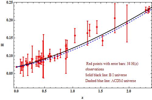
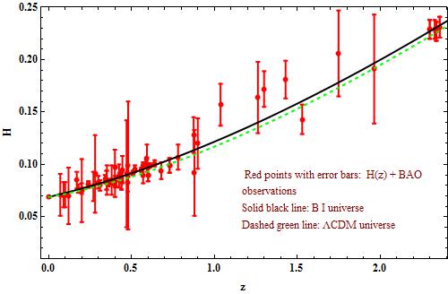
Figure 1: Hubble paprmeter $-$ red shift error bar plot with 38 OHD points (left panel) and with H(z) + BAO (right panel) for $H_{0}=0.068~{}Gyr^{-1}$ = 66.6 km/s/Mpc, $(\Omega_{m})_{0}$ =0.26, $\omega_{de}$ = -0.83 and $(\Omega_{de})_{0}$ = 0.7398.

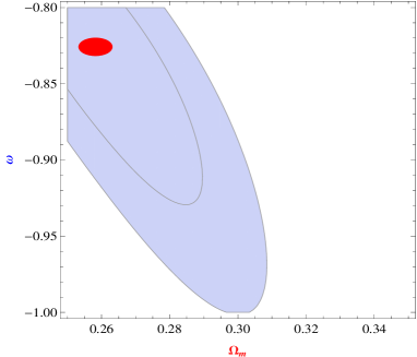
Figure 2: The likelihood contours at 1$\sigma$, 2$\sigma$ Confidence regions in $\Omega_{m}-\omega$ plane by bounding our model with 38 OHD points. Here $\omega_{de}$ is constant and it is taken as $\omega_{de}=\omega$.

4 Luminosity Distance, Distance modulus and Apparent magnitude in our model

In our earlier work [14, 15] for B-I universe, Luminosity distance $D_{L}$, Distance modulus $\mu$ and Apparent magnitude $m_{b}$ of any distant luminous object are obtained as $D_{L}=\frac{c(1+z)}{H_{0}}\int^{z}_{0}\frac{dz}{h(z)}$, $\mu=M-m_{b}=5log_{10}\left(\frac{D_{L}}{Mpc}\right)+25$ and $m_{b}=16.08+5log_{10}\left[\frac{1+z}{.026}\int^{z}_{0}\frac{dz}{h(z)}\right]$ where $h(z)=\frac{H(z)}{H_{0}}.$ There fore in the present model, these physical quantities are given as

$$D_{L}=\frac{(1+z)}{H_{0}}\int^{z}_{0}\frac{dz}{\sqrt{(\Omega_{m})_{0}(1+z)^{3}+(\Omega_{de})_{0}(1+z)^{3(1+\omega_{de})}+(\Omega_{\sigma})_{0}(1+z)^{6}}},$$ (9)

$$\mu=25+5log_{10}\left(\frac{(1+z)}{H_{0}}\int^{z}_{0}\frac{dz}{\sqrt{(\Omega_{m})_{0}(1+z)^{3}+(\Omega_{de})_{0}(1+z)^{3(1+\omega_{de})}+(\Omega_{\sigma})_{0}(1+z)^{6}}}\right)$$ (10)

and

$$m_{b}=16.08+5log_{10}(\frac{1+z}{.026}\int^{z}_{0}\frac{dz}{\sqrt{(\Omega_{m})_{0}(1+z)^{3}+(\Omega_{de})_{0}(1+z)^{3(1+\omega_{de})}+(\Omega_{\sigma})_{0}(1+z)^{6}}})$$ (11)

5 Hubble and energy parameters based on a distance modulus data set of 581 Supernovas

We consider a observed data set of distance modulus of 581 Supernovas with standard deviations  $\sigma SN1a(i)$ for different red shifts in the range $z\leq 1.414$. These were imported from Pantheon compilation [39]. For corresponding theoretical value of $\mu_{th}$, we use Eq.(10), in which $H_{0},(\Omega_{m})_{0},(\Omega_{\sigma})_{0}$ and $\omega_{de}$ are unknown. It is desired to estimate values of these parameters statistically by getting Chi square given by

$$\chi^{2}((\Omega_{m})_{0},(\Omega_{\sigma})_{0},\omega_{de})=\sum_{i=1}^{LengthSN1aData}\frac{\mu_{th}((\Omega_{m})_{0},(\Omega_{\sigma})_{0},\omega_{de})(i)-\mu_{obs}(i))^{2}}{\sigma SN1a(i)^{2}}$$ (12)

We take ($0.066\leq H_{0}\leq 0.076$) , ($0.1\leq(\Omega_{m})_{0}\leq 0.5$) and EoS parameter ($-1.3\leq\omega_{de}\leq-0.8$). Like as before, we take $(\Omega_{\sigma})_{0}$ = 0.0002. It is found that $\chi^{2}$= 562.227 i.e. 96.7$\%$ is minimum for $H_{0}$ = 70.0097, $(\Omega_{m})_{0}$ = 0.279 and $\omega_{de}$ = -1.00654. Now we present a error bar graph as figure 3 which has 581 data points with possible errors as bars and a curve representing corresponding theoretical value of $\mu(z)$ given by Eq(10). In figure 3, the solid black line represents the best fit curve of the model under consideration while dashed blue line corresponds to the $\Lambda$CDM model ($\omega^{(de)}=-1$). We have taken $H_{0},(\Omega_{m})_{0}$, $(\Omega_{\sigma})_{0}$ and $(\Omega_{de})_{0}$ as estimated statistically on the basis of minimum $\chi^{2}$. Figure(4) represents 1$\sigma$, 2$\sigma$ Confidence regions in the ($\Omega_{m},\omega_{de}$) plane. Inside these regions red ellipse shows our estimated values. These figures show that observed and theoretical values are close to each other.

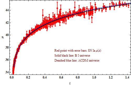
Figure 3: Distance modulus ($\mu$) $-$ red shift error bar plot for $H_{0}$ = 70.0097, $(\Omega_{m})_{0}$ = 0.279, $(\Omega_{de})_{0}$ = 0.7208 and $\omega_{de}$ = -1.00654.

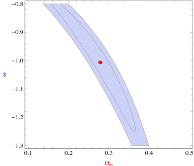
Figure 4: 1$\sigma$, 2$\sigma$ Confidence regions and our estimated point inside the red ellipse in $\Omega_{m}-\omega$ plane by bounding our model with 581 SN Ia data. Here $\omega_{de}$ is constant and it is taken as $\omega_{de}=\omega$.

6 Present age of the universe

We obtained the present age of universe as follows

$$t=\intop_{0}^{t}dt=\intop_{0}^{a}\frac{da}{aH}=\intop_{0}^{z}\frac{dz}{(1+z)H}$$

This implies that

$$t_{0}=\lim_{x\rightarrow\infty}{\int_{0}^{x}\frac{dz}{H_{0}(1+z)\sqrt{(}(\Omega_{m})_{0}(1+z)^{3}+(\Omega_{de})_{0}(1+z)^{3(1+\omega_{de})}+(\Omega_{\sigma})_{0}(1+z)^{6})}}.$$ (13)

We see that $t_{0}\rightarrow 0.95296H_{0}^{-1}$ for high red shifts of order $10^{5}$, where we have taken $H_{0}$ = 70.0097, $(\Omega_{m})_{0}$ = 0.279 and $\omega_{de}$ = -1.00654. Now $H_{0}^{-1}=13.9976~{}Gyrs$, so the present age of universe comes to $t_{0}=13.339~{}Gyrs$ for our model. If we calculate $t_{0}$ on the basis of our results $H_{0}=0.068~{}Gyr^{-1}$ = 66.6 Km/sec/Mpc , $(\Omega_{m})_{0}$ =0.26 , $\omega_{de}$ = -0.83. and $(\Omega_{de})_{0}$ = 0.7398 as per 38 pt.Hubble parameter estimation, we get age of the universe as $t_{0}=13.7711~{}Gyrs$. The empirical value of present age of the universe is $t_{0}=13.73_{-.17}^{+.13}$ as per WMAP data[40]. Thus present age of universe obtained by us is very close to observed one especially with respect to 38 OHD. Hubble parameter estimation. The figure 5 describes variation of time with red shift.

Figure 5: Red shift z versus time t plot for $H_{0}$ = 70.0097, $(\Omega_{m})_{0}$ = 0.279 and $\omega_{de}$ = -1.00654.

6.1 Deceleration Parameter

The deceleration parameter(DP) is obtained from Eqs.(6) and (7) as

$$2q=1+3\frac{\omega_{de}(\Omega_{de})_{0}(1+z)^{3(1+\omega_{de})}-\frac{1}{3}(\Omega_{\sigma})_{0}(1+z)^{6}}{\sqrt{(\Omega_{m})_{0}(1+z)^{3}+(\Omega_{\sigma})_{0}(1+z)^{6}+(\Omega_{de})_{0}(1+z)^{3(1+\omega_{de})}}}.$$ (14)

It’s present value is given as  $2(q)_{0}=1+3\omega_{de}(\Omega_{de})_{0}-(\Omega_{\sigma})_{0}$.

In absence of dark energy, our model represent an decelerating universe. Dark energy has negative pressure ($\omega_{de}<0$), so it makes the universe accelerating. For $H_{0}$ = 70.0097, $(\Omega_{m})_{0}$ = 0.279 and $\omega_{de}$ = -1.00654, the present value of DP is obtained as $(q)_{0}=-0.58837$. The present value of DP on the basis of our results $H_{0}=0.068~{}Gyr^{-}1$ , $(\Omega_{m})_{0}$ =0.26 , $\omega_{de}$ = -0.83 and $(\Omega_{de})_{0}$ =0.7398 as per 38 points. Hubble parameter estimation comes out to be equal to $(q)_{0}$= -0.421335. The following figure(6) shows how deceleration parameter q varies over red shift z. It is interesting to see that there are two transition red shift in this model $z_{t}=1.448$ and $z_{t}=4.18$. This means that our universe had gone two times though the accelerating phase. Duration of present phase is $0\leq z\leq 1.448$ and in the past it was $z\geq 4.18$. This shows that structure formation era is $1.448\leq z\leq 4.18$ and inflation might have taken place at $z\geq 4.18$. Figure(6) describes the whole evolution of the universe. It covers the main three phases of the universe, Inflation, structure formation and the present accelerating phase.

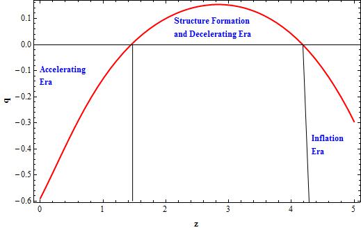
Figure 6: Deceleration parameter q over red shift z for $H_{0}$ = 70.0097, $(\Omega_{m})_{0}$ = 0.279 and $\omega_{de}$ = -1.00654.

6.2 Particle Horizon

Let us consider a light ray form a source along x-direction. Proper distance of the source will be $a_{0}x$. Let we are receiving light signal at certain time $t_{0}$. It might have transmitted in the past at certain time say $t_{p}$ from the source, then proper distance of the source form us will be given by $r=a_{0}\int_{t_{p}}^{t_{0}}\frac{dt}{a(t)}$.

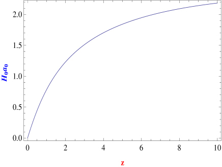
Figure 7: Red shift z versus proper distance plot for $H_{0}$ = 70.0097, $(\Omega_{m})_{0}$ = 0.279 and $\omega_{de}$ = -1.00654.

The Particle Horizon $R_{P}$ is defined as the $\lim_{t_{p}\rightarrow 0}a_{0}{\int_{t_{p}}^{t_{0}}\frac{dt}{a(t)}}=\lim_{z\rightarrow\infty}\int_{0}^{z}\frac{dz}{H(z)}$

$\therefore$

$$R_{P}=\lim_{x\rightarrow\infty}{\int_{0}^{x}\frac{dz}{H_{0}\sqrt{(}(\Omega_{m})_{0}(1+z)^{3}+(\Omega_{de})_{0}(1+z)^{3(1+\omega_{de})}+(\Omega_{\sigma})_{0}(1+z)^{6})}}.$$ (15)

We see that $R_{P}\rightarrow 2.43419H_{0}^{-1}$ for high red shift of order $10^{5}$, where we have taken $H_{0}$ = 70.0097, $(\Omega_{m})_{0}$ = 0.279 and $\omega_{de}$ = -1.00654. The value of $R_{P}$ on the basis of our results $H_{0}=0.068~{}Gyr^{-1}$ , $(\Omega_{m})_{0}$ =0.26 , $\omega_{de}$ = -0.83 and $(\Omega_{de})_{0}$ =0.7398 as per 38 OHD. Hubble parameter estimation comes out to be equal to $R_{P}\rightarrow 2.48215H_{0}^{-1}$. For FLRW model it is given as $R_{P}\sim\frac{2}{H_{0}}$.

The figure 7 describes variation of proper distance with red shift.

7 Conclusion

In this paper, we have investigated the two fluid scenario in Bianchi type I space-time. It is worth to mention that in the literature, two fluid interacting dark energy models in BT-I space-time are available [41, 42, 43]. But the mechanism for solving of field equations in present model is altogether different from the mechanism used in Refs. [41, 42, 43]. We also estimate the present values of cosmological parameters of derived model by using 38 OHD points and 581 SN Ia data. We summaries our finding with the help of the following table. We have also displayed observational data’s due to Planck for the purpose of comparison. Figure 6 of the our work is very interesting. It describes the whole evolution of the universe from it’s beginning to present epoch. It covers the main three phases of the universe, Inflation, structure formation and the current accelerating phase.

Cosmological	Values as	Values as	Planck
Parameters	per 38 OHD	per 581 SN Ia	results
at present
$(\Omega_{de})_{0}$	0.7398	0.7208	0.6911
$(\Omega_{m})_{0}$	0.26	0.279	0.3089
$(\Omega_{\sigma})_{0}$	0.0002	0.0002	0
$\omega_{de}$	-0.83	-1.00654	-1.019
$H_{0}$	66.6	70.0097	67.74
$Age~{}t_{0}$	13.7711	13.339 Gyrs	13.799
$R_{P}$	2.48215$H_{0}^{-1}$	2.43419 $H_{0}^{-1}$	—
$(q)_{0}$	-0.421335	-0.58837	—

We also quote the latest results due to Amirhashchi and Amirhashchi [29] $H_{0}=69.9\pm 1.7,(\Omega_{m})_{0}=0.279^{+0.014}_{-0.016},(\Omega_{de})_{0}=0.721^{+0:016}_{-0.014}$ and $z_{t}=0.707\pm 0.034$.

References

- [1] S. Perlmutter et al., Bull. Am. Astron. Soc., 29, 1351(1997), arXiv:astro-ph/9812473 [Supernova Cosmology Project Collaboration].
- [2] Perlmutter, S. et al., Nature, 391, 51(1998).
- [3] Perlmutter, S. et al., Astrophys. J., 517, 5(1999).
- [4] A.G. Riess et al., Astron. J., 116, 1009(1998), arXiv:astro-ph/9805201[Supernova Search Team collaboration].
- [5] R. R. Caldwell, W. Knowp, L. Parker and D. A. T. Vanzella, Phys. Rev. D 73, 023513 (2006).
- [6] O. Akarsu, Suresh Kumar, Shivani Sharma and Luigi Tedesco, Phys. Rev D, 100, 023532 (2019); arXiv:1905.06949v1 [astro-ph.CO].
- [7] Hassan Amirhashchi, Soroush Amirhashchi, arXiv: 1802.04251v4 [astro-ph.CO] (2019).
- [8] Hassan Amirhashchi, Soroush Amirhashchi, Phys. Rev D, 99, 02316 (2018); arXiv:1803.08447v2 [astro-ph.CO].
- [9] Hassan Amirhashchi, Phys. Rev. D, 97, 063515 (2018); arXiv:1712.02072v2 [astro-ph.CO].
- [10] B. Mishra, S.K. Tripathy, Pratik P. Ray, Astrophys.Space Sci., 363,86( 2018), arXiv:1701.08632 [physics-gen-ph].
- [11] B.Mishra, Pratik P. Ray, R. Myrzakulov, Euro. Phys. Journal C, 79,34, (2019), arXiv:1801.01029v2[gr-qc].
- [12] B. Mishra, S.K.Tripathi, Mod. Phys. A , 30, 1550175(2015).
- [13] Rashid Zia, Umesh Kumar Sharma, Dinesh Chandra Maurya,.New Astronomy, 72 ,83(2019).
- [14] A. K. Yadav et al., Euro. Phy. J. Plus., 127, 127(2012).
- [15] G. K. Goswami, M. Mishra, A. K. Yadav, Int. J. Theor. Phys. 54, 315 (2015).
- [16] G. K. Goswami, A. K. Yadav, R. N. Dewangan and A. Pradhan, Astrophys. Space Sci. 361, 47 (2016).
- [17] G. K. Goswami, R. N. Dewangan, A. K. Yadav, Astrophys. Space Sci. 361,119 (2016) .
- [18] G. K. Goswami, A. K. Yadav, R. N. Dewangan, Int. J. Theor. Phys. 55, 4651(2016).
- [19] G. K. Goswami, R. N. Dewangan, A. K. Yadav, Gravitation & Cosmology 22, 388 (2016).
- [20] U. K. Sharma, G. K. Goswami, A. Pradhan, Gravitation and Cosmology, 24,191 (2018).
- [21] S. Kumar, C. P. Singh, Astriphys. Space Sc, 312, 57 (2007).
- [22] C. P. Singh, S. Kumar, Int. J. Mod. Phys. A, 23, 813 (2008).
- [23] C. P. Singh, S. Kumar, Int.J.Theor.Phys., 47, 3171 (2008).
- [24] O. Akarsu, C. B. Killinc, Gen. Relativ. Gravit., 42, 119 (2010).
- [25] A. K. Yadav, Braz. J. Phys., 49, 262 (2019).
- [26] L. K. Sharma, A. K. Yadav, P. K. Sahoo, B. K. Singh, Results in Phys., 10, 738 (2018).
- [27] A. K. Yadav, V. Bhardwaj, P. K. Sahoo, Mod. Phys. Lett. A, 34, 1950145 (2019).
- [28] P.A.R. Ade, et al. [Planck Collaboration], Astron. Astrophys.,594,A14 (2016).
- [29] H. Amirhashchi and S. Amirhashchi, arXiv:1811.05400v4 (2019).
- [30] O. Farooq, et al., Astrophys. J., 835, 26 (2017).
- [31] W L Freedman et al, Astrophys. Journ., 553, 47 (2001).
- [32] S H Suyu et al, Astrophys. Jour., 711, 201 (2010).
- [33] N. Jarosik et al, Astrophys. Journ. Suppl., 192,14 (2010).
- [34] A G Riess et al, Astrophys. Journ., 730, 119 (2011).
- [35] F Beutler et al, Mon. Not. R. Astron. Soc., 416, 3017 (2011).
- [36] S Kumar, Mon. Not. Astron. Soc., 422, 2532 (2012).
- [37] L. K. Sharma, B. K. Singh and A. K. Yadav, arXiv:1907.03552 [Physics.gen-ph] (2019)
- [38] A. K. Yadav, N. Singla, M. K. Gupta and G. K. Goswami, arXiv:1908.04735 [gr-qc] (2019)
- [39] D. M. Scolnic, Astrophys. J., 859, 101(2018).
- [40] G. Hinshaw et.al., arXiv:1212.5226 [astro-ph.CO](2012).
- [41] S. Kumar, C. P. Singh, Gen. Relativ. Grav. 43, 1427 (2011)
- [42] A. K. Yadav and B. Saha, Astrophys. Space Sc. 337, 759 (2012)
- [43] A. K. Yadav, Astrophys. Space Sc. 361, 276 (2016)