Magnetization plateau of the $S=2$ antiferromagnetic Heisenberg chain with anisotropies

Abstract

We investigate the $S=2$ antiferromagnetic quantum spin chain with the exchange and single-ion anisotropies in a magnetic field, using the numerical exact diagonalization of finite-size clusters and the level spectroscopy analysis. It is found that a magnetization plateau possibly appears at a half of the saturation magnetization for some suitable anisotropy parameters. The level spectroscopy analysis indicates that the 1/2 magnetization plateau is formed by two different mechanisms, depending on the anisotropy parameters. The phase diagram of the 1/2 plateau states and some typical magnetization curves are also presented. In addition the biquadratic interaction is revealed to enhance the plateau induced by the Haldane mechanism.

I INTRODUCTION

Since Haldane predicted the spin excitation gap of the integer-spin antiferromagnetic Heisenberg chain,haldane1 ; haldane2 the spin gap based on some topological nature has attracted a lot of interest. The existence of the Haldane gap was justified by many numerical studies. botet ; nightingale ; sakai1 ; white ; todo ; nakano1 ; nakano2 ; wang Affleck, Kennedy, Lieb and Tasaki proposed a well-understandable picture of the spin gap formation, so-called the valence bond solid.aklt1 ; aklt2 The single-ion anisotropy $D$ tends to suppress the valence bond solid picture. When the anisotropy $D$ increases, a quantum phase transition occurs from the Haldane phase to the large-D phase where the topological nature disappears.sakai2 ; hida Recently Gu and WenGuWen and Pollmann et al.pollmann1 ; pollmann2 introduced the concept of symmetry protected topological (SPT) phase to the quantum spin chain. Based on their argument, the Haldane phase of $S=1$ chain is this SPT phase, while not in the case of $S=2$. On the other hand, the intermediate-$D$ phase even of $S=2$ chain predicted by Oshikawaoshikawa1 should correspond to the SPT phase. Unfortunately, early density matrix renormalization group calculation on the $S=2$ antiferromagnetic Heisenberg chain with the exchange anisotropy $\lambda$ and the single-ion one $D$ could not discover the intermediate-$D$ phase. schollwoeck1 ; schollwoeck2 ; schollwoeck3 However, our recent study on the same $S=2$ model using the numerical exact diagonalization of finite-size clusters and the level spectroscopy analysis successfully detected the intermediate-$D$ phase. tonegawa1 ; okamoto1 ; okamoto2 ; okamoto3 ; okamoto4 Since this phase appears only at a quite tiny regionkjall ; okamoto4 of the anisotropy parameter space, it would be difficult to discover it for some realistic materials. As another possibility to discover the SPT phase of the $S=2$ chain, we consider the magnetization process of the system. Since Oshikawa, Yamanaka and Affleckoya discussed the magnetization plateau as the field induced Haldane gap, this problem has been investigated very extensively. Particularly the 1/3 magnetization plateau of $S=3/2$ chain was revealed to appear for sufficiently large $D$, by the numerical exact diagonalization study.sakai3 In addition the level spectroscopy analysiskitazawa indicated that the intermediate-$D$ plateau phase, which corresponds to the SPT phase based on the VBS mechanism, as well as the large-$D$ plateau phase. Similar phenomena are expected to occur at half the saturation magnetization of the $S=2$ chain. In this paper, we consider the 1/2 magnetization state of the $S=2$ antiferromagnetic Heisenberg chain with the exchange and single-ion anisotropies using the numerical exact diagonalization of finite-size clusters and the level spectroscopy analysis, to discover the SPT phase, which corresponds to the intermediate-$D$ phase.

II MODEL

Now we examine the magnetization process of the $S=2$ antiferromagnetic Heisenberg chain with the exchange and single-ion anisotropies, denoted by $\lambda$ and $D$, respectively. The Hamiltonian is given by

$${\cal H} ={\cal H}_{0}+{\cal H}_{Z},$$ (2)

$${\cal H}_{0} =\sum_{j=1}^{L}\left[S_{j}^{x}S_{j+1}^{x}+S_{j}^{y}S_{j+1}^{y}+\lambda S_{j}^{z}S_{j+1}^{z}\right]$$

$$+D\sum_{j=1}^{L}(S_{j}^{z})^{2},$$

$${\cal H}_{Z} =-H\sum_{j=1}^{L}S_{j}^{z}.$$ (3)

The exchange interaction constant is set to be unity as the unit of energy. For $L$-site systems, the lowest energy of ${\cal H}_{0}$ in the subspace where $\sum_{j}S_{j}^{z}=M$, is denoted as $E(L,M)$. The reduced magnetization $m$ is defined as $m=M/M_{\rm s}$, where $M_{\rm s}$ denotes the saturation of the magnetization, namely $M_{\rm s}=LS$ for the spin-$S$ system. $E(L,M)$ is calculated by the Lanczos algorithm under the periodic boundary condition ($\mbox{\boldmath$S$}_{L+1}=\mbox{\boldmath$S$}_{1}$) and the twisted boundary condition ($S^{x,y}_{L+1}=-S^{x.y}_{1},S^{z}_{L+1}=S^{z}_{1}$), up to $L=12$. Both boundary conditions are necessary for the level spectroscopy analysis.

III MAGNETIZATION PLATEAU

Here we consider the state at $m=1/2$ in the magnetization process of the system (2) at $T=0$. In this state the magnetization per unit cell is $M/L$=1. Thus Oshikawa, Yamanaka and Affleck’s theoremoya suggests that the magnetization plateau possibly occurs without the spontaneous breaking of the translational symmetry, because $S-M/L={\rm integer}$. If we consider the $S=2$ object as a composite spin consisting of four $S=1/2$’s, the 1/2 magnetization plateau is expected to appear due to two different mechanisms, as shown in Fig. 1. Namely one is (a) Haldane mechanism (a singlet dimer lies on each bond), and the other is (b) large-$D$ mechanism (the energy gap is open between the states $|S^{z}=1\rangle$ and $|S^{z}=2\rangle$ at each site due to the large $D$). The 1/2 magnetization plateaux based on the two mechanisms are called the Haldane plateau and the large-$D$ plateau, respectively in this paper. Following Pollmann et al.,pollmann1 ; pollmann2 the SPT phase exists if any one of the following three global symmetries is satisfied: (i) the dihedral group of $\pi$ rotations about the $x$, $y$, and $z$ axes, (ii) the time-reversal symmetry $S_{j}^{\mu}\to-S_{j}^{\mu}$, and (iii) the space inversion symmetry with respect to a bond. It is easy to see that our Hamiltonian satisfies (iii), but neither of (i) and (ii). Since the Tomonaga-Luttinger liquid phase is also possible, the $m=1/2$ state is expected to include the three phases; the Haldane plateau, the large-$D$ plateau and the gapless (plateauless) TLL phases.

Figure 1: Two different mechanisms of the 1/2 magnetization plateau; (a) Haldane mechanism and (b) large-$D$ mechanism.

IV LEVEL SPECTROSCOPY ANALYSIS

In order to distinguish these three phases, the level spectroscopy analysis kitazawa is one of the best methods. According to this analysis, we should compare the following three energy gaps;

$$\Delta_{2}={E(L,M-2)+E(L,M+2)-2E(L,M)\over 2},$$ (4)

$$\Delta_{\rm TBC+}=E_{\rm TBC+}(L,M)-E(L,M),$$ (5)

$$\Delta_{\rm TBC-}=E_{\rm TBC-}(L,M)-E(L,M),$$ (6)

where $E_{\rm TBC+}(L,M)$ ($E_{\rm TBC-}(L,M)$) is the energy of the lowest state with the even parity (odd parity) with respect to the space inversion at the twisted bond under the twisted boundary condition, and other energies are under the periodic boundary condition. The level spectroscopy method indicates that the smallest gap among these three gaps for $M=L=M_{\rm s}/2$ determines the phase at $m=1/2$. $\Delta_{2}$, $\Delta_{\rm TBC+}$ and $\Delta_{\rm TBC-}$ correspond to the TLL, large-$D$-plateau and Haldane-plateau phases, respectively. The use of $\Delta_{{\rm TBC}\pm}$ directly reflects the above-mentioned (iii) of the condition for the existence of the SPT phase.okamoto2 The $D$ dependence of the three gaps calculated for $L=8$, 10 and 12 is plotted for $\lambda=1.0$ in Fig. 2. It suggests that at the isotropic point ($\lambda$, $D$)=(1.0, 0.0) the system is in the TLL phase and increasing $D$ gives rise to a quantum phase transition to the large-$D$ plateau phase. The phase boundary is given by the cross point between $\Delta_{2}$ and $\Delta_{\rm TBC+}$. The system size dependence of the boundary is predicted to proportional to $1/L^{2}$, which is justified in Fig. 3. It indicates that the size correction of $D_{\rm c}$ is almost proportional to $1/L^{2}$, at least for $L=$8, 10, 12. Thus we estimate the phase boundary in the thermodynamic limit as $D_{\rm c}=1.635\pm 0.001$, fitting $1/L^{2}$ to the data for $L=$8, 10, 12. Unfortunately, the Haldane plateau phase does not appear for $\lambda=1.0$, different from $S=3/2$ chain.kitazawa

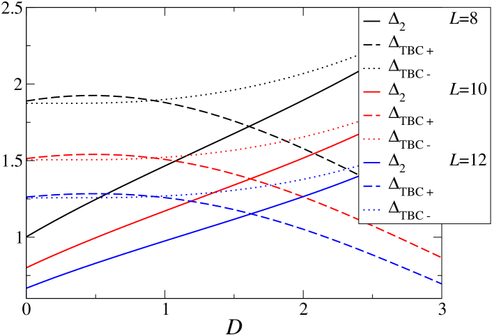
Figure 2: Level spectroscopy analysis for $\lambda=1.0$. Solid, dashed and dotted lines are for $\Delta_{2}$, $\Delta_{\rm TBC+}$ and $\Delta_{\rm TBC-}$, respectively. Black, red and blue lines are for $L=$ 8, 10 and 12, respectively.

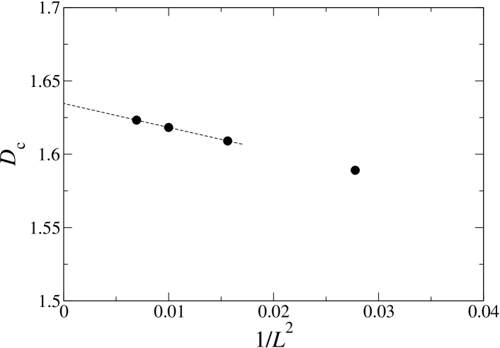
Figure 3: Extrapolation of the critical value of $D$ between the TLL and large-$D$ plateau phases to the thermodynamic limit for $\lambda=1.0$. As the $L$ dependence of $D_{c}$ for the largest three system sizes is well fitted to $1/L^{2}$, $D_{c}$ in the thermodynamic limit is estimated by the least square method.

Next, the $D$ dependence of the three gaps is plotted for $\lambda=2.0$ in Fig. 4. In this case the Haldane-plateau phase appears between the TLL and large-$D$-plateau phases. The phase boundaries $D_{\rm c1}$ between TLL and Haldane phases and $D_{\rm c2}$ between Haldane and large-$D$ phases in the thermodynamic limit are estimated as $D_{\rm c1}=0.702\pm 0.001$ and $D_{\rm c2}=1.633\pm 0.001$, using the same fitting of $1/L^{2}$.

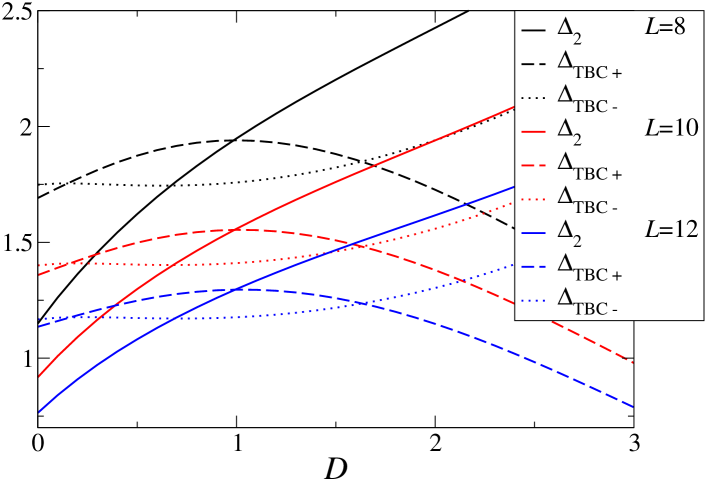
Figure 4: Level spectroscopy analysis for $\lambda=2.0$. Solid, dashed and dotted lines are for $\Delta_{2}$, $\Delta_{\rm TBC+}$ and $\Delta_{\rm TBC-}$, respectively. Black, red and blue lines are for $L=$ 8, 10 and 12, respectively.

The phase diagram on the $\lambda$-$D$ plane is shown in Fig. 5. It suggests that a tricritical point appears about ($\lambda$, $D$)=(1.55, 1.30). The Haldane-plateau phase would correspond to the SPT phase. Thus it should be called the symmetry protected topological plateau. This SPT phase appears in much wider region than that in the ground state phase diagram at $m=0$. Then the possibility of experimental discovery of the SPT phase for some real materials of the $S=2$ antiferromagnetic chain would be extended.

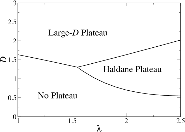
Figure 5: Phase diagram of the 1/2 magnetization state resulting from the level spectroscopy analysis. It includes the two plateau phases due to the Haldane and large-D mechanisms.

V MAGNETIZATION CURVES

Toward the experimental discovery of the 1/2 magnetization plateau, it would be useful to obtain the theoretical magnetization curve for some typical anisotropy parameters. In order to give the magnetization curve in the thermodynamic limit $L\rightarrow\infty$ using the numerical diagonalization results, we perform different extrapolation methods in the gapless and gapped cases. The magnetic fields $H_{-}(m)$ and $H_{+}(m)$ are defined as follows:

$$E(L,M)-E(L,M-1)\to H_{-}(m)\quad(L\to\infty),$$ (7)

$$E(L,M+1)-E(L,M)\to H_{+}(m)\quad(L\to\infty),$$ (8)

where the size $L$ is varied with fixed $m=M/M_{\rm s}$. If the system is gapless at $m$, the conformal field theory predicts that the size correction is proportional to $1/L$ and $H_{-}(m)$ coincides to $H_{+}(m)$.sakai4 ; sakai5 It is justified by Fig. 6, where $E(L,M)-E(L,M-1)$ and $E(L,M+1)-E(L,M)$ are plotted versus $1/L$ for $\lambda=1.0$ and $D=2.0$. It suggests that the system is gapless at $m\not=1/2$. The gapless feature at $m=0$ is consistent with the phase diagram of the previous work.tonegawa1 For these magnetization, we can estimate $H(m)$ in the thermodynamic limit, using the following extrapolation form

$${1\over 2}[E(L,M+1)-E(L,M-1)]\to H(m)+O(1/L^{2}).$$ (9)

On the other hand, if the system has a gap at $m$, namely the magnetization plateau is open, $H_{-}(m)$ does not coincides to $H_{+}(m)$ and $H_{+}(m)-H_{-}(m)$ corresponds to the plateau width. In such a case we assume the system is gapped at $m$ and use the Shanks transformationshanks ; barber to estimate $H_{-}(m)$ and ${}_{+}(m)$. The Shanks transformation applied for a sequence {$P_{L}$} is defined as the form

$$P^{\prime}_{L}={{P_{L-2}P_{L+2}-P_{L}^{2}}\over{P_{L-2}+P_{L+2}-2P_{L}}}.$$ (10)

As the above level spectroscopy analysis predicts that the 1/2 magnetization plateau appears for $\lambda=1.0$ and $D$=2.0, we use the method to estimate $H_{-}(m)$ and $H_{+}(m)$ at $m=1/2$. The Shanks transformation is applied for the sequence $E(L,M)-E(L,M-1)$ twice as shown in Table 1.

Table 1: Result of the Shanks transformation applied for the sequence $E(L,M)-E(L,M-1)$ twice.

$L$	$P_{L}$	$P_{L}^{\prime}$	$P_{L}^{\prime\prime}$
4	6.7250103
6	7.0129442	7.3184395
8	7.1611715	7.3918033	7.5105753
10	7.2514054	7.4371543
12	7.3121369

Within this analysis the best estimation of $H_{-}(1/2)$ in the thermodynamic limit is given by $P^{\prime\prime}_{8}$ and the error is determined by the difference from $P^{\prime}_{10}$. Thus we conclude $H_{-}(1/2)=7.51\pm 0.08$. The Shanks transformation applied for $H_{+}(1/2)$ is shown in Table 2.

Table 2: Result of the Shanks transformation applied for the sequence $E(L,M+1)-E(L,M)$ twice.

$L$	$P_{L}$	$P_{L}^{\prime}$	$P_{L}^{\prime\prime}$
4	8.6342191
6	8.2828303	7.9586157
8	8.1142027	7.8716085	7.7518180
10	8.0147234	7.8212083
12	7.9490199

It gives the result $H_{+}(1/2)=7.75\pm 0.07$. The estimated $H_{-}(1/2)$ and $H_{+}(1/2)$ for $\lambda=1.0$ and $D$=2.0 are shown as a diamond and a triangle, respectively in Fig. 6 where dashed curves are guides for the eye.

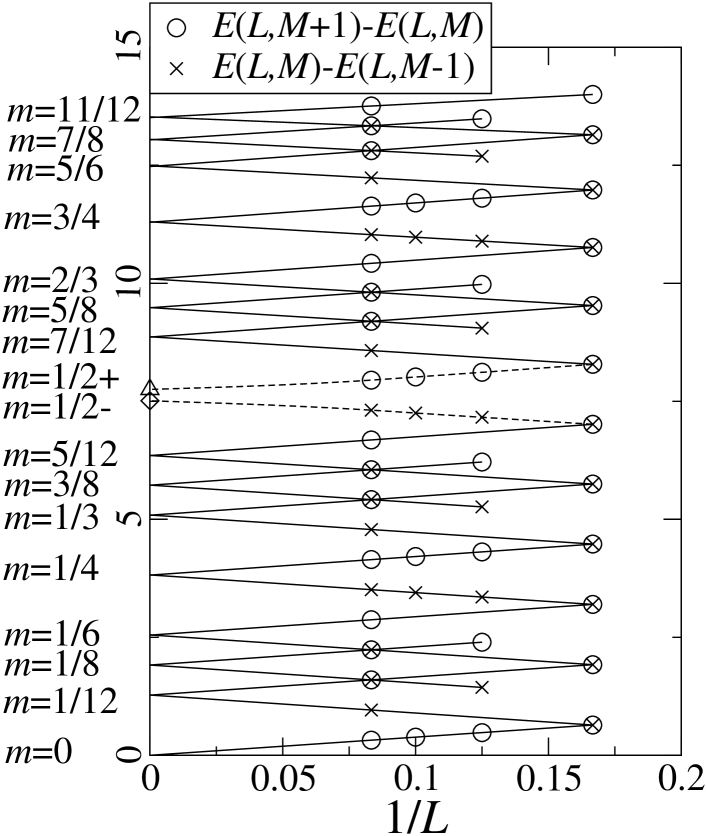
Figure 6: $E(L,M+1)-E(L,M)$ and $E(L,M)-E(L,M-1)$ plotted versus $1/L$ with fixed $m$ for $\lambda=1.0$ and $D=2.0$. Each two quantities seem to coincide to the magnetic field $H$ for $m$ in the thermodynamic limit. The extrapolated points for $m=1/2+$ and $m=1/2-$ correspond to the result of the Shanks transformation $H_{+}(1/2)$=7.75 and $H_{-}(1/2)$=7.51, respectively. Dashed curves are guides for the eye.

Using these methods, the magnetization curves in the thermodynamic limit are presented for $\lambda=1.0$ ($D$= 0.0, 1.0 and 2.0) in Fig. 7 and for $\lambda=2.0$ ($D$=0.0, 1.0 and 2.0) in Fig. 8.

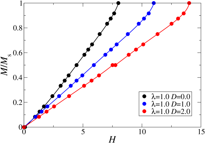
Figure 7: Magnetization curves for $\lambda=1.0$ obtained by the numerical diagonalization and the extrapolation methods; the equation (9) for gapless points and the Shanks transformation for plateau points. The large-$D$ plateau appears at $m=1/2$ for $D=2.0$, while no plateau for $D=$0.0 and 1.0. Curves are guides for the eye.

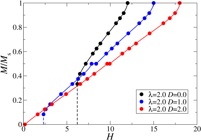
Figure 8: Magnetization curves for $\lambda=2.0$ obtained by the same method as Fig. 7. The Haldane and large-$D$ plateaus appear for $D$=1.0 and 2.0, respectively. The magnetization jump from $m=0$ due to the spin flop transition also occurs for $D=0.0$ and 1.0.

In Fig. 7 one of the precise estimations of the Haldane gap (0.0890)nakano2 is used as $H+(0)$ for $\lambda=1.0$ and $D=0$. As the ground state under $H=0$ for $\lambda=1.0$, $D=$1.0 and 2.0 is in the $XY$ phase,tonegawa1 the magnetic excitation should be gapless. In Fig. 8 the magnetization jump due to the spin flop transition occurs from $m=0$ for $D$=0.0 and 1.0, because the ground state under $H=0$ is in the Néel ordered phase.tonegawa1 As the precise magnetization curve around the jump is difficult to obtain by the numerical diagonalization, we assume that the magnetization jump occurs up to the smallest magnetization that is not skipped within the numerical diagonalization analysis. In any case the 1/2 magnetization plateau is quite small. Probably some precise magnetization measurement would be necessary to detect the 1/2 magnetization plateau of $S=2$ antiferromagnetic chain. If the Haldane plateau is too small to detect by the magnetization measurement, the ESR experiment to observe the edge spin effect at the doped impurity sitehagiwara1 would be useful.

VI BIQUADRATIC INTERACTION

It would be important to consider the biquadratic interaction $J_{\rm BQ}\sum_{j}(\mbox{\boldmath$S$}_{j}\cdot\mbox{\boldmath$S$}_{j+1})^{2}$, because it possibly stabilizes the magnetization plateau.penc The same level spectroscopy analysis as Figs. 2 and 4 is applied for the present model (2) including the biquadratic interaction. The result for $\lambda=1.0$ and $J_{\rm BQ}=0.05$ is shown in Fig. 9. It is found that the Haldane plateau phase appears even for $\lambda=1.0$, different from Fig. 2. The positive small biquadratic interaction is revealed to stabilize the Haldane plateau more than the large-$D$ one. Using the same method as Figs. 7 and 8, the magnetization curves are given for $\lambda=1.0$ in Figs. 10 (a) for $D=1.5$ (Haldane plateau phase) and (b) for $D=3.0$ (large-$D$ plateau phase), respectively. The magnetization curves for $J_{\rm BQ}=0.05$ and $J_{\rm BQ}=0.20$ are shown in Figs. 10 (a) and (b), respectively. It indicates that the biquadratic interaction enhances the Haldane plateau, while not the large-$D$ one. Thus some materials including the biquadratic interaction would be better candidates to exhibit the Haldane plateau. Actually the level spectroscopy analysis indicates that the Haldane plateau appears for $J_{\rm BQ}>J_{\rm BQc}=0.0723$ even in the isotropic case ($\lambda=1$ and $D=0$). We hope the Haldane plateau will be discovered as the field induced SPT phase. One of the candidate materials of $S=2$ antiferromagnetic chain is MnCl₃(bpy).hagiwara2 However, the single-ion anisotropy $D$ was reported to be much smaller than the plateau phase of the present result and the biquadratic interaction is not expected to exist unfortunately.

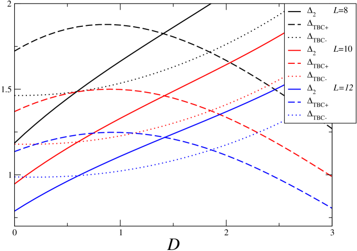
Figure 9: Level spectroscopy analysis for $\lambda=1.0$ and $J_{\rm BQ}=0.05$. Solid, dashed and dotted lines are for $\Delta_{2}$, $\Delta_{\rm TBC+}$ and $\Delta_{\rm TBC-}$, respectively. Black, red and blue lines are for $L=$ 8, 10 and 12, respectively. It is found that the Haldane plateau phase appears even for $\lambda=1.0$.

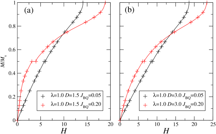
Figure 10: Magnetization curves for $\lambda=1.0$ obtained by the same method as Figs. 7 and 8: (a) for $D=1.5$ (Haldane plateau phase) and (b) for $D=3.0$ (large-$D$ plateau phase). Black and red curves are for $J_{\rm BQ}=0.05$ and $J_{\rm BQ}=0.20$, respectively. Curves are guides for the eye. When $J_{\rm BQ}$ increases, the Haldane plateau becomes much wider, while the large-$D$ plateau does not.

VII SUMMARY

In summary, the magnetization process of the $S=2$ antiferromagnetic Heisenberg chain with the exchange and single-ion anisotropies is investigated using the numerical exact diagonalization and the level spectroscopy analysis. As a result, the system possibly exhibits the 1/2 magnetization plateau due to Haldane mechanism, as well as the large-$D$ mechanism. The phase diagram of the $m=1/2$ state in the $\lambda$-$D$ plane is presented. The magnetization curves for several typical anisotropy parameters are also given. In addition the biquadratic interaction is revealed to enhance the Haldane plateau. We hope the present work would lead to the discovery of the field induced symmetry protected topological phase.

- (1) F. D. M. Haldane, Phys. Lett. 93A, 464 (1983).
- (2) F. D. M. Haldane, Phys. Rev. Lett. 50, 1153 (1983).
- (3) R. Botet and R. Jullien, Phys. Rev. B 27, 613 (1983).
- (4) M. P. Nightingale and H. W. J. Blöte, Phys. Rev. B 33, 659 (1986).
- (5) T. Sakai and M. Takahashi, Phys. Rev. B 42, 1090 (1990).
- (6) S. R. White and D. A. Huse, Phys. Rev. B 48, 3844 (1993).
- (7) S. Todo and K. Kato, Phys. Rev. Lett. 87, 047203 (2001).
- (8) H. Nakano and A. Terai, J. Phys. Soc. jpn. 78, 014003 (2009).
- (9) H. Nakano and T. Sakai, J. Phys. Soc. Jpn. 87, 105002 (2018).
- (10) X. Wang, S. Qin and L. Yu, Phys. Rev. B 60, 14529 (1999).
- (11) I. Affleck, T. Kennedy, E. H. Lieb and H. Tasaki, Phys. Rev. Lett. 59, 799 (1987).
- (12) I. Affleck, T. Kennedy, E. H. Lieb and H. Tasaki, Commun. Math. Phys. 115, 477 (1988).
- (13) T. Sakai and M. Takahashi, Phys. Rev. B 42, 4537 (1990).
- (14) W. Chen, K. Hida and B. C. Sanctuary, Phys. Rev. B 67, 104401 (2003).
- (15) Z.-C. Gu and X.-G. Wen, Phys Rev. B 80, 155131 (2009).
- (16) F. Pollmann, A. M. Turner, E. Berg and M. Oshikawa, Phys. Rev. B 81, 064439 (2010).
- (17) F. Pollmann, E. Berg, A. M. Turner and M. Oshikawa, Phys. Rev. B 85, 075125 (2012).
- (18) M. Oshikawa, J. Phys.: Condens. Matter 4, 7469 (1992).
- (19) H. Aschauer and U. Schollwöck, Phys. Rev. B 58, 359 (1998).
- (20) U. Schollwöck and Th. Jolicoeur, Europhys. Lett. 30, 493 (1995).
- (21) U. Schollwöck, O. Golinelli and Th. Jolicoeur, Phys. Rev. B 54, 4038 (1996).
- (22) T. Tonegawa, K. Okamoto, H. Nakano, T. Sakai, K. Nomura and M. Kaburagi, J. Phys. Soc. Jpn. 80, 043001 (2011).
- (23) K. Okamoto, T. Tonegawa, H. Nakano, T. Sakai, K. Nomura and M. Kaburagi, J. Phys.: Conf. Ser. 302, 012014 (2011).
- (24) K. Okamoto, T. Tonegawa, H. Nakano, T. Sakai, K. Nomura and M. Kaburagi, J. Phys.: Conf. Ser. 320, 012018 (2011).
- (25) K. Okamoto, T. Tonegawa, T. Sakai and M. Kaburagi, JPS Conf. Proc. 3, 014022 (2014).
- (26) K. Okamoto, T. Tonegawa and T. Sakai, J. Phys. Soc. Jpn. 85, 063704 (2016).
- (27) J. A. Kjäll, M. P. Zaletel, R. S. K. Mong, J. H. Bardarson, and F. Pollmann, Phys. Rev. B 87, 235106 (2013).
- (28) M. Oshikawa, M. Yamanaka and I. Affleck, Phys. Rev. Lett. 78, 1984 (1997).
- (29) T. Sakai and M. Takahashi, Phys. Rev. B 57, R3201 (1998).
- (30) A. Kitazawa and K. Okamoto, Phys. Rev. B 62, 940 (2000).
- (31) T. Sakai and M. Takahashi, Phys. Rev. B 43, 13383 (1991).
- (32) T. Sakai and M. Takahashi, J. Phys. Soc. Jpn. 60, 3615 (1991).
- (33) D. Shanks, J. Math. Phys. 34, 1 (1955).
- (34) M. N. Barber, in Phase trnasitions and critical phemonena, eds. C. Domb and J. M Lebowitz (Academic Press, New York, 1983) p.145.
- (35) M. Hagiwara, K. Katsumata, I. Affleck, B. I. Halperin and J. P. Renard, Phys. Rev. Lett. 65, 3181 (1990).
- (36) K. Penc, N. Shannon and H. Shiba, Phys. Rev. Lett. 93, 197203 (2004).
- (37) S. I. Shinozaki, A. Okutani, D. Yoshizawa, T. Kida, T. Takeuchi, S. Yamamoto, O. N. Risset, D. R. Talham, M. W. Meisel and M. Hagiwara, Phys. Rev. B 93 014407 (2016).