Dimers on Riemann surfaces I:
Temperleyan forests

Abstract

This is the first article in a series of two papers in which we study the Temperleyan dimer model on an arbitrary Riemann surface. The end goal of both papers is to prove the convergence of height fluctuations to a universal and conformally invariant scaling limit. In this part we show that the dimer model on the Temperleyan superposition of a graph embedded on the surface and its dual is well posed, provided that we add an appropriate number of punctures. We further show that the resulting dimer configuration is in bijection with an object which we call Temperleyan forest, whose law is characterised in terms of a certain topological condition. Finally we discuss the relation between height differences and Temperleyan forest, and give a criterion guaranteeing the convergence of the height fluctuations in terms of the Temperleyan forest.

1 Introduction

1.1 Background and main result

This paper is the first part of a series of two papers in which we show universality and conformal invariance of the Temperleyan dimer model on Riemann surfaces.

Given a finite graph $G$ (with an even number of vertices) and nonnegative weights $w=(w_{e})_{e\in E}$ on the edges, a dimer configuration is a perfect matching of the vertices along the edges of $G$. The dimer model is the random perfect matching obtained by sampling a dimer configuration $\bf m$ on $G$ with probability proportional to the product of the weights of the edges in the matching $\bf m$:

$$\mathbb{P}({\bf m})=\frac{\prod_{e\in{\bf m}}w_{e}}{Z},$$ (1.1)

where $Z$ is the partition function. If all the weights are equal to 1, $\mathbb{P}$ is simply a uniformly picked perfect matching. Following Thurston, a particularly convenient way to encode the dimer model on a planar bipartite graph is through a notion of height function. Informally, it is a real valued function defined on the faces of the graph, which is uniquely determined by the dimer configuration. This turns the dimer model into a model of discrete random surfaces. A central question in the study of the dimer model is to describe the fluctuations around the mean of the height function. It turns out that the height function of the dimer model is extremely sensitive to boundary conditions (see [26]). In the so-called liquid phase, the Kenyon–Okounkov conjecture predicts that the fluctuations of the height function around its mean are asymptotically given by a Gaussian free field in a certain nontrivial conformal gauge. Despite remarkable progress on this conjecture over the last decade, this remains an outstanding problem in all but a handful of cases: see [4, 18, 25, 30, 32] for examples of models where this is already shown, and see [7, 34] for an introduction to the Gaussian free field. We emphasise that, given the extreme sensitivity of the model to its boundary conditions, the occurrence of a universal limit such as the Gaussian free field is to some extent very surprising.

The goal of this paper is to describe the fluctuations of the height function for certain graphs embedded on Riemann surfaces of finite topological type, i.e., with finitely many handles and holes. Our assumptions on these graphs ensure that the dimer model is liquid on the entire Riemann surface and the conformal gauge is simply the identity; we call the resulting dimer model Temperleyan, and we say that the sequence of graphs $G^{\#\delta}$ is a Temperleyan discretisation of the surface. Even though this assumption simplifies the problem, conformal invariance in the scaling limit is by no means obvious; for instance, in the simply connected setting and for the square lattice, this is in fact precisely the content of Kenyon’s landmark paper [24].

Before we give a simplified statement of the main theorem, we point out that in the context of a Riemannian surface $(M,g)$, the height function becomes a height one-form $h^{\#\delta}$: that is, the gradient $\nabla h^{\#\delta}$ is well-defined but this gradient does not derive itself from a single-valued function on the surface. Instead it can be viewed as the gradient of a (single-valued) function defined on the universal cover of the surface. For concreteness we will denote by $h^{\#\delta}$ the associated function on the universal cover of the surface. Readers who prefer it can however equivalently think of $h^{\#\delta}$ as the random one-form on $M$ associated to the dimer configuration. (See Sections 2.4 and 6.1 for precise definitions.) The function $h^{\#\delta}$ is the central object of this sequence of papers, and we still refer to it as the height function.

Our main theorem, stated informally below, confirms that the dimer model admits a universal scaling limit on Riemann surfaces. This scaling limit is furthermore conformally invariant.

Theorem 1.1.

Let $(M,g)$ denote a bounded Riemann surface, possibly with a boundary, which is not the sphere or a simply-connected domain. Let $G^{\#\delta}$ be a sequence of Temperleyan discretisations of $M$ satisfying the invariance principle and a crossing estimate for random walk described in Section 2.3. Let $h^{\#\delta}$ denote the height function of the dimer model on $G^{\#\delta}$. For all smooth compactly supported test functions $f$,

$$\int(h^{\#\delta}-\mathbb{E}(h^{\#\delta}))f$$

converges as $\delta\to 0$ in law and the limit is conformally invariant and independent of the sequence $G^{\#\delta}$.

The precise assumptions on the surface $M$ will be given in Section 2.1, the meaning of Temperleyan discretisations and our precise assumptions on the sequence $G^{\#\delta}$ can be found in Section 2.3. Finally, recall that the smooth test function $f$ is taken on the universal cover $M^{\prime}$ of $M$, so that the integration takes place on $M^{\prime}$ (equipped e.g. with Lebesgue measure). See Sections 2.4 and 6.1 for details. We refer to Theorem 6.1 for the complete version of the theorem.

Brief outline.

Our general approach to study height fluctuations on Riemann surfaces is motivated and inspired by our earlier work [4] connecting the dimer model to imaginary geometry in the simply connected setting. Let us recall the main idea of that work briefly in the original simply connected setting, before explaining how this relates with and differs from the case of Riemann surfaces.

1. The starting point of [4] is Temperley’s bijection, which relates the dimer model on a Temperleyan discretisation of a simply connected domain to a pair of dual uniform spanning trees with respectively wired and free boundary conditions. Furthermore, the height function of the dimer model can be determined relatively simply from the associated pair of spanning trees: roughly speaking, the height difference between two points is simply the total winding (sum of turning angles) of the unique path connecting these points in either tree.

2. The second observation is that, as follows from the landmark paper of Lawler, Schramm and Werner [29], paths between points in the wired uniform spanning tree (UST) have a scaling limit which may be described in terms of Schramm–Loewner Evolutions with parameter $\kappa=2$ or SLE₂ for short.

3. Finally, in the continuum, there is a coupling known as imaginary geometry between SLE_κ curves and an appropriate multiple of the Gaussian free field. In this coupling, the values of the GFF may informally be identified as the winding of the associated SLE curves (note that this requires careful interpretation, since the Gaussian free field is not defined pointwise and SLE_κ paths are not smooth). Nevertheless, this coupling can be thought of as a continuous form of Temperley’s bijection in the case $\kappa=2$.

The strategy of [4] is to exploit Temperley’s bijection on the one hand, and Imaginary Geometry on the other hand, to show that the winding of paths in a UST is indeed given by the appropriate multiple of the Gaussian free field asymptotically (essentially, one has to show that we can exchange the order of taking limits, or that a diagram commutes). This strategy is very robust; in particular it does not appeal to the more solvable aspects of the dimer model. Indeed, the convergence of loop-erased random walks (which describe the branches of a wired UST at the discrete level) to SLE₂ is known in great generality.

Roughly speaking, we wish to implement a similar approach in the case of Riemann surfaces. However, it should be clear that each part will be substantially different in this new setup.

• To begin with, we observe that Temperley’s bijection is local and so may be applied on a Riemann surface to output a pair of random subgraphs that are dual to one another and locally tree-like, and which we call Temperleyan self-dual pair. While in the simply connected case these are of course just dual spanning trees, the nature (i.e. state space) of the Temperleyan self-dual pair on a Riemann surface is a priori not entirely clear, and its law even less so. Our first result will be a characterisation of the Temperleyan self-dual pair. We also describe its law explicitly, which has a simple and concise expression. It turns out that one of the two components, which we call the Temperleyan cycle-rooted spanning forest or Temperleyan CRSF for short, determines the other (and hence the entire dimer configuration) uniquely, and also has a tractable law. Essentially, a Temperleyan CRSF is a random spanning subgraph in which every cycle is noncontractible, and satisfying a certain further topological condition. The introduction and study of Temperleyan CRSFs occupies us throughout both articles in this series.

• A second problem is that the connection between height function and winding is not as straightforward as in the simply connected case; in particular, in addition to the already mentioned fact that only the gradient of the height function is well defined (leading to a multivalued height function), there may not be a path connecting two given points in the Temperleyan CRSF, even when they are neighbours. We thus need to develop a systematic method for computing the height function given the Temperleyan CRSF.

• The next difficulty is to obtain a scaling limit result for our Temperleyan CRSF. Let us immediately note here that there are specific difficulties with defining variants of SLE on surfaces since the simply-connected uniformisation theorem lies at the heart of the standard definition of SLE. In addition, if we were to follow the blueprint of [4] one would also need to establish a version of Imaginary geometry for Riemann surfaces, an endeavour which seems out of reach with current techniques. Fortunately, we are in fact able to entirely bypass this step because it turns out that the (discrete) estimates needed anyway to exchange limits are strong enough to imply convergence regardless of any information in the continuum. Clearly, the downside of this approach that we cannot hope to describe the law of the limit in this manner.

The topological and geometric structures of the surface $M$ raise substantial specific difficulties at each of the steps of this roadmap. In this first paper we develop the relevant discrete/combinatorial arguments corresponding to the first two bullet points above. The second companion paper in this sequence, [5], is devoted to the proof of convergence of the Temperleyan CRSF in the scaling limit. This is the most involved step at the technical level, but can be read essentially independently.

1.2 Relation with previous work

One of the first rigourous works on the dimer model on Riemann surfaces is the inspiring paper by Boutillier and de Tilière [9], who were motivated by nonrigourous physics predictions based on the Coulomb gas formalism (see e.g. [16] and the references in [9]). They described the topological part of the fluctuations in the dimer model on the honeycomb lattice on the torus. This was complemented some years later by the fundamental paper of Dubédat [18], in which the full law of the limiting height fluctuations was described for isoradial graphs on the flat torus, and identified as a so-called compactified Gaussian free field. Dubédat also conjectured a greater form of universality beyond the isoradial setting; such a universality statement was subsequently proved by Dubédat and Gheissari [19] but only for the topological part of fluctuations on the torus. Note that in particular our Theorem 1.1 settles this conjecture of Dubédat.

We point out that all techniques in the paper mentioned above, based on Kasteleyn theory (in contrast with our approach), are very specific to the case of the torus and cannot easily be adapted to general Riemann surfaces. The paper of Cimasoni [10] shows that for general surfaces of genus $g$ (and no boundary), the partition function of the dimer model becomes a weighted (in fact, signed) sum of $2^{2g}$ determinants of Kasteleyn matrices in which the orientation has been reversed along some of the $2g$ cycles forming a basis of the first homology group of the surface. The signs in front of the determinants themselves form a nontrivial algebraic topological invariant of the surface which Cimasoni, remarkably, was able to identify in terms of the so-called Arf invariant. (In the case of the torus and the honeycomb lattice, this goes back to the work of Boutillier and de Tilière [9].) This illustrates the difficulty in generalising the Kasteleyn approach to general surfaces. See also [1, 11, 12, 14] for related results.

The above difficulty illustrates the well known fact that the dimer models becomes “less integrable” as the genus of the surface increases, or at any rate integrability becomes harder to exploit. Our approach is not dependent on integrability or solvability and this accounts in large part for the fact that we are able to tackle generic Riemann surfaces (in contrast with methods based on Kasteleyn theory or interacting particle systems). This is not to say that the difficulties caused by the increased complexity of the surface vanish entirely, but they manifest themselves in a different manner, which boil down to the following issue. As we will describe in more details in Section 2, a Temperleyan discretisation of the surface is the graph resulting from the superposition of a graph $\Gamma$ embedded on the surface and its dual. The resulting graph is (locally) bipartite, with its black vertices being given by the vertices and faces of $\Gamma$, and the white vertices being given by the edges of $\Gamma$. However, a straightforward calculation using Euler’s formula shows that this does not admit a dimer covering unless we remove $2g+b-2=|\chi|$ white vertices from the graph (where $g$ is the genus and $b$ the number of boundary components, and $\chi$ is the Euler characteristic); these can be thought of as punctures in the surface, or monomers. Note that the number of punctures increases with the complexity of the surface, but when the surface is a torus or an annulus no such puncture needs to be removed. Roughly speaking, each puncture or monomer is responsible for an extra topological condition which the Temperleyan forest is required to satisfy; in particular in the case of a torus or an annulus, the Temperleyan forest is not conditioned on any degenerate event and boils down to the simpler notion of cycle-rooted spanning forest studied by Kassel and Kenyon in [23].

The necessity to remove a certain number of punctures from the surface in order to formulate the Temperleyan dimer model has a geometric flavour which is reminiscent of Liouville conformal field theory, in which correlation functions are only well defined with the appropriate number of singularities (known in that context as insertions). The required number of insertions is specified by the so-called Seiberg bounds, see e.g. [15] on the sphere and [20] for Riemann surfaces (see also [7] for an introduction). As is the case here, the number of punctures is entirely specified by the topology of the surface, but in a way that is in some sense opposite to ours: indeed the required number of insertions is an increasing function of $\chi$ in Liouville CFT, whereas it is decreasing here.

This difference can be understood informally as follows. To first order, Liouville CFT may be viewed as yielding a random metric which is approximately hyperbolic (this can for instance be made rigourous in the semiclassical limit where the parameter $\gamma\to 0$, see [28]). However, without adding conical singularities at a certain number of points, it may not be possible to equip the surface with a metric of constant negative Ricci curvature, as follows from the Gauss–Bonnet theorem. By contrast, the Temperleyan dimer model is trying to equip the surface with a flat metric, a fact which will be particularly apparent when we relate the height function to the winding of the Temperleyan forest in Section 4 (note that the winding is computed on the universal cover, where curvature effects are ignored). But on a hyperbolic surface (i.e., when $\chi<0$), no flat metric exists, again by the Gauss–Bonnet theorem. In summary, Liouville CFT may be viewed as trying to build a hyperbolic metric on a surface which may be parabolic or elliptic, whereas the Temperleyan dimer model tries to impose a flat metric on a surface which may be hyperbolic. In both cases the difficulty is resolved by puncturing the surface at an appropriate number of singularities. (The above parallel between Liouville CFT and dimer model is also to be compared with the two couplings between SLE and Gaussian free fields given respectively by the so-called forward and reverse couplings; the forward coupling describes Liouville conformal field theory whereas the reverse coupling describes imaginary geometry).

1.3 Overview of the proof and organisation of the paper

• In Section 2, we recall some basic facts about dimers on surfaces. Sections 2.1 and 2.2 contain small reminders about Riemann surfaces in two dimensions. We introduce precisely our discrete setup in Section 2.3. As one of the main difference with the classical case is that the height function now becomes multivalued we recall in Section 2.4 the language of height one-forms on graphs which is a classical way to handle such multivalued functions. In Section 2.5, we introduce another way to deal with multivalued functions by lifting them to single-valued functions on the universal cover. This is in practice easier to deal with, and we mainly work with this lift in this article. We also illustrate how an application of the Hodge decomposition theorem allows us to decompose the (multivalued) height function on the surface into a single-valued function (scalar component) and a canonical representative of the “multivalued (or topological) part”, the so-called instanton component. In Section 2.6, we recall the notions of windings of curves which were developed in our previous article [4].

• In Section 3, we introduce the generalisation of Temperley’s bijection to Riemann surfaces. Section 3.1 contains the bijection itself which, as mentioned above, uses a new type of object which we call a Temperleyan CRSF or Temperleyan forest for short. We also provide in Section 3.2 a simple criterion for a CRSF to be Temerleyan which is the basis of [5].

• In Section 4, we carefully develop the relation between the height differences and the winding of Temperleyan forests; in spite of the curvature of the surface such a connection remains true if one considers a natural embedding of the graph on the universal cover of the surface. This is in the spirit of the work of Kenyon–Propp–Wilson [27], who treated the (planar) simply connected case. In that case of course the bijection is with a uniform spanning tree. Compared to that work there are two additional points that we need to handle. The first one is that the edges of the graph cannot be assumed to be straight lines as in [27]. The second and more significant one is that there are additional terms coming from the fact that the forest is not connected: given points $x$ and $y$ on the universal cover, the height difference $h(x)-h(y)$ (which is unambiguously defined) is essentially given by the intrinsic winding of any path connecting $x$ to $y$, plus additional discontinuities every time the path jumps between components. The resulting key formula is stated in Theorem 4.10 (see also Lemma 4.6).

• In Section 5, we extend our local and global coupling results from [4] to the framework of Riemann surfaces. This coupling is a key ingredient of our approach, which allows us to show that given a finite number of points $(z_{i})_{1\leq i\leq k}$ on the surface (or, rather, their lifts to the universal cover), the respective geometries of the CRSF in a neighbourhood of these $k$ points decouple and are independent. Clearly, such an independence can only be expected to hold at distances smaller than the distances between the $z_{i}$’s, but if the points are macroscopically far apart this still leaves a lot of room. The strength of this coupling is that it holds at an essentially optimal scale. More precisely, the independence property holds in neighbourhoods whose size is random and comparable to the distance between the $z_{i}$’s, with an exponential control on the number of additional finer scales required for the independence to hold.

  The argument in [4] was based on relatively soft estimates about LERW, and it is not difficult to adapt them to this setting. There is one additional technicality however, which can be summarised as follows. A basic estimate needed for the argument is a polynomial control on the probability that a LERW starting from $u$ comes close to a given point $v$ (Proposition 4.11 in [4]). In [4] we could exploit the fact that if the random walk starting from $u$ comes within $e^{-n}$ of $v$ then it has a positive probability to make a loop around $v$ at all scales $e^{-n+1},\ldots,1$ subsequently, which erases the portion of the walk coming close to $v$ in the loop-erasure. This results in an exponentially small probability that the loop-erasure comes with distance $e^{-n}$ of $v$. However, in the setup of Riemann surfaces, the walks also stop when it makes a non-contractible loop. Therefore if a random walk comes within distance $e^{-n}$ of $v$, there is a possibility that the walk completes a noncontractible loop shortly after, say at distance $e^{-n+m}$ from $v$, with $m\ll n$. In this case there are in principle no remaining constraints on larger scales, and we do not get a sufficiently good bound on the probability that the path comes close to $v$. The argument needed to overcome this technical difficulty is given in Lemma 5.3.

• In Section 6, we finish by proving our main convergence result Theorem 6.1. Sections 6.2 and 6.3 contain some a priori technical estimates on winding of the CRSF branches on the universal cover. Finally in Section 6.4, we finish the proof of Theorem 6.1. This proof shares similarities with the argument in [4], but with the difference that we cannot rely on imaginary geometry to identify the limit.

• Finally, appendix A contains some geometric facts about spines in the CRSF (that is, the lift to the universal cover of a cycle of the CRSF). It is shown that such spines, in the hyperbolic case, form simple chords in the unit disc (simple paths joining two boundary points) or a loop touching the boundary at a single point. This basic fact (stated as Lemma 4.9 but proved in the appendix) underlies much of the discussion connecting winding to height differences. The proof relies on some arguments from the classical theory of Riemann surfaces.

Acknowledgements

The authors are grateful to Antoine Dahlqvist and Julien Dubédat for a number of useful discussions. NB’s is supported by FWF grant P33083, “Scaling limits in random conformal geometry”. GR’s research is supported by NSERC 50311-57400. BL’s research is supported by ANR-18-CE40-0033 “Dimers”. The paper was finished while NB was in residence at the Mathematical Sciences Research Institute in Berkeley, California, during the Spring 2022 semester on Analysis and Geometry of Random Spaces, which was supported by the National Science Foundation under Grant No. DMS-1928930.

2 Background and setup

2.1 Riemann surfaces and embedding

In this article, we work with a 2-dimensional orientable connected Riemann surface $M$ equipped with a Riemannian metric $d_{M}$ satisfying the following properties.

• $M$ is of finite topological type, meaning that the fundamental group $\pi_{1}(M)$ is finitely generated. In other words, we assume that the surface has finitely many “handles” and “holes”.

• $M$ can be compactified by specifying a boundary $\partial M$. We denote by $\overline{M}$ the compactified Riemann surface with the boundary. More precisely, every point is either in the interior and hence has a local chart homeomorphic to $\mathbb{C}$ or is on the boundary and has a local chart homeomorphic to the closed upper half plane $\bar{\mathbb{H}}$. Also there are finitely many such charts which cover the boundary. Note that this condition implies that $M$ has no punctures. (However for future reference, we note here that we will later introduce punctures on $M$ which will align with the removed vertices of Temperleyan graphs. The resulting punctured manifold will be denoted by $M^{\prime}$.)

• The metric in $M$ extends continuously to $\partial M$. In other words, recall that the metric inside $M$ can be represented locally in isothermal coordinates as $e^{\rho}|dz|^{2}$ for a smooth function $\rho$ and we assume that $\rho$ extends continuously to $\partial M$.

We say $M$ is nice if $M$ satisfies the above properties. Note that continuous extension of the metric to the boundary means we exclude surfaces such as the hyperbolic plane, and will technically simplify certain topological issues later when we deal with the Schramm topology.

Classification of surfaces

Riemann surfaces can be classified into the following classes depending on their conformal type (see e.g. [17] for an account of the classical theory):

• Elliptic: this class consists only of the Riemann sphere, i.e., $M\equiv\hat{\mathbb{C}}$

• Parabolic: this class includes the torus, i.e., $M\equiv\mathbb{T}=\mathbb{C}/(\mathbb{Z}+\tau\mathbb{Z})$ where $\Im(\tau>0)$), the cylinder $M\equiv\mathbb{C}\setminus\{0\}$, and the complex plane itself (or the Riemann sphere minus a point), $M\equiv\mathbb{C}$.

• Hyperbolic: this class contains everything else. This includes examples such as the two-torus, the annulus, as well as proper simply connected domains in the complex plane, etc.

The proofs in this paper (and its companion [5]) are concerned with the hyperbolic case (subject to the above conditions) as well as the case of the torus so from now on we always assume that $M$ is such a manifold. We note that the case of simply connected domain in $\mathbb{C}$ is covered in our previous work [4].

2.2 Universal cover

The universal cover $\tilde{M}$ of the Riemann surface $M$ will play an important role in our analysis. In the cases that we will analyse, due to the above classification, the universal cover can be classified as follows:

• $\tilde{M}\equiv\mathbb{C}$ in the parabolic case of the torus;

• $\tilde{M}\equiv\mathbb{D}$ (the unit disc) in all remaining non-simply connected hyperbolic cases.

From now on we assume, unless otherwise explicitly stated, that we are only dealing with these cases. We also recall here the classical Riemann uniformisation theorem: $M$ is conformally equivalent to $\tilde{M}/F$ where $F$ is a discrete subgroup of the Möbius group. In case of the torus, this discrete subgroup is isomorphic to $\mathbb{Z}^{2}$ and the generators specify translations in the two directions of the torus. In the hyperbolic case, this class of subgroups is much bigger and are known as Fuchsian groups (see e.g. [17] and appendix A). This particular representation of a surface, sometimes called a Fuschian model, will be particularly convenient to describe the scaling limits of Temperleryan or cycle-rooted spanning forests in the universal cover, rather than on the surface itself. This is essential for our purposes since the lack of curvature in the cover allows us to compute winding in a straightforward manner.

Let $p:\tilde{M}\to M$ be the covering map associated with the Riemann uniformisation theorem. That is, in the hyperbolic case, we write $M=\mathbb{D}/F$ and $p:\mathbb{D}\to M$ is the canonical projection which is then conformal. In the case of the torus, $p:\mathbb{C}\to M$ is the standard projection from the plane onto the torus and is also conformal. We recall here that the covering map acts discretely, in the sense that for every $z\in M$, there exists a neighbourhood $N$ containing $z$ so that $p$ is injective in every component of $p^{-1}(N)$.

We will require the graphs we are working with to be embedded on $M$ in a way that preserve its topology and geometry. Essentially the topological conditions will be that edges cannot cross, all interior faces must be homeomorphic to discs and the boundary of the manifold must correspond to simple loops on the graph, as outlined in the next section.

2.3 Discretization setup

Let $\Gamma$ be a graph which is properly embedded on a Riemann surface $M$ with $b$ holes and $g$ handles (see Section 2.1 for precise assumptions on the $M$). Let $\Gamma^{\dagger}$ be its planar dual. A face of $\Gamma$ (resp. $\Gamma^{\dagger}$) is a connected component in $M$ of the complement of the embedded graph $\Gamma$ (resp. $\Gamma^{\dagger}$). We assume that $\Gamma^{\dagger}$ is embedded on $M$ so that every vertex of $\Gamma^{\dagger}$ is in a face of $\Gamma$ and every edge $e$ of $\Gamma$ is crossed by a single edge $e^{\dagger}$ of $\Gamma^{\dagger}$ which joins the two faces incident to $e$. (Later, when we consider a random walk on $\Gamma$ we will allow the jump probabilities to be non-uniform and non-reversible, but for now $\Gamma$ and $\Gamma^{\dagger}$ are both unweighted, undirected graphs).

We assume that $\Gamma$ and $\Gamma^{\dagger}$ are faithful to the topology of the surface in the following sense. We require all faces of $\Gamma$ and $\Gamma^{\dagger}$ whose boundary does not intersect $\partial M$ to be homeomorphic to a disc. We also require all faces of $\Gamma^{\dagger}$ whose boundary intersects $\partial M$ (we call those faces outer faces) to be homeomorphic to an annulus. In other words, we have a boundary vertex of $\Gamma$ corresponding to each hole (let $\partial\Gamma$ denote the set of such vertices), and each hole is surrounded by a cycle in $\Gamma^{\dagger}$ which we call boundary cycle and which we denote by $\partial\Gamma^{\dagger}$.

Figure 1: The graphs $\Gamma,\Gamma^{\dagger}$, and $G$. In the leftmost picture $\Gamma$ is pictured in red and $\Gamma^{\dagger}$ in black. In the rightmost picture note that vertices in $B$ appear as either a black or a red dot. The graph is Temperleyan in the sense that all the $B$ vertices on the boundary are of one type only, namely black (i.e., vertices of $\Gamma$).

We assign an oriented weight $w(e)=w_{\Gamma}(e)$ to every oriented edge of $\Gamma$. This defines a continuous time Markov chain on $\Gamma$ where for every edge $(x,y)$ in $\Gamma$, the chain jumps from $x$ to $y$ at rate $w(x,y)$, and with a slight abuse of terminology we will from now on refer to this chain as the random walk on $\Gamma$. Note that we defined it in continuous time for simplicity but we will in fact always be interested only by the geometry of its paths so its time parametrisation is mostly irrelevant. With a slight abuse of notations, we will often identify the trajectory of the random walk (or other processes such as loop-erased paths) with the continuous path obtained from the set of edges used by the walk, either seen as a path or as a subset of $M$. Similarly, with a slight abuse of notation, we will use direct image notations to denote sub-paths of the random walk, i.e if $s<t$ are two times, we will denote by $X[s,t]$ the path followed by the random walk between times $s$ and $t$. Finally we will always stop the random walk whenever it reaches a boundary vertex so we assume that all oriented edges starting at such a vertex have weight $0$. We emphasize that there are no weights on the dual graph $\Gamma^{\dagger}$ and indeed we will never consider the random walk on the dual graph.

Remark 2.1.

To explain the asymmetry between $\Gamma$ and $\Gamma^{\dagger}$, we point out that $\Gamma$ can be thought of as a graph that is wired at the boundary of $\partial M$ whereas $\Gamma^{\dagger}$ has free boundary conditions.

In order to apply locally the bijection between dimers and (a variant of) spanning trees, we need to define the superposition of $\Gamma$ and $\Gamma^{\dagger}$. We introduce a new set of vertices $W$ at each point where some edge $e$ and dual edge $e^{\dagger}$ intersect. Define the graph $\hat{G}$ whose vertices are $V=V(\Gamma)\cup V(\Gamma^{\dagger})\cup W$ and the edges given by joining every vertex in $W$ which is on the edge $e$ with the endpoints of $e$ and $e^{\dagger}$ (in other words, each pair of edges $e$ and $e^{\dagger}$ corresponds to four edges in $\hat{G}$). We call $\hat{G}$ the superposition graph. Then define $G$ to be the graph where we remove from $\hat{G}$ the boundary vertices $\partial\Gamma$ and its corresponding half edges. See Figure 1 for an illustration. Clearly, $G$ is a bipartite graph where we take $W$ to be the set of white vertices and the rest to be black. Also every non-outer face of $G$ is bounded by $4$ edges (i.e. every non-outer face is a quadrangle). We can naturally define unoriented weights on $G$ from the ones on $\Gamma$. If $w$ is the white vertex in the middle of the edge $(x,y)$ of $\Gamma$, we set $w_{G}(x,w)=w_{\Gamma}(x,y)$ and $w_{G}(y,w)=w_{\Gamma}(y,x)$ while $w_{G}(e)=1$ if $e$ is part of an edge of $\Gamma^{\dagger}$.

We will prove in Section 3 that if the manifold $M$ is not a torus or an annulus, one must introduce punctures in the graph $G$ for it to even admit dimer coverings. More precisely we will remove finitely many white vertices from $G$ and call a removed vertex and the edges associated with it a puncture (equivalently, the puncture may be thought of as forcing the vertex to be a monomer instead of in a dimer edge). Note that each puncture creates an octagon $G$ consisting of four white vertices, two black vertices from $\Gamma$ and two black vertices from $\Gamma^{\dagger}$ (see Figure 2). We will call the resulting graphs respectively $G^{\prime},\Gamma^{\prime},(\Gamma^{\dagger})^{\prime}$ and we call the manifold obtained by removing the white vertices $M^{\prime}$. We will see later in Section 3 that the number of punctures we remove must be ${\sf k}=|\chi|$ where $\chi$ is the Euler characteristic of $M$. When this is the case we will call $G^{\prime}$ a Temperleyan graph on $M$ or Temperleyan discretisation of $M$.

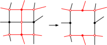
Figure 2: Removing a white vertex (puncture) to create the dimer graph $G^{\prime}$.

When considering scaling limits, we will of course consider a sequence of graphs $\Gamma^{\#\delta},(\Gamma^{\dagger})^{\#\delta}$, $G^{\#\delta}$ from the setup above. We now introduce our assumptions on such a sequence.

Let $p:\tilde{M}\mapsto M$ be a conformal lift to the universal cover $\tilde{M}$, which is either the unit disc or the whole plane. In the end the choice of this lift does not affect the following assumptions, see Remark 2.3 for a precise discussion about this lift and also about the lift of the punctured manifold.

1. (Bounded density) There exists a constant $C$ independent of $\delta$ such that for any $x\in M$, the number of vertices of $\Gamma^{\#\delta}$ in the ball $\{z\in M:d_{M}(x,z)<\delta\}$ is smaller than $C$.

2. (Good embedding) The edges of the graph are embedded as smooth curves and for every compact set $K\subset\tilde{M}$, the intrinsic winding of every edge in the lift $\tilde{\Gamma}^{\#\delta}$ intersecting $K$ is bounded by a constant $C=C_{K}$ depending only on $K$. (Note that this allows edges to wind quite a bit near holes.)

3. (Invariance principle) As $\delta\to 0$, the continuous time random walk $\{\tilde{X}_{t}\}_{t\geq 0}$ on $\tilde{\Gamma}^{\#\delta}$ started from a nearest vertex to $0$ satisfies:

   $${(\tilde{X}_{t/\delta^{2}})_{t\geq 0}}\xrightarrow[\delta\to 0]{(d)}(B_{\phi(t)})_{t\geq 0}$$

   where $(B_{t},t\geq 0)$ is a two dimensional standard Brownian motion in $\tilde{M}$ (killed when it leaves $\tilde{M}$, if $\tilde{M}=\mathbb{D}$) started from $0$, and $\phi$ is a nondecreasing, continuous, possibly random function satisfying $\phi(0)=0$ and $\phi(\infty)=\infty$. The above convergence holds in law in Skorokhod topology.

   We remark that the above condition is equivalent to asserting that simple random walk from some fixed vertex converges to Brownian motion on the Riemann surface itself up to time parametrisation (see e.g. [22]).

   

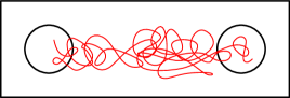
   Figure 3: An illustration of the crossing condition.

4. (Uniform crossing estimate). Let $R$ be the horizontal rectangle $[0,.3]\times[0,.1]$ and $R^{\prime}$ be the vertical rectangle $[0,.1]\times[0,.3]$. Let $B_{1}:=B((.05,.05),0.025)$ be the starting ball and $B_{2}:=B((.25,.05),.025)$ be the target ball (see Figure 3).

   The uniform crossing condition is the following. There exist universal constants $\delta_{0},\alpha_{0}>0$ such that for every compact set $K\subset M$, there exists a $\delta_{K}$ such that for all $\delta\in(0,\delta_{K})$ the following is true. Let $\tilde{K}$ be the lift of $K$. Let $R^{\prime\prime}$ be a subset of one of the connected components of $\tilde{K}$ and is a translation of $cR$ or $cR^{\prime}$ where $c\geq\delta/\delta_{0}$. Let $B_{1}^{\prime\prime}$ (resp. $B_{2}^{\prime\prime}$) be the same translation of $cB_{1},cB^{\prime}_{1}$ (resp. $cB_{2},cB_{2}^{\prime})$. For all $v\in\tilde{\Gamma}^{\#\delta}\cap B_{1}^{\prime\prime}$,

   $$\mathbb{P}_{v}(\tilde{X}\text{ hits }B^{\prime\prime}_{2}\text{ before exiting }R^{\prime\prime})>\alpha_{0}.$$ (2.1)

   In what follows, sometimes for a compact set $K\subset\tilde{M}$, we will write $\delta_{K}$ to mean $\delta_{p(K)}$ as defined above.

5. (punctures) We remove $\sf k=|\chi|$ many points from $M$ and call the resulting surface $M^{\prime}$, where $\chi$ is the Euler characteristic of $M$. We assume that each of the ($\sf k$ many) monomers (white vertices removed from $\hat{G}$ to obtain $G^{\prime}$) converge to a unique puncture as $\delta\to 0$.

Remark 2.2.

We also remark here that the invariance principle assumption item iii actually implies something stronger in combination with the other assumptions: for any point $x$ in $\tilde{M}$, the random walk started from a vertex $x^{\#\delta}$ nearest to $x$ converges to a Brownian motion started from $x$ up to a time change as above. This is a consequence of the fact that random walk from 0 comes close to $x$ with uniformly positive probability using the crossing estimate and the strong Markov property of Brownian motion.

In case $\partial M\neq\emptyset$, recall that the set of boundary cycles $(\partial\Gamma^{\dagger})^{\#\delta}$ corresponds to the connected components of $\partial M$. One consequence of the Invariance principle assumption (item iii) is that each boundary cycle converges in the Hausdorff metric (induced by $d_{\bar{M}}$) to the associated component of $\partial M$.

Sometimes we drop the superscript $\delta$ from $\Gamma^{\#\delta},(\Gamma^{\dagger})^{\#\delta}$ for clarity, when there is no possibility of a confusion.

Remark 2.3.

By the uniformisation theorem of Riemann surfaces, we know that there exists a conformal map from the Riemann surface $\tilde{M}/F$ to $M$ where $F$ is a Fuchsian group which is a discrete subgroup of the group of Möbius transforms on $\tilde{M}$. In the case of the torus, this subgroup is simply a group of translations isomorphic to $\mathbb{Z}^{2}$. In the hyperbolic case $F$ is a subgroup of the group of Möbius transforms of the unit disc $\mathbb{D}$. Such a conformal map is unique up to conformal automorphisms (i.e. Möbius transforms) of the unit disc. In other words, if $F,F^{\prime}$ are two Fuchsian groups such that $M$ is conformally equivalent to both $\mathbb{D}/F$ and $\mathbb{D}/F^{\prime}$ then there exists a Möbius map $\phi:\mathbb{D}\mapsto\mathbb{D}$ such that $F^{\prime}=\phi^{-1}\circ F\circ\phi$. Since we have fixed a lift $p$, we have defined $F$ uniquely.

We also remark that in item iii, we only require convergence up to time change, and hence this assumption depends only on the conformal type of the metric. Finally, one could be worried about the fact that in item iv, the probability $\alpha_{0}$ is uniform over the position and scale of the rectangle despite the distortion between two copies of the same set $K\subset M$. However note that the image of a rectangle by a Möbius transform is made of $4$ circular arcs and is crossed by Brownian motion with the same probability as the original rectangle, so our assumption is natural in this sense.

Finally, note also that while we have stated these assumptions on the universal cover of $M$, we could equivalently stated these assumptions on the universal cover of the punctured surface $M^{\prime}$ instead. The fact that these assumptions are equivalent can be checked using the fact that there is a map from the universal cover of $M^{\prime}$ to $\tilde{M}\setminus p^{-1}(\{x_{1},\ldots,x_{\sf k}\})$ (where $x_{1},\ldots,x_{\sf k}$ is the set of punctures) which is locally a conformal bijection.

In summary, we could work with any lift (i.e. any choice of $F$) both for the punctured and the non-punctured manifold and we fix a particular choice of this lift and call it $p$ if lifting to $M$ or $p^{\prime}$ if lifting to $M^{\prime}$ for concreteness; in fact, with a small abuse of notation we will use $p$ throughout.

2.4 Height function and forms

A flow $\omega$ is an antisymmetric function on the oriented edges $\vec{E}$ of $G$, i.e., for every oriented edge $(u,v)$, $\omega(u,v)=-\omega(v,u)$. The total flow out of a vertex $v$ is defined to be $\sum_{w\sim v}\omega(v,w)$. Similarly, the total flow into a vertex $v$ is defined to be $\sum_{w\sim v}\omega(w,v)$. A flow $f$ is a closed 1-form if the sum over any oriented contractible cycle is 0: i.e., for any oriented cycle $(v_{0},v_{1},\ldots,v_{n}=v_{0})$ in $G$ so that the embedding of $\cup_{i=0}^{n-1}(v_{i},v_{i+1})$ in $M$ forms a contractible loop,

$$\sum_{i=0}^{n-1}\omega(v_{i},v_{i+1})=0.$$

It is clear that if $M$ is simply connected, then a closed 1-form also defines a function on the vertices of $G$ up to a global constant.

Suppose $G$ is bipartite. We now associate to any dimer configuration $\bf m$ on $G$ a closed 1-form on $\vec{E}$. Let $\bf m$ be a dimer configuration on $G$, and let $\vec{e}=(w,b)$ be an oriented edge, where $w$ is a white vertex and $b$ a black vertex. We define the flow $\omega_{\bf m}$ by setting $\omega_{\bf m}(\vec{e})=1_{\{e\in\bf m\}}$. Also, $\omega_{\bf m}$ is defined in an antisymmetric way: $\omega_{\bf m}((b,w))=-\omega_{\bf m}((w,b))$. Note that the total flow out of a white vertex is 1 and that out of a black vertex is -1.

To any flow $\omega$ on oriented edges, one can associated a dual flow $\omega^{\dagger}$ defined on the oriented edges of the dual graph $G^{\dagger}$, where if $e^{\dagger}$ crosses the edge $e=(w,b)$ with $w$ on its right and $b$ on its left, then we set $\omega^{\dagger}(e^{\dagger})=\omega(e)$. Note also that if $\omega$ is divergence free (i.e., the flow out of every vertex is $0$), then $\omega^{\dagger}$ is a closed 1-form on $\vec{E^{\dagger}}$.

Consider any reference flow $\omega_{0}$ which has total flow out of white vertex equal to $1$ and total flow out of a black vertex equal to $-1$. Then $\omega=\omega_{\bf m}-\omega_{0}$ defines a divergence free flow on $\vec{E}$. We call $\omega^{\dagger}$ the height 1-form corresponding to $\bf m$ with reference flow $\omega_{0}$.

When $G$ is embedded on $M$ in such a way that no cycle in $G^{\dagger}$ is noncontractible, every closed 1-form $\omega$ on $\vec{E^{\dagger}}$ becomes exact: i.e., there exists a function on the faces $F(G)$ of $G$, $h:F(G)\mapsto\mathbb{R}$, so that for any two adjacent faces $f,f^{\prime}$,

$$h(f^{\prime})-h(f)=\omega(f,f^{\prime}).$$

Observe further that this function is defined only up to a global constant. The function $h$ is then called the height function of the dimer $\bf m$, admitting an abuse of terminology.

We recall the following simple but useful observation. A path in $G$ (or $G^{\dagger}$) is a sequence of vertices $(v_{0},\ldots,v_{n})$ (or faces $(f_{0},\ldots,f_{n})$) of $G$ so that $v_{i}$ is adjacent to $v_{i+1}$ (or $f_{i}$ is adjacent to $f_{i+1}$ in $G^{\dagger}$) for all $0\leq i\leq n-1$.

Lemma 2.4 (Unique path lifting property).

Let $\gamma=(f_{0},f_{1},\ldots,f_{n})$ be a path (not necessarily simple) in $G^{\dagger}$. Let $\tilde{f}_{0}$ be a lift (i.e. one pre-image) of $f_{0}$ to $\tilde{M}$. Then there exists a unique path $\tilde{\gamma}=(\tilde{f}_{0},\tilde{f}_{1},\ldots,\tilde{f}_{n})$ in $\tilde{M}$ so that $\tilde{f}_{i}$ is the lift of $f_{i}$. Further, $\sum_{i=0}^{n-1}\omega(\tilde{f}_{i},\tilde{f}_{i+1})=h(\tilde{f}_{n})-h(\tilde{f}_{0})$.

We now turn to the definition of height function in the more complicated case when $M$ is no longer assumed to be simply connected. In that case, when we sum the values of the height 1-form (defined above) along any noncontractible cycle, we may get a nonzero value. One can use the Hodge decomposition theorem, to isolate out the part of the height 1-form which is encoded by the topology of the underlying surface. The Hodge decomposition theorem works in great generality, but in the present context, it takes the following simple form. For any function $f$ on the vertices of $G$ we define $df$ to be the closed 1-form defined on $\vec{E}$ as

$$df(u,v)=f(v)-f(u).$$

A harmonic 1-form $\mathfrak{h}$ is a closed 1-form which is divergence free, so that $\sum_{v\sim u}\mathfrak{h}(u,v)=0$.

Theorem 2.5 (Hodge decomposition [2, 8]).

For any closed 1-form $\omega$ on $G$ (or $G^{\dagger}$), there exist a function $f$ on the vertices of $G$ and a harmonic 1-form $\mathfrak{h}$ defined on $\vec{E}$ such that

$$\omega=df+\mathfrak{h},$$

and $f$ is unique up to an additive global constant, and $\mathfrak{h}$ is unique. Furthermore, $\mathfrak{h}$ is completely determined by summing $\omega$ over a finite set of oriented noncontractible cycles which forms the basis of the first homology group of $M$.

In this paper, we will analyze $(f,\mathfrak{h})$ corresponding to the divergence free flow $\omega_{\bf m}-\omega_{0}$, where $\bf m$ is dimer configuration chosen from the law (1.1) subject to certain natural conditions and $\omega_{0}$ is a carefully chosen reference flow (in fact, we will consider the height function see Section 6 for a precise statement). We will call $\mathfrak{h}$ the instanton component. We remark that changing the reference flow changes $(f,\mathfrak{h})$ by a deterministic additive factor, and in particular does not affect the fluctuations of $(f,\mathfrak{h})$ around their mean. To be more precise, our main theorem (Theorem 6.1) will be stated in terms of the single-valued function associated to $\omega_{\bf m}-\omega_{0}$ on the universal cover of $M^{\prime}$. See Remark 6.15 for a statement concerning both the scalar and instanton parts of the height function.

2.5 Height function on the universal cover

Throughout the paper, rather than working with the scalar and instanton components of the height 1-form, it will be more convenient to lift the height 1-form $\omega$ to the universal cover of $M$. Since the latter is always simply connected, this allows us to work with actual functions without having to worry about the Hodge decomposition Theorem 2.5. We will then check that the convergence of height function on the universal cover implies convergence of each of the components in the Hodge decomposition.

Our assumptions on the graph $G$ where the dimer model lives will be such that $\tilde{G}=p^{-1}(G)$ is a planar graph embedded on $\tilde{M}$. Moreover, the height 1-form $\omega$ on the dual edges of $G$ lifts to a height 1-form $\tilde{\omega}$ on the dual edges of $\tilde{G}$. Since $\tilde{M}$ is simply connected, and since $\tilde{\omega}$ is a closed one-form on the dual edges of $\tilde{G}$ (this is a local property, so remains true when we lift to $\tilde{G}$), we can define a height function $h=h(\bm{m},G)$ (up to a global constant) on the dual graph $\tilde{G}^{\dagger}$. The instanton component $\mathfrak{h}$ can be related to the height function $h$ on the universal cover by summing up the value of $\tilde{\omega}$ along any path in the dual graph of $\tilde{G}$ corresponding to a noncontractible loop in the dual edges of $G$. This is easier to explain on an example.

Example 2.6.

If $M$ is the flat torus $\mathbb{T}:=\mathbb{C}/(\mathbb{Z}+\tau\mathbb{Z})$ for some complex number $\tau$ with $\Im(\tau)>0$, then the universal cover is the complex plane $\mathbb{C}$. The universal cover can be thought of as many copies of the fundamental domain (a parallelogram determined by $1$ and $\tau$).

Fix $v_{0}$ in the fundamental domain. Then by periodicity of $dh$, the height function $h$ on $\tilde{G}$ evaluated at a point $v=v_{0}+m+\tau n$ (where $m,n\in\mathbb{Z}$) is given by

$$h(v)=h(v_{0}+m+in)=h(v_{0})+\mathsf{a}m+\mathsf{b}n,$$

for some $\mathsf{a},\mathsf{b}\in\mathbb{R}$ which do not depend on either $v_{0},m,n$. Let us describe what $\mathsf{a},\mathsf{b}$ are. Consider the two loops on the torus described by $L_{1}:=(t+1/2\tau:t\in[0,1])$ and $L_{2}:=(1/2+t\tau:t\in[0,1])$ in the fundamental domain (i.e., $L_{1}$ and $L_{2}$ are the two noncontractible loops in the torus which form the basis of the homology group). Then $\mathsf{a}$ is the sum of the values of $\omega$ along any loop in $\vec{E^{\dagger}}$ which is homotopic to $L_{1}$, whereas $\mathsf{b}$ is the sum of the values of $\omega$ along any loop which is homotopic to $L_{2}$. Clearly, the choice of these curves in $G^{\dagger}$ do not matter since the height 1-form is closed. Furthermore, in the Hodge decomposition of Theorem 2.5, the harmonic 1-form $\mathfrak{h}$ is uniquely determined by the numbers $\mathsf{a}$ and $\mathsf{b}$.

2.6 Intrinsic and topological winding

The goal of this section is to recall several notions of windings of curves drawn in the plane, which we use in this paper. We refer to [4] for a more detailed exposition. A self-avoiding (or simple) curve in $\mathbb{C}$ is an injective continuous map $\gamma:[0,T]\mapsto\mathbb{C}$ for some $T\in[0,\infty]$.

The topological winding of such a curve $\gamma$ around a point $p\notin\gamma[0,T]$ is defined as follows. We first write

$$\gamma(t)-p=r(t)e^{i\theta(t)}$$ (2.2)

where the function $\theta(t):[0,\infty)\mapsto\mathbb{R}$ is taken to be continuous, which means that it is unique modulo a global additive constant multiple of $2\pi$. We define the winding for an interval of time $[s,t]$, denoted $W(\gamma[s,t],p)$, to be

$$W(\gamma[s,t],p)=\theta(t)-\theta(s)$$

(note that this is uniquely defined). Notice that if the curve has a derivative at an endpoint of $\gamma$, we can take $p$ to be this endpoint by defining

$$W(\gamma[0,t],\gamma(0)):=\theta(t)-\lim_{s\to 0}\theta(s)$$

and similarly

$$W(\gamma[s,T],\gamma(T)):=\lim_{t\to T}\theta(t)-\theta(s).$$

With this definition, winding is additive: for any $0\leq s\leq t\leq T$

$$W(\gamma[0,t],p)=W(\gamma[0,s],p)+W(\gamma[s,t],p).$$ (2.3)

The notion of intrinsic winding we describe now, also discussed in [4], is perhaps a more natural definition of windings of curves. This notion is the continuous analogue of the discrete winding of non backtracking paths in $\mathbb{Z}^{2}$ which can be defined just by the number of anticlockwise turns minus the number of clockwise turns. Notice that we do not need to specify a reference point with respect to which we calculate the winding, hence our name “intrinsic” for this notion.

We call a curve smooth if the map $\gamma$ is smooth (continuously differentiable). Suppose $\gamma$ is smooth and for all $t,\,\gamma^{\prime}(t)\neq 0$. We write $\gamma^{\prime}(t)=r_{\text{{int}}}(t)e^{i\theta_{\text{{int}}}(t)}$ where again $\theta_{\text{{int}}}(t):[0,\infty)\mapsto\mathbb{R}$ is taken to be continuous. Then define the intrinsic winding in the interval $[s,t]$ to be

$$W_{\text{{int}}}(\gamma,[s,t]):=\theta_{\text{{int}}}(t)-\theta_{\text{{int}}}(s).$$ (2.4)

The total intrinsic winding is again defined to be $\lim_{t\to T}W_{\text{{int}}}(\gamma,[0,t])$ provided this limit exists. Note that this definition does not depend on the parametrisation of $\gamma$ (except for the assumption of non-zero derivative). The following topological lemma from [4] connects the intrinsic and topological windings for smooth curves.

Lemma 2.7 (Lemma 2.1 in [4]).

Let $\gamma[0,1]$ be a smooth curve in $\mathbb{C}$ then,

$$W_{\text{{int}}}(\gamma[0,1])=W(\gamma[0,1],\gamma(1))+W(\gamma[0,1],\gamma(0))$$

We also recall the following deformation lemma from [4] (see Remark 2.5).

Lemma 2.8.

Let $D$ be a domain and $\gamma\subset\bar{D}$ a simple smooth curve (or piecewise smooth with smooth endpoints). Let $\psi$ be a conformal map on $D$ and let $\arg_{\psi^{\prime}(D)}$ be any realisation of argument on $\psi^{\prime}(D)$. Then

$$W_{\text{{int}}}(\psi(\gamma))-W_{\text{{int}}}(\gamma)=\arg_{\psi^{\prime}(D)}(\psi^{\prime}(\gamma(1)))-\arg_{\psi^{\prime}(D)}(\psi^{\prime}(\gamma(0)))$$

3 Temperley’s bijection on Riemann surfaces

3.1 Notion of Temperleyan cycle rooted spanning forest; bijection

Let $\Gamma$ be a graph embedded on a surface with a certain specified set of boundary vertices. Before introducing the notion of Temperleyn forest, we start with the simpler notion of Cycle-Rooted Spanning Forest.

Definition 3.1.

A wired oriented cycle rooted spanning forest (which we abbreviate: wired oriented CRSF) of $\Gamma$ with the specified boundary is an oriented subgraph $\mathcal{T}$ of $\Gamma$ where

• Every non-boundary vertex of $\Gamma$ has exactly one outgoing edge in $\mathcal{T}$. Every boundary vertex has no outgoing edge. (As a result, any cycle of $\mathcal{T}$ must have a unique orientation).

• Every cycle of $\mathcal{T}$ is noncontractible.

To each CRSF $t$, we may associate the weight $\prod_{e\in t}w(e)$. We will consider the probability measure on CRSFs such that the probability of $t$ is by definition proportional to its weight.

This is equivalent to the notion of essential CRSF on a graph with wired boundary introduced by Kassel and Kenyon [23]. Ignoring the orientation of $\mathcal{T}$ gives an unoriented graph, its connected components will simply be called the connected components of $\mathcal{T}$ without any additional precision. Note that if $\mathcal{T}$ is a wired oriented CRSF, every connected component of $\mathcal{T}$ contains at most one cycle: more precisely, every boundary component must have zero cycles, while every non-boundary component contains exactly one cycle.

We will refer to the set of all noncontractible cycles of a wired oriented CRSF to mean the set of unique cycles corresponding to each (non-boundary) component of the wired oriented CRSF.

Let us come back to the setup of Section 2.3 and recall that we had the graph $\Gamma$, its dual $\Gamma^{\dagger}$ and the superposition graph $G$ all embedded nicely in a Riemann surfaces with $g$ handles and $b$ holes. Compared to the planar setting, there is an immediate topological difficulty, which is that this graph $G$ in general does not admit a dimer cover. Indeed by Euler’s formula, if $G$ has $v$ vertices, $e$ edges and $f$ many contractible faces, then $v-e+f=\chi=2-2g-b$. On the other hand if $G$ admits a dimer cover, one must have $e=v+f$ since $e$ is the number of white vertices which must match $v+f$ (the number of vertices contractible faces of $\Gamma^{\dagger}$). Thus we need to remove $\sf k=|\chi|$ many edges (where $\chi:=2-2g-b$ is the Euler’s characteristic) from the superposition graph for it to admit a dimer cover (see Figure 2). These removed edges can be thought of as creating punctures in the surface. Call the graph with these punctures $G^{\prime}$. (Recall that as per item v, we assume throughout that the punctures are macroscopically far apart in $M$ and converge as $\delta\to 0$ to a set of pairwise distinct points in $M$). Note that if $M$ is a torus or an annulus then $\chi=0$ so no punctures need to be removed. See also Ciucu–Krattenthaler [13] and Dubédat [18] for other situations where punctured dimers arise.

We now come to the crucial definition of this paper, in which we introduce the notion of Temperlayan forest. Recall that Temperleyan forests will be shown to be in bijection with a dimer cover on $G^{\prime}$ (and the bijection will also verify as a corollary that $G^{\prime}$ indeed has a dimer cover). For every wired oriented CRSF $\mathcal{T}$ of $\Gamma^{\prime}$ with boundary $\partial\Gamma$, one obtains a natural dual free cycle rooted spanning forest $\mathcal{T}^{\dagger}$ (abbreviated free oriented CRSF) of $(\Gamma^{\prime})^{\dagger}$ as follows. The vertices of $\mathcal{T}^{\dagger}$ are given by the vertices of $(\Gamma^{\prime})^{\dagger}$ (i.e., it spans $(\Gamma^{\prime})^{\dagger}$) and an edge $e^{\dagger}$ is present in $\mathcal{T}^{\dagger}$ if and only if its dual $e$ is absent in $\mathcal{T}$. Note a priori that $\mathcal{T}^{\dagger}$ does not come with an orientation. This is the reason why not every CRSF is associated with a dimer configuration (recall that in the classical simply connected case both the primal and the dual trees come with a canonical orientation and the dimer configuration is obtained from the pair of dual oriented spanning trees in Temperley’s bijection by placing a dimer on the “first half” of each oriented edge in both trees). The following adds a condition to the CRSF which allows to assign an unambiguous orientation to the dual $\mathcal{T}^{\dagger}$ of $\mathcal{T}$.

Definition 3.2.

We say that the wired oriented CRSF $\mathcal{T}$ is Temperleyan if each connected component of $\mathcal{T}^{\dagger}$ contains exactly one cycle.

An example of a wired oriented CRSF $\mathcal{T}$ that is not Temperleyan is provided in Figure 4.

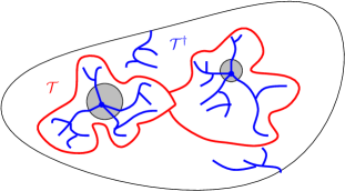
Figure 4: A non-Temperleyan CRSF (in blue). The surface $M$ is the “pair of pants”: a domain of the plane with two holes (in grey in the picture). In this example, $\mathcal{T}$ does not contain any cycle, and hence any connected component flows to the boundary of $M$. Its dual $\mathcal{T}^{\dagger}$ must contain a component with two cycles which overlap: the cycles go around each of the two holes, and must touch each other, as otherwise there would have to be a path in $\mathcal{T}$ separating them, but this is impossible as such as path would have to connect two distinct boundary points. So $\mathcal{T}$ is not Temperleyan. Note that $2g+b=3>2$ here. See Lemma 3.5 for a more general argument.

Temperleyan forests also come with a natural law, which is simply the law of the CRSF conditioned on the event that each component of the dual contains exactly one cycle. We will soon formulate a more explicit criterion for a CRSF $\mathcal{T}$ to be Temperleyan (see Section 3.2 and in particular Theorem 3.6). For now, observe that if $\mathcal{T}$ is a Temperleyan wired oriented CRSF and $\mathcal{T}^{\dagger}$ is its dual, we can assign an orientation to each cycle in each component of $\mathcal{T}^{\dagger}$ arbitrarily from one of the two possible choices. Then we orient all other edges of $\mathcal{T}^{\dagger}$ towards the cycle of that component. We let $\vec{\mathcal{T}}$ be the set of pairs $(t,t^{\dagger})$ where $t$ is a Temperleyan wired oriented CRSF, $t^{\dagger}$ is its dual (hence a free CRSF) for which an orientation of its cycles has been specified, which allows us to view $t^{\dagger}$ also as a free, oriented, CRSF such that each vertex has a single outgoing edge attached to it. Note that if $(t,t^{\dagger})\in\vec{\mathcal{T}}$ then we call $t$ a Temperleyan CRSF and $(t,t^{\dagger})$ a Temperleyan pair or Temperleyan self-dual pair. We hope this terminology will not be too confusing: $t$ is the object we will mostly work with, and $t$ determines $t^{\dagger}$ uniquely up to the orientation of its cycles.

We now state the Temperleyan bijection for general surfaces. Recall that we assign oriented weights $w_{e}$ to each edge $e$ in $\Gamma^{\prime}$, no weight (or unit weight) to edges of $\Gamma^{\dagger}$ and that this turns $G^{\prime}$ into a weighted unoriented graph. Indeed, if $e=(x,y)$ is an oriented edge of $\Gamma^{\prime}$, let $w$ denote the white vertex in the middle of $e$. Then we assign to the unoriented edge $\{x,w\}$ of $G^{\prime}$ the weight $w_{(x,y)}$ and to the edge $\{w,y\}$ of $G^{\prime}$ the weight $w_{(y,x)}$.

For every Temperleyan pair $(t,t^{\dagger})\in\vec{\mathcal{T}}$, we define the measure

$$\operatorname{\mathbb{P}_{Temp}}((\mathcal{T},\mathcal{T}^{\dagger})=(t,t^{\dagger}))=\frac{1}{\operatorname{Z_{Temp}}}1_{\{(t,t^{\dagger})\in\vec{\mathcal{T}}\}}\prod_{e\in t}w(e),$$ (3.1)

where $\operatorname{Z_{Temp}}$ is the partition function.

Theorem 3.3 (Temperleyan bijection on general surfaces).

Let $M,\Gamma^{\prime},(\Gamma^{\dagger})^{\prime},G^{\prime}$ be as in Section 2.3. Then there exists a bijection $\psi$ between $\vec{\mathcal{T}}$ and the set of dimer configurations on $G^{\prime}$. Furthermore if $(\mathcal{T},\mathcal{T}^{\dagger})$ has the law (3.1) then $\textbf{m}=\psi((\mathcal{T},\mathcal{T}^{\dagger}))$ has law (1.1) with unoriented weights on $G^{\prime}$ described above.

We emphasise that it is unclear at this point whether the measure $\operatorname{\mathbb{P}_{Temp}}$ (and consequently the measure on dimers) is not trivially zero as we have only deduced that the construction of $G^{\prime}$ is necessary, but have not deduced that it is sufficient. We prove this later in Proposition 3.4 using a pants decomposition argument.

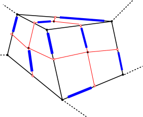
Figure 5: Illustration of the local transformation in Temperley’s bijection. Left: a dimer configuration on a superposition graph. Right: a collection of oriented edges forming dual oriented CRSF.

Proof of Theorem 3.3.

We assume that the set of Temperleyan CRSF and the set of dimer covers are both nonempty (this assumption is validated in Proposition 3.4). Given a Temperleyan pair $(t,t^{\dagger})$, we obtain a configuration of edges $\textbf{m}=\psi((t,t^{\dagger}))$ as follows: for every oriented edge $\vec{e}\in t$ (resp. $\vec{e}\in t^{\dagger}$), we can write $\vec{e}=e_{1}\cup e_{2}$ where $e_{1},e_{2}$ are the first and second halves of $e$ (recall that $e$ is oriented, whether in $t$ or in $t^{\dagger}$), and let $e_{1}\in\textbf{m}$ (see Figure 5). Note that m is a matching on $G^{\prime}$ because every (non boundary) vertex has a unique outgoing edge in either $t$ or $t^{\dagger}$. Furthermore, since $t\cup t^{\dagger}$ spans the black vertices of $G^{\prime}$, the matching is a perfect matching.

Also $\psi$ is injective: if $(t_{1},t_{1}^{\dagger})$ and $(t_{2},t_{2}^{\dagger})$ are two distinct elements of $\vec{\mathcal{T}}$, then there must a black vertex $v$ on $G^{\prime}$ (i.e., a vertex of $\Gamma^{\prime}$ or $(\Gamma^{\dagger})^{\prime}$) such that the unique outgoing edge from $v$ in $t_{1}$ or $t_{1}^{\dagger}$ is different from the unique outgoing edge from $v$ in $t_{2}$ or $t_{2}^{\dagger}$. Hence $v$ will be matched to two distinct white vertices in $\psi((t_{1},t_{1}^{\dagger}))$ and $\psi((t_{2},t_{2}^{\dagger}))$.

We now check $\psi$ is onto. Given a matching m of $G^{\prime}$, we can obtain a pair $(t,t^{\dagger})$ by extending the matched edges: for every nonboundary black vertex $v$ of $G^{\prime}$ (i.e., a vertex of $\Gamma^{\prime}$ or $(\Gamma^{\dagger})^{\prime}$ not on a boundary cycle), let the unique outgoing edge from $v$ be the edge of $\Gamma^{\prime}$ or $(\Gamma^{\dagger})^{\prime}$ containing the white vertex to which $v$ is matched in m. The fact that neither $t$ nor $t^{\dagger}$ contain contractible cycles is the same as in the standard, planar case: if say $t$ has a contractible cycle $C$, then since $\Gamma\setminus C$ has a dimer cover, an elementary counting argument shows that $v-e+f=0$ where $v,e,f$ are the number of vertices, edges and faces of the contractible component $\Gamma\setminus C$. On the other hand, Euler’s formula implies $v-e+f=1$ (again excluding the outer face). Since every vertex $v$ of $t^{\dagger}$ has a unique outgoing edge, $t^{\dagger}$ must have one cycle per component and so $t$ is Temperleyan. This concludes the proof. ∎

3.2 Criterion for a wired CRSF to be Temperleyan

In this Section, we prove the following lemma:

Proposition 3.4.

The graph $G^{\prime}$ obtained in Section 2.3 has a dimer cover. In particular, the measure $\operatorname{\mathbb{P}_{Temp}}$ defined in eq. 3.1 is a probability measure.

As a by product of the proof of Proposition 3.4, we derive a simple criterion for a CRSF to be Temperleyan (Theorem 3.6).

First of all note that if we can find a Temperleyan CRSF of $\Gamma^{\prime}$ then by Theorem 3.3, $G^{\prime}$ has a dimer cover. Next note that if $M$ has the topology of an annulus (with all the nice properties of Section 2.1), then finding a Temperleyan oriented CRSF is straightforward. Indeed, any wired spanning forest in annulus (where both boundaries are wired) is Temperleyan: the dual is a graph containing a single cycle separating the two components touching each boundary. Also notice that for a torus, every oriented CRSF is Temperleyan [19]: essentially an oriented CRSF must contain a cycle (since there is no boundary on a torus) and cutting along this cycle gives us a (bounded) cylinder or equivalently an annulus. The converse is also obviously true when we do not remove edges:

Lemma 3.5.

Let $M$ be nice with $g$ handles and $b$ boundary components and $\Gamma,\Gamma^{\dagger},G$ be embedded as above (i.e. without punctures). A wired Temperleyan oriented CRSF of $\Gamma$ exists if and only if $M$ has the topology of either a torus or an annulus. Furthermore in these cases, all oriented CRSF are Temperleyan.

Proof.

This is simply a consequence of the extended Tempereley’s bijection (Theorem 3.3), because a Temperleyan oriented CRSF and an oriented dual correspond to a dimer configuration (by endowing each cycle with arbitrary orientation and orienting every other edge towards the unique cycle of its component). However, a dimer configuration only exists if and only if $\chi=0$ or equivalently $2g+b=2$ (as discussed in Section 3.1). This equation has only two feasible solutions: $g=1,b=0$ (i.e. a torus) and $g=0,b=2$ (i.e. an annulus). The last part was already argued above the statement. ∎

Proof of Proposition 3.4.

In light of Lemma 3.5, we assume $M$ is neither a torus, nor an annulus. Now recall the pants decomposition [21]: every topological surface of genus $g$ with $b$ boundary components can be decomposed as a finite union of $k=2g+b-2$ pairs of pants. That is, we can find continuous paths on $M$ forming simple noncontractible cycles, so that if we cut open $M$ along these cycles, each component is homeomorphic to a pair of pants. Without loss of generality we can assume that these paths consist of edges from $\Gamma^{\prime}$: indeed, any maximal collection of simple closed curves which are disjoint, pairwise non-homotopic as well as non-homotopic to a boundary component is a suitable collection of such paths (Theorem 9.7.1 in [31]). Clearly, the restriction of $\Gamma^{\prime}$ and $(\Gamma^{\dagger})^{\prime}$ to each such component can be viewed as a pair of dual graphs embedded in a manifold with the topology of a pair of pants where boundary components coming from a cut are described by a single boundary cycle in $\Gamma^{\prime}$. Removing these boundary cycles and the attached half-edges results in a pair of dual graphs faithfully embedded on the pair of pants, exactly as described in Section 2.3 (in particular, each boundary component is now associated with a boundary cycle in $(\Gamma^{\dagger})^{\prime}$ and the boundary condition remains ‘wired’ for $\Gamma$).

Furthermore, since ${\sf k}=2g+b-2$ is also the number of white monomers (punctures) which we remove to get $G^{\prime}$, we can assume without loss of generality that there is exactly one white vertex removed from each component having the topology of the pair of pants, and that such a vertex does not belong to the boundary of $\Gamma$ restricted to that component.

We now claim it suffices to prove Proposition 3.4 when $M$ has the topology of a pair of pants. Indeed, for each cycle arising in the pants decomposition, we fix an arbitrary orientation of this cycle. This defines as in Theorem 3.3 a dimer configuration on the edges of the cycle. Recall that the complement of these cycles define faithfully embedded dual graphs in a number of pair of pants. In each such pair of pants $P$, we superpose a dimer configuration on the graph $G^{\prime}$ restricted to $P$. Superposing these dimer configurations in each pair of pants and on the separating cycles gives rise to a dimer configuration on the whole graph $G^{\prime}$: note that there are no conflicts on the separating cycles, since when we removed these cycles to obtain the pair of pants we also removed the half edges attached to them, so these will never be occupied by dimers.

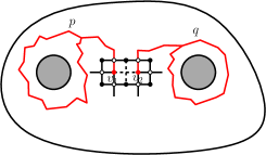
Figure 6: An illustration of the proof of Proposition 3.4 for a pair of pants. The skeleton consists of $p$ and $q$, which decompose the surface into a number of disconnected annuli: three in the first case, two in the second. The dotted edges are the ones removed from $G$ to get $G^{\prime}$.

We thus now assume that $M$ is a pair of pants with a pair of dual graphs faithfully embedded onto it as described in Section 2.3. Let $v_{1}$ and $v_{2}$ be the two vertices of $\Gamma^{\prime}$ which are in the octagon formed because of the removal of white vertex and its attached half-edges. Now consider two disjoint oriented paths $p$ and $q$ in $\Gamma^{\prime}$ starting from $v_{1}$ and $v_{2}$ forming a cycle around two boundaries as shown in Figure 6. If we cut along the loop formed by the paths $p,q$ and the octagon, we get three annuli with faithfully embedded dual graphs (note again that removing the cycles formed by the paths $p$ and $q$ and the attached half-edges means that the each boundary component in the resulting annuli is associated to a boundary cycle in $(\Gamma^{\dagger})^{\prime}$, as in Section 2.3). Thus, by fixing an orientation of $p,q$ and introducing a matching as before, we are back to the annulus case. This we have dealt before in Lemma 3.5, and hence the proof of Proposition 3.4 is complete. ∎

We now deduce from the above an extremely convenient criterion for a wired oriented CRSF to be Temperleyan. Let us supopse $M$ is not the torus or an annulus, whence ${\sf k}=2g+b-2>0$ (we already know that every CRSF is Temperleyan otherwise). Define the branch starting from a primal vertex $v$ of $\Gamma^{\prime}$ to be the path obtained by going along the unique outgoing edge from each vertex (which necessarily ends when a loop is formed or a boundary is hit). Recall that, at a puncture (i.e., a white monomer), there are exactly two vertices $u_{i},v_{i}$ of $\Gamma^{\prime}$ on either side of the puncture. Let $\mathfrak{B}_{i1},\mathfrak{B}_{i2}$ be the branches in $\Gamma^{\prime}$ of $u_{i},v_{i}$ for $1\leq i\leq{\sf k}=2g+b-2$. We call the union of these branches, together with the removed edges $e_{i}$, the skeleton $\mathfrak{s}$ of $\mathcal{T}$. That is,

$$\mathfrak{s}=\bigcup_{i=1}^{\sf k}(\mathfrak{B}_{i1}\cup e_{i}\cup\mathfrak{B}_{i2}).$$

Simply put, the skeleton of $\mathcal{T}$ is the union of the branches emanating out of the punctures.

Theorem 3.6.

Suppose $M$ is not a torus. A wired oriented CRSF is Temperleyan if and only if every component of $M\setminus\mathfrak{s}$ has the topology of an annulus.

(Of course, in the case of an annulus, as already noted there are no punctures and so $\mathfrak{s}=\emptyset$, so the condition is automatically satisfied, as we already know.) The criterion for a CRSF to be Temperleyan is thus just to say that the skeleton cuts the surface into disjoint annuli. Figure 6 gives two examples on a surface $M$ (the ‘pair of pants’) where $M\setminus\mathfrak{s}$ consists of topological annuli (three annuli in the first example, and two in the second example). In the companion paper [5] we denote this conditioning event by $\mathcal{A}_{\mathcal{M}}$. A Temperleyan forest may thus be viewed as a CRSF conditioned on the topological condition $\mathcal{A}_{\mathcal{M}}$, which is asymptotically degenerate (i.e., the probability of $\mathcal{A}_{\mathcal{M}}$ for a wired CRSF tends to zero as the mesh size $\delta$ tends to zero).

Proof.

First note that a component can only have the topology of a torus if the manifold is a torus in which case there is nothing to prove by Lemma 3.5.

For the general case, let $\mathcal{T}$ be a Temperleyan CRSF and let $\mathcal{T}^{\dagger}$ be its dual with a choice of orientation. Note that the vertices (in $G^{\prime}$) of $\mathfrak{s}$ are all matched with each other in the dimer configuration associated to $(\mathcal{T},\mathcal{T}^{\dagger})$. Therefore in each component of $M\setminus\mathfrak{s}$, all vertices are also matched with each other. By Lemma 3.5, this implies that these components are annuli.

Conversely, note that by definition $\mathcal{T}^{\dagger}$ cannot cross $\mathfrak{s}$, and so $\mathcal{T}$ can be restricted to each component of $M\setminus\mathfrak{s}$ to form a wired CRSF. By the other implication in Lemma 3.5, it follows that $\mathcal{T}$ is Temperleyan in each such component and so is globally Temperleyan. ∎

The significance of this criterion is as follows. By Theorem 3.6, a Temperleyan forest can be thought of as a wired CRSF conditioned on the event in the statement of that proposition. However, wired CRSF are easier objects to understand owing to the fact that they can be sampled through a version of Wilson’s algorithm, as will be recalled in Section 3.3.

3.3 Wilson’s algorithm to generate wired oriented CRSF

Recall the measure $\operatorname{\mathbb{P}_{Temp}}$, i.e., the law of $(\mathcal{T},\mathcal{T}^{\dagger})$ on $\vec{\mathcal{T}}$ under the measure eq. 3.1. We will not study directly $\operatorname{\mathbb{P}_{Temp}}$ but rather a measure on $\vec{\mathcal{T}}$ which can be sampled through Wilson’s algorithm and is defined as follows: we first sample a wired oriented CRSF of $\Gamma$ with law

$$\operatorname{\mathbb{P}_{Wils}}(\mathcal{T}=t)=\frac{1}{\operatorname{Z_{Wils}}}1_{\{t\text{ Temperleyan}\}}\prod_{e\in t}w(e);$$

and given $\mathcal{T}=t$, we pick $\mathcal{T}^{\dagger}$ an oriented dual uniformly among all possibilities of orientation of the dual. Thus $\operatorname{\mathbb{P}_{Wils}}$ can be viewed also (with a small abuse of notation) as a mesure on $\vec{\mathcal{T}}$.

The two laws look similar but are in fact different due to the fact that any cycle of the dual $t^{\dagger}$ of a Temperleyan oriented CRSF $t$ can be oriented in two possible ways to determine a dual pair $(t,t^{\dagger})\in\vec{\mathcal{T}}$. We deduce the following relationship:

Lemma 3.7.

Let $(t,t^{\dagger})$ be a Temperleyan wired oriented CRSF such that $t^{\dagger}$ contains exactly $k^{\dagger}$ noncontractible cycles. Then the Radon–Nikodym derivative satisfies

$$\frac{d\operatorname{\mathbb{P}_{Temp}}}{d\operatorname{\mathbb{P}_{Wils}}}(t,t^{\dagger})=\frac{\operatorname{Z_{Wils}}}{\operatorname{Z_{Temp}}}2^{k^{\dagger}}$$

In particular, conditioned on having $k^{\dagger}$ noncontractible cycles for the dual forest, the law $\operatorname{\mathbb{P}_{Temp}}$ and $\operatorname{\mathbb{P}_{Wils}}$ coincide.

Let $\Gamma,\Gamma^{\dagger}$ be faithfully embedded on a nice Riemann surface $M$. We now describe Wilson’s algorithm to generate a wired (but not necessarily Temperleyan) oriented CRSF on $\Gamma$. We prescribe an ordering of the vertices $(v_{0},v_{1},\ldots)$ of $\Gamma$.

• We start from $v_{0}$ and perform a loop-erased random walk until a noncontractible cycle is created or a boundary vertex (i.e., a vertex in $\partial\Gamma$) is hit.

• We start from the next vertex in the ordering which is not included in what we sampled so far and start a loop-erased random walk from it. We stop if we create a noncontractible cycle or hit the part of vertices we have sampled before.

There is a natural orientation of the subgraph created since from every non-boundary vertex there is exactly one outgoing edge through which the loop erased walk exits a vertex after visiting it. Let $\operatorname{\tilde{\mathbb{P}}_{Wils}}$ be the law of the resulting wired oriented CRSF.

Proposition 3.8.

We have

$$\operatorname{\tilde{\mathbb{P}}_{Wils}}(t)=\frac{1}{\operatorname{\tilde{Z}_{Wils}}}\prod_{e\in t}w(e).$$ (3.2)

In particular, $\operatorname{\tilde{\mathbb{P}}_{Wils}}$ generates a wired oriented CRSF of $\Gamma$ as described by Definition 3.1 with law given by (3.2). Furthermore, conditionally on being Temperleyan, $\operatorname{\tilde{\mathbb{P}}_{Wils}}$ coincides with the first marginal of $\operatorname{\mathbb{P}_{Wils}}$.

Proof.

This follows from Theorem 1 and Remark 2 of Kassel–Kenyon [23]. ∎

4 Winding and height function

In this section, we explain the connection between winding of the Temperleyan forest and height function. In order to account for the curvature of the surface it will be important to work on the universal cover and the lifts of both the dimer configuation and the Temperleyan CRSF to it. This will also have the advantage that the dimer height one-form (defined properly below) becomes an actual function on the faces of the lift of the Temperleyan graph embedded on the surface. We refer the reader to Sections 2.4, 2.5 and 2.6 for relevant definitions and notations. The theory we develop below is similar to [27] but with a few important modifications, related in particular to the fact that the Temperleyan forest is typically not connected. See also [35] for a version on the torus.

Recall that $\tilde{M}=\mathbb{C}$ only for the case of the flat torus in this article. We recall the notation $G^{\prime}$ for a Temperleyan graph embedded in $M$ and also recall $\Gamma^{\prime},(\Gamma^{\dagger})^{\prime}$. Now we need to lift the graph $G^{\prime}$ and define a height function which is consistent with this lift.

At this point, we need to spare a few words related to the removal of white vertices from the graph $G$ to obtain a graph with a dimer cover. This operation can be interpreted as inserting certain discrete version of magnetic operators on the free field (e.g. in the sense of [18]). If we want to interpret the height function as winding, the height function would be additively multivalued where it picks up an additional $\pm 2\pi$ winding when it goes around a removed white vertex. This motivates us to introduce a puncture corresponding to each face obtained by removal of a white vertex (cf. Figure 2) and call the new manifold $M^{\prime}$. Recall that we assume each of the punctures converge to fixed distinct points in the manifold (Section 2.3). We now treat every face with a puncture as an outer face.

We lift $G^{\prime}$ to the universal cover $\tilde{M}^{\prime}$ of $M^{\prime}$ and call it $\tilde{G}^{\prime}$. Note that the lift of every non-outer face of $G^{\prime}$ is a quadrangle. For every face $f$ of $\tilde{G}^{\prime}$, we fix once and for all a diagonal $d(f)$ joining the two black vertices. We assume without loss of generality that the diagonal is a smooth curve lying completely inside the quadrangle.

We take a dimer configuration of $G^{\prime}$ which corresponds to a dimer configuration on $\tilde{G}^{\prime}$. We now wish to relate the dimer height function to the winding of a wired oriented CRSF branch adjacent to a path joining the faces, up to certain explicit terms describing the effect of jumping from one component of the CRSF to another. In [27], this connection was established for trees with straight line embeddings in the simply connected case. In [35], the toroidal case was treated, but with only straight line embeddings. In what follows, we need to define the height function properly not necessarily for just straight line embeddings, but for any arbitrary embedding which is smooth except at the vertices. We also need to deal with the fact that the CRSF might have many connected components. The main result of this section, which summarises the desired relationship is stated in Theorem 4.10.

4.1 Winding field of embedded trees and choice of reference flow

To describe properly the connection between winding field of trees and height function of dimers, one needs to get past certain technicalities. One technicality with this connection is that the height function is defined on the faces of the graph and the winding should ideally be computed between vertices of the spanning forest. Another issue we have is that now we need to deal with a spanning forest, and hence the winding between vertices belonging to different connected components must be properly defined. Finally, the definitions should ideally be symmetric with respect to the primal and dual trees.

In this subsection, we temporarily forget about dimers and Temperleyan forests, and focus on how to compute the winding field of a deterministic, infinite, one-ended, spanning tree and its dual tree which are embedded smoothly in the complex plane. This will create a simple setup for connecting dimer height function with winding of Temperleyan spanning trees. Hence the rest of this subsection could be read independently of the rest of the paper.

Consider an infinite one-ended tree $\mathcal{T}$ embedded in $\mathbb{C}$ with the edges embedded smoothly (although having points of non-differentiability at the vertices, which we call corners, are allowed, so that the branches are only piecewise smooth). Recall that the intrinsic winding of any finite branch in this tree is well-defined. Since the infinite tree is one-ended, we can orient the tree towards that unique end. From every vertex $x$ on the tree, we can define an infinite branch $\gamma_{x}$ from $x$ to infinity. Suppose for now

$$|W_{\text{{int}}}(\gamma_{x})|<\infty\text{ for all }x\in\mathcal{T}.$$ (4.1)

Then we can define a winding field $\{h_{\mathcal{T}}(x):x\in\mathcal{T}\}$ of the tree to be simply $h_{\mathcal{T}}(x):=W_{\text{{int}}}(\gamma_{x})$. The following elementary lemma expresses the height in a way which later allows us to extend the definition of $h_{\mathcal{T}}$ even if (4.1) is not satisfied. If $x\notin\gamma_{y}$ and $y\notin\gamma_{x}$, notice that $\gamma_{x}$ and $\gamma_{y}$ eventually merge and $\gamma_{y}$ merges either to the right or to the left of $\gamma_{x}$ (since the tree is embedded in $\mathbb{C}$, this makes sense). Let $\gamma_{xy}$ be the unique path connecting $x$ and $y$ in $\mathcal{T}$.

Lemma 4.1.

In the above setup, if $\gamma_{y}$ merges with $\gamma_{x}$ to its right then

$$h_{\mathcal{T}}(x)-h_{\mathcal{T}}(y)=W_{\text{{int}}}(\gamma_{xy})+\pi$$

If $\gamma_{y}$ merges with $\gamma_{x}$ to its left, then

$$h_{\mathcal{T}}(x)-h_{\mathcal{T}}(y)=W_{\text{{int}}}(\gamma_{xy})-\pi.$$

If $y\in\gamma_{x}$ and $y$ is not a corner (or $x\in\gamma(y)$ and $x$ is not a corner), then

$$h_{\mathcal{T}}(x)-h_{\mathcal{T}}(y)=W_{\text{{int}}}(\gamma_{xy}).$$

Proof.

Notice that the last assertion follows simply from additivity of intrinsic winding. Indeed, for example if $y\in\gamma_{x}$, there is no discontinuity of intrinsic winding at $y$ since $y$ is not a corner.

For the rest, take $m\in\gamma_{x}\cap\gamma_{y}$. Notice that by additivity of winding,

$$h_{\mathcal{T}}(x)-h_{\mathcal{T}}(y) =W_{\text{{int}}}(\gamma_{xm})-W_{\text{{int}}}(\gamma_{ym})$$

$$=W_{\text{{int}}}(\gamma_{xm})+W_{\text{{int}}}(\gamma_{my})$$

$$=W_{\text{{int}}}(\gamma_{xy})+\varepsilon\pi$$

where $\varepsilon=+1$ (or $\varepsilon=-1$) if $\gamma_{y}$ merge with $\gamma_{x}$ to its right (or left). This is clear since we need to do a half turn to move from $\gamma_{xm}$ to $\gamma_{my}$ at $m$ and the turn is clockwise if $\gamma_{y}$ merges to the right of $\gamma_{x}$ and anticlockwise otherwise. ∎

We remark that the last assertion of the above lemma works even at corners by adding the appropriate angle at the corner to match the winding field difference. In what follows, we avoid using winding field at corners, hence this ambiguity would not bother us. We also remark that such a definition easily extends to a finite tree with the branches oriented towards a fixed vertex in the tree in place of being oriented towards “infinity”. Finally the formula for $h(x)-h(y)$ described in Lemma 4.1 can be taken to be the definition of the winding field (or rather its gradient) for any tree embedded with piecewise smooth edges, even if (4.1) is not satisfied. This will be the typical situation for our setup.

We will now extend the definition of the winding field of $\mathcal{T}$ to the faces of a graph spanned by $\mathcal{T}$. For context, we remind the reader that in Section 3.1, a bijection between Temperleyan CRSF and dimer configurations was established. Also recall that the height function of a dimer configuration is defined on the faces of the graph. Thus it is necessary to do this extension carefully so that the dimer height differences become exactly the same as the winding field, perhaps up to some global topological error term coming from the jumps between various components in the forest.

With this in mind, take an infinite locally finite graph $\Gamma$ embedded smoothly in $\mathbb{C}$, except perhaps at the vertices where we might have corners and let $\mathcal{T}$ be a one ended spanning tree of $\Gamma$ (we emphasise that we are still considering a spanning tree for the moment and not yet a forest). Therefore the dual spanning tree $\mathcal{T}^{\dagger}$ of the dual graph $\Gamma^{\dagger}$ is also one-ended. Let $G$ be the superposition graph (in $\mathbb{C}$), as introduced in Section 2.3 (the appropriate infinite version of the graph $G$ there). It will be useful to augment the trees $\mathcal{T}$ and $\mathcal{T}^{\dagger}$ to include diagonals, as follows. We fix a point on the diagonal $d(f)$ once and for all, which we denote by $m(f)$ and sometimes refer to as midpoint of the diagonal by an abuse of terminology. For each face, add to $\mathcal{T}$ (resp. $\mathcal{T}^{\dagger}$) the portion of the diagonal $d(f)$ connecting the point $m(f)$ to the unique primal (dual) vertex touching $d(f)$. This way the primal and dual trees meet in each face $f$ at the (smooth) point $m(f)$ on the diagonal $d(f)$ of that face. With a small abuse of notation, we will still denote $\mathcal{T}$ and $\mathcal{T}^{\dagger}$ these augmented trees.

Note that we can orient $\mathcal{T},\mathcal{T}^{\dagger}$ towards their unique ends. This allows us to define two winding fields as above (one for $\mathcal{T}$ and one for $\mathcal{T}^{\dagger}$). Having oriented $\mathcal{T}$ and $\mathcal{T}^{\dagger}$ we can also apply the local operation of Figure 5 as described in Section 3.1 to obtain a dimer matching of $G$ (recall that for the moment $\mathcal{T}$ and $\mathcal{T}^{\dagger}$ are still a dual pair of spanning trees, not forests). We will first need to define a suitable reference flow on $G$, which will then allow us to speak of the height function associated to the dimer configuration and then show the relation between this dimer height function and the two above winding fields.

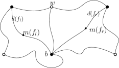
Figure 7: The definition of the height function in terms of winding.

Definition 4.2 (reference flow).

Let $w,b$ be two adjacent white and black vertices and let $f_{l},f_{r}$ be the faces to the left and right of the oriented edge $(bw)$. Define

$$\omega_{ref}(wb)=\frac{1}{2\pi}(W_{\text{{int}}}((m(f_{r}),b)\cup(b,m(f_{l})))+\pi)$$ (4.2)

where $(m(f_{l}),b)$ is the portion of $d(f_{l})$ joining $m(f_{l})$ and $b$, and similarly $(m(f_{r}),b)$. Define $\omega_{ref}(bw)=-\omega_{ref}(wb)$ (see Figure 7).

Figure 8: Proof of Lemma 4.3.

Lemma 4.3.

$\omega_{ref}$ defined above is a valid reference flow. That is, the total mass sent out of any white vertex $w$, $\sum_{b\sim w}\omega_{ref}(wb)$, is equal to one; and the total mass received to any black vertex $b$, $\sum_{w\sim b}\omega_{ref}(wb)$, is also one.

Proof.

Let $w$ be a white vertex. Notice that in $\sum_{b\sim w}\omega_{ref}(wb)$, the oriented diagonals form a clockwise loop whose total winding is $-2\pi$. Adding $+\pi$ for each of the surrounding black vertices, and dividing by $2\pi$, we see that the total flow out of $w$ is indeed 1 as desired.

For a black vertex $b$, the argument is better explained by considering a picture (see Figure 8). Fatten the “star” formed by the half-diagonals incident to $b$ into a star shaped domain. Then notice that the total flow out of $b$ is simply the limit of the total winding, divided by $2\pi$, of the boundary of this domain (again in the clockwise orientation this time), as the domain thins into the “star”. Indeed, the $-\pi$ term in the definition of $\omega_{ref}$ in (4.2) counts the half-turn as we move from the left side to the right side of a half-diagonal. Since the total winding of such a curve is $-2\pi$, it follows that the total flow out of $b$ is $-1$, as desired. ∎

We are now ready to relate the three notions of height function defined by the pair of dual spanning trees $\mathcal{T},\mathcal{T}^{\dagger}$. To do so, note that we can extend the definition of the winding field of both $\mathcal{T}$ and $\mathcal{T}^{\dagger}$ from Lemma 4.1 to the augmented trees.

Proposition 4.4.

In the above setup, let $h_{\mathcal{T}}$ and $h_{\mathcal{T}^{\dagger}}$ be the winding field of $\mathcal{T}$ and $\mathcal{T}^{\dagger}$ respectively. Let $h_{\dim}$ be the height function corresponding to the dimer configuration obtained from $(\mathcal{T},\mathcal{T}^{\dagger})$ with reference flow $\omega_{ref}$. For any two faces $f,f^{\prime}$,

$$h_{\mathcal{T}}(m(f^{\prime}))-h_{\mathcal{T}}(m(f))=h_{\mathcal{T}^{\dagger}}(m(f^{\prime}))-h_{\mathcal{T}^{\dagger}}(m(f))=2\pi(h_{\dim}(f^{\prime})-h_{\dim}(f)).$$

Remark 4.5.

Note that having augmented the trees as explained above, the winding fields in $\mathcal{T}$ and $\mathcal{T}^{\dagger}$ now play a completely symmetric role.

Proof.

Define $\gamma_{v}$ for the branch of $\mathcal{T}$ starting from $v$ and similarly define $\gamma^{\dagger}_{v}$. For a face $f$, we define $\gamma_{f}$ (respectively $\gamma^{\dagger}_{f}$) to be the branch of the augmented tree $\mathcal{T}$ (resp. $\mathcal{T}^{\dagger}$) starting from $m(f)$. Fix faces $f$ and $f^{\prime}$ and assume without loss of generality that $\gamma_{f^{\prime}}$ is to the right of $\gamma_{f}$. Note that this means that $\gamma^{\dagger}_{f^{\prime}}$ is to the left of $\gamma^{\dagger}_{f}$. Also note that

$$W_{\text{{int}}}(\gamma_{ff^{\prime}})+W_{\text{{int}}}(\gamma^{\dagger}_{f^{\prime}f})=-2\pi$$

because $\gamma_{ff^{\prime}}$ concatenated with $\gamma^{\dagger}_{f^{\prime}f}$ forms a clockwise loop and there is no jump at $m(f)$ and $m(f^{\prime})$ because by assumption the midpoint $m(f)$ is a smooth point of $d(f)$. The first equality easily follows by applying the definition of winding field from Lemma 4.1.

For the last equality let $f_{l},f_{r}$ be adjacent faces. Let the common (oriented) edge be $(bw)$ with $b$ being the black and $w$ the white vertex and let $f_{r}$ lie to its right. We assume without loss of generality that $b$ is a primal vertex. From the definition of $\omega_{ref}$ and recalling the sign convention of the flow defining the height function (Section 2.4)

$$2\pi(h_{\dim}(f_{r})-h_{\dim}(f_{l})) =\omega_{ref}(wb)-2\pi 1_{\text{$(bw)$ occupied by dimer}}$$

$$=W_{\text{{int}}}((f_{r},b)\cup(b,f_{l}))+\pi-2\pi 1_{\text{$(bw)$ occupied by dimer}}$$

Note that that $\gamma_{f_{r}}$ and $\gamma_{f_{l}}$ merge at $b$. Also note from Temperleyan bijection that if $(bw)$ is occupied by a dimer, then $\gamma_{b}$ starts by using the (half) edge $bw$ which implies that $\gamma_{f_{l}}$ lies to the left of $\gamma_{f_{r}}$. Otherwise, $\gamma_{f_{l}}$ lies to the left of $\gamma_{f_{r}}$. We conclude using the definition of winding field from Lemma 4.1 and the above equation. ∎

As a step towards extending the correspondence of Proposition 4.4 to forests, we now explain how to read off the height change along a path in the graph which does not necessarily follow the tree branches. Note that although the dimer height function is independent of the chosen path, it is not clear how to see this path independence looking at just the winding field. For an arbitrary path in the graph, there could be several “jumps” over edges in the dual tree and it turns out that these jumps contribute an extra $\pm\pi$ on top of the winding, depending on orientation. It will turn out that in case of forests, there is an analogous contribution for jumping over dual components which separate the primal connected components (and vice-versa).

Figure 9: The path $P$ in $\Gamma$ is the union of solid blue and dashed blue edges. Here number of partitions $k=3$. The solid blue denotes the segments in the tree $\mathcal{T}$. The union of solid red and solid blue edges is the modified path. The orange dotted paths denote the direction in which the primal tree goes off to $\infty$ and the green dotted path denotes the same for the dual tree. This determines the $\varepsilon_{i}^{\prime}s$ and $\delta_{i}^{\prime}$s. Here $\varepsilon_{1}=-1,\varepsilon_{2}=1,\varepsilon_{3}=-1$ and $\delta_{1}=1,\delta_{2}=-1$.

Let $P$ be a self avoiding path in $\Gamma$. We can partition this path into segments belonging to $\mathcal{T}$ separated by edges not belonging to $\mathcal{T}$ (we remind the reader that $\mathcal{T}$ is still a tree, not yet a forest). Let us call these segments $(P_{1},\ldots,P_{k})$ and let $(e_{1},\ldots,e_{k-1})$ be the edges in $\Gamma$ separating them. Note that we allow $P_{i}$ to be a single vertex. Let $(x_{i},y_{i})$ be the starting and ending points of $P_{i}$.

Now we modify $P_{i}$ as follows. Observe that the oriented edge $(y_{i},x_{i+1})$ has two faces of $G$ to its left. Call the one incident to $y_{i}$, $f_{i}^{-}$ and the one incident to $x_{i+1}$, $f_{i}^{+}$. Call $m_{i}^{-},m_{i}^{+}$ the midpoint of the diagonals of these faces. We pick a face incident to $x_{1}$ and $y_{k}$ and add the segments joining these vertices and the midpoint of their diagonals. Call these endpoints $m_{0}^{+},m_{k}^{-}$ respectively. We also join $y_{i}$ to $x_{i+1}$ using the diagonal segments of $f_{i}^{-}$ and $f_{i}^{+}$. Finally we delete the edges $e_{i}$. This completes the modification of the path $P$, which we are still going to denote as $P$ (see Figure 9).

We also partition $P$ into segments as $[m_{i}^{+},m_{i+1}^{-}]$ for $0\leq i\leq k-1$ and $[m_{i}^{-},m_{i}^{+}]$ for $1\leq i\leq k-1$. Let $\varepsilon_{i}=+1$ (resp. $-1$) if $\gamma_{m_{i}^{-}}$ lies to the right (resp. left) of $\gamma_{m_{i-1}^{+}}$ for $1\leq i\leq k$. Let $\delta_{i}=+1$ (resp. $-1$) if $\gamma^{\dagger}_{m_{i}^{+}}$ lies to the right (resp. left) of $\gamma^{\dagger}_{m_{i}^{-}}$ for $1\leq i\leq k-1$.

Lemma 4.6.

Under the above setup,

$$h_{\mathcal{T}}(m_{0}^{+})-h_{\mathcal{T}}(m_{k}^{-})=W_{\text{{int}}}(P)+\pi(\sum_{i=1}^{k}\varepsilon_{i}+\sum_{i=1}^{k-1}\delta_{i})=2\pi(h_{\dim}(f_{1})-h_{\dim}(f_{k}))$$

Proof.

By summing along each segment, the first equalty is simply a consequence of the definition and additivity of $h_{\mathcal{T}}$ and Proposition 4.4. The second equality is also an implication of the second equality of Proposition 4.4. ∎

Extension to forests.

We now extend the definition of winding field to forests before relating it to a dimer height function. Suppose $\mathcal{T}$ is now a spanning forest of $\Gamma$ where each component is infinite. Let $\mathcal{T}^{\dagger}$ be its dual, and note that its components are also necessarily infinite, and it is also a forest. We fix an end of each component of primal and dual, and orient the trees towards that end. Thus we obtain an oriented pair of dual forests. Note again that by the local operation of Temperleyan bijection, we can find a dimer configuration on the superposition graph $G$ corresponding to $(\mathcal{T},\mathcal{T}^{\dagger})$. Let $h_{\dim}$ be the dimer height function corresponding to this dimer configuration with reference flow given by $\omega_{ref}$ defined in Definition 4.2.

We augment $(\mathcal{T},\mathcal{T}^{\dagger})$ in the same way as in the connected case: in each face join the midpoint of the diagonals to the corresponding primal vertices in $\mathcal{T}$ and dual vertices in $\mathcal{T}^{\dagger}$.

Definition 4.7.

In the above setup, define the winding field of $(\mathcal{T},\mathcal{T}^{\dagger})$ to be the same as that given by the first equality of the formula in Lemma 4.6. This is well defined up to a global shift by $\mathbb{R}$.

Notice that in the definition of $\delta_{i}$ above (the error term we need to add when “jumping” over a dual edge) is defined using the dual tree, and hence there is no issue of connectivity when dealing with spanning forests rather than spanning trees. It is straightforward to see that the above notion of winding field for forests is well-defined as the second equality of Lemma 4.6 also tells us that this quantity is the same as the dimer height function (up to a global shift), and in particular is independent of the path $P$. The proof of Lemma 4.6 relies on additivity of winding for each edge and does not depend on the fact that $(\mathcal{T},\mathcal{T}^{\dagger})$ is a tree–dual tree pair and not a forest.

Remark 4.8.

Note that there is no assumption about the number of ends of $(\mathcal{T},\mathcal{T}^{\dagger})$ in the above definition: it makes sense as long as an orientation is fixed towards a unique end in each component. Later we will see that because of toplogical reasons, each component (either of primal or dual) of the relevant (random) lift of the Temperleyan forests we need to deal with has exactly two ends almost surely. This leaves us with a choice of which end to orient for each connected component, and once this choice is fixed, the above definition can be applied to define the winding field, which is going to be equal to the dimer height function (up to a global shift). But since the above definition for general forests with arbitrary ends require no additional extra effort, we decided to keep this definition.

4.2 Winding of CRSF and height function

In this section, we show how to extend the connection between winding and height function (established in [27]) from the simply connected setting in the Euclidean plane with straight line embeddings to height one forms on general surfaces. Firstly we work in the universal cover if the surface, so that the CRSF is lifted to a spanning forest for which we have already worked out the connection in the previous section. However there are many ways to choose a path between vertices in different components. Most of the work in this section will actually be to specify a convenient one so that the winding computation is as simple as possible.

Recall $\Gamma,\Gamma^{\dagger}$ from Section 2.3. We call the vertices in the lift of $(\Gamma^{\dagger})^{\prime}$ the dual vertices and those in the lift of $\Gamma^{\prime}$ primal vertices. Recall that the dual of a wired Temperleyan CRSF of $\Gamma^{\prime}$ is a free CRSF of $(\Gamma^{\dagger})^{\prime}$. In this setup, the punctures are mapped to the boundary of the disc. Furthermore, each component of both the wired Temperleyan CRSF and its dual contains either a single cycle or contains a boundary component. In the rest of this section we drop the adjective Temperleyan and refer simply to the wired and free CRSF.

Roughly this choice of path is as follows. As a preparatory step, we first observe that the cycles in the CRSF, when lifted, become bi-infinite paths, which we call spines. Next we show in Lemma 4.9 that:

• In the hyperbolic case, the spines converge to some point on the boundary of the hyperbolic disc (i.e., on the unit circle),

• In the parabolic case of the torus, the spines converge to infinity in some fixed asymptotic direction.

We could not find a soft probabilistic argument for this and had to rely on tools coming from the classical theory of Riemann surfaces (essentially, uniformisation and Fuchsian theory). We will postpone the proof of Lemma 4.9 to the appendix in order to maintain the flow in the paper. Armed with Lemma 4.9, given $x$ and $y$, we choose the path between them as follows. Suppose we are in the hyperbolic case. We first move from $x$ along the spine of its tree component to infinity and do the same for $y$. These paths converge to the unit circle at $\zeta_{x},\zeta_{y}$. We join $\zeta_{x},\zeta_{y}$ along an arc on the unit circle (there are two choices of this arc, and a canonical choice is possible). This defines a path and we prove in Theorem 4.10 that the height gap between $x$ and $y$ can be written as the winding of this path plus a sum of terms of the form $\pm\pi$ depending on the “jumps” over the primal and dual spines lying in between. Note that this is a non-trivial fact as the path is not completely in the graph, but “goes through infinity”. An analogous path is chosen in the torus by choosing points along the corresponding spines in place of $\zeta_{x},\zeta_{y}$ and then taking a limit. This choice is particularly useful as we do not need to compute the winding coming from the components lying in between trees containing $x$ and $y$, which would be hard to keep track of using Wilson’s algorithm.

Figure 10: The conformal maps between an annulus and its universal cover. The dotted lines separate different copies of the fundamental domain. The blue and red curves show two loops in the surface and the associated spines in the cover.

When relating the height function to winding, it is convenient to replace each boundary vertex of $\partial\Gamma$ by a cycle surrounding the corresponding hole in the surface. In this manner, all paths of the wired CRSF that end up in the boundary can also be considered to form loops – call this also a boundary loop in what follows. Hence all components of both the wired and free CRSF can be viewed as a set of paths flowing towards a single noncontractible cycle.

It is clear from the unique path lifting property that each oriented loop in the CRSF (including any “boundary loop” mentioned above, if there is any) corresponds to a bi-infinite simple path in the lift (the one obtained by going along the loop infinitely many times in clockwise and anti-clockwise direction). We call this a spine. Note also that each loop corresponds in the lift to multiple spines (except in the case of the annulus). We now state a useful lemma about the geometry of spines.

Lemma 4.9.

Assume $M$ is hyperbolic. Any spine $S$ in the CRSF is either a simple path in $\mathbb{D}$ connecting two points in $\partial\mathbb{D}$ or a simple loop containing a unique point in $\partial\mathbb{D}$.

The proof of Lemma 4.9 uses classical tools from the theory of Riemann surfaces, so we postpone to appendix A in order to not disrupt the rest of the argument too much.

Lemma 4.9 allows us to describe the geometry of spines and dual spines. In the case of the torus, it is clear that spines and dual spines form alternating bi-infinite paths, all in the same asymptotic direction. When the universal cover is the disc, each (oriented) spine separates $\mathbb{D}$ into two simply connected components which lie to its right and left. Given two spines $S$ and $S^{\prime}$, we have a well defined region $\Omega_{S,S^{\prime}}$ between them which is bounded by $S$, $S^{\prime}$ and two portions of $\partial\mathbb{D}$ (if $S$ and $S^{\prime}$ are loops, then these portions of $\partial\mathbb{D}$ are understood as only prime ends associated with the same point). We say that a spine or dual spine $S^{\prime\prime}$ separates $S$ from $S^{\prime}$ if it connects these two portions of $\partial\mathbb{D}$. Since the graph $\tilde{G}^{\prime}$ only has accumulation points on $\partial\mathbb{D}$, it is easy to see that two spines can only be separated by finitely many others. Furthermore, two adjacent dual spines must be separated by a primal spine.

Figure 11: An illustration of spines in the hyperbolic case. The spines $S$ and $S^{\prime}$ are separated by a dual spine drawn in dashed blue. This spine also separates $S^{\prime\prime}$ and $S^{\prime}$ (left). The second and third figures from the left illustrate the choice of $\varepsilon_{S}$ in Theorem 4.10: in the second, $\varepsilon_{S}=1=-\varepsilon_{S^{\prime}}$. In the third figure (note that the orientation of $S^{\prime}$ is reversed), $\varepsilon_{S}=\varepsilon_{S^{\prime}}=1$.

Let us call the lifts also $(\mathcal{T},\mathcal{T}^{\dagger})$ with an abuse of notation. Also augment these trees by joining the midpoint of the diagonals to the respective endpoints, as explained in Section 4.1. Now pick two faces $f,f^{\prime}$ and let $S,S^{\prime}$ be the spines of the components of $\mathcal{T}$ containing $m(f),m(f^{\prime})$. Let $\Omega_{S,S^{\prime}}$ be the component between them as above. Draw a simple curve connecting $S$ and $S^{\prime}$ in $\Omega_{S,S^{\prime}}$, and oriented from $S$ to $S^{\prime}$. For each primal spine $\sigma\subset\Omega_{S,S^{\prime}}$ (hence not including $S$ and $S^{\prime}$), let $\varepsilon_{\sigma}$ be the algebraic number of times $\sigma$ is crossed by this curve (with the convention of counting +1 if $\sigma$ is crossed from its left to its right by the curve and -1 otherwise). If $\sigma$ is not crossed, define $\varepsilon_{\sigma}$ to be 0. Define $\delta_{\sigma}$ similarly for primal spines. Notice that

$$\sum_{\sigma\subset\Omega_{S,S^{\prime}}}\varepsilon_{\sigma}+\delta_{\sigma}$$ (4.3)

is a topological term which does not depend on the choice of the curve (where the sum is over all primal and dual spines contained in $\Omega_{S,S^{\prime}})$. Also, its only dependence on $f$ and $f^{\prime}$ is through the spines $S$ and $S^{\prime}$.

We will need a slightly modified definition of $\varepsilon_{S}$ and $\varepsilon_{S^{\prime}}$. For any face $f$, let $\gamma_{f}$ be the infinite oriented path in $\mathcal{T}$ started from $m(f)$ and going off to infinity along the unique outgoing oriented edges. Let $\zeta$ be the limit point of $\gamma_{f}$ (which exists due to Lemma 4.9). Let $\zeta^{\prime}$ be the limiting endpoint of $S^{\prime}$ which lies in the same connected component of $\partial\tilde{M}\cap\Omega_{S,S^{\prime}}$ as $\zeta$. Note that we are not defining $\zeta^{\prime}$ to be the limit point of $\gamma_{f^{\prime}}$ as it could be the case that $\zeta$ and $\zeta^{\prime}$ might lie in different boundary components of $\partial\tilde{M}\cap\Omega_{S,S^{\prime}}$ (depending on the orientation of $S^{\prime}$). In case $S,S^{\prime}$ are loops through the same boundary point, we want $\zeta$ and $\zeta^{\prime}$ to be in the same prime end of $\Omega_{S,S^{\prime}}$.

Now we define $\varepsilon_{S}$ and $\varepsilon_{S^{\prime}}$. Define $\varepsilon_{S}=+1$. Now we have a few cases for $\varepsilon_{S^{\prime}}$.

• If the limit point of $\gamma_{f^{\prime}}$ lies in the same component of $\partial\tilde{M}\cap\Omega_{S,S^{\prime}}$, then define $\varepsilon_{S^{\prime}}=1$.

• If not, the there are two cases. If $f^{\prime}$ lies in $\Omega_{S,S^{\prime}}$, then define $\varepsilon_{S^{\prime}}=-1$. Otherwise, define $\varepsilon_{S^{\prime}}=+1$.

The above choice of $\varepsilon_{S},\varepsilon_{S^{\prime}}$ is made in accordance with Lemma 4.6. Indeed imagine a path not going through infinity, but which starts at $f$ moves up along the spine $S$ in the direction of its orientation, joins two vertices in $S,S^{\prime}$ very close to the boundary arc and then moves down along $S^{\prime}$ (either in the direction of the orientation of $S^{\prime}$ or the opposite, depending on the orientation of $S^{\prime}$ itself). Note that for this path, the choice of the $\varepsilon_{S},\varepsilon_{S^{\prime}}$ exactly matches with the choice defined for Lemma 4.6. We refer the readers to the second figure of Figure 11 for the case when the limit point of $\gamma_{f^{\prime}}$ does not lie in the same component of $\partial\tilde{M}\cap\Omega_{S,S^{\prime}}$ and $f^{\prime}$ lies in $\Omega_{S,S^{\prime}}$, in which case $\varepsilon_{S^{\prime}}=-1$.

Let $(\zeta,\zeta^{\prime})$ be the arc joining $\zeta$ and $\zeta^{\prime}$ (which could be a single point in case $\zeta=\zeta^{\prime}$) in $\partial\tilde{M}$ in the hyperbolic case. Let $h_{\dim}$ be the dimer configuration corresponding to the pair $(\mathcal{T},\mathcal{T}^{\dagger})$ with reference flow given by Definition 4.2. We can now state the following final result relating the dimer height function to the winding of trees in the general setting we consider:

Theorem 4.10.

In the hyperbolic case, let $\gamma:=\gamma_{f,f^{\prime}}$ be the curve formed by concatenating $\gamma_{f}$, $(\zeta,\zeta^{\prime})$ and the path in $\mathcal{T}$ joining $\zeta^{\prime}$ to $m(f^{\prime})$. Orient $\gamma$ from $m(f)$ to $m(f^{\prime})$. We have the following deterministic relation:

$$h_{\dim}(f^{\prime})-h_{\dim}(f)=W(\gamma,m(f))+W(\gamma,m(f^{\prime}))+\pi\sum_{\sigma\in\bar{\Omega}_{S,S^{\prime}}}(\varepsilon_{\sigma}+\delta_{\sigma})$$ (4.4)

Here the sum $\sum_{\sigma\in\bar{\Omega}_{S,S^{\prime}}}\varepsilon_{\sigma}+\delta_{\sigma}$ is as in (4.3) but also includes $S$ and $S^{\prime}$.

Remark 4.11.

The same statement holds in the case of the torus, but with a few obvious modifications, where we think of $\zeta$ and $\zeta^{\prime}$ being the same point at infinity (so starting from $f$ and $f^{\prime}$ both paths go to infinity in the same direction). Then (4.4) is also true but obviously without the winding term between $\zeta$ and $\zeta^{\prime}$.

Proof.

Consider the winding field $h$ corresponding to $(\mathcal{T},\mathcal{T}^{\dagger})$ defined as in Lemma 4.6. See also the discussion following that lemma for the definition when $\mathcal{T}$ is a forest. Notice that the winding field differences between the diagonal midpoints are exactly the dimer height differences between the corresponding faces, hence it is enough to prove the lemma for the winding field.

Let us consider the hyperbolic case first. Take two vertices $x,x^{\prime}$ in $S,S^{\prime}$ respectively. Observe that we can find a path joining $x,x^{\prime}$ which goes along the primal components, and moves from one component to the other by “jumping” over dual spines (i.e. going along edges whose dual belong to a dual spine). Also one can make sure that the path is minimal, in the sense that every component between those of $x,x^{\prime}$ (i.e. components which separate $S,S^{\prime}$) is visited at most once. Call this path $(x,x^{\prime})$. Now letting $x\to\zeta$ and $x^{\prime}\to\zeta^{\prime}$, we can also ensure that the portion of $\Omega_{S,S^{\prime}}$ bounded by $(x,x^{\prime}),(\zeta,\zeta^{\prime})$ and the spines $S,S^{\prime}$ contains none of $f$ or $f^{\prime}$.

Let $\tilde{\gamma}$ be the path obtained by concatenating $(m(f),x),(x,x^{\prime}),(x^{\prime},m(f^{\prime}))$. From Lemma 4.6, it is clear that

$$h_{\dim}(f^{\prime})-h_{\dim}(f)=W_{\text{{int}}}(\tilde{\gamma})+\pi\sum_{S}(\varepsilon_{S}+\delta_{S})$$

Indeed, notice that since the path is minimal, the $\varepsilon_{S},\delta_{S}$ terms are defined so as to match with the definition of $\varepsilon_{i},\delta_{i}$ in Lemma 4.6. Furthermore, $W_{\text{{int}}}(\tilde{\gamma})=W_{\text{{int}}}(\gamma)$ because of the above choice of $x,x^{\prime}$. We finish the proof using Lemma 2.7.

For the torus case, the same proof applies by noticing that $W((x,x^{\prime}),m(f))+W((x,x^{\prime}),m(f^{\prime}))$ converges to 0 as $x$ and $x^{\prime}$ go to infinity along $S,S^{\prime}$ in the same asymptotic direction.

Finally, the fact that the term $\pi\sum_{S}(\varepsilon_{S}+\delta_{S})$ converges follows simply from the fact that the number of noncontractible components is a.s. finite in the limiting CRSF (and hence so is the number of spines which separate $S,S^{\prime}$ into different components). ∎

4.3 Convergence of Instanton component

We now prove a lemma about the instanton component of the height one-form which shows that it is a function of only the noncontractible loops and nothing else. Although this may be intuitively clear, it is not so easy to see using the connection between height difference and winding established in Theorem 4.10. Indeed, consider a noncontractible (continuous) closed curve $\lambda$ in the manifold. To compute the height gap we first lift $\lambda$ to the cover $p^{-1}(\lambda)$ and we then compute the height gap between two copies of the starting point of the loop. A priori this might depend on the winding of the spines corresponding to the start and end points of $p^{-1}(\lambda)$. However, it is clear in the case of the torus that the winding terms cancel out as the spines of the starting and ending points are translates of each other. It turns out the same is true in the hyperbolic case but a slightly more involved argument is needed, as the map from one fundamental domain to another is not just a translation but a Möbius map which perturbs the winding. Thus, the proof of the following lemma requires this input from Riemannian geometry and the assumptions on the graph in Section 2.3, so we encourage the reader to read the introduction of appendix A and Section 2.3 before reading this proof.

Take an ordered finite set of continuous simple loops which forms the basis of the first homology group of $M^{\prime}$, all endowed with a fixed orientation. Let $\mathsf{H}$ be the finite set of numbers which denote the height change along these loops. It is well-known (see Theorem 2.5) that $\mathfrak{h}$ is completely determined by $\mathsf{H}$ (at the discrete level). In the following lemma, we write a superscript $\delta$ to account for the dependance in $\delta$ as in Section 2.3.

Lemma 4.12.

Let $(\mathfrak{C}^{\#\delta},(\mathfrak{C}^{\dagger})^{\#\delta})$ be the set of oriented noncontractible loops of the primal and dual Temperlayen CRSF. Let $\mathfrak{h}^{\#\delta}$ be the instanton component of the height 1-form of the dimer configuration corresponding to this CRSF pair given by the extended Temperley bijection. Then $\mathfrak{h}^{\#\delta}$ is a function of $(\mathfrak{C}^{\#\delta},(\mathfrak{C}^{\dagger})^{\#\delta})$ only.

Furthermore, $\mathsf{H}^{\#\delta}$ also converges and the limit is measurable with respect to the limit of $(\mathfrak{C}^{\#\delta},(\mathfrak{C}^{\dagger})^{\#\delta})$ as $\delta\to 0$.

Proof.

Using the main result of the companion paper [5, Theorem 1.2], we know that the Temperleyan forest converges in Schramm topology, in particular, the skeleton converges. Therefore the measurability part is clear once we show that $\mathfrak{h}^{\#\delta}$ is a function of $(\mathfrak{C}^{\#\delta},(\mathfrak{C}^{\dagger})^{\#\delta})$ only.

Take a set of loops which forms the basis of the homology group of $M^{\prime}$. It is enough to prove that the height change along one such loop $\lambda$ is a function of $(\mathfrak{C},\mathfrak{C}^{\dagger})$ only.

Let us first consider the hyperbolic case. Lift the loop to the universal cover and compute the winding between its endpoints using Theorem 4.10 (see Figure 11). Note that it is enough to show that the winding term in Theorem 4.10 depends only on $(\mathfrak{C},\mathfrak{C}^{\dagger})$. To this end, we borrow the notations from Theorem 4.10. We will actually show that the only contribution of the winding term in Theorem 4.10 comes from the winding of the arc $(\zeta,\zeta^{\prime})$. Clearly, the winding of the interval $(\zeta,\zeta^{\prime})$ is determined by the spines and hence $(\mathfrak{C},\mathfrak{C}^{\dagger})$. Using the isomorphism between the Fuchsian group corresponding to $M^{\prime}$ and the fundamental group of $M^{\prime}$, (see appendix A), we see that there exists a Möbius transform $\Phi$ which maps $\gamma_{f}$ to $\gamma_{f^{\prime}}$ and which depends only on the loop $\lambda$. In the hyperbolic case, observe that a Möbius map extends slightly beyond the unit disc and so it makes sense to talk about $\Phi^{\prime}(\zeta)$. Using Lemma 2.8, we see that the difference in winding between $\gamma_{f}$ and $\gamma_{f^{\prime}}$ is $\arg_{\Phi^{\prime}(\tilde{M}^{\prime})}(\Phi^{\prime}(\zeta))-\arg_{\Phi^{\prime}(\tilde{M}^{\prime})}(\Phi^{\prime}(m(f)))$ which is completely determined by $(\mathfrak{C},\mathfrak{C}^{\dagger})$.

In the toroidal case, as mentioned before, the mapping $\Phi$ is simply a translation (i.e. $\Phi^{\prime}$ is a constant), so the lemma is immediate using the same argument as above. This completes the proof. ∎

The next lemma, combined with Lemma 4.12, shows in a precise sense that the instanton component converges in law (see also Remark 6.15).

Lemma 4.13.

In the setting of Section 2.3, suppose $x,y\in\tilde{M}^{\prime}$ and that $f,f^{\prime}$ are two faces closest to $x,y$ (breaking ties arbitrarily). Then $\sum_{\sigma\in\bar{\Omega}_{S,S^{\prime}}}(\varepsilon_{\sigma}+\delta_{\sigma})$ converges in law. In fact, this convergence in law holds jointly for an arbitrary number of pairs of faces approximating given points in $\tilde{M}^{\prime}$.

Proof.

By [5, Theorem 1.2], the Temperleyan forest $\mathcal{T}^{\#\delta}$ converges to a continuum limit $\mathcal{T}$ (under the assumptions of this theorem). Consequently the nontrivial primal and dual cycles $(\mathfrak{C},\mathfrak{C}^{\dagger})$ also converge (with respect to the Hausdorff metric) to the nontrivial cycles induced by $\mathcal{T}$. Moreover, since the number $K$ of nontrivial cycles has superexponential tail as shown in the companion paper [5], no two cycles are likely to be close to one another by Wilson’s algorithm and the crossing assumption. It is easy to deduce that $\sum_{S}(\varepsilon_{S}+\delta_{S})$ converges and the limit is measurable with respect to the limit of $(\mathfrak{C}^{\#\delta},(\mathfrak{C}^{\dagger})^{\#\delta})$. The joint convergence for an arbitrary finite number of pair of faces also follows in the same manner. ∎

5 Local coupling

In this section we prove a local discrete coupling result which extends ideas of [4] to the setup of Riemann surfaces. Roughly speaking, the goal of such a result is to show that the local geometry in a small neighbourhood of a Temperleyan CRSF is given by that of a uniform spanning tree in the surface or, alternatively (and more usefully), in some reference planar domain. Moreover, locally around a finite number of given points, the configurations can be coupled to independent such USTs.

Recall that the actual Temperleyan CRSF’s cannot be completely sampled using the standard Wilson’s algorithm. However, due to Theorem 3.6, given the skeleton $\mathfrak{s}$ emanating from either side of the punctures, the rest of the Temperleyan CRSF can be sampled from Wilson’s algorithm. The main result in this section is Proposition 5.9.

The argument follows the same line of arguments as in [4] so let us first recall the strategy there. This consists of two main steps. Consider $k$ points $v_{1},\ldots,v_{k}$ in $(\Gamma^{\prime})^{\#\delta}$. In the first step, we choose cutsets at a small but macroscopic distance around each of the $k$ points, such that the cutsets separate the points from each other and from the rest of the graph. We reveal all the branches emanating from these cutsets. This leaves $k$ unexplored subgraphs $\Gamma_{i}^{\#\delta}$, one around each point. In this step the key point is to make sure that the $\Gamma_{i}^{\#\delta}$ are macroscopic (e.g., contain a ball of a radius roughly of the same order of magnitude as the distance to the cutsets). Clearly, the conditional law of the tree in each $\Gamma_{i}^{\#\delta}$ is that of a wired UST. Moreover, these wired USTs are also independent conditionally given the cutset exploration. (Of course, unconditionally there is still some dependence). The second step is then to say that in each $\Gamma_{i}^{\#\delta}$, one can couple a wired UST with a full plane one, which shows, among other things, that the unconditional distribution is close to being independent.

To adapt this strategy to Riemann surfaces, if the $\Gamma_{i}^{\#\delta}$ are sufficiently small so that it is simply connected, then the conditional law of the CRSF in each $\Gamma_{i}^{\#\delta}$ will also be that of a wired UST, so that the second step can be used directly. For the first step however (cutset exploration), we will need to redo parts of the proof to take into account the possible loops in the CRSF.

We first recall two useful lemmas from the companion article ([5, Lemmas 2.5 and 2.6])

Lemma 5.1 (Beurling type estimate).

For all $r,\varepsilon>0$ there exists $\eta>0$ such that for any $\delta<\delta(\eta)$ and for any vertex $v\in\Gamma^{\#\delta}$ such that $\eta/2<d_{M}(v,\partial M)<\eta$, the probability that a simple random walk exits $B_{M}(v,r):=\{z\in M:d_{M}(z,v)<r\}$ before hitting $\partial\Gamma^{\#\delta}$ is at most $\varepsilon$.

Lemma 5.2.

Let $K_{0}\subset K^{\prime}_{0}\subset M$ be open connected sets and let $K\subset K_{0}^{\prime},K^{\prime}$ be compact sets which are the closures of $K_{0},K^{\prime}_{0}$. Also assume $K$ contains a loop which is noncontractible in $M$. Then there exists a $\delta_{K,K^{\prime}}>0$ and $\alpha_{K,K^{\prime}}>0$ depending only on $K,K^{\prime}$ such that for all $\delta<\delta_{K,K^{\prime}}$ and all $v\in\Gamma^{\#\delta}$ such that $v\in K$, simple random walk started from $v$ has probability at least $\alpha_{K,K^{\prime}}$ of forming a noncontractible loop before exiting $K^{\prime}$.

5.1 Cutset exploration

We now describe the construction more precisely. Fix $k$ points $v_{1},\ldots,v_{k}$ in $(\Gamma^{\prime})^{\#\delta}$ and let $N_{v_{i}}$ be small enough neighbourhoods around each $v_{i}$ such that $\{N_{v_{i}}\}_{1\leq i\leq k}$ do not intersect each other or the pre-specified boundary $\partial\Gamma^{\#\delta}$ of $\Gamma^{\#\delta}$ (if the boundary is non-empty) and for each $1\leq i\leq k$, $p^{-1}(N_{v_{i}})$ is a disjoint union of sets in $\tilde{M}$ such that $p$ restricted to each component is a homeomorphism to its image. Also for each $i$, fix one pre-image $\tilde{v}_{i}$ of $v_{i}$ and let $\tilde{N}_{\tilde{v}_{i}}$ denote the component of $\tilde{v_{i}}$ in $p^{-1}(N_{v_{i}})$. Let $R(\tilde{v}_{i},\tilde{N}_{\tilde{v}_{i}})$ be the inradius seen from $\tilde{v}_{i}$ in $\tilde{M}$ with respect to the Euclidean metric, and call

$$r=\min_{1\leq i\leq k}R(\tilde{v}_{i};\tilde{N}_{\tilde{v}_{i}}).$$ (5.1)

(We point out that in our setup it is natural to define these quantities with respect to Euclidean geometry on $\tilde{M}$ and project to $M$, because our assumption and in particular the uniform crossing condition are stated with respect to this geometry; whereas the intrinsic geometry of $M$ does not really appear in our setup).

We denote by $B_{\textsf{euc}}(\tilde{v},r)$ the Euclidean ball of radius $r$ around $\tilde{v}$ and for $r^{\prime}>r$, let $A_{\textsf{euc}}(\tilde{v},r,r^{\prime})=B_{\textsf{euc}}(\tilde{v},r^{\prime})\setminus B_{\textsf{euc}}(\tilde{v},r)$ be the Euclidean annulus of inradius $r$ and outer radius $r^{\prime}$. Let $H_{i}$ be a set of vertices in $p(A_{\textsf{euc}}(\tilde{v}_{i},r/2,r))\cap(\Gamma^{\prime})^{\#\delta}$ which disconnects $v_{i}$ from $\partial N_{v_{i}}$. The cutset exploration is done in two steps

1. First sample the skeleton according to the correct law (i.e. according to CRSF branches with the global conditioning that the branches divide the manifold into annuli).

2. Then, reveal all the branches from $H_{i},1\leq i\leq k$ using (unconditioned) Wilson’s algorithm, resulting in a subgraph $\mathcal{T}_{H_{i}}^{\#\delta}$, $1\leq i\leq k$.

We say a vertex $v_{j}$ has cutset isolation radius $6^{-k}r$ at scale $r$ if

$$p(B_{\textsf{euc}}(\tilde{v}_{j},6^{-k}r))\text{ does not contain any vertex from $\mathcal{T}_{H_{i}}^{\#\delta}$}.$$

Let us define $J_{v_{j}}$ as the the minimum value such that $v_{j}$ has isolation radius $6^{-J_{v_{j}}}r$ and let $J=\max_{j}J_{v_{j}}$.

We want to show that $J$ has exponential tail (which results in polynomial tail of the isolation radius). To this end, we rely on the following bound on the distance between a loop-erased walk and a point, which is a version of Proposition 4.11 in [4].

Lemma 5.3.

Let $\gamma$ be a loop-erased random walk starting from a vertex $v$ until it hits $(\partial\Gamma^{\prime})^{\#\delta}$ or a noncontractible loop is created. Let $u\neq v$ be another vertex and let $\tilde{u}$ be one of the images under $p^{-1}$ of $u$. Let $r$ be small enough such that $U:=\bar{B}_{\textsf{euc}}(\tilde{u},r)$, is contained in the pre-image of $N_{u}$ which contains $\tilde{u}$. Then there exist constants $\alpha,c>0$ (depending only on the initial assumptions of the graph) such that for all $\delta<\delta_{U}$ and all $n\in(0,\log_{2}(\frac{Cr\delta_{0}}{\delta})-1)$ where $\delta_{U},\delta_{0}$ are as in the crossing condition (assumption iv),

$$\mathbb{P}(\gamma\cap p(B_{\textsf{euc}}(\tilde{u},2^{-n}r))\neq\emptyset)<c\alpha^{n}.$$

Proof.

This is almost identical to Lemma 4.11 in [4] except we now need to take into account the topology as well. To emphasise the differences with Lemma 4.11 in [4], we recall the strategy there. The idea is that if the loop erased walk on the manifold comes inside $p(B_{\textsf{euc}}(\tilde{u},2^{-n}r))$ then some lift of the random walk must necessarily come within $B_{\textsf{euc}}(\tilde{u},2^{-n}r)$ – call this region (exponential) scale $n$. Furthermore, after the last such visit, this (lift of the) random walk must cross $n$ many annuli without making a loop around $\tilde{u}$ (which we called a “full turn”). This has a probability bounded by $e^{-cn}$.

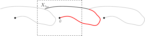
Figure 12: A schematic representation (in solid line) of the lift of the loop erasure of the random walk on the torus until a noncontractible loop is formed. Call this path $\tilde{\gamma}$ and let $\gamma=p(\tilde{\gamma})$. The dashed square denotes the fundamental domain and the dashed paths denote some other lifts of $\gamma$. In this case, $\tilde{\gamma}$ stops inside the fundamental domain.

In the current situation however, the random walk might form a noncontractible loop before exiting $U$, and therefore its relevant lift described above does not necessarily have to cross $n$ many annuli (see e.g. Figure 12) after coming within Euclidean distance $2^{-n}r$ of $\tilde{u}$ before we stop it. Thus we cannot simply apply the argument of the previous paper. We overcome this using the following idea which we first explain informally. The random walk on the manifold may visit $p(B_{\textsf{euc}}(\tilde{u},r))$ multiple times. Consider one such time when it enters $p(B_{\textsf{euc}}(\tilde{u},r))$ (not necessarily the first time) and suppose its relevant lift $\tilde{X}$ which also enters $B_{\textsf{euc}}(\tilde{u},r)$ at that time. Let $X^{\prime}$ be the portion of the loop-erasure of $X$ on $M$ at that time such that, if the random walk hits $X^{\prime}$ later on, then a noncontractible loop in $M$ is formed. Assume that $X^{\prime}$ comes inside $p(B_{\textsf{euc}}(\tilde{u},2^{-m}r))$. In order for the whole loop-erasure $\gamma$ to come inside $p(B_{\textsf{euc}}(\tilde{u},2^{-n}r))$ the following events must take place on one such visit. First, the lift $\tilde{X}$ has to cross the first $m$ scales without performing a full turn (otherwise it would close a noncontractible loop on the manifold and stop); this has a probability bounded by $e^{-cm}$. Then $\tilde{X}$ needs to come within Euclidean distance $2^{-n}r$ of $\tilde{u}$, but we bound crudely the probability of this event by 1. Finally $\tilde{X}$ needs to come back out after the last visit to $B_{\textsf{euc}}(\tilde{u},2^{-n}r)$ in such a way that no full turn occurs between distances $2^{-n}r$ and $2^{-m}r$ (for the same reason as in the simply connected case). The probability of this event can be bounded by $e^{-c(n-m)}$. The intersection of these three events gives the right overall upper bound: $e^{-cm}e^{-c(n-m)}=e^{-cn}$.

Let us fill in the details. Let $C_{i}$ be the Euclidean circle of radius $r_{i}:=2^{-i}r$ around $\tilde{u}$ for $i\geq 0$. We start a random walk $X$ from $v$ (to emphasise again: $X$ is on the manifold $M$). Let $\{\tau_{k}\}$ be a sequence of stopping times defined inductively as follows. Set $\tau_{0}=0$. Having defined $\tau_{k}$ to be a time when the random walk $X$ crosses or hits some circle $p(C_{i(k)})$, define $\tau_{k+1}$ to be the smallest time after $\tau_{k}$ when the random walk crosses or hits either $p(C_{i(k)-1})$ or $p(C_{i(k)+1})$; this defines $\tau_{k}$ by induction for every $k\geq 1$. If $i(k)=0$, define $\tau_{k+1}$ to be the smallest time after $\tau_{k}$ when the random walk crosses or hits $p(C_{i(k)+1})$. Let $k_{\text{exit}}$ be the smallest integer such that in the interval $[\tau_{k_{\text{exit}}},\tau_{k_{\text{exit}}+1}]$ either a noncontractible loop is created by the loop-erasure of the random walk or the random walk hits the boundary $\partial\Gamma^{\#\delta}$. Let $\kappa_{0},\kappa_{1},\ldots,\kappa_{N}$ be the set of indices $k<k_{\text{exit}}+1$ when $X_{\tau_{k}}$ has crossed or hit $p(C_{0})$. Also note that the portions $X[\tau_{\kappa_{0}+1},\tau_{\kappa_{1}}]$, $X[\tau_{\kappa_{1}+1},\tau_{\kappa_{2}}],\ldots$ are contained inside $p(C_{0})$; while the portions $X[\tau_{\kappa_{0}},\tau_{\kappa_{0}+1}],X[\tau_{\kappa_{1}},\tau_{\kappa_{1}+1}],\ldots$ are contained outside $p(C_{1})$. Our first claim is that $N$ has exponential tail, i.e., $\exists\alpha_{1}\in(0,1)$, such that for all $n\geq 1$,

$$\mathbb{P}(N>n)<\alpha_{1}^{n}.$$ (5.2)

Indeed, using Lemma 5.2, every time the walk hits $p(C_{0})$, there is a positive probability independent of the past that the walk creates a noncontractible loop before returning to $p(C_{1})$. Therefore, $N$ has geometric tail. This proves (5.2).

Let $\mathcal{S}$ be the set of points $\{X(\tau_{k})\}_{k\geq 1}$. Note that given $\mathcal{S}$, the pieces of random walk $\{X[\tau_{k},\tau_{k+1}]\}$ are independent of each other. We call such pieces elementary pieces of the walk. If $i(k)\neq 0$, $X[\tau_{k},\tau_{k+1}]$ is (given $\mathcal{S}$) a random walk starting from $X_{\tau_{k}}$ conditioned to exit the annulus $p(A_{\textsf{euc}}(\tilde{u},r_{i(k)-1},r_{i(k)+1}))$ at $X_{\tau_{k+1}}$. If $i(k)=0$, $X[\tau_{k},\tau_{k+1}]$ is a random walk which is conditioned to next hit $p(B_{\textsf{euc}}(\tilde{u},r/2))$ at $X_{\tau_{k+1}}$. (Note that this property is lost if we solely condition on $\{X(\tau_{k})\}_{k\leq\kappa_{N}}$ since the conditioning on $N$ is complicated.) By Lemma 4.7 in [4], conditionally on $\mathcal{S}$, each random walk piece $X[\tau_{k},\tau_{k+1}]$ has a uniformly positive probability to do a full turn in the annulus $p(A_{\textsf{euc}}(\tilde{u},r_{i(k)-1},r_{i(k)}))$ for $\delta\leq\delta_{U}$ and given range of $n$ (where $\delta_{U}$ comes from the uniform crossing assumption). Here we define a full turn to be the event that the random walk crosses every curve joining the inner and outer boundary in the specified annulus. Indeed, although Lemma 4.7 in [4] gives the uniform positive probability estimate for crossing in the Euclidean plane, the estimate is valid here by considering the relevant lift of $X[\tau_{k},\tau_{k+1}]$ which is inside $\bar{B}_{\textsf{euc}}(\tilde{u},r)=U$ and applying the uniform crossing estimate in the universal cover. Let us also point out that $\delta$ is chosen small enough so that the uniform crossing estimate is valid inside $U$.

We now define certain low probability events $\mathsf{E}_{1},\ldots,\mathsf{E}_{n}$ such that one of them must take place if the loop-erasure of $X$ is to enter $B_{n}:=p(B_{\textsf{euc}}(\tilde{u},2^{-n}r))$. Let us condition on $\mathcal{S}$. We say the event $\mathsf{E}_{j}$ occurs if:

1. The portion $X[\tau_{\kappa_{j-1}+1},\tau_{\kappa_{j}}]$ intersects $B_{n}$. We then let $\lambda_{j}$ be the smallest $k$ in $[\tau_{\kappa_{j-1}+1},\tau_{\kappa_{j}}]$ such that $X_{\tau_{k}}$ crosses (or hits) $p(C_{n})$.

2. Let $X_{j}^{\prime}$ be the portion of the loop-erasure of $X[0,\tau_{\kappa_{j-1}+1}]$ such that if the walk $X[\tau_{\kappa_{j-1}+1},\tau_{\kappa_{j}}]$ intersects $X_{j}^{\prime}$, a noncontractible loop would be created. Let $m$ be the maximum index such that $X^{\prime}$ intersects the circle $p(C_{m})$.

   Then for the event $\mathsf{E}_{j}$ to hold we also require, in addition to the previous point, that: for any $\kappa_{j-1}+1\leq k\leq\lambda_{j}$ if $i(k)<m$, then the walk $X[\tau_{k},\tau_{k+1}]$ does not perform a full turn in $p(A_{\textsf{euc}}(\tilde{u},r_{i(k)-1},r_{i(k)}))$. If no such $m$ exists (e.g., if $X_{j}^{\prime}$ is empty), we do not require anything further.

3. Let $\ell_{j}$ be the last $k$ before $\kappa_{j}$ such that $X_{\tau_{k}}$ crosses (or hits) $p(C_{n})$. Let $\ell^{\prime}_{j}$ be the first time after $\ell_{j}$ that the walk intersects $p(C_{m+1}).$ Then in addition to the previous two points, for $\mathsf{E}_{j}$ to hold we require that the walk $X[\tau_{k},\tau_{k+1}]$ does not perform a full turn for any $\ell_{j}\leq k\leq\ell_{j}^{\prime}$.

From the discussion above, it is clear that we have the following lemma.

Lemma 5.4.

We have

$$\{\gamma\cap B_{n}\neq\emptyset\}\subseteq\{N\leq n,\cup_{j=1}^{n}\mathsf{E}_{j}\}\cup\{N>n\}.$$

Thus all we need to show is that the event on the right hand side of Lemma 5.4 has exponential tail bound. Now we claim that

$$\mathbb{P}(\mathsf{E}_{j}|\mathcal{S})\leq e^{-c^{\prime}n}\text{ and so }\mathbb{P}(\mathsf{E}_{j})\leq e^{-c^{\prime}n}.$$

This is justified using the uniform positive probability of the walk $X$ performing a full turn, even conditionally given $\mathcal{S}$. Indeed, conditioned on $\mathcal{S}$, we have that the event (ii) in the definition of $\mathsf{E}_{j}$ has probability at most $e^{-c^{\prime}m}$, and conditioned on event in (ii), the event in (iii) has probability at most $e^{-c^{\prime\prime}(n-m)}$ since conditionally given $\mathcal{S}$, the random walk portions $X[\tau_{k},\tau_{k+1}]$ are independent. Thus the overall probability given $\mathcal{S}$ is at most $e^{-cn}$ with $c=c^{\prime}\wedge c^{\prime\prime}$. All in all, using eq. 5.2, Lemma 5.4 and a union bound, we obtain

$$\mathbb{P}(\{\gamma\cap B_{n}\neq\emptyset\})\leq ne^{-c^{\prime}n}+e^{-c^{\prime}n}\leq ce^{-c^{\prime}n}.$$

thereby concluding the proof. ∎

Lemma 5.5.

Let $\mathfrak{s}$ denote the skeleton. Let $u$ be a vertex which is not one of the punctures and let $\tilde{u}$ be one of the images under $p^{-1}$ of $u$. Let $s$ be small enough such that $U:=\bar{B}_{\textsf{euc}}(\tilde{u},s)$, is contained in the pre-image of $N_{u}$ which contains $\tilde{u}$. Then there exist constants $\alpha,c>0$ (depending only on the initial assumptions of the graph) such that for all $\delta<\delta_{U}$ and all $n\in(0,\log_{2}(\frac{Cs\delta_{0}}{\delta})-1)$ where $\delta_{U},\delta_{0}$ are as in the crossing condition (assumption iv),

$$\mathbb{P}(\mathfrak{s}\cap p(B_{\textsf{euc}}(\tilde{u},2^{-n}s))\neq\emptyset)<c\alpha^{n}.$$

Proof.

This follows from [5, Proposition 6.5] and Lemma 5.3.

Let us explain why this Proposition implies the desired statement in the case ${\sf k}=1$. For this we need to introduce a few notations used in [5]. Let $\bar{\lambda}_{\mathcal{M}}$ denote the law $\mathfrak{s}$. Let $\bm{\eta}_{r}=(\eta_{r}^{1},\eta_{r}^{2})$ denote the portion of the branches of the skeleton until they exit a ball of radius $r$ around the puncture, for a very small choice of $r$. For each such path $\eta^{i}_{r}$ (with $i=1,2$) run independent simple random walks from their tips, where each walk is conditioned to exit the ball of radius $r^{\prime}>r$ before hitting $\eta^{i}_{r}$, for another small choice of $r^{\prime}$. After hitting $r^{\prime}$ the walks are allowed to run unconditionally until they either hit $\bm{\eta}_{r}$ or $(\partial\Gamma^{\prime})^{\#\delta}$ or their loop erasure creates a non-contractible loop. Let $\tilde{\mu}_{r,r^{\prime}}$ denote the joint law of the loop erasures of the resulting pair of walks. For any event $E$ which is measurable with respect to $\mathfrak{s}\setminus\bm{\eta}_{r}$, [5, Proposition 6.4] asserts that

$$\underline{\lambda}_{\mathcal{M}}(E)\leq C\left(\sqrt{\sup_{\bm{\eta}_{r/2}}\tilde{\mu}_{r/2,r}(E)+\sup_{\bm{\eta}_{r/4}}\tilde{\mu}_{r/4,r/2}(E)}\right)$$ (5.3)

where the supremum is over all possible $\bm{\eta}_{r/2}$ (resp. $\bm{\eta}_{r/4}$)

It is easy to see using the Markov property of the independent random walks used to sample $\tilde{\mu}_{r/2,r}$ that after hitting $r$, the result of Lemma 5.3 kicks in, yielding the required exponential bound for $\tilde{\mu}_{r/2,r}(E)$. The same argument obviously applies to $\tilde{\mu}_{r/4,r/2}(E)$, yielding the desired statement.

The application of [5, Proposition 6.5] for ${\sf k}>1$ is analogous. We skip the details here. ∎

We now state the result showing an exponential tail of $J$, which is a combination of Lemmas 5.3 and 5.5 and Schramm’s lemma, and is identical to the proof of Lemma 4.20 in [4] (see also the proof of Theorem 4.21 in [4]); as it is identical we skip the proof here.

Lemma 5.6.

There exist constants $c,c^{\prime}>0$ such that the following holds. Let $\tilde{D}$ be a compact set containing $B(\tilde{v}_{i},r)$ for $1\leq i\leq k$ where $r$ is as in (5.1). Then for all $\delta\in(0,\delta_{\tilde{D}})$ and for all $m\in(0,\log_{6}(\delta_{0}r/\delta)-1)$,

$$\mathbb{P}(J>m)\leq ce^{-c^{\prime}m}.$$

Finally, we state a lemma which says that with exponentially high probability, a branch of the CRSF, after entering an exponential scale $t$ does not backtrack to a smaller scale. Such a lemma for SLE curves can be found in [33] (see also Lemma 3.4 in [4] in the simply connected case).

Lemma 5.7.

Fix $u,U,\delta_{U}$ as in Lemma 5.3. Suppose $\gamma$ is the loop-erasure of a simple random walk in $\Gamma^{\#\delta}$ started from vertex $u$ until it hits the boundary or creates a noncontractible loop. Suppose $\tilde{\gamma}$ is the lift of $\gamma$ started from $\tilde{u}$ (parametrised from $\tilde{u}$ to its endpoint). There exist constants $c,c^{\prime}>0$ (depending only on the initial assumptions of the graph) such that for all $\delta<\delta_{U}$ and all $n\in(0,\log_{2}(\frac{Cr\delta_{0}}{\delta})-1)$

$$\mathbb{P}(\text{$\tilde{\gamma}$ enters $B_{\textsf{euc}}(\tilde{u},r2^{-n})$ after exiting $B_{\textsf{euc}}(\tilde{u},r2^{-n/2})$})\leq ce^{-c^{\prime}n}.$$

Proof.

Let $\mathsf{E}$ be the event that $\tilde{\gamma}$ enters $B_{\textsf{euc}}(\tilde{u},r2^{-n})$ after exiting $B_{\textsf{euc}}(\tilde{u},r2^{-n/2})$. Let $r$ be as in Lemma 5.3 and assume $n$ is even without loss of generality. The argument for this is very similar to Lemma 5.3 and in fact simpler, so we content ourselves with a sketch. Let $r,C_{i},B_{i}$ be as in the proof of Lemma 5.3. We look at the lift $\tilde{X}$ of the simple random walk $X$ started at $\tilde{u}$ and we stop when either $X$ hits the boundary or a noncontractible loop is created. Let $\tau_{k}$ be the set of stopping times defined as in the proof of Lemma 5.3 but for the lift $\tilde{X}$ instead of $X$ and let $\mathcal{S}$ be the set $\{\tilde{X}(\tau_{k})\}_{k\geq 1}$. Observe that lift of the loop erasure of $X$ is the loop erasure of $\tilde{X}$ since erasing contractible loops commutes with lifting to the universal cover. If the loop erasure of $\tilde{X}$ has to backtrack to scale $n$, the random walk has to necessarily enter scale $n$ after leaving scale $n/2$. Let $J$ be the largest $j$ such that $\tilde{X}_{\tau_{j}}$ crosses or hits $C_{n}$ after leaving $C_{n/2}$ and let $I$ be the largest index $i$ smaller than $J$ when $\tilde{X}_{\tau_{i}}$ crosses or hits $C_{n/2}$. Conditioned on $\mathcal{S}$, if $\mathsf{E}$ occurs, then $\tilde{X}$ enters $B_{n}$ at least once after leaving $B_{n/2}$, and none of the elementary pieces of the walk between $\tau_{I}$ and $\tau_{J}$ can perform a full turn. But again, conditioned on $\mathcal{S}$ there is a uniformly positive probability to do a full turn for each elementary piece. Since there are at least $n/4$ such elementary pieces contained in $[\tau_{I},\tau_{J}]$, we conclude the proof of the lemma applying the upper bound on the full-turn estimate on each elementary piece. ∎

5.2 Full coupling

The results of the previous section covered the first step in the proof of the coupling. As we mentioned above, the second step is identical to the simply connected case so we only recall the main statements.

We first recall the result which we will need from [4]. We use the notations and assumptions already in force. Let $\tilde{D}\subset\tilde{D}^{\prime}\subset\tilde{M}^{\prime}$ be two simply connected compact domains and fix $\tilde{v}\in\tilde{D}^{\#\delta}$. Let $\mathcal{T}^{\tilde{D}^{\prime}},\mathcal{T}^{\tilde{D}}$ denote the wired UST respectively in $(\tilde{D}^{\prime})^{\#\delta}$ and $\tilde{D}^{\#\delta}$. Let $r_{\tilde{v}}$ denote $R(\tilde{v},\tilde{N}_{\tilde{v}})$ as in eq. 5.1 (the largest Euclidean radius so that $p$ is injective).

Lemma 5.8 (Theorem 4.21, [4]).

There exists $c,c^{\prime}>0$ such that the following holds. Fix $\tilde{v},\tilde{D},\tilde{D}^{\prime}$ as above. There exists a coupling between $\mathcal{T}^{\tilde{D}}$ and $\mathcal{T}^{\tilde{D}^{\prime}}$ and a random variable $R^{\prime}>0$ such that

$$\mathcal{T}^{\tilde{D}^{\prime}}\cap{B_{\textsf{euc}}(\tilde{v},R^{\prime})^{\#\delta}}=\mathcal{T}^{\tilde{D}}\cap{B_{\textsf{euc}}(\tilde{v},R^{\prime})^{\#\delta}}.$$

Furthermore, for all $\delta<\delta_{\tilde{D}^{\prime}}$ and for all $m\in(0,\log_{6}(\delta_{0}r_{\tilde{v}}/\delta)-1)$, if we write $R^{\prime}=6^{-K_{v}}r_{\tilde{v},\tilde{D}}$ where $r_{\tilde{v},\tilde{D}}$ is the minimum of $r_{\tilde{v}}$ and the Euclidean distance between $\tilde{v}$ and $\partial\tilde{D}$, then

$$\mathbb{P}(K_{v}\geq m)\leq ce^{-c^{\prime}m}.$$

We now put together the cutset exploration with the above one-point coupling from the simply connected case as follows. Recall the notations from Section 5.1. Let $\mathcal{T}_{H_{i}}^{\#\delta}$ be the branches revealed in the cutset exploration around each $v_{i}$. Let $\mathcal{T}_{H}^{\#\delta}=\cup_{i=1}^{k}\mathcal{T}_{H_{i}}^{\#\delta}$. Let $\Gamma_{i}^{\#\delta}$ be the connected component of $(\Gamma^{\prime})^{\#\delta}\setminus\mathcal{T}_{H}^{\#\delta}$ containing $v_{i}$. Observe that given $\mathcal{T}^{\#\delta}_{H}$, the law of $\mathcal{T}^{\#\delta}\cap\Gamma_{i}^{\#\delta}$ are independent wired UST in $\Gamma_{i}^{\#\delta}$ (with the natural boundary), by the generalised Wilson algorithm. Applying the coupling of Lemma 5.8 in the lift of $\Gamma_{i}^{\#\delta}$ to $\tilde{M}^{\prime}$ and some fixed compact $\tilde{D}$ in $\tilde{M}^{\prime}$ containing some lifts $\tilde{v}_{1},\ldots,\tilde{v}_{k}$ of points $v_{1},\ldots,v_{k}$, we obtain a coupling of the oriented CRSF in $\Gamma^{\#\delta}$ and independent wired USTs $(\mathcal{T}^{\tilde{D}}_{i})_{1\leq i\leq k}$ in $\tilde{D}$. Furthermore, the $r$ in (5.1) and $r_{\tilde{v}}$ in Lemma 5.8 differs by a constant multiplicative factor which depends only on the choice of lifts of the vertices. Furthermore, we may (and will) choose the $(\mathcal{T}^{\tilde{D}}_{i})_{1\leq i\leq k}$ to be independent of $\mathcal{T}_{H}^{\#\delta}$. In fact, note that for each $1\leq i\leq k$, $\mathcal{T}^{\tilde{D}}_{i}$ may be chosen independent of the restriction of $\mathcal{T}^{\#\delta}$ to $\cup_{j\neq i}p(B(\tilde{v}_{j},r/2))$.

Proposition 5.9.

The above coupling has the following properties: there exists random variables $R_{1},\ldots,R_{k}$ such that

$$\mathcal{T}^{\#\delta}\cap p(B(\tilde{v}_{i},R_{i}))=p(\mathcal{T}^{\tilde{D}}_{i}\cap B(\tilde{v}_{i},R_{i})).$$ (5.4)

Furthermore if we write $R_{i}=6^{-I_{v_{i}}}r_{i}$ where $r_{i}$ is the minimum of $r$ as in (5.1) and the distance between $\tilde{v}_{i}$ and $\partial\tilde{D}$, then for all $\delta\leq\delta_{\tilde{D}}$, and for all $1\leq i\leq k$, for all $n\in(0,\log_{6}(\delta_{0}r_{i}/\delta)-1)$,

$$\mathbb{P}(I_{v_{i}}\geq n)\leq ce^{-c^{\prime}n}$$ (5.5)

for some constants $c,c^{\prime}>0$ (depending only on the initial assumptions on the graph). In particular, $\mathbb{P}(I_{v_{i}}\geq n)\leq ce^{-c^{\prime}n}\vee\delta^{c^{\prime}}$.

The set of noncontractible loops of $\mathcal{T}^{\#\delta}$ is measurable with respect to $\mathcal{T}_{H}^{\#\delta}$. In particular, $(\mathcal{T}_{i}^{\tilde{D}})_{1\leq i\leq k}$ are also independent of the set of oriented noncontractible loops in the oriented CRSF.

Observe that when $I_{v_{i}}$ is very big or $r_{i}$ is very small, it is possible that the ball $B(v_{i},R_{i})$ is reduced to a point so the statement (5.4) is trivial (that is, (5.4) holds for a single vertex). This happens with a probability which is at most $\delta^{c^{\prime}}$ for some $c^{\prime}$.

Proof.

This follows immediately from Lemma 5.6 and Lemma 5.8 once we observe that $I_{v_{i}}$ is within $O(1)$ of the sum of $J_{v_{i}}$ in Lemma 5.6 and $K_{v_{i}}$ in Lemma 5.8, both of which have exponential tails.

The proof of the final assertion is a topological fact. Indeed, conditioned on $\mathcal{T}_{H}^{\#\delta}$, it is a deterministic fact that none of the oriented noncontractible loops pass through the portion of the CRSF in $\Gamma_{i}^{\#\delta}$ (which is a wired UST). Indeed, otherwise we would have a path joining two points of the wired boundary of a wired UST which is impossible. Thus, the wired UST in each $\Gamma_{i}^{\#\delta}$ is conditionally independent of the noncontractible loops and hence so are $\mathcal{T}_{i}^{\tilde{D}}$s. ∎

6 Convergence of height function and forms

In this section, we precisely state our main result (this is Theorem 6.1) and then prove it. Recalling the sketch from Section 1.3, we see that what remains to be done is to go from the convergence of the Temperleyan CRSF to the convergence of its winding field using the coupling of Section 5. The global idea is the same as in [4] but some of the estimates on winding of LERW have to be redone. The primary difficulty is that spines are made of multiple copies of LERW, and hence Wilson’s algorithm cannot be used to estimate the winding of all the copies. These are dealt with respectively in Sections 6.2 and 6.3. The proof of the main result is finally concluded in Section 6.4.

6.1 Precise statement of the result

We first provide a precise statement of what we prove. From now on, we work with the manifold $M^{\prime}$ which is obtained by removing $2g+b-2$ points from its interior. Recall that the white vertices removed from $G^{\#\delta}$ to obtain a Temperleyan graph in Theorem 3.6 will converge to these points. Denote by $\tilde{M}^{\prime}$ the universal cover of $M^{\prime}$; in the sequel “lift” refers to lift on $\tilde{M}^{\prime}$. Let $h^{\#\delta}_{\mathsf{}}$ be the height function defined as in Section 4 sampled using eq. 1.1. Recall that $h^{{\#\delta}}_{\mathsf{}}$ is a function from the the dual of $(\tilde{G}^{\prime})^{\#\delta}$ to $\mathbb{R}$, that is defined up to a global additive constant and that a choice of reference flow is used in the definition that depends only on the embedding. Recall the probability measures $\operatorname{\mathbb{P}_{Wils}}$ and $\operatorname{\mathbb{P}_{Temp}}$ from Section 3.3.

First, we extend $h^{\#\delta}$ to a function $h^{\#\delta}_{\textsf{ext}}:\tilde{M}^{\prime}\to\mathbb{R}$ by defining $h^{\#\delta}_{\textsf{ext}}(x)$ to be the value of $h^{\#\delta}$ on the face containing $x$. Recall the graphs $(\Gamma^{\#\delta})^{\prime},(\Gamma^{\dagger,{\#\delta}})^{\prime}$ from Section 2.3. Also recall that $\bar{X}$ denotes $X-\mathbb{E}(X)$. Let $\mathcal{T}^{\#\delta}$ be the Temperleyan forest sampled using $\operatorname{\mathbb{P}_{Temp}}$.

Theorem 6.1.

Let $\tilde{f}:\tilde{M}^{\prime}\to\mathbb{R}$ be a smooth compactly supported function with $\int_{\tilde{M}^{\prime}}\tilde{f}\operatorname{d\mu}=0$, where $\operatorname{d\mu}$ is the lift of the volume form on $\tilde{M}^{\prime}$. Suppose the assumptions in Section 2.3 holds. Then

$$\left(\int\tilde{f}(x)\bar{h}^{\#\delta}_{\textsf{ext}}(x)\operatorname{d\mu}(x),\mathcal{T}^{\#\delta}\right)$$

converges jointly in law as $\delta\to 0$. The first coordinate also converges in the sense of all moments. Furthermore, the limit of the first coordinate is measurable with respect to the limit $\mathcal{T}$ of $\mathcal{T}^{\#\delta}$, is universal (in the sense that it does not depend on the graph sequence $(G^{\prime})^{\#\delta}$), and is conformally invariant.

To clarify, convergence in the sense of all moments means that for all $i$, denoting $X^{\#\delta}:=\int\tilde{f}(x)\bar{h}^{\#\delta}_{\textsf{ext}}(x)\operatorname{d\mu}(x)$, $\mathbb{E}(|X^{\#\delta}|^{i})$ converges as $\delta\to 0$. Notice also that since $\int\tilde{f}\operatorname{d\mu}=0$, the fact that $\bar{h}^{\#\delta}_{\textsf{ext}}(x)$ is defined only up to a global additive constant is irrelevant.

Let us explain briefly what is meant by conformal invariance in our setting. Suppose $|\chi|={\sf k}$ and $(M,x_{1},x_{2},\ldots,x_{\sf k})$ and $(N,y_{1},\ldots,y_{\sf k})$ are conformally equivalent in the sense that there is a map $\phi:M\mapsto N$ so that $\phi(x_{i})=y_{i}$ for all $1\leq i\leq{\sf k}$ and $\phi$ is a conformal bijection between the two Riemann surfaces. Let $h_{M}$ (resp. $h_{N}$) denote the limit field obtained in the setup of Theorem 6.1 with the punctures being $x_{i}$ and $y_{i}$ for $1\leq i\leq{\sf k}$. Then $h_{N}=h_{M}\circ\phi$ in the sense that for any compactly supported test function $f$ on the universal cover as in Theorem 6.1, $\int h_{M}f\operatorname{d\mu}_{M}$ has the same law as $\int h_{N}(f\circ\phi^{-1})|(\phi^{-1})^{\prime}|^{2}\operatorname{d\mu}_{N}$.

Remark 6.2.

Before we start giving the details, we point out that the theorem follows if we can establish the convergence of the Temperleyan CRSF (in the Schramm sense) to a limit in which all curves are a.s. simple, together with a few additional ingredients. In addition to the assumptions on the discretisation of the surface described in Section 2.3 and in particular the crossing assumption, these are the following: for each fixed vertex $v\in(\Gamma^{\prime})^{\#\delta}$, let $\gamma_{v}$ the branch of the Temperleyan forest starting from $v$. Then we require that $\gamma_{v}$ satisfies Lemma 5.3 (the branch does not come close to a given point) as well as the moments on winding of Lemma 6.8 and Lemma 6.9. Note that the convergence to Brownian motion in item iii is not really needed here; instead, convergence of random walk to a process which is absolutely continuous with respect to Brownian motion would be sufficient. Stated this way, we note that Theorem 6.1 is novel even in the simply connected case. For instance, this result is applied in [3] and in the forthcoming [6].

6.2 Some a priori tail estimates on winding

The goal of this section is to obtain tail estimates on the winding of a branch of a Temperleyan forest. This will be achieved in Lemma 6.6 which is the main result of this section. Conceptually the arguments are similar to Section 4 of [4]. However, as in Section 5, there are additional difficulties linked with the fact that Wilson’s algorithm can stop because of a noncontractible loop being formed. Furthermore we ultimately want to consider the winding of entire spines, yet only one copy of the lift of a loop is directly connected to a loop erased random walk path. We first treat the part directly obtained by loop-erasure in this section and defer estimates on the copies for the next.

Throughout this section, we deal with a CRSF sampled from $\operatorname{\mathbb{P}_{Wils}}$ (cf. Section 3.3). First we sample the skeleton (cf. Theorem 3.6) which we denote by $\mathfrak{s}$. Let $\tilde{\mathfrak{s}}$ be the lift of $\mathfrak{s}$ to $\tilde{M}^{\prime}$. Recall that $\mathfrak{s}$ decomposes $M^{\prime}$ into finite number of disjoint annuli and conditionally on $\mathfrak{s}$, in each of them we can sample the rest of the Temperleyan CRSF using Wilson’s algorithm.

We now work conditionally on $\mathfrak{s}$. Let $\gamma_{v}$ be the branch of the CRSF started from $v$ (which can thus be sampled using Wilson’s algorithm). For any vertex $\tilde{v}\in p^{-1}(v)$, let $\tilde{\gamma}_{\tilde{v}}$ be the lift of $\gamma_{v}$ starting from $\tilde{v}$ and up until the time when $\gamma_{v}$ closes a noncontractible loop or hits the boundary $\partial\Gamma^{\#\delta}\cup\mathfrak{s}$. Let $\tau_{nc}$ be the stopping time when the simple random walk generating $\tilde{\gamma}_{\tilde{v}}$ creates a noncontractible loop or hits the boundary. Recalling the definition of spines from Section 4, note that $\tilde{\gamma}_{\tilde{v}}$ will include a part of a spine as soon as the random walk does not hit $\partial\Gamma^{\#\delta}\cup\mathfrak{s}$ when it stops (see Figure 12).

Let us orient $\tilde{\gamma}_{\tilde{v}}$ starting from $\tilde{v}$ and going away from it in some continuous manner in $[0,1]$. For $t>0$, if $\tilde{\gamma}_{\tilde{v}}$ exits $B(\tilde{v},e^{-t-1})$, let $t_{1}$ be the first time $\tilde{\gamma}_{\tilde{v}}$ exits $B(\tilde{v},e^{-t-1})$ and let $t_{2}$ be the last time it exits $B(\tilde{v},e^{-t})$. In this case, if $\tilde{\gamma}_{\tilde{v}}$ ends in $B(\tilde{v},e^{-t})$ we set $t_{2}=1$.

We first state a simple deterministic lemma connecting the winding of curves avoiding each other.

Lemma 6.3.

Consider the annulus $A=\{z\in\mathbb{C}:r<|z-x|<R\}$ where $r>0$ and $R\in(r,\infty]$ and let $\gamma_{0}$ be a simple curve in $A$ connecting the outer and inner boundaries of $A$, assumed to be parametrised in $[0,1]$. Then for any simple curve $\gamma$ in $A\setminus\gamma_{0}$, we have

$$|W(\gamma,x)|\leq\sup_{0\leq s_{1}<s_{2}\leq 1}|W(\gamma_{0}[s_{1},s_{2}],x)|+4\pi.$$

For $R=\infty$, the annulus is interpreted as the complement of a ball.

Note that in the above lemma we do not need any assumption on the regularity of the curves beyond continuity.

Proof.

Join each endpoint of $\gamma$ to its nearest points in $\gamma_{0}$ using a geodesic in $A$ (with its intrinsic metric inherited from the Euclidean plane). Assume these points are $\gamma_{0}[s_{1}]$ and $\gamma_{0}[s_{2}]$. Consider the loop $L$ obtained by $\gamma$, these two geodesics and $\gamma_{0}[s_{1},s_{2}]$. Note that $L$ might be non-simple, but any loop which is created by the union of $\gamma$ and the two geodesics lie in the annulus $A$ slitted by $\gamma_{0}$ which is simply connected and do not contain $x$. Hence all these loops contribute winding 0 around $x$. Furthermore, it is easy to see that erasing all these loops (say in a chronological manner started from one of the tips of $\gamma$) creates a simple loop. Since the winding of $L$ after erasing these loops is 0 or $\pm 2\pi$, the total winding of $L$ around $x$ is also either 0 or $\pm 2\pi$. It is easy to observe that the geodesic joining any two points in the annulus lie in the smaller half annulus containing the two points, and hence has winding at most $\pi$. Using this observation, the proof of the lemma is complete. ∎

Assume without loss of generality and to simplify notations that $t$ is an integer. Let $r_{\tilde{v}}$ be such that $B(\tilde{v},10r_{\tilde{v}})$ does not intersect $\tilde{\mathfrak{s}}$ and $p$ is injective in $B(\tilde{v},r_{\tilde{v}})$ (this is a slight modification of the previous definition of $r_{\tilde{v}}$). Let $e^{-t_{0}}=r_{\tilde{v}}$. We consider concentric circles $C_{j}$ of radius $\{e^{-t_{0}-j}\}_{0\leq j\leq t+2}$ (with $B_{j}$ the ball inside it) around $\tilde{v}$. Take a random walk $X$ in $(\Gamma^{\prime})^{\#\delta}$ starting from $\tilde{v}$ stopped when it hits $(\partial\Gamma^{\prime})^{\#\delta}\cup\mathfrak{s}$. In case $(\partial\Gamma^{\prime})^{\#\delta}\cup\mathfrak{s}=\emptyset$ (i.e., in the case of the torus), the random walk continues forever. Let $\tilde{X}$ be the lift of this walk starting from $\tilde{v}$. Now let $\{\tau_{k}\}_{k\geq 0}$ be the set of stopping times as described in the proof of Lemma 5.3 for the random walk $\tilde{X}$. That is, if we hit or cross the circle $C_{i(k)}$ at time $\tau_{k}$, we wait until we hit or cross $C_{i(k)\pm 1}$ at time $\tau_{k+1}$. If $i(k)=0$ (or $t+2$), we wait until we hit or cross $C_{1}$ (or $C_{t+1}$). Let $B_{i}$ denote the disc inside $C_{i}$.

Let $\tau_{i_{1}},\tau_{i_{2}},\ldots$ be the successive times in the sequence $(\tau_{k})_{k\geq 1}$ when the walk hits $C_{0}$. Note that the interval $[\tau_{i_{j}},\tau_{i_{j}+1})$ is spent completely outside $B_{1}$. We now claim that the random walk cannot wind too much outside $B_{1}$.

Lemma 6.4.

There exist $c,c^{\prime}>0$ such that for all $\delta<\delta_{{p(\bar{B}_{0})}}$, $n\geq 1$, $j\geq 1$ and $u\in B_{1}$ such that $\mathbb{P}(X_{\tau_{i_{j}+1}}=u)>0$,

$$\mathbb{P}\Big{(}\sup_{\mathcal{Y}\subset\tilde{X}[\tau_{i_{j}},\tau_{i_{j}+1}]}|W(\mathcal{Y},\tilde{v})|>n\Big{|}X_{\tau_{i_{j}+1}}=u\Big{)}\leq ce^{-c^{\prime}n},$$

$$\mathbb{P}\Big{(}\sup_{\mathcal{Y}\subset\tilde{X}[\tau_{i_{j}},\tau_{i_{j}+1}]}|W(\mathcal{Y},\tilde{v})|>n\Big{|}X_{\tau_{i_{j}+1}}\in\partial\Gamma^{\#\delta}\cup\mathfrak{s}\Big{)}\leq ce^{-c^{\prime}n}.$$

Here the supremum is over all continuous paths obtained by erasing portions of $\tilde{X}[\tau_{i_{j}},\tau_{i_{j}+1}]$.

Proof.

The proof of Lemma 6.4 is very similar to Lemma 4.8 in [4]. But it needs an input from Riemannian geometry to control the winding of the spines near the boundary of the universal cover. We postpone this proof to appendix A. ∎

Lemma 6.4 takes care of the winding of the excursions outside $B_{1}$. For excursions inside, most of the technical work was done in [4]. Let $\tilde{Y}^{j}$ be the loop-erasure of $\tilde{X}[0,j]$. For any $j$, we parametrise $\tilde{Y}^{j}$ in some continuous way away from $\tilde{v}$. Fix $m\geq 1$ and let $t_{1}$ be the first time $\tilde{Y}^{\tau_{i_{m}}}$ exits $B(\tilde{v},e^{-t-1})$ and $t_{2}$ be the last time $\tilde{Y}^{\tau_{i_{m}}}$ exits $B(\tilde{v},e^{-t})$.

Lemma 6.5.

There exist $C,c>0$ such that for all $\delta<\delta_{{p(\bar{B}_{0})}},t\in(t_{0},\log(C\delta_{0}/\delta))$, and $n\geq 1,m\geq 1$,

$$\mathbb{P}\Big{(}\sup_{\mathcal{Y}\subseteq\tilde{Y}^{\tau_{i_{m}}}[t_{1},t_{2}]\cap B(\tilde{v},e^{-t-1})^{c}}|W(\mathcal{Y},\tilde{v})|>n|\tau_{i_{m}}<\infty\Big{)}<Ce^{-cn}.$$

We emphasise that in the above lemma, $m$ is non-random as it is going to be important in what follows.

Proof.

The proof of this lemma is identical to that of [4], Lemma 4.13 and the only difference is in the setup, which we point out. In [4], we were working with a simply connected domain and we waited until the random walk exited it. The argument proceeds by conditioning on the positions $\mathcal{S}:=\{\tilde{X}_{\tau_{k}}\}_{k\geq 1}$ and arguing that in each interval of walk between successive points in $\mathcal{S}$, the winding of any continuous subpath has exponential tail. Then we proved that we only need to look at a random number of intervals which itself has exponential tail. In the present setup, we can condition on $\mathcal{S}$ so that $\tau_{i_{m}}<\infty$ is satisfied. The exponential tail of winding inside any inner annulus follows from Lemma 4.7 in [4] (this is exactly the same as the simply connected case) and for the outer annulus, we use Lemma 6.4. The number of relevant intervals to consider also has exponential tail following verbatim the proof of Lemma 4.15 in [4]. ∎

With these lemmas we can now state and prove the main result of this section, which controls the (topological) winding in an annulus.

Lemma 6.6.

There exist constants $C,C^{\prime},c>0$ so that for all $n\geq 1$, for all $\tilde{v}$, for all $\delta<\delta_{\bar{B}(\tilde{v},r_{\tilde{v}})}$ and for all $0<t<\log(C^{\prime}r_{\tilde{v}}\delta_{0}/\delta)$,

$$\mathbb{P}\Big{(}\max_{\mathcal{Y}\subseteq\tilde{\gamma}_{\tilde{v}}[t_{1},t_{2}]\cap B(\tilde{v},r_{\tilde{v}}e^{-t-1})^{c}}|W(\mathcal{Y},\tilde{v})|>n\Big{)}<Ce^{-cn^{1/3}}.$$ (6.1)

where the maximum is taken over all continuous segments from $\tilde{\gamma}_{\tilde{v}}[t_{1},t_{2}]$. Also

$$\mathbb{P}\Big{(}\max_{\mathcal{Y}\subseteq\tilde{\gamma}_{\tilde{v}}\cap B(\tilde{v},r_{\tilde{v}}e^{-1})^{c}}|W(\mathcal{Y},\tilde{v})|>n\Big{)}<Ce^{-cn}.$$ (6.2)

A few remarks are in order. Firstly, the stretched exponential tail is an artefact of the proof and we believe that an exponential tail bound can be proved with more care. Secondly, note that the intersection in the argument of the $\max$ above is used so that we don’t need to look into what happens very close to $\tilde{v}$. This is a technicality which simplifies the proof, but later it is not going to matter. In the end, we can decompose the whole path $\tilde{\gamma}_{\tilde{v}}$ into a disjoint union over $t$ of $[t_{1}^{\prime},t_{2}^{\prime}]$ where $t_{1}^{\prime}$ is last exit of $B(\tilde{v},e^{-t-1})$ and $t_{2}^{\prime}$ is the last exit of $B(\tilde{v},e^{-t})$ which will accomplish the desired moment bound of truncated winding by exploiting the moment bound for each of these segments. We also emphasise that, although the noncontractible loop in the component containing $v$ could be a branch from the skeleton, $\tilde{\gamma}_{\tilde{v}}$ itself does not contain any portion of the skeleton. This is simply because we have sampled the skeleton first before defining $\gamma_{v}$.

Proof of Lemma 6.6.

The main idea is to use a union bound for the winding of each excursion between annuli. One difficulty with working with $\tilde{\gamma}_{\tilde{v}}$ is that if we condition on where or when a noncontractible loop is formed then we break the independence between the pieces of random walk. Indeed, a walk conditioned on not forming a noncontractible loop will avoid certain portions of its previous trajectory, which a priori might bias it to have a lot of winding. Recall that at the point when a non-contractible loop is formed, the walk could be very close to the starting point. Thus the idea is to run the random walk until the boundary $(\partial\Gamma^{\prime})^{\#\delta}$ is hit (which could be potentially longer than dictated by Wilson’s algorithm) and control the winding of its loop erasure uniformly over all scales using Lemmas 6.4 and 6.5. After this, we need to separately compare the winding made by the last excursion into the ball to the previous estimate.

Recall that $t_{0}$ satisfies $e^{-t_{0}}=\tilde{r}_{\tilde{v}}$. Note that (6.2) follows easily from Lemma 6.4. Indeed, let us call $\tau_{nc}$ the first time where a noncontractible loop is created and $\tau_{\partial}$ be the first hitting of the boundary. Fix $N=\max\{j:\tau_{i_{j}}<\tau_{nc}\wedge\tau_{\partial}\}$. Recall that $N$ has exponential tail since every time we hit $C_{0}$, conditioned on what happened before, we have a positive probability to create a noncontractible loop or hit the boundary before hitting $C_{1}$, by Lemma 5.2. Thus we can work on the event $N\leq n$ at a cost which is exponentially small in $n$. Now Lemma 6.4 entails that on each of the $n$ pieces, the winding has uniform exponential tail. This completes the proof of (6.2). We emphasise here that to bound portions of the loop erasure outside radius $e^{-1}$, we can run the random walk until it hits the boundary $(\partial\Gamma^{\prime})^{\#\delta}$ and not worry about the case when the walk stops deep inside the ball, as the loop erasure outside radius $e^{-1}$ is already taken care of.

Now we turn to (6.1). As before, let $\mathcal{S}:=\{\tilde{X}_{\tau_{k}}\}_{k\geq 1}$. The idea is to compare the winding of $\tilde{\gamma}_{\tilde{v}}$ to the winding of $\tilde{Y}^{\tau_{i_{m}}}$ because there the conditioning on $\mathcal{S}$ preserves the independence and Lemma 6.5 controls the winding. The main work will be to do a case-by-case analysis of what can be erased and created between $\tau_{i_{m}}$ and the creation of a noncontractible loop.

Let $N$ be as above and note that using the same idea of exponential tail of $N$ and exponential tail of winding up to a fixed number of hits of the outermost circle (Lemma 6.5), we get

$$\mathbb{P}\Big{(}\sup_{\mathcal{Y}\subseteq\tilde{Y}^{\tau_{i_{N}}}[t_{1},t_{2}]\cap B(\tilde{v},e^{-t-1})^{c}}|W(\mathcal{Y},\tilde{v})|>n\Big{)}<Ce^{-c^{\prime}n}.$$ (6.3)

Let $\lambda_{1}$ and $\lambda_{2}$ be respectively the first time $\tilde{Y}^{\tau_{i_{N}}}$ exits $B(\tilde{v},e^{-t-1})$ and the last time $\tilde{Y}^{\tau_{i_{N}}}$ exits $B(\tilde{v},e^{-t})$. To ease notations, from now on, all maximums in this proof come with the additional condition that the paths stay outside $B(\tilde{v},e^{-t-1})$ without writing it explicitly. We will also assume without loss of generality that the parametrisations of $\tilde{\gamma}_{\tilde{v}}$ and $\tilde{Y}^{\tau_{i_{N}}}$ are identical up to the first point their traces differ.

If a noncontractible cycle is created or the boundary is hit in the interval $[\tau_{i_{N}},\tau_{(i_{N}+1)}]$ then, since $\tilde{X}[\tau_{i_{N}},\tau_{(i_{N}+1)}]$ does not intersect $B(\tilde{v},e^{-t_{0}-1})$, only pieces of $\tilde{Y}^{\tau_{i_{N}}}[0,\lambda_{2}]$ can be erased and nothing can be added in the time interval $[\tau_{i_{N}},\tau_{(i_{N}+1)}]$ to get $\tilde{\gamma}_{\tilde{v}}[0,t_{2}]$. In particular we see that in this case

$$\max_{t_{1}<s_{1}<s_{2}<t_{2}}|W(\tilde{\gamma}_{\tilde{v}}(s_{1},s_{2}),\tilde{v})|\leq\max_{\lambda_{1}<s_{1}<s_{2}<\lambda_{2}}|W(\tilde{Y}^{\tau_{i_{N}}}(s_{1},s_{2}),\tilde{v})|.$$

and we are done using (6.3).

The only other possibility is that a noncontractible cycle is created between $\tau_{({i_{N}}+1)}$ and $\tau_{i_{(N+1)}}$ (otherwise that would contradict the maximality of $N$). Since $p$ is injective in $B(\tilde{v},e^{-t_{0}})$, this occurs if and only if the walk hits a copy inside $B(\tilde{v},e^{-t_{0}})$ of a portion of the walk that is further away from $\tilde{v}$, as illustrated schematically in Figure 13. From now on we assume we are on this event.

First we make a topological observation. Let $\beta$ be the first exit time of $B(\tilde{v},e^{-t_{0}})$ by $\tilde{Y}^{\tau_{i_{N}}}$. We claim that $\tilde{X}[\tau_{i_{N}+1},\tau_{nc}]$ cannot hit $\tilde{Y}^{\tau_{i_{N}}}[0,\beta]$. Indeed, suppose by contradiction that it does so at some time $T\in[\tau_{i_{N}+1},\tau_{nc}]$. Then, after erasure, we are left with a path completely contained in $B(\tilde{v},e^{-t_{0}})$ where $p$ is injective. No noncontractible loop can then be created before $\tau_{i_{N+1}}$, which contradicts the maximality of $N$ as explained above.

Let $k_{nc}$ be the index during which the noncontractible loop happens, i.e, the unique index $k$ such that $\tau_{nc}\in[\tau_{k},\tau_{k+1}]$. By the topological claim in the previous paragraph, no full turn can occur in any of the intervals $[\tau_{k},\tau_{k+1}]$ for $i_{N}\leq k<k_{nc}$. However, by Corollary 4.5 in [4], a full turn can occur in any interval $[\tau_{k},\tau_{k+1}]$ independently with uniformly positive probability given $\mathcal{S}$. Hence, there exist constants $c,C$ depending only on the crossing estimate such that

$$\mathbb{P}(k_{nc}-i_{N}>n)\leq\mathbb{P}(k_{nc}-i_{N}>n,N\leq n)+\mathbb{P}(N>n)\leq Ce^{-cn}.$$

Combining the above with Lemma 4.7 in [4] (which bounds the winding of the random walk during an interval of the type $[\tau_{i},\tau_{i+1}]$), we obtain the following stretched exponential tail bound:

$$\mathbb{P}\big{(}\max_{\mathcal{Y}\subset\tilde{X}[\tau_{i_{N}},\tau_{nc}]}|W(\mathcal{Y},\tilde{v})|>n\big{)}\leq Ce^{-c\sqrt{n}}$$ (6.4)

for some $C,c>0$ depending only on the crossing estimate and where, as before, $\mathcal{Y}$ is any continuous portion obtained from $X[\tau_{i_{N}},\tau_{nc}]$ which preserves the order of the random walk path. In particular, this gives a good control of the winding of the piece of $\tilde{\gamma}_{\tilde{v}}$ added to $Y^{\tau_{i_{N}}}$.

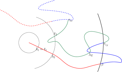
Figure 13: The red curve denotes $\tilde{Y}^{\tau_{i_{N}}}$ and the blue part is $\tilde{X}[\tau_{i_{N}},\tau_{nc}]$.

However, we are still not done as illustrated in Figure 13: the times $t_{1},t_{2}$ (which were first entry, last exit times for $\tilde{\gamma}_{\tilde{v}}$) may be different from $\lambda_{1},\lambda_{2}$ (which were the first entry, last exit of $\tilde{Y}^{\tau_{i_{N}}}$), so we need additional arguments. Let

$$\lambda_{E}:=\inf\{\lambda:\exists t\in[\tau_{i_{N}},\tau_{nc}],\tilde{Y}^{\tau_{i_{N}}}(\lambda)=\tilde{X}(t)\}$$

be the last time in $\tilde{Y}^{\tau_{i_{N}}}$ which is not erased. Note that with this notation we showed above that $\lambda_{E}\geq\beta$. This implies immediately that $t_{1}=\lambda_{1}$. Now we need to consider several cases depending on where $\lambda_{E}$ is in relation to $\lambda_{2}$.

• If $\lambda_{E}\in[\lambda_{1},\lambda_{2}]$, then $\tilde{\gamma}_{\tilde{v}}[t_{1},t_{2}]$ can be decomposed as the union of a piece of $\tilde{Y}^{\tau_{i_{N}}}[\lambda_{1},\lambda_{2}]$ and some erasure of $X[\tau_{i_{N}},\tau_{nc}]$, so on that event

  $$\max_{t_{1}<s_{1}<s_{2}<t_{2}}|W(\tilde{\gamma}_{\tilde{v}}(s_{1},s_{2}),\tilde{v})|\leq\max_{\lambda_{1}<s_{1}<s_{2}<\lambda_{2}}|W(\tilde{Y}^{\tau_{i_{N}}}(s_{1},s_{2}),\tilde{v})|+\Delta$$

  where $\Delta$ is a variable with stretched exponential tail using (6.4).

• If $\lambda_{E}\geq\lambda_{2}$ and $\tilde{\gamma}_{\tilde{v}}(\lambda_{E},t_{2}]$ (the loop erasure after $\lambda_{E}$) does not enter $B(\tilde{v},e^{-t})$ then $\tilde{\gamma}_{\tilde{v}}[t_{1},t_{2}]=\tilde{Y}^{\tau_{i_{N}}}[\lambda_{1},\lambda_{2}]$ and there is nothing more to prove.

• If $\lambda_{E}\geq\lambda_{2}$ and $\tilde{\gamma}_{\tilde{v}}(\lambda_{E},t_{2}]$ enters $B(\tilde{v},e^{-t})$ (this is the case pictured in Figure 13), then we decompose $\tilde{\gamma}_{\tilde{v}}$ as the union of $\tilde{Y}^{\tau_{i_{N}}}[\lambda_{1},\lambda_{2}]$, $\tilde{Y}^{\tau_{i_{N}}}[\lambda_{2},\lambda_{E}]$ and $\tilde{\gamma}_{\tilde{v}}[\lambda_{E},t_{2}]$. The winding of any continuous portion of the first part has exponential tail by (6.3). The winding of any continuous portion of the last part has stretched exponential tail since it is bounded by $\Delta$ as in the first case. So we only need to take care of the middle part.

  To that end, we decompose $\tilde{Y}^{\tau_{i_{N}}}[\lambda_{2},\lambda_{E}]$ into excursions inside and outside $B_{0}$ as follows:

  $$\tilde{Y}^{\tau_{i_{N}}}[\lambda_{2},\lambda_{E}]=\tilde{Y}^{\tau_{i_{N}}}[\lambda_{2},\beta_{0}]\cup\tilde{Y}^{\tau_{i_{N}}}[\beta_{0},\beta_{1}]\cup\tilde{Y}^{\tau_{i_{N}}}[\beta_{1},\beta_{2}]\cup\ldots\cup\tilde{Y}^{\tau_{i_{N}}}[\beta_{k_{0}},\lambda_{E}].$$ (6.5)

  where $\beta_{0}=\beta$ and for $k\geq 1$, $\beta_{2k}$ is the first exit of $B(\tilde{v},e^{-t_{0}})$ after $\beta_{2k-1}$ and $\beta_{2k-1}$ is the first entry into $B(\tilde{v},e^{-t_{0}-1})$ after $\beta_{2k-2}$. Note that any portion of $\tilde{Y}^{\tau_{i_{N}}}[\beta_{2k},\beta_{2k+1}]$ is outside $B(\tilde{v},e^{-t_{0}-1})$ so its winding has exponential tail using Lemma 6.4. Note also that $\tilde{Y}^{\tau_{i_{N}}}[\beta_{2k+1},\beta_{2k+2}]$ lies inside the annulus bounded between $C_{t}$ and $C_{0}$ and never intersects the curve $\tilde{X}[\tau_{i_{N}},\tau_{nc}]$ by maximality of $\lambda_{E}$. Let $Y^{\prime}$ be the loop erasure of the portion of $\tilde{X}$ from $\tau_{i_{N}}$ until its first hit of $C_{t}$. Hence using Lemma 6.3

  $$\max_{\beta_{2k}<s_{1}<s_{2}<\beta_{2k+1}}|W(\tilde{Y}^{\tau_{i_{N}}}(s_{1},s_{2}),\tilde{v})|\leq\max_{s_{1}<s_{2}}|W(Y^{\prime}[s_{1},s_{2}],\tilde{v})|+4\pi$$

  Note that the right hand side has stretched exponential tail by (6.4). Thus each term in the decomposition (6.5) has stretched exponential tail and clearly the number of terms is bounded by $N$ which itself has exponential tail. Combining these two, we can conclude that the absolute value of winding of any continuous portion of $\tilde{Y}^{\tau_{i_{N}}}[\lambda_{2},\lambda_{E}]$ has stretched exponential tail (with exponent $1/3$), thereby completing the proof of this case.

This concludes the proof of Lemma 6.6. ∎

6.3 From partial path to the full spine.

As shown in Theorem 4.10, the path $\tilde{\gamma}_{\tilde{v}}$ defined above is only a part of what is needed to compute the height function. Recall the notion of spine from Section 4.2 which is just a bi-infinite path in the cover. As observed before, when we follow the outgoing edges in the Temperleyan forest from any given $\tilde{v}$, we always end up in a unique spine (since boundary loops have been added around every hole).

Recall from Theorem 4.10 that we are interested in the winding of the path starting from $\tilde{v}$, and then moving along the spine to infinity or the boundary of the disc. Observe that the initial portion of this path is $\tilde{\gamma}_{\tilde{v}}$ (Figure 12) and then it moves along copies of the noncontractible loop in the component of $\tilde{v}$ in the Temperleyan CRSF. In this section, we will call this path $\mathsf{p}_{\tilde{v}}$ (i.e., $\tilde{\gamma}_{\tilde{v}}$ followed by a semi-infinite piece of the spine). Observe that this notation is in contrast to the notation used in Theorem 4.10, where the path $\mathsf{p}_{\tilde{v}}$ was called $\gamma_{f}$, whereas here we emphasise that $\tilde{\gamma}_{\tilde{v}}$ denotes what is sampled from Wilson’s algorithm given the skeleton. When we apply Wilson’s algorithm to sample $\tilde{\gamma}_{\tilde{v}}$, given the skeleton, we may form a new noncontractible loop, in which case we have discovered a portion of a spine (the unique spine attached to $\tilde{v}$). The winding of this portion is controlled by Lemma 6.6. However, we also need to control the winding of the rest of $\mathsf{p}_{\tilde{v}}$. The purpose of this section is precisely to achieve this (done in Lemma 6.7). We also need to control the winding of the other semi-infinite piece of the spine attached to $\tilde{v}$, which is done in Lemma 6.8. Finally, if we want to control the height gap between $\tilde{u}$ and $\tilde{v}$, we need to control the winding of $\mathsf{p}_{\tilde{u}}$ around $\tilde{v}$ as well, which is done in Lemma 6.9.

Let us parametrise $\mathsf{p}_{\tilde{v}}$ in $[0,\infty)$ in any continuous manner away from $\tilde{v}$. Let $t_{0}$ be as in Section 6.2, i.e., $e^{-t_{0}}=\tilde{r}_{\tilde{v}}$. For $t\geq t_{0}$, let $t_{1}$ be the first exit time of $\mathsf{p}_{\tilde{v}}$ from $B(\tilde{v},e^{-t-1})$ and let $t_{2}$ be the last exit time of the same from $B(\tilde{v},e^{-t})$. Note again that here, it is possible that the unique spine attached to $\tilde{v}$ could be the same as the spine corresponding to a skeleton branch.

Lemma 6.7.

For all $k\geq 1$, there exists a constant $m>0$ so that for all $\delta<\delta_{\bar{B}(\tilde{v},e^{-t_{0}})}$ and for all $t_{0}\leq t<\log(C^{\prime}\delta_{0}/\delta)$,

$$\mathbb{E}(\max_{\mathcal{Y}\subseteq\mathsf{p}_{\tilde{v}}[t_{1},t_{2}]\cap B(\tilde{v},e^{-t-1})^{c}}|W(\mathcal{Y},\tilde{v})|^{k}))\leq m.$$

where the supremum is taken over all continuous segments. Also

$$\mathbb{E}(\max_{\mathcal{Y}\subseteq\mathsf{p}_{\tilde{v}}\cap B(\tilde{v},e^{-t_{0}})^{c}}|W(\mathcal{Y},\tilde{v})|^{k}))\leq m$$

Proof.

In this proof, we write $\mathsf{p}_{\tilde{v}}=\mathsf{p}$ to lighten notation. Let us first consider the case when $\mathsf{p}$ does not contain a portion of the spine corresponding to the skeleton.

We parametrise $\tilde{\gamma}_{\tilde{v}}$ in $[0,1]$ as before and assume that the parametrisation of $\tilde{\gamma}_{\tilde{v}}$ and $\mathsf{p}$ is the same until they start to differ. We drop $\tilde{v}$ and write $\tilde{\gamma}_{\tilde{v}}=\gamma$ throughout the rest of this proof for notational clarity. To differentiate the first and last exit times for these two parametrisations we write $t_{1}(\mathsf{p})$ (resp. $t_{2}(\mathsf{p})$) for the first exit of $B(\tilde{v},e^{-t-1})$ (resp. last exit of $B(\tilde{v},e^{-t})$) of $\mathsf{p}$. We also write $t_{1}=t_{1}(\gamma)$ and $t_{2}=t_{2}(\gamma)$ for clarity.

Note that it is always the case that $t_{1}(\gamma)=t_{1}(\mathsf{p})$ and that $t_{2}(\gamma)\leq t_{2}(\mathsf{p})$. On the event $t_{2}(\mathsf{p})=t_{2}(\gamma)$, the maximum in this lemma is over the same set as the one in Lemma 6.6 so there is nothing to prove. We focus now on the case where $t_{2}(\mathsf{p})>t_{2}(\gamma)$, meaning that a part of the spine comes back close to $x$ on the cover $\tilde{M}^{\prime}$ after the time that a noncontractible loop was created.

We start with the case of the torus. Let us denote by $S$ the spine attached to $\tilde{v}$ (meaning the full bi-infinite path). Since $S$ is a periodic path, it has a well-defined direction $d$ (say represented by a unit vector in $\mathbb{R}^{2}$) and separates the plane in two sets right and left of $S$. Let us assume without loss of generality that the direction $d$ is horizontal and that $\tilde{v}$ is below $S$. Let $\tau$ be a time at which the vertical coordinate of $\gamma$ reaches its maximum (for topological reasons, this has to occur on the spine $S$) and let us define $\gamma^{\prime}$ by appending to $\gamma[0,\tau]$ a vertical segment going up to infinity.

Now it is easy to see that the winding of a straight segment around a point is bounded by $\pi$, so

$$\max_{\mathcal{Y}\subseteq\gamma^{\prime}\cap B(\tilde{v},e^{-t-1})^{c}}|W(\mathcal{Y},\tilde{v})|\leq\max_{\mathcal{Y}\subseteq\gamma\cap B(\tilde{v},e^{-t-1})^{c}}|W(\mathcal{Y},\tilde{v})|+\pi.$$ (6.6)

Using Lemma 6.3, this implies that we can always bound

$$\max_{\mathcal{Y}\subseteq{\mathsf{p}_{\tilde{v}}}\cap B(\tilde{v},e^{-t-1})^{c}}|W(\mathcal{Y},\tilde{v})|\leq\max_{\mathcal{Y}\subseteq\gamma^{\prime}\cap B(\tilde{v},e^{-t-1})^{c}}|W(\mathcal{Y},\tilde{v})|+4\pi\leq\max_{\mathcal{Y}\subseteq\gamma\cap B(\tilde{v},e^{-t-1})^{c}}|W(\mathcal{Y},\tilde{v})|+5\pi.$$ (6.7)

By Lemma 6.6 (the $\tilde{\gamma}_{\tilde{v}}$ there is $\gamma$ here) applied to all scales up to scale $t$, the right hand side is a sum of $O(t)$ variables with uniform stretched exponential tails.

Let us now bound $\mathbb{P}(t_{2}({\mathsf{p}})>t_{2}(\gamma);\mathsf{p}\cap\mathfrak{s}=\emptyset)$. Note that on the event $t_{2}(\mathsf{p})>t_{2}(\gamma)$, $\tilde{v}$ has to be at distance less that $e^{-t}$ of its spine. Using the fact that we can sample points in any order in Wilson’s algorithm, we can bound that probability by first doing a cutset exploration around $\tilde{v}$ at scale $r_{\tilde{v}}$. After this cutset exploration, the probability that any of the branches sampled intersects $B(\tilde{v},e^{-t})$ is at most $Ce^{-c(t-t_{0})}$ for some constants $C,c$ (see Lemma 5.6). At the same time, after the cutset exploration around $\tilde{v}$ the spine attached to $\tilde{v}$ is necessarily fully sampled (see e.g., Proposition 5.9, final assertion). Hence

$$\mathbb{P}(t_{2}({\mathsf{p}})>t_{2}(\gamma);\mathsf{p}\cap\mathfrak{s}=\emptyset)\leq Ce^{-c(t-t_{0})}.$$ (6.8)

Thus overall, either $\max_{\mathcal{Y}\subseteq{\mathsf{p}[t_{1},t_{2}]}\cap B(\tilde{v},e^{-t-1})^{c}}|W(\mathcal{Y},\tilde{v})|$ is the same as the variable in Lemma 6.6, or with probability at most $Ce^{-c(t-t_{0})}$, it is at most a sum of $O(t)$ variables with uniform stretched exponential tail. The moment bound now easily follows.

For the case where the universal cover is the unit disc, a similar argument can be done provided we can construct a path $\gamma^{\prime}$ which is nice and avoids the spine. Let us also introduce $\tau_{S}$ as the first time $\gamma$ hits the spine and $\tau_{nc}$ as the ending time of $\gamma$. As recalled in more details in appendix A, it is a well known fact from Riemann surfaces that there exists a Möbius transform $\phi=\phi_{\gamma,\tilde{v}}$ such that

$${\mathsf{p}}(v)=\gamma[0,\tau_{S}]\cup\bigcup_{n\geq 0}\phi^{(n)}((\tau_{S},\tau_{nc}])$$

where $\phi^{(n)}=\phi\circ\ldots\circ\phi$ and the union is disjoint. In other words, we keep applying the same Möbius transform to obtain all the copies. Furthermore $\phi$ can be written as $\phi=\Phi^{-1}\circ\mu\circ\Phi$ where $\Phi$ is a Möbius map from the unit disc to the upper half plane and $\mu$ is either the translation by $\pm 1$ or a multiplication by $\lambda>1$.

If it is a translation we use the same argument as before. Otherwise, it is a scaling by $\lambda>1$ in which case $\phi(S)$ necessarily converges to infinity. Furthermore, let $\tau$ be the time at which $\Im(\Phi(\gamma))$ reaches its minimum, we define $\gamma^{\prime}$ by appending a straight vertical segment $\ell$ from $\Phi(\gamma(\tau))$ to $\mathbb{R}$ (note that this segment may not intersect $\Phi(\gamma)$ nor the subsequent scalings of the image of the portion of the spine $\Phi(\gamma([\tau_{S},\tau_{nc}])$) and then mapping $\Phi(\gamma[0,\tau]\cup\ell)$ back to the disc by $\Phi^{-1}$. By construction, it is trivial to check that $\Phi(\gamma^{\prime})$ does not intersects $\Phi({\mathsf{p}}(\tau,\infty))$ so $\gamma^{\prime}$ does not intersect ${\mathsf{p}}(\tau,\infty)$. On the other hand, $\Phi^{-1}$ is the image of a line segment by a Möbius transform so it is a circular arc and therefore its winding around any point is bounded by $2\pi$. We can then conclude using exactly the same reasoning as in the torus case, with only the constant $\pi$ replaced by $2\pi$ on the right hand side of (6.6) and hence obtain the analogue of (6.7).

Finally, let us consider the case when $\mathsf{p}$ contains a portion of the spine corresponding to the skeleton. Note that the whole argument was geometric and the only place where we used the probability was in (6.8) which is provided by Lemma 5.5. ∎

Lemma 6.8.

For all $k\geq 1$, there exist a constant $C>0$ such that the following holds. Fix a compact set $K\subset\tilde{M}^{\prime}$ . Suppose we are in the setup of Lemma 6.7. Let $\mathsf{p}=\mathsf{p}_{\tilde{v}}$ be as above and $\bar{\mathsf{p}}$ be the curve which starts at $\tilde{v}$, hits the spine, and then goes to infinity in the direction opposite to the orientation of the spine. Orient and parametrise both $\mathsf{p},\bar{\mathsf{p}}$ from $\tilde{v}$ to $\infty$ so that $t_{2}$ is the last time they exit $B(\tilde{v},e^{-t})$. Then for all $\delta<\delta_{K},t\in[t_{0},\infty],\tilde{v}\in K$,

$$\mathbb{E}\Big{(}\sup_{\mathcal{Y}\subset\mathsf{p}[t_{2},\infty)}|W(\mathcal{Y},\tilde{v})|^{k}\Big{)} \leq C((1+t)\wedge\log(1/\delta))^{k},$$

$$\mathbb{E}\Big{(}\sup_{\mathcal{Y}\subset\mathsf{\bar{p}}[t_{2},\infty)}|W(\mathcal{Y},\tilde{v})|^{k}\Big{)} \leq C((1+t)\wedge\log(1/\delta))^{k}.$$

We emphasize here that the spine might be identical to a spine of a skeleton branch.

Proof.

First we tackle the case of $\mathsf{p}$. If $t<\log(C^{\prime}\delta_{0}/\delta)$, we need to add $O(t)$ many variables given by Lemma 6.7 and hence we are done by Minkowski’s inequality. If $t>\log(C^{\prime}\delta_{0}/\delta)$, first we apply the previous bound up to $t=\log(C^{\prime}\delta_{0}/\delta)$. For the remainder, we can simply bound the winding by the volume of the ball of radius $C^{\prime}\delta/\delta_{0}$ around $\tilde{v}$ which is $O(1)$ by our assumptions on the graph (see assumption (i) in Section 2.3). Indeed, this quantity is bounded by the number of times $\mathsf{p}$ crosses a straight line joining $\tilde{v}$ to the boundary of the ball, which is simply bounded by the volume of the ball. For $\mathsf{\bar{p}}$, we can use Lemma 6.3 and the bound for $\mathsf{p}$ and the proof is complete. ∎

Lemma 6.9.

For all $k$ there exist $C,c>0$ such that for all points $\tilde{u},\tilde{v}$, for all compact sets $\tilde{K}$ containing $\tilde{u},\tilde{v}\in\tilde{M}^{\prime}$ , for all $\delta<\delta_{\tilde{K}}$,

$$\mathbb{E}\Big{(}|W(\mathsf{p}_{\tilde{u}},\tilde{v})|^{k}\Big{)}\leq C(|1+\log|\tilde{u}-\tilde{v}||\wedge\log(1/\delta))^{c}.$$

Proof.

Fix $T=\log(\frac{C^{\prime}\delta_{0}}{\delta})$ with $C^{\prime}$ as in Lemma 6.7. We parametrise $\mathsf{p}_{\tilde{v}},\mathsf{p}_{\tilde{u}}$ as in Lemma 6.8. If $|\tilde{u}-\tilde{v}|<e^{-T}$, we use Lemmas 6.8 and 6.3 to conclude.

If $|\tilde{u}-\tilde{v}|\geq e^{-T}$, we take $t=-\log|\tilde{u}-\tilde{v}|$. Then using Lemma 6.3, we can write

$$|W(\mathsf{p}_{\tilde{u}},\tilde{v})|\leq 2\pi+\sum_{k=t}^{\infty}\sup_{\mathcal{Y}\subset\mathsf{p}_{\tilde{v}}[k_{2},\infty)}|W(\mathcal{Y},\tilde{v})|1_{|\mathsf{p}_{\tilde{u}}-\tilde{v}|\in[e^{-k},e^{-k-1}]}$$

where $k_{2}$ is the last exit from the $B(\tilde{v},e^{-k})$ by $\mathsf{p}_{\tilde{u}}$. Using Lemma 5.3 or Lemma 5.5 whichever is appropriate, we get an exponential bound on the expectation of the indicator event above (notice for scales $k>\log(C^{\prime}\delta_{0}/\delta)$, the probability actually becomes 0 so this is a finite sum). Therefore, we can again use Lemma 6.8 and Cauchy–Schwarz to conclude. ∎

6.4 Convergence of height function

In this section we prove Theorem 6.1.

Let us describe informally the general structure of the proof. Most of the work will be in the universal cover to obtain the convergence of expressions of the form $\mathbb{E}\prod_{i}(h(\tilde{z}_{i})-h(\tilde{w}_{i}))$ for distinct points $\tilde{z}_{i}$ and $\tilde{w}_{i}$ (Lemma 6.11). By integrating this expression, we will then obtain the convergence of the height function, seen as a function on the universal cover.

As mentioned in the introduction, for the first part, the idea is to introduce a regularised height function $h^{\#\delta}_{t}$ which is a continuous function of the CRSF so that the convergence of $h^{\#\delta}_{t}$ as $\delta\rightarrow 0$ is immediate. This leaves us with two issues: the comparison between $h^{\#\delta}$ and $h^{\#\delta}_{t}$ for fixed $\delta$ and the convergence of $h_{t}$ as $t\rightarrow\infty$ in the limit. Both questions are actually solved simultaneously by the estimate of Lemma 6.11 which compares $h^{\#\delta}$ and $h^{\#\delta}_{t}$ with an error term that becomes small both in $\delta$ and $t$ independently.

Setup and notations.

Recall that our goal is to prove that

$$\int_{\tilde{M}^{\prime}}\overline{h}_{\textsf{ext}}^{\#\delta}(z)\tilde{f}(z)d\mu(z)$$ (6.9)

converges in law and also in the sense of moments as $\delta\to 0$. (Recall that $\bar{X}$ denote the centered random variable $\bar{X}=X-\mathbb{E}(X)$ whenever this expectation is well defined). Implicitly, $h^{\#\delta}$ is sampled according to the dimer law (1.1). In other words, by Theorem 3.3, we need to first sample a Temperleyan pair $(\mathcal{T},\mathcal{T}^{\dagger})$ and apply the bijection $\psi$ in that theorem.

However, it turns out to be more convenient in the proof to work with a pair $(\mathcal{T},\mathcal{T}^{\dagger})$ sampled from $\operatorname{\mathbb{P}_{Wils}}$. To this pair $(\mathcal{T},\mathcal{T}^{\dagger})$ we can apply the bijection $\psi$ from Theorem 3.3 and obtain a dimer configuration $\mathbf{m}$ whose centered height function can be studied. We will first prove (6.9) for $\operatorname{\mathbb{P}_{Wils}}$ and then later explain how this implies the same for $\operatorname{\mathbb{P}_{Temp}}$.

Recall that since $\int_{\tilde{M}^{\prime}}\tilde{f}(z)d\mu(z)=0$, the expression in (6.9) is in fact well-defined. We wish to compute the moments of this integral but only in terms of height differences since the field is a priori defined only up to constant. To do this, we use the following trick. Note that since $\int\tilde{f}d\mu=0$, $\int\tilde{f}^{+}d\mu=\int\tilde{f}^{-}d\mu=:Z(\tilde{f})$ where $f^{+}=\max\{f,0\}$ and $f^{-}=-\min\{f,0\}$. Now we can write

$$\int_{\tilde{K}}\overline{h}_{\textsf{ext}}^{\#\delta}(z)\tilde{f}(z)d\mu(z)=\int_{\tilde{K}\times\tilde{K}}(\overline{h}_{\textsf{ext}}^{\#\delta}(z)-\overline{h}_{\textsf{ext}}^{\#\delta}(w))\frac{\tilde{f}^{+}(z)\tilde{f}^{-}(w)}{Z(\tilde{f})}d\mu(z)d\mu(w).$$ (6.10)

which implies

$$(\int_{\tilde{K}}\overline{h}_{\textsf{ext}}^{\#\delta}(z)\tilde{f}(z)d\mu(z))^{k}=\int_{\tilde{K}^{2k}}\prod_{i=1}^{k}(\overline{h}_{\textsf{ext}}^{\#\delta}(z_{i})-\overline{h}_{\textsf{ext}}^{\#\delta}(w_{i}))\frac{\tilde{f}^{+}(z_{i})\tilde{f}^{-}(w_{i})}{Z(\tilde{f})}d\mu(z_{i})d\mu(w_{i})$$ (6.11)

Therefore we are interested in the $k$-point function, $\mathbb{E}[\prod_{i=1}^{k}(\overline{h}_{\textsf{ext}}^{\#\delta}(z_{i})-\overline{h}_{\textsf{ext}}^{\#\delta}(w_{i}))]$. Pick $k$ distinct pairs of points $(z_{1},w_{1}),\ldots,(z_{k},w_{k})\in\tilde{K}$ and let $(f(z_{1}),f(w_{1})),\ldots,(f(z_{k}),f(w_{k}))$ be the faces containing them. Let $z_{i}^{\#\delta},w^{\#\delta}_{i}$ be the midpoint of the diagonals of $f(z_{i}),f(w_{i})$.

Now recall Theorem 4.10 which relates the dimer height difference between two faces $f$ and $f^{\prime}$ to the winding of a specific path $\gamma_{f,f^{\prime}}$ connecting $m(f)$ and $m(f^{\prime})$ and additional terms of the form $\pm\pi$ associated with jumping over components of the CRSF. Let $\gamma_{i}^{\#\delta}$ be the path $\gamma_{f,f^{\prime}}$ when $f=f(z_{i})$ and $f^{\prime}=f(w_{i})$, and orient it from $z_{i}^{\#\delta}$ to $w_{i}^{\#\delta}$. Then with these notations, Theorem 4.10 says that

$$h(z_{i}^{\#\delta})-h(w_{i}^{\#\delta})=W(\gamma_{i}^{\#\delta},z_{i}^{\#\delta})+W(\gamma_{i}^{\#\delta},w_{i}^{\#\delta})+\Psi^{\#\delta}_{i}$$ (6.12)

where $\Psi^{\#\delta}_{i}$ is the $\pi\sum_{S}(\varepsilon_{S}+\delta_{S})$ term in Theorem 4.10. We drop the superscript $\delta$ from now on for clarity. Thus from now on we focus on proving convergence of

$$\operatorname{\mathbb{E}_{Wils}}\Big{(}\prod_{i=1}^{k}(\bar{W}(\gamma_{i},z_{i})+\bar{W}(\gamma_{i},w_{i})+\bar{\Psi}_{i})\Big{)}$$ (6.13)

Let

$$\mathcal{X}=\{z_{i},w_{i}:1\leq i\leq k\},\text{ and assume }p(u)\neq p(v)\text{ for all }u\neq v\in\mathcal{X}.$$

Clearly, (6.13) can be expanded as a sum of $2^{k}$ many terms of the form:

$$\operatorname{\mathbb{E}_{Wils}}(\prod_{x\in S}(\bar{W}(\gamma_{x},x)+\bar{\Psi}_{x}/2))=:\operatorname{\mathbb{E}_{Wils}}(\prod_{x\in S}\bar{F}_{x}(\gamma_{x}))$$ (6.14)

where $S$ is a subset of vertices of $\mathcal{X}$ with distinct indices and $\gamma_{x}$ is $\gamma_{i}$ for some $i$ such that $x=z_{i}$ or $w_{i}$ (of course, the products in the expansion of (6.14) has further restrictions, but we ignore that for clarity).

We are interested in estimating and proving convergence of (6.14). To that end we employ an idea similar to that in [4]: we truncate the CRSF branch at a macroscopic scale and deal with the truncated macroscopic winding and the remaining microscopic winding part separately.

We now fill in the details. Parametrise $\gamma=\gamma_{x}$. Define $(\gamma_{x}(t))_{t\geq 1}$ to be $\gamma_{x}$ at the first entry time into the ball $B(x,e^{-t})$ (Note that at the moment, $B(x,e^{-t})$ might overlap for different $x\in\mathcal{X}$.) We emphasise here that we parametrise $\gamma$ in the opposite direction compared to Sections 6.2 and 6.3 to be consistent with [4]. With an abuse of notation, we will denote by $\gamma_{x}(-\infty,t]$ the whole path from the opposite end of $\gamma$ up until $\gamma_{x}(t)$. Define the regularised term and the error term as

$$\bar{F}_{x}(\gamma_{x},t) :=\bar{W}(\gamma_{x}(-\infty,t]);x)+\bar{\Psi}_{x}/2$$ (6.15)

$$\bar{e}_{x}(t) :=\bar{W}(\gamma_{x},x)-\bar{W}(\gamma_{x}(-\infty,t]),x)=\bar{F}_{x}(\gamma_{x})-\bar{F}_{x}(\gamma_{x},t).$$ (6.16)

When we want to emphasise the role of $z,w$, we write $\gamma_{zw},\Psi_{zw},F_{z}(\gamma_{zw})$ in place of the above. We start with a general moment bound for the truncated winding.

Lemma 6.10.

For all $m$, there exists constants $c=c(\tilde{K},m),\alpha=\alpha(m)$ such that for all $z,w,\delta<\delta_{\tilde{K}},t\geq 0$,

$$\operatorname{\mathbb{E}_{Wils}}(|\bar{F}_{z}(\gamma_{zw},t)|^{m})\leq c|(1+t+|\log|z-w||)\wedge\log(1/\delta)|^{\alpha}$$

Proof.

The proof is immediate from Lemmas 6.8 and 6.9 and the fact that $\Psi_{zw}$ is bounded by a constant $c(K)$ times the number of noncontractible loops in the CRSF. Indeed, this is clear from the fact that for a fixed compact set $\tilde{K}\subset\tilde{M}$ there exists a constant $c(\tilde{K})$ such that any curve $P\subset\tilde{K}$ will cross at most $c(\tilde{K})$ copies of a given spine (or lift of a loop). Since the number of noncontractible loops has superexponential tail ([5, Theorem 3.1]), the moment bound of $\Psi_{zw}$ is immediate. ∎

By compactness, choose $r_{\tilde{K}}$ small enough so that $p$ is injective in $B(z,r_{\tilde{K}})$ for all $z\in\tilde{K}$. Now let $r_{\mathcal{X}}$ be defined as in (5.1) but for the set of vertices $p(\mathcal{X})$ (which are all distinct by assumption on $\mathcal{X}$). We observe that $r_{\mathcal{X}}\geq c(\tilde{K})\min_{x\neq y\in\mathcal{X}}|x-y|$ for some constant $c(\tilde{K})$. We set

$$\Delta=\Delta(\mathcal{X})=\frac{1}{10}(r_{\mathcal{X}}\wedge r_{\tilde{K}})$$ (6.17)

Lemma 6.11.

There exist constants $c,c^{\prime}>0$ such that for all $m,m^{\prime}\geq 1$ there exists $\alpha>0$ such that the following holds. Let $S\subset\mathcal{X},S^{\prime}\subset\mathcal{X}$ be disjoint. Also assume that $|S|=m,|S^{\prime}|=m^{\prime}\geq 0$. Let $\Delta$ be as in (6.17). Then for all $\delta<\delta_{\tilde{K}}$ and $t\geq\log(r_{\tilde{K}}/\Delta)$

$$|\operatorname{\mathbb{E}_{Wils}}(\prod_{x\in S}\bar{e}_{x}(t)\prod_{x\in S^{\prime}}\bar{F}_{x}(t))|\leq c|1+t|^{\alpha}(e^{-c(t-\log(r_{\tilde{K}}/\Delta))}+\delta^{c^{\prime}}).$$

Proof.

For simplicity, we first assume $S^{\prime}$ is empty. Recall that we can sample a CRSF from $\operatorname{\mathbb{P}_{Wils}}$ by first sampling the branches $\mathfrak{s}$ and then the rest by Wilson’s algorithm. Note that Lemma 5.5 tells us that the isolation radius corresponding of each vertex in $S$ with respect to the skeleton has polynomial tail. Since after sampling the skeleton, the rest of the branches are sampled simply by Wilson’s algorithm, we can conclude that the application of Proposition 5.9 is valid with $\Delta$ in place of $r_{i}$.

We perform the coupling in Section 5.2 (in particular Proposition 5.9) with points $p(\mathcal{X})$ and their lift $\mathcal{X}$, and a compact domain $D\subset\tilde{M}^{\prime}$ containing all points in $\mathcal{X}$ so that the minimal Euclidean distance between any point in $\mathcal{X}$ and $\partial D$ is at least $r_{\mathcal{X}}$. Note that we can choose $r_{\mathcal{X}}$ for the $r$ in (5.1) there. Call $(\mathcal{T}^{D}_{x})_{x\in\mathcal{X}}$ the resulting independent UST in $D$. For $x\in\mathcal{X}$ let $\gamma^{D}_{x}$ be the branch in the UST $\mathcal{T}^{D}_{x}$ joining $x$ to $\partial D$. Let $\gamma_{x}^{D}(t)$ be parametrised so that $\gamma^{D}_{x}$ enters $B(x,e^{-t}r_{\tilde{K}})$ for the first time (going from the outside to $x$) at time $t$.

Let $R_{x}$ be the isolation radius of $x$ in the application of Proposition 5.9 and write $R_{x}=e^{-I_{x}}r_{\tilde{K}}$. Let $I=\max_{x\in\mathcal{X}}I_{x}$. (Note that for notational clarity, $I$ here is shifted by $\log(r_{\tilde{K}}/\Delta)$ from that in Section 5.2.) We now decompose

$$e_{x}(t) =\underbrace{\overline{W}(\gamma^{D}_{x}(t,\infty),x)}_{\alpha_{x}}+\underbrace{(\overline{W}(\gamma_{x}(t,\infty),x)-\overline{W}(\gamma^{D}_{x}(t,\infty),x))}_{\xi_{x}}$$ (6.18)

Therefore, we need to deal with expectation of products of $\alpha_{x},\xi_{x}$ for different indices $x$. Let $\mathfrak{C}$ be the sigma algebra generated by the cutset exploration. We will first compute the conditional expectation and then take the overall expectation. Note that $\mathcal{T}_{x}^{D}$ are independent for different $x$ and also independent of $\mathfrak{C}$ and hence any term involving $\alpha_{x}$ is 0. Thus we only have to deal with terms involving $\xi_{x},x\in S$.

Let $\Lambda$ be the last time $\gamma_{x}$ enters $B(x,e^{-I}r_{\tilde{K}})$. In the coupling, $\gamma_{x},\gamma_{x}^{D}$ agree inside $B(x,e^{-I}r_{\tilde{K}})$ so in particular $\gamma_{x}(\Lambda,\infty)=\gamma_{x}^{D}(\Lambda,\infty)$, so

$$\xi_{x}=\overline{W}(\gamma_{x}(t,\Lambda),x)-\overline{W}(\gamma^{D}_{x}(t,\Lambda),x).$$

Let $G$ be the event that $\xi_{x}$ without the bar (meaning without the expectation terms) is 0. Observe that if $G$ does not occur then one of the following events happen. Either

$$I-\log(r_{\tilde{K}}/\Delta)>(t-\log(r_{\tilde{K}}/\Delta))/2$$

which has probability at most $e^{-c(t-\log(r_{\tilde{K}}/\Delta))}\vee\delta^{c}\leq(e^{-c(t-\log(r_{\tilde{K}}/\Delta))}+\delta^{c})$ (Proposition 5.9). Otherwise, $\gamma_{x}$ has to exit $B(x,e^{-I}r_{\tilde{K}})$ after hitting $e^{-t}r_{\tilde{K}}$. This also has probability at most $e^{-c(t-\log(r_{\tilde{K}}/\Delta))}$ (Lemma 5.7). Now we bound the moments of $\xi_{x}$. Notice that we can write

$$\operatorname{\mathbb{E}_{Wils}}(|\xi_{x}|^{k}) \leq\sum_{j=t/2+\log(r_{\tilde{K}}/\Delta)/2}^{\infty}\mathbb{E}(|\xi_{x}|^{k}1_{j\leq I\leq j+1})+ce^{-c(t-\log(r_{\tilde{K}}/\Delta))}$$

$$\leq\sum_{j=t/2+\log(r_{\tilde{K}}/\Delta)/2}^{\infty}|1+j|^{k}(e^{-c(j-\log(r_{\tilde{K}}/\Delta))}+\delta^{c})$$

where we first used Cauchy–Schwarz and then used Lemma 6.8 to bound the moment and Proposition 5.9. Thus overall

$$\operatorname{\mathbb{E}_{Wils}}(|\xi_{x}|^{k})\leq|1+t|^{k}(e^{-c(t-\log(r_{\tilde{K}}/\Delta))}+\delta^{c}).$$

We have a product of at most $m$ terms and so using Hölder’s inequality, taking $\alpha=m$ works.

Finally, if $S^{\prime}$ is non-empty, the proof is exactly the same as the vertices in $S^{\prime}$ are distinct from $S$ and hence local independence from the coupling still holds. We then use Lemma 6.10 to conclude using Cauchy–Schwarz. Details are left to the reader. ∎

Corollary 6.12.

Let $S\subset\mathcal{X}$ containing vertices with distinct indices such that $|S|=m$. There exists a constant $c=c(\tilde{K},m),\alpha=\alpha(m)$ such that for all $\delta<\delta_{\tilde{K}}$,

$$|\operatorname{\mathbb{E}_{Wils}}(\prod_{x\in S}\bar{F}_{x}(\gamma_{x}))|\leq c|1+\log^{\alpha}(\Delta)|$$

Proof.

Decompose

$$\operatorname{\mathbb{E}_{Wils}}(\prod_{x\in S}\bar{F}_{x}(\gamma_{x}))=\operatorname{\mathbb{E}_{Wils}}(\prod_{x\in S}(\bar{F}_{x}(\gamma_{x},t)+\bar{e}_{x}(t)))$$ (6.19)

with $t=2\log(r_{\tilde{K}}/\Delta)$. Then this is a straightforward application of Lemmas 6.11 and 6.10. ∎

Now we prove a convergence of the height function integrated against $f$ in the sense of moments (still for the Wilson law $\operatorname{\mathbb{P}_{Wils}}$). Recall that $X_{\delta}$ converges in the sense of moments as $\delta\to 0$ if for all $k$, $\mathbb{E}(X_{\delta}^{k})$ converges as $\delta\to 0$.

Lemma 6.13.

$\int_{\tilde{K}}\overline{h}_{\textsf{ext}}^{\#\delta}(z)\tilde{f}(z)d\mu(z)$ converges in the sense of moments under the law $\operatorname{\mathbb{P}_{Wils}}$. Furthermore, the limit does not depend on the sequence $(G^{\prime})^{\#\delta}$.

Proof.

Using eqs. 6.11, 6.13 and 6.14, we need to prove the convergence as $\delta\to 0$ of

$$\int_{\tilde{K}^{2k}}\operatorname{\mathbb{E}_{Wils}}(\prod_{x\in S}\bar{F}_{x}(\gamma^{\#\delta}_{x}))\frac{\tilde{f}^{+}(z_{i})\tilde{f}^{-}(w_{i})}{Z(\tilde{f})}d\mu(z_{i})d\mu(w_{i})$$ (6.20)

We use Fubini to bring the expectation inside the integral in the above display. We first observe that integrating (6.20) over all sets of vertices $S$ so that $p(x)\neq p(y)$ for all $x\neq y\in S$ is enough (recall $p:\tilde{M}^{\prime}\mapsto M^{\prime}$ is the covering map). Indeed, using Lemma 6.10 and the fact that $\|f\|_{\infty}<\infty$, we see that the integrand can be bounded by $O(\log^{\alpha}(1/\delta))$. Since the volume of $\{S\subset\tilde{K}^{2k}:p(x)=p(y)\text{ for some }x,y\in S\}$ is $O(\delta)$ (indeed the number of preimages of any vertex in $\tilde{K}$ is bounded by a constant depending only on $\tilde{K}$), we see that the integral over this set is $O(\delta\log^{\alpha}(1/\delta))$.

Thus we now concentrate on the integral (6.20) over

$$\mathcal{A}(\tilde{K})=\{\text{sets of vertices }S\text{ so that }p(x)\neq p(y)\text{ for all }x\neq y\in S\}$$ (6.21)

We now use Corollary 6.12 and dominated convergence theorem. Since $\|f\|_{\infty}<\infty$ and $\log^{m}(\Delta)$ is integrable for any $m>0$, we need to prove convergence of the expectation inside the integral above. Now we claim that the regularised part

$$\operatorname{\mathbb{E}_{Wils}}(\prod_{x\in S}\bar{F}_{x}(\gamma^{\#\delta}_{x},t))$$ (6.22)

converges as $\delta\to 0$. This follows from our assumption of a.s. convergence of Temperleyan CRSF and because the term inside the expectation is a.s. continuous function of the Temperleyan CRSF. The same can be said about the skeleton using the absolute continuity statement given by [5, Proposition 6.5] (see also (5.3)). Indeed, this follows from a.s. continuity properties of SLE₂ and the fact that the CRSF branches are made a.s. from finitely many chunks of SLE₂, in particular for a fixed $t$, the SLE curve is a.s. not a tangent to the boundary of circle of radius $e^{-t}$ (we refer to [5, Section 3]) for details. Lemma 6.10 tells us that the random variable in (6.22) is uniformly integrable which completes the proof of convergence of the regularised term (6.22).

Now given a fixed $S$, choose $t\geq\log(r_{\tilde{K}}/\Delta)$. Now we claim that that the error term satisfies

$$|\operatorname{\mathbb{E}_{Wils}}(\prod_{x\in S}\bar{F}_{x}(\gamma_{x}))-\operatorname{\mathbb{E}_{Wils}}(\prod_{x\in S}\bar{F}_{x}(\gamma_{x},t))|<c|1+t|^{\alpha}(e^{-c(t-\log(r_{\tilde{K}}/\Delta))}+\delta^{c^{\prime}})$$ (6.23)

Indeed, (6.23) follows by writing $\bar{F}_{x}(\gamma_{x})=\bar{F}_{x}(\gamma_{x},t)+\bar{e}_{x}(t)$ and then expanding and using the bounds in Lemmas 6.10 and 6.11. To finish the proof of the lemma, fix $\varepsilon>0$. First choose $t$ large enough and then $\delta$ small enough so that the right hand side of (6.23) is less than $\varepsilon$. Next choose a smaller $\delta$ if needed so that for all $\delta^{\prime}<\delta$,

$$|\operatorname{\mathbb{E}_{Wils}}(\prod_{x}\bar{F}(\gamma^{{\#\delta}^{\prime}}_{x},t))-\operatorname{\mathbb{E}_{Wils}}(\prod_{x}\bar{F}_{x}(\gamma^{{\#\delta}}_{x},t))|<\varepsilon.$$

via the convergence of the regularised term. This completes the proof as $\varepsilon$ is arbitrary.

Observe that (6.23) completes the proof that the limit does not depend on the sequence $((G^{\prime})^{\#\delta})_{\delta>0}$ since the main term (6.22) is measurable with respect to the limiting continuum Temperleyan CRSF which is universal by [5, Theorem 1.1]. ∎

It remains to prove convergence in law (still for $\operatorname{\mathbb{P}_{Wils}}$ for now). For this, we need to alter the definition of truncation slightly. Given $t>0$, take a cover $\{B_{\textsf{euc}}(x,r_{\tilde{K}}e^{-10t}):x\in\tilde{K}\}$ of $\tilde{K}$ and take a finite subcover. Let $\mathfrak{c}(z),\mathfrak{c}(w)$ denote the center of one of the balls (chosen arbitrarily) in the finite subcover in which $z,w$ belong. Define $\mathsf{F}_{x}(t),\mathsf{e}_{x}(t)$ to be the same as $F_{x}(t)$ and $e_{x}(t)$ but we cut off the first time $\gamma_{x}$ enters $B(\mathfrak{c}(x),e^{-t})$ (so compared to the above, the centre of the cutoff ball is shifted by an amount which is at most $e^{-10t}$). However, in this definition, we still measure winding around $x$ not $\mathfrak{c}(x)$.

Lemma 6.14.

The statements of Lemmas 6.10 and 6.11 still hold if we replace $F,e$ by $\mathsf{F},\mathsf{e}$ everywhere.

Proof.

For Lemma 6.10, the proof identically follows from Lemmas 6.8 and 6.9 by noticing that the supremum over all continuous subpaths contain the portion of the branch until it first hits the shifted ball. Notice also that we shift only by an additive term in the exponential scale which is $O(t)$.

For Lemma 6.11, the proof is also identical, in particular we still consider the coupling around the points in $S$. Because we still shift only by $O(t)$ in the exponential scale, the proof readily follows. ∎

We can now complete the proof of Theorem 6.1.

Proof of Theorem 6.1.

Again, we first prove this under $\operatorname{\mathbb{P}_{Wils}}$ before explaining how to extend this and concluding the proof of Theorem 6.1 to $\operatorname{\mathbb{P}_{Temp}}$. We write $r=r_{\tilde{K}}$ and pick a $t>0$ to be taken large later. Recall from eqs. 6.10 and 6.12,

$$\int_{\tilde{K}}\overline{h}_{\textsf{ext}}^{\#\delta}(z)\tilde{f}(z)d\mu(z)=\int_{\tilde{K}\times\tilde{K}}(\bar{W}(\tilde{\gamma}^{\#\delta}_{zw},z)+\bar{W}(\tilde{\gamma}_{zw}^{\#\delta},w)+\bar{\Psi}_{zw})\frac{\tilde{f}^{+}(z)\tilde{f}^{-}(w)}{Z(\tilde{f})}d\mu(z)d\mu(w).$$

Here $Z(\tilde{f})$ is a deterministic constant so we can assume it to be 1 from now on without loss of generality. Firstly we recall that we only need to integrate over the set $\mathcal{A}(\tilde{K})$ as in (6.21) as the integral over the remaining part is $O(\delta\log^{c}(1/\delta))$. Let us denote by $Y=Y(\delta)$ the above integral over $\mathcal{A}(\tilde{K})$. Introduce

$$X(\delta,t):=\int_{\mathcal{A}(\tilde{K})}(\bar{\mathsf{F}}_{\mathfrak{c}(z)\mathfrak{c}(w)}(t)+\bar{\mathsf{F}}_{\mathfrak{c}(w)\mathfrak{c}(z)}(t))1_{|\mathfrak{c}(z)-\mathfrak{c}(w)|>re^{-t/10}}\tilde{f}^{+}(z)\tilde{f}^{-}(w)d\mu(z)d\mu(w)$$

Note that $X(\delta,t)$ is a sum of regularised winding of finitely many branches and hence converges in law (as $\delta\to 0$ and $t$ is fixed) by our assumption.

Now we show that for all $t>0$ and $\delta<C^{\prime}\delta_{0}e^{-t}$,

$$\mathbb{E}(Y(\delta)-X(\delta,t))^{2}\leq c(1+t)^{\alpha}e^{-c^{\prime}t}.$$

We expand the above square to get an integral over $(z,w,z^{\prime},w^{\prime})\in\mathcal{A}(\tilde{K})^{2}$. We can again without loss of generality restrict to the the set $\mathcal{A}_{2}(\tilde{K})$ such that the projection $p$ of all four points $(z,w,z^{\prime},w^{\prime})$ maps to pairwise distinct points on $M$. In that case let $\Delta=\Delta(z,w,z^{\prime},w^{\prime})$ be as in (6.17). We now argue that this integral over the set $\Delta\leq e^{-t/11}$ is exponentially small in $t$. Indeed, we are integrating over a set which has exponentially small measure with respect to $\mu^{4}$ and furthermore the moments are integrable using Corollaries 6.12 and 6.14.

For the rest of the integral, we write

$$(\bar{W}(\tilde{\gamma}^{\#\delta}_{zw},z)+\bar{W}(\tilde{\gamma}_{zw}^{\#\delta},w)+\bar{\Psi}_{zw})=\bar{\mathsf{F}}_{zw}(t)+\bar{\mathsf{F}}_{wz}(t)+\bar{\mathsf{e}}_{zw}(t)+\bar{\mathsf{e}}_{wz}(t)$$

and we expand again the product inside the integral to get products of terms of the form

$$\bar{\mathsf{e}}_{zw}(t)+\bar{\mathsf{e}}_{wz}(t);\quad\bar{\mathsf{F}}_{zw}(t)+\bar{\mathsf{F}}_{wz}(t)-\bar{\mathsf{F}}_{\mathfrak{c}(z)\mathfrak{c}(w)}(t)-\bar{\mathsf{F}}_{\mathfrak{c}(w)\mathfrak{c}(z)}(t)$$

Note here that the indicator over $|\mathfrak{c}(z)-\mathfrak{c}(w)|>e^{-t/10}$ is included in $\Delta>e^{-t/11}$ so we can get rid of the indicator. Products containing at least one $\mathsf{e}$ are small because of Lemma 6.14. Also note that on $\Delta>e^{-t/11}$, $|z-w|>c(\tilde{K})e^{-t/11}$. Thus we need to show

$$\mathbb{E}(|\bar{\mathsf{F}}_{zw}(t)-\bar{\mathsf{F}}_{\mathfrak{c}(w)\mathfrak{c}(z)}(t)|^{2}1_{|z-w|>c(\tilde{K})e^{-t/11}})\leq c(1+t)^{\alpha}e^{-c^{\prime}t}.$$

Observe that

$$(\bar{\mathsf{F}}_{zw}(t)-\bar{\mathsf{F}}_{\mathfrak{c}(z)\mathfrak{c}(w)}(t))1_{|z-w|>c(\tilde{K})e^{-t/11}}=(\bar{\mathsf{F}}_{zw}(t)-\bar{\mathsf{F}}_{\mathfrak{c}(z)w}(t))1_{|z-w|>c(\tilde{K})e^{-t/11}}\\ +(\bar{\mathsf{F}}_{\mathfrak{c}(z)w}(t)-\bar{\mathsf{F}}_{\mathfrak{c}(z)\mathfrak{c}(w)}(t))1_{|z-w|>c(\tilde{K})e^{-t/11}})$$

If $\mathsf{p}(z)$ and $\mathsf{p}(\mathfrak{c}(z))$ merge before exiting $B(\mathfrak{c}(z),e^{-5t})$, then the paths we need to consider are identical outside $B(\mathfrak{c}(z),e^{-t})$, only the centers around which we measure the topological winding are different. This difference in winding is therefore deterministically $O(e^{-9t})$. On the other hand, the paths we need to consider are not identical outside $B(\mathfrak{c}(z),e^{-5t})$ if and only if a simple random walk from $z$ does not hit $\mathsf{p}(\mathfrak{c}(z))$ before exiting $B(\mathfrak{c}(z),e^{-5t})$ which has probability exponentially small in $t$ by a Beurling-type lemma (Lemma 5.1). Hence we can conclude using Cauchy–Schwarz and Lemma 6.14. (Note that here the shifted cutoff is particularly useful since the cutoff point is the same for both $z$ and $\mathfrak{c}(z)$).

The proof of the rest of the statements is a simple consequence of the fact that the main term $X(\delta,t)$ is an a.s. continuous function of $\mathcal{T}^{\#\delta}$ for a fixed $t$. So trivially $(X(\delta,t),\mathcal{T}^{\#\delta})$ converges jointly in law, the limit does not depend on the sequence $(G^{\prime})^{\#\delta}$ and is conformally invariant. It is a simple exercise to show that the $L^{2}$ bound on the error term $Y(\delta)-X(\delta,t)$ as shown above is enough to conclude the proof of the theorem (i.e. the proof of the same claim as in the previous sentence for the pair $(\bar{h}_{\textsf{ext}}^{\#\delta}(z),\mathcal{T}^{\#\delta})$ ).

We have proved convergence in law of $(\bar{h}_{\textsf{ext}}^{\#\delta}(z),\mathcal{T}^{\#\delta})$ for the $\operatorname{\mathbb{P}_{Wils}}$ law. We now explain how to convert the result so that it holds under the Temperleyan law $\operatorname{\mathbb{P}_{Temp}}$. Recall that if $\mathcal{T}$ is sampled by performing Wilson’s algorithm (after sampling the skeleton) and $\mathcal{T}^{\dagger}$ is sampled from the uniform distribution among all oriented duals of $\mathcal{T}$, then the Radon–Nikodym derivative of $(\mathcal{T},\mathcal{T}^{\dagger})$ with respect to $\operatorname{\mathbb{P}_{Temp}}$ is $Z=2^{K^{\dagger}}/\operatorname{\mathbb{E}_{Wils}}(2^{K^{\dagger}})$ where $K^{\dagger}$ is the number of nontrivial cycles of $\mathcal{T}^{\dagger}$ by Lemma 3.7. Now, observe that $Z$ is measurable with respect to $\mathcal{T}^{\#\delta}$ so $(Z,(\bar{h}_{\textsf{ext}},\tilde{f}))$ jointly converges in law under $\operatorname{\mathbb{P}_{Wils}}$ by the above. Furthermore all moments of $Z$ and of $(\bar{h}_{\textsf{ext}},\tilde{f})$ are bounded under $\operatorname{\mathbb{P}_{Wils}}$ and therefore we conclude that

$$\left(\int_{\tilde{M}}(h_{\textsf{ext}}(z)-\operatorname{\mathbb{E}_{Wils}}(h_{\textsf{ext}}(z)))\tilde{f}(z)\mu(dz);\mathcal{T}^{\#\delta}\right)$$

converges in law and in the sense of moments under $\operatorname{\mathbb{P}_{Temp}}$. In particular, taking expectation (under $\operatorname{\mathbb{P}_{Temp}}$) of the first quantity, we also deduce that $\int_{\tilde{M}}(\operatorname{\mathbb{E}_{Temp}}(h_{\textsf{ext}}(z))-\operatorname{\mathbb{E}_{Wils}}(h_{\textsf{ext}}(z)))\tilde{f}(z)\mu(dz)$ converges. Taking the difference, it follows:

$$\left(\int_{\tilde{M}}(h_{\textsf{ext}}(z)-\operatorname{\mathbb{E}_{Temp}}(h_{\textsf{ext}}(z)))\tilde{f}(z)\mu(dz);\mathcal{T}^{\#\delta}\right)$$

converges in law and in the sense of moment under $\operatorname{\mathbb{P}_{Temp}}$, as desired. Furthermore, since the limit of $\mathcal{T}^{\#\delta}$ is independent of the chosen graph sequence (subject to the assumptions in Section 2.3), so is the limit of $\int\tilde{f}(x)\bar{h}^{\#\delta}_{\textsf{ext}}(x)\operatorname{d\mu}(x)$. ∎

Remark 6.15.

In fact, with some more work, the convergence in Theorem 6.1 can be upgraded to specifically include information about the instanton component. More precisely, using Lemma 4.12 and Lemma 4.13 we obtain the following.

Take an ordered finite set of continuous simple loops which forms the basis of the first homology group of $M^{\prime}$, all endowed with a fixed orientation. Let $\mathsf{H}^{\#\delta}\in\mathbb{R}^{4g+2b-4}$ denote the vector of height differences along these loops (i.e., for each such loop, record the height accumulated by going along the loop once in the prescribed orientation). Consider the one-form

$$d\bar{h}^{\#\delta}_{\mathsf{}}(e):=\bar{h}^{\#\delta}_{\mathsf{}}(\tilde{e}^{+})-\bar{h}^{\#\delta}_{\mathsf{}}(\tilde{e}^{-}).$$

It is well-known (see Theorem 2.5) that the instanton component of the above one-form is completely determined by $\mathsf{H}^{\#\delta}$. Then we have:

$$\left(\int\tilde{f}(x)\bar{h}^{\#\delta}_{\textsf{ext}}(x)\operatorname{d\mu}(x),\mathsf{H}^{\#\delta},\mathcal{T}^{\#\delta}\right)$$

converges jointly in law as $\delta\to 0$. The first two coordinates also jointly converge in the sense of all moments. Furthermore,

$$\lim_{\delta\to 0}\left(\int\tilde{f}(x)\bar{h}^{\#\delta}_{\textsf{ext}}(x)\operatorname{d\mu}(x),\mathsf{H}^{\#\delta}\right)$$

is measurable with respect to the limit $\mathcal{T}$ of $\mathcal{T}^{\#\delta}$. We do not go into the details of these claims for the sake of brevity.

Appendix A Geometry of spines

In this section we prove Lemma 4.9 and Lemma 6.4. But before getting into the proofs, we remind the readers certain basic facts from the classical theory of Riemann surfaces.

By the uniformisation theorem of Riemann surfaces, recall that there exists a conformal map from the Riemann surface $\mathbb{D}/\Gamma$ to $M^{\prime}$ where $\Gamma$ is a Fuchsian group which is a discrete subgroup of the group of Möbius transforms. Furthermore, such a conformal map is unique up to conformal automorphisms (i.e. Möbius transforms) of the unit disc. In other words, if $\Gamma,\Gamma^{\prime}$ are two Fuchsian groups such that $M^{\prime}$ is conformally equivalent to both $\mathbb{D}/\Gamma$ and $\mathbb{D}/\Gamma^{\prime}$ then there exists a Möbius map $\phi:\mathbb{D}\mapsto\mathbb{D}$ such that $\Gamma^{\prime}=\phi^{-1}\circ\Gamma\circ\phi$. Since we have fixed a canonical lift, we have defined $\Gamma$ uniquely.

It is further known that $\Gamma$ is isomorphic to the fundamental group $\pi_{1}(M^{\prime},x)$ (topologically, this is also known as the group of Deck transformations). This connection is described as follows: choose a base point in the manifold $x_{0}$ and a particular lift of $\tilde{x}_{0}$, then any simple loop $\ell$ based in $x_{0}$ can be lifted to a simple curve $\tilde{\ell}$ in $\mathbb{D}$ starting from $\tilde{x}_{0}$, with the endpoint $\tilde{x}_{1}$ depending only on the homology class of the loop. Then to $\ell$ we associate the map $\phi_{\ell,\tilde{x}_{0}}\in\Gamma$ that sends $\tilde{x}_{0}$ to $\tilde{x}_{1}$. Note then that $\phi_{\ell,\tilde{x}_{0}}(\tilde{\ell})$ is a curve which projects via $p$ to the same curve $\ell$ in $M^{\prime}$ since $M^{\prime}$ is conformally equivalent to $\mathbb{D}/\Gamma$ (and in particular is homeomorphic) and it does not intersect $\tilde{\ell}$ since $\ell$ is a simple loop. Furthermore, since the endpoint of $\phi_{\ell,\tilde{x}_{0}}(\tilde{\ell})$ is $\phi_{\ell,\tilde{x}_{0}}\circ\phi_{\ell,\tilde{x}_{0}}(\tilde{x}_{0})$, by the unique path lifting property, the curve $\tilde{\ell}\cup\phi_{\ell,\tilde{x}_{0}}(\tilde{\ell})$ is the unique lift obtained by going around $\ell$ twice in the same direction. Iterating, we obtain that the infinite path obtained by going around $\ell$ in the same direction is given by $\cup_{n=0}^{\infty}\phi_{\ell,\tilde{x}_{0}}^{(n)}(\tilde{\ell})$ where $\phi_{\ell,\tilde{x}_{0}}^{(n)}$ is the $n$-fold composition of $\phi_{\ell,\tilde{x}_{0}}$ and that the union is a disjoint union.

We can actually say more using the classification of Möbius maps according to their trace. Recall that Möbius maps preserving the unit disc have the form

$$\phi(z)=e^{i\theta}\frac{z-a}{\bar{a}z-1};\quad|a|<1;\quad\theta\in[0,2\pi)$$

and can be classified (up to conjugation with Möbius transforms) depending upon the behaviour of the trace:

• If $|e^{i\theta}-1|^{2}=4(|a|^{2}-1)^{2}$, then $\phi(z)$ is conjugate to either $z+1$ or $z-1$ seen as maps from $\mathbb{H}$ to $\mathbb{H}$.

• If $|e^{i\theta}-1|^{2}>4(|a|^{2}-1)^{2}$, then $\phi(z)$ is conjugate to $\lambda z$ where $\lambda>1$ seen as maps from $\mathbb{H}$ to $\mathbb{H}$.

• If $|e^{i\theta}-1|^{2}<4(|a|^{2}-1)^{2}$, then $\phi$ is conjugate to a rotation of the unit disc.

Thus there is a Möbius map $\Phi$ from $\mathbb{D}$ to $\mathbb{D}$ or $\mathbb{H}$ such that $\phi=\Phi^{-1}\circ\mu_{\phi}\circ\Phi$ where $\mu_{\phi}$ is either a translation by $\pm 1$ or a scaling by $\lambda$ (in case $\Phi$ maps $\mathbb{D}$ to $\mathbb{H}$) or a rotation (in case $\Phi$ maps $\mathbb{D}$ to $\mathbb{D}$).

We argue for any loop $\ell$, $\mu_{\phi_{\ell,\tilde{x}_{0}}}$ cannot be a rotation. Indeed, if a map $\phi_{\ell,\tilde{x}_{0}}$ was conjugate to a rotation, then its iterates would be either periodic, or a dense set (on the image of a circle). Being periodic is forbidden because of path lifting property and being dense is forbidden because $\Gamma$ is discrete. From the two remaining cases, we can complete the proof of Lemma 4.9.

Proof of Lemma 4.9.

Let $S$ be a spine, we can choose a point $x_{0}$ on $p(S)$ and a lift $\tilde{x}_{0}$ on $S$. Then we see that the previous general theory applies so we can find an open path $\tilde{\ell}$ (a certain lift of the path going once around a noncontractible loop) and a map $\phi_{p(S),\tilde{x}_{0}}$ such that

$$S=\bigcup_{n\in\mathbb{Z}}\phi_{p(S),\tilde{x}_{0}}^{(n)}(\tilde{\ell}),$$

and the map $\phi_{p(S),\tilde{x}_{0}}$ is conjugate to either a scaling or a translation. The case of a scaling clearly gives a simple path between two different points (the image of $0$ and $\infty$) while the case of a translation gives a simple loop where the image of $\infty$ is the unique point point of $\partial\mathbb{D}$ on the loop. ∎

We now prove Lemma 6.4 which provides bounds on the macroscopic winding of the spines. We repeat the statement of the Lemma here for convenience.

Lemma (Restating Lemma 6.4).

Fix a compact set $\tilde{K}\subset\tilde{M}^{\prime}$. There exist constants $c,c^{\prime}>0$ such that for all $\tilde{v}\in\tilde{K}$, for all $\delta<\delta_{{p(\bar{B}_{0})}}$, $n\geq 1$, $j\geq 1$ and $u\in B_{1}$ such that $\mathbb{P}(X_{\tau_{i_{j}+1}}=u)>0$,

$$\mathbb{P}\Big{(}\sup_{\mathcal{Y}\subset\tilde{X}[\tau_{i_{j}},\tau_{i_{j}+1}]}|W(\mathcal{Y},\tilde{v})|>n\Big{|}X_{\tau_{i_{j}+1}}=u\Big{)}\leq ce^{-c^{\prime}n},$$

$$\mathbb{P}\Big{(}\sup_{\mathcal{Y}\subset\tilde{X}[\tau_{i_{j}},\tau_{i_{j}+1}]}|W(\mathcal{Y},\tilde{v})|>n\Big{|}X_{\tau_{i_{j}+1}}\in\partial(G^{\prime})^{\#\delta}\cup\mathfrak{s}\Big{)}\leq ce^{-c^{\prime}n}.$$

Here the supremum is over all continuous paths obtained by erasing portions of $\tilde{X}[\tau_{i_{j}},\tau_{i_{j}+1}]$.

Proof.

We are going to borrow the notations from Section 6.2. Take a noncontractible simple loop $\ell$ in $M^{\prime}$ through $v$ and find a continuous path $\ell^{\#\delta}$ in $G^{\#\delta}$ which approximates this loop in the sense that it stays within distance $c\delta/\delta_{0}$ from $\ell$ (this is guaranteed to exist by the uniform crossing estimate for small enough $\delta$ depending on $\ell$). Notice that the lift starting from $\tilde{v}$ of a curve which winds infinitely many times in the clockwise (resp. anti-clockwise) direction of $\ell^{\#\delta}$ defines an infinite path $\tilde{\ell}_{+}$ (resp. $\tilde{\ell}_{-}$) which converge to the boundary in the hyperbolic case (Lemma 4.9) or goes to infinity in an asymptotic direction in case of the torus. Let $\tilde{\ell}^{\prime}_{\pm}$ denote the portion of $\tilde{\ell}_{\pm}$ from the last exit of $B_{1}$ to infinity (given an arbitrary parametrisation starting from $\tilde{v}$). Notice that $(\tilde{\ell}^{\prime}_{-}\cup\tilde{\ell}^{\prime}_{+})$ divides the annulus $\tilde{M}^{\prime}\setminus B_{1}$ into two simply connected domains. By compactness we can find a constant $C$ such that the winding of $\tilde{\ell}^{\prime}_{+}$ around $\tilde{v}$ is bounded by $C$, uniformly over all points $\tilde{v}\in\tilde{K}$ for a suitable choice of loop $\ell$. Let $\tau_{+,1}$ be the first hitting time of $\tilde{\ell}^{\prime}_{+}$ in the interval $[\tau_{i_{j}},\tau_{i_{j}+1}]$ and by induction define $\tau_{-,i}$ to be the first hitting time of $\tilde{\ell}^{\prime}_{-}$ after $\tau_{+,i}$ and define $\tau_{+,i}$ the hitting time of $\tilde{\ell}^{\prime}_{+}$ after $\tau_{-,i-1}$. Let $I_{+}$ the number of $\tau_{+,i}$ before $\tau_{i_{j}+1}$, i.e $I_{+}=\lvert\{i|\tau_{+,i}\leq\tau_{i_{j}+1}\}\rvert$. We now use the deterministic bound

$$\sup_{\mathcal{Y}\subset\tilde{X}[\tau_{i_{j}},\tau_{i_{j}+1}]}|W(\mathcal{Y},\tilde{v})|\leq(C+2\pi)(I_{+}+1).$$

and observe that conditionally on either $\{X_{\tau_{i_{j}+1}}=u\}$ or $\{X_{\tau_{i_{j}+1}}\in\partial(G^{\prime})^{\#\delta}\cup\mathfrak{s}\}$, $I_{+}$ has an exponential tail. The proof of this fact is essentially the same as the second item of Lemma 4.8 in [4]. Indeed we need to show that once the random walk intersects $\tilde{\ell}^{\prime+}$ outside $B_{1}$, there is a positive probability (uniform in $\delta$) for the walk to create a noncontractible loop without intersecting $\tilde{\ell}^{\prime-}$ (as in the proof of Lemma 5.2). This is intuitively clear, but a complete proof of this needs an input from Riemannian geometry. The issue at hand is that too close to the boundary, the uniform crossing ceases to hold uniformly in $\delta$. We control the winding of this portion of this walk as follows.

Consider a compact set $A\subset M^{\prime}$ containing $\ell$ which forms an approximation of $\ell$, in the sense that topologically $K$ is an annulus with $\ell$ being noncontractible in $K$. Recall from the proof of Lemma 5.2 that the simple random walk has a uniform positive probability to create a noncontractible loop inside $K$ by winding around exactly once and we stop the simple random walk if this happens. But in this process, we can assume without loss of generality on $\ell$ that the lift of the walk stays inside at most four consecutive copies of $K$ (where these four copies are mapped to each other by Möbius transforms). So if the walk is on $\tilde{\ell}_{+}$ at a copy of $\tilde{A}$ which is more than four copies away from $\tilde{v}$ and $\tilde{\ell}^{-}$, the lift of that walk cannot intersect $\ell^{-}$ in this process. On the other hand, applying four copies of the corresponding Möbius map to an arbitrary $\tilde{v}\in\tilde{K}$ yields by compactness of $\tilde{K}$ a slightly bigger compact $\tilde{K}^{\prime}$. Applying the uniform crossing property for the given choice of $\delta$ to $\tilde{K}^{\prime}$, we now simply apply the argument of Lemma 4.8 in [4]. ∎

References

- [1] A. Ahn, M. Russkikh, and R. Van Peski. Lozenge tilings and the Gaussian free field on a cylinder. arXiv preprint arXiv:2105.00551, 2021.
- [2] J. Aru. The geometry of the Gaussian free field combined with SLE processes and the KPZ relation. PhD thesis, Ecole normale supérieure de Lyon, 2015.
- [3] N. Berestycki and L. Haunschmid-Sibitz. Near-critical dimers and massive SLE. arXiv preprint arXiv:2203.15717, 2022.
- [4] N. Berestycki, B. Laslier, and G. Ray. Dimers and imaginary geometry. The Annals of Probability, 48(1):1–52, 2020.
- [5] N. Berestycki, B. Laslier, and G. Ray. Dimers on Riemann surfaces II: conformal invariance and scaling limits. Preprint, 2022.
- [6] N. Berestycki and M. Liu. A universality result for piecewise Temperleyan dimers. in preparation, 2022.
- [7] N. Berestycki and E. Powell. Gaussian free field, Gaussian multiplicative chaos and Liouville quantum gravity. Book in preparation, available on authors’ webpage, 2015.
- [8] R. Bott and L. W. Tu. Differential forms in algebraic topology, volume 82. Springer Science & Business Media, 2013.
- [9] C. Boutillier and B. De Tilière. Loop statistics in the toroidal honeycomb dimer model. The Annals of Probability, 37(5):1747–1777, 2009.
- [10] D. Cimasoni. Discrete Dirac operators on Riemann surfaces and Kasteleyn matrices. J. Eur. Math. Soc., 14:1209–1244, 2009.
- [11] D. Cimasoni and N. Reshetikhin. Dimers on surface graphs and spin structures. i. Communications in Mathematical Physics, 275(1):187–208, 2007.
- [12] D. Cimasoni and N. Reshetikhin. Dimers on surface graphs and spin structures. ii. Communications in mathematical physics, 281(2):445–468, 2008.
- [13] M. Ciucu and C. Krattenthaler. A factorization theorem for lozenge tilings of a hexagon with triangular holes. Trans. Amer. Math. Soc., 369(5):3655–3672, 2017.
- [14] R. Costa-Santos and B. M. McCoy. Dimers and the critical ising model on lattices of genus¿ 1. Nuclear Physics B, 623(3):439–473, 2002.
- [15] F. David, A. Kupiainen, R. Rhodes, and V. Vargas. Liouville quantum gravity on the Riemann sphere. Communications in Mathematical Physics, 342(3):869–907, 2016.
- [16] P. Di Francesco, H. Saleur, and J.-B. Zuber. Relations between the Coulomb gas picture and conformal invariance of two-dimensional critical models. J. Stat. Phys., 49(1-2):57–79, 1987.
- [17] S. Donaldson. Riemann surfaces. Oxford University Press, 2011.
- [18] J. Dubédat. Dimers and families of Cauchy Riemann operators I. J. Am. Math. Soc, 28(4):1063–1167, 2015.
- [19] J. Dubédat and R. Gheissari. Asymptotics of height change on toroidal Temperleyan dimer models. Journal of Statistical Physics, 159(1):75–100, 2015.
- [20] C. Guillarmou, A. Kupiainen, R. Rhodes, and V. Vargas. Segal’s axioms and bootstrap for Liouville theory. arXiv preprint arXiv:2112.14859, 2021.
- [21] A. Hatcher. Algebraic topology. Cambridge University Press, Cambridge, 2002.
- [22] E. P. Hsu. Stochastic analysis on manifolds, volume 38. American Mathematical Soc., 2002.
- [23] A. Kassel and R. Kenyon. Random curves on surfaces induced from the Laplacian determinant. Ann. Probab., 2012.
- [24] R. Kenyon. Conformal invariance of domino tiling. Ann. Probab., 28(2):759–795, 2000.
- [25] R. Kenyon. Dominos and the Gaussian free field. Ann. Probab., 29(3):1128–1137, 2001.
- [26] R. Kenyon, A. Okounkov, and S. Sheffield. Dimers and amoebae. Ann. Math., pages 1019–1056, 2006.
- [27] R. W. Kenyon, J. G. Propp, and D. B. Wilson. Trees and matchings. Electron. J. Combin., 7, 2000.
- [28] H. Lacoin, R. Rhodes, and V. Vargas. Semiclassical limit of Liouville field theory. J. Funct. Anal., 273(3):875–916, 2017.
- [29] G. F. Lawler, O. Schramm, and W. Werner. Conformal invariance of planar loop-erased random walks and uniform spanning trees. Ann. Probab., 32(1):939–995, 2004.
- [30] L. Petrov. Asymptotics of uniformly random lozenge tilings of polygons. Gaussian free field. The Annals of Probability, 43(1):1–43, 2015.
- [31] J. Ratcliffe. Foundations of hyperbolic manifolds, volume 149. Springer Science & Business Media, 2006.
- [32] M. Russkikh. Dimers in piecewise Temperleyan domains. Comm. Math. Phys., 359(1):189–222, 2018.
- [33] O. Schramm. Scaling limits of loop-erased random walks and uniform spanning trees. Israel J. Math., 118:221–288, 2000.
- [34] S. Sheffield. Gaussian free fields for mathematicians. Probab. Th. Rel. Fields, 139(3-4):521–541, 2007.
- [35] W. Sun. Toroidal dimer model and Temperley’s bijection. arXiv:1603.00690, 2016.