Joint Power Control and User Association for NOMA-Based Full-Duplex Systems

Abstract

This paper investigates the coexistence of non-orthogonal multiple access (NOMA) and full-duplex (FD) to improve both spectral efficiency (SE) and user fairness. In such a scenario, NOMA based on the successive interference cancellation technique is simultaneously applied to both uplink (UL) and downlink (DL) transmissions in an FD system. We consider the problem of jointly optimizing user association (UA) and power control to maximize the overall SE, subject to user-specific quality-of-service and total transmit power constraints. To be spectrally-efficient, we introduce the tensor model to optimize UL users’ decoding order and DL users’ clustering, which results in a mixed-integer non-convex problem. For practically appealing applications, we first relax the binary variables and then propose two low-complexity designs. In the first design, the continuous relaxation problem is solved using the inner convex approximation framework. Next, we additionally introduce the penalty method to further accelerate the performance of the former design. For a benchmark, we develop an optimal solution based on brute-force search (BFS) over all possible cases of UAs. It is demonstrated in numerical results that the proposed algorithms outperform the conventional FD-based schemes and its half-duplex counterpart, as well as yield data rates close to those obtained by BFS-based algorithm.

I Introduction

Multiple access techniques are crucial for next generation of mobile communications to meet the exponential demand of mobile data and new services over limited radio spectrum[1, 2]. Among them, by enabling multiple concurrent transmissions, non-orthogonal multiple access (NOMA) has recently been recognized as a promising solution, due to its superior spectral efficiency (SE) and user fairness feature [3, 4, 5, 6]. The key idea of NOMA is to concurrently allocate different portions of the total power for multiple users over the same spectrum. NOMA is particularly efficient while user equipment (UEs) simultaneously experience significantly different channel conditions [7, 8, 9, 4]. For example, in a typical scenario of two-user NOMA, the user with poorer channel condition is allocated much higher transmit power than that of the one with more favorable channel condition. Then, using the successive interference cancellation (SIC) technique, the latter is able to remove the signal of the former before decoding its own. Thus, while the user with better channel condition benefits from removing the strong interference, the throughput of the user with worse channel condition is clearly improved, leading to a higher total throughput.

Also to improve the SE, in-band full-duplex (FD) radios that enable the downlink (DL) transmission and uplink (UL) reception at the same time-frequency resource, has received paramount interest. Theoretically, FD radios can double the SE of a wireless link over its half-duplex (HD) counterparts [10, 11]. To achieve such a potential gain, the self-interference (SI) due to concurrent transmission and reception at the FD device, has to be canceled/suppressed to the noise floor level. Although recent advances in active and passive SI suppression (SiS) techniques have led to implementable FD systems [12, 13, 14], there always exists a small residual SI, but not negligible, due to the imperfect SiS. FD systems with imperfect SiS have been widely studied in small-cell cellular setups [15, 16, 17, 18, 19, 20, 21]. Besides SI, such FD systems also suffer from multiuser interference (MUI) and co-channel interference (CCI, caused by a UL user to DL users). Recently, the coexistence of NOMA and FD has been analytically and numerically investigated to effectively handle the network interference, which helps boost the performance of FD systems [22, 23, 24, 19].

Although the SIC technique has been widely adopted for the UL reception in FD systems [15, 17, 18, 19, 20], only random decoding order with respect to (w.r.t.) UL users’ indices is considered. Further, the FD-NOMA system in [22] with a single-antenna BS can serve at most two DL and two UL users on a frequency resource. Ding et al. [23] mainly focused on the comparison of the UL sum rate between FD and HD systems. Moreover, both [19] and [25] considered the beamforming design only, and thus the maximum improvement in SE provided by the optimal FD-NOMA systems compared to FD-NOMA ones is still unknown. This motivates us to devise a general model for DL user clustering and UL users’ decoding order under power control and quality-of-service (QoS) requirements so that both total SE and user fairness are remarkably enhanced.

I-A Related Work

On one hand, FD-based systems have been developed primarily for small-cell setups. The authors in [15] and [20] first studied the SE maximization problem for a small-cell FD system under the assumption of perfect channel state information (CSI), and the worst-case robust design for FD multi-cell system was considered in [16]. The application of FD radio to other designs is presently an emerging subject; e.g., the FD-based energy harvesting design [18, 26] and the FD-based physical layer security (PLS) design [19]. However, the performance of these FD systems is very limited due to severe network interference in small cell scenarios, which creates a fundamental bottleneck on the network interference management. Consequently, the conventional techniques (i.e., interference-limited ones) are no longer applicable to attain the optimal performance, and thus, new design techniques for FD systems are required.

On the other hand, beamforming design for NOMA has been studied for different optimization targets. Choi et al. [27] considered a power minimization problem for a two-user multiple-input single-output NOMA (MISO-NOMA) system, where a heuristic method was proposed for its solution. For a general problem of $2K$-UE MISO-NOMA, zero-forcing beamformer was adopted at the base station (BS) to cancel the inter-pair interference, resulting in $K$ independent subproblems. A closed-form solution for the power minimization problem of two-user MISO-NOMA to meet given QoS was obtained in [28] and [29]. In [30], SIC was performed at users based on their channel gain differences to maximize the sum rate of a MISO-NOMA DL system. In these works, a joint power and user clustering (i.e., users with distinct channel conditions are grouped to perform NOMA jointly) has not been reported yet. Although the works in [31] and [32] proposed a two-zone pairing that randomly pairs two UEs from different zones, the use of random user pairing scheme may cause significant performance loss, compared to the optimal one. The authors in [9] studied a multi-zone based clustering, where the BS randomly selects one UE from each zone to form a cluster, leading to a suboptimal solution.

Regarding FD-NOMA, a joint power and subcarrier allocation scheme to enhance the throughput of users was investigated in [22]. Tackling the channel uncertainty in the PLS was studied in [24], showing that FD-NOMA is able to secure both DL and UL transmissions simultaneously and obtain a significant system secrecy rate improvement compared with the traditional FD scheme. Further, the authors in [23] showed that FD-NOMA can improve the achievable rate, through both analysis and numerical simulations. Our approach of joint NOMA beamforming and user scheduling in FD systems was also reported in [25], that aims to serve users in different time slots. Nevertheless, the user association (UA), i.e., UL users’ decoding order and user clustering for DL users, is not fully exploited in the aforementioned works, leading to a suboptimal solution.

I-B Main Contributions

To that end, we formulate a novel optimization problem to maximize the total SE in FD-NOMA multiuser MISO (MU-MISO) systems, where each user is guaranteed a minimum data rate. Our formulation explicitly considers the effects of user association in both DL and UL channels. For UL reception, we adopt the SIC technique that results in a permutation problem to optimize UL users’ decoding order. For DL transmission, it may not be realistic to require all users in the FD system to jointly perform NOMA. Therefore, a promising alternative is to divide DL users into multiple clusters with different channel conditions by introducing a tensor of binary numbers, where NOMA is implemented within each cluster. The optimization problem of interest is a mixed-integer non-convex programming, which often requires exponential complexity to find its globally optimal solution. To tackle it, we propose novel transformations so that the popular solvers can be applied to address the problem efficiently. Our main contributions are summarized as follows:

• Aiming at SE, we introduce new binary variables to establish BS-UE associations in both DL and UL transmissions, which help not only alleviate network interference (SI, CCI and MUI) but also better exploit different channel conditions among users. We then formulate a novel SE maximization problem of joint power control and user association in FD-NOMA systems. The formulated problem is a mixed-integer non-convex programming, which is generally NP-hard.

• We then propose two suboptimal low-complexity algorithms by relaxing the binary variables. In the first one, we resort to the inner convex approximation (ICA) framework [33, 34] to tackle the non-convex relaxed problem. Via our novel approximations, the convex program solved at each iteration can be cast as a second-order cone (SOC) program for which the modern convex solvers are very efficient. In the second design, we apply the penalty method to control the tightness of the continuous relaxation (CR) problem, which helps improve the system performance in terms of convergence speed and the SE. Numerical simulations later show that the continuous variables found at the convergence are nearly exact binary, suggesting a close-to-optimal solution.

• For a benchmarking purpose, we present an optimal design using the brute-force search (BFS) to find the best user association among all possible cases, combined with the ICA method for the problem of power control.

• Numerical results are provided to demonstrate the convergence of the proposed algorithms and the achieved SE gains of the proposed FD-NOMA schemes over state-of-the-art approaches, i.e., the conventional FD [15], FD-NOMA with random UA (RUA) and HD-NOMA.

I-C Paper Organization and Notation

The remainder of this paper is organized as follows. Section II presents the system model and the problem formulation for FD-NOMA systems. Two proposed suboptimal algorithms using ICA to solve the CR problem are introduced in Section III. Section IV discusses the BFS algorithm, while the analysis of initial point, convergence and complexity is shown in Section V. Numerical results are presented in Section VI, and Section VII concludes the paper.

Notation: $\mathbf{X}^{T}$, $\mathbf{X}^{H}$ and ${\mathrm{tr}}(\mathbf{X})$ are the transpose, Hermitian transpose and trace of a matrix $\mathbf{X}$, respectively. $\|\cdot\|$ denotes the Euclidean norm of a matrix or vector, while $|\cdot|$ stands for the absolute value of a complex scalar. $\Re\{\cdot\}$ returns the real part of the argument. The notations $\mathbf{X}\succeq\mathbf{0}$, $\mathbf{X}\succ\mathbf{0}$ mean that $\mathbf{X}$ is a positive-semidefinite or positive-definite matrix, respectively. $\mathbf{x}\preceq\mathbf{y}$ denotes the element-wise comparison of vectors, in which for the same index, a certain element of $\mathbf{x}$ is not larger than the corresponding element of $\mathbf{y}$. $\mathbf{x}\sim\mathcal{CN}(\boldsymbol{\eta},\boldsymbol{Z})$ means that $\mathbf{x}$ is a random vector following a circularly symmetric complex Gaussian distribution with mean $\boldsymbol{\eta}$ and covariance matrix $\boldsymbol{Z}$.

II System Model and Problem Formulation

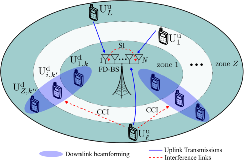
Figure 1: A small cell FD-NOMA MU-MISO system. FD-BS serves $M=ZK$ DL users, with $K$ DL users in each of $Z$ zones, and $L$ UL users which are assumed to be uniformly deployed in the cell.

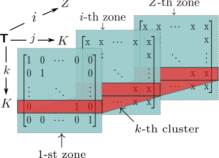
Figure 2: The structure of tensor T, representing the DL user association. The $i$-th plane containing matrix $\mathbf{C}_{i}\in\{0,1\}^{K\times K},\;i\in\mathcal{Z}$ indicates whether the $j$-th DL user in zone $i$ is assigned to the $k$-th cluster.

Consider a small cell in which the BS is equipped with $N>1$ antennas. To facilitate the NOMA operation, as in [31, 32, 9], the cell is virtually partitioned into $Z$ annular regions (or zones) whose channel conditions are as much different as possible. Specifically, we number the zones/regions of $\mathcal{Z}\triangleq\{1,2,\dots,Z\}$ in an ascending order with respect to their distance from the BS, i.e., the $1$-st and $Z$-th zones are the nearest and farthest zones, respectively. In practice, we do not know how many zones are chosen to provide the best performance, since it depends on different criteria, such as channel condition, cell size, the number of antennas and users. Finding the optimal number of zones is out of scope of this work. For the sake of mathematical convenience, we assume each zone contains $K$ DL users leading $M=ZK$ DL users in total (note that the following analysis is also applicable when zones have different numbers of DL users).

The BS is assumed to be equipped with FD capability, e.g., using the circulator-based FD radio prototypes [12] to simultaneously serve $M$ and $L$ single-antenna DL and UL users in the same frequency band, respectively. We denote the $k$-th DL user in zone $i$ by $\mathtt{U}_{ik}^{\mathtt{d}},\;\forall i\in\mathcal{Z},k\in\mathcal{K}\triangleq\{1,2,\dots,K\}$, while the $\ell$-th UL user at an arbitrary location is represented by $\mathtt{U}_{\ell}^{\mathtt{u}},\;\forall\ell\in\mathcal{L}\triangleq\{1,2,\dots,L\}$. The channel vectors from the BS to $\mathtt{U}_{ik}^{\mathtt{d}}$ and from $\mathtt{U}_{\ell}^{\mathtt{u}}$ to the BS are denoted by $\mathbf{h}_{ik}^{\mathtt{d}}\in\mathbb{C}^{N\times 1}$ and $\mathbf{h}_{\ell}^{\mathtt{u}}\in\mathbb{C}^{N\times 1}$, respectively. To capture the imperfect SiS at the BS, let $\mathbf{G}_{\mathtt{SI}}\in\mathbb{C}^{N\times N}$ and $\rho\in[0,1)$ be the SI channel matrix and the residual SiS level, respectively. Further, let $g_{\ell,ik}$ denote the CCI channel from $\mathtt{U}_{\ell}^{\mathtt{u}}$ to $\mathtt{U}_{ik}^{\mathtt{d}}$.

II-A Downlink Transmission

Before proceeding further, we first lay a foundation on third-order tensor to generalize the DL user clustering through the following definitions.

Definition 1

A group of DL users consisting of $Z$ DL users, in which no two DL users come from the same zone is called a cluster (of users). The NOMA beamforming is thus applied to $K$ different clusters. The third-order tensor $\textsf{{T}}\triangleq[T_{kji}]_{k,j\in\mathcal{K},i\in\mathcal{Z}}$ is used for user associations, where $T_{kji}\in\{0,1\}$. If $T_{kji}=1$, the $j$-th DL user in zone $i$ is admitted to the $k$-th cluster, and vice versa.

Definition 2

It can be foreseen that $K$ users in each zone will result in $K!$ possible permutations of clusters. To simplify the considered problem we utilize DL user indices in the first zone to index the clusters. In other words, the $k$-th DL user in the first zone is always admitted to the $k$-th cluster. As illustrated in Fig. 2, T is formed by $Z$ matrices w.r.t. the index $i$ as $\textsf{{T}}=\{\mathbf{C}_{i}\}_{i\in\mathcal{Z}}$, with $\mathbf{C}_{i}\triangleq\bigl{[}T_{kji}\bigr{]}_{k,j\in\mathcal{K}}\in\{0,1\}^{K\times K}$ representing the $i$-th zone, and thus the first matrix of T is assigned to the identity matrix, i.e., $\mathbf{C}_{1}\triangleq\bigl{[}T_{kj1}\bigr{]}=\mathbf{I}_{K}$. According to Definition 1, $\mathbf{C}_{i}$ with $i\in\mathcal{Z}\backslash\{1\}$ is considered as the association variables of DL users.

From the two definitions above, we now establish the UA between two arbitrary zones as follows.

Theorem 1

Let $\mathbf{T}^{iz}\in\{0,1\}^{K\times K},\;\forall i,z\in\mathcal{Z}$ be an UA matrix between zones $i$ and $z$. If the entry $T_{kj}^{iz},\;\forall k,j\in\mathcal{K}$ is set to 1, the $k$-th DL user in zone $i$ and the $j$-th DL user in zone $z$ are grouped into the same cluster, and vice versa. Based on the structure of T, the matrix $\mathbf{T}^{iz}$ is simply calculated as

$$\mathbf{T}^{iz}=\mathbf{C}_{i}^{T}\mathbf{C}_{z}.$$ (1)

Proof:

Please see Appendix A. ∎

In the DL channel, BS employs a linear beamforming vector $\mathbf{w}_{ik}\in\mathbb{C}^{N\times 1}$ to precode the data symbol $x_{ik}^{\mathtt{d}}$, with $\mathbb{E}\bigl{[}|x_{ik}^{\mathtt{d}}|^{2}\bigr{]}=1$, intended to $\mathtt{U}_{ik}^{\mathtt{d}}$. The received signal at $\mathtt{U}_{ik}^{\mathtt{d}}$ can be expressed as

$$y_{ik}^{\mathtt{d}}=\sum\nolimits_{i^{\prime}\in\mathcal{Z}}\sum\nolimits_{k^{\prime}\in\mathcal{K}}(\mathbf{h}_{ik}^{\mathtt{d}})^{H}\mathbf{w}_{i^{\prime}k^{\prime}}x_{i^{\prime}k^{\prime}}^{\mathtt{d}}+\underbrace{\sum\nolimits_{\ell\in\mathcal{L}}p_{\ell}g_{\ell,ik}x_{\ell}^{\mathtt{u}}}_{\text{CCI}}+n_{ik},$$ (2)

where $p_{\ell}$ and $x_{\ell}^{\mathtt{u}}$, with $\mathbb{E}\bigl{[}|x_{\ell}^{\mathtt{u}}|^{2}\bigr{]}=1$, are the transmit power coefficient and data symbol of $\mathtt{U}_{\ell}^{\mathtt{u}}$, respectively; and $n_{ik}\sim\mathcal{CN}(0,\sigma_{ik}^{2})$ is the additive white Gaussian noise (AWGN) at $\mathtt{U}_{ik}^{\mathtt{d}}$. The messages intended to DL user in cluster $k$ are sequentially decoded as follows. $\mathtt{U}_{ik}^{\mathtt{d}}$ first decodes the messages of $\mathtt{U}_{i^{\prime}j}^{\mathtt{d}}$ with $i^{\prime}\in\mathcal{Z}_{i}^{+}\triangleq\{i+1,\dots,Z\}$ for $T_{kj}^{ii^{\prime}}=1$, and then removes them by using the SIC technique before decoding its own message. The received signal-to-interference-plus-noise ratio (SINR) at $\mathtt{U}_{ik}^{\mathtt{d}}$ can be generally expressed as

$$\gamma_{ik}^{\mathtt{d}}(\mathbf{w},\mathbf{p},\textsf{{T}})=\underset{z\in\mathcal{Z}_{i}}{\min}\;\underset{j\in\mathcal{K}}{\max}\Biggl{\{}\mfrac{T_{jk}^{zi}|(\mathbf{h}_{zj}^{\mathtt{d}})^{H}\mathbf{w}_{ik}|^{2}}{\Theta_{jk}^{zi}(\mathbf{w},\mathbf{p},\textsf{{T}})}\Biggr{\}}$$

where $\mathcal{Z}_{i}\triangleq\{1,\dots,i\}$, $\mathbf{p}=[p_{\ell}]_{\ell\in\mathcal{L}}$, $\mathbf{w}=[\mathbf{w}_{i}^{H}]^{H}_{i\in\mathcal{Z}}$ with $\mathbf{w}_{i}\triangleq[\mathbf{w}_{ik}^{H}]_{k\in\mathcal{K}}^{H}$, and the interference-plus-noise (IN) for decoding the $\mathtt{U}_{ik}^{\mathtt{d}}$’s message at $\mathtt{U}_{zj}^{\mathtt{d}}$, denoted by $\Theta_{jk}^{zi}(\mathbf{w},\mathbf{p},\textsf{{T}})$, is given as

$$\Theta_{jk}^{zi}(\mathbf{w},\mathbf{p},\textsf{{T}})=\underset{(z^{\prime},j^{\prime})\neq(i,k)}{\sum_{z^{\prime}\in\mathcal{Z}_{i}}\;\sum_{j^{\prime}\in\mathcal{K}}}|(\mathbf{h}_{zj}^{\mathtt{d}})^{H}\mathbf{w}_{z^{\prime}j^{\prime}}|^{2}+\sum_{i^{\prime}\in\mathcal{Z}_{i}^{+}}\sum_{k^{\prime}\in\mathcal{K}}(1-T_{jk^{\prime}}^{zi^{\prime}})|(\mathbf{h}_{zj}^{\mathtt{d}})^{H}\mathbf{w}_{i^{\prime}k^{\prime}}|^{2}+\sum_{\ell\in\mathcal{L}}p_{\ell}^{2}|g_{\ell,zj}|^{2}+\sigma_{zj}^{2}.\quad\;$$ (3)

II-B Uplink Transmission

The received signal vector at the FD-BS in the UL transmission can be expressed as

$$\mathbf{y}^{\mathtt{u}} =\sum\nolimits_{\ell\in\mathcal{L}}p_{\ell}\mathbf{h}_{\ell}^{\mathtt{u}}x_{\ell}^{\mathtt{u}}+\underbrace{\rho\sum\nolimits_{i\in\mathcal{Z}}\sum\nolimits_{k\in\mathcal{K}}\mathbf{G}_{\mathtt{SI}}^{H}\mathbf{w}_{ik}x_{ik}^{\mathtt{d}}}_{\text{SI}}+\mathbf{n},$$ (4)

where $\mathbf{n}\sim\mathcal{CN}(0,\sigma_{\mathtt{U}}^{2}\mathbf{I})$ is the AWGN. To decode the UL messages, we adopt the minimum mean-square error and SIC (MMSE-SIC) decoder at the FD-BS [35]. To jointly optimize the UL users’ decoding order, we introduce binary variables $\beta_{\ell m}\in\{0,1\},\forall\ell,m\in\mathcal{L}$. Specifically, the message of the $\ell$-th UL user is successfully decoded prior to that of the $m$-th UL user if $\beta_{\ell m}=1$ in sync with $\beta_{m\ell}=0$, and they are in reverse order if $\beta_{\ell m}=0$. On this basis and by treating the residual SiS as noise, the received SINR of $\mathtt{U}_{\ell}^{\mathtt{u}}$ at the FD-BS can be expressed as

$$\gamma_{\ell}^{\mathtt{u}}\bigl{(}\mathbf{w},\mathbf{p},\boldsymbol{\beta}\bigr{)}=p_{\ell}^{2}(\mathbf{h}_{\ell}^{\mathtt{u}})^{H}\bigl{(}\boldsymbol{\Psi}_{\ell}(\mathbf{w},\mathbf{p},\boldsymbol{\beta})\bigr{)}^{-1}\mathbf{h}_{\ell}^{\mathtt{u}},$$ (5)

where $\boldsymbol{\beta}\triangleq[\beta_{\ell m}]_{\ell,m\in\mathcal{L}}$ and

$$\boldsymbol{\Psi}_{\ell}(\mathbf{w},\mathbf{p},\boldsymbol{\beta})\triangleq\sum\nolimits_{m\in\mathcal{L}}\beta_{\ell m}p_{m}^{2}\mathbf{h}_{m}^{\mathtt{u}}(\mathbf{h}_{m}^{\mathtt{u}})^{H}+\rho^{2}\sum\nolimits_{i\in\mathcal{Z}}\sum\nolimits_{k\in\mathcal{K}}\mathbf{G}_{\mathtt{SI}}^{H}\mathbf{w}_{ik}\mathbf{w}_{ik}^{H}\mathbf{G}_{\mathtt{SI}}+\sigma_{\mathtt{U}}^{2}\mathbf{I}.$$

II-C Optimization Problem Formulation

With the above discussion, the achievable rates (measured in nats/s/Hz) of $\mathtt{U}_{ik}^{\mathtt{d}}$ and $\mathtt{U}_{\ell}^{\mathtt{u}}$ are respectively given as

$$R_{ik}^{\mathtt{d}}\bigl{(}\mathbf{w},\mathbf{p},\textsf{{T}}\bigr{)} =\ln\bigl{(}1+\gamma_{ik}^{\mathtt{d}}(\mathbf{w},\mathbf{p},\textsf{{T}})\bigr{)},$$ (6)

$$R_{\ell}^{\mathtt{u}}\bigl{(}\mathbf{w},\mathbf{p},\boldsymbol{\beta}\bigr{)} =\ln\bigl{(}1+\gamma_{\ell}^{\mathtt{u}}(\mathbf{w},\mathbf{p},\boldsymbol{\beta})\bigr{)}.$$ (7)

Herein, our main goal is to jointly optimize beamformers and transmit power ($\mathbf{w},\mathbf{p}$) and binary variables $(\textsf{{T}},\boldsymbol{\beta})$, so that the total SE is maximized subject to QoS and power constraints. We can now state the SE maximization problem, referred to as SEM problem for short, as

$$\underset{\mathbf{w},\mathbf{p},\textsf{{T}},\boldsymbol{\beta}}{\max} \ R_{\Sigma}\triangleq\sum\nolimits_{i\in\mathcal{Z}}\sum\nolimits_{k\in\mathcal{K}}R_{ik}^{\mathtt{d}}\bigl{(}\mathbf{w},\mathbf{p},\textsf{{T}}\bigr{)}+\sum\nolimits_{\ell\in\mathcal{L}}R_{\ell}^{\mathtt{u}}\bigl{(}\mathbf{w},\mathbf{p},\boldsymbol{\beta}\bigr{)}$$ (8a)

$${\mathrm{s.t.}} \;\|\mathbf{w}\|^{2}\leq P_{\mathtt{bs}}^{\text{max}},$$ (8b)

$$p_{\ell}^{2}\leq P_{\ell}^{\text{max}},\;p_{\ell}\geq 0,\ \forall\ell\in\mathcal{L},$$ (8c)

$$R_{ik}^{\mathtt{d}}\bigl{(}\mathbf{w},\mathbf{p},\textsf{{T}}\bigr{)}\geq\bar{R}_{ik}^{\mathtt{d}},\;\forall i\in\mathcal{Z},\;k\in\mathcal{K},$$ (8d)

$$R_{\ell}^{\mathtt{u}}\bigl{(}\mathbf{w},\mathbf{p},\boldsymbol{\beta}\bigr{)}\geq\bar{R}_{\ell}^{\mathtt{u}},\;\forall\ell\in\mathcal{L},$$ (8e)

$$T_{kj}^{iz}\in\{0,1\},\;\forall i,z\in\mathcal{Z},\;\forall k,j\in\mathcal{K},$$ (8f)

$$\sum\nolimits_{k\in\mathcal{K}}T_{kj}^{iz}=1,\;\sum\nolimits_{j\in\mathcal{K}}T_{kj}^{iz}=1,\forall i,z\in\mathcal{Z},\ \forall k,j\in\mathcal{K},\;$$ (8g)

$$\beta_{\ell m}\in\{0,1\},\;\forall\ell,m\in\mathcal{L},$$ (8h)

$$\beta_{\ell\ell}=0,\;\forall\ell\in\mathcal{L},$$ (8i)

$$\beta_{\ell m}+\beta_{m\ell}=1,\;\ell\neq m,\;\forall\ell,m\in\mathcal{L},$$ (8j)

$$\bigl{|}\sum\nolimits_{m\in\mathcal{L}}\beta_{\ell m}-\sum\nolimits_{m\in\mathcal{L}}\beta_{\ell^{\prime}m}\bigr{|}\geq 1,\;\ell\neq\ell^{\prime},\;\forall\ell,\ell^{\prime}\in\mathcal{L},$$ (8k)

where $P_{\mathtt{bs}}^{\text{max}}$ and $P_{\ell}^{\text{max}}$ in (8b) and (8c) are the transmit power budgets at the BS and $\mathtt{U}_{\ell}^{\mathtt{u}}$, respectively. In (8d) and (8e), we impose the minimum QoS requirements $\bar{R}_{ik}^{\mathtt{d}}\geq 0$ and $\bar{R}_{\ell}^{\mathtt{u}}\geq 0$ in order to maintain some degree of fairness among users. Constraints (8f) and (8g) establish the criteria for DL user clustering, in which $\mathbf{T}^{iz}$ satisfies the property of tensor T given in Theorem 1, while constraints (8h)-(8k) determine the decoding orders of UL users. Due to the non-concavity of the objective (8a) and the non-convexity of QoS constraints w.r.t. the decision variables (i.e., by examining the Hessian matrix), problem (8) belongs to a class of mixed-integer non-convex problem.

Remark 1

The merits of Theorem 1 to problem (8) are as follows. First, the search region for DL user clustering via tensor T is significantly reduced compared to the exhaustive search method, since $\mathbf{C}_{1}$ is fixed to identity matrix. Accordingly, the association problem avoids searching all permutations of clusters while still achieving a close-to-optimal solution. The second advantage is to reduce the number of association variables. For NOMA decoding at a certain zone, the knowledge of UA with other zones is required, i.e., $K^{2}$ variables for each of ${2\choose Z}$ couples of zones, leading to ${2\choose Z}K^{2}$ UA variables required zone-by-zone. In comparison, by exploiting the tensor structure of T, the number of decision variables for user clustering is significantly reduced to $(Z-1)K^{2}$. Finally, the association among DL users is properly defined by Theorem 1, in which the tensor T storing the change-of-basis matrices w.r.t. the identity-matrix basis is sufficient to recover the UA matrix of any two zones via (1). Note that $T_{kji}$ is an element of T, while $T_{kj}^{iz}$ is an entry of the matrix $\mathbf{T}^{iz}$ derived from (1). From the fact that $\mathbf{C}_{1}=\mathbf{I}_{K}$ as in Definition 2, $\mathbf{C}_{i},i\in\mathcal{Z}\backslash\{1\}$ becomes the UA matrix between zone 1 and zone $i$, leading to $\mathbf{T}^{1i}\equiv\mathbf{C}_{i}$. When zones have different numbers of DL users, let us denote the number of users in zone $z$ by $K_{z},\;z\in\mathcal{Z}\triangleq\{1,\dots,Z\}$. If $K_{z}<K\triangleq\underset{z\in\mathcal{Z}}{\max}\{K_{z}\}$, some new users with zero channel vectors can be added to zone $z$, such that each zone has $K$ DL users. The third-order tensor remains unchanged. Accordingly, problem (8) can be easily re-expressed by forcing beamforming vectors of newly added users to be zeros and skipping their QoS constraints.

Remark 2

As pointed out in [32], a larger cluster size with more distinct channel conditions among DL users is more desirable. This is because a large size of a DL cluster with very different channel gains plays a vital role in NOMA systems. This mainly depends on the number of DL users and cell size. In this paper, we focus on a small-cell setup, which is merely due to current practical limitations of FD radios [15, 16, 17, 18, 19, 20]. As such, it is reasonable to consider a two-zone NOMA for FD small-cell systems, as in the following case study.

Case study with $Z=2$: To reduce the system load and processing delay, we will study user pairing for DL transmission, where NOMA is applied to pairs of two DL users. Here, each pair includes one near DL user $\mathtt{U}_{1k}^{\mathtt{d}}$ in the inner zone and one far DL user $\mathtt{U}_{2j}^{\mathtt{d}}$ in the outer zone. We should note that the two-zone NOMA for DL transmission has been widely adopted in the literature [32, 19, 31]. In this case, T includes two UA matrices as $\mathbf{C}_{1}=\mathbf{I}_{K}$ and $\mathbf{C}_{2}\in\{0,1\}^{K\times K}$. Without loss of generality, let $\boldsymbol{\alpha}=\mathbf{T}^{12}=\mathbf{C}_{2}$ be a unique matrix of UA variables in T, and then the entries of $\boldsymbol{\alpha}$ are $\alpha_{kj}\in\{0,1\}$, indicating whether $\mathtt{U}_{1k}^{\mathtt{d}}$ in zone 1 is paired with $\mathtt{U}_{2j}^{\mathtt{d}}$ in zone 2. From (II-A), the SINRs at $\mathtt{U}_{1k}^{\mathtt{d}}$ and $\mathtt{U}_{2j}^{\mathtt{d}}$ are respectively simplified as

$$\gamma_{1k}^{\mathtt{d}}(\mathbf{w},\mathbf{p},\boldsymbol{\alpha}) =\mfrac{|(\mathbf{h}_{1k}^{\mathtt{d}})^{H}\mathbf{w}_{1k}|^{2}}{\phi_{k}(\mathbf{w},\mathbf{p},\boldsymbol{\alpha})},$$ (9a)

$$\gamma_{2j}^{\mathtt{d}}(\mathbf{w},\mathbf{p},\boldsymbol{\alpha}) =\min\Biggl{\{}\underset{k\in\mathcal{K}}{\max}\Bigl{\{}\mfrac{\alpha_{kj}|(\mathbf{h}_{1k}^{\mathtt{d}})^{H}\mathbf{w}_{2j}|^{2}}{\psi_{j}^{k}(\mathbf{w},\mathbf{p})}\Bigr{\}},\mfrac{|(\mathbf{h}_{2j}^{\mathtt{d}})^{H}\mathbf{w}_{2j}|^{2}}{\varphi_{j}(\mathbf{w},\mathbf{p})}\Biggr{\}},$$ (9b)

where the IN $\phi_{k}(\mathbf{w},\mathbf{p},\boldsymbol{\alpha})$ experienced by $\mathtt{U}_{1k}^{\mathtt{d}}$ is

$$\phi_{k}(\mathbf{w},\mathbf{p},\boldsymbol{\alpha})=\sum\nolimits_{k^{\prime}\in\mathcal{K}\setminus k}|(\mathbf{h}_{1k}^{\mathtt{d}})^{H}\mathbf{w}_{1k^{\prime}}|^{2}+\sum\nolimits_{\ell\in\mathcal{L}}p_{\ell}^{2}|g_{\ell,1k}|^{2}+\sum\nolimits_{j^{\prime}\in\mathcal{K}}(1-\alpha_{kj^{\prime}})|(\mathbf{h}_{1k}^{\mathtt{d}})^{H}\mathbf{w}_{2j^{\prime}}|^{2}+\sigma_{1k}^{2},$$

while the INs involved in the SINRs for decoding the $\mathtt{U}_{2j}^{\mathtt{d}}$’s message at $\mathtt{U}_{1k}^{\mathtt{d}}$ and itself, denoted by $\psi_{j}^{k}(\mathbf{w},\mathbf{p})$ and $\varphi_{j}(\mathbf{w},\mathbf{p})$, are respectively given as

$$\psi_{j}^{k}(\mathbf{w},\mathbf{p})= \sum\nolimits_{k^{\prime}\in\mathcal{K}}|(\mathbf{h}_{1k}^{\mathtt{d}})^{H}\mathbf{w}_{1k^{\prime}}|^{2}+\sum\nolimits_{j^{\prime}\in\mathcal{K}\setminus j}|(\mathbf{h}_{1k}^{\mathtt{d}})^{H}\mathbf{w}_{2j^{\prime}}|^{2}+\sum\nolimits_{\ell\in\mathcal{L}}p_{\ell}^{2}|g_{\ell,1k}|^{2}+\sigma_{1k}^{2},$$

$$\varphi_{j}(\mathbf{w},\mathbf{p})= \sum\nolimits_{k^{\prime}\in\mathcal{K}}|(\mathbf{h}_{2j}^{\mathtt{d}})^{H}\mathbf{w}_{1k^{\prime}}|^{2}+\sum\nolimits_{j^{\prime}\in\mathcal{K}\setminus j}|(\mathbf{h}_{2j}^{\mathtt{d}})^{H}\mathbf{w}_{2j^{\prime}}|^{2}+\sum\nolimits_{\ell\in\mathcal{L}}p_{\ell}^{2}|g_{\ell,2j}|^{2}+\sigma_{2j}^{2}.$$

We remark that the first term in (9b) is the SINR for decoding the $\mathtt{U}_{2j}^{\mathtt{d}}$’s message at $\mathtt{U}_{1k}^{\mathtt{d}}$, which is imposed on $\gamma_{2j}^{\mathtt{d}}(\mathbf{w},\mathbf{p},\boldsymbol{\alpha})$ to ensure that $\mathtt{U}_{1k}^{\mathtt{d}}$ can successfully decode the $\mathtt{U}_{2j}^{\mathtt{d}}$’s message by SIC [32, 28]. Toward this end, we consider the following modified problem of (8)

$$\underset{\mathbf{w},\mathbf{p},\boldsymbol{\alpha},\boldsymbol{\beta}}{\max} \;R_{\Sigma}\triangleq\sum\nolimits_{i\in\mathcal{Z}}\sum\nolimits_{k\in\mathcal{K}}R_{ik}^{\mathtt{d}}\bigl{(}\mathbf{w},\mathbf{p},\boldsymbol{\alpha}\bigr{)}+\sum\nolimits_{\ell\in\mathcal{L}}R_{\ell}^{\mathtt{u}}\bigl{(}\mathbf{w},\mathbf{p},\boldsymbol{\beta}\bigr{)}\qquad\;$$ (10a)

$${\mathrm{s.t.}} \;\eqref{eq: prob. general form tensor :: b},\eqref{eq: prob. general form tensor :: c},\eqref{eq: prob. general form tensor :: f},\eqref{eq: prob. general form tensor :: j}-\eqref{eq: prob. general form tensor :: m},$$ (10b)

$$\;R_{ik}^{\mathtt{d}}\bigl{(}\mathbf{w},\mathbf{p},\boldsymbol{\alpha}\bigr{)}\geq\bar{R}_{ik}^{\mathtt{d}},\;\forall i\in\mathcal{Z},k\in\mathcal{K},$$ (10c)

$$\;\alpha_{kj}\in\{0,1\},\;\forall k,j\in\mathcal{K},$$ (10d)

$$\;\sum\nolimits_{k\in\mathcal{K}}\alpha_{kj}=1,\;\sum\nolimits_{j\in\mathcal{K}}\alpha_{kj}=1,\forall k,j\in\mathcal{K}.$$ (10e)

where $R_{ik}^{\mathtt{d}}\bigl{(}\mathbf{w},\mathbf{p},\boldsymbol{\alpha}\bigr{)}$, is derived by replacing $\gamma_{ik}^{\mathtt{d}}(\mathbf{w},\mathbf{p},\textsf{{T}})$ in (6) with $\gamma_{ik}^{\mathtt{d}}(\mathbf{w},\mathbf{p},\boldsymbol{\alpha})$ given by (9). In what follows, three iterative algorithms to solve the SEM problem (10) will be presented. However, the mathematical presentation can be slightly modified to address the general SEM problem (8), and numerical results for the three-zone NOMA scenario will be elaborated in Section VI.

In this paper, we focus on slowly time-varying channels in small cell systems and adopt the channel reciprocity of UL and DL channels in time division duplex (TDD) mode. At the beginning of each time block, BS obtains the CSI of DL and UL channels by requesting all users to simultaneously transmit mutually orthogonal pilot sequences of length $\tau$ symbols (i.e., $\tau\geq M+L$). Generally, the pilots are transmitted via public channel and the framework of training sequence can be known at UL users. Therefore, for the acquisition of the CSI of CCI channels, UL users can take advantage of the pilots sent from DL users and then estimate CCI channels through TDD. Then, during the transmission phase, the estimated CCI channels acquired by the BS can be periodically embedded in the data packets of UL users. For slowly time-varying channels, it is reasonable to assume that the CSI of all links in the network is available at the BS, where the system optimization is carried out. The performance under perfect CSI unveils an upper bound for the achievement of FD-NOMA systems.

III Proposed Suboptimal Designs

In general, finding a globally optimal solution to (10) is very challenging due to two obvious reasons. First, solving problem (10) for an optimal solution may end up with an exhaustive search due to the strong coupling between the continuous variables $(\mathbf{w},\mathbf{p})$ and binary variables $(\boldsymbol{\alpha},\boldsymbol{\beta})$. Second, even if the binary variables are fixed, problem (10) still remains highly non-convex in the continuous variables. This method is of little practical use in wireless communication designs since the resulting computational complexity grows exponentially when the number of users increases. This motivates us to develop more practically appealing methods which can find a good solution with much less complexity. In particular, we first relax the binary UA variables to tackle the binary nature of the problem (10), and then, two suboptimal low-complexity algorithms are proposed to solve the resulting non-convex CR problem. In the first algorithm, we employ the ICA framework [33, 34] to convexify the non-convex continuous parts, which aims at finding the approximate, but efficient solution to the CR problem. In the second algorithm, we propose an approach combining ICA and penalty method to produce a higher quality solution.

III-A ICA-CR based Design

We first consider the following CR of problem (10)

$$\underset{\mathbf{w},\mathbf{p},\boldsymbol{\alpha},\boldsymbol{\beta}}{\max} \quad\sum\nolimits_{i\in\mathcal{Z}}\sum\nolimits_{k\in\mathcal{K}}R_{ik}^{\mathtt{d}}\bigl{(}\mathbf{w},\mathbf{p},\boldsymbol{\alpha}\bigr{)}+\sum\nolimits_{\ell\in\mathcal{L}}R_{\ell}^{\mathtt{u}}\bigl{(}\mathbf{w},\mathbf{p},\boldsymbol{\beta}\bigr{)}\quad\quad$$ (11a)

$${\mathrm{s.t.}} \quad\eqref{eq: prob. general form tensor :: b},\eqref{eq: prob. general form tensor :: c},\eqref{eq: prob. general form tensor :: f},\eqref{eq: prob. general form tensor :: k}-\eqref{eq: prob. general form tensor :: m},\eqref{eq: prob. general form c},\eqref{eq: prob. general form e},$$ (11b)

$$\quad 0\leq\alpha_{kj}\leq 1,\;\forall k,j\in\mathcal{K},$$ (11c)

$$\quad 0\leq\beta_{\ell m}\leq 1,\;\forall\ell,m\in\mathcal{L},$$ (11d)

where $\boldsymbol{\alpha}$ and $\boldsymbol{\beta}$ are relaxed to be continuous as in (11c) and (11d), respectively. By following the relaxation property, the feasible region of (11) is larger than that of (10), and thus any feasible point of the latter is also feasible for the former. It is obvious that the difficulty in solving problem (11) is due to the non-concave objective (11a) and non-convex constraints in (8e), (8k) and (10c). In light of the ICA method, convex approximations are required to tackle the non-convexity of (11).

Concavity of the objective (11a): Let us start by handling the non-concavity of $R_{ik}^{\mathtt{d}}(\mathbf{w},\mathbf{p},\boldsymbol{\alpha})$. For $\mathtt{U}_{1k}^{\mathtt{d}}$ (DL users in zone 1), we introduce new variables $\omega_{1k},\forall k\in\mathcal{K}$ to explicitly expose the non-convex parts of $R_{1k}^{\mathtt{d}}(\mathbf{w},\mathbf{p},\boldsymbol{\alpha})$ as

$$R_{1k}^{\mathtt{d}}(\mathbf{w},\mathbf{p},\boldsymbol{\alpha}) \geq\ln\bigl{(}1+\mfrac{1}{\omega_{1k}}\bigr{)},$$ (12a)

$$\mfrac{|(\mathbf{h}_{1k}^{\mathtt{d}})^{H}\mathbf{w}_{1k}|^{2}}{\phi_{k}(\mathbf{w},\mathbf{p},\boldsymbol{\alpha})} \geq\mfrac{1}{\omega_{1k}},$$ (12b)

which does not affect the optimality. The reason is that (12b) must hold with equality at the optimum; otherwise, we can decrease $\omega_{1k}$ to obtain a higher objective without violating the constraint. We are now ready to use ICA for approximating (12). Suppose the value of $x$ at iteration $\kappa$ in the proposed iterative algorithm is denoted by $x^{(\kappa)}$, which is referred as a feasible point of $x$ at iteration $\kappa+1$. From (12a) and as an effort to reduce the complexity of log function, the concave minorant of $R_{1k}^{\mathtt{d}}(\mathbf{w},\mathbf{p},\boldsymbol{\alpha})$ at the $(\kappa+1)$-th iteration is derived as

$$R_{1k}^{\mathtt{d}}(\mathbf{w},\mathbf{p},\boldsymbol{\alpha})\geq\mathtt{A}(\omega_{1k}^{(\kappa)})+\mathtt{B}(\omega_{1k}^{(\kappa)})\omega_{1k}:=\ddot{R}_{1k}^{\mathtt{d},(\kappa)},$$ (13)

due to the convexity of $\ln\bigl{(}1+\mfrac{1}{\omega_{1k}}\bigr{)},$ where $\mathtt{A}(\omega_{1k}^{(\kappa)})\triangleq\ln\bigl{(}1+\mfrac{1}{\omega_{1k}^{(\kappa)}}\bigr{)}+\mfrac{1}{(\omega_{1k}^{(\kappa)}+1)}$ and $\mathtt{B}(\omega_{1k}^{(\kappa)})\triangleq-\mfrac{1}{\omega_{1k}^{(\kappa)}(\omega_{1k}^{(\kappa)}+1)}$ [32, Eq. (82)]. It is obvious that the equality in (13) holds true whenever $\omega_{1k}=\omega_{1k}^{(\kappa)}$. In other words, we obtain $R_{1k}^{\mathtt{d}}(\mathbf{w},\mathbf{p},\boldsymbol{\alpha})=\ddot{R}_{1k}^{\mathtt{d},(\kappa)}$ as $\kappa\rightarrow\infty$. By applying the ICA method, we iteratively replace the non-convex constraint (12b) by

$$\phi_{k}(\mathbf{w},\mathbf{p},\boldsymbol{\alpha})\leq\omega_{1k}\tilde{\gamma}_{1k}^{(\kappa)}\bigl{(}\mathbf{w}\bigr{)},$$ (14)

over the trust region (i.e., the feasible domain):

$$\tilde{\gamma}_{1k}^{(\kappa)}(\mathbf{w})\triangleq\;2\Re\{(\mathbf{h}_{1k}^{\mathtt{d}})^{H}\mathbf{w}_{1k}^{(\kappa)}\}\Re\{(\mathbf{h}_{1k}^{\mathtt{d}})^{H}\mathbf{w}_{1k}\}-\bigl{(}\Re\{(\mathbf{h}_{1k}^{\mathtt{d}})^{H}\mathbf{w}_{1k}^{(\kappa)}\}\bigr{)}^{2}>0,\;\forall k\in\mathcal{K},$$ (15)

where $\tilde{\gamma}_{1k}^{(\kappa)}(\mathbf{w})$ is the first order approximation of $|(\mathbf{h}_{1k}^{\mathtt{d}})^{H}\mathbf{w}_{1k}|^{2}$ around the point $\mathbf{w}_{1k}^{(\kappa)}$ found at iteration $\kappa$. It can be seen that (14) is still a non-convex constraint due to non-convexity in the third term of function $\phi_{k}(\mathbf{w},\mathbf{p},\boldsymbol{\alpha})$. To overcome this issue, we introduce the following lemma.

Lemma 1

Consider a function $h(x,y)\triangleq xy^{2},\;x>0$. The convex majorant of $h(x,y)$ is expressed as

$$h(x,y)\leq\tilde{h}(x,z)\triangleq xz\leq\mfrac{z^{(\kappa)}}{2x^{(\kappa)}}x^{2}+\mfrac{x^{(\kappa)}}{2z^{(\kappa)}}z^{2}\triangleq\tilde{h}^{(\kappa)}(x,z),$$ (16)

by imposing an SOC constraint: $y^{2}\leq z$, where $z>0$ is a new variable.

Proof:

Please see Appendix B. ∎

By applying Lemma 1, the convex upper bound of $\phi_{k}(\mathbf{w},\mathbf{p},\boldsymbol{\alpha})$ is

$$\phi_{k}(\mathbf{w},\mathbf{p},\boldsymbol{\alpha}) \leq\sum_{k^{\prime}\in\mathcal{K}\setminus k}|(\mathbf{h}_{1k}^{\mathtt{d}})^{H}\mathbf{w}_{1k^{\prime}}|^{2}+\sum_{\ell\in\mathcal{L}}p_{\ell}^{2}|g_{\ell,1k}|^{2}+\sum_{j^{\prime}\in\mathcal{K}}\tilde{h}^{(\kappa)}(\lambda_{kj^{\prime}},\mu_{kj^{\prime}})+\sigma_{1k}^{2}:=\tilde{\phi}_{k}^{(\kappa)}(\mathbf{w},\mathbf{p},\boldsymbol{\lambda},\boldsymbol{\mu}),$$

where $\boldsymbol{\lambda}\triangleq[\lambda_{kj}]_{k,j\in\mathcal{K}}$ and $\boldsymbol{\mu}\triangleq[\mu_{kj}]_{k,j\in\mathcal{K}}$ are alternative variables, in which $\lambda_{kj}$ and $\mu_{kj}$ satisfy the following convex constraints:

$$\lambda_{kj} =1-\alpha_{kj},\;\forall k,j\in\mathcal{K},$$ (17a)

$$|(\mathbf{h}_{1k}^{\mathtt{d}})^{H}\mathbf{w}_{2j}|^{2} \leq\mu_{kj},\;\;\forall k,j\in\mathcal{K}.$$ (17b)

In this regard, we iteratively replace (14) by the convex constraint:

$$\tilde{\phi}_{k}^{(\kappa)}(\mathbf{w},\mathbf{p},\boldsymbol{\lambda},\boldsymbol{\mu})\leq\omega_{1k}\tilde{\gamma}_{1k}^{(\kappa)}\bigl{(}\mathbf{w}\bigr{)},\;\forall k\in\mathcal{K},$$ (18)

which is the SOC representative. To address $R_{2j}^{\mathtt{d}}(\mathbf{w},\mathbf{p},\boldsymbol{\alpha})$ (DL users in zone 2), we can equivalently express the SINR $\gamma_{2j}^{\mathtt{d}}$ of $\mathtt{U}_{2j}^{\mathtt{d}}$ as

$$\gamma_{2j}^{\mathtt{d}}(\mathbf{w},\mathbf{p},\boldsymbol{\alpha})=\min\Biggl{\{}\underset{k\in\mathcal{K}}{\min}\Bigl{\{}\mfrac{|(\mathbf{h}_{1k}^{\mathtt{d}})^{H}\mathbf{w}_{2j}|^{2}}{\alpha_{kj}\psi_{j}^{k}(\mathbf{w},\mathbf{p})}\Bigr{\}},\mfrac{|(\mathbf{h}_{2j}^{\mathtt{d}})^{H}\mathbf{w}_{2j}|^{2}}{\varphi_{j}(\mathbf{w},\mathbf{p})}\Biggr{\}}.$$ (19)

Note that $\underset{k\in\mathcal{K}}{\max}\Bigl{\{}\mfrac{\alpha_{kj}|(\mathbf{h}_{1k}^{\mathtt{d}})^{H}\mathbf{w}_{2j}|^{2}}{\psi_{j}^{k}(\mathbf{w},\mathbf{p})}\Bigr{\}}=\underset{k\in\mathcal{K}}{\min}\Bigl{\{}\mfrac{|(\mathbf{h}_{1k}^{\mathtt{d}})^{H}\mathbf{w}_{2j}|^{2}}{\alpha_{kj}\psi_{j}^{k}(\mathbf{w},\mathbf{p})}\Bigr{\}}$ at the optimality due to the inverse function of $\alpha_{kj}$. We replace $\alpha_{kj}$ by $\alpha_{kj}+\varepsilon$ to avoid the numerical problem design when $\alpha_{kj}=0$, where $\varepsilon$ is a given small number. In the same manner to (13), the non-smoothness and non-concavity of $R_{2j}^{\mathtt{d}}(\mathbf{w},\mathbf{p},\boldsymbol{\alpha})$ are tackled as

$$R_{2j}^{\mathtt{d}}(\mathbf{w},\mathbf{p},\boldsymbol{\alpha}) \geq\ln\Bigl{(}1+\mfrac{1}{\omega_{2j}}\Bigr{)}\geq\mathtt{A}(\omega_{2j}^{(\kappa)})+\mathtt{B}(\omega_{2j}^{(\kappa)})\omega_{2j}:=\ddot{R}_{2j}^{\mathtt{d},(\kappa)},$$ (20)

by imposing the following constraints

$$\mfrac{|(\mathbf{h}_{1k}^{\mathtt{d}})^{H}\mathbf{w}_{2j}|^{2}}{(\alpha_{kj}+\varepsilon)\psi_{j}^{k}(\mathbf{w},\mathbf{p})} \geq\mfrac{1}{\omega_{2j}},$$ (21a)

$$\mfrac{|(\mathbf{h}_{2j}^{\mathtt{d}})^{H}\mathbf{w}_{2j}|^{2}}{\varphi_{j}(\mathbf{w},\mathbf{p})} \geq\mfrac{1}{\omega_{2j}}.$$ (21b)

As in (12b), the non-convex constraints (21a) and (21b) are innerly convexified by

$$\psi_{j}^{k}(\mathbf{w},\mathbf{p}) \leq\omega_{2j}\ddot{\gamma}_{2,kj}^{(\kappa)}\bigl{(}\mathbf{w},\boldsymbol{\alpha}\bigr{)},\;\forall k,j\in\mathcal{K},$$ (22a)

$$\varphi_{j}(\mathbf{w},\mathbf{p}) \leq\omega_{2j}\tilde{\gamma}_{2j}^{(\kappa)}\bigl{(}\mathbf{w}\bigr{)},\;\forall j\in\mathcal{K},$$ (22b)

over the trust regions:

$$\ddot{\gamma}_{2,kj}^{(\kappa)}(\mathbf{w},\boldsymbol{\alpha})\triangleq \;\mfrac{2\Re\bigl{\{}\bigl{(}(\mathbf{h}_{1k}^{\mathtt{d}})^{H}\mathbf{w}_{2j}^{(\kappa)}\bigr{)}^{*}\bigl{(}(\mathbf{h}_{1k}^{\mathtt{d}})^{H}\mathbf{w}_{2j}\bigr{)}\bigr{\}}}{\alpha_{kj}^{(\kappa)}+\varepsilon}-\mfrac{|(\mathbf{h}_{1k}^{\mathtt{d}})^{H}\mathbf{w}_{2j}^{(\kappa)}|^{2}}{(\alpha_{kj}^{(\kappa)}+\varepsilon)^{2}}(\alpha_{kj}+\varepsilon)>0,\;\forall k,j\in\mathcal{K},$$ (23a)

$$\tilde{\gamma}_{2j}^{(\kappa)}(\mathbf{w})\triangleq \;2\Re\{(\mathbf{h}_{2j}^{\mathtt{d}})^{H}\mathbf{w}_{2j}^{(\kappa)}\}\Re\{(\mathbf{h}_{2j}^{\mathtt{d}})^{H}\mathbf{w}_{2j}\}-\bigl{(}\Re\{(\mathbf{h}_{2j}^{\mathtt{d}})^{H}\mathbf{w}_{2j}^{(\kappa)}\}\bigr{)}^{2}>0,\;\forall j\in\mathcal{K}.$$ (23b)

Next, at the feasible point $(\mathbf{w}^{(\kappa)},\mathbf{p}^{(\kappa)},\boldsymbol{\beta}^{(\kappa)})$, the UL rate $R_{\ell}^{\mathtt{u}}\bigl{(}\mathbf{w},\mathbf{p},\boldsymbol{\beta}\bigr{)}$ is globally lower bounded by

$$R_{\ell}^{\mathtt{u}}(\mathbf{w},\mathbf{p},\boldsymbol{\beta})\geq\tilde{\mathtt{A}}\bigl{(}\gamma_{\ell}^{\mathtt{u}}\bigl{(}\mathbf{w}^{(\kappa)},\mathbf{p}^{(\kappa)},\boldsymbol{\beta}^{(\kappa)}\bigr{)}\bigr{)}-\Phi_{\ell}^{(\kappa)}(\mathbf{w},\mathbf{p},\boldsymbol{\beta})+\mfrac{2\gamma_{\ell}^{\mathtt{u}}\bigl{(}\mathbf{w}^{(\kappa)},\mathbf{p}^{(\kappa)},\boldsymbol{\beta}^{(\kappa)}\bigr{)}}{p_{\ell}^{(\kappa)}}p_{\ell},$$ (24)

where

$$\tilde{\mathtt{A}}\bigl{(}\gamma_{\ell}^{\mathtt{u}}(\mathbf{w}^{(\kappa)},\mathbf{p}^{(\kappa)},\boldsymbol{\beta}^{(\kappa)})\bigr{)}\triangleq\ln\bigl{(}1+\gamma_{\ell}^{\mathtt{u}}(\mathbf{w}^{(\kappa)},\mathbf{p}^{(\kappa)},\boldsymbol{\beta}^{(\kappa)})\bigr{)}-\gamma_{\ell}^{\mathtt{u}}(\mathbf{w}^{(\kappa)},\mathbf{p}^{(\kappa)},\boldsymbol{\beta}^{(\kappa)}),$$

$$\Phi_{\ell}^{(\kappa)}(\mathbf{w},\mathbf{p},\boldsymbol{\beta})\triangleq p_{\ell}^{2}\Lambda_{\ell}+\sum\nolimits_{m\in\mathcal{L}\setminus\ell}\beta_{\ell m}p_{m}^{2}\Lambda_{m}+\rho^{2}\sum\nolimits_{k\in\mathcal{K}}\bigl{(}\mathbf{w}_{k}\bigr{)}^{H}\mathbf{G}_{\mathtt{SI}}\boldsymbol{\Xi}_{\ell}^{(\kappa)}\mathbf{G}_{\mathtt{SI}}^{H}\mathbf{w}_{k}+\sigma_{\mathtt{U}}^{2}{\mathrm{tr}}(\boldsymbol{\Xi}_{\ell}^{(\kappa)}),$$

$$\Lambda_{\ell}\triangleq(\mathbf{h}_{\ell}^{\mathtt{u}})^{H}\boldsymbol{\Xi}_{\ell}^{(\kappa)}\mathbf{h}_{\ell}^{\mathtt{u}},\quad\boldsymbol{\Xi}_{\ell}^{(\kappa)}\triangleq(\boldsymbol{\Psi}_{\ell}^{(\kappa)})^{-1}-((p_{\ell}^{(\kappa)})^{2}\mathbf{h}_{\ell}^{\mathtt{u}}(\mathbf{h}_{\ell}^{\mathtt{u}})^{H}+\boldsymbol{\Psi}_{\ell}^{(\kappa)})^{-1},$$

$$\boldsymbol{\Psi}_{\ell}^{(\kappa)}\triangleq\sum\nolimits_{m\in\mathcal{L}\setminus\ell}\beta_{\ell m}^{(\kappa)}\bigl{(}p_{m}^{(\kappa)}\bigr{)}^{2}\mathbf{h}_{m}^{\mathtt{u}}\bigl{(}\mathbf{h}_{m}^{\mathtt{u}}\bigr{)}^{H}+\rho^{2}\sum\nolimits_{k\in\mathcal{K}}\mathbf{G}_{\mathtt{SI}}^{H}\mathbf{w}_{k}^{(\kappa)}\bigl{(}\mathbf{w}_{k}^{(\kappa)}\bigr{)}^{H}\mathbf{G}_{\mathtt{SI}}+\sigma_{\mathtt{U}}^{2}\mathbf{I}.$$

The right-hand side (RHS) of (24) is still non-concave, resulting from the fact that $\Phi_{\ell}^{(\kappa)}(\mathbf{w},\mathbf{p},\boldsymbol{\beta})$ is a non-convex function. By applying Lemma 1 to the second term of $\Phi_{\ell}^{(\kappa)}(\mathbf{w},\mathbf{p},\boldsymbol{\beta})$, it is true that

$$\Phi_{\ell}^{(\kappa)}(\mathbf{w},\mathbf{p},\boldsymbol{\beta}) \leq p_{\ell}^{2}\Lambda_{\ell}+\rho^{2}\sum\nolimits_{k\in\mathcal{K}}\bigl{(}\mathbf{w}_{k}\bigr{)}^{H}\mathbf{G}_{\mathtt{SI}}\boldsymbol{\Xi}_{\ell}^{(\kappa)}\mathbf{G}_{\mathtt{SI}}^{H}\mathbf{w}_{k}+\sum\nolimits_{m\in\mathcal{L}\setminus\ell}\Lambda_{m}\tilde{h}^{(\kappa)}(\beta_{\ell m},\nu_{m})+\sigma_{\mathtt{U}}^{2}{\mathrm{tr}}(\boldsymbol{\Xi}_{\ell}^{(\kappa)})$$

$$:=\tilde{\Phi}_{\ell}^{(\kappa)}(\mathbf{w},\mathbf{p},\boldsymbol{\beta},\boldsymbol{\nu}),$$ (25)

with the additional SOC and linear constraints:

$$p_{m}^{2}\leq\nu_{m}\leq P_{m}^{\text{max}},\;\;\forall m\in\mathcal{L},$$ (26)

where $\boldsymbol{\nu}\triangleq[\nu_{m}]_{m\in\mathcal{L}}$ are new variables. The concave quadratic minorant of $R_{\ell}^{\mathtt{u}}(\mathbf{w},\mathbf{p},\boldsymbol{\beta})$ at iteration $\kappa+1$ is given by

$$R_{\ell}^{\mathtt{u}}(\mathbf{w},\mathbf{p},\boldsymbol{\beta})\geq\tilde{\mathtt{A}}\bigl{(}\gamma_{\ell}^{\mathtt{u}}\bigl{(}\mathbf{w}^{(\kappa)},\mathbf{p}^{(\kappa)},\boldsymbol{\beta}^{(\kappa)}\bigr{)}\bigr{)}+\mfrac{2\gamma_{\ell}^{\mathtt{u}}\bigl{(}\mathbf{w}^{(\kappa)},\mathbf{p}^{(\kappa)},\boldsymbol{\beta}^{(\kappa)}\bigr{)}}{p_{\ell}^{(\kappa)}}p_{\ell}-\tilde{\Phi}_{\ell}^{(\kappa)}(\mathbf{w},\mathbf{p},\boldsymbol{\beta},\boldsymbol{\nu}):=\ddot{R}_{\ell}^{\mathtt{u},(\kappa)}.$$ (27)

Clearly, the objective function and constraints (8e), (10c) are innerly convexified by replacing non-concave functions $R_{ik}^{\mathtt{d}}(\mathbf{w},\mathbf{p},\boldsymbol{\alpha})$ and $R_{\ell}^{\mathtt{u}}(\mathbf{w},\mathbf{p},\boldsymbol{\beta})$ with concave functions $\ddot{R}_{ik}^{\mathtt{d},(\kappa)}$ and $\ddot{R}_{\ell}^{\mathtt{u},(\kappa)}$, respectively.

Convexity of constraint (8k): We now are in position to tackle constraint (8k). It can be observed that the absolute function $\bigl{|}\sum\nolimits_{m\in\mathcal{L}}\beta_{\ell m}-\sum\nolimits_{m\in\mathcal{L}}\beta_{\ell^{\prime}m}\bigr{|}$ is quasi-convex, leading to the non-convexity of constraint (8k). To overcome this issue, we replace the absolute function with the maximum form, i.e., $|s_{\ell\ell^{\prime}}|=\max(s_{\ell\ell^{\prime}},-s_{\ell\ell^{\prime}}),\;\ell\neq\ell^{\prime},\;\forall\ell,\ell^{\prime}\in\mathcal{L}$, where $s_{\ell\ell^{\prime}}\triangleq\sum_{m=1}^{L}\beta_{\ell m}-\sum_{m=1}^{L}\beta_{\ell^{\prime}m}$, and thus, constraint (8k) becomes

$$\max(s_{\ell\ell^{\prime}},-s_{\ell\ell^{\prime}})\geq 1,\;\ell\neq\ell^{\prime},\;\forall\ell,\ell^{\prime}\in\mathcal{L}.$$ (28)

We then apply a smooth approximation via the log-sum-exp (LSE) function [36], to handle (28) as

$$\max(s_{\ell\ell^{\prime}},-s_{\ell\ell^{\prime}})\geq\mfrac{1}{\Omega}\ln\bigl{(}\exp(\Omega s_{\ell\ell^{\prime}})+\exp(-\Omega s_{\ell\ell^{\prime}})\bigr{)}-\mfrac{1}{\Omega}\ln(2):=f_{\mathrm{LSE}}(s_{\ell\ell^{\prime}}),$$ (29)

where $\Omega$ is a predefined large number. This naturally leads to a direct application of the ICA method to approximate $f_{\mathrm{LSE}}(s_{\ell\ell^{\prime}})$ around the point $s_{\ell\ell^{\prime}}^{(\kappa)}$ as

$$f_{\mathrm{LSE}}(s_{\ell\ell^{\prime}}) \geq f_{\mathrm{LSE}}(s_{\ell\ell^{\prime}}^{(\kappa)})+\mfrac{\partial f_{\mathrm{LSE}}}{\partial s_{\ell\ell^{\prime}}}\Big{|}_{s_{\ell\ell^{\prime}}=s_{\ell\ell^{\prime}}^{(\kappa)}}\bigl{(}s_{\ell\ell^{\prime}}-s_{\ell\ell^{\prime}}^{(\kappa)}\bigr{)}=f_{\mathrm{LSE}}(s_{\ell\ell^{\prime}}^{(\kappa)})+\tanh\bigl{(}\Omega s_{\ell\ell^{\prime}}^{(\kappa)}\bigr{)}:=f_{\mathrm{LSE}}^{(\kappa)}(s_{\ell\ell^{\prime}}),$$

where $s_{\ell\ell^{\prime}}^{(\kappa)}\triangleq\sum_{m=1}^{L}\beta_{\ell m}^{(\kappa)}-\sum_{m=1}^{L}\beta_{\ell^{\prime}m}^{(\kappa)}$ and $\tanh(x)$ is the hyperbolic tangent function of $x$. As a result, we iteratively replace (28) with the linear constraint:

$$f_{\mathrm{LSE}}^{(\kappa)}(s_{\ell\ell^{\prime}})\geq 1,\;\ell\neq\ell^{\prime},\;\forall\ell,\ell^{\prime}\in\mathcal{L}.$$ (30)

From the discussions above, the successive convex program to solve (11) at iteration $\kappa+1$ is given as

$$\underset{\begin{subarray}{c}\mathbf{w},\mathbf{p},\boldsymbol{\alpha},\boldsymbol{\beta},\\ \boldsymbol{\omega},\boldsymbol{\lambda},\boldsymbol{\mu},\boldsymbol{\nu}\end{subarray}}{\max} \quad\ddot{R}_{\Sigma}^{(\kappa+1)}\triangleq\sum\nolimits_{i\in\mathcal{Z}}\sum\nolimits_{k\in\mathcal{K}}\ddot{R}_{ik}^{\mathtt{d},(\kappa)}+\sum\nolimits_{\ell\in\mathcal{L}}\ddot{R}_{\ell}^{\mathtt{u},(\kappa)}$$ (31a)

$${\mathrm{s.t.}} \quad\eqref{eq: prob. general form tensor :: b},\eqref{eq: prob. general form tensor :: k},\eqref{eq: prob. general form tensor :: l},\eqref{eq: prob. general form e},\eqref{eq: prob. general form - relax. c},\eqref{eq: prob. general form - relax. d},\eqref{eq: positive effective channel DL 1,k 1},\eqref{eq: var. change mu},\eqref{eq: var. change omega convex - relax. 1},\eqref{eq: var. change omega convex 2 1},\eqref{eq: positive effective channel DL 2,k 1},\eqref{eq: var. change nu},\eqref{eq: abs function smooth approx.},\qquad\quad$$ (31b)

$$\quad\ddot{R}_{ik}^{\mathtt{d},(\kappa)}\geq\bar{R}_{ik}^{\mathtt{d}},\;\forall i\in\mathcal{Z},\;k\in\mathcal{K},$$ (31c)

$$\quad\ddot{R}_{\ell}^{\mathtt{u},(\kappa)}\geq\bar{R}_{\ell}^{\mathtt{u}},\;\forall\ell\in\mathcal{L},$$ (31d)

where $\boldsymbol{\omega}\triangleq\bigl{[}\omega_{ik}\bigr{]}_{i\in\mathcal{Z},\;k\in\mathcal{K}}$. We have numerically observed that the ICA-CR based algorithm for solving (11) yields nearly binary values at convergence, but some relaxed variables are non-binary. It simply means that the solution obtained by (31) can be infeasible to problem (10). To make $\alpha_{kj}$ and $\beta_{\ell m}$ exact binary, we further introduce the round function at iteration $\kappa$ as

$$\alpha_{kj}^{*}=\Bigl{\lfloor}\alpha_{kj}^{(\kappa)}+\mfrac{1}{2}\Bigr{\rfloor},\;\forall k,j\in\mathcal{K},\ \text{and}\ \beta_{\ell m}^{*}=\Bigl{\lfloor}\beta_{\ell m}^{(\kappa)}+\mfrac{1}{2}\Bigr{\rfloor},\;\forall\ell,m\in\mathcal{L}.$$ (32)

Upon defining $\mathbf{X}\triangleq\bigl{(}\mathbf{w},\mathbf{p},\boldsymbol{\alpha},\boldsymbol{\beta},\boldsymbol{\omega},\boldsymbol{\lambda},\boldsymbol{\mu},\boldsymbol{\nu}\bigr{)}$, the iterative algorithm based on the ICA-CR method for solving (10) is briefly described in Algorithm 1, where the procedure for finding an initial feasible point will be detailed in Section V. We note that the actual solutions of $(\mathbf{w},\mathbf{p})$ are straightforward to find by a post-processing method, i.e., repeating Steps 4-6 in Algorithm 1 for the fixed values of ($\boldsymbol{\alpha},\boldsymbol{\beta}$) obtained at Step 8 until convergence.

1:  Initialization: Set $R_{\Sigma}:=-\infty$ and $(\mathbf{w}^{*},\mathbf{p}^{*},\boldsymbol{\alpha}^{*},\boldsymbol{\beta}^{*}):=\mathbf{0}$.

2:  Set $\kappa:=0$ and solve (49) and (50) to generate an initial feasible point $\mathbf{X}^{(0)}$.

3:  repeat

4:     Solve (31) to obtain $\mathbf{X}^{\star}$ and $\ddot{R}_{\Sigma}^{(\kappa+1)}$.

5:     Update $\mathbf{X}^{(\kappa+1)}:=\mathbf{X}^{\star}$.

6:     Set $\kappa:=\kappa+1$.

7:  until Convergence

8:   Update $(\mathbf{w}^{*},\mathbf{p}^{*}):=(\mathbf{w}^{(\kappa)},\mathbf{p}^{(\kappa)})$ and ($\boldsymbol{\alpha}^{*},\boldsymbol{\beta}^{*}$) as in (32).

9:   Use $(\mathbf{w}^{*},\mathbf{p}^{*},\boldsymbol{\alpha}^{*},\boldsymbol{\beta}^{*})$ to compute $R_{\Sigma}$ in (10a).

10:  Output: $R_{\Sigma}$ and the optimal solution $(\mathbf{w}^{*},\mathbf{p}^{*},\boldsymbol{\alpha}^{*},\boldsymbol{\beta}^{*})$.

Algorithm 1 Proposed ICA-CR Based Design for the Relaxed SEM Problem (11)

III-B ICA-CR based Design with Penalty Function

We now present the ICA-CR based design with the penalty function (i.e., ICA-CR-PF) is to further process the uncertain values of binary variables, which helps speed up the convergence. We can see that $\alpha_{n}^{2}=\alpha_{n}$ for any $\alpha_{n}\in\{0,1\}$. On the other hand, it is also true that $\alpha_{n}^{2}\leq\alpha_{n}$ for $\alpha_{n}\in[0,1]$. The idea of the PF method is to allow the uncertainties of binary variables to be penalized, which enforce $\alpha_{n}^{2}=\alpha_{n}$ quickly. In this regard, we first introduce the following theorem to derive the property of the PF method.

Theorem 2

Suppose that $(\mathbf{x},\boldsymbol{\alpha})$ is a 2-tuple variable of the following mixed-integer problem:

$$\underset{\mathbf{x},\boldsymbol{\alpha}}{\max} \quad f_{0}(\mathbf{x},\boldsymbol{\alpha})$$ (33a)

$${\mathrm{s.t.}} \quad\mathbf{x}\in\mathcal{X},$$ (33b)

$$\quad\boldsymbol{\alpha}\in\{0,1\}^{N_{\alpha}\times 1},$$ (33c)

where the objective function $f_{0}(\mathbf{x},\boldsymbol{\alpha})$ is closed and bounded. The optimality of (33) is guaranteed by using the following CR form:

$$\underset{\mathbf{x},\boldsymbol{\alpha}}{\max} \quad f_{0}(\mathbf{x},\boldsymbol{\alpha})+\sum\nolimits_{n\in\mathcal{N}}f_{p}(\alpha_{n})$$ (34a)

$${\mathrm{s.t.}} \quad\mathbf{x}\in\mathcal{X},$$ (34b)

$$\quad\boldsymbol{0}\preceq\boldsymbol{\alpha}\preceq\boldsymbol{1},$$ (34c)

where $f_{p}(\alpha_{n})\triangleq\varrho_{n}(\alpha_{n}^{2}-\alpha_{n})$ is the PF, with $\varrho_{n}>0$ as the constant penalty parameter w.r.t. $\alpha_{n}$, and $\mathcal{N}\triangleq\{1,2,\dots,N_{\alpha}\}$. If $\mathcal{X}$ is a compact convex set, the feasible region of (34) is a compact convex set.

Proof:

Please see Appendix C. ∎

Remark 3

The values of $\varrho_{n}>0$ can be theoretically selected as in (C.5) of Appendix C to guarantee an optimal solution. In implementation, $\varrho_{n}$ should not be too large to adapt to the error tolerance of the binary variables, such that the corresponding values of $\sum\nolimits_{n\in\mathcal{N}}f_{p}(\alpha_{n})$ can be comparable to the actual objective value of $f_{0}(\mathbf{x},\boldsymbol{\alpha})$. In addition, a small value of $\varrho_{n}$ yields to a significant gap between the penalty and objective functions, leading to a slow convergence. Hence, $\varrho_{n}$ must be adaptively selected (e.g., w.r.t. the iteration index of the iterative algorithm) to speed up the convergence.

For given binary variables $\boldsymbol{\alpha}$ and $\boldsymbol{\beta}$, the convex program (31) can be reformulated as

$$\underset{\begin{subarray}{c}\mathbf{w},\mathbf{p},\boldsymbol{\alpha},\boldsymbol{\beta},\\ \boldsymbol{\omega},\boldsymbol{\lambda},\boldsymbol{\mu},\boldsymbol{\nu}\end{subarray}}{\max} \quad\ddot{R}_{\Sigma}^{(\kappa+1)}$$ (35a)

$${\mathrm{s.t.}} \quad\eqref{eq: prob. general form tensor :: b},\eqref{eq: prob. general form tensor :: k},\eqref{eq: prob. general form tensor :: l},\eqref{eq: prob. general form e},\eqref{eq: positive effective channel DL 1,k 1},\eqref{eq: var. change mu},\eqref{eq: var. change omega convex - relax. 1},\eqref{eq: var. change omega convex 2 1},\eqref{eq: positive effective channel DL 2,k 1},\eqref{eq: var. change nu},\eqref{eq: abs function smooth approx.},\eqref{eq: prob. general form - relax. 1 c},\eqref{eq: prob. general form - relax. 1 d},$$ (35b)

$$\quad\eqref{eq: prob. general form tensor :: j},\eqref{eq: prob. general form d},$$ (35c)

where constraints (35b) and (35c) are specified by sets (33b) and (33c), respectively. By Theorem 2, the CR problem of (35) with the PF can be expressed as

$$\underset{\begin{subarray}{c}\mathbf{w},\mathbf{p},\boldsymbol{\alpha},\boldsymbol{\beta},\\ \boldsymbol{\omega},\boldsymbol{\lambda},\boldsymbol{\mu},\boldsymbol{\nu}\end{subarray}}{\max} \quad\ddot{R}_{\Sigma}^{(\kappa+1)}+\sum\nolimits_{k\in\mathcal{K}}\sum\nolimits_{j\in\mathcal{K}}f_{p}^{\mathtt{d}}(\alpha_{kj})+\sum\nolimits_{\ell\in\mathcal{L}}\sum\nolimits_{m\in\mathcal{L}}f_{p}^{\mathtt{u}}(\beta_{\ell m})\qquad\;$$ (36a)

$${\mathrm{s.t.}} \quad\eqref{eq: prob. general form - relax. pen. b},$$ (36b)

$$\quad\eqref{eq: prob. general form - relax. c},\eqref{eq: prob. general form - relax. d},$$ (36c)

where $f_{p}^{\mathtt{d}}(\alpha_{kj})\triangleq\varrho_{kj}^{\mathtt{d}}(\alpha_{kj}^{2}-\alpha_{kj})$ and $f_{p}^{\mathtt{u}}(\beta_{\ell m})\triangleq\varrho_{\ell m}^{\mathtt{u}}(\beta_{\ell m}^{2}-\beta_{\ell m})$, with $\varrho_{kj}^{\mathtt{d}}>0$ and $\varrho_{\ell m}^{\mathtt{u}}>0$ being the constant penalty parameters.

Remark 4

In (36), the penalty terms $(\alpha_{kj}^{2}-\alpha_{kj})$ and $(\beta_{\ell m}^{2}-\beta_{\ell m})$ are always non-positive, and thus, are very useful to assess the degree of satisfaction of binary constraints (8h) and (10d). Moreover, the positive values of $\varrho_{kj}^{\mathtt{d}}$ and $\varrho_{\ell m}^{\mathtt{u}}$ are of crucial importance to recover binary values for $(\boldsymbol{\alpha},\boldsymbol{\beta})$ through the SEM problem. With a proper selection of penalty parameters to force the PF values to zeros, problem (36) is equivalent to problem (35) in the sense that they share the same objective value.

It is clear that the quadratic PF $\sum_{k\in\mathcal{K}}\sum_{j\in\mathcal{K}}f_{p}^{\mathtt{d}}(\alpha_{kj})+\sum_{\ell\in\mathcal{L}}\sum_{m\in\mathcal{L}}f_{p}^{\mathtt{u}}(\beta_{\ell m})$ provides strict convexity for the objective (36a) w.r.t. $(\boldsymbol{\alpha},\boldsymbol{\beta})$. In other words, problem (36) is always solvable. Here we apply the ICA method to iteratively approximate $f_{p}^{\mathtt{d}}(\alpha_{kj})$ and $f_{p}^{\mathtt{u}}(\beta_{\ell m})$ at the feasible points $\alpha_{kj}^{(\kappa)}$ and $\beta_{\ell m}^{(\kappa)}$, respectively, as

$$f_{p}^{\mathtt{d}}(\alpha_{kj}) \geq\varrho_{kj}^{\mathtt{d}}\bigl{(}(2\alpha_{kj}^{(\kappa)}-1)\alpha_{kj}-(\alpha_{kj}^{(\kappa)})^{2}\bigr{)}:=\tilde{f}_{p}^{\mathtt{d},(\kappa)}(\alpha_{kj}),$$ (37a)

$$f_{p}^{\mathtt{u}}(\beta_{\ell m}) \geq\varrho_{\ell m}^{\mathtt{u}}\bigl{(}(2\beta_{\ell m}^{(\kappa)}-1)\beta_{\ell m}-(\beta_{\ell m}^{(\kappa)})^{2}\bigr{)}:=\tilde{f}_{p}^{\mathtt{u},(\kappa)}(\beta_{\ell m}).$$ (37b)

1:  Initialization: Set $R_{\Sigma}:=-\infty$ and $\bigl{(}\mathbf{w}^{*},\mathbf{p}^{*},\boldsymbol{\alpha}^{*},\boldsymbol{\beta}^{*}\bigr{)}:=\mathbf{0}$.

2:  Set $\kappa:=0$ and generate an initial feasible point $\mathbf{X}^{(0)}$.

3:  repeat

4:     Set $\varrho_{kj}^{\mathtt{d}}=\varrho_{\ell m}^{\mathtt{u}}=\varrho,\;\forall k,j\in\mathcal{K},\;\forall\ell,m\in\mathcal{L}$.

5:     Solve (38) to obtain $\mathbf{X}^{\star}$ and $\mathring{R}_{\Sigma}^{(\kappa+1)}$.

6:     Update $\mathbf{X}^{(\kappa+1)}:=\mathbf{X}^{\star}$.

7:     Set $\kappa:=\kappa+1$.

8:  until Convergence

9:   Update $\bigl{(}\mathbf{w}^{*},\mathbf{p}^{*}\bigr{)}:=\bigl{(}\mathbf{w}^{(\kappa)},\mathbf{p}^{(\kappa)}\bigr{)}$ and ($\boldsymbol{\alpha}^{*},\boldsymbol{\beta}^{*}$) as in (32).

10:   Use $\bigl{(}\mathbf{w}^{*},\mathbf{p}^{*},\boldsymbol{\alpha}^{*},\boldsymbol{\beta}^{*}\bigr{)}$ to compute $R_{\Sigma}$ as in (10a).

11:  Output: $R_{\Sigma}$ and the optimal solution $\bigl{(}\mathbf{w}^{*},\mathbf{p}^{*},\boldsymbol{\alpha}^{*},\boldsymbol{\beta}^{*}\bigr{)}$.

Algorithm 2 Proposed ICA-CR Based Design with Penalty Function for the Relaxed SEM Problem (11)

At iteration $\kappa+1$ of the proposed algorithm, the successive convex program follows as

$$\underset{\begin{subarray}{c}\mathbf{w},\mathbf{p},\boldsymbol{\alpha},\boldsymbol{\beta},\\ \boldsymbol{\omega},\boldsymbol{\lambda},\boldsymbol{\mu},\boldsymbol{\nu}\end{subarray}}{\max} \quad\mathring{R}_{\Sigma}^{(\kappa+1)}\triangleq\ddot{R}_{\Sigma}^{(\kappa+1)}+\tilde{f}_{p}^{(\kappa)}$$ (38a)

$${\mathrm{s.t.}} \quad\eqref{eq: prob. general form - relax. c},\eqref{eq: prob. general form - relax. d},\eqref{eq: prob. general form - relax. pen. b},$$ (38b)

where $\tilde{f}_{p}^{(\kappa)}\triangleq\sum_{k\in\mathcal{K}}\sum_{j\in\mathcal{K}}\tilde{f}_{p}^{\mathtt{d},(\kappa)}(\alpha_{kj})+\sum_{\ell\in\mathcal{L}}\sum_{m\in\mathcal{L}}\tilde{f}_{p}^{\mathtt{u},(\kappa)}(\beta_{\ell m})$. To summarize, Algorithm 2 outlines the proposed ICA-CR-PF algorithm to solve (11). Without loss of optimality, the constant penalty parameters can be uniformly selected through $\varrho\triangleq\max\{\varrho_{kj}^{\mathtt{d}},\varrho_{\ell m}^{\mathtt{u}}\}_{k,j\in\mathcal{K},\;\ell,m\in\mathcal{L}}$, as proved in Appendix C. With an appropriate choice of $\varrho$, the ICA-CR-PF algorithm provides an optimal solution to the original problem (10). Further discussions on the choice of the penalty parameter $\varrho$ are given in Section VI-C.

III-C Discussion on Solution for the General Case $(Z>=2)$:

Our emphasis on the case study with $Z=2$ is merely due to current practical limitations of small cell FD-NOMA systems. However, finding an optimal solution for the general case of FD-NOMA systems (if practically implementable) is straightforward after slight modifications. To see this, by using the binary variable T, we first transform the SINR of DL users in (II-A) into a more tractable form as:

$$\gamma_{ik}^{\mathtt{d}}(\mathbf{w},\mathbf{p},\textsf{{T}}) =\min\Biggl{\{}\underset{j\in\mathcal{K}}{\max}\Bigl{\{}\mfrac{T_{jk}^{1i}|(\mathbf{h}_{1j}^{\mathtt{d}})^{H}\mathbf{w}_{ik}|^{2}}{\Theta_{jk}^{1i}(\mathbf{w},\mathbf{p},\textsf{{T}})}\Bigr{\}},\underset{z\in\mathcal{Z}_{i}\setminus\{1\}}{\min}\;\underset{j\in\mathcal{K}}{\max}\Bigl{\{}\mfrac{T_{jk}^{zi}|(\mathbf{h}_{zj}^{\mathtt{d}})^{H}\mathbf{w}_{ik}|^{2}}{\Theta_{jk}^{zi}(\mathbf{w},\mathbf{p},\textsf{{T}})}\Bigr{\}}\Biggr{\}},\;\forall i\in\mathcal{Z}.$$ (39)

It is observed that T includes one identity matrix and $(Z-1)$ variable matrices, as equivalent to $\mathbf{T}^{1i},\;\forall i\in\mathcal{Z}\setminus\{1\}$ in Theorem 1. We then relax $\mathbf{T}^{1i}$ to be continuous as $\mathbf{T}^{1i}\in[0,1]$, while the matrix $\mathbf{T}^{zi}$, $\forall z\in\mathcal{Z}_{i}\setminus\{1\}$, is treated as a constant updated on $\mathbf{T}^{1z}$ and $\mathbf{T}^{1i}$. By applying the ICA method and exploiting the structure of T, at each iteration, the UA variable matrix $\mathbf{T}^{1i}$ is jointly optimized to find a minorant maximization, while $\mathbf{T}^{zi}$ is calculated via (1) with $\mathbf{T}^{1z}$ and $\mathbf{T}^{1i}$ given in the previous iteration. Consequently, all the fractional functions in (39) can be tackled by following the same steps as (12)-(23). Note that although (9) can be expressed by (39), the expressions (9a) and (9b) help to show up all possible cases of numerators and denominators of the fractions which need to be convexified in the general case.

IV Optimal Solution based on Brute-force Search

For benchmarking purposes, this section presents the BFS combining with the ICA method, where the optimization subproblems corresponding to all feasible cases of $(\boldsymbol{\alpha},\boldsymbol{\beta})$ are successively solved to find the optimal solution. We note that a typical approach for BFS is to generate all possible cases of $(\boldsymbol{\alpha},\boldsymbol{\beta})$, and then check the feasibility through the branch-and-bound method before handling the optimization problem of the power control. However, this approach takes the complexity $\mathcal{O}\bigl{(}2^{K^{2}}2^{L^{2}}\bigr{)}$ as the number of subproblems, which is computationally expensive even for networks of medium size. Alternatively, we generate the permutations of the orders for DL and UL users, which strictly satisfy constraints (8i)-(8k) and (10d)-(10e), to relieve the complexity of searching. The values of $\boldsymbol{\alpha}$ and $\boldsymbol{\beta}$ are then derived for each permutation. In this case, the number of possible cases is calculated from enumerative combinatorics $(K!\times L!)$. In particular, the inner-zone DL users keep the orders as their indices, while the orders of the outer-zone DL users are permuted in all possible cases, i.e., a set $\mathcal{P}_{K}$ contains $K$-permutations of $\{1,2,\dots,K\}$. For each permutation of $\mathcal{P}_{K}$, one inner-zone DL user is paired with one outer-zone DL user with the same index. For UL decoding, we also generate $L$-permutations of $\{1,2,\dots,L\}$, establishing the set $\mathcal{P}_{L}$, in which each permutation represents the UL users’ decoding order. Therefore, the SEM subproblem of (10) generated by each element of $\mathcal{P}_{K}\times\mathcal{P}_{L}$ is expressed as

$$\underset{\mathbf{w},\mathbf{p}}{\max} \quad\sum\nolimits_{i\in\mathcal{Z}}\sum\nolimits_{k\in\mathcal{K}}R_{ik}^{\mathtt{d}}\bigl{(}\mathbf{w},\mathbf{p}|\boldsymbol{\alpha}\bigr{)}+\sum\nolimits_{\ell\in\mathcal{L}}R_{\ell}^{\mathtt{u}}\bigl{(}\mathbf{w},\mathbf{p}|\boldsymbol{\beta}\bigr{)}\qquad$$ (40a)

$${\mathrm{s.t.}} \quad\eqref{eq: prob. general form tensor :: b},\eqref{eq: prob. general form tensor :: c},$$ (40b)

$$\quad R_{ik}^{\mathtt{d}}(\mathbf{w},\mathbf{p}|\boldsymbol{\alpha})\geq\bar{R}_{ik}^{\mathtt{d}},\;\forall i\in\mathcal{Z},\;k\in\mathcal{K},$$ (40c)

$$\quad R_{\ell}^{\mathtt{u}}(\mathbf{w},\mathbf{p}|\boldsymbol{\beta})\geq\bar{R}_{\ell}^{\mathtt{u}},\;\forall\ell\in\mathcal{L},$$ (40d)

where $R_{ik}^{\mathtt{d}}(\mathbf{w},\mathbf{p}|\boldsymbol{\alpha})$ and $R_{\ell}^{\mathtt{u}}(\mathbf{w},\mathbf{p}|\boldsymbol{\beta})$ are obtained from $R_{ik}^{\mathtt{d}}(\mathbf{w},\mathbf{p},\boldsymbol{\alpha})$ and $R_{\ell}^{\mathtt{u}}(\mathbf{w},\mathbf{p},\boldsymbol{\beta})$ for given values of $\boldsymbol{\alpha}$ and $\boldsymbol{\beta}$, respectively.

Even for subproblem (40) at hand, the optimization problem in $(\mathbf{w},\mathbf{p})$ remains non-convex. Specifically, subproblem (40) has a non-concave objective (40a) and non-convex QoS constraints (40c) and (40d). Fortunately, we will show shortly that the developments presented in Section III are useful to convexify the non-convex parts of (40). In what follows, the notations defined in the previous section will be reused, unless otherwise mentioned. Similarly to (13), the concave minorant of $R_{1k}^{\mathtt{d}}(\mathbf{w},\mathbf{p}|\boldsymbol{\alpha})$ at the $(\kappa+1)$-th iteration is

$$R_{1k}^{\mathtt{d}}(\mathbf{w},\mathbf{p}|\boldsymbol{\alpha}) \geq\ln\bigl{(}1+\mfrac{1}{\omega_{1k}}\bigr{)}\geq\mathtt{A}(\omega_{1k}^{(\kappa)})+\mathtt{B}(\omega_{1k}^{(\kappa)})\omega_{1k}:=\tilde{R}_{1k}^{\mathtt{d},(\kappa)},$$ (41)

with the trust region in (15) and the following constraint

$$\phi_{k}(\mathbf{w},\mathbf{p}|\boldsymbol{\alpha})\leq\omega_{1k}\tilde{\gamma}_{1k}^{(\kappa)}\bigl{(}\mathbf{w}\bigr{)},\;\omega_{1k}>0,$$ (42)

where $\phi_{k}(\mathbf{w},\mathbf{p}|\boldsymbol{\alpha})$ is the IN of $\mathtt{U}_{1k}^{\mathtt{d}}$ for a given value of $\boldsymbol{\alpha}$. Different from $\phi_{k}(\mathbf{w},\mathbf{p},\boldsymbol{\alpha})$, $\phi_{k}(\mathbf{w},\mathbf{p}|\boldsymbol{\alpha})$ is a quadratic function, leading to the convex constraint (42). The SINR of $\mathtt{U}_{2j}^{\mathtt{d}}$ in (9b) is reformulated as

$$\gamma_{2j}^{\mathtt{d}}(\mathbf{w},\mathbf{p}|\boldsymbol{\alpha})=\min\Bigl{\{}\mfrac{|(\mathbf{h}_{1k}^{\mathtt{d}})^{H}\mathbf{w}_{2j}|^{2}}{\psi_{j}^{k}(\mathbf{w},\mathbf{p})},\mfrac{|(\mathbf{h}_{2j}^{\mathtt{d}})^{H}\mathbf{w}_{2j}|^{2}}{\varphi_{j}(\mathbf{w},\mathbf{p})}\Bigr{\}},$$ (43)

for $\alpha_{kj}=1$. From (20), the concave minorant of $R_{2j}^{\mathtt{d}}\bigl{(}\mathbf{w},\mathbf{p}|\boldsymbol{\alpha}\bigr{)}$ at the $(\kappa+1)$-th iteration is given as

$$R_{2j}^{\mathtt{d}}(\mathbf{w},\mathbf{p}|\boldsymbol{\alpha}) \geq\ln\Bigl{(}1+\mfrac{1}{\omega_{2j}}\Bigr{)}\geq\mathtt{A}(\omega_{2j}^{(\kappa)})+\mathtt{B}(\omega_{2j}^{(\kappa)})\omega_{2j}:=\tilde{R}_{2j}^{\mathtt{d},(\kappa)},$$ (44)

by imposing the constraints (21b) and replacing constraint (21a) with $\mfrac{|(\mathbf{h}_{1k}^{\mathtt{d}})^{H}\mathbf{w}_{2j}|^{2}}{\psi_{j}^{k}(\mathbf{w},\mathbf{p})}\geq\mfrac{1}{\omega_{2j}}$, which is innerly convexified by

$$\psi_{j}^{k}(\mathbf{w},\mathbf{p}) \leq\omega_{2j}\bar{\gamma}_{2,kj}^{(\kappa)}\bigl{(}\mathbf{w}\bigr{)},\;k\in\mathcal{K}_{j}\triangleq\{k\in\mathcal{K}|\alpha_{kj}=1\},$$ (45)

over the trust regions:

$$\bar{\gamma}_{2,kj}^{(\kappa)}(\mathbf{w})\triangleq \;2\Re\bigl{\{}\bigl{(}(\mathbf{h}_{1k}^{\mathtt{d}})^{H}\mathbf{w}_{2j}^{(\kappa)}\bigr{)}^{*}\bigl{(}(\mathbf{h}_{1k}^{\mathtt{d}})^{H}\mathbf{w}_{2j}\bigr{)}\bigr{\}}-\bigl{|}(\mathbf{h}_{1k}^{\mathtt{d}})^{H}\mathbf{w}_{2j}^{(\kappa)}\bigr{|}^{2}>0,\;k\in\mathcal{K}_{j}.$$ (46)

We note that $\gamma_{2j}^{\mathtt{d}}(\mathbf{w},\mathbf{p}|\boldsymbol{\alpha})$ in (43) can be simplified to $\gamma_{2j}^{\mathtt{d}}(\mathbf{w},\mathbf{p}|\boldsymbol{\alpha})=|(\mathbf{h}_{2j}^{\mathtt{d}})^{H}\mathbf{w}_{2j}|^{2}/\varphi_{j}(\mathbf{w},\mathbf{p})$ for $\alpha_{kj}=0,\forall k,j$, and thus constraints (45) and (46) are neglected in this case.

Let us turn our attention to handle the non-concavity of $R_{\ell}^{\mathtt{u}}\bigl{(}\mathbf{w},\mathbf{p}|\boldsymbol{\beta}\bigr{)}$. By following the development in [37, Eq. (20)], a concave quadratic minorant of $R_{\ell}^{\mathtt{u}}(\mathbf{w},\mathbf{p}|\boldsymbol{\beta})$ at the feasible point $(\mathbf{w}^{(\kappa)},\mathbf{p}^{(\kappa)})$ is

$$R_{\ell}^{\mathtt{u}}(\mathbf{w},\mathbf{p}|\boldsymbol{\beta})\geq\tilde{\mathtt{A}}\bigl{(}\gamma_{\ell}^{\mathtt{u}}\bigl{(}\mathbf{w}^{(\kappa)},\mathbf{p}^{(\kappa)}|\boldsymbol{\beta}\bigr{)}\bigr{)}+\mfrac{2\gamma_{\ell}^{\mathtt{u}}\bigl{(}\mathbf{w}^{(\kappa)},\mathbf{p}^{(\kappa)}|\boldsymbol{\beta}\bigr{)}}{p_{\ell}^{(\kappa)}}p_{\ell}-\Phi_{\ell}^{(\kappa)}(\mathbf{w},\mathbf{p}|\boldsymbol{\beta}):=\tilde{R}_{\ell}^{\mathtt{u},(\kappa)},\qquad$$ (47)

where

$$\tilde{\mathtt{A}}\bigl{(}\gamma_{\ell}^{\mathtt{u}}\bigl{(}\mathbf{w}^{(\kappa)},\mathbf{p}^{(\kappa)}|\boldsymbol{\beta}\bigr{)}\bigr{)} \triangleq\ln\bigl{(}1+\gamma_{\ell}^{\mathtt{u}}\bigl{(}\mathbf{w}^{(\kappa)},\mathbf{p}^{(\kappa)}|\boldsymbol{\beta}\bigr{)}\bigr{)}-\gamma_{\ell}^{\mathtt{u}}\bigl{(}\mathbf{w}^{(\kappa)},\mathbf{p}^{(\kappa)}|\boldsymbol{\beta}\bigr{)},$$

$$\Phi_{\ell}^{(\kappa)}(\mathbf{w},\mathbf{p}|\boldsymbol{\beta}) \triangleq\displaystyle{\mathrm{tr}}\Bigl{(}\bigl{(}p_{\ell}^{2}\mathbf{h}_{\ell}^{\mathtt{u}}(\mathbf{h}_{\ell}^{\mathtt{u}})^{H}+\boldsymbol{\Psi}_{\ell}\bigl{)}\bigl{(}(\boldsymbol{\Psi}_{\ell}^{(\kappa)})^{-1}-((p_{\ell}^{(\kappa)})^{2}\mathbf{h}_{\ell}^{\mathtt{u}}(\mathbf{h}_{\ell}^{\mathtt{u}})^{H}+\boldsymbol{\Psi}_{\ell}^{(\kappa)})^{-1}\bigr{)}\Bigr{)},$$

$$\boldsymbol{\Psi}_{\ell}^{(\kappa)} \triangleq\sum\nolimits_{m\in\mathcal{L}}\beta_{\ell m}\bigl{(}p_{m}^{(\kappa)}\bigr{)}^{2}\mathbf{h}_{m}^{\mathtt{u}}\bigl{(}\mathbf{h}_{m}^{\mathtt{u}}\bigr{)}^{H}+\rho^{2}\sum\nolimits_{i\in\mathcal{Z}}\sum\nolimits_{k\in\mathcal{K}}\mathbf{G}_{\mathtt{SI}}^{H}\mathbf{w}_{ik}^{(\kappa)}\bigl{(}\mathbf{w}_{ik}^{(\kappa)}\bigr{)}^{H}\mathbf{G}_{\mathtt{SI}}+\sigma_{\mathtt{U}}^{2}\mathbf{I}.$$

1:  Initialization: Set $R_{\Sigma}:=-\infty$ and $\bigl{(}\mathbf{w}^{*},\mathbf{p}^{*},\boldsymbol{\alpha}^{*},\boldsymbol{\beta}^{*}\bigr{)}$$:=\mathbf{0}$.

2:  for each element of $\mathcal{P}_{K}\times\mathcal{P}_{L}$ do {solving subproblem (40)}

3:     Compute ($\boldsymbol{\alpha},\boldsymbol{\beta}$) for each element of $\mathcal{P}_{K}\times\mathcal{P}_{L}$.

4:     Set $\kappa:=0$ and solve (51) to generate an initial feasible point $(\mathbf{w}^{(0)},\mathbf{p}^{(0)},\boldsymbol{\omega}^{(0)})$.

5:     repeat

6:        Solve (48) to obtain $\bigl{(}\mathbf{w}^{\star},\mathbf{p}^{\star},\boldsymbol{\omega}^{\star}\bigr{)}$ and $\tilde{R}_{\Sigma}^{(\kappa+1)}$.

7:        Update $(\mathbf{w}^{(\kappa+1)},\mathbf{p}^{(\kappa+1)},\boldsymbol{\omega}^{(\kappa+1)}):=(\mathbf{w}^{\star},\mathbf{p}^{\star},\boldsymbol{\omega}^{\star})$.

8:        Set $\kappa:=\kappa+1$.

9:     until Convergence

10:     if $\tilde{R}_{\Sigma}^{(\kappa)}>R_{\Sigma}$ then

11:        Update $R_{\Sigma}:=\tilde{R}_{\Sigma}^{(\kappa)}$ and $\bigl{(}\mathbf{w}^{*},\mathbf{p}^{*},\boldsymbol{\alpha}^{*},\boldsymbol{\beta}^{*}\bigr{)}:=\bigl{(}\mathbf{w}^{(\kappa)},\mathbf{p}^{(\kappa)},\boldsymbol{\alpha},\boldsymbol{\beta}\bigr{)}$.

12:     end if

13:  end for

14:  Output: $R_{\Sigma}$ and the optimal solution $\bigl{(}\mathbf{w}^{*},\mathbf{p}^{*},\boldsymbol{\alpha}^{*},\boldsymbol{\beta}^{*}\bigr{)}$.

Algorithm 3 Proposed ICA-BFS Based Design for the SEM Problem (10)

In summary, to solve subproblem (40), the successive convex program at the $(\kappa+1)$-th iteration of the proposed algorithm is given by

$$\underset{\mathbf{w},\mathbf{p},\boldsymbol{\omega}}{\max} \quad\tilde{R}_{\Sigma}^{(\kappa+1)}\triangleq\sum\nolimits_{i\in\mathcal{Z}}\sum\nolimits_{k\in\mathcal{K}}\tilde{R}_{ik}^{\mathtt{d},(\kappa)}+\sum\nolimits_{\ell\in\mathcal{L}}\tilde{R}_{\ell}^{\mathtt{u},(\kappa)}$$ (48a)

$${\mathrm{s.t.}} \quad\eqref{eq: positive effective channel DL 1,k 1},\eqref{eq: var. change omega convex 2 b 1},\eqref{eq: positive effective channel DL 2,k b 1},\eqref{eq: prob. BB form b},\eqref{eq: var. change omega convex - relax. 2},\eqref{eq: var. change omega convex 2},\eqref{eq: positive effective channel DL 2,k},\quad$$ (48b)

$$\quad\tilde{R}_{ik}^{\mathtt{d},(\kappa)}\geq\bar{R}_{ik}^{\mathtt{d}},\;\forall i\in\mathcal{Z},\;k\in\mathcal{K},$$ (48c)

$$\quad\tilde{R}_{\ell}^{\mathtt{u},(\kappa)}\geq\bar{R}_{\ell}^{\mathtt{u}},\;\forall\ell\in\mathcal{L},$$ (48d)

The iterative algorithm for solving (10) based on the ICA-BFS method is summarized in Algorithm 3.

V Initial Point, Convergence and Complexity Analysis

V-A Finding Initial Feasible Points

In general, the ICA framework used in solving a non-convex problem requires an initial feasible point to start the iterative algorithm, which is challenging to find due to the QoS constraints. A simple way using a random initial point may take many iterations or even fail to initialize the computational procedure. Thus, it is nontrivial to find an initial feasible point such that the proposed algorithms are successfully solved in the first iteration. Here we will present a heuristic way to generate a feasible point of the three proposed algorithms.

V-A1 Initial Feasible Point of the ICA-CR and ICA-CR-PF Based Algorithms

In some problems such as the one in [32], the feasible point can be found easily by violating the QoS constraints in (11) and maximizing $\chi\triangleq\underset{i\in\mathcal{Z},k\in\mathcal{K},\ell\in\mathcal{L}}{\min}\{R_{ik}^{\mathtt{d}}\bigl{(}\mathbf{w},\mathbf{p},\boldsymbol{\alpha}\bigr{)}-\bar{R}_{ik}^{\mathtt{d}},R_{\ell}^{\mathtt{u}}\bigl{(}\mathbf{w},\mathbf{p},\boldsymbol{\beta}\bigr{)}-\bar{R}_{\ell}^{\mathtt{u}}\}$ until reaching a positive objective value, i.e., $\chi\geq 0$. Unfortunately, such simple manipulations do not apply to our considered problem due to a joint UA in both DL and UL transmissions. For this reason, we propose a two-step initialization for the ICA-CR-based methods. In the ICA-CR based algorithm, we first randomly generate $\boldsymbol{\beta}$ as $\boldsymbol{\bar{\beta}}$ over the interval $(\boldsymbol{0},\boldsymbol{1})$ and solve the following convex program:

$$\underset{\begin{subarray}{c}\mathbf{w},\mathbf{p},\boldsymbol{\alpha},\boldsymbol{\beta}=\boldsymbol{\bar{\beta}},\\ \boldsymbol{\omega},\boldsymbol{\lambda},\boldsymbol{\mu},\boldsymbol{\nu}\end{subarray}}{\max} \quad\sum_{i\in\mathcal{Z}}\sum_{k\in\mathcal{K}}\ddot{R}_{ik}^{\mathtt{d},(\kappa)},\qquad{\mathrm{s.t.}}\quad\eqref{eq: prob. general form - relax. 1 b}-\eqref{eq: prob. general form - relax. 1 d}.$$ (49)

In the second step, by using the optimal solution obtained from (49) as the initial point and fixing $\boldsymbol{\alpha}=\boldsymbol{\bar{\alpha}}$, we successively solve the following convex program:

$$\underset{\begin{subarray}{c}\mathbf{w},\mathbf{p},\boldsymbol{\alpha}=\boldsymbol{\bar{\alpha}},\boldsymbol{\beta},\\ \boldsymbol{\omega},\boldsymbol{\lambda},\boldsymbol{\mu},\boldsymbol{\nu}\end{subarray}}{\max} \quad\sum_{\ell\in\mathcal{L}}\ddot{R}_{\ell}^{\mathtt{u},(\kappa)},\quad{\mathrm{s.t.}}\qquad\eqref{eq: prob. general form - relax. 1 b}-\eqref{eq: prob. general form - relax. 1 d}.$$ (50)

Whenever problems (49) and (50) are found to be feasible, we output the initial feasible point as $\mathbf{X}^{(0)}\triangleq(\mathbf{w}^{(0)},\mathbf{p}^{(0)},\boldsymbol{\alpha}^{(0)},\boldsymbol{\beta}^{(0)},\boldsymbol{\omega}^{(0)},\boldsymbol{\lambda}^{(0)},\boldsymbol{\mu}^{(0)},\boldsymbol{\nu}^{(0)})$ and start the ICA-CR based algorithm.

Similarly, the initial feasible point for the ICA-CR-PF based algorithm is easily found by replacing the objective functions in (49) and (50) with $\sum_{i\in\mathcal{Z}}\sum_{k\in\mathcal{K}}\ddot{R}_{ik}^{\mathtt{d},(\kappa)}+\sum_{k\in\mathcal{K}}\sum_{j\in\mathcal{K}}\tilde{f}_{p}^{\mathtt{d},(\kappa)}(\alpha_{kj})$ and $\sum_{\ell\in\mathcal{L}}\ddot{R}_{\ell}^{\mathtt{u},(\kappa)}+\sum_{\ell\in\mathcal{L}}\sum_{m\in\mathcal{L}}\tilde{f}_{p}^{\mathtt{u},(\kappa)}(\beta_{\ell m})$, respectively.

V-A2 Initial Feasible Point of the ICA-BFS Based Algorithm

For given values of $(\boldsymbol{\alpha},\boldsymbol{\beta})$, we propose the one-step initialization for the ICA-BFS based algorithm inspired by [32]. Particularly, let us consider the following modification of (48):

$$\underset{\mathbf{w},\mathbf{p},\boldsymbol{\omega},\eta}{\max} \quad\eta$$ (51a)

$${\mathrm{s.t.}} \quad\eqref{eq: prob. BB form convex prog. b},$$ (51b)

$$\quad\tilde{R}_{ik}^{\mathtt{d},(\kappa)}-\bar{R}_{ik}^{\mathtt{d}}\geq\eta,\;\forall i\in\mathcal{Z},k\in\mathcal{K},$$ (51c)

$$\quad\tilde{R}_{\ell}^{\mathtt{u},(\kappa)}-\bar{R}_{\ell}^{\mathtt{u}}\geq\eta,\ \forall\ell\in\mathcal{L},$$ (51d)

where $\eta$ is a new variable. Note that constraints (51c) and (51d) are satisfied if the objective of (51a) is a positive value. Initialized by any feasible point $(\mathbf{w}^{(0)},\mathbf{p}^{(0)},\boldsymbol{\omega}^{(0)})$ to the convex constraints in (48b), we successively solve (51) at iteration $\kappa$ until reaching $\eta\geq 0$.

V-B Convergence Analysis

For the sake of notational convenience, we define the convex feasible sets of (31), (38), and (48) at iteration $\kappa$ as

$$\mathcal{F}_{1}^{(\kappa)} \triangleq\bigl{\{}\mathbf{X}^{(\kappa)}\bigr{|}\eqref{eq: prob. general form - relax. 1 b}-\eqref{eq: prob. general form - relax. 1 d}\text{ hold}\bigr{\}},$$ (52)

$$\mathcal{F}_{2}^{(\kappa)} \triangleq\bigl{\{}\mathbf{X}^{(\kappa)}\bigr{|}\eqref{eq: prob. general form - relax. pen. 2 b}\text{ holds}\bigr{\}},$$ (53)

$$\mathcal{F}_{3}^{(\kappa)} \triangleq\bigl{\{}(\mathbf{w}^{(\kappa)},\mathbf{p}^{(\kappa)},\boldsymbol{\omega}^{(\kappa)})\bigr{|}\eqref{eq: prob. BB form convex prog. b}-\eqref{eq: prob. BB form convex prog. d}\text{ hold}\bigr{\}}.$$ (54)

Theorem 3

The proposed Algorithms $p\in\{1,2,3\}$ yield a sequence of improved solutions converging to at least to a local optimum.

Proof:

The convergence analysis of the ICA-based algorithms is similar to that in [34]. Thus, we only need to verify the convergent conditions of the proposed algorithms. First, we recall that the approximate functions presented in Section III and IV satisfy the properties listed in [34, Property A]. In other words, the optimal solutions achieved by the proposed algorithms at iteration $\kappa$ are also feasible for the problem at iteration $\kappa+1$, i.e., $\mathcal{F}_{p}^{(\kappa)}\subseteq\mathcal{F}_{p}^{(\kappa+1)},\;p\in\{1,2,3\}$ [34]. Moreover, $\mathcal{F}_{p}^{(\kappa)}$ is closed and bounded due to the ICA method and the power constraints (8b) and (8c). According to Theorem 2, the feasible sets $\mathcal{F}_{p}^{(\kappa)}$ are compact and nonempty. Thus it satisfies the connectedness condition for Karush-Kuhn-Tucker (KKT) invexity as $\kappa\rightarrow\infty$ [38]. Therefore, the iterative solutions of the proposed convex programs towards the KKT-point are monotonically improved and converge at least to a local optimum. For the practical implementation, a given error tolerance between two successive objective values can be used to terminate the proposed algorithms, i.e., $d_{\mathtt{R}}\triangleq\mathtt{R}^{(\kappa+1)}-\mathtt{R}^{(\kappa)}<\varepsilon$ for $\mathtt{R}\in\bigl{\{}\ddot{R}_{\Sigma},\mathring{R}_{\Sigma},\tilde{R}_{\Sigma}\bigr{\}}$. ∎

V-C Complexity Analysis

We now provide the worst-case per-iteration complexity analysis of Algorithm $p\in\{1,2,3\}$. We first observe that the convex programs given in (31), (38) and (48) involve only the SOC and linear constraints, thus leading to a low computational complexity. For ease of presentation, let us define $\upsilon_{p}$ and $c_{p}$ be the numbers of scalar variables and linear/SOC constraints, respectively. As a result, the per-iteration cost of solving (31), (38) and (48) is a polynomial time complexity of $\mathcal{O}\bigl{(}c_{p}^{2.5}\upsilon_{p}^{2}+c_{p}^{3.5}\bigr{)}$ [39], which is detailed in Table I.

From the above complexity estimates, it can be seen that the per-iteration complexity of the ICA-CR and ICA-CR-PF based algorithms is higher than that of the ICA-BFS based algorithm for one subproblem due to the newly-added binary variables. However, the computational complexity of the latter is extremely large when the number of users increases resulting in a large number of subproblems, while the formers require solving one convex program only.

TABLE I: Complexity Comparison

Method	# of subproblems	$\upsilon_{p}$	$c_{p}$	Per-iteration Complexity
ICA-CR (Alg. 1)	1	$\upsilon_{1}=\upsilon_{3}+3K^{2}+L^{2}+L$	$c_{1}=c_{3}+6K^{2}+3L^{2}$	$\mathcal{O}\bigl{(}c_{1}^{2.5}\upsilon_{1}^{2}+c_{1}^{3.5}\bigr{)}$
ICA-CR-PF (Alg. 2)	1	$\upsilon_{2}=\upsilon_{3}+3K^{2}+L^{2}+L$	$c_{2}=c_{3}+6K^{2}+3L^{2}$	$\mathcal{O}\bigl{(}c_{2}^{2.5}\upsilon_{2}^{2}+c_{2}^{3.5}\bigr{)}$
ICA-BFS (Alg. 3)	$K!\times L!$	$\upsilon_{3}=2K(N+1)+L$	$c_{3}=8K+3L+1$	$(K!\times L!).\mathcal{O}\bigl{(}c_{3}^{2.5}\upsilon_{3}^{2}+c_{3}^{3.5}\bigr{)}$

Remark 5

Recall that $N$, $L$ and $M=ZK$ denote the number of antennas at the BS, the number of UL users and the number of DL users, respectively, where $Z$ is the number of zones for the general case. For any Z, the numbers of variables and constraints required by Algorithm 3 are $\upsilon_{3,Z}=NZK+ZK+L$ and $c_{3,Z}=(Z+2)ZK+3L+1$, respectively. Algorithms 1 and 2 require the same numbers of variables and constraints as $\upsilon_{1,Z}=\upsilon_{2,Z}=\upsilon_{3,Z}+3(Z-1)K^{2}+L^{2}+L$ and $c_{1,Z}=c_{2,Z}=(Z-1)(Z+4)K^{2}+(5Z-2)K+3L^{2}+3L+1$, respectively. The total complexities for $Z\geq 2$ are derived by replacing $\upsilon_{p}$ and $c_{p}$ in Table I with $\upsilon_{p,Z}$ and $c_{p,Z}$, respectively. Note that the number of subproblems for ICA-CR-based methods is still one, while that for ICA-BFS is generalized as $(K!)^{Z-1}\times L!$.

VI Numerical Results

VI-A Simulation Setup

In this section, we numerically evaluate the performance of the developed algorithms in the MATLAB environment. The results are based on the following settings, unless otherwise specified. The radius of small-cell is set to 100 meters, and the BS located at the cell-center serves $L=4$ UL users and $M=8$ DL users. All UL users are randomly placed in the cell, while four DL users are randomly placed in zone-$1$ between 10 and 50 meters, and the other four DL users are randomly located in zone-2 between 50 and 100 meters. The channel vector between the BS and user $\mathtt{U}\in\{\mathtt{U}_{\ell}^{\mathtt{u}},\mathtt{U}_{ik}^{\mathtt{d}}\}$ is generated as $\mathbf{h}=\sqrt{10^{-\mathtt{PL}_{\mathtt{BS,U}}/10}}\hat{\mathbf{h}}$, with $\mathbf{h}\in\{\mathbf{h}_{\ell}^{\mathtt{u}},\mathbf{h}_{ik}^{\mathtt{d}}\}$, while the channel response from $\mathtt{U}_{\ell}^{\mathtt{u}}$ to $\mathtt{U}_{ik}^{\mathtt{d}}$ is generated as $g_{\ell k}=\sqrt{10^{-\mathtt{PL}_{\ell k}/10}}\hat{g}_{\ell k}$. Here, $\mathtt{PL}_{\mathtt{BS,U}}$ and $\mathtt{PL}_{\ell k}$ represent the path loss (in dB), as given in Table II, with $d_{\mathtt{BS,U}}$ and $d_{\ell k}$ being the distances (in km) between BS and user $\mathtt{U}$ and from $\mathtt{U}_{\ell}^{\mathtt{u}}$ to $\mathtt{U}_{ik}^{\mathtt{d}}$, respectively. $\hat{\mathbf{h}}$ and $\hat{g}_{\ell k}$ are the small-scale fading and distributed as $\mathcal{CN}(\boldsymbol{0},\mathbf{I})$. The entries of the SI channel $\mathbf{G}_{\mathtt{SI}}$ are modeled as independent and identically distributed Rician random variables, with the Rician factor of $5$ dB [19]. Unless specifically stated otherwise, the other parameters are set as given in Table II, following the studies in [12, 14, 40, 41]. The average SEs are plotted for 1000 topologies and 500 random channel realizations for each topology. The SEs are divided by $\ln 2$ to be presented in bits/s/Hz. The scheme proposed in this paper is referred to as FD-NOMA with three different algorithms: ICA-CR (Alg. 1), ICA-CR-PF (Alg. 2), and ICA-BFS (Alg. 3). For comparison purpose, the following schemes are also considered:

1. “FD-NOMA + RUA”: Both UL users’ decoding order and DL user pairing are randomly selected, which is referred to as the strategy of RUA. For a given random user association, the ICA-BFS based design is applied to handle the problem of power control.

2. “FD-Conventional”: A conventional FD scheme in [15] without applying NOMA is used.

3. “HD-NOMA”: Under FD-NOMA with RUA, BS serves DL and UL users separately in two independent communication time blocks. In this scheme, there are no SI and CCI, but the effective SEs are divided by two.

TABLE II: Simulation Parameters

Parameter	Value
Radius of small cell	100 m
Noise power at receivers, $\sigma^{2}_{ik}=\sigma^{2}_{\mathtt{U}}\equiv\sigma^{2}$	-104 dBm
Residual SiS parameter, $\rho^{2}$	-90 dB
Distance from BS to closest users	$>$ 10 m
PL between BS and a user $\mathtt{U}$, $\mathtt{PL}_{\mathtt{BS,U}}$	103.8 + 20.9$\log_{10}(d_{\mathtt{BS,U}})$ dB
PL from $\mathtt{U}_{\ell}^{\mathtt{u}}$ to $\mathtt{U}_{ik}^{\mathtt{d}}$, $\mathtt{PL}_{\ell k}$	145.4 + 37.5$\log_{10}(d_{\ell k})$ dB
Power budget at UL users, $P_{\ell}^{\max},\forall\ell$	18 dBm
Power budget at BS, $P_{\mathtt{bs}}^{\max}$	38 dBm
Number of antennas at BS, $N$	10
Rate threshold, $\bar{R}_{\ell}^{\mathtt{u}}=\bar{R}_{ik}^{\mathtt{d}}\equiv\bar{R},\;\forall\ell,i,k$	1 bits/s/Hz
Error tolerance, $\varepsilon$	$10^{-3}$

VI-B Performance Evaluation

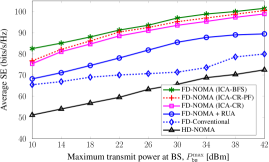
(a) Average SE versus $P_{\mathtt{bs}}^{\max}$ for different schemes.

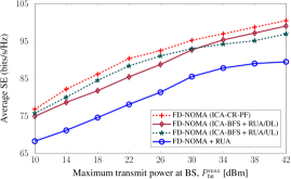
(b) Average SE versus $P_{\mathtt{bs}}^{\max}$ with RUA for DL and/or UL transmission.

Figure 3: Average SE versus the BS transmit power, $P_{\mathtt{bs}}^{\max}$.

 

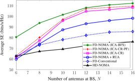
(a) Average SE versus $N$.

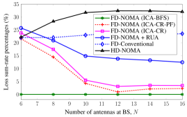
(b) Percentage of loss-SE versus $N$.

Figure 4: The change of average SE versus the number of antennas at the BS, $N$.

Fig. 3 depicts the average SEs versus the maximum transmit power at the BS for different resource allocation schemes. As expected in Fig. 3(a), the ICA-BFS based algorithm provides the best SE due to finding the best UA for the FD-NOMA. However, we recall that it requires extremely high complexity, and thus, only plays as a benchmark. In addition, the ICA-CR-PF based algorithm tends to outperform the ICA-CR based algorithm as it aims at finding a high-performance UA solution. On the other hand, it can be seen that both ICA-CR based algorithms deviate only 1$\%\sim 2\%$ from the optimal SE, meaning that performances are very good but with much less complexity compared to the ICA-BFS based algorithm. Unsurprisingly, our proposed FD-NOMA schemes outperform the conventional ones. Fig. 3(b) further demonstrates the role of UA in DL and UL transmissions. Upon utilizing the BFS method, two other cases are considered: ($i$) “ICA-BFS + RUA/DL”: We use the ICA-BFS for optimizing UL users’ decoding order and random DL user pairing, and $(ii)$ “ICA-BFS + RUA/UL”: The ICA-BFS is used for random UL users’ decoding order and optimizing DL user pairing. As shown in Fig. 3(b), the optimization of UA in either DL or UL transmission enjoys a significant improvement of the SE as compared to FD-NOMA with RUA. The results also show that the UA in both DL and UL transmissions has significant influence on the performance. Although performances of “ICA-BFS + RUA/DL” and “ICA-BFS + RUA/UL” are comparable, they are distinguished from each other when $P_{\mathtt{bs}}^{\max}$ varies. It is clear that increasing $P_{\mathtt{bs}}^{\max}$ merely assists the DL transmission. The performance of “ICA-BFS + RUA/DL” is inferior when $P_{\mathtt{bs}}^{\max}<30$ dBm, since the total SE is mainly determined by the DL transmission. Increasing $P_{\mathtt{bs}}^{\max}$ brings much benefit to the optimization of UL users’ decoding order as the performance of “ICA-BFS + RUA/UL” is lower than that of “ICA-BFS + RUA/DL” when $P_{\mathtt{bs}}^{\max}>32$ dBm. These results again confirm the important roles of user association in FD-NOMA systems.

In Fig. 4(a), we plot the average SE versus the number of antennas at the BS, $N\in[6,16]$. First, for small $N$ (i.e., $N\leq 6$), ICA-CR based schemes provide the same performance (even worse) compared to the conventional ones. This is because the BS has a limited degrees-of-freedom to exploit multiuser diversity, which may result in a severe network interference situation in FD-NOMA based schemes. In this case, the use of UA in ICA-CR based schemes becomes less efficient. However, when $N$ increases, the SE gains of the proposed FD-NOMA schemes over the other ones are remarkable. The reason is that the BS in FD-NOMA has sufficient degrees-of-freedom to select the best UA solutions, without causing much interference to the other users. To further comprehend the benefit of using UA, Fig. 4(b) shows the percentages of loss-SE in comparison with the optimal performance obtained by the ICA-BFS.

Fig. 6 shows the cumulative distribution function (CDF) of the FD-based schemes as a function of the QoS requirement, $\bar{R}$. The HD-NOMA scheme is omitted here since its DL and UL transmissions are separately executed. It can be seen that the probabilities of feasibility of all the considered schemes are smaller when $\bar{R}$ is higher. As expected, FD-NOMA schemes can maintain much rate fairness among all the DL and UL users as compared to the FD-Conventional scheme. In addition, FD-NOMA schemes using the ICA-CR and ICA-CR-PF based algorithms offset about 0.5 bits/s/Hz and 2 bits/s/Hz of the rate threshold more than the scheme of FD-NOMA with RUA, respectively, in about 50$\%$ of the simulated trials. It further confirms that the joint optimization of UA might help satisfy higher QoS levels for the FD-NOMA schemes. Clearly, the ICA-CR-PF based algorithm assisted by the PF outperforms the ICA-CR one. The reason is that the former can quickly find the satisfactory solution of DL user pairing and UL users’ decoding, at which the QoS constraints are satisfied even under unexpected channel conditions. The CDFs w.r.t. the rate threshold validate the advantage of UA, and reflect the characteristics of the proposed algorithms.

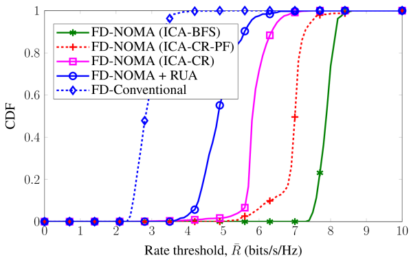
Figure 5: Cumulative distribution function versus the rate threshold.

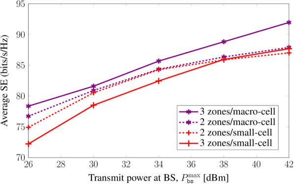
Figure 6: Average SE versus $P_{\mathtt{bs}}^{\max}$ for different numbers of zones/clusters using the ICA-CR-PF based algorithm.

As mentioned previously in Section II-C, we now provide simulation results for two- and three-zone in scenarios of small- (100-meter radius) and macro-cells (500-meter radius), as illustrated in Fig. 6. The number of UL users is the same as before. We place 12 DL users to fairly compare the system performance of 2- and 3-zone DL transmissions, where NOMA is applied to 6 clusters (2 users in each) and 4 clusters (3 users in each), respectively. We use the ICA-CR-PF based algorithm for this investigation since it provides a good performance, with low complexity per iteration and fast convergence rate. In general, DL NOMA used for the macro-cell offers more efficient than that in small-cell, since DL users in the same cluster in macro-cell have significantly different channel gains. In addition, the dense multi-user interference in the small-cell deteriorates the system performance. Numerically, it is observed that the 3-zone NOMA provides the best SE for the macro-cell. However, it tends to perform the worst in the small-cell. This is because FD-NOMA systems for the small-cell scenario suffer from both the similar channel conditions and mutually strong interference. These results corroborate that in a small-cell scenario, the NOMA using 2-zone model outperforms that using the 3-zone one. In other words, a number of DL clusters should be properly chosen depending on the realistic scenarios.

VI-C Effects of SI, CCI and Rate Threshold

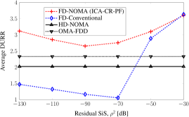
(a) Average DURR versus residual SiS, $\rho^{2}$.

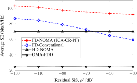
(b) Average SE versus residual SiS, $\rho^{2}$.

Figure 7: The effects of SI on DURR and SE.

In Fig. 7, we show the effects of SI on the system performance by varying $\rho^{2}$ from $-130$ dB to $-30$ dB. For this purpose, we also consider the orthogonal multiple access with frequency division duplexing (OMA-FDD) scheme. In particular, the entire system bandwidth is partitioned into $(L+M)$ orthogonal sub-bandwidths, and each sub-bandwidth is allocated to at most one user to avoid interference. Fig. 7(a) plots the DL-to-UL rate ratio (DURR) with respect to $\rho^{2}$. As expected, DURRs of HD-NOMA and OMA-FDD are unchanged with varying $\rho^{2}$ since there is no SI on these schemes. We also observe that for FD schemes, DURRs first decrease and then increase when $\rho^{2}$ increases. This reveals an interesting result which can be explained as follows. For very small $\rho^{2}$, BS pays more attention to DL users to maximize the total SE since the effect of SI is negligible. For moderate $\rho^{2}$, BS aims to balance the performance between DL and UL by scaling down its transmit power to mitigate the effect of SI. When $\rho^{2}$ becomes more stringent, BS sacrifices the performance of UL by scaling up its transmit power to boost that of DL, as long as the total SE is maximized. Such phenomena also confirm the performance degradation of FD schemes with $\rho^{2}$ in Fig. 7(b). Interestingly, the SE of the proposed FD-NOMA is quite robust to the SI and always outperforms the HD-NOMA for a given range of $\rho^{2}$, which further confirms the benefit of optimizing UL users’ decoding order. Moreover, the proposed FD-NOMA provides much better SE than the OMA-FDD at $\rho^{2}=-30$ dB due to its potential to improve both SE and edge throughput.

To evaluate the effect of CCI on system performance, we examine a simulation setup as illustrated in Fig. 8(a), in which the centered-BS equipped with 4 antennas serves 4 DL users with fixed locations and 2 UL users with fixed distances to the BS simultaneously moving along with a rotation angle, $\varphi_{\mathtt{r}}$. The group of DL users on the right-hand side (RHS group) includes $\mathtt{U}_{11}^{\mathtt{d}}$ and $\mathtt{U}_{21}^{\mathtt{d}}$, while the group of DL users on the left-hand side (LHS group) is formed by $\mathtt{U}_{12}^{\mathtt{d}}$ and $\mathtt{U}_{22}^{\mathtt{d}}$. To better illustrate the effect of CCI, we define the sum SE of DL users in the RHS and LHS groups as $R_{11+21}^{\mathtt{d}}$ and $R_{12+22}^{\mathtt{d}}$, respectively. Fig. 8(b) depicts $R_{11+21}^{\mathtt{d}}$ and its ratio over $R_{11+21}^{\mathtt{d}}+R_{12+22}^{\mathtt{d}}$. As expected, $R_{11+21}^{\mathtt{d}}$ increases when UL users move far away from DL users in the RHS group, i.e., $\varphi_{\mathtt{r}}\in\{0,\pi/4,\pi/2\}$. When $\varphi_{\mathtt{r}}\in\{3\pi/4,\pi\}$, $R_{11+21}^{\mathtt{d}}$ decreases due to the strong effect of CCI on DL users in the LHS group. The reason is that the BS needs to allocate more power to DL users in the LHS group to combat the strong CCI, leading to a lower power for DL users in the RHS group. The medium ratio of $R_{11+21}^{\mathtt{d}}$ to $R_{11+21}^{\mathtt{d}}+R_{12+22}^{\mathtt{d}}$ w.r.t. $\varphi_{\mathtt{r}}$ on the right y-axis implies that the proposed FD-NOMA offers uniform service to DL users. Accordingly, it is expected to outperform other FD schemes in maximizing the total SE, as seen from results on the left y-axis. Fig. 8(c) further examines $R_{11+21}^{\mathtt{d}}$ versus $\varphi_{\mathtt{r}}$ with different values of $\bar{R}\in\{0,1,2,4\}$. Clearly, $R_{11+21}^{\mathtt{d}}$ deteriorates with $\bar{R}$, leading to the infeasibility of the proposed algorithm under the strong effect of CCI and higher required rate, i.e., $\varphi_{\mathtt{r}}\in\{0,\pi\}$ and $\bar{R}=4$ bits/s/Hz.

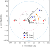
(a) Simulation setup considered in Figs. 8(b) and 8(c), with $r_{1}=25$m, $r_{2}=75$m, $\Delta r=1$m, $N=4$, $K=2$ and $L=2$.

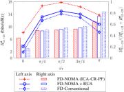
(b) $R_{11+21}^{\mathtt{d}}$ and its ratio over $R_{11+21}^{\mathtt{d}}+R_{12+22}^{\mathtt{d}}$.

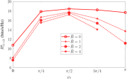
(c) $R_{11+21}^{\mathtt{d}}$ with different rate thresholds using FD-NOMA (ICA-CRP-PF), $\bar{R}$.

Figure 8: The effects of CCI and rate threshold, with the simulation setup in Fig. 8(a).

VI-D Convergence Behavior

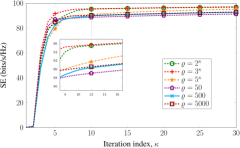
(a) Convergence speed of ICA-CR-PF with different values of $\varrho$.

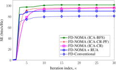
(b) Convergence speed for different schemes.

Figure 9: Typical convergence behavior of the proposed algorithms with one random channel realization.

In Fig. 9, we explore the convergent properties of the proposed algorithms. First, the effect of the penalty parameter $\varrho$ (i.e., step 4 of Alg. 2) on the convergence behavior and performance of the ICA-CR-PF algorithm is investigated in Fig. 9(a). Herein, $\varrho$ is numerically examined in two cases: given values as $\varrho\in\{50,500,5000\}$ and adaptive values per iteration as $\varrho=a^{\kappa}$, with $a\in\{2,3,5\}$. In the first case, the given values of $\varrho$, which are larger than $\mfrac{1}{(L+2K)\epsilon(1-\epsilon)}\ln\bigl{(}\mfrac{P_{\mathtt{bs}}^{\max}}{B.\sigma^{2}}\bigr{)}$ (i.e., eq. (C.5)) are sufficiently estimated according to $\epsilon=\{10^{-1},10^{-2},10^{-3}\}$, respectively. It is seen that for $\varrho=\{500,5000\}$, the SEs at the 10-th iteration reach more than 90% of that at the 50-th iteration. Although the proposed ICA-CR-PF algorithm with $\varrho=50$ provides the same performance ratio after the 5-th iteration, the achievable SE is worse than that for $\varrho=\{500,5000\}$. In the second case, an increase in $\varrho$ per iteration makes the algorithm converge faster. The results clearly show that the ICA-CR-PF algorithm with $\varrho=3^{\kappa}$ outperforms the others. Fig. 9(b) illustrates the convergence rates of five FD schemes, in which the ICA-CR-PF algorithm uses $\varrho=3^{\kappa}$. We exclude the convergence behavior of the HD-NOMA scheme, since it separates the optimization for DL and UL transmissions. As seen, the proposed algorithms provide better performance compared to the others. Fig. 9(b) also shows that, compared to the ICA-CR based algorithm, the ICA-CR-PF based algorithm converges much faster. This can be attributed to the fact that the absence of the PF in the ICA-CR based algorithm may take more iterations to stabilize.

Finally, we provide further insight of selection of $\varrho$ in the ICA-CR-PF based algorithm, as illustrated in Fig. 10. As earlier shown, $\varrho=a^{\kappa}$ provides faster convergence. However, the best value of $a$ mainly depends on the specific setting. Therefore, the ICA-CR-PF based algorithm combined with the binary search is used to find $a$ just once. To evaluate the effectiveness of $a$, we define the convergence measurements as $\mathbf{u}\triangleq\mathrm{vec}\bigl{(}\bigl{[}[\alpha_{kj}^{2}-\alpha_{kj}]_{k,j\in\mathcal{K}}\;[\beta_{\ell m}^{2}-\beta_{\ell m}]_{\ell,m\in\mathcal{L}}\bigr{]}\bigr{)}$ and $\mathbf{\hat{f}}_{p}\triangleq 0.1\mathrm{vec}\bigl{(}\bigl{[}[f_{p}(\alpha_{kj})]_{k,j\in\mathcal{K}}\;[f_{p}(\beta_{\ell m})]_{\ell,m\in\mathcal{L}}\bigr{]}\bigr{)}$, where $\mathrm{vec}(\mathbf{X})$ represents the vectorization of the matrix $\mathbf{X}$. Remark 3 indicates that $a$ is selected such that $\varrho$ should not be too large, to satisfy the condition in (C.5). Numerically, the convergence rate of $\|\mathbf{u}\|_{\infty}$ and $\|\mathbf{\hat{f}}_{p}\|_{\infty}$ is the best when $a$ is large enough, and however, it becomes worse when $a$ further increases. In implementation, the binary search is used for finding $a\in[2,5]$, and for each value of $a$, the ICA-CR-PF based algorithm investigates the values of $\|\mathbf{u}\|_{\infty}$ and $\|\mathbf{\hat{f}}_{p}\|_{\infty}$ so that the smallest value of $a$ providing the lowest convergence rates of $\|\mathbf{u}\|_{\infty}$ and $\|\mathbf{\hat{f}}_{p}\|_{\infty}$ is selected. For example, Fig. 10 depicts the values of $\|\mathbf{u}\|_{\infty}$ and $\|\mathbf{\hat{f}}_{p}\|_{\infty}$ (left y-axis) and penalty parameter $\varrho$ (right y-axis) versus the iteration index $\kappa$ (common x-axis) in the cases of $a=\{2,3\}$. For the above setting, $a=3$ in Fig. 10(b) is a better choice as it provides the lower convergence rates of $\|\mathbf{u}\|_{\infty}$ and $\|\mathbf{\hat{f}}_{p}\|_{\infty}$. We have also numerically observed that when $a>3$, the quick increase in $\varrho$ per iteration contradicts Remark 3. Therefore, the smallest value of $a$ needs to be found within $[2,3]$. Whenever the sufficient value of $a$ is found, the ICA-CR-PF based algorithm can operate under different channel conditions. Remarkably, the convergence behaviors of the UA variables are almost same at the beginning of setting. It can be seen that the values of $\boldsymbol{\alpha}$ and $\boldsymbol{\beta}$ are close to binary at the 9-th iteration. Thus, without loss of optimality, the binary variables can be fixed as in (32) when $\|\mathbf{u}\|_{\infty}$ satisfies a given error tolerance, and then, the ICA-CR-PF based algorithm continuously solves problem (36) for power control as equivalent to a subproblem (48).

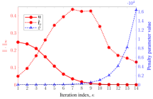
(a) $\varrho=2^{\kappa}$

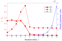
(b) $\varrho=3^{\kappa}$

Figure 10: Convergence rate of UA variables and PF values with $\varrho=a^{\kappa}$, for $a=\{2,3\}$.

VII Conclusion

In this paper, joint power control and user association problem has been proposed to maximize the total SE of a cellular FD-NOMA system. We have employed a tensor model for DL users and a permutation matrix for UL users to formulate the problem of user association, which significantly reduce the number of association variables. By presenting novel methods to approximate the formulated non-convex problem, we have developed two iterative algorithms with low computational complexity. In the first method, the binary variables are relaxed to be continuous and an iterative algorithm based on the ICA framework has been proposed to solve the resulting non-convex CR problem. In the second method, the uncertainties of binary variables are further penalized without causing additional complexity as it aims at finding a high-performance UA solution. Our extensive numerical results suggest that the second approach is more effective in terms of the achievable SE and convergence speed. In addition, by the brute-force search algorithm, we have transformed the original problem into subproblems under a given UA based on which the ICA framework has been customized to find an optimal solution. Our proposed iterative algorithms improve achievable SE at each iteration and converge eventually, and are also superior to other known algorithms. We have also concluded that an appropriate number of zones/clusters with more distinct channel conditions is of important to achieve remarkable gains in FD-NOMA systems. The robustness of the proposed method against the significant effects of SI and CCI is also revealed.

Appendix A Proof of Theorem 1

Let $\mathbf{C}_{0}$ be the unitary matrix representing the clustering indices. It is obvious that $\mathbf{C}_{i},\;i\in\mathcal{Z},$ is the change-of-basis matrix of zone $i$, with respect to the basis $\mathbf{C}_{0}$. Therefore, $\bigl{[}\mathbf{C}_{i}\bigr{]}_{kj},\;k,j\in\mathcal{K}$, with $[\mathbf{X}]_{a,b}$ denoting the element at the $a$-th row and the $b$-th column of matrix $\mathbf{X}$, indicates whether the $j$-th DL user in zone $i$ belongs to the $k$-th cluster. From Definition 2, the matrix of DL user associations between users in zone $1$ and clusters is equivalent to the change-of-basis matrix $\mathbf{C}_{1}$, i.e., $\mathbf{C}_{1}=\mathbf{C}_{0}=\mathbf{I}_{K}$. As a result, a user association matrix $\mathbf{T}^{1i}$ is equivalent to the change-of-basis matrix $\mathbf{C}_{i}$ w.r.t. the basis $\mathbf{C}_{0}$. From the transformation law of tensor, the user association matrix $\mathbf{T}^{iz},\;(i,z)\in\{\mathcal{Z}\times\mathcal{Z}\}$ is calculated by

$$\mathbf{T}^{iz}=\bigl{(}\mathbf{T}^{1i}\bigr{)}^{-1}\mathbf{C}_{1}\mathbf{C}_{z}=\mathbf{C}_{i}^{-1}\mathbf{C}_{z}.$$ (A.1)

Based on Definition 1, it is realized that each DL user in a certain zone is assigned to exactly one cluster, and two arbitrary DL users in each cluster come from two different zones. Therefore, the matrix $\mathbf{C}_{i},\;i\in\mathcal{Z}$, satisfies the following conditions:

$$\sum\nolimits_{k\in\mathcal{K}}\bigl{[}\mathbf{C}_{i}\bigr{]}_{kj}=1\ \text{and}\ \sum\nolimits_{j\in\mathcal{K}}\bigl{[}\mathbf{C}_{i}\bigr{]}_{kj}=1.$$ (A.2)

Accordingly, $\mathbf{C}_{i}$ characterized as a permutation matrix, satisfies the property that $\mathbf{C}_{i}^{-1}=\mathbf{C}_{i}^{T}$. Equation (1) is then obtained by substituting $\mathbf{C}_{i}^{-1}=\mathbf{C}_{i}^{T}$ into (A.1).

Appendix B Proof of Lemma 1

By imposing an SOC constraint $y^{2}\leq z,\;z>0$, the function $h(x,y)$ is upper bounded by

$$h(x,y)\leq xz:=\tilde{h}(x,z).$$ (B.1)

Due to the concavity of function $\sqrt{uv}$, we make use of the following inequality [34, 19]:

$$\sqrt{uv}\leq\mfrac{\sqrt{v^{(\kappa)}}}{2\sqrt{u^{(\kappa)}}}u+\mfrac{\sqrt{u^{(\kappa)}}}{2\sqrt{v^{(\kappa)}}}v,$$ (B.2)

for any $u,v,u^{(\kappa)},v^{(\kappa)}>0$, where $u^{(\kappa)}$ and $v^{(\kappa)}$ are the known neighborhoods of $u$ and $v$, respectively. By letting $x=\sqrt{u},\;z=\sqrt{v}$, and substituting (B.2) into (B.1), we arrive at (16).

Appendix C Proof of Theorem 2

Firstly, we can treat constraint (33c) as $\alpha_{n}(\alpha_{n}-1)=0,\;\forall n\in\mathcal{N}$, which is equivalent to

$$\alpha_{n}(\alpha_{n}-1)\geq 0,$$ (C.1a)

$$\alpha_{n}(\alpha_{n}-1)\leq 0.$$ (C.1b)

For the non-convex constraint (C.1a), we apply the relaxation approach to release (C.1a), where $\alpha_{n}$ is constrained by a box $[0,1]$, i.e., $\alpha_{n}^{2}\leq\alpha_{n}$ for $0\leq\alpha_{n}\leq 1$. Inspired from [22], we then introduce an additional PF, denoted by $f_{p}(\alpha_{n})$, satisfying:

$$f_{p}(\alpha_{n})=\left\{\begin{aligned} -\infty,&\quad\text{ if }0<\alpha_{n}<1,\\ 0,&\quad\text{ if }\alpha_{n}\in\{0,1\}.\end{aligned}\right.$$ (C.2)

This indicates that the objective value for the maximization problem becomes $-\infty$ when constraint (33c) is violated. Numerically, the objective value is corrupted by a large penalty parameter, such that it becomes smaller than an estimated optimal value $\hat{f}_{0}(\mathbf{x},\boldsymbol{\alpha})$ when $\alpha_{n}$ is not binary. By exploiting the convexity of (C.1b), the PF can be constructed as $f_{p}(\alpha_{n})\triangleq\varrho_{n}(\alpha_{n}^{2}-\alpha_{n}),\;\forall n\in\mathcal{N}$, to meet the condition in (C.2). Herein, $\alpha_{n}^{2}-\alpha_{n}\leq 0$ provides a well-defined set mapping into the codomain of $f_{p}$ in (C.2) for $\alpha_{n}\in[0,1]$, while $\varrho_{n}>0$ is selected to be large enough such that the optimality of (33) holds. By this way, the relaxation problem (34) is provided.

Secondly, we need to demonstrate how $\varrho_{n}>0$ is found to ensure the optimal solution of (33) by solving the relaxation problem with PF in (34). Let $\mathcal{F}=\mathcal{X}\times\{0,1\}^{N_{\alpha}\times 1}$ and $\mathcal{F}_{R}=\mathcal{X}\times[0,1]^{N_{\alpha}\times 1}$ be the feasible regions of (33) and (34), respectively, and suppose that $\mathbf{y}^{*}\in\mathcal{F}$ and $\mathbf{y}_{r}^{*}\in\mathcal{F}_{R}$ are their optimal solutions. If $\mathbf{y}^{*}\in\mathcal{F}\subset\mathcal{F}_{R}$, $\mathbf{y}^{*}\in\mathcal{F}_{R}$ provides a lower bound of $f_{0}(\mathbf{y}_{r}^{*})$, i.e., $f_{0}(\mathbf{y}^{*})\leq f_{0}(\mathbf{y}_{r}^{*})$. To find $\varrho_{n}$, we consider a part of feasible region of the relaxation problem as $\bar{\mathcal{F}}\triangleq\{\mathbf{y}_{r}=(\mathbf{x},\boldsymbol{\alpha})\in\mathcal{F}_{R}\backslash\mathcal{F}\;|\epsilon\leq\alpha_{n}\leq 1-\epsilon,\forall n\in\mathcal{N}\}$, with $\epsilon\in(0,1)$ being an arbitrarily small number such that $\mathcal{F}\cong\mathcal{F}_{R}\backslash\bar{\mathcal{F}}$. If any $\mathbf{\hat{y}}^{*}\in\mathcal{F}_{R}\backslash\bar{\mathcal{F}}$, the optimal solution of (34) is close to that of (33), i.e., $\mathbf{\hat{y}}^{*}\rightarrow\mathbf{y}^{*}$. The penalty parameter $\varrho_{n}>0$ must be selected to satisfy

$$\underset{\mathbf{\bar{y}}^{*}\in\bar{\mathcal{F}}}{\sup}\bigl{(}f_{0}(\mathbf{\bar{y}}^{*})+\sum\nolimits_{n\in\mathcal{N}}f_{p}(\alpha_{n})\bigr{)}=\sum\nolimits_{n\in\mathcal{N}}f_{p}(\alpha_{n})+\underset{\mathbf{\bar{y}}^{*}\in\bar{\mathcal{F}}}{\sup}\;f_{0}(\mathbf{\bar{y}}^{*})\leq\underset{\mathbf{y}^{*}\in\mathcal{F}}{\inf}\;f_{0}(\mathbf{y}^{*}).$$ (C.3)

On the other hand, it is clear that $\alpha_{n}(\alpha_{n}-1)\leq\epsilon(\epsilon-1)$ due to $\alpha_{n}\in[\epsilon,1-\epsilon]$ and $\bar{\mathcal{F}}\subseteq\mathcal{F}_{R}$. Therefore, $\sum_{n\in\mathcal{N}}f_{p}(\alpha_{n})$ and $\underset{\mathbf{\bar{y}}^{*}\in\bar{\mathcal{F}}}{\sup}\;f_{0}(\mathbf{\bar{y}}^{*})$ are respectively upper bounded as

$$\sum\nolimits_{n\in\mathcal{N}}f_{p}(\alpha_{n}) \leq\sum\nolimits_{n\in\mathcal{N}}\varrho\epsilon(\epsilon-1)=N_{\alpha}\varrho\epsilon(\epsilon-1)<0,$$ (C.4a)

$$\underset{\mathbf{\bar{y}}^{*}\in\bar{\mathcal{F}}}{\sup}\;f_{0}(\mathbf{\bar{y}}^{*}) \leq\underset{\mathbf{y}_{r}^{*}\in\mathcal{F}_{R}}{\sup}\;f_{0}(\mathbf{y}_{r}^{*}),$$ (C.4b)

where $\varrho\triangleq\max\{\varrho_{n}\}_{n\in\mathcal{N}}$. The inequality (C.3) strongly holds with (C.4), and then we obtain

$$\varrho\geq\mfrac{1}{N_{\alpha}\epsilon(\epsilon-1)}\Bigl{(}\underset{\mathbf{y}^{*}\in\mathcal{F}}{\inf}\;f_{0}(\mathbf{y}^{*})-\underset{\mathbf{y}_{r}^{*}\in\mathcal{F}_{R}}{\sup}\;f_{0}(\mathbf{y}_{r}^{*})\Bigr{)}.$$ (C.5)

Since the function $f_{0}$ is closed and bounded on $\mathcal{F}$, it is also closed and bounded on $\mathcal{F}_{R}$ for $\boldsymbol{\alpha}\in[0,1]$. Moreover, $\mathcal{F}\subset\mathcal{F}_{R}$ indicates that $\underset{\mathbf{y}_{r}^{*}\in\mathcal{F}_{R}}{\inf}\;f_{0}(\mathbf{y}_{r}^{*})\leq\underset{\mathbf{y}^{*}\in\mathcal{F}}{\inf}\;f_{0}(\mathbf{y}^{*})<\underset{\mathbf{y}^{*}\in\mathcal{F}}{\sup}\;f_{0}(\mathbf{y}^{*})\leq\underset{\mathbf{y}_{r}^{*}\in\mathcal{F}_{R}}{\sup}\;f_{0}(\mathbf{y}_{r}^{*})$, resulting in the positive value for the RHS of (C.5). The inequality (C.5) also means that there exists $\varrho>0$ so that the penalty parameter satisfies the condition (C.3). Note that the smaller value of $\epsilon$ in (C.5) results in a larger value of its RHS. Therefore, $\varrho$ needs to be selected such that it is adapted to $\epsilon$.

Finally, we consider the property of the feasible set. Assuming $\mathcal{X}$ is a compact convex set. In problem (34), we have $\alpha_{n}\in\mathcal{I}\triangleq[0,1],\;\forall n\in\mathcal{N}$. Since $\mathcal{I}$ is a closed interval, $\mathcal{I}$ is compact [42]. Considering $\delta=\theta\alpha+(1-\theta)\beta$ for $\forall\alpha,\beta\in\mathcal{I},\;0\leq\theta\leq 1$, we have $0\leq\theta\alpha\leq\theta$ and $0\leq(1-\theta)\beta\leq(1-\theta)$. This means that $0\leq\delta\leq 1$, or $\delta\in\mathcal{I}$, leading to the fact that $\mathcal{I}$ is convex. Therefore, the feasible set of (34) is $\mathcal{X}\times\mathcal{I}$, which is a compact convex set. Thus, the proof is completed.

References

- [1] J. Andrews, S. Buzzi, W. Choi, S. Hanly, A. Lozano, A. Soong, and J. Zhang, “What will 5G be?” IEEE J. Select. Area Commun., vol. 32, no. 6, pp. 1065–1082, June 2014.
- [2] A. Yadav and O. A. Dobre, “All technologies work together for good: A glance at future mobile networks,” IEEE Wireless Commun., vol. 25, no. 4, pp. 10–16, Aug. 2018.
- [3] Z. Ding, Y. Liu, J. Choi, Q. Sun, M. Elkashlan, C. L. I, and H. V. Poor, “Application of non-orthogonal multiple access in LTE and 5G networks,” IEEE Commun. Mag., vol. 55, no. 2, pp. 185–191, Feb. 2017.
- [4] Y. Liu, Z. Qin, M. Elkashlan, Z. Ding, A. Nallanathan, and L. Hanzo, “Nonorthogonal multiple access for 5G and beyond,” Proc. of the IEEE, vol. 105, no. 12, pp. 2347–2381, Dec. 2017.
- [5] S. M. R. Islam, N. Avazov, O. A. Dobre, and K.-S. Kwak, “Power-domain non-orthogonal multiple access (NOMA) in 5G systems: Potentials and challenges,” IEEE Commun. Surveys Tutor., vol. 19, no. 2, pp. 721–742, Second quarter 2017.
- [6] S. M. R. Islam, M. Zeng, O. A. Dobre, and K. Kwak, “Resource allocation for downlink NOMA systems: Key techniques and open issues,” IEEE Wireless Commun., vol. 25, no. 2, pp. 40–47, Apr. 2018.
- [7] Z. Ding, X. Lei, G. K. Karagiannidis, R. Schober, J. Yuan, and V. K. Bhargava, “A survey on non-orthogonal multiple access for 5G networks: Research challenges and future trends,” IEEE J. Select. Areas Commun., vol. 35, no. 10, pp. 2181–2195, Oct. 2017.
- [8] Z. Ding, P. Fan, and H. V. Poor, “Impact of user pairing on 5G nonorthogonal multiple-access downlink transmissions,” IEEE Trans. Veh. Tech., vol. 65, no. 8, pp. 6010–6023, Aug. 2016.
- [9] C. Chen, W. Cai, X. Cheng, L. Yang, and Y. Jin, “Low complexity beamforming and user selection schemes for 5G MIMO-NOMA systems,” IEEE J. Select. Areas Commun., vol. 35, no. 12, pp. 2708–2722, Dec. 2017.
- [10] V. W. Wong, R. Schober, D. W. K. Ng, and L.-C. Wang, Key Technologies for 5G Wireless Systems. Cambridge, MA, USA: Cambridge Univ. Press, 2017.
- [11] A. Yadav, G. I. Tsiropoulos, and O. A. Dobre, “Full-duplex communications: Performance in ultradense mm-wave small-cell wireless networks,” IEEE Veh. Technol. Mag., vol. 13, no. 2, pp. 40–47, June 2018.
- [12] D. Bharadia, E. McMilin, and S. Katti, “Full duplex radios,” in Proc. ACM SIGCOMM Computer Commun. Review, vol. 43, no. 4, 2013, pp. 375–386.
- [13] A. Sabharwal, P. Schniter, D. Guo, D. W. Bliss, S. Rangarajan, and R. Wichman, “In-band full-duplex wireless: Challenges and opportunities,” IEEE J. Select. Areas Commun., vol. 32, no. 9, pp. 1637–1652, Feb. 2014.
- [14] D. Bharadia and S. Katti, “Full duplex MIMO radios,” in Proc. 11th USENIX Symp. Netw. Syst. Design Implement. (NSDI), Seattle, WA, USA, 2014, pp. 369–372.
- [15] D. Nguyen, L.-N. Tran, P. Pirinen, and M. Latva-aho, “On the spectral efficiency of full-duplex small cell wireless systems,” IEEE Trans. Wireless Commun., vol. 13, no. 9, pp. 4896–4910, Sept. 2014.
- [16] P. Aquilina, A. C. Cirik, and T. Ratnarajah, “Weighted sum rate maximization in full-duplex multi-user multi-cell MIMO networks,” IEEE Trans. Commun., vol. 65, no. 4, pp. 1590–1608, Apr. 2017.
- [17] V.-D. Nguyen, H. V. Nguyen, C. T. Nguyen, and O.-S. Shin, “Spectral efficiency of full-duplex multiuser system: Beamforming design, user grouping, and time allocation,” IEEE Access, vol. 5, pp. 5785–5797, Mar. 2017.
- [18] A. Yadav, O. A. Dobre, and N. Ansari, “Energy and traffic aware full duplex communications for 5G systems,” IEEE Access, vol. 5, pp. 11 278–11 290, May 2017.
- [19] V.-D. Nguyen, H. V. Nguyen, O. A. Dobre, and O.-S. Shin, “A new design paradigm for secure full-duplex multiuser systems,” IEEE J. Select. Areas Commun., vol. 36, no. 7, pp. 1480–1498, July 2018.
- [20] H. H. M. Tam, H. D. Tuan, and D. T. Ngo, “Successive convex quadratic programming for quality-of-service management in full-duplex MU-MIMO multicell networks,” IEEE Trans. Commun., vol. 64, no. 6, pp. 2340–2353, June 2016.
- [21] H. V. Nguyen, V.-D. Nguyen, O. A. Dobre, Y. Wu, and O.-S. Shin, “Joint antenna array mode selection and user assignment for full-duplex MU-MISO systems,” IEEE Trans. Wireless Commun., vol. 18, no. 6, pp. 2946–2963, June 2019.
- [22] Y. Sun, D. W. K. Ng, Z. Ding, and R. Schober, “Optimal joint power and subcarrier allocation for full-duplex multicarrier non-orthogonal multiple access systems,” IEEE Trans. Commun., vol. 65, no. 3, pp. 1077–1091, Mar. 2017.
- [23] Z. Ding, P. Fan, and H. V. Poor, “On the coexistence between full-duplex and NOMA,” IEEE Wireless Commun. Lett., vol. 7, no. 5, pp. 692–695, Oct. 2018.
- [24] Y. Sun, D. W. K. Ng, J. Zhu, and R. Schober, “Robust and secure resource allocation for full-duplex MISO multicarrier NOMA systems,” IEEE Trans. Commun., vol. 66, no. 9, pp. 4119–4137, Sept. 2018.
- [25] H. V. Nguyen, V.-D. Nguyen, and O.-S. Shin, “Joint NOMA beamforming and user scheduling for sum rate maximization in a full-duplex system,” in Proc. Inter. Conf. Inform. Commun. Technol. Converg. (ICTC), Oct. 2017, pp. 731–733.
- [26] B. K. Chalise, H. A. Suraweera, G. Zheng, and G. K. Karagiannidis, “Beamforming optimization for full-duplex wireless-powered MIMO systems,” IEEE Trans. Commun., vol. 65, no. 9, pp. 3750–3764, Sept. 2017.
- [27] J. Choi, “Minimum power multicast beamforming with superposition coding for multiresolution broadcast and application to NOMA systems,” IEEE Trans. Commun., vol. 63, no. 3, pp. 791–800, Mar. 2015.
- [28] Z. Chen, Z. Ding, X. Dai, and G. K. Karagiannidis, “On the application of quasi-degradation to MISO-NOMA downlink,” IEEE Trans. Signal Process., vol. 64, no. 23, pp. 6174–6189, Dec. 2016.
- [29] Z. Chen, Z. Ding, and X. Dai, “Beamforming for combating inter-cluster and intra-cluster interference in hybrid NOMA systems,” IEEE Access, vol. 4, pp. 4452–4463, 2016.
- [30] M. F. Hanif, Z. Ding, T. Ratnarajah, and G. K. Karagiannidis, “A minorization-maximization method for optimizing sum rate in the downlink of non-orthogonal multiple access systems,” IEEE Trans. Signal Process., vol. 64, no. 1, pp. 76–88, Jan. 2016.
- [31] Z. Ding, R. Schober, and H. V. Poor, “A general MIMO framework for NOMA downlink and uplink transmission based on signal alignment,” IEEE Trans. Wireless Commun., vol. 15, no. 6, pp. 4483–4454, June 2016.
- [32] V.-D. Nguyen, H. D. Tuan, T. Q. Duong, H. V. Poor, and O.-S. Shin, “Precoder design for signal superposition in MIMO-NOMA multicell networks,” IEEE J. Select. Areas Commun., vol. 35, no. 12, pp. 2681–2695, Dec. 2017.
- [33] B. R. Marks and G. P. Wright, “A general inner approximation algorithm for nonconvex mathematical programs,” Operations Research, vol. 26, no. 4, pp. 681–683, July-Aug. 1978.
- [34] A. Beck, A. Ben-Tal, and L. Tetruashvili, “A sequential parametric convex approximation method with applications to nonconvex truss topology design problems,” J. Global Optim., vol. 47, no. 1, pp. 29–51, May 2010.
- [35] D. Tse and P. Viswanath, Fundamentals of Wireless Communication. Cambridge Univ. Press, UK, 2005.
- [36] S. Boyd and L. Vandenberghe, Convex Optimization. Cambridge Univ. Press, UK, 2007.
- [37] V.-D. Nguyen, T. Q. Duong, H. D. Tuan, O.-S. Shin, and H. V. Poor, “Spectral and energy efficiencies in full-duplex wireless information and power transfer,” IEEE Trans. Commun., vol. 65, no. 5, pp. 2220–2233, May 2017.
- [38] K. Bestuzheva and H. Hijazi, “Invex optimization revisited,” July 2017. [Online]. Available: https://arxiv.org/abs/1707.01554v1
- [39] D. Peaucelle, D. Henrion, Y. Labit, and K. Taitz, “User’s guide for SeDuMi interface 1.04,” in LAAS-CNRS, Toulouse, France, June 2002.
- [40] M. Duarte, C. Dick, and A. Sabharwal, “Experiment-driven characterization of full-duplex wireless systems,” IEEE Trans. Wireless Commun., vol. 11, no. 12, pp. 4296–4307, Dec. 2012.
- [41] 3GPP Technical Specification Group Radio Access Network, Evolved Universal Terrestrial Radio Access (E-UTRA): Further Advancements for E-UTRA Physical Layer Aspects (Release 9), document 3GPP TS 36.814 V9.0.0, 2010.
- [42] J. R. Munkres, Topology: A First Course. Englewood Cliffs, NJ: Prentice-Hall, 1974.