Autonomous Dynamical System of Einstein-Gauss-Bonnet Cosmologies

Abstract

In this paper, we study the phase space of cosmological models in the context of Einstein-Gauss-Bonnet theory. More specifically, we consider a generalized dynamical system that encapsulates the main features of the theory and for the cases that this is rendered autonomous, we analyze its equilibrium points and stable and unstable manifolds corresponding to several distinct cosmological evolutions. As we demonstrate, the phase space is quite rich and contains invariant structures, which dictate the conditions under which the theory may be valid and viable in describing the evolution Universe during different phases. It is proved that a stable equilibrium point and two invariant manifolds leading to the fixed point, have both physical meaning and restrict the physical aspects of such a rich in structure modified theory of gravity. More important we prove the existence of a heteroclinic orbit which drives the evolution of the system to a stable fixed point. However, while on the fixed point the Friedman constraint corresponding to a flat Universe is satisfied, the points belonging to the heteroclinic orbit do not satisfy the Friedman constraint. We discuss the origin of this intriguing issue in some detail.

I Introduction

The idea of extending General Relativity is a necessity imposed by the inadequacy of General Relativity to sufficiently explain issues such as the initial singularity, the early stages of the evolution of the Universe and also for example the late-time acceleration of the Universe. It was in fact proved that slight modifications in the Einstein-Hilbert action, such as the addition of quadratic curvature terms, can in fact resolve some of these issues, or can alternatively describe phenomena, without the need of additional scalar fields. At the same time, the necessity to cope up with a quantum foundation of gravity, led to the perception of these quadratic terms as second-order corrections of General Relativity attributed to either a -yet- unknown quantum theory of gravity, or to a string theory, given of course the fact that General Relativity is a linearized version of such a higher-order theory, or the low-energy limit of some string theory.

A few years prior to that, Lovelock proposed a Lagrangian formulation of $n$-dimensional gravity, that would generalize Einstein’s General Relativity by adding higher-order terms of curvature Lovelock:1971yv ; Farhoudi:1995rc . In this generalized theory, General Relativity is merely the first-order approximation, that cannot describe cases where strong gravity is implied, such as the very early Universe or the interior of a black hole. In this stream, one may consider the second-order approximation of the theory, that is, the inclusion of both the Ricci scalar and the Gauss-Bonnet invariant. The former realizes General Relativity as we know it, while the latter, being a topology-related term in $4$-dimensional spacetimes, and a trivial term in all higher-than-four dimensions, may sufficiently describe the strong gravity effects. Models that combine scalar fields with the Gauss-Bonnet invariant are called the Einstein-Gauss-Bonnet models and can be further generalized to have the form $f(\mathcal{G})$ and $f(R,\mathcal{G})$, where arbitrary functions of the Ricci scalar and of the Gauss-Bonnet term are considered instead of them. For a brief introduction to either $f(\mathcal{G})$ or Einstein-Gauss-Bonnet, the reader is referred to the reviews reviews1 ; reviews2 ; reviews3 ; reviews4 ; reviews5 ; reviews6 and for several alternative theories of modified gravity.

Initially, questions regarding the viability of Einstein-Gauss-Bonnet theories of gravity have been discussed in Chingangbam:2007yt . Consequently, many would regard both as theories not capable of dealing with the actual Universe. However, many cosmological models based on the $f(\mathcal{G})$ or the $f(R,\mathcal{G})$ models have been developed so far -see Refs. Nojiri:2005am ; Sanyal:2006wi ; Cognola:2006eg ; Li:2007jm for some early examples, and Escofet:2015gpa ; Odintsov:2016hgc ; Oikonomou:2016rrv ; Oikonomou:2017ppp ; vandeBruck:2017voa ; Bamba:2017cjr ; Fomin:2017vae ; Fomin:2017qta ; Houndjo:2017jsj ; Saridakis:2017rdo for more recent considerations. In most of the cases, the Gauss-Bonnet term can generate acceleration in the Universe, just like the Cosmological Constant and hence, these theories can harbor phenomena in the Universe such as the observed late-time acceleration. In the same manner, a vivid discussion about the stability of inflationary scenarios Li:2007jm ; Bamba:2009uf ; vandeBruck:2016xvt ; Oikonomou:2017ppp ; Santillan:2017nik ; Houndjo:2017jsj or bounce cosmological models Bamba:2014zoa ; Escofet:2015gpa ; Mathew:2018rzn appeared in the last decade. Also in Ref. Makarenko:2012gm exact solutions are presented for many kinds of singularities in plain Gauss-Bonnet gravity. Many of the above works contain not only the Gauss-Bonnet invariant, but also a scalar field non-minimally coupled to it, while Refs. Kanti:2015pda ; Kanti:2015dra claim that the Einstein terms can be ignored and the scalar field and the Gauss-Bonnet term can dominate at early times. Also in Ref. vandeBruck:2017voa it is shown that the Gauss-Bonnet term is negligible and the inflation era is mainly generated by the potential of the scalar field, pretty much like the more traditional approaches.

Vital support to these theoretical approaches came when successful compactifications from $1+3+D$- to $1+3$-dimensional spacetimes were proved possible Canfora:2016umq ; Toporensky:2018xpo ; Pavluchenko:2018cmw . Similar results concerning the linear and non-linear dynamics of the theory, for either astrophysical or cosmological solutions can be found in the literature, for example see Refs. Shinkai:2017xkx ; Toporensky:2018xpo for a numerical approach and Fomin:2017vae ; Fomin:2017qta for an analytical approach. As a result, any higher-dimensional Lovelock or Einstein-Gauss-Bonnet theory (see for example cosmological models of Refs. Pavluchenko:2016wvi ; Pavluchenko:2016hfu ; Pavluchenko:2017svq ; Pavluchenko:2018sga or Ivashchuk:2009hi ; Ivashchuk:2016jpe ) can be dynamically compactified to a $1+3$ Friedmann-Robertson-Walker (FRW) Universe, described by a scalar-Einstein-Gauss-Bonnet theory. In principle, a string-inspired theory can be associated with a classical modified gravity in the form of a scalar field and a quadratic curvature term, however it is also possible that an infinite tower of higher-curvature terms (besides just quadratic terms) may be present, and there could in principle be additional fields at low energies besides a single scalar. In the literature, string theory motivated modified gravities have produced viable results, compatible with the observational data Bamba:2007ef ; Glavan:2019inb ; Odintsov:2018zhw ; Nojiri:2019dwl , yet several questions remain unanswered. Among the cosmological issues covered, we could name those of bounce cosmologies Koshelev:2013lfm ; Oikonomou:2015qha , or inflationary scenarios Chakraborty:2018scm ; Odintsov:2018zhw ; Nojiri:2019dwl . Astrophysical issues have also been examined, such as the spherical collapse of matter Maeda:2006pm ; Benkel:2016rlz ; Abbas:2018ica .

In the present paper we shall study the phase space of the Einstein-Gauss-Bonnet cosmological models, focusing on the viability and stability issues of the theory, so rigorously discussed in the literature. We shall investigate whether the dynamical system of the theory can be an autonomous dynamical system, one that exposes actual attractors or repellers in the form of equilibrium points. In such a dynamical system, we shall study the invariant substructures of the phase space, namely the equilibrium points, stable and unstable manifolds and so on. These phase space structures provide vital information about the dynamical implications of the theory, only if the dynamical system is autonomous. In the literature, the autonomous dynamical system approach is quite frequently adopted Oikonomou:2019muq ; Oikonomou:2019nmm ; Odintsov:2018uaw ; Odintsov:2018awm ; Boehmer:2014vea ; Bohmer:2010re ; Goheer:2007wu ; Leon:2014yua ; Guo:2013swa ; Leon:2010pu ; deSouza:2007zpn ; Giacomini:2017yuk ; Kofinas:2014aka ; Leon:2012mt ; Gonzalez:2006cj ; Alho:2016gzi ; Biswas:2015cva ; Muller:2014qja ; Mirza:2014nfa ; Rippl:1995bg ; Ivanov:2011vy ; Khurshudyan:2016qox ; Boko:2016mwr ; Odintsov:2017icc ; Granda:2017dlx ; Landim:2016gpz ; Landim:2015uda ; Landim:2016dxh ; Bari:2018edl ; Chakraborty:2018bxh ; Ganiou:2018dta ; Shah:2018qkh ; Oikonomou:2017ppp ; Odintsov:2017tbc ; Dutta:2017fjw ; Odintsov:2015wwp ; Kleidis:2018cdx ; Oikonomou:2019boy . We shall consider several cosmological scenarios, such as the de Sitter expansion, as well as matter and radiation domination evolutions. The most important outcome of our analysis is the existence of a heteroclinic orbit which drives the dynamical system to the stable physical fixed points. However, an intriguing phenomenon we discovered is that the points along this curve do not always satisfy the Friedman constraint for the flat FRW geometry we chose, if the matter terms (dust and radiation) are not take into account. This originally seems to be contradict the well-established theory, that a cosmological model cannot evolve from a non-flat geometry to a flat attractor, however such a perception falls victim to a vacuum Universe assumption -one that we do not follow.

The paper is organized as follows: In section II, we present the theoretical framework of the Einstein-Gauss-Bonnet theory, derive the field equations and conservation laws and specify them for a FRW Universe. In section III, we construct the dynamical system corresponding to the Einstein-Gauss-Bonnet theory, and we investigate the conditions under which it can be autonomous; as it is proved, the cases for which the dynamical system is rendered autonomous correspond to distinct cosmological scenarios. In section IV, we study analytically the phase space of the model, locating equilibrium points, discussing their stability and bifurcations and understanding the flow of the system in the phase space. Section V contains numerical results from the integration of the dynamical system, specified for all four mentioned cosmological scenarios, for which the system is indeed autonomous. The numerical study qualitatively and quantitatively proves the results of the previous section, and the viability of the model in each case is clarified. Finally, in section VI, we provide an extensive summary of the paper, with a discussion on the results and their interpretation, along with future prospects of this work.

II The Theoretical Framework of Einstein-Gauss-Bonnet Theory of Gravity

The canonical scalar field theory of gravity has the following action,

$$S=\int d^{4}x\sqrt{-g}\Big{(}\dfrac{R}{2}-\dfrac{1}{2}g^{\mu\nu}\nabla_{\mu}\nabla_{\nu}\phi-V(\phi)+L_{matter}\Big{)}\,,$$ (1)

where $g^{\mu\nu}$ the metric and $\sqrt{-g}$ its determinant, $R=g^{\mu\nu}R_{\mu\nu}$ the Ricci scalar and $R_{\mu\nu}$ the Ricci tensor, $\phi=\phi(x^{\alpha})$ the scalar field with potential $V(\phi)$ and kinetic term $\dfrac{1}{2}g^{\mu\nu}\nabla_{\mu}\nabla_{\nu}\phi$, and finally $\mathcal{L}_{matter}=\sqrt{-g}L_{matter}$ the Lagrangian density of the matter fields. Varying this action with respect to the metric, the Einstein field equations are obtained with additional source terms, due to the scalar field, and varying them with respect to the scalar field, and due to the latter’s separability from curvature, an equation of motion for the scalar field is derived.

Considering the second-order Gauss-Bonnet term, as a means of accounting for quantum or string corrections to General Relativity, we can modify the aforementioned action as follows: we shall consider a minimal coupling of the scalar field to the Ricci scalar, one that resembles the classical era, and a non-minimal coupling of the scalar field to the Gauss-Bonnet invariant, one that resembles the early- or the late-time dynamics of the Universe. As a consequence, the action shall take the form,

$$S=\int d^{4}x\sqrt{-g}\Big{(}\dfrac{R}{2}-\dfrac{1}{2}g^{\mu\nu}\nabla_{\mu}\nabla_{\nu}\phi-V(\phi)+h(\phi)\mathcal{G}+L_{matter}\Big{)}\,,$$ (2)

where $\mathcal{G}=R^{2}-4R_{\mu\nu}R^{\mu\nu}+R_{\alpha\mu\beta\nu}R^{\alpha\mu\beta\nu}$ is the Gauss-Bonnet invariant and $h=h(\phi)$ the coupling function.

Varying the action of Eq. (2) with respect to the metric, and taking into account the variations of the Ricci curvature terms,

$$\begin{split}\delta\tensor{R}{{}_{\alpha\beta}}&=\dfrac{1}{2}\Big{(}2\tensor{R}{{}^{\mu}_{(\alpha|}}\delta\tensor{g}{{}_{\rho|\beta)}}-2\tensor{R}{{}^{\kappa}_{\alpha}{}^{\lambda}_{\beta}}\delta\tensor{g}{{}_{\kappa\lambda}}-\nabla_{\alpha}\nabla_{\beta}\big{(}\tensor{g}{{}^{\kappa\lambda}}\delta\tensor{g}{{}_{\kappa\lambda}}\big{)}-\nabla^{\mu}\nabla_{\mu}\big{(}\delta\tensor{g}{{}_{\alpha\beta}}\big{)}\Big{)}\\ \delta R&=-\tensor{R}{{}^{\kappa\lambda}}\delta\tensor{g}{{}_{\kappa\lambda}}-\nabla^{\mu}\nabla_{\mu}\big{(}\tensor{g}{{}^{\kappa\lambda}}\delta\tensor{g}{{}_{\kappa\lambda}}\big{)}\,,\end{split}$$ (3)

and the corresponding variation of the Gauss-Bonnet term,

$$\delta\mathcal{G}=-2R\tensor{R}{{}^{\mu\nu}}\delta\tensor{g}{{}_{\mu\nu}}+8\tensor{R}{{}^{\rho\sigma}}\tensor{R}{{}^{\mu}_{\rho}{}^{\nu}_{\sigma}}\delta\tensor{g}{{}_{\mu\nu}}+4\tensor{R}{{}^{\mu\nu}}\nabla^{\kappa}\nabla_{\kappa}\delta\tensor{g}{{}_{\mu\nu}}-2\tensor{R}{{}^{\kappa\nu\rho\sigma}}\tensor{R}{{}^{\lambda}_{\nu\rho\sigma}}\delta\tensor{g}{{}_{\kappa\lambda}}-4\tensor{R}{{}^{\mu\rho\nu\sigma}}\nabla_{\rho}\nabla_{\sigma}\delta\tensor{g}{{}_{\mu\nu}}\,,$$ (4)

we get the field equations of the Einstein-Gauss-Bonnet theory,

$$G_{\alpha\beta}=T_{\alpha\beta}^{(matter)}-2V(\phi)\tensor{g}{{}_{\alpha\beta}}+T_{\alpha\beta}^{(c)}\,,$$ (5)

where,

$$G_{\alpha\beta}=R_{\alpha\beta}-\dfrac{1}{2}Rg_{\alpha\beta}\,,$$

is the Einstein tensor, and also,

$$T_{\mu\nu}^{(matter)}=-\dfrac{2}{\sqrt{-g}}\dfrac{\delta\mathcal{L}_{matter}}{\delta g^{\mu\nu}}=g_{\mu\nu}L_{matter}-2\dfrac{\partial L_{matter}}{\partial g^{\mu\nu}}$$

is the energy-momentum tensor associated with the matter fields. Finally,

$$T_{\alpha\beta}^{(c)}=- 2\Big{[}h(\phi)\Big{(}\dfrac{1}{2}\mathcal{G}\tensor{g}{{}_{\alpha\beta}}+4\tensor{R}{{}_{\alpha\mu}}\tensor{R}{{}_{\beta}^{\mu}}+4\tensor{R}{{}^{\mu\nu}}\tensor{R}{{}_{\alpha\mu\beta\nu}}-2\tensor{R}{{}_{\alpha}^{\mu\nu\rho}}\tensor{R}{{}_{\beta\mu\nu\rho}}-2R\tensor{R}{{}_{\alpha\beta}}\Big{)}-$$

$$-4\Big{(}g^{\mu\rho}g^{\nu\sigma}\nabla_{\rho}\nabla_{\sigma}h(\phi)\tensor{R}{{}_{\alpha\mu\beta\nu}}-g^{\mu\nu}\nabla_{\mu}\nabla_{\nu}h(\phi)\tensor{R}{{}_{\alpha\beta}}+2\nabla_{\mu}\nabla_{(\beta}h(\phi)\tensor{R}{{}^{\mu}_{\alpha)}}-\dfrac{1}{2}\nabla_{\alpha}\nabla_{\beta}h(\phi)R\Big{)}+$$

$$+2\big{(}\nabla_{\mu}\nabla_{\nu}h(\phi)\tensor{R}{{}^{\mu\nu}}-g^{\mu\nu}\nabla_{\mu}\nabla_{\nu}h(\phi)R\big{)}\tensor{g}{{}_{\alpha\beta}}\Big{]}$$

is the pseudo-energy-momentum tensor associated with the Gauss-Bonnet invariant. Varying with respect to the scalar field, $\phi$, we obtain the general equation of motion for it,

$$g^{\alpha\beta}\nabla_{\alpha}\nabla_{\beta}\phi-\dfrac{\partial V}{\partial\phi}-\dfrac{\partial h}{\partial\phi}\mathcal{G}=0\,.$$ (6)

The conservation laws completing the picture, are easily obtained,

$$\nabla_{\alpha}T^{\alpha\beta\;(matter)} =0\;\;\;\text{and}$$ (7)

$$\nabla_{\alpha}T^{\alpha\beta\;(c)} =2g^{\alpha\beta}\nabla_{\alpha}V(\phi)\,.$$ (8)

The first of these corresponds to the classical law for the conservation of energy and momentum, the second is an “energy” condition imposed by the modification of the spacetime geometry, namely by the inclusion of the scalar field and the Gauss-Bonnet invariant.

We consider a flat FRW spacetime with line element,

$$ds^{2}=-dt^{2}+a(t)^{2}\sum_{i=1,2,3}(dx^{i})^{2}\,,$$ (9)

where $a(t)$ is the scale factor, and we assume a torsion-less, symmetric and metric compatible connection, namely the Levi-Civita connection,

$$\tensor{\Gamma}{{}^{0}_{00}}=0\;\,,\;\;\;\tensor{\Gamma}{{}^{0}_{i0}}=\tensor{\Gamma}{{}^{0}_{0i}}=0\;\,,\;\;\;\tensor{\Gamma}{{}^{0}_{ij}}=\dot{a}a\tensor{\delta}{{}_{ij}}\;\;\;\text{and}\;\;\;\text{and}\;\;\;\tensor{\Gamma}{{}^{0}_{i0}}=\tensor{\Gamma}{{}^{0}_{0i}}=\dfrac{\dot{a}}{a}\tensor{\delta}{{}_{ij}}\,,$$ (10)

where $\tensor{\delta}{{}_{ij}}$ is the Kronecker tensor. The Ricci scalar is given as

$$R=6\dot{H}+12H^{2}\,,$$ (11)

while the Gauss-Bonnet invariant takes the form,

$$\mathcal{G}=24H^{2}(\dot{H}+H^{2})\,,$$ (12)

where $H=\dfrac{\dot{a}}{a}$ the Hubble expansion rate. We note here that “dots” denote derivatives with respect to the cosmic time $\Big{(}\dot{a}=\dfrac{\mathrm{d}a}{\mathrm{dt}}\Big{)}$, while “primes” will stand for the derivatives with respect to the e-foldings number, $\Big{(}a^{\prime}=\dfrac{\mathrm{d}a}{\mathrm{dN}}\Big{)}$.

Furthermore, we consider the contents of the Universe to be described by ideal fluids, such that the energy-momentum tensor assumes the simple form

$$T^{00}=\left(\rho_{m}+\rho_{r}\right)\;\,,\;\;\;T^{0i}=T^{i0}=0\;\;\;\text{and}\;\;\;T^{ij}=-\left(P_{m}+P_{r}\right)\delta^{ij}\,,$$ (13)

where $\rho_{m}$ is the mass-energy density and $P_{m}$ the pressure of non-relativistic fluids (matter) , while $\rho_{r}$ is the mass-energy density and $P_{r}$ the pressure of relativistic fluids (radiation). According to current theoretical approaches, the Universe was dominated by these two kinds of fluids and these two shall be used in our analysis as well. The equation of state concerning matter is that of pressureless dust

$$P_{m}=0\,,$$ (14)

while the one corresponding to radiation is

$$P_{r}=\dfrac{1}{3}\rho_{r}\,.$$ (15)

A short comment is necessary here, since the Universe is easily said to contain many different matter fields. Speaking of radiation, we refer to any kind of matter that reaches very high energies (e.g. light, neutrinos, electrons, positrons, etc.). In the same manner, dust stands for any kind of matter that has very low energy (such as typical baryonic matter). From this perspective, hot dark matter can be considered a form of radiation, while cold dark matter is generally included in dust.

The field equations of the theory for the FRW metric, that is Eqs. (5), reduce to the Friedmann equation,

$$3H^{2}-\dfrac{1}{2}\dot{\phi}^{2}-V(\phi)-24\dfrac{\partial h}{\partial\phi}\dot{\phi}H^{3}=\rho_{m}+\rho_{r}\,,$$ (16)

and the Landau-Raychaudhuri equation,

$$\dot{H}-\dot{\phi}^{2}-8\Big{(}H^{2}\dot{\chi}\dfrac{\partial^{2}h}{\partial\chi^{2}}+H^{2}\ddot{\phi}\dfrac{\partial h}{\partial\phi}+2H(\dot{H}+H^{2})\dot{\phi}\dfrac{\partial h}{\partial\phi}\Big{)}=\rho_{m}+P_{m}+\rho_{r}+P_{r}\,.$$ (17)

In the same manner, the equation of motion for the scalar field, that is, Eq. (6), becomes,

$$\ddot{\phi}+3H\dot{\phi}+3\dot{\phi}\dfrac{\partial V}{\partial\phi}+24\dfrac{\partial h}{\partial\phi}H^{2}(\dot{H}+H^{2})=0\,.$$ (18)

Finally, the conservation laws for energy and momentum, namely Eqs. (7), are reduced to the continuity equations for the mass-energy densities of matter and radiation, which are,

$$\begin{split}\dot{\rho}_{m}+3H\left(\rho_{m}+3P_{m}\right)&=\dot{\rho}_{m}+3H\rho_{m}=0\;\;\;\text{and}\\ \dot{\rho}_{r}+3H\left(\rho_{r}+3P_{r}\right)&=\dot{\rho}_{r}+4H\rho_{r}=0\,.\end{split}$$ (19)

Another specification we need to make concerns the form of the potential and that of the coupling function. Several cases in the literature (see Refs. Bamba:2007ef ; Nojiri:2019dwl for example) convince us that the exponential form is a good approximation for both of them. As a result, we may consider the potential to be a decreasing function of the scalar field in the form

$$V(\phi)=V_{0}e^{-\lambda\phi}\,,$$ (20)

where $V_{0}>0$ and $\lambda>0$ two positive constants, so that

$$\dfrac{\partial V}{\partial\phi}=-\lambda V_{0}e^{-\lambda\phi}=-\lambda V(\phi)<0\,,$$

and the coupling function to be increasing in the form

$$h(\phi)=\dfrac{h_{0}}{\mu}e^{\mu\phi}\,,$$ (21)

where $h_{0}>0$ and $\mu>0$ two positive constants, so that

$$\dfrac{\partial h}{\partial\phi}=h_{0}e^{\mu\phi}=\mu h(\phi)>0\;\;\;\text{and}\;\;\;\dfrac{\partial^{2}h}{\partial\phi^{2}}=\mu h_{0}e^{\mu\phi}=\mu^{2}h(\phi)>0\,.$$

Thus, the larger the scalar field is, the weaker its potential becomes and the stronger its coupling to the Gauss-Bonnet invariant. This essentially means that, in regimes where the potential has great effect in the scalar field (the field acts dynamically), the quadratic curvature terms are small and possibly negligible, while in regimes where the scalar field does not evolve dynamically, the quadratic curvature terms dominate.

III The Autonomous Dynamical System of Einstein-Gauss-Bonnet Theory

In order to examine the cosmological implications of these models by means of their phase space, we need to define dimensionless phase space variables. Considering that totally five elements are active in the theory, namely the kinetic term of the scalar field, the potential of the scalar field, the Gauss-Bonnet term and the two components of the cosmic fluid (matter and radiation), we may define the following five dynamical variables

$$x_{1}=\dfrac{1}{H}\sqrt{\dfrac{\dot{\phi}^{2}}{6}}\;\;\,,\;\;\;x_{2}=\dfrac{1}{H}\sqrt{\dfrac{V(\phi)}{6}}\;\;\,,\;\;\;x_{3}=H^{2}\dfrac{\partial h}{\partial\phi}\;\;\,,\;\;\;x_{4}=\dfrac{1}{H}\sqrt{\dfrac{\rho_{r}}{3}}\;\;\;\text{and}\;\;\;x_{5}=\dfrac{1}{H}\sqrt{\dfrac{\rho_{m}}{3}}\,.$$ (22)

As said, the first two of these variables involve the scalar field, the third involves the quadratic gravity (or rather its coupling to the scalar field), and the last two involve the matter fields.

Their evolution will be studied with respect to the $e$-foldings number, $N$, defined as

$$N=\int_{t_{in}}^{t_{fin}}H(t)dt\,,$$ (23)

where $t_{in}$ and $t_{fin}$ the initial and final moments of the coordinate time. This transpose from the coordinate time to the $e$-foldings number is a necessary transformation, since eras of rapid evolution -such as the early- or late-time accelerated expansions- are easier to study when physical quantities are weighted with the Hubble rate. The derivatives with respect to the $e$-foldings number are derived from the derivatives with respect to the coordinate time, as,

$$\dfrac{\mathrm{d}}{\mathrm{dN}}=\dfrac{1}{H}\dfrac{\mathrm{d}}{\mathrm{dt}}\;\;\text{and}\;\;\;\dfrac{\mathrm{d}^{2}}{\mathrm{dN}^{2}}=\dfrac{1}{H}\Big{(}\dfrac{\mathrm{d}^{2}}{\mathrm{dt}^{2}}-\dfrac{\dot{H}}{H}\dfrac{\mathrm{d}}{\mathrm{dt}}\Big{)}\,.$$

In order to derive the equations of evolution for the dynamical variables (22), we shall use the equations of motion of motion for the five respective elements of the cosmological models, more specifically the Friedmann and Raychaudhuri equations (Eqs. (16) and (17)), the Klein-Gordon equation (Eq. (18)) and the two continuity equations (Eqs. (19)). Specifically, the evolution of $x_{1}$ with respect to the $e$-foldings number is given as

$$\dfrac{\mathrm{d}x_{1}}{\mathrm{dN}}=\dfrac{1}{H}\dot{x}_{1}=\dfrac{1}{H}\sqrt{\dfrac{\dot{\phi}^{2}}{6}}\Bigg{(}\dfrac{\ddot{\phi}}{H\dot{\phi}}-\dfrac{\dot{H}}{H^{2}}\Bigg{)}\,,$$ (24)

where, from the field equations (Eq. (18)),

$$\dfrac{\ddot{\phi}}{H\dot{\phi}}=-3-\dfrac{1}{H}\dfrac{\partial V}{\partial\phi}-\dfrac{\partial h}{\partial\phi}H\left(\dot{H}-H^{2}\right)\,,$$

and from the definition of the dynamical variables,

$$-\dfrac{1}{H}\dfrac{\partial V}{\partial\phi}=\dfrac{\sqrt{6}}{2}\lambda\dfrac{x_{2}^{2}}{x_{1}}\;\;\;\text{and}\;\;\;\dfrac{\partial h}{\partial\phi}H\left(\dot{H}-H^{2}\right)=4\sqrt{6}\dfrac{x_{3}}{x_{1}}\Big{(}1-m\Big{)}\,,$$

where $m=\dfrac{\dot{H}}{H^{2}}$. Consequently, the first differential equation is

$$x_{1}^{\prime}=-3x_{1}+\dfrac{\sqrt{6}}{2}\lambda x_{2}^{2}-4\sqrt{6}x_{3}-\big{(}x_{1}+4\sqrt{6}x_{3}\big{)}m\,.$$ (25)

The evolution of $x_{2}$ with respect to the $e$-foldings number is given as

$$\dfrac{\mathrm{d}x_{2}}{\mathrm{dN}}=\dfrac{1}{H}\dot{x}_{2}=\dfrac{1}{H}\sqrt{\dfrac{V(\phi)}{3}}\Big{(}\dfrac{1}{H}\dfrac{\dot{V}(\phi)}{V(\phi)}-\dfrac{\dot{H}}{H^{2}}\Big{)}\,,$$ (26)

where, from the chain rule of differentiation,

$$\dot{V}(\phi)=\dfrac{\partial V}{\partial\phi}\dot{\phi}\,,$$

and from the definitions of the dynamical variables,

$$\dfrac{1}{H}\dfrac{\dot{V}(\phi)}{V(\phi)}=\dfrac{1}{H}\dfrac{\partial V}{\partial\phi}\dfrac{\dot{\phi}}{V(\phi)}=-\dfrac{\sqrt{6}}{2}\lambda x_{2}\,.$$

Consequently, the second differential equation is,

$$x_{2}^{\prime}=-x_{2}\Big{(}\dfrac{\sqrt{6}}{2}\lambda x_{1}+m\Big{)}\,.$$ (27)

Following, the evolution of $x_{3}$ with respect to the $e$-foldings number is given as,

$$\dfrac{\mathrm{d}x_{3}}{\mathrm{dN}}=\dfrac{1}{H}\dot{x}_{3}=H\Big{(}\dfrac{\partial h}{\partial\phi}\Big{)}^{\cdot}+2\dot{H}\dfrac{\partial h}{\partial\phi}\,.$$ (28)

Again using the chain rule of differentiation, we obtain,

$$\Big{(}\dfrac{\partial h}{\partial\phi}\Big{)}^{\cdot}=\dfrac{\partial^{2}h}{\partial\phi^{2}}\dot{\phi}=\mu\dfrac{\partial h}{\partial\phi}\dot{\phi}\,,$$

and from the definitions of the dynamical variables we get,

$$\mu H\dfrac{\partial h}{\partial\phi}\dot{\phi}=\dfrac{\sqrt{6}}{2}\mu x_{1}x_{3}\,.$$

Consequently, the third differential equation is,

$$x_{3}^{\prime}=x_{3}\Big{(}\dfrac{\sqrt{6}}{2}\mu x_{1}+m\Big{)}\,.$$ (29)

The evolution of $x_{4}$ and that of $x_{5}$ with respect to the $e$-foldings number are identical, just derived from slightly different continuity equations; they are given as,

$$\dfrac{\mathrm{d}x_{4}}{\mathrm{dN}} =\dfrac{1}{H}\dot{x_{4}}=\dfrac{1}{H}\sqrt{\dfrac{\rho_{r}}{3}}\Bigg{(}\dfrac{\dot{\rho}_{r}}{2H\rho_{r}}-\dfrac{\dot{H}}{H^{2}}\Bigg{)}\;\;\text{and}$$ (30)

$$\dfrac{\mathrm{d}x_{5}}{\mathrm{dN}} =\dfrac{1}{H}\dot{x_{5}}=\dfrac{1}{H}\sqrt{\dfrac{\rho_{m}}{3}}\Bigg{(}\dfrac{\dot{\rho}_{m}}{2H\rho_{m}}-\dfrac{\dot{H}}{H^{2}}\Bigg{)}\,.$$ (31)

Given the continuity equations (19), we may write,

$$\dfrac{\dot{\rho_{r}}}{2H\rho_{r}}=-2\;\;\;\text{and}\;\;\;\dfrac{\dot{\rho_{m}}}{2H\rho_{m}}=-\dfrac{3}{2}\,,$$

and employing the definitions of the dynamical variables, the fourth differential equations becomes,

$$x_{4}^{\prime}=-x_{4}\big{(}2+m\big{)}\,,$$ (32)

while the fifth differential equations takes the form,

$$x_{5}^{\prime}=-x_{5}\Big{(}\dfrac{3}{2}+m\Big{)}\,.$$ (33)

We should notice that the last two differential equations are separable from the first three and analytically integrated. As a result, the actual matter fields do not interact with the scalar field or the Gauss-Bonnet invariant and evolve independently from the latter. On the other hand, due to their coupling, the scalar field and the Gauss-Bonnet invariant cannot evolve independently, as one can easily understand this by merely looking at the intermingling of the first three differential equations. We should notice that radiation and matter could interact with each other, which would cause significant change in Eqs. (32) and (33) -probably breaking their integrability. This interaction, however, would not affect the remaining three variables, as Eqs. (25-29) would not be altered. Notably, the complete phase space of the theory is separated to two linearly independent subspaces, one concerning the evolution of the scalar field and the quadratic curvature terms, and one concerning the evolution of the cosmic fluids. It has already become clear that the latter is trivial and rather indifferent, whereas the former contains all the necessary information about the development of the cosmological models. Consequently, we shall deal with the reduced three-dimensional phase space of $x_{1}$, $x_{2}$ and $x_{3}$; it is, of course, necessary to point out that this reduced phase space, although it contains the fundamental structure of the Einstein-Gauss-Bonnet theory, does not account for the complete evolution of the Universe, since the matter fields are absent.

Let us quote here the final form of the dynamical system for clarity,

$$x_{1}^{\prime}=-3x_{1}+\dfrac{\sqrt{6}}{2}\lambda x_{2}^{2}-4\sqrt{6}x_{3}-\big{(}x_{1}+4\sqrt{6}x_{3}\big{)}m\,,$$ (34)

$$x_{2}^{\prime}=-x_{2}\Big{(}\dfrac{\sqrt{6}}{2}\lambda x_{1}+m\Big{)}\,,$$

$$x_{3}^{\prime}=x_{3}\Big{(}\dfrac{\sqrt{6}}{2}\mu x_{1}+m\Big{)}\,,$$

$$x_{4}^{\prime}=-x_{4}\big{(}2+m\big{)}\,,$$

$$x_{5}^{\prime}=-x_{5}\Big{(}\dfrac{3}{2}+m\Big{)}\,.$$

Let us discuss in brief our strategy for studying the phase space. Basically, our aim is to study in detail solution subspaces of the whole phase space corresponding to the dynamical system (34), with certain cosmological interest. The study of the whole phase space would be quite difficult to study analytically, because the parameter $m$ would be cosmic time-dependent, thus the dynamical system would be non-autonomous. However, if the parameter $m$ is constant, then the dynamical system is rendered autonomous, and it can be safely studied for several different values of the parameter $m$. Due to the fact that $m$ may take different values, this will certainly affect the stability properties of the dynamical system. More importantly, we should not that the parameters $\mu$ and $\lambda$ are free parameters of the theory, and by no means we do not fix their value. The values of $\mu$ and $\lambda$ will affect the stability of the subspaces of the phase space corresponding to different values of the parameter $m$. For example, for a specific value of $m$, the values of $\mu$ and $\lambda$ may make the fixed points of the phase space corresponding to $m$, stable or unstable. In some sense, the values of $\mu$ and $\lambda$ may indicate attractors in the phase space, for the various values of $m$.

It is worth to show explicitly the cases of interest which we shall study in the following sections, which correspond to $m=$constant. Recall that the parameter $m$ is defined to be $m=\frac{\dot{H}}{H^{2}}$, so if $m$ is constant, the differential equation yields the solution,

$$H(t)=\frac{1}{\Lambda-mt}\,,$$ (35)

where $\Lambda$ is an integration constant. The Hubble rate of Eq. (35) corresponds to the scale factor,

$$a(t)=\beta(\Lambda-mt)^{-1/m}\,,$$ (36)

where $\beta$ is an integration constant. Thus it is a power-law type scale factor, and it is apparent that our study is devoted in studying a subspace of solutions of the whole phase space, which corresponds to solutions with power-law types of scale factors. For example, the case $m=0$ corresponds to a de Sitter solution with $H=\frac{1}{\Lambda}$. If $m=-3/2$ and $\Lambda=0$, we have a matter dominated evolution with $a(t)=\left(\frac{3}{2}\right)^{2/3}\beta t^{2/3}$, while for $m=-2$ we have a radiation dominated evolution $a(t)=\sqrt{2}\beta t^{1/2}$. Finally, for $m=-3$ we have a stiff evolution with $a(t)=\beta 3^{1/3}t^{1/3}$.

Finally, we need to note that if for some of the above constant values of $m$, if some values of the free parameters $\mu$ and $\lambda$ make the fixed points of the dynamical system stable, the corresponding solutions are attractors of the phase space, and thus could be viewed as some sort of tracking solutions. Also, the examination of the phase space for general $m$ would simply be impossible to study analytically, because the study of a non-autonomous dynamical system is not simple at all, one must find limiting cycles in order to claim, without certainty, that attractors exist. Thus the only way we found that yields analytical results, is to study subspaces of the phase space that yield constant parameter $m$, and also correspond to several power-law types of scale factor. Happily, most of the cosmological eras of interest are cases with constant $m$, and this is what we exploited in this paper in order to perform the study.

III.1 Integrability of two Ordinary Differential Equations

The dynamical system of the Einstein-Gauss-Bonnet theory can only be autonomous for the case the parameter $m$ is a constant. This constraint can severely reduce the number of cosmological scenarios, since it can be constant for specific cases only. Remembering that the Universe is composed of barotropic fluids, we may consider that $P_{eff}=w\rho_{eff}$, where $w$ is the effective barotropic index of the Universe; we may furthermore consider, as an ansatz, that this index remains constant for some specific cosmological eras, which are proved to be of great importance. Such cases identify with de Sitter expansion ($w=-1$, hence $m=0$), matter dominated era ($w=0$, hence $m=-3/2$), radiation dominated era ($w=1/3$ , hence $m=-2$) and stiff-matter era ($w=1$, hence $m=-3$). Note that this is the only consistent way for the dynamical system of the Einstein-Gauss-Bonnet theory to be autonomous, a prerequisite for the study of the phase space that leads to the existence of fixed points or other invariant structures.

It is not difficult to solve the differential equations (32) and (33), and their solutions are given in closed form as exponential functions of the form,

$$x_{4}(N) =x_{4(0)}e^{-(2+m)(N-N_{0})}\;\;\text{and}$$ (37)

$$x_{5}(N) =x_{5(0)}e^{-\left(\frac{3}{2}+m\right)(N-N_{0})}\,,$$ (38)

proposing that $m=\dfrac{\dot{H}}{H^{2}}$ is a constant and defining $x_{4(0)}$ and $x_{5(0)}$ to be values of $x_{4}$ and $x_{5}$ at some point of time $N_{0}$, usually perceived as the present.

Suppose that $\dfrac{3}{2}>-m$, this would mean that $h(\phi)$ and $V(\phi)$ which are exponentials, are decreasing over the $e$-foldings number. In the same manner, both exponentials are increasing over the $e$-foldings number if $2<-m$. In the middle interval, $\dfrac{3}{2}<-m<2$, $x_{4}$ is increasing, while $x_{5}$ is decreasing. These behaviors are typical in the first case for the mass-energy density of both matter and radiation, since they are known to decrease over the scale factor, however, they seem fully unphysical in the second and the third. Yet, $x_{4}$ and $x_{5}$ are not the mass-energy densities of the two fluids, but rather the (square roots of the) corresponding density parameters. Furthermore, it is a result given with respect to the $e$-foldings number and may differ with respect to time, depending on the behavior of the Hubble rate. As a result, we should transpose both of them as functions of time and then transform them to the respective mass-energy densities.

We assume a Hubble rate in the form of $H(t)=\dfrac{2}{3(1+w)t}$, as in typical solutions of the FRW models (where $w=\frac{1}{3}$ corresponds to radiation and $w=0$ to matter). The $e$-foldings number with respect to time is given as

$$N-N_{0}=\dfrac{2}{3(1+w)}\ln\big{(}3(1+w)t\big{)}\,,$$

and we may define $t_{0}$ as the instance of coordinate time that corresponds to $N_{0}$ -the present time. Substituting this to Eqs. (37), we obtain,

$$x_{4} =x_{4(0)}\left(3(1+w)t\right)^{-\frac{2(2+m)}{3(1+w)}}\;\;\text{and}$$

$$x_{5} =x_{5(0)}\left(3(1+w)t\right)^{-\frac{3+2m}{3(1+w)}}\,,$$

and transforming them to mass-energy densities, by means of their definitions from Eqs. (22), we can see that,

$$\rho_{r}=\rho_{r(0)}\Bigg{(}\dfrac{t_{0}}{t}\Bigg{)}^{2}\left(3(1+w)t\right)^{-\frac{4(2+m)}{3(1+w)}}\;\;\text{and}$$

$$\rho_{m}=\rho_{m(0)}\Bigg{(}\dfrac{t_{0}}{t}\Bigg{)}^{2}\left(3(1+w)t\right)^{-\frac{6+4m}{3(1+w)}}\,,$$

where $\rho_{r(0)}$ and $\rho_{m(0)}$ the mass-energy densities at the moment $t_{0}$. Assuming $w=\dfrac{1}{3}$, so $m=-2$, for $x_{4}$, and $w=0$, so $m=-\dfrac{3}{2}$, for $x_{5}$, we see that the exponential vanishes and the remaining terms signify the familiar $\sim t^{-2}$ behavior of the mass-energy densities in the FRW models.

What is interesting here, is the fact that both dynamical variables are decreasing from some initial values towards their equilibrium point $x_{4}^{*}=x_{5}^{*}=0$. This convergence towards the equilibrium point may be slow, depending on the magnitude of $m$, but it is relatively fast and absolutely certain. Combined with the independent evolution of $x_{4}$ and $x_{5}$ from the other three variables, we could discard the corresponding differential equations and restrict our focus on the afore-mentioned reduced phase space of the model, that contains only $x_{1}$, $x_{2}$ and $x_{3}$, namely the geometric features of the Einstein-Gauss-Bonnet theory. The evolution of these three variables takes place in the other subspace and is not at all affected by the evolution of $x_{4}$ and $x_{5}$. At first glance, this simplification bears the physical meaning of a Universe empty of matter fields, yet this is not at all the case. What happens is that the system will generally stabilize on $x_{4}^{*}=x_{5}^{*}=0$, hence the behavior of the matter fields does not affect us during the evolution of the remaining three variables; this allows us to study how $x_{1}$, $x_{2}$ and $x_{3}$ evolve and whether they settle to a fixed point, independently of $x_{4}$ and $x_{5}$. Furthermore, the result will be easier visualized and concentrated on the distinct elements of the theory -that is the scalar field and the quadratic curvature.

As we noted, in order for all these to be consistent, the parameter $m$ must be a constant and take specific values of physical interest. These values are justified, as we will discuss further in section III.C. However, in order to further clarify things in a correct way, let us briefly discuss here the choice of the dynamical system variables and also the features of the parameter $m$. The purpose of the dynamical system is indeed to study the cosmological aspects of the respective theory, in accordance to many similar approaches. The choice of the dynamical variables is made as such to incorporate the following:

• the proper rescaling, according to the Friedmann equation,

• the shorting of the most interesting variables of the Einstein-Gauss-Bonnet theory, and

• the discrimination between different phases of cosmological evolution.

As a result, we consider the theory to contain the following five (and not four) degrees of freedom:

• The kinetic term of the scalar field, $\dfrac{\dot{\phi}}{2}$, that also stands for the evolution of the scalar field $\phi$ itself; this is reflected on $x_{1}$

• The potential of the scalar field, $V(\phi)$, that causes the dynamical evolution of the $\phi$; it is reflected on $x_{2}$.

• The emergence of the Gauss-Bonnet invariant and its coupling to the scalar field, as measured by the coupling function $h(\phi)$; this is reflected on $x_{3}$.

• The presence of matter fields, namely non-relativistic matter (radiation) and relativistic matter (dust); these are reflected on $x_{4}$ and $x_{5}$.

The Hubble rate, $H$, is used for the proper rescaling of the afore-mentioned variables and of the $e$-foldings number and not as a variable itself, since it cannot considered as a separate degree of freedom. In fact, adding the Hubble rate as one (say $x_{6}=\dfrac{\dot{H}}{H^{2}}$) would probably cause an over-determination problem; the evolution of this variable is given through the Raychaudhuri equation, also used for the evolution of $x_{3}$, so a certain degeneracy would emerge in the dynamical system. It is worth mentioning that this re-parametrization has been followed by other authors as well, most notably in the book by tsuji .

The direct way of dealing with the cosmological system is to actually solve for $\dfrac{\dot{H}}{H^{2}}$, however, this is a rather unmanageable situation. The Hubble rate and its derivative over time are linked to the Ricci scalar, hence they are originally acquired from the field equations. These are a system of ten non-linear partial differential equations, whose analytical solution is not generally obtained. What we did was to assume a specific form of the solution (the Robertson-Walker metric) and reduce them to a system of five non-linear ordinary differential equations, much more easy to treat qualitatively and quantitatively; this system is the one re-parametrized by Eqs. (25), (27), (29), (32) and (33). Attempting to solve the original system, we could account for an endogenous evolution of the Hubble rate, yet this is not the task we set for ourselves.

Having reduced the field equations to an extended Friedmann-Robertson-Walker system, we assume that the Hubble rate will evolve according to the standard solutions of the classical theory, namely $H=H_{0}$ for the de Sitter expansion and $H=\dfrac{2}{3(1+w)t}$ for the case of some barotropic fluid, whereas $\dfrac{P}{\rho}=w$. In both cases, $\dfrac{\dot{H}}{H^{2}}$ is a constant, proposing the barotropic index is constant; the latter is known to happen for the distinct case we are dealing with, cases that are identified as specific eras in the evolution of the Universe.

Consequently, our choice to assume $m=\dfrac{\dot{H}}{H^{2}}$ to be constant, one that we will treat as exogenously set, is an ansatz based on the previous remarks. Indeed this ansatz reduces the generality of the model, but accounts for specific stages in the evolution of the Universe, in accordance to the Standard Cosmological Model. Furthermore, it allows the system of Eqs. (25), (27), (29), (32) and (33) to be autonomous, without any additional equations -that would cause degeneracy- or assumptions -that would further reduce the system. Of course, if some of the constant $m$ solutions, are not actual solutions of the cosmological system, these would not lead to fixed points of the dynamical system. As we show later on, both these solutions lead to fixed points that generally satisfy the Friedman constraint.

III.2 The Friedmann constraint

Considering all ingredients of the universe as homogeneous ideal fluids, we may rewrite Eq. (16) as,

$$\dfrac{\dot{\phi}^{2}}{6H^{2}}-\dfrac{V(\phi)}{3H^{2}}+8\dfrac{\dot{\phi}}{H^{2}}\dfrac{\partial h}{\partial\phi}+\dfrac{\rho_{r}}{3H^{2}}+\dfrac{\rho_{m}}{3H^{2}}=1\,;$$

defining the density parameters for each component of the cosmic fluid, either actual or effective,

$$\Omega_{\phi}=\dfrac{\dot{\phi}^{2}}{6H^{2}}-\dfrac{V(\phi)}{3H^{2}}\;\,,\;\;\;\Omega_{GB}=8\dfrac{\dot{\phi}}{H^{2}}\dfrac{\partial h}{\partial\phi}\;\,,\;\;\;\Omega_{r}=\dfrac{\rho_{r}}{3H^{2}}\;\;\;\text{and}\;\;\;\Omega_{m}=\dfrac{\rho_{m}}{3H^{2}}\,.$$

In effect we have a dimensionless form of the Friedmann equation,

$$\Omega_{\phi}+\Omega_{GB}+\Omega_{r}+\Omega_{m}=1\,.$$ (39)

Taking into consideration the definitions of the phase space variables, from Eqs. (22), we can see that,

$$\Omega_{\phi}=x_{1}^{2}+x_{2}^{2}\;\,,\;\;\;\Omega_{GB}=8\sqrt{6}x_{1}x_{3}\;\,,\;\;\;\Omega_{r}=x_{4}^{2}\;\;\;\text{and}\;\;\;\Omega_{m}=x_{5}^{2}\,.$$

Substituting in the dimensionless form of the Friedmann equation, we eventually obtain the Friedmann constraint,

$$x_{1}^{2}+x_{2}^{2}+8\sqrt{6}x_{1}x_{3}+x_{4}^{2}+x_{5}^{2}=1\,.$$ (40)

This constraint naturally restricts the five dynamical variables on a hypersurface of the phase space, so they can take specific values in correspondence to each other. This essentially means that the dimension of the phase space is reduced from five to four.

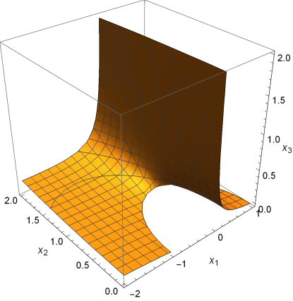
Figure 1: The $2-d$ surface of the Friedmann constraint on the phase space of $x_{1}$, $x_{2}$ and $x_{3}$.

The physical meaning of the constraint is derived from the flatness of the Universe. If the Universe is indeed described by a flat FRW metric -as observations indicate- and contains nothing else than what we already considered, then the fulfillment of the Friedmann constraint is a prerequisite. Its non-fulfillment, on the other hand, would hint as to a non-flat $3-d$ space, or to missing components in the theory, or from a physical point of view, non viability of the corresponding solutions. Setting the latter aside, as we are interested in this specific theory, we should notice that $x_{1}^{2}+x_{2}^{2}+8\sqrt{6}x_{1}x_{3}x_{4}^{2}+x_{5}^{2}<1$ means a FRW Universe with negative spatial curvature (closed FRW cosmologies), whereas $x_{1}^{2}+x_{2}^{2}+8\sqrt{6}x_{1}x_{3}x_{4}^{2}+x_{5}^{2}<1$ means one with negative spatial curvature (open FRW cosmologies).

Generally, we would expect solutions of the system (25-33) to fulfill the Friedmann constraint at all times, otherwise we would regard them as non-physical and unviable. However, we shall see that in the reduced three-dimensional phase space (where $x_{4}=x_{5}=0$) not all solutions respect this constraint. In fact, even when a stable equilibrium point fulfills the constraint, not all trajectories leading to it, fulfill it as well. This could mean that the Einstein-Gauss-Bonnet Universe does not fulfill the Friedmann constraint at all times, and thus it is not described by flat FRW metric throughout all its history, but only at the final attractors. It could also mean, on the other hand, that the assumption of a Universe empty of matter fields is misleading, as we pointed out, since it could guarantee the fulfillment of the Friedmann constraint all the way from the “unviable” initial conditions to the viable fixed point. We discuss and investigate in detail these issues in the following sections.

III.3 The Free Parameters of the Model

The model presented so far contains three free parameters. Two of them are inherited from the assumption of an exponential potential ($\lambda$) and an exponential coupling function ($\mu$), therefore their magnitude and sign follow the following restrictions, namely, they are defined as positive and we know that they must be small and of similar size.

Apart from these, one more free parameter of crucial importance, is the following,

$$m=\dfrac{\dot{H}}{H^{2}}\,.$$

We should remark that this ratio is not generally constant, since the Hubble rate cannot be known in a closed form a priori, that is before the field equations of the theory are solved for specific sources. However, we may notice that a great number of FRW cosmologies -used in both relativistic and modified theories- yield such forms of the Hubble rate, so that this ratio is indeed constant in specific regimes, in other words during specific cosmological eras. Essentially, a constant Hubble rate (as in the de Sitter case) or one such that is $\sim t^{-1}$ (matter- or radiation-dominated eras) will yield a constant $m$, if the barotropic fluids of the Universe are specified, as proved in Section III.A. This can justify our ansatz that this ratio is treated as constant and a free parameter of the system. Our intention is to study the system for different values of $m$, corresponding to different overall behaviors of the space expansion (different cosmological eras), while transitions from one behavior to the next could be perceived as bifurcations in the system.

Another point we need to stress, is the magnitude of the parameter $m$, since the matter and radiation density parameters must be decreasing functions of the $e$-foldings number, as we stated earlier. This results to the restriction $m>-\dfrac{3}{2}$. In fact, it is easy to show that the actual restriction for the values of $m$ is the interval $[-3,0]$. This arises naturally, if we consider the four fundamental solutions of the Friedmann equations in the classical case:

1. Given $w=-1$ or $H(t)=H_{0}$, that corresponds to a de Sitter expanding Universe, then it is easy to calculate that $m=0$.

2. Given $w=\dfrac{1}{3}$ or $H(t)=\dfrac{1}{2t}$, that corresponds to a Universe containing relativistic fluids, or the radiation-dominated era, then $m=-2$.

3. Given $w=0$ or $H(t)=\dfrac{2}{3t}$, that corresponds to a Universe containing non-relativistic (dust) fluids, or the matter-dominated era, then $m=-\dfrac{3}{2}$.

4. Given $w=1$ or $H(t)=\dfrac{1}{3t}$, corresponding to a Universe containing stiff fluids, another era that could be encountered prior or after the inflation, then $m=-3$.

Containing our analysis to these four cases, not only can we discuss all (possible) stages of the Universe evolution in the Standard Cosmological model, but we can also rest assured that $m$ is indeed a constant.

We need to note that various values of the free parameters $\mu$ and $\lambda$ may yield stability or instability of the fixed points corresponding to the various values of the parameter $m$. This fact however may seems to indicate that the values of $\mu$ and $\lambda$ may vary during the various cosmological eras. We need to clarify this issue however, since the phase space analysis we shall perform in the next section focuses on each subspace of the phase space solutions separately. This means that the de Sitter case $m=0$ has to be dealt separately from the $m=-3/2$ matter dominated epoch, so for each case the constraints found for the parameters $\mu$ and $\lambda$ are different in the two cases. Unfortunately there is no way to connect these eras in a physical or mathematical way with the present framework, although in general the couplings may change in an effective way, thus connecting the various cosmological eras, and during each era these may be approximately constant. But as we stated, we do not have this theory at hand, so each study performed in the following, has to be dealt separately from the other studies, and there is no consistent mathematical or physical way in the literature, to our knowledge, that enables one to connect these cosmological eras.

IV The Phase Space of the Model: Analytical Results

Any autonomous dynamical system of the form,

$$x^{\prime}=\mathcal{F}(x)\,,$$

contains a number of invariant structures on the phase space, such that its behavior is determined by them. These can be traced if we consider that the vector field $\mathcal{F}(x)$ is zero or remains constant on them. The first condition, that is $\mathcal{F}(x)=0$, usually reveals the equilibrium points of the system, while the second condition, namely $\nabla\mathcal{F}(x)=0$, reveals limit cycles or other attracting/repelling limit sets, such as for example the stable or unstable manifolds of an equilibrium point. After locating these invariant structures on the phase space of the dynamical system, we may proceed by characterizing their stability, usually by means of the Hartman-Grobman theorem and the linearization of the vector field in small areas around them.

Setting $\mathcal{F}(x)=0$ in our case, we may easily recover four equilibrium points,

$$\begin{split}&P_{0}\left(0,0,0,0,0\right)\;\,,\;\;\;P_{1}\left(-\dfrac{\sqrt{\frac{2}{3}}m}{\mu},0,\dfrac{m(m+3)}{12\mu(m+1)},0,0\right)\;\,,\\ &P_{2}\left(-\dfrac{\sqrt{6}m}{\lambda},-\dfrac{\sqrt{-2m^{2}-6m}}{\lambda},0,0,0\right)\;\;\;\text{and}\;\;\;P_{3}\left(-\dfrac{\sqrt{6}m}{\lambda},\dfrac{\sqrt{-2m^{2}-6m}}{\lambda},0,0,0\right)\,.\end{split}$$ (41)

We observe that all four points collide to $P_{0}$, as $m=0$. Checking if these four points fulfill the Friedmann constraint of Eq. (40), we easily obtain the following conclusions:

1. The point $P_{0}$ is easily proved to not fulfill the constraint, thus it is deemed non-physical.

2. The point $P_{1}$ could fulfill the constraint, if $m\neq 0$ (so it exists apart from $P_{0}$) and

   $$\mu=\pm\dfrac{\sqrt{-2m^{2}(m+5)}}{\sqrt{3(m+1)}}\,;$$

   this however indicates an imaginary $\mu$ for any $m<0$. Thus, the point $P_{1}$ cannot be physical. A hint for determining the importance and viability of this equilibrium point is the fact that $x_{2}^{*}=0$, essentially yielding a zero potential, deeming thus the scalar field to be constant, and $x_{3}^{*}<0$ for all $m<0$, which cannot occur due to our assumptions on the form of $h(\phi)$.

3. Either the point $P_{2}$ or the point $P_{3}$ shall fulfill the constraint. Both cannot be physical at the same time however. If $\lambda=-\sqrt{2m(2m-3)}$, then equilibrium $P_{2}$ is physical, whereas if $\lambda=\sqrt{2m(2m-3)}$, then equilibrium $P_{3}$ is physical. Choosing the latter, so that $\lambda>0$ for $-3\leq m<0$, we easily understand that the point $P_{3}$ is the sole physical equilibrium of the system, much more only when $m<0$ and $\lambda$ is constrained by $m$. The viability of both (unphysical) $P_{2}$ and (physical) $P_{3}$ is intriguing, since $x_{3}^{*}=0$, essentially demanding that either the coupling of the scalar field to the Gauss-Bonnet term is constant, and thus $\mu=0$, or that the Hubble rate tends to zero, for all $-1<m<0$. Given the forms $H(t)\sim t^{-1}$ that we will assume, the latter is indeed possible, allowing us a certain freedom concerning $\mu$, and thus the latter shall be regarded as the one and only true free parameter of the system.

Proceeding with the linearization of the vector field in the vicinity of each fixed point, we may examine their stability.

1. Concerning the point $P_{0}$, the linearized system takes the form

   $$\begin{pmatrix}\xi_{1}^{\prime}\\ \xi_{2}^{\prime}\\ \xi_{3}^{\prime}\\ \xi_{4}^{\prime}\\ \xi_{5}^{\prime}\end{pmatrix}=\begin{pmatrix}-3-m&0&-4\sqrt{6}(1+m)&0&0\\ 0&-m&0&0&0\\ 0&0&2m&0&0\\ 0&0&0&-2-m&0\\ 0&0&0&0&-\dfrac{3}{2}-m\\ \end{pmatrix}\begin{pmatrix}\xi_{1}\\ \xi_{2}\\ \xi_{3}\\ \xi_{4}\\ \xi_{5}\end{pmatrix}\,,$$ (42)

   where $\{\xi_{i}\}$ are small linear perturbations of the dynamical variables around the equilibrium point. The eigenvalues of the system are,

   $$l_{1}=-(3+m)\;\,,\;\;\;l_{2}=-(2+m)\;\,,\;\;\;l_{3}=-\Big{(}\dfrac{3}{2}+m\Big{)}\;\,,\;\;\;l_{4}=-m\;\;\;\text{and}\;\;\;l_{5}=2m\,.$$

   We observe that, for $-3\leq m\leq 0$, all eigenvalues are real, but are subject to a bifurcation. $l_{1}$ is zero for $m=-3$ and turns negative for $-3<m\leq 0$, deeming the direction $v_{1}=\vec{e}_{1}=(1,0,0,0,0)$ initially neutral and attractive afterwards. In the same way $l_{2}$ turns from positive for $-3\leq m<-2$ to negative for $-2<m\leq 0$, thus the manifolds tangent to $v_{2}=\vec{e}_{4}=(0,0,0,1,0)$ turns from unstable to stable. The same occurs for $l_{1}$ in the case $m=-\dfrac{3}{2}$, so that the manifolds tangent to $v_{3}=\vec{e}_{5}=(0,0,0,0,1)$ is initially unstable and shifts to stable when $m<-\dfrac{3}{2}$. Furthermore, the point is subject to two bifurcations for $m=0$. In the case where $m=0$ (de Sitter expansion), $l_{4}=l_{5}=0$, so their respective manifolds are centre manifolds, and thus slow or null evolution of the respective variables occurs on them. When $m<0$, then the manifold tangent to $v_{4}=\Big{(}4\sqrt{\dfrac{2}{3}},0,1,0,0\Big{)}$ becomes stable, while the manifold tangent to $v_{5}=\vec{e}_{2}=(0,1,0,0,0)$ becomes unstable. Thus, the overall behavior of the equilibrium point $P_{0}$ is that of a saddle with attractive and repulsive directions shifting along the values of $m$.

2. Concerning the point $P_{1}$, the linearized system takes the form,

   $$\begin{pmatrix}\xi_{1}^{\prime}\\ \xi_{2}^{\prime}\\ \xi_{3}^{\prime}\\ \xi_{4}^{\prime}\\ \xi_{5}^{\prime}\end{pmatrix}=\begin{pmatrix}-3-m&0&-4\sqrt{6}(m+1)&0&0\\ 0&\dfrac{m\lambda}{3\mu}-m&0&0&0\\ \dfrac{m(m+3)}{2\sqrt{6}(m+1)}&0&0&0&0\\ 0&0&0&-2-m&0\\ 0&0&0&0&-\dfrac{3}{2}-m\\ \end{pmatrix}\begin{pmatrix}\xi_{1}\\ \xi_{2}\\ \xi_{3}\\ \xi_{4}\\ \xi_{5}\end{pmatrix}\,.$$ (43)

   The eigenvalues of the system are,

   $$l_{1} =-(2+m)\;\,,\;\;\;l_{2}=-\Big{(}\dfrac{3}{2}+m\Big{)}\;\,,\;\;\;l_{3}=\dfrac{m(\lambda-3\mu)}{3\mu}\;\,,$$

   $$l_{4} =\dfrac{-3-4m-m^{2}-\mathcal{S}}{2(m+1)}\;\;\;\text{and}\;\;\;l_{5}=\dfrac{-3-4m-m^{2}+\mathcal{S}}{2(m+1)}\;\,,$$

   where $\mathcal{S}=\sqrt{9-34m^{2}-32m^{3}-7m^{4}}$. As in $P_{0}$, for $-3\leq m\leq 0$, two eigenvalues ($l_{1}$ and $l_{2}$) shift from positive to negative at $m=-2$ and $m=-\dfrac{3}{2}$ respectively, thus the manifolds tangent to the directions $v_{1}=\vec{e}_{4}=(0,0,0,1,0)$ and $v_{2}=\vec{e}_{5}=(0,0,0,0,1)$ are initially repulsive and eventually attractive. Eigenvalue $l_{3}$ is subject to two bifurcations, one for $m=0$ and one for $\lambda=3\mu$. In the first case, when $m=0$, the direction of $v_{3}=\vec{e}_{2}=(0,1,0,0,0)$ is neutral, while for $m<0$ and $\lambda>3\mu$ it is attractive. However, when $\lambda=3\mu$, this manifolds becomes neutral again, and when $\lambda<3\mu$ for $m<0$, the manifold tangent to $v_{3}$ becomes unstable. Finally, as long as eigenvalues $l_{4}$ and $l_{5}$ are concerned, both are proved to be real but of different sign in the intervals $-1<m<0$ and $-3<m<-1$, for $\mu>0$; we notice that $l_{4}=l_{5}=0$ for $m=0$ (de Sitter expansion) and $m=-3$ (stiff matter-dominated Universe). Subsequently, the corresponding eigenvectors,

   $$v_{4} =\Bigg{(}\dfrac{\sqrt{6}\left(-3-4m-m^{2}+\sqrt{-(m+1)^{2}\left(7m^{2}+18m-9\right)}\right)}{m^{2}+3m},0,1,0,0\Bigg{)}\;\;\;\text{and}$$

   $$v_{5} =\Bigg{(}-\dfrac{\sqrt{6}\left(-3-4m-m^{2}+\sqrt{-(m+1)^{2}\left(7m^{2}+18m-9\right)}\right)}{m^{2}+3m},0,1,0,0\Bigg{)}\,,$$

   denote an unstable and a stable manifold respectively for $-1<m<0$ and the opposite for $-3<m<-1$, and two centre manifolds for $m=0$ and $m=-3$.

3. Concerning the point $P_{2}$, the linearized system takes the form,

   $$\begin{pmatrix}\xi_{1}^{\prime}\\ \xi_{2}^{\prime}\\ \xi_{3}^{\prime}\\ \xi_{4}^{\prime}\\ \xi_{5}^{\prime}\end{pmatrix}=\begin{pmatrix}-3-m&-2\sqrt{-3(m^{2}+3m)}&-4\sqrt{6}(m+1)&0&0\\ \sqrt{\dfrac{-m^{2}-3m}{3}}&0&0&0&0\\ 0&0&2\left(m-\dfrac{3m\mu}{\lambda}\right)&0&0\\ 0&0&0&-2-m&0\\ 0&0&0&0&-\dfrac{3}{2}-m\\ \end{pmatrix}\begin{pmatrix}\xi_{1}\\ \xi_{2}\\ \xi_{3}\\ \xi_{4}\\ \xi_{5}\end{pmatrix}\,,$$ (44)

   and yields the following eigenvalues,

   $$l_{1} =-(2+m)\;\,,\;\;\;l_{2}=-\Big{(}\dfrac{3}{2}+m\Big{)}\;\,,\;\;\;l_{3}=\dfrac{2m(\lambda-3\mu)}{\lambda}\;\,,$$

   $$l_{4} =\dfrac{-3-m-\sqrt{3\left(3+10m+3m^{2}\right)}}{2}\;\;\;\text{and}\;\;\;l_{5}=\dfrac{-3-m+\sqrt{3\left(3+10m+3m^{2}\right)}}{2}\;\,.$$

   Again, for $-3\leq m\leq 0$, two eigenvalues ($l_{1}$ and $l_{2}$) shift from positive to negative at $m=-2$ and $m=-\dfrac{3}{2}$ respectively, thus the manifolds tangent to the directions $v_{1}=\vec{e}_{4}=(0,0,0,1,0)$ and $v_{2}=\vec{e}_{5}=(0,0,0,0,1)$ are initially repulsive and eventually attractive. The third eigenvalue is zero when $m=0$, or when $m<0$ and $\lambda=3\mu$. This corresponds to a neutrality of the manifold tangent to,

   $$v_{3}=\Bigg{(}-\dfrac{4\sqrt{6}\lambda\left(\lambda-3\mu\right)(1+m)}{-9\lambda\mu+2\lambda^{2}m-15\lambda\mu m+18\mu^{2}m},-\dfrac{2\lambda^{2}(1+m)\sqrt{-2m(m+3)}}{m\left(-9\lambda\mu+2\lambda^{2}m-15\lambda\mu m+18\mu^{2}m\right)},1,0,0\Bigg{)}\,;$$

   this very manifold turns from stable when $\lambda>3\mu$ to unstable when $\lambda<3\mu$. As for the remaining two eigenvalues, these also contain a bifurcation: they are real and negative for $-\dfrac{1}{3}\leq m\leq 0$, complex with negative real parts for $-3<m<-\dfrac{1}{3}$ and zero for $m=-3$. Thus the corresponding eigenvectors,

   $$v_{4} =\Bigg{(}\dfrac{\sqrt{3}\left(-3-m+\sqrt{3\left(3m^{2}+10m+3\right)}\right)}{2\sqrt{-m(m+3)}},1,0,0,0\Bigg{)}\;\,,$$

   $$v_{5} =\Bigg{(}-\dfrac{\sqrt{3}\left(-3-m+\sqrt{3\left(3m^{2}+10m+3\right)}\right)}{2\sqrt{-m(m+3)}},1,0,0,0\Bigg{)}$$

   denote the presence of stable manifolds, either in direct or in oscillatory attraction towards equilibrium $P_{2}$, and a neutral behavior in the case of $m=-3$ (stiff matter-dominated Universe).

4. Finally, in the area of equilibrium point $P_{3}$, the system is linearized as,

   $$\begin{pmatrix}\xi_{1}^{\prime}\\ \xi_{2}^{\prime}\\ \xi_{3}^{\prime}\\ \xi_{4}^{\prime}\\ \xi_{5}^{\prime}\end{pmatrix}=\begin{pmatrix}-3-m&-2\sqrt{-3(m^{2}+3m)}&-4\sqrt{6}(m+1)&0&0\\ \sqrt{\dfrac{-m^{2}-3m}{3}}&0&0&0&0\\ 0&0&2\left(m-\dfrac{3m\mu}{\lambda}\right)&0&0\\ 0&0&0&-2-m&0\\ 0&0&0&0&-\dfrac{3}{2}-m\\ \end{pmatrix}\begin{pmatrix}\xi_{1}\\ \xi_{2}\\ \xi_{3}\\ \xi_{4}\\ \xi_{5}\end{pmatrix}\,,$$ (45)

   and yields the following eigenvalues,

   $$l_{1} =-(2+m)\;\,,\;\;\;l_{2}=-\Big{(}\dfrac{3}{2}+m\Big{)}\;\,,\;\;\;l_{3}=\dfrac{2m(\lambda-3\mu)}{\lambda}\;\,,$$

   $$l_{4} =\dfrac{-3-m-\sqrt{3\left(3+10m+3m^{2}\right)}}{2}\;\;\;\text{and}\;\;\;l_{5}=\dfrac{-3-m+\sqrt{3\left(3+10m+3m^{2}\right)}}{2}\;\,.$$

   It is obvious that whatever said concerning the stability of point $P_{2}$ holds equally for point $P_{3}$. Those two are symmetric over the $x_{2}$ axis, sharing the same stability properties.

From this analysis, it is clear that equilibrium point $P_{0}$ may have up to four attractive directions with two centre manifolds appearing for $m=0$, one for $m=-\dfrac{3}{2}$, one for $m=-2$. This fact, along with its non-viability, mark equilibrium $P_{0}$ as an improbable resolution for the system, while the only case of physical importance in which it is fully hyperbolic is when $m=-1$. In the same manner, equilibrium point $P_{1}$ has at least one unstable manifold and exhibits centre manifolds for $m=0$, one for $m=-\dfrac{3}{2}$, one for $m=-2$ and one for $m=-3$. Another unphysical point, with a subsequent singularity for $m=-1$, cannot be counted as the relaxation point of our system. Finally, equilibria $P_{2}$ and $P_{3}$ are symmetric and under circumstances are globally stable, with all five manifolds being attractive. Such a case is when $m=-1$, however centre manifolds appear for it as well in the physically interesting cases of $m=0$, $m=-\dfrac{3}{2}$, $m=-2$ and $m=-3$.

Discarding the behavior of $x_{4}$ and $x_{5}$ as trivial, we are immediately spared the bifurcations of $m=-\dfrac{3}{2}$ and $m=2$, hence the behavior of the system of Eqs. (25), (27) and (29) is quite normal, proposing that $\lambda>3\mu$ ( that is for $\lambda\gg\mu$, instead of $\lambda=\mu$, which we shall both specifically examine) and $\lambda=\sqrt{2m(2m-3)}$ (to ensure the viability of $P_{3}$). Furthermore, we are able to concentrate on the remaining cases. What we notice is that all other interesting phases of the Universe, stated in section III.C (notably the de Sitter expansion and the stiff matter domination), are cases of bifurcations, where the equilibrium points are non-hyperbolic. Consequently, the behavior of the system cannot be described by the linearization we conducted so far and the need for numerical solutions to reveal the attractor behavior.

Another important feature of the phase space arises when we set $\nabla\mathcal{F}=0$ and solve with respect to the dynamical variables. It is easy to see that,

$$\nabla\mathcal{F}=2\left(m+\sqrt{\dfrac{3}{2}}\mu x_{1}\right)-4m-\dfrac{\lambda x_{1}}{\sqrt{6}}-\frac{13}{2}$$

is zero when $\lambda\neq 6\mu$ and,

$$x_{1}=-\sqrt{\dfrac{3}{2}}\dfrac{(4m+13)}{\lambda-6\mu}\,.$$ (46)

This hypersurface is proved to be an invariant in the phase space when,

$$x_{3}=\dfrac{4m^{2}+25m+39+\lambda x_{2}^{2}(\lambda-6\mu)}{8(m+1)(\lambda-6\mu)}\,.$$ (47)

Eqs. (46) and (47) define an invariant curve in the phase space, one that acts either as a repeller ($\alpha$-limit set) or an attractor ($\omega$-limit set) for the system of Eqs. (25),(27) and (29). It can be proved, rather easily by means of linear perturbations, that it is in fact a repeller, so its practical importance is limited. Furthermore, given $\lambda=6\mu$, both $x_{1}$ and $x_{3}$ tend to infinity, thus the curve is removed from the phase space. One more important element is that, for $-1<m\leq 0$, both $x_{1}$ and $x_{3}$ are negative, so they have no physical meaning whatsoever.

Another interesting feature of the dynamical system is the existence of a curve defined as,

$$C:\;x_{1}=-\dfrac{\sqrt{6}m}{\lambda}\;\;\;\text{and}\;\;\;x_{3}=\dfrac{2m^{2}+6m+\lambda^{2}x_{2}^{2}}{8\lambda(m+1)}\,.$$ (48)

The action of the vector field $\mathcal{F}(x)$ on this curve, is,

$$\mathcal{F}_{1}\dfrac{\partial C}{\partial x_{1}}+\mathcal{F}_{2}\dfrac{\partial C}{\partial x_{2}}+\mathcal{F}_{3}\dfrac{\partial C}{\partial x_{3}}\,,$$ (49)

and is identically zero if $\lambda=3\mu$ or $m=0$, which are the values of the parameters on which bifurcations occur. In other words, we have traced the shifting manifold of equilibrium points $P_{2}$ and $P_{3}$ -which turn to $P_{0}$ for $m=0$. This manifold has been identified as a neutral for $m=0$ or $\lambda=3\mu$, so it functions as a locus of equilibria in these cases.

We may easily apply linear perturbation theory on this curve, as well, leading to the linearized system,

$$\begin{pmatrix}\psi_{1}^{\prime}\\ \psi_{2}^{\prime}\\ \psi_{3}^{\prime}\\ \psi_{4}^{\prime}\\ \psi_{5}^{\prime}\end{pmatrix}=\begin{pmatrix}-m-3&\sqrt{6}\lambda x_{2}&-4\sqrt{6}(1+m)&0&0\\ -\dfrac{\lambda}{\sqrt{6}}x_{2}&0&0&0&0\\ \sqrt{\dfrac{3}{2}}\dfrac{\mu\left(2m^{2}+6m+\lambda^{2}x_{2}^{2}\right)}{4(m+1)\lambda}&0&2\left(m-\dfrac{3m\mu}{\lambda}\right)&0&0\\ 0&0&0&-2-m&0\\ 0&0&0&0&-\dfrac{3}{2}-m\\ \end{pmatrix}\begin{pmatrix}\psi_{1}\\ \psi_{2}\\ \psi_{3}\\ \psi_{4}\\ \psi_{5}\end{pmatrix}\,,$$ (50)

where $\{\psi_{i}\}$ are small linear perturbations of the dynamical variables around the curve $C$. Notice that these perturbations, unlike perturbations around an equilibrium point, dependent on the variable $x_{2}$, which may be treated as a free parameter so long as it is restricted on the curve $C$. The eigenvalues of the system are,

$$l_{1}=-(2+m)\;\,,\;\;\;l_{2}=-\Big{(}\dfrac{3}{2}+m\Big{)}\;\,,\;\;\;l_{3}=\dfrac{\mathcal{R}_{1}}{24(1+m)\lambda}\;\,,\;\;\;l_{4}=\dfrac{\mathcal{R}_{2}}{24(1+m)\lambda}\;\;\;\text{and}\;\;\;l_{5}=\dfrac{\mathcal{R}_{3}}{24(1+m)\lambda}\,,$$

where $\mathcal{R}_{1}$, $\mathcal{R}_{2}$ and $\mathcal{R}_{3}$ are the roots of polynomial

$$\begin{split}&-27648m(m+1)^{3}\lambda^{4}\left(\lambda-3\mu\right)x_{2}^{2}-576(m+1)^{2}\lambda\left(2m^{2}(\lambda-6\mu)+6m(\lambda-6\mu)-\lambda^{2}(\lambda+3\mu)x_{2}^{2}\right)\mathcal{R}-\\ &-24(m+1)\left(\lambda(m-3)-6m\mu\right)\mathcal{R}^{2}+\mathcal{R}^{3}=0\,,\end{split}$$

the first of which is real and negative, while the other two are complex with negative real parts, in the regime of our interest ($-1<m\leq 0$ and $\lambda>6\mu$) and for physical values of the potential ($0\geq x_{2}>10$). As a result, it is easy to conclude that the curve $C$ is an attractive invariant of the system, that offers a multiplicity of stationary solutions in the abnormal cases of $m=0$ and $\lambda=3\mu$.

Aside from the stability of these manifolds, we may also deal with their viability. Setting $x_{1}=-\dfrac{\sqrt{6}m}{\lambda}$, $x_{3}=\dfrac{2m^{2}+6m+\lambda^{2}x_{2}^{2}}{8\lambda(m+1)}$ and $x_{4}=x_{5}=0$ in Eq. (40), we see that,

$$x_{1}^{2}+x_{2}^{2}+8\sqrt{6}x_{1}x_{3}+x_{4}^{2}+x_{5}^{2}=\dfrac{\lambda^{2}(1-5m)x_{2}^{2}-6m^{2}(m+5)}{\lambda^{2}(m+1)}\,,$$

that can equal unity if and only if,

$$x_{2}^{2}=-\dfrac{6m^{2}(m+5)+(m+1)\lambda^{2}}{(5m-1)\lambda^{2}}\,.$$ (51)

Essentially, the system may always end up on the invariant curve $C$, when surpassing a bifurcation -when $m=0$ or $\lambda=3\mu$- but its relaxation is not always physical. In order for the Friedmann constraint to be fulfilled and the viability to be ensured, special initial conditions are needed (a short of fine-tuning) that may lead to specific values of $x_{2}$. As we notice, these values depend on $m$ and $\lambda$, letting $\mu$ as a free parameter. The physical meaning of these is the following: in the de Sitter case of the Universe, or in the case where the potential decreases trice as fast as the coupling increases, with respect to the scalar field, the potential must reach a specific non-zero value so that the Universe will end up on the physical stable de Sitter attractor.

The analysis we performed above is quite rigorous and mathematically rigid, however we need to enlighten the physics of the phase space with numerical analysis. In this way we may visualize all the invariant manifolds and curves we discovered in this section. This is compelling for a more persuasive treatment of the problem, and it is the subject of the next section.

V The Phase Space of the Model: Numerical solutions

In order to better understand the phase space structure of the Einstein-Gauss-Bonnet models, we shall numerically integrate the differential equations (25), (27) and (29) for a number of cases with physical interest, as stated above. The integration of Eqs. (32) and (33) is conducted analytically, so they will not trouble us. The Universe should not be considered vacuum, with the presence of matter fields being mimicked by the modification of gravity along with the specific choice of the Hubble rate, and thus of the parameter $m$, as usually; this would lead to the misperception of certain solutions. We need to keep in mind that only the reduced phase space is studied here, hence specific trajectories that appear to be unviable could be viable -and the vice versa. Whenever necessary, we shall comment on the behaviour of $x_{4}$ and $x_{5}$, though this behavior depends largely on the Hubble rate, rather than that of the mass-energy densities.

For a specific case, the integration of the “inverse problem” ($x^{\prime}=-\mathcal{F}(x)$) was also utilized, in order to find special initial conditions that are needed to realize a specific behaviour.

V.1 de Sitter expanding Universe: $m=0$

Setting $m=0$, then Eqs. (25), (27) and (29) reduce to,

$$x_{1}^{\prime} =-3x_{1}+\dfrac{\sqrt{6}}{2}\lambda x_{2}^{2}-4\sqrt{6}x_{3}\;\,,$$ (52)

$$x_{2}^{\prime} =-\dfrac{\sqrt{6}}{2}\lambda x_{1}x_{2}\;\;\text{and}$$ (53)

$$x_{3}^{\prime} =\dfrac{\sqrt{6}}{2}\mu x_{1}x_{3}\,.$$ (54)

The above dynamical system has one equilibrium point, $P_{0}$, that has been proved to possess one stable and two centre manifolds. Furthermore, there exists the curve $C:\;x_{3}=\dfrac{\lambda}{8}x_{2}^{2}$ for $x_{1}=0$, which is an attractor for the solutions of the system, one of the centre manifolds of point $P_{0}$. The attraction towards curve $C$ occurs by means of oscillations for $x_{2}>\dfrac{3}{2\sqrt{\lambda^{2}+3\lambda\mu}}$, and by means of direct attraction for $x_{2}<\dfrac{3}{2\sqrt{\lambda^{2}+3\lambda\mu}}$.

What we actually expect is that all solutions of the system will reach this attractor and remain fixed on some point of it. The exact point is not important, except for $x_{1}^{*}=0$, $x_{2}^{*}=1$ and $x_{3}^{*}=\dfrac{\lambda}{8}$, that fulfills the Friedmann constraint. Of course, this is only one of the infinite points on which the dynamical system may be attracted to. In order to trace initial conditions that lead to the physical point of curve $C$, we employed the technique of the “inverse problem” and located one trajectory leading to this point -the trajectory colored dark green in each subplot of Fig. 2. It is worth noting that, despite all other trajectories -the black ones- have been derived from initial conditions that respected the Friedmann constraint (Eq. (40), this particular trajectory -and any similar- initiates from sections of the phase space that do not fulfill the constraint. This is an important feature to be noticed.

In this case, $\lambda=\sqrt{2m(2m-3)}=0$ is of little physical meaning (constant potential over the scalar field), thus it will not be used. On the contrary, we chose four cases that could be of interest: $\lambda=3\mu$, a case of bifurcations for $m\neq 0$; $\lambda=6\mu$ and $\lambda=\mu$, before and after the bifurcation, and $\lambda\gg\mu$, that is expected to have some physical meaning (a potential evolving faster over $\phi$ than the coupling function $h(\phi)$ to the Gauss-Bonnet term). All cases yielded similar results, with all the solutions reaching normally the attraction curve $C$. Only in the last case, the attractions were direct, instead of oscillatory, due to the relationship between $\lambda$ and $\mu$.

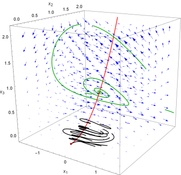
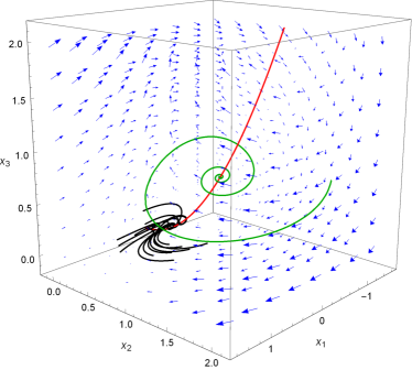
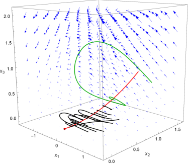
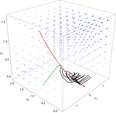
Figure 2: The phase space of $x_{1}$, $x_{2}$ and $x_{3}$ for the de Sitter expanding Universe, for $\lambda=3\mu$, $\lambda=6\mu$, $\lambda=\mu$ and $\lambda\gg\mu$ (from top-left to bottom-right). Blue arrows denote the vector field, black lines denote numerical solutions of the system; the red curve stands for the centre manifold $x_{3}=\dfrac{\lambda}{8}x_{2}^{2}$ and the equilibrium point $P_{0}$ is marker dark red.

During this era, both $x_{4}$ and $x_{5}$ are decreasing fast towards their equilibrium values $x_{4}^{*}=x_{5}^{*}=0$.

V.2 Radiation-dominated Universe: $m=-2$

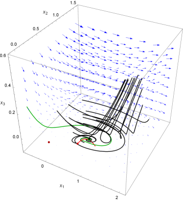
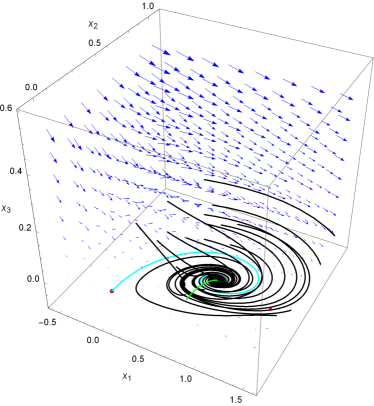
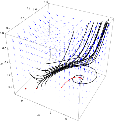
Figure 3: The phase space of $x_{1}$, $x_{2}$ and $x_{3}$ for the radiation-dominated Universe, for $\lambda=3\mu$, $\lambda=6\mu$, $\lambda=\mu$ and $\lambda\gg\mu$ (from top-left to bottom-right). Blue arrows denote the vector field, black lines denote numerical solutions of the system; the red curve stands for the unstable manifold and the green curve for the stable manifold, while the cyan curve depicts the heteroclinic curve from $P_{0}$ to $P_{3}$. The equilibrium points are marked dark red if they are unviable and dark green if they are viable.

Setting $m=-2$, then Eqs. (25), (27) and (29) reduce to,

$$x_{1}^{\prime} =-x_{1}+\dfrac{\sqrt{6}}{2}\lambda x_{2}^{2}+4\sqrt{6}x_{3}\;\,,$$ (55)

$$x_{2}^{\prime} =-x_{2}\Bigg{(}\dfrac{\sqrt{6}}{2}\lambda x_{1}-2\Bigg{)}\;\;\text{and}$$ (56)

$$x_{3}^{\prime} =x_{3}\Bigg{(}\dfrac{\sqrt{6}}{2}\mu x_{1}-2\Bigg{)}\,.$$ (57)

These equations exhibit all four equilibrium points we have mentioned. Point $P_{0}$ possesses two stable and one unstable manifolds. Point $P_{1}$ possesses one stable and one unstable manifold, while the third, tangent to $\vec{e}_{2}=(0,1,0)$, shifts from stable to unstable as $\lambda=3\mu$; finally, points $P_{2}$ and $P_{3}$ yield two complex eigenvalues with negative real parts (so attraction with oscillations) and a third real eigenvalue that shifts from negative to positive as $\lambda=3\mu$. As a result, we shall use the same values of $\lambda$ as with the previous case ($m=0$). Furthermore, in the last case $\lambda=\sqrt{2m(2m-3)}=2\sqrt{7}$ is chosen as to ensure the viability of point $P_{3}$. We should notice that the curve $C$ takes the form,

$$x_{3}=\dfrac{4-\lambda^{2}x_{2}^{2}}{8\lambda}\,,$$ (58)

and acts either as stable, centre or unstable manifold for the system, depending on the relationship between $\lambda$ and $\mu$. The stable cases are denoted as green curves, whereas the unstable ones are denoted as red in Fig. 3. We also notice the existence of a heteroclinic curve leading from equilibrium $P_{0}$ to equilibrium $P_{3}$. This curve is painted cyan in two of the subplots of Fig. 3.

In the case of $\lambda=3\mu$ (the top-left subplot of Fig. 3), where the manifold is neutral, we solved the “inverse problem” tracing a trajectory that reaches a physical point in the phase space, one for which $x_{1}=\dfrac{2\sqrt{6}}{\lambda}$ , $x_{2}=\dfrac{1}{\lambda}\sqrt{\dfrac{24+\lambda^{2}}{13}}$ and $x_{3}=\dfrac{28-\lambda^{2}}{104\lambda}$; this trajectory is marked dark green in the first subplot of Fig. 3. Once more, while all numerical solutions were derived starting from initial conditions that fulfilled the Friedmann constraint, this very trajectory originates from sections of the phase space that do not fulfill the constraint, neither do they contain physical value for all dynamical variables. We also met this peculiar situation in the de Sitter cosmology case, so it seems there is some universal behaviour for the exponential Einstein-Gauss-Bonnet models. What was expected from the qualitative analysis and confirmed from the numerical integrations is that only at specific cases there exists a viable and stable equilibrium point where the system may eventually be attracted to, after relatively large oscillations of some phase space variables.

Cases may exist -such as when $\lambda<3\mu$- that the equilibrium point will exist but it will be neither viable, nor stable, hence solutions of the model are repelled far away from it. Furthermore, two important comments are in order, which we derived from our numerical investigation, which are the following:

• The convergence to the equilibrium point, if it is stable, occurs relatively fast, within $20$ $e$-folds. The divergence, on the other hand, if the equilibrium point is not stable, is even faster, as some dynamical variables reach extremely large values within $5$ $e$-folds.

• Even when the initial values of variables $x_{1}$, $x_{2}$ and $x_{3}$ along the equilibrium they reach, fulfill the Friedmann constraint, the same is not necessary throughout the whole trajectory; taking into account the evolution of $x_{4}$ and $x_{5}$ may solve this paradox.

In this case, we should again note, $x_{4}$ is constant while $x_{5}$ increases as a function of the $e$-foldings number, diverging from its equilibrium value $x_{5}^{*}=0$. This should be attributed either to the behaviour of the Hubble rate, or to the fact that baryonic matter, especially cold dark matter, is known to evolve and form structures during the radiation-dominated phase of the Universe.

V.3 Matter-dominated Universe: $m=-\dfrac{3}{2}$

The same behaviour holds true, more or less, in the case the Universe is dominated by matter. Setting $m=-\dfrac{3}{2}$, then Eqs. (25), (27) and (29) reduce to

$$x_{1}^{\prime} =-\dfrac{3}{2}x_{1}+\dfrac{\sqrt{6}}{2}\lambda x_{2}^{2}+2\sqrt{6}x_{3}\;\,,$$ (59)

$$x_{2}^{\prime} =-x_{2}\Bigg{(}\dfrac{\sqrt{6}}{2}\lambda x_{1}-\dfrac{3}{2}\Bigg{)}\;\;\text{and}$$ (60)

$$x_{3}^{\prime} =x_{3}\Bigg{(}\dfrac{\sqrt{6}}{2}\mu x_{1}-\dfrac{3}{2}\Bigg{)}\,.$$ (61)

Again, these equations exhibit all four equilibrium points we have mentioned. Point $P_{0}$ possesses two stable and one unstable manifolds; point $P_{1}$ possesses one stable and one unstable manifold, while the third, tangent to $\vec{e}_{2}=(0,1,0)$, shifts from stable to unstable as $\lambda=3\mu$; finally, points $P_{2}$ and $P_{3}$ yield two complex eigenvalues with negative real parts (so attraction with oscillations) and a third real eigenvalue that shifts from negative to positive as $\lambda=3\mu$. The cases of $\lambda$ and $\mu$ used prior, will be used here as well. Furthermore, in the last case $\lambda=\sqrt{2m(2m-3)}=3\sqrt{2}$ is chosen as to ensure the viability of point $P_{3}$.

We should notice that the curve $C$ takes the form

$$x_{3}=\dfrac{\frac{9}{2}-\lambda^{2}x_{2}^{2}}{4\lambda}\,,$$ (62)

and acts either as stable, centre or unstable manifold for the system, depending on the relationship between $\lambda$ and $\mu$. The stable cases are denoted as green curves, whereas the unstable ones are denoted as red in Fig. 4. We also notice the existence of a heteroclinic curve leading from equilibrium $P_{0}$ to equilibrium $P_{3}$. This curve is appears in cyan color in two of the subplots of Fig. 4.

In the case of $\lambda=3\mu$ (the top-left subplot of Fig. 4, where the manifold is neutral, we solved the “inverse problem” tracing a trajectory that reaches a physical point in the phase space, with $x_{1}=\dfrac{3\sqrt{6}}{2\lambda}$ , $x_{2}=\dfrac{1}{34}\left(\dfrac{189}{\lambda^{2}}+2\right)$ and $x_{3}=-\dfrac{4\lambda^{4}-4446\lambda^{2}+35721}{4624\lambda^{3}}$. This trajectory is marked dark green in the first subplot of Fig. 4. Its initiation, unlike all other cases -marked black- does not fulfill the Friedmann constrains.

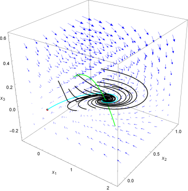
Figure 4: The phase space of $x_{1}$, $x_{2}$ and $x_{3}$ for the matter-dominated Universe, for $\lambda=3\mu$, $\lambda=6\mu$, $\lambda=\mu$ and $\lambda\gg\mu$ (from top-left to bottom-right). Blue arrows denote the vector field, black lines denote numerical solutions of the system; the red curve stands for the unstable manifold and the green curve for the stable manifold, while the cyan curve depicts the heteroclinic curve from $P_{0}$ to $P_{3}$; the equilibrium points are marked dark red if they are unviable and dark green if they are viable.

In fact, whatever said in the case of the radiation-dominated Universe holds equally for the matter-dominated. The only difference concerns the behaviour of discarded variables $x_{4}$ and $x_{5}$. Here, $x_{5}$ is constant while $x_{4}$ decreases over the $e$-foldings number, eventually reaching its equilibrium value $x_{4}^{*}=0$; both evolutions are in accordance to the Standard Cosmological model, whereas the density of radiation decreases during the matter-dominated era.

V.4 Stiff Matter-dominated Universe: $m=-3$

The case of stiff matter, although more bizarre, seems far more interesting, since the phase space alters significantly. Setting $m=-3$ to Eqs. (25), (27) and (29), we obtain

$$x_{1}^{\prime} =\dfrac{\sqrt{6}}{2}\lambda x_{2}^{2}+8\sqrt{6}x_{3}\;\,,$$ (63)

$$x_{2}^{\prime} =-x_{2}\Bigg{(}\dfrac{\sqrt{6}}{2}\lambda x_{1}-3\Bigg{)}\;\;\text{and}$$ (64)

$$x_{3}^{\prime} =x_{3}\Bigg{(}\dfrac{\sqrt{6}}{2}\mu x_{1}-3\Bigg{)}\,.$$ (65)

These equations contain in fact three of the original equilibrium points, as $P_{2}$ and $P_{3}$ coincide. However, it contains a peculiar solution, in the form of $x_{2}^{*}=0$ and $x_{3}^{*}=0$, which eventually means that the $x_{1}$ axis contains infinite equilibrium points (including $P_{0}$, $P_{1}$ and $P_{2}=P_{3}$). It is relatively easy to see that the eigenvector $v_{1}=\vec{e}_{1}=(1,0,0)$ is always a centre manifold for any of the infinite equilibrium points on this axis. Furthermore, the eigenvector $v_{2}=\vec{e}_{2}=(0,2,0)$ is found to be tangent to a stable manifold for $\lambda>\mu$, a centre manifold for $\lambda=3\mu$ and an unstable manifold for $\lambda<3\mu$. It is also an attractor for any $x_{1}>\dfrac{3\sqrt{6}}{\lambda}$. Finally, the third direction, found to be tangent to $v_{3}=\Big{(}-\sqrt{\dfrac{2}{3}}\dfrac{4\lambda}{\lambda-3\mu},0,1\Big{)}$ is attractive towards the $x_{1}$ axis for any $\lambda>3\mu$.

The curve $C$, usually denoting a manifold of the viable equilibrium point $P_{3}$, though it exists, it is usually reduced to a simple line. The same holds for the heteroclinic curve connecting $P_{1}$ with $P_{3}$. Though it still exists, it has been reduced to a straight line across the $x_{1}$ axis. The phase space contains least one centre manifold along the $x_{1}$ axis.

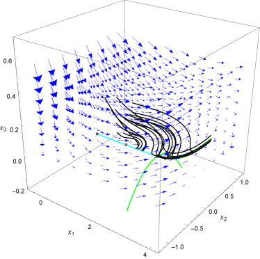
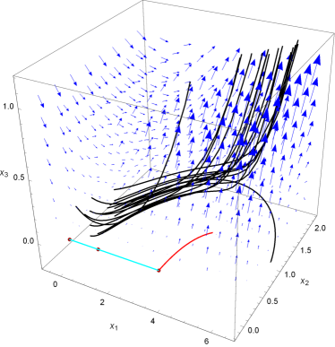
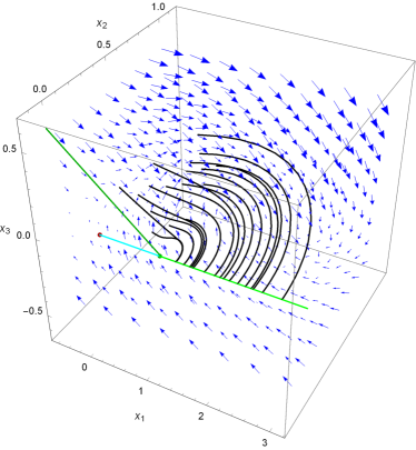
Figure 5: The phase space of $x_{1}$, $x_{2}$ and $x_{3}$ for the stiff matter-dominated Universe, for $\lambda=3\mu$, $\lambda=6\mu$, $\lambda=\mu$ and $\lambda\gg\mu$ (from top-left to bottom-right). Blue arrows denote the vector field, black lines denote numerical solutions of the system; the red curve stands for the unstable manifold and the green curve for the stable manifold, while the cyan curve depicts the heteroclinic curve from $P_{0}$ to $P_{3}$; the equilibrium points are marked dark red if they are unviable and dark green if they are viable.

We should especially focus on the case where $\lambda=\sqrt{2m(2m-3)}=3\sqrt{6}$ -depicted in the fourth subplot of Fig. 5- that ensures the viability of equilibrium $P_{2}=P_{3}$. Here, trajectories begin an oscillatory motion around equilibrium $P_{2}=P_{3}$, which eventually leads them to a halt as they meet the horizontal axis for some $x_{1}>\dfrac{3\sqrt{6}}{\lambda}$, captured by the centre manifold. Hence, unlike all four previous models examined, in the case of a stiff matter-dominated Universe, there is no condition to ensure that the viable equilibrium is also stable and generally reached by the solutions of the system. Solving the “inverse problem”, we manage to trace a trajectory leading to the equilibrium $P_{2}=P_{3}$, however, as with other such case, it does not originate from a physically meaningful section of the phase space, neither does it fulfill the Friedmann constraint all the way through from its beginning -the trajectories obtained by the “inverse problem” are painted dark green in the first and the fourth subplot of Fig. 5.

Once more, both $x_{4}$ and $x_{5}$ increase over the $e$-foldings number, diverging from the equilibrium $x_{4}^{*}=x_{5}^{*}=0$. This behaviour is hard to explain, though it probably relies on the behaviour of the Hubble rate, or the fact that stiff matter dominates the Universe, rendering both dust and radiation unstable.

VI Analysis of the Results and Concluding Remarks

Let us now elaborate on the results and discuss the outcomes of the analysis performed in the previous sections. We have seen that the dynamical system contains up to four equilibrium points, only one of which is viable and physically meaningful under specific conditions. It also contains at least one invariant submanifold that may shift from unstable to stable, either repelling or attracting solutions from/to the viable equilibrium point, or in specific cases turn to centre manifold, attracting all solutions on it. Finally, it contains a heteroclinic trajectory leading from an unviable equilibrium to the viable one. Our numerical analysis also showed that the equilibrium is reached relatively fast (within $20$ to $30$ $e$-folds, for all examined cases), while achieving a viable equilibrium is not at all secured, even if the initial conditions fulfill the Friedmann constraint for the reduced phase space of $x_{1}$, $x_{2}$ and $x_{3}$. In sharp contrast, it is shown that the viable equilibrium may be reached by trajectories that do not fulfill the Friedmann constraint when $x_{4}=x_{5}=0$ is imposed and contain non-physical values for at least one dynamical variable, namely a negative value for $x_{2}$ or $x_{3}$.

Combining these elements with the theory developed in Section II and the definitions of the dynamical variables in Eq. (22), we may provide a clue as to the viability of the original theory, at least in the specific cases of FRW cosmologies studied here.

First of all, we should make clear that the viable equilibrium $P_{3}$ is proved to be stable for most of the cases, provided that $\lambda=\sqrt{2m(2m-3)}$ (condition of viability) and $\lambda>3\mu$ (condition of stability). Hence it may attract solutions from the whole phase space. Essentially, the cosmological model under examination may be attracted on this stationary state after evolving for some time, due to the presence of the potential and the Gauss-Bonnet term. As for the meaning of this equilibrium, one should state that both the behaviour of $x_{1}$ and $x_{2}$ seems normal. They denote,

$$\dfrac{1}{2}\dot{\phi}^{2}=\dfrac{18}{\lambda^{2}}\Big{(}\dfrac{\dot{H}}{H}\Big{)}^{2}=\dfrac{18}{\lambda^{2}t^{2}}\;\;\;\text{and}\;\;\;V(\phi)=\dfrac{6}{\lambda^{2}}\Bigg{(}\Big{(}\dfrac{\dot{H}}{H}\Big{)}^{2}-3\dfrac{\dot{H}}{H}\Bigg{)}=\dfrac{6}{\lambda^{2}}\Big{(}\dfrac{1}{t^{2}}-\dfrac{3}{t^{2}}\Big{)}\,,$$

in other words, that the kinetic term and the potential of the scalar field must evolve according to time as the evolution of the system ceases; their evolution is proved to be rather trivial, since both tend to zero, for a large time-scale. Yet, the value of $x_{3}$ comes quite as peculiar, since it demands that the coupling function turns constant. This appears reasonable at first, since it states that at equilibrium, the Gauss-Bonnet term is decoupled from the scalar field, or even nullified, however, it turns out to be a non-physical argument. To achieve this, we need either $h_{0}=0$ or $\mu=0$, both of which cannot occur. On the one hand, setting $\mu=0$ leads to the emergence of poles on the phase space, on the other hand, either $h_{0}=0$ or $\mu=0$ means that the coupling function should be zero from the beginning, hence the scalar field should be decoupled from the Gauss-Bonnet term. This immediately sets us off with respect to our original theoretical streamline, since we no longer deal with an Einstein-Gauss-Bonnet model.

The only physical explanations for it would be that either the assumption of an exponential coupling function was a rather misleading one, or that the quadratic curvature terms should vanish at some point, leading to the nullifying of the coupling, without the necessity of $\mu$ turning to zero. Both of these explanations, however, fall beyond the reach of the examined models.

A second interesting case is that of the centre manifold appearing at $m=0$ or $\lambda=3\mu$, in the form of the curve $C$. In this case,

$$\dfrac{1}{2}\dot{\phi}^{2}=\dfrac{18}{\lambda^{2}}\Big{(}\dfrac{\dot{H}}{H}\Big{)}^{2}\;\,,\;\;\;V(\phi)=\dfrac{18\dot{H}^{2}\big{(}\dot{H}+5H^{2}\big{)}+H^{4}\big{(}\dot{H}+H^{2}\big{)}\lambda^{2}}{H^{2}\big{(}5\dot{H}-H^{2}\big{)}\lambda^{2}}\;\;\;\text{and}\;\;\;h(\phi)=\dfrac{4\dot{H}^{2}-6\dot{H}H^{2}-H^{4}\lambda}{8\lambda\mu\big{(}5\dot{H}-H^{2}\big{)}}\,,$$

so that the kinetic term, the potential and the coupling function end up to some non-zero values, all of them being physical. This may occur in the following two cases:

• If $m=0$, so that $H=H_{0}$ and $\dot{H}=0$, meaning that

  $$\dfrac{1}{2}\dot{\phi}^{2}=0\;\,,\;\;\;V(\phi)=-H_{0}^{2}\;\;\;\text{and}\;\;\;h(\phi)=\dfrac{H_{0}^{2}}{8}\dfrac{\lambda}{\mu}\,.$$

  In this case, the kinetic term vanishes, so the evolution of the scalar field ceases, but neither the potential nor the coupling to the Gauss-Bonnet term vanish. Essentially, this may occur during the early- or late-time accelerating expansion of the Universe, where the scalar field and quadratic curvature terms may indeed give rise to the specific behaviour. If it is so, then when the system is at the final attractor, the Hubble rate remains constant, so the expansion remains accelerating. Furthermore, neither the Gauss-Bonnet term, nor the scalar field may completely vanish, if the accelerating expansion does not come to a halt. The scalar field turns constant and -along with the Gauss-Bonnet term, or even on its own- acts as a Cosmological constant.

• If $\lambda=3\mu$. In this case, $\lambda$ may be arbitrary, since the viability of the equilibrium does not depend on it, however, it must be triple in magnitude in comparison to $\mu$. This equality means that, given an increasing value of the scalar field, the potential must decrease in a triple rate to that of the increase of the coupling function -and the opposite, for a decreasing scalar field. In other words, the potential must vanish prior to the coupling of the scalar field to the quadratic curvature terms. Consequently, quadratic curvature may survive outside the inflationary era and during the radiation-dominated and matter-dominated eras, where it should not be active. This mechanism, however, is capable of retaining the quadratic curvature terms long after the inflation and re-triggering them at late-times, so as to give the observed late-time accelerating expansion.

These may sound a good arguments in support of the Einstein-Gauss-Bonnet theory, providing that an inherent mechanism exists that would nullify the quadratic curvature coupling to the scalar field during radiation- and matter-dominated eras and re-trigger it during the late-time acceleration. In this manner, both early- and late-time dynamics of the Universe could be derived from the same model. However, the analysis of the radiation- and matter-dominated eras, especially the stability of equilibrium point $P_{3}$, complicate this estimation. As we demonstrate afterwards the survival of the quadratic curvature coupling to the scalar field is seriously questioned for the classical eras.

Third, concerning the specific values of $\lambda$ and $\mu$ in all cases we must have $m<0$, so that equilibrium point $P_{3}$ is both stable and physical. it turns out that $\lambda$ must track the Hubble rate, through the condition $\lambda=\sqrt{2m(2m-3)}$ to retain the viability of the equilibrium, which eventually means that the potential must be somehow interacting with the expansion of the $3-d$ space. Furthermore, to ensure the stability of the equilibrium, another condition is imposed, $\lambda>3\mu$, which eventually means that $\mu$ is a free parameter as long as it is smaller enough than $\lambda$. In this way, we ensure that the coupling function increases less rapidly than the potential, given an increasing scalar field, and the quadratic curvature terms may remain coupled to the scalar field after the early stages of the Universe throughout its whole evolution, only to be re-triggered in the late-time.

Fourth, a heteroclinic trajectory exists in the phase space, leading from the unviable equilibrium point $P_{0}$ to the viable equilibrium point $P_{3}$, retaining the value of variable $x_{3}$ equal to zero. This might be the sole most important trajectory in the phase space, despite the fact that it leads to an ab initio nihilism of the Gauss-Bonnet term and/or its coupling to the scalar field. In fact, setting $x_{3}=0$ and remaining on the $x_{1}-x_{2}$ plane, we are dealing with the simple form of a minimally coupled scalar-tensor theory. This plane is perhaps more important in cases where $m\neq 0$ -the case where the two equilibrium points are distinct and the heteroclinic curve actually exists. In such cases, we may assume that the quadratic curvature terms have vanished, or equivalently that the scalar field has been decoupled from the Gauss-Bonnet term. Hence, $\mu$ can be chosen to be zero, while $\lambda\neq 0$. In this case, the phase space would be further reduced on the $x_{1}-x_{2}$ plane, where both the unviable equilibrium $P_{0}$ and the viable equilibrium $P_{3}$ lie, along with the heteroclinic curve among them. Subsequently, all we should discuss about would concern the simplest form of a scalar-tensor theory, maintaining the scalar field and its potential throughout the radiation-dominated and matter-dominated eras, so that it would re-emerge in the late-time era, and cause the accelerating expansion. In such a scenario, the transcendence from the early Universe (de Sitter case) to the later stages of evolution (radiation-dominated and matter-dominated Universe) would demand a double bifurcation. Firstly, $m$ should turn from zero to negative, and secondly, $\mu$ should turn from positive to zero. If so, then an early-time accelerating expansion governed by both the scalar field and the Gauss-Bonnet term, would lead to standard cosmologies with a latent scalar field, and eventually to a late-time accelerating expansion, governed solely by the scalar field. The existence of the heteroclinic trajectory, repelling solutions from $P_{0}$ and attracting them to $P_{3}$, is vital for all models where $m<0$, since it denotes the slow emergence of the scalar field. As the dynamical variables rise from zero to $x_{1}^{*}=-\sqrt{\dfrac{6m^{2}}{2m^{2}-6m}}$ and $x_{2}^{*}=\sqrt{-\dfrac{m+3}{m-3}}$, the kinetic term and the potential of the scalar field turn from zero to non-zero. At the same time, the non-accounted-for variables $x_{4}$ and $x_{5}$ evolve according to Eqs. (37), namely $x_{4}$ increasing and $x_{5}$ remaining constant during the radiation-dominated era, or $x_{4}$ remaining constant and $x_{5}$ decreasing towards $x_{5}^{*}=0$ during the matter-dominated era.

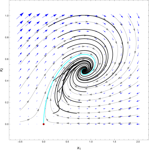
Figure 6: The projection of the phase space on the $x_{1}$-$x_{2}$ plane (for $x_{3}=0$). Blue arrows denote the vector field, while grey streamlines denote possible evolutions on the plane; the equilibrium points $P_{1}$ and $P_{2}$ are the crimson and green spots, while the cyan curve connecting them stands for the heteroclinic trajectory. The black curves are projections of the numerical solutions of the complete system; notice that after a brief time, they fall on the plane and follow its streamlines.

Last, but not least, we should also refer to what appears to be a problem of the non-fulfillment of the Friedmann constraint throughout the whole evolution of the dynamical variables from their initial state, until the attainment of an equilibrium -either $P_{3}$ or the curve $C$. This is, in fact, a very interesting point, since it allows us to consider two following two facts that have not been clarified so far, one of them being the separate evolution of $x_{4}$ and $x_{5}$, the other the question of the flatness of the Universe.

• What seems as logical at first, is that our assumption of the flatness of the Universe was wrong and perhaps a non-prerequisite. This contradicts both observations confirming the flatness of the Universe present time. However, imposing $x_{4}=x_{5}=0$, hence a vacuum Universe, in the case of radiation- and matter-dominated eras ($m=-2$ and $m=-3/2$ respectively), where matter fields could be mimicked by the modification of gravity, as it is accustomed in the literature, leads to the paradox of trajectories that are unviable at their initial state, or during their evolution, but converge to a viable equilibrium point, namely $P_{3}$. It is furthermore proved that all these trajectories surpass a stage for which $x_{1}^{2}+x_{2}^{2}+8\sqrt{6}x_{1}x_{3}<1$, namely the Universe, that eventually becomes flat, needs not to be flat throughout its full history, but can realize positive spatial curvature that decreases to zero as the scalar field and the matter fields emerge and evolve to finally reach equilibrium $P_{3}$. This is a generally unacceptable result in relativistic cosmologies, that should be avoided in modified theories, as well, probing for a different resolution of the paradox.

• What we actually assumed to derive this paradox was a Universe empty of matter fields, a case usually considered yet easy to discharge as unrealistic. Considering ourselves free to omit variables $x_{4}$ and $x_{5}$, due to the separability and integrability of Eqs. (32) and (33), we practically fell pray to this paradox. Such an omission is mathematically justified, due to the form of our dynamical system, yet it is not necessarily justified from a physical standpoint, especially when considering the Friedmann constraint. Even if for some equilibrium point, where $x_{4}^{*}=x_{5}^{*}=0$, the Friedmann constraint is fulfilled, it does not mean that the constraint will be fulfilled for all trajectories attaining the equilibrium -hence for all evolutions realizing this Universe- without taking into account the non-zero values of $x_{4}$ and $x_{5}$, prior to their nihilism. Eventually, the non-fulfillment of the reduced Friedmann constraint for trajectories that reach a viable equilibrium point can be resolved if we take into account the evolution of $x_{4}$ and $x_{5}$ as they decrease towards their equilibrium values. Notably, all trajectories that yield $x_{1}^{2}+x_{2}^{2}+8\sqrt{6}x_{1}x_{3}<1$ could easily yield $x_{1}^{2}+x_{2}^{2}+8\sqrt{6}x_{1}x_{3}+x_{4}^{2}+x_{5}^{2}=1$ if Eqs. (32) and (33) were taken into account. It is, in fact, the combined behaviour of $x_{1}$, $x_{2}$, $x_{4}$ and $x_{5}$ that may fulfill the Friedmann constraint and ensure physical solutions for the reduced scalar-tensor theory.

To conclude, we may state that the phase space analysis of the Einstein-Gauss-Bonnet cosmological models revealed a great number of interesting facts about the theory overall and its ability to describe the actual evolution of the Universe. It is sound to assume that it offers a viable and stable equilibrium point, only if certain conditions are fulfilled for the free parameters of the theory. Furthermore, while the de Sitter case gives rise to a viable inflationary scenario, the non-fulfillment of the Friedmann constraint results to the necessity of matter fields or of an open Universe during the early and very early Universe; of these two, the former sounds as the more reasonable choice, deeming unsafe to treat such cosmological models as a vacuum Universe, even when the Gauss-Bonnet invariant can mimic the effects of matter fields. Finally, the transition from the de Sitter inflationary phase to the later stages of evolution, such as the radiation-dominated and the matter-dominated Universe, should be followed by a second transition that would decouple the Gauss-Bonnet term from the scalar field and essentially nullify the quadratic curvature terms. In this case, the Einstein-Gauss-Bonnet theory seems more like a predecessor to the scalar-tensor theory that may describe the later phase of the Universe, up to the late-time accelerating expansion. In fact, it is a conclusion of our analysis, that the scalar field turns constant for large time-scales, if the equilibrium point $P_{3}$ is attained in radiation-dominated and matter-dominated eras, justifying for the transition to the late-time phase of accelerating expansion.

The case of stiff matter dominating the Universe is highly peculiar and degenerate and can be considered as highly improbable, as in the Standard Cosmological model. The non-minimal coupling of the scalar field to the Ricci scalar curvature should also be taken into consideration, but that is rather left for a future work. Another element in need of further study is the phase transition and decoupling of the scalar field from the quadratic curvature, an element that might be shredded with more light in the view of extensions of Einstein-Gauss-Bonnet models.

References

- (1) D. Lovelock, J. Math. Phys. 12 (1971) 498. doi:10.1063/1.1665613
- (2) M. Farhoudi, Gen. Rel. Grav. 41 (2009) 117 doi:10.1007/s10714-008-0658-9 [gr-qc/9510060].
- (3) S. Nojiri, S. D. Odintsov and V. K. Oikonomou, Phys. Rept. 692 (2017) 1 doi:10.1016/j.physrep.2017.06.001 [arXiv:1705.11098 [gr-qc]].
- (4) S. Nojiri, S.D. Odintsov, Phys. Rept. 505, 59 (2011);
- (5) S. Nojiri, S.D. Odintsov, eConf C0602061, 06 (2006) [Int. J. Geom. Meth. Mod. Phys. 4, 115 (2007)]. [arXiv:hep-th/0601213];
- (6) S. Capozziello, M. De Laurentis, Phys. Rept. 509, 167 (2011) [arXiv:1108.6266 [gr-qc]]. V. Faraoni and S. Capozziello, Fundam. Theor. Phys. 170 (2010). doi:10.1007/978-94-007-0165-6
- (7) A. de la Cruz-Dombriz and D. Saez-Gomez, Entropy 14 (2012) 1717 doi:10.3390/e14091717 [arXiv:1207.2663 [gr-qc]].
- (8) G. J. Olmo, Int. J. Mod. Phys. D 20 (2011) 413 doi:10.1142/S0218271811018925 [arXiv:1101.3864 [gr-qc]].
- (9) R. Chingangbam, M. Sami, P. V. Tretyakov and A. V. Toporensky, Phys. Lett. B 661 (2008) 162 doi:10.1016/j.physletb.2008.01.070 [arXiv:0711.2122 [hep-th]].
- (10) S. Nojiri, S. D. Odintsov and O. G. Gorbunova, J. Phys. A 39 (2006) 6627 doi:10.1088/0305-4470/39/21/S62 [hep-th/0510183].
- (11) A. K. Sanyal, Phys. Lett. B 645 (2007) 1 doi:10.1016/j.physletb.2006.11.070 [astro-ph/0608104].
- (12) G. Cognola, E. Elizalde, S. Nojiri, S. D. Odintsov and S. Zerbini, Phys. Rev. D 73 (2006) 084007 doi:10.1103/PhysRevD.73.084007 [hep-th/0601008].
- (13) B. Li, J. D. Barrow and D. F. Mota, Phys. Rev. D 76 (2007) 044027 doi:10.1103/PhysRevD.76.044027 [arXiv:0705.3795 [gr-qc]].
- (14) A. Escofet and E. Elizalde, Mod. Phys. Lett. A 31 (2016) no.17, 1650108 doi:10.1142/S021773231650108X [arXiv:1510.05848 [gr-qc]].
- (15) S. D. Odintsov and V. K. Oikonomou, Phys. Lett. B 760 (2016) 259 doi:10.1016/j.physletb.2016.06.074 [arXiv:1607.00545 [gr-qc]].
- (16) V. K. Oikonomou, Astrophys. Space Sci. 361 (2016) no.7, 211 doi:10.1007/s10509-016-2800-6 [arXiv:1606.02164 [gr-qc]].
- (17) V. K. Oikonomou, Int. J. Mod. Phys. D 27 (2018) no.05, 1850059 doi:10.1142/S0218271818500591 [arXiv:1711.03389 [gr-qc]].
- (18) C. van de Bruck, K. Dimopoulos, C. Longden and C. Owen, arXiv:1707.06839 [astro-ph.CO].
- (19) K. Bamba, M. Ilyas, M. Z. Bhatti and Z. Yousaf, Gen. Rel. Grav. 49 (2017) no.8, 112 doi:10.1007/s10714-017-2276-x [arXiv:1707.07386 [gr-qc]].
- (20) I. V. Fomin and S. V. Chervon, Grav. Cosmol. 23 (2017) no.4, 367 doi:10.1134/S0202289317040090 [arXiv:1704.03634 [gr-qc]].
- (21) I. V. Fomin and S. V. Chervon, Mod. Phys. Lett. A 32 (2017) no.25, 1750129 doi:10.1142/S0217732317501292 [arXiv:1704.07786 [gr-qc]].
- (22) M. J. S. Houndjo, Eur. Phys. J. C 77 (2017) no.9, 607 doi:10.1140/epjc/s10052-017-5171-4 [arXiv:1706.09315 [gr-qc]].
- (23) E. N. Saridakis, Phys. Rev. D 97 (2018) no.6, 064035 doi:10.1103/PhysRevD.97.064035 [arXiv:1707.09331 [gr-qc]].
- (24) K. Bamba, S. D. Odintsov, L. Sebastiani and S. Zerbini, Eur. Phys. J. C 67 (2010) 295 doi:10.1140/epjc/s10052-010-1292-8 [arXiv:0911.4390 [hep-th]].
- (25) C. van de Bruck, K. Dimopoulos and C. Longden, Phys. Rev. D 94 (2016) no.2, 023506 doi:10.1103/PhysRevD.94.023506 [arXiv:1605.06350 [astro-ph.CO]].
- (26) O. P. Santillan, JCAP 1707 (2017) no.07, 008 doi:10.1088/1475-7516/2017/07/008 [arXiv:1703.01713 [gr-qc]].
- (27) K. Bamba, A. N. Makarenko, A. N. Myagky and S. D. Odintsov, JCAP 1504 (2015) 001 doi:10.1088/1475-7516/2015/04/001 [arXiv:1411.3852 [hep-th]].
- (28) J. Mathew, arXiv:1811.06001 [astro-ph.CO].
- (29) A. N. Makarenko, V. V. Obukhov and I. V. Kirnos, Astrophys. Space Sci. 343 (2013) 481 doi:10.1007/s10509-012-1240-1 [arXiv:1201.4742 [gr-qc]].
- (30) P. Kanti, R. Gannouji and N. Dadhich, Phys. Rev. D 92 (2015) no.4, 041302 doi:10.1103/PhysRevD.92.041302 [arXiv:1503.01579 [hep-th]].
- (31) P. Kanti, R. Gannouji and N. Dadhich, Phys. Rev. D 92 (2015) no.8, 083524 doi:10.1103/PhysRevD.92.083524 [arXiv:1506.04667 [hep-th]].
- (32) F. Canfora, A. Giacomini, S. A. Pavluchenko and A. Toporensky, Grav. Cosmol. 24 (2018) no.1, 28 doi:10.1134/S0202289318010048 [arXiv:1605.00041 [gr-qc]].
- (33) S. Pavluchenko, Particles 1 (2018) no.1, 36 doi:10.3390/particles1010004 [arXiv:1803.01887 [hep-th]].
- (34) A. Toporensky and S. Pavluchenko, EPJ Web Conf. 168 (2018) 02003. doi:10.1051/epjconf/201816802003
- (35) H. A. Shinkai and T. Torii, Phys. Rev. D 96 (2017) no.4, 044009 doi:10.1103/PhysRevD.96.044009 [arXiv:1706.02070 [gr-qc]].
- (36) S. A. Pavluchenko, Phys. Rev. D 94 (2016) no.2, 024046 doi:10.1103/PhysRevD.94.024046 [arXiv:1605.01456 [hep-th]].
- (37) S. A. Pavluchenko, Phys. Rev. D 94 (2016) no.8, 084019 doi:10.1103/PhysRevD.94.084019 [arXiv:1607.07347 [hep-th]].
- (38) S. A. Pavluchenko, Eur. Phys. J. C 77 (2017) no.8, 503 doi:10.1140/epjc/s10052-017-5056-6 [arXiv:1705.02578 [hep-th]].
- (39) S. A. Pavluchenko, Eur. Phys. J. C 79 (2019) no.2, 111 doi:10.1140/epjc/s10052-019-6624-8 [arXiv:1810.00050 [gr-qc]].
- (40) V. D. Ivashchuk, Grav. Cosmol. 16 (2010) 118 doi:10.1134/S0202289310020040 [arXiv:0909.5462 [gr-qc]].
- (41) V. D. Ivashchuk, Eur. Phys. J. C 76 (2016) no.8, 431 doi:10.1140/epjc/s10052-016-4284-5 [arXiv:1607.01244 [hep-th]].
- (42) S. D. Odintsov and V. K. Oikonomou, Phys. Rev. D 98 (2018) no.4, 044039 doi:10.1103/PhysRevD.98.044039 [arXiv:1808.05045 [gr-qc]].
- (43) S. Nojiri, S. D. Odintsov, V. K. Oikonomou, N. Chatzarakis and T. Paul, Eur. Phys. J. C 79 (2019) no.7, 565 doi:10.1140/epjc/s10052-019-7080-1 [arXiv:1907.00403 [gr-qc]].
- (44) D. Glavan and C. Lin, arXiv:1905.03601 [gr-qc].
- (45) K. Bamba, Z. K. Guo and N. Ohta, Prog. Theor. Phys. 118 (2007) 879 doi:10.1143/PTP.118.879 [arXiv:0707.4334 [hep-th]].
- (46) A. S. Koshelev, Class. Quant. Grav. 30 (2013) 155001 doi:10.1088/0264-9381/30/15/155001 [arXiv:1302.2140 [astro-ph.CO]].
- (47) V. K. Oikonomou, Phys. Rev. D 92 (2015) no.12, 124027 doi:10.1103/PhysRevD.92.124027 [arXiv:1509.05827 [gr-qc]].
- (48) S. Chakraborty, T. Paul and S. SenGupta, Phys. Rev. D 98 (2018) no.8, 083539 doi:10.1103/PhysRevD.98.083539 [arXiv:1804.03004 [gr-qc]].
- (49) H. Maeda, Phys. Rev. D 73 (2006) 104004 doi:10.1103/PhysRevD.73.104004 [gr-qc/0602109].
- (50) R. Benkel, T. P. Sotiriou and H. Witek, Class. Quant. Grav. 34 (2017) no.6, 064001 doi:10.1088/1361-6382/aa5ce7 [arXiv:1610.09168 [gr-qc]].
- (51) G. Abbas and M. Tahir, Eur. Phys. J. Plus 133 (2018) no.11, 476 doi:10.1140/epjp/i2018-12274-8 [arXiv:1811.00382 [gr-qc]].
- (52) V. K. Oikonomou and N. Chatzarakis, arXiv:1905.01904 [gr-qc].
- (53) V. K. Oikonomou, arXiv:1907.02600 [gr-qc].
- (54) S. D. Odintsov and V. K. Oikonomou, Phys. Rev. D 98 (2018) no.2, 024013 doi:10.1103/PhysRevD.98.024013 [arXiv:1806.07295 [gr-qc]].
- (55) S. D. Odintsov and V. K. Oikonomou, Phys. Rev. D 97 (2018) no.12, 124042 doi:10.1103/PhysRevD.97.124042 [arXiv:1806.01588 [gr-qc]].
- (56) C. G. Boehmer and N. Chan, doi:10.1142/9781786341044.0004 arXiv:1409.5585 [gr-qc].
- (57) C. G. Boehmer, T. Harko and S. V. Sabau, Adv. Theor. Math. Phys. 16 (2012) no.4, 1145 doi:10.4310/ATMP.2012.v16.n4.a2 [arXiv:1010.5464 [math-ph]].
- (58) N. Goheer, J. A. Leach and P. K. S. Dunsby, Class. Quant. Grav. 24 (2007) 5689 doi:10.1088/0264-9381/24/22/026 [arXiv:0710.0814 [gr-qc]].
- (59) G. Leon and E. N. Saridakis, JCAP 1504 (2015) no.04, 031 doi:10.1088/1475-7516/2015/04/031 [arXiv:1501.00488 [gr-qc]].
- (60) J. Q. Guo and A. V. Frolov, Phys. Rev. D 88 (2013) no.12, 124036 doi:10.1103/PhysRevD.88.124036 [arXiv:1305.7290 [astro-ph.CO]].
- (61) G. Leon and E. N. Saridakis, Class. Quant. Grav. 28 (2011) 065008 doi:10.1088/0264-9381/28/6/065008 [arXiv:1007.3956 [gr-qc]].
- (62) J. C. C. de Souza and V. Faraoni, Class. Quant. Grav. 24 (2007) 3637 doi:10.1088/0264-9381/24/14/006 [arXiv:0706.1223 [gr-qc]].
- (63) A. Giacomini, S. Jamal, G. Leon, A. Paliathanasis and J. Saavedra, Phys. Rev. D 95 (2017) no.12, 124060 doi:10.1103/PhysRevD.95.124060 [arXiv:1703.05860 [gr-qc]].
- (64) G. Kofinas, G. Leon and E. N. Saridakis, Class. Quant. Grav. 31 (2014) 175011 doi:10.1088/0264-9381/31/17/175011 [arXiv:1404.7100 [gr-qc]].
- (65) G. Leon and E. N. Saridakis, JCAP 1303 (2013) 025 doi:10.1088/1475-7516/2013/03/025 [arXiv:1211.3088 [astro-ph.CO]].
- (66) T. Gonzalez, G. Leon and I. Quiros, Class. Quant. Grav. 23 (2006) 3165 doi:10.1088/0264-9381/23/9/025 [astro-ph/0702227].
- (67) A. Alho, S. Carloni and C. Uggla, JCAP 1608 (2016) no.08, 064 doi:10.1088/1475-7516/2016/08/064 [arXiv:1607.05715 [gr-qc]].
- (68) S. K. Biswas and S. Chakraborty, Int. J. Mod. Phys. D 24 (2015) no.07, 1550046 doi:10.1142/S0218271815500467 [arXiv:1504.02431 [gr-qc]].
- (69) D. Muller, V. C. de Andrade, C. Maia, M. J. Reboucas and A. F. F. Teixeira, Eur. Phys. J. C 75 (2015) no.1, 13 doi:10.1140/epjc/s10052-014-3227-2 [arXiv:1405.0768 [astro-ph.CO]].
- (70) B. Mirza and F. Oboudiat, Int. J. Geom. Meth. Mod. Phys. 13 (2016) no.09, 1650108 doi:10.1142/S0219887816501085 [arXiv:1412.6640 [gr-qc]].
- (71) S. Rippl, H. van Elst, R. K. Tavakol and D. Taylor, Gen. Rel. Grav. 28 (1996) 193 doi:10.1007/BF02105423 [gr-qc/9511010].
- (72) M. M. Ivanov and A. V. Toporensky, Grav. Cosmol. 18 (2012) 43 doi:10.1134/S0202289312010100 [arXiv:1106.5179 [gr-qc]].
- (73) M. Khurshudyan, Int. J. Geom. Meth. Mod. Phys. 14 (2016) no.03, 1750041. doi:10.1142/S0219887817500414
- (74) R. D. Boko, M. J. S. Houndjo and J. Tossa, Int. J. Mod. Phys. D 25 (2016) no.10, 1650098 doi:10.1142/S021827181650098X [arXiv:1605.03404 [gr-qc]].
- (75) S. D. Odintsov, V. K. Oikonomou and P. V. Tretyakov, Phys. Rev. D 96 (2017) no.4, 044022 doi:10.1103/PhysRevD.96.044022 [arXiv:1707.08661 [gr-qc]].
- (76) L. N. Granda and D. F. Jimenez, arXiv:1710.07273 [gr-qc].
- (77) F. F. Bernardi and R. G. Landim, Eur. Phys. J. C 77 (2017) no.5, 290 doi:10.1140/epjc/s10052-017-4858-x [arXiv:1607.03506 [gr-qc]].
- (78) R. C. G. Landim, Eur. Phys. J. C 76 (2016) no.1, 31 doi:10.1140/epjc/s10052-016-3894-2 [arXiv:1507.00902 [gr-qc]].
- (79) R. C. G. Landim, Eur. Phys. J. C 76 (2016) no.9, 480 doi:10.1140/epjc/s10052-016-4328-x [arXiv:1605.03550 [hep-th]].
- (80) P. Bari, K. Bhattacharya and S. Chakraborty, arXiv:1805.06673 [gr-qc].
- (81) S. Chakraborty, arXiv:1805.03237 [gr-qc].
- (82) M. G. Ganiou, P. H. Logbo, M. J. S. Houndjo and J. Tossa, arXiv:1805.00332 [gr-qc].
- (83) P. Shah, G. C. Samanta and S. Capozziello, arXiv:1803.09247 [gr-qc].
- (84) S. D. Odintsov and V. K. Oikonomou, Phys. Rev. D 96 (2017) no.10, 104049 doi:10.1103/PhysRevD.96.104049 [arXiv:1711.02230 [gr-qc]].
- (85) J. Dutta, W. Khyllep, E. N. Saridakis, N. Tamanini and S. Vagnozzi, JCAP 1802 (2018) 041 doi:10.1088/1475-7516/2018/02/041 [arXiv:1711.07290 [gr-qc]].
- (86) S. D. Odintsov and V. K. Oikonomou, Phys. Rev. D 93 (2016) no.2, 023517 doi:10.1103/PhysRevD.93.023517 [arXiv:1511.04559 [gr-qc]].
- (87) K. Kleidis and V. K. Oikonomou, arXiv:1808.04674 [gr-qc].
- (88) V. K. Oikonomou, Phys. Rev. D 99 (2019) no.10, 104042 doi:10.1103/PhysRevD.99.104042 [arXiv:1905.00826 [gr-qc]].
- (89) L. Amendola and S. Tsujikawa, “Dark Energy : Theory and Observations,”Cambridge University Press