Transferability and Hardness of Supervised Classification Tasks

Abstract

We propose a novel approach for estimating the difficulty and transferability of supervised classification tasks. Unlike previous work, our approach is solution agnostic and does not require or assume trained models. Instead, we estimate these values using an information theoretic approach: treating training labels as random variables and exploring their statistics. When transferring from a source to a target task, we consider the conditional entropy between two such variables (i.e., label assignments of the two tasks). We show analytically and empirically that this value is related to the loss of the transferred model. We further show how to use this value to estimate task hardness. We test our claims extensively on three large scale data sets—CelebA (40 tasks), Animals with Attributes 2 (85 tasks), and Caltech-UCSD Birds 200 (312 tasks)—together representing 437 classification tasks. We provide results showing that our hardness and transferability estimates are strongly correlated with empirical hardness and transferability. As a case study, we transfer a learned face recognition model to CelebA attribute classification tasks, showing state of the art accuracy for tasks estimated to be highly transferable.

1 Introduction

How easy is it to transfer a representation learned for one task to another? How can we tell which of several tasks is hardest to solve? Answers to these questions are vital in planning model transfer and reuse, and can help reveal fundamental properties of tasks and their relationships in the process of developing universal perception engines [3]. The importance of these questions is therefore driving research efforts, with several answers proposed in recent years.

Some of the answers to these questions established task relationship indices, as in the Taskonomy [71] and Task2Vec [1, 2] projects. Others analyzed task relationships in the context of multi-task learning [31, 37, 61, 68, 73]. Importantly, however, these and other efforts are computational in nature, and so build on specific machine learning solutions as proxy task representations.

By relying on such proxy task representations, these approaches are naturally limited in their application: Rather than insights on the tasks themselves, they may reflect relationships between the specific solutions chosen to represent them, as noted by previous work [71]. Some, moreover, establish task relationships by maintaining model zoos, with existing trained models already available. They may therefore also be computationally expensive [1, 71]. Finally, in some scenarios, establishing task relationships requires multi-task learning of the models, to measure the influence different tasks have on each other [31, 37, 61, 68, 73].

We propose a radically different, solution agnostic approach: We seek underlying relationships, irrespective of the particular models trained to solve these tasks or whether these models even exist. We begin by noting that supervised learning problems are defined not by the models trained to solve them, but rather by the data sets of labeled examples and a choice of loss functions. We therefore go to the source and explore tasks directly, by examining their data sets rather than the models they were used to train.

To this end, we consider supervised classification tasks defined over the same input domain. As a loss, we assume the cross entropy function, thereby including most commonly used loss functions. We offer the following surprising result: By assuming an optimal loss on two tasks, the conditional entropy (CE) between the label sequences of their training sets provides a bound on the transferability of the two tasks—that is, the log-likelihood on a target task for a trained representation transferred from a source task. We then use this result to obtain a-priori estimates of task transferability and hardness.

Importantly, we obtain effective transferability and hardness estimates by evaluating only training labels; we do not consider the solutions trained for each task or the input domain. This result is surprising considering that it greatly simplifies estimating task hardness and task relationships, yet, as far as we know, was overlooked by previous work.

We verify our claims with rigorous tests on a total of 437 tasks from the CelebA [35], Animals with Attributes 2 (AwA2) [67], and Caltech-UCSD Birds 200 (CUB) [66] sets. We show that our approach reliably predicts task transferability and hardness. As a case study, we evaluate transferability from face recognition to facial attribute classification. On attributes estimated to be highly transferable from recognition, our results outperform the state of the art despite using a simple approach, involving training a linear support vector machine per attribute.

2 Related work

Our work is related to many fields in machine learning and computer vision, including transfer learning [69], meta learning [56], domain shifting [54], and multi-task learning [29]. Below we provide only a cursory overview of several methods directly related to us. For more principled surveys on transfer learning, we refer to others [4, 48, 65, 70].

Transfer learning. This paper is related to transfer learning [48, 65, 69] and our work can be used to select good source tasks and data sets when transferring learned models. Previous theoretical analysis of transfer learning is extensive [2, 5, 6, 7, 8, 39]. These papers allowed generalization bounds to be proven but they are abstract and hard to compute in practice. Our transferability measure, on the other hand, is easily computed from the training sets and can potentially be useful also for continual learning [44, 45, 52].

Task spaces. Tasks in machine learning are often represented as labeled data sets and a loss function. For some applications, qualitative exploration of the training data can reveal relationships between two tasks and, in particular, the biases between them [59].

Efforts to obtain more complex task relationships involved trained models. Data sets were compared using fixed dimensional lists of statistics, produced using an autoencoder trained for this purpose [19]. The successful Taskonomy project [71], like us, assumes multiple task labels for the same input images (same input domain). They train one model per-task and then evaluate transfers between tasks thereby creating a task hypergraph—their taxonomy.

Finally, Task2Vec constructs vector representations for tasks, obtained by mapping partially trained probe networks down to low dimensional task embeddings [1, 2]. Unlike these methods, we consider only the labels provided in the training data for each task, without using trained models.

Multi-task learning. Training a single model to solve multiple tasks can be mutually beneficial to the individual tasks [24, 51, 64]. When two tasks are only weakly related, however, attempting to train a model for them both can produce a model which under-performs compared to models trained for each task separately. Early multi-branch networks and their variants encoded human knowledge on the relationships of tasks in their design, joining related tasks or separating unrelated tasks [28, 50, 53].

Others adjusted for related vs. unrelated tasks during training of a deep multi-task network. Deep cross residual learning does this by introducing cross-residuals for regularization [28], cross-stitch combines activations from multiple task-specific networks [43], and UberNet proposed a task-specific branching scheme [30].

Some sought to discover what and how should be shared across tasks during training by automatic discovery of network designs that would group similar tasks together [37] or by solving tensor factorization problems [68]. Alternatively, parts of the input rather than the network were masked according to the task at hand [61]. Finally, modulation modules were proposed to seek destructive interferences between unrelated tasks [73].

3 Transferability via conditional entropy

We seek information on the transferability and hardness of supervised classification tasks. Previous work obtained this information by examining machine learning models developed for these tasks [1, 2, 73]. Such models are produced by training on labeled data sets that represent the tasks. These models can therefore be considered views on their training data. In this work we instead use information theory to produce estimates from the source: the data itself.

Like others [71], we assume our tasks share the same input instances and are different only in the labels they assign to each input. Such settings describe many practical scenarios. A set of face images, for instance, can have multiple labels for each image, representing tasks such as recognition [40, 41] and classification of various attributes [35].

We estimate transferability using the CE between the label sequences of the target and source tasks. Task hardness is similarly estimated: by computing transferability from a trivial task. We next formalize our assumptions and claims.

3.1 Task transferability

We assume a single input sequence of training samples, $X=(x_{1},x_{2},\ldots,x_{n})\in\mathcal{X}^{n}$, along with two label sequences $Y=(y_{1},y_{2},\ldots,y_{n})\in{\mathcal{Y}}^{n}$ and $Z=(z_{1},z_{2},\ldots,z_{n})\in{\mathcal{Z}}^{n}$, where $y_{i}$ and $z_{i}$ are labels assigned to $x_{i}$ under two separate tasks: source task $T^{Z}=(X,Z)$ and target task $T^{Y}=(X,Y)$. Here, $\mathcal{X}$ is the domain of the values of $X$, while ${\mathcal{Y}}=\mathrm{range}(Y)$ and ${\mathcal{Z}}=\mathrm{range}(Z)$ are the sets of different values in $Y$ and $Z$ respectively. Thus, if $Z$ contains binary labels, then ${\mathcal{Z}}=\{0,1\}$.

We consider a classification model $M=(w,h)$ on the source task, $T^{Z}$. The first part, $w:\mathcal{X}\rightarrow\mathbb{R}^{D}$, is some transformation function, possibly learned, that outputs a $D$-dimensional representation $r=w(x)\in\mathbb{R}^{D}$ for an input $x\in\mathcal{X}$. The second part, $h:\mathbb{R}^{D}\rightarrow\mathcal{P}(\mathcal{Z})$, is a classifier that takes a representation $r$ and produces a probability distribution $h(r)\in\mathcal{P}(\mathcal{Z})$, where $\mathcal{P}(\mathcal{Z})$ is the space of all probability distributions over ${\mathcal{Z}}$.

This description emphasizes the two canonical stages of a machine learning system [17]: representation followed by classification. As an example, a deep neural network with Softmax output is represented by a learned $w$ which maps the input into some feature space, producing a deep embedding, $r$, followed by classification layers (one or more), $h$, which maps the embedding into the prediction probability.

Now, assume we train a model $(w_{Z},h_{Z})$ to solve $T^{Z}$ by minimizing the cross entropy loss on $Z$:

$$w_{Z},h_{Z}=\operatorname*{argmin}_{w,h\in(W,H)}\mathcal{L}_{Z}(w,h),$$ (1)

where $W$ and $H$ are our chosen spaces of possible values for $w$ and $h$, and $\mathcal{L}_{Z}(w,h)$ is the cross entropy loss (equivalently, the negative log-likelihood) of the parameters $(w,h)$:

$$\mathcal{L}_{Z}(w,h)=-l_{Z}(w,h)=-\frac{1}{n}\sum_{i=1}^{n}\log P(z_{i}|x_{i};w,h),$$ (2)

where $l_{Z}(w,h)$ is the log-likelihood of $(w,h)$.

To transfer this model to target task $T^{Y}$, we fix the function $w_{Z}$ and retrain only the classifier on the labels of $T^{Y}$. Denote the new classifier $k_{Y}$, selected from our chosen space $K$ of target classifiers. Note that $k_{Y}$ does not necessarily share the same architecture as $h_{Z}$. We train $k_{Y}$ by minimizing the cross entropy loss on $Y$ with the fixed $w_{Z}$:

$$k_{Y}=\operatorname*{argmin}_{k\in K}\mathcal{L}_{Y}(w_{Z},k),$$ (3)

where $\mathcal{L}_{Y}(w_{Z},k)$ is defined similarly to Eq. (2) but for the label set $Y$. Under this setup, we define the transferability of task $T^{Z}$ to task $T^{Y}$ as follows.

Definition 1

The transferability of task $T^{Z}$ to task $T^{Y}$ is measured by the expected accuracy of the model $(w_{Z},k_{Y})$ on a random test example $(x,y)$ of task $T^{Y}$:

$$\mathrm{Trf}(T^{Z}\rightarrow T^{Y})=\mathbb{E}\left[\mathrm{acc}(y,x;w_{Z},k_{Y})\right],$$ (4)

which indicates how well a representation $w_{Z}$ trained on task $T^{Z}$ performs on task $T^{Y}$.

In practice, if the trained model does not overfit, the log-likelihood on the training set, $l_{Y}(w_{Z},k_{Y})$, provides a good indicator of Eq (4), that is, how well the representation $w_{Z}$ and the classifier $k_{Y}$ performs on task $T^{Y}$. This non-overfitting assumption holds even for large networks that are properly trained and tested on datasets sampled from the same distribution [72]. Thus, in the subsequent sections, we instead consider the following log-likelihood as an alternative measure of transferability:

$$\widetilde{\mathrm{Trf}}(T^{Z}\rightarrow T^{Y})=l_{Y}(w_{Z},k_{Y}).$$ (5)

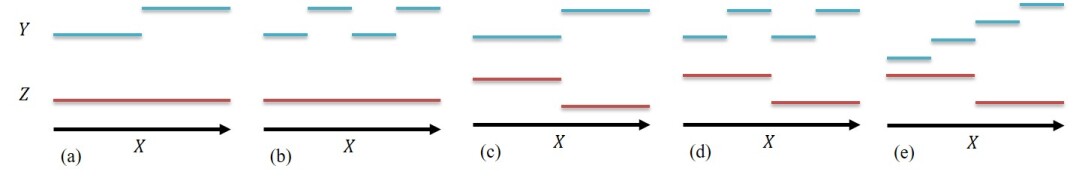
Figure 1: Visualizing toy examples. The transferability between two tasks, represented as sequences $(X,Y)$ and $(X,Z)$. The horizontal axis represent instances and the values for $Z$ (in red) and $Y$ (cyan). In which of these examples would it be easiest to transfer a model trained for task $T^{Z}$ to task $T^{Y}$? See discussion and details in Sec. 3.3.

3.2 The conditional entropy of label sequences

From the label sequences $Y$ and $Z$, we can compute the empirical joint distribution $\hat{P}(y,z)$ for all $(y,z)\in{\mathcal{Y}}\times{\mathcal{Z}}$ by counting, as follows:

$$\hat{P}(y,z)=\frac{1}{n}|\{i:y_{i}=y\text{ and }z_{i}=z\}|.$$ (6)

We now adopt the definition of CE between two random variables [14] to define the CE between our label sequences $Y$ and $Z$.

Definition 2

The CE of a label sequence $Y$ given a label sequence $Z$, $H(Y|Z)$, is the CE of a random variable (or random label) $\bar{y}$ given a random variable (or random label) $\bar{z}$, where $(\bar{y},\bar{z})$ are drawn from the empirical joint distribution $\hat{P}(y,z)$ of Eq. (6):

$$H(Y|Z)=-\sum_{y\in{\mathcal{Y}}}\sum_{z\in{\mathcal{Z}}}\hat{P}(y,z)\log\frac{\hat{P}(y,z)}{\hat{P}(z)},$$ (7)

where $\hat{P}(z)$ is the empirical marginal distribution on ${\mathcal{Z}}$:

$$\hat{P}(z)=\sum_{y\in{\mathcal{Y}}}\hat{P}(y,z)=\frac{1}{n}|\{i:z_{i}=z\}|.$$ (8)

CE represents a measure of the amount of information provided by the value of one random variable on the value of another. By treating the labels assigned to both tasks as random variables and measuring the CE between them, we are measuring the information required to estimate a label in one task given a (known) label in another task.

We now prove a relationship between the CE of Eq. (7) and the tranferability of Eq. (5). In particular, we show that the log-likelihood on the target task $T^{Y}$ is lower bounded by log-likelihood on the source task $T^{Z}$ minus $H(Y|Z)$, if the optimal input representation $w_{Z}$ trained on $T^{Z}$ is transferred to $T^{Y}$.

To prove our theorem, we assume the space $K$ of target classifiers contains a classifier $\bar{k}$ whose log-likelihood lower bounds that of $k_{Y}$. We construct $\bar{k}$ as follows. For each input $x$, we compute the Softmax output $p_{Z}=h_{Z}(w_{Z}(x))$, which is a probability distribution on $\mathcal{Z}$. We then convert $p_{Z}$ into a Softmax on $\mathcal{Y}$ by taking the expectation of the empirical conditional probability ${\hat{P}(y|z)=\hat{P}(y,z)/\hat{P}(z)}$ with respect to $p_{Z}$. That is, for all $y\in\mathcal{Y}$, we define:

$$p_{Y}(y)=\mathbb{E}_{z\sim p_{Z}}[\hat{P}(y|z)]=\sum_{z\in\mathcal{Z}}\hat{P}(y|z)~{}p_{Z}(z),$$ (9)

where $p_{Z}(z)$ is the probability of the label $z$ returned by $p_{Z}$. For any input $w_{Z}(x)$, we let the output of $\bar{k}$ be $p_{Y}$. That is, $\bar{k}(w_{Z}(x))=p_{Y}$. We can now prove the following theorem.

Theorem 1

Under the training procedure described in Sec. 3.1, we have:

$$\widetilde{\mathrm{Trf}}(T^{Z}\rightarrow T^{Y})\geq l_{Z}(w_{Z},h_{Z})-H(Y|Z).$$ (10)

Proof sketch. From the definition of $k_{Y}$ and the assumption that $\bar{k}\in K$, we have $\widetilde{\mathrm{Trf}}(T^{Z}\rightarrow T^{Y})=l_{Y}(w_{Z},k_{Y})\geq l_{Y}(w_{Z},\bar{k})$. From the construction of $\bar{k}$, we have:

$$l_{Y}(w_{Z},\bar{k}) =\frac{1}{n}\sum_{i=1}^{n}\log\left(\sum_{z\in\mathcal{Z}}\hat{P}(y_{i}|z)P(z|x_{i};w_{Z},h_{Z})\right)$$

$${\hskip-46.0pt}\geq\frac{1}{n}\sum_{i=1}^{n}\log\left(\hat{P}(y_{i}|z_{i})P(z_{i}|x_{i};w_{Z},h_{Z})\right)$$ (11)

$${\hskip-46.0pt}=\frac{1}{n}\sum_{i=1}^{n}\log\hat{P}(y_{i}|z_{i})+\frac{1}{n}\sum_{i=1}^{n}\log P(z_{i}|x_{i};w_{Z},h_{Z}).$$ (12)

We can easily show that the first term in Eq. (12) equals $-H(Y|Z)$, while the second term is $l_{Z}(w_{Z},h_{Z})$.

Discussion 1: Generality of our settings. Our settings for spaces $W,H,K$ are general and include a variety of practical use cases. For example, neural networks $W$ will include all possible (vector) values of the network weights until the penultimate layer, while $H$ and $K$ would include all possible (vector) values of the last layer’s weights. Alternatively, we can use support vector machines (SVM) for $K$. In this case, $K$ would include all possible values of the SVM parameters [57]. Our result even holds when the features are fixed, as when using tailored representations such as SIFT [36]. In these cases, space $W$ would contain only one transformation function from raw input to the features.

Discussion 2: Assumptions. We can easily satisfy the assumption $\bar{k}\in K$ by first choosing a space $K^{\prime}$ (e.g., the SVMs) which will play the role of $K\setminus\{\bar{k}\}$. We solve the optimization problem of Eq. (3) on $K^{\prime}$ instead of $K$ to obtain the optimal classifier $k^{\prime}$. To get the optimal classifier $k_{Y}$ on $K=K^{\prime}\cup\{\bar{k}\}$, we simply compare the losses of $k^{\prime}$ and $\bar{k}$ and select the best one as $k_{Y}$.

The optimization problems of Eq. (1) and (3) are global optimization problems. In practice, for complex deep networks trained with stochastic gradient descent, we often only obtain the local optima of the loss. In this case, we can easily change and prove Theorem 1 which would include the differences in the losses between the local optimum and the global optimum in the right-hand-side of Eq. (10). In many practical applications, the difference between local optimum and global optimum is not significant [13, 46].

Discussion 3: Extending our result to test log-likelihood. In Theorem 1, we consider the empirical log-likelihood, which is generally unbounded. If we make the (strong) assumption of bounded differences between empirical log-likelihoods, we can apply McDiarmid’s inequality [42] to get an upper-bound on the left hand side of Eq. (10) by the expected log-likelihood with some probability.

Discussion 4: Implications. Theorem 1 shows that the transferability from task $T^{Z}$ to task $T^{Y}$ depends on both the CE $H(Y|Z)$ and the log-likelihood $l_{Z}(w_{Z},h_{Z})$. Note that the log-likelihood $l_{Z}(w_{Z},h_{Z})$ is optimal for task $T^{Z}$ and so it represents the hardness (or easiness) of task $T^{Z}$. Thus, from the theorem, if $l_{Z}(w_{Z},h_{Z})$ is small (i.e., the source task is hard), transferability would reduce. Besides, if the CE $H(Y|Z)$ is small, transferability would increase.

Finally, we note that when the source task $T^{Z}$ is fixed, the log-likelihood $l_{Z}(w_{Z},h_{Z})$ is a constant. In this case, the transferability only depends on the CE $H(Y|Z)$. Thus, we can estimate the transferability from one source task to multiple target tasks by considering only the CE.

3.3 Intuition and toy examples

To gain intuition on CE and transferability, consider the toy examples illustrated in Fig. 1. The (joint) input set is represented by the $X$ axis. Each input $x_{i}\in X$ is assigned with two labels, $y_{i}\in Y$ and $z_{i}\in Z$, for the two tasks. In Fig. 1(a,b), task $T^{Z}$ is the trivial task with a constant label value (red line) and in Fig. 1(c–e) $T^{Z}$ is a binary classification task, whereas $T^{Y}$ is binary in Fig. 1(a–d) and multi-label in Fig. 1(e). In which of these examples would transferring a representation trained for $T^{Z}$ to $T^{Y}$ be hardest?

Of the five examples, (c) is the easiest transfer as it provides a 1-1 mapping from $Z$ to $Y$. Appropriately, in this case, $H(Y|Z)=0$. Next up are (d) and (e) with $H(Y|Z)=\log 2$: In both cases each class in $T^{Z}$ is mapped to two classes in $T^{Y}$. Note that $T^{Y}$ being non-binary is naturally handled by the CE. Finally, transfers (a) and (b) have $H(Y|Z)=4\log 2$; the highest CE. Because $T^{Z}$ is trivial, the transfer must account for the greatest difference in the information between the tasks and so the transfer is hardest.

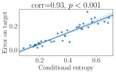
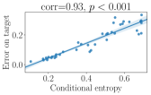
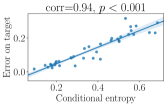
(a) Heavy makeup	(b) Male	(c) Pale skin	(d) Wearing lipstick
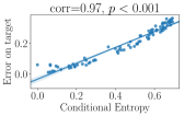
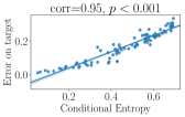
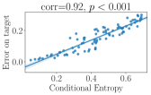
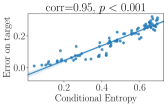
(e) Swim	(f) Pads	(g) Paws	(h) Strong
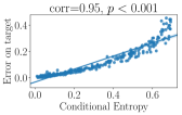
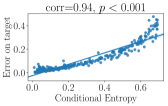
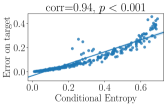
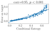
(i) Curved Bill	(j) Iridescent Wings	(k) Brown Upper Parts	(l) Olive Under Parts

Figure 2: Attribute prediction; CE vs. test errors on target tasks. Examples from CelebA (a-d), AwA2 (e-h), and CUB (i-l). Plot titles name the source tasks $T^{Z}$; points represent different target tasks $T^{Y}$. Corr is the Pearson correlation coefficient between the two variables and $p$ is the statistical significance of the correlation. In all cases, the correlation is statistically significant. See Sec. 5.1 for details.

	Attribute:	Male	Bald	Gray Hair	Mustache	Double Chin	$\ldots$	Attractive	Wavy Hair	High Cheeks	Smiling	Mouth Open	Average (all)
1	LNets+ANet 2015  [35]	0.980	0.980	0.970	0.950	0.920	$\ldots$	0.810	0.800	0.870	0.920	0.920	0.873
2	Walk and Learn 2016 [63]	0.960	0.920	0.950	0.900	0.930		0.840	0.850	0.950	0.980	0.970	0.887
3	MOON 2016 [55]	0.981	0.988	0.981	0.968	0.963		0.817	0.825	0.870	0.926	0.935	0.909
4	LMLE 2016 [26]	0.990	0.900	0.910	0.730	0.740		0.880	0.830	0.920	0.990	0.960	0.838
5	CR-I 2017 [16]	0.960	0.970	0.950	0.940	0.890		0.830	0.790	0.890	0.930	0.950	0.866
6	MCNN-AUX 2017 [23]	0.982	0.989	0.982	0.969	0.963		0.831	0.839	0.876	0.927	0.937	0.913
7	DMTL 2018 [22]	0.980	0.990	0.960	0.970	0.990		0.850	0.870	0.880	0.940	0.940	0.926
8	Face-SSD 2019 [27]	0.973	0.986	0.976	0.960	0.960		0.813	0.851	0.868	0.918	0.919	0.903
lightblue9	CE$\uparrow$ (decreasing transferability)	0.017	0.026	0.052	0.062	0.083		0.361	0.381	0.476	0.521	0.551	-
10	Dedicated Res18	0.985	0.990	0.980	0.968	0.959		0.823	0.842	0.878	0.933	0.943	0.911
11	Transfer	0.992	0.991	0.981	0.968	0.963		0.820	0.800	0.859	0.909	0.901	0.902

Table 1: Transferability from face recognition to facial attributes. Results for CelebA attributes, sorted in ascending order of row 9 (decreasing transferability). Results are shown for the five attributes most and least transferable from recognition. Subject specific attributes, e.g., male and bald, are more transferable than expression related attributes such as smiling and mouth open. Unsurprisingly, transfer results (row 11) are best on the former than the latter. Rows 1-8 provide published state of the art results. Despite training only an lSVM for attribute, row 11 results are comparable with more elaborate attribute classification systems. For details, see Sec. 5.2.

4 Task hardness

A potential application of transferability is task hardness. In Sec. 3.2, we mentioned that the hardness of a task can be measured from the optimal log-likelihood on that task. Formally, we can measure the hardness of a task $T^{Z}$ by:

$$\mathrm{Hard}(T^{Z})=\min_{w,h\in(W,H)}\mathcal{L}_{Z}(w,h)=-l_{Z}(w_{Z},h_{Z}).$$ (13)

This definition of hardness depends on our choice of $(W,H)$, which may determine various factors such as representation size or network architecture. The intuition behind the definition is that if the task $T^{Z}$ is hard for all models in $(W,H)$, we should expect higher loss even after training.

Using Theorem 1, we can bound $l_{Z}(w_{Z},h_{Z})$ in Eq. (13) by transferring from a trivial task $T^{C}$ to $T^{Z}$. We define a trivial task as the task for which all input values are assigned the same, constant label. Let $C$ be the (constant) label sequences of the trivial task $T^{C}$. From Theorem 1 and Eq. (13), we can easily show that:

$$\mathrm{Hard}(T^{Z})=-l_{Z}(w_{Z},h_{Z})\leq H(Z|C).$$ (14)

Thus, we can approximate the hardness of task $T^{Z}$ by looking at the CE $H(Z|C)$. We note that the CE $H(Z|C)$ is also used to estimate the transferability ${\widetilde{\mathrm{Trf}}(T^{C}\rightarrow T^{Z})}$. So, $\mathrm{Hard}(T^{Z})$ is closely related to ${\widetilde{\mathrm{Trf}}(T^{C}\rightarrow T^{Z})}$. Particularly, if task $T^{Z}$ is hard, we expect it is more difficult to transfer from a trivial task to $T^{Z}$.

This relationship between hardness and transferability from a trivial task is similar to the one proposed by Task2Vec [1]. They too indexed task hardness as the distance from a trivial task. To compute task hardness, however, they required training deep models, whereas we obtain this measure by simply computing $H(Z|C)$ using Eq. (7).

Of course, estimating the hardness by $H(Z|C)$ ignores the input and is hence only an approximation. In particular, one could possibly design scenarios where this measure would not accurately reflect the hardness of a given task. Our results in Sec. 5.3 show, however, that these label statistics provide a strong cue for task hardness.

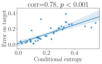
Figure 3: Identity to attribute; CE vs. test errors on target tasks. Predicting 40 CelebA attributes using a face recognition network. Corr is the Pearson correlation coefficient between the two variables, and $p$ is the statistical significance of the correlation.

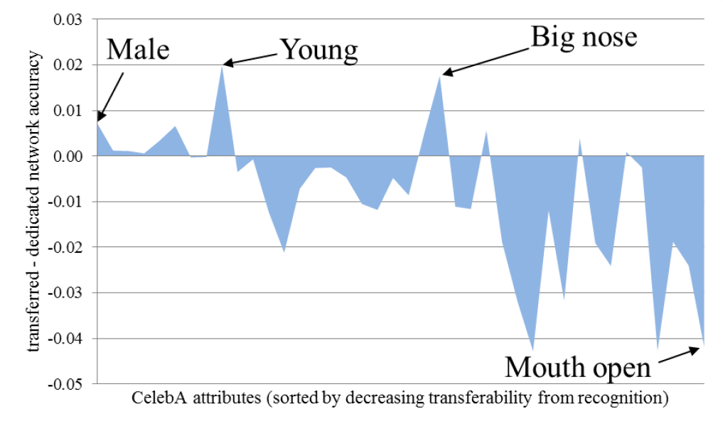
Figure 4: Identity to attribute; transferred $-$ dedicated accuracy. Differences between CelebA accuracy of transferred recognition model and models trained for each attribute. Results are sorted by decreasing transferability (same as Table 1).

5 Experiments

We rigorously evaluate our claims using three large scale, widely used data sets representing 437 classification tasks. Although Sec. 3.2 provides a bound on the training loss, test accuracy is generally more important. We thus report results on test images not included in the training data.

Benchmarks. The Celeb Faces Attributes (CelebA) set [35] was extensively used to evaluate transfer learning [18, 33, 34, 58]. CelebA contains over 202k face images of 10,177 subjects. Each image is labeled with subject identity as well as 40 binary attributes. We used the standard train / test splits (182,626 / 19,961 images, respectively). To our knowledge, of the three sets, it is the only one that provides baseline results for attribute classification.

Animals with Attributes 2 (AwA2) [67] includes over 37k images labeled as belonging to one of 50 animals classes. Images are labeled based on their class association with 85 different attributes. Models were trained on 33,568 training images and tested on 3,754 separate test images.

Finally, Caltech-UCSD Birds 200 (CUB) [66] offers 11,788 images of 200 bird species, labeled with 312 attributes as well as Turker Confidence attributes. Labels were averaged across multiple Turkers using confidences. Finally, we kept only reliable labels, using a threshold of 0.5 on the average confidence value. We used 5,994 images for training and 5,794 images for testing.

We note that the Task Bank set with its 26 tasks was also used for evaluating task relationships [71]. We did not use it here as it mostly contains regression tasks rather than the classification problems we are concerned with.

5.1 Evaluating task transferability

We compared our transferability estimates from the CE to the actual transferability of Eq. (4). To this end, for each attribute $T^{Z}$ in a data set, we measure the actual transferability, $\mathrm{Trf}(T^{Z}\rightarrow T^{Y})$, to all other attributes $T^{Y}$ in that set using the test split. We then compare these transferability scores to the corresponding CE estimates of Eq. (7) using an existing correlation analysis [44].

We note again that when the source task is fixed, as in this case, the transferability estimates can be obtained by considering only the CE. Furthermore, since $\mathrm{Trf}(T^{Z}\rightarrow T^{Y})$ and the CE $H(Y|Z)$ are negative correlated, we compare the correlation between the test error rate, $1-\mathrm{Trf}(T^{Z}\rightarrow T^{Y})$, and the CE $H(Y|Z)$ instead.

Transferring representations. We keep the learned representation, $w_{Z}$, and produce a new classifier $k_{Y}$ by training on the target task (Sec. 3.1). We used ResNet18 [25], trained with standard cross entropy loss, on each source task $T^{Z}$ (source attribute). These networks were selected as they were deep enough to obtain good accuracy on our benchmarks, but not too deep to overfit [72]. The penultimate layer of these networks produce embeddings $r\in\mathbb{R}^{2048}$ which the networks classified using $h_{Z}$—their last, fully connected (FC) layers—to binary attribute values.

We transferred from source to target task by freezing the networks, only replacing their FC layers with linear SVM (lSVM). These lSVM were trained to predict the binary labels of target tasks given the embeddings produced for the source tasks by $w_{Z}$ as their input. The test errors of the lSVM, which are measures of ${1-\mathrm{Trf}(T^{Z}\rightarrow T^{Y})}$, were then compared with the CE, $H(Y|Z)$.

We use lSVM as it allows us to focus on the information passed from $T^{Z}$ to $T^{Y}$. A more complex classifier could potentially mask this information by being powerful enough to offset any loss of information due to the transfer. In practical use cases, when transferring a deep network from one task to another, it may be preferable to fine tune the last layers of the network or its entirety, provided that the training data on the target task is large enough.

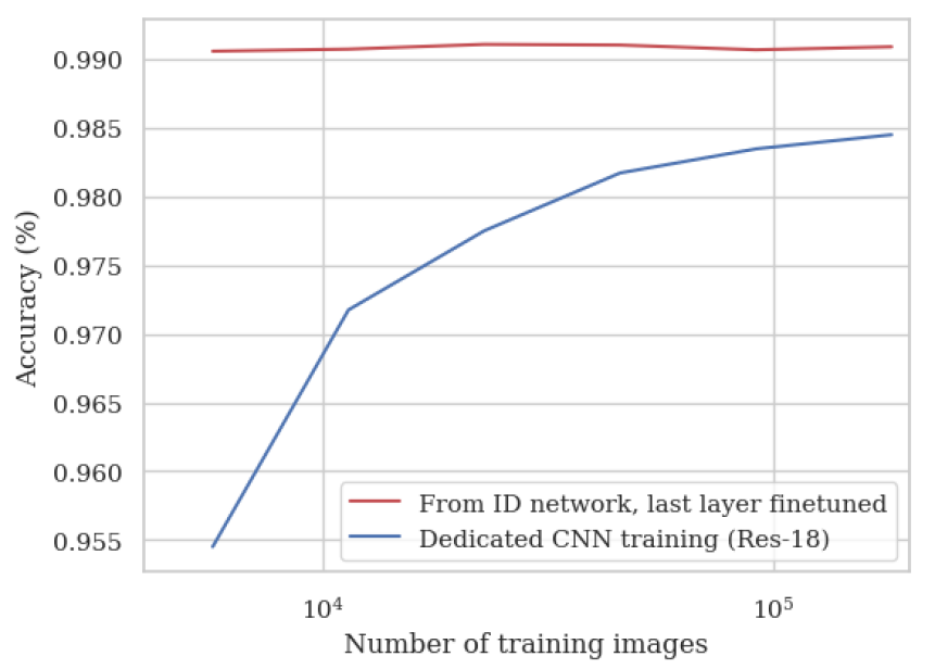
(a) Male

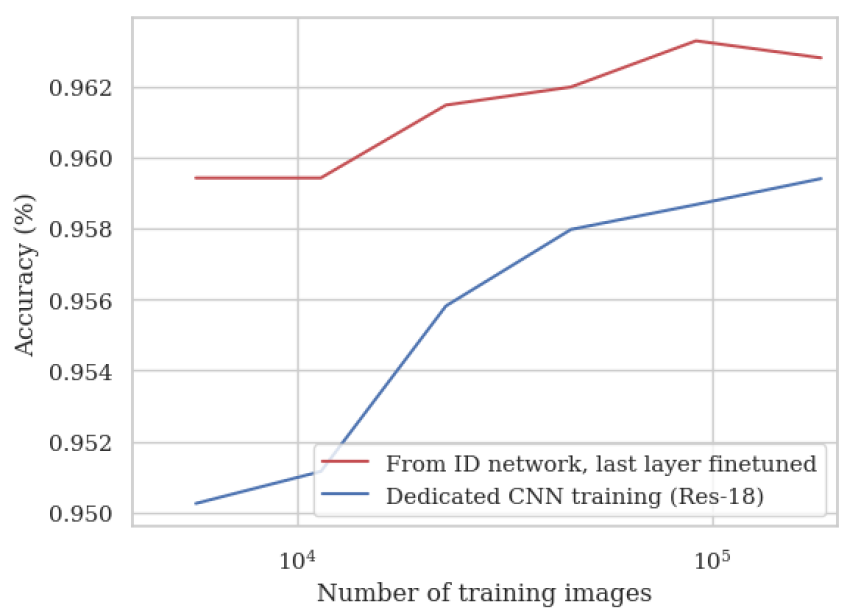
(b) Double chin

Figure 5: Classification accuracy for varying training set sizes. Top: male; bottom: double chin. Dedicated classification networks trained from scratch (blue) vs. face recognition network transferred to the attributes with an lSVM (red). Because recognition transfers well to these attributes, we obtain accurate classification with a fraction of the training data and effort.

Transferability results. Fig. 2 reports selected quantitative transferability results on the three sets. Each point in these graphs represents the CE, $H(Y|Z)$, vs. the target test error, ${1-\mathrm{Trf}(T^{Z}\rightarrow T^{Y})}$. The graphs also provide the linear regression model fit with 95% confidence interval, the Pearson correlation coefficients between the two values, and the statistical significance of the correlation, $p$.

In all cases, the CE and target test error are highly positively correlated with statistical significance. These results testify that the CE of Eq. (7) is indeed a good predictor for the actual transferability of Eq. (4). This is remarkable especially since the relationship between tasks is evaluated without considering the input domain or the machine learning models trained to solve these tasks.

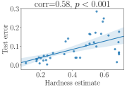
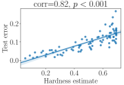
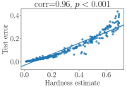
(a) CelebA	(b) AwA2	(c) CUB

Figure 6: Estimated task hardness vs. empirical errors on the three benchmarks. Estimated hardness is well correlated with empirical hardness with significance $p<0.001$.

5.2 Case study: Identity to facial attributes

A key challenge when training effective attribute classifiers is the difficulty of obtaining labeled attribute training data. Whereas face images are often uploaded to the Internet along with subject names [9, 21], it is far less common to find images labeled with attributes such as high cheek bones, bald, or even male [32]. It is consequently harder to assemble training sets for attribute classification at the same scale and diversity as those used to train other tasks.

To reduce the burden of collecting attribute data, we therefore explore transferring a representation learned for face recognition. In this setting, we can also compute estimated transferability scores (via the CE) between the subject labels provided by CelebA and the labels of each attribute. We note that unlike the previous examples, the source labels are not binary and include over 10k values.

Face recognition network. We compare our estimated transferability vs. actual transferability using a deep face recognition network. To this end, we use a ResNet101 architecture trained for face recognition on the union of the MS-Celeb-1M [21] and VGGFace2 [9] training sets (following removal of subjects included in CelebA), with a cosine margin loss ($m=0.4$) [62]. This network achieves accuracy comparable to the state of the art reported by others, with different systems, on standard benchmarks [15].

Transferability results: recognition to attributes. Table 1 reports results for the five attributes most transferable from recognition (smallest CE; Eq. (7)) and the five least transferable (largest CE). Columns are sorted by increasing CE values (decreasing transferability), listed in row 9. Row 11 reports accuracy of the transferred network with the lSVM trained on the target task. Estimated vs. actual transferability is further visualized in Fig. 3. Evidently, correlation between the two is statistically significant, testifying that Eq. (7) is a good predictor of actual transferability, here demonstrated on a source task with multiple labels.

For reference, Table 1 provides in Row 10 the accuracy of the dedicated ResNet18 networks trained for each attribute. Finally, rows 1 through 8 provide results for published state of the art on the same tasks.

Analysis of results. Subject specific attributes such as male and bald are evidently more transferable from recognition (left columns of Table 1) than attributes that are related to expressions (e.g., smiling and mouth open, right columns). Although this relationship has been noted by others, previous work used domain knowledge to determine which attributes are more transferable from identity [35], as others have done in other domains [20, 38]. By comparison, our work shows how these relationships emerge from our estimation of transferability.

Also, notice that for the transferable attributes, our results are comparable to dedicated networks trained for each attribute, although they gradually drop off for the less transferable attributes in the last columns. This effect is visualized in Fig. 4 which shows the growing differences in attribute classification accuracy for a transferred face recognition model and models trained for each attribute. Results are sorted by decreasing transferability (same as in Table 1).

Results in Fig. 4 show a few notable exceptions where transfer performs substantially better than dedicated models (e.g., the two positive peaks representing attributes young and big nose). These and other occasional discrepancies in our results can be explained in the difference between the true transferability of Eq. (4), which we measure on the test sets, and Eq. (5), defined on the training sets and shown in Sec. 3.2 to be bounded by the CE.

Finally, we note that our goal is not to develop a state of the art facial attribute classification scheme. Nevertheless, results obtained by training an lSVM on embeddings transferred from a face recognition network are only 2.4% lower than the best scores reported by DMTL 2018 [22] (last column of Table 1). The effort involved in developing a state of the art face recognition network can be substantial. By transferring this network to attributes these efforts are amortized in training multiple facial attribute classifiers.

To emphasize this last point, consider Fig. 5 which reports classification accuracy on male and double chin for growing training set sizes. These attributes were selected as they are highly transferable from recognition (see Table 1). The figure compares the accuracy obtained by training a dedicated network (in blue) to a network transferred from recognition (red). Evidently, on these attributes, transferred accuracy is much higher with far less training data.

5.3 Evaluating task hardness

We evaluate our hardness estimates for all attribute classification tasks in the three data sets, using the CE $H(Z|C)$ in Eq. (14). Fig. 6 compares the hardness estimates for each task vs. the errors of our dedicated networks, trained from scratch to classify each attribute. Results are provided for CelebA, AwA2, and CUB.

The correlation between estimated hardness and classification errors is statistically significant with $p<0.001$, suggesting that the CE $H(Z|C)$ in Eq. (14) indeed captures the hardness of these tasks. That is, in the three data sets, test error rates strongly correlate with our estimated hardness: the harder a task is estimated to be, the higher the errors produced by the model trained for the task. Of course, this result does not imply that the input domain has no impact on task hardness; only that the distribution of training labels already provides a strong predictor for task hardness.

6 Conclusions

We present a practical method for estimating the hardness and transferability of supervised classification tasks. We show that, in both cases, we produce reliable estimates by exploring training label statistics, particularly the conditional entropy between the sequences of labels assigned to the training data of each task. This approach is simpler than existing work, which obtains similar estimates by assuming the existence of trained models or by careful inspection of the training process. In our approach, computing conditional entropy is cheaper than training deep models, required by others for the same purpose.

We assume that different tasks share the same input domain (the same input images). It would be useful to extend our work to settings where the two tasks are defined over different domains (e.g., face vs. animal images). Our work further assumes discrete labels. Conditional entropy was originally defined over distributions. It is therefore reasonable that CE could be extended to non-discrete labeled tasks, such as, for faces, 3D reconstruction [60], pose estimation [10, 11] or segmentation [47].

Acknowledgements. We thank Alessandro Achille, Pietro Perona, and the reviewers for their helpful discussions.

Appendix A Proof of theorem 1

From the definition of $\widetilde{\mathrm{Trf}}(T^{Z}\rightarrow T^{Y})$, we have:

$$\widetilde{\mathrm{Trf}}(T^{Z}\rightarrow T^{Y})$$

$$=l_{Y}(w_{Z},k_{Y}) \widetilde{\mathrm{Trf}}$$ (definition of )

$$\geq l_{Y}(w_{Z},\bar{k}) k_{Y} \bar{k}\in K$$ (definition of and )

$$=\frac{1}{n}\sum_{i=1}^{n}\log\left(\sum_{z\in\mathcal{Z}}\hat{P}(y_{i}|z)P(z|x_{i};w_{Z},h_{Z})\right) \bar{k}$$ (construction of )

$$\geq\frac{1}{n}\sum_{i=1}^{n}\log\left(\hat{P}(y_{i}|z_{i})P(z_{i}|x_{i};w_{Z},h_{Z})\right)$$ (replacing the sum by one of its elements)

$$=\frac{1}{n}\sum_{i=1}^{n}\log\hat{P}(y_{i}|z_{i})+\frac{1}{n}\sum_{i=1}^{n}\log P(z_{i}|x_{i};w_{Z},h_{Z}).$$ (15)

Note that the second term in Eq. (15) is:

$$\frac{1}{n}\sum_{i=1}^{n}\log P(z_{i}|x_{i};w_{Z},h_{Z})=l_{Z}(w_{Z},h_{Z}).$$ (16)

Furthermore, the first term in Eq. (15) is:

$$\frac{1}{n}\sum_{i=1}^{n}\log\hat{P}(y_{i}|z_{i})$$

$$=\frac{1}{n}\sum_{y\in\mathcal{Y}}\sum_{z\in\mathcal{Z}}\left(\sum_{i~{}:~{}y_{i}=y\text{ and }z_{i}=z}\log\hat{P}(y|z)\right) y_{i} z_{i}$$ (group the summands by values of and )

$$=\frac{1}{n}\sum_{y\in\mathcal{Y}}\sum_{z\in\mathcal{Z}}\left(\left|\left\{i:y_{i}=y\text{ and }z_{i}=z\right\}\right|~{}\log\hat{P}(y|z)\right)$$ (by counting)

$$=\sum_{y\in\mathcal{Y}}\sum_{z\in\mathcal{Z}}\left(\frac{\left|\left\{i:y_{i}=y\text{ and }z_{i}=z\right\}\right|}{n}~{}\log\hat{P}(y|z)\right)$$

$$=\sum_{y\in\mathcal{Y}}\sum_{z\in\mathcal{Z}}\left(\hat{P}(y,z)~{}\log\frac{\hat{P}(y,z)}{\hat{P}(z)}\right) \hat{P}(y,z) \hat{P}(y|z)$$ (definitions of and )

$$=-H(Y|Z).$$ (17)

From Eq. (15), (16), and (17), we have ${\widetilde{\mathrm{Trf}}(T^{Z}\rightarrow T^{Y})}\geq l_{Z}(w_{Z},h_{Z})-H(Y|Z)$. Hence, the theorem holds.

Appendix B More details on task hardness

On the definition of task hardness. In our paper, we assume non-overfitting of trained models. When train and test sets are sampled from the same distribution, this assumption typically holds for appropriately trained models [72]. This property also shows that our definition of hardness, Eq. (13), does not conflict with the results of Zhang et al. [72]: In such cases, the training loss of Eq. (13) correlates with the test error, and thus this definition indeed reflects task hardness, explaining the relationships between train and test errors observed in our hardness results.

On the representation for trivial tasks. Any representation for a trivial source task can fit the constant label perfectly (zero training loss). In theory, if we choose the optimal $w_{Z}$ in Eq. (1) as our representation, we can show Eq. (14). In practice, of course we cannot infer the optimal $w_{Z}$ from the trivial source task, but Eq. (14) shows that we can still connect it to $H(Z|C)$.

Appendix C Technical implementation details

Computing the CE. Computing the CE is straightforward and involves the following steps:

1. Loop through the training labels of both tasks $T^{Z}$ and $T^{Y}$ and compute the empirical joint distribution $\hat{P}(y,z)$ by counting (Eq. (6) in the paper).

2. Loop through the training labels again and compute the CE using Eq. (17) above. That is,

   $$H(Y|Z)=-\frac{1}{n}\sum_{i=1}^{n}\log\hat{P}(y_{i}|z_{i}).$$

Thus, computing the CE only requires running two loops through the training labels. This process is computationally efficient. In the most extreme case, computing the transferability of face recognition ($|\mathcal{Z}|>10k$) to a facial attribute, with $|\mathcal{Y}|=2$, required less than a second on a standard CPU.

This run time should be compared with the hours (or days) required to train deep models in order to empirically measure transferability following the process described by previous work. In particular, Taskonomy [71] reported over 47 thousand hours of GPU runtime in order to establish relationships between their 26 tasks.

Dedicated attribute training. Given a source task $T^{Z}$, we train a dedicated CNN for this task with standard ResNet-18 V2 implemented in the MXNet deep learning library [12]. We set the initial learning rate to 0.01. Learning rate was then divided by 10 after each 12 epochs. Training converged in less than 40 epochs in all 437 tasks.

Task transfer with linear SVM. After training a deep representation for a source task $T^{Z}$, we transfer it to a target task $T^{Y}$ using linear support vector machines (lSVM).

First, we use the trained CNN, denoted in the paper as $w_{Z}$, to extract deep embeddings for the entire training data (one embedding per input image. Each embedding is a vector $r\in\mathbb{R}^{2048}$, which we obtain from the penultimate layer of the network. We then use these embeddings, along with the corresponding labels for target task, $T^{Y}$, to train a standard lSVM classifier, implemented by SK-Learn [49]. The lSVM parameters were kept unchanged from their default values.

Given unseen testing data, we first extract their embeddings with $w_{Z}$. We then apply the trained lSVM classifier on these features to predict labels for target task, $T^{Y}$.

Appendix D Additional results: Generalization to multi-class

Transferability generalizes well to multi-class, as evident in our face recognition (10k labels)-to-attribute tests in Sec. 5.2. Table 2 below reports hardness tests with multi-class, CelebA, attribute aggregates. Generally speaking, the harder the task, the lower the accuracy obtained.

Multi-class	Straight/Wavy/Other	Black/Blonde/Other	Arched/Bushy/Other
lightblue Hardness $\downarrow$	1.040	0.925	0.867
Dedicated Res18	0.713	0.859	0.797
Multi-class	Bangs/Receding/Other	Gray/Blonde/Other	Goatee/Beard/None
lightblue Hardness $\downarrow$	0.690	0.575	0.557
Dedicated Res18	0.900	0.943	0.937

Table 2: Multi-class hardness examples on CelebA data.

Appendix E Full transferability results

• Attribute prediction on CelebA [35]: see Fig. 7.

• CelebA: Transferability from identity to attributes: see Table 3.

• Attribute prediction on AwA2 [67]: see Fig. 8, 9, and 10.

(0) 5 o’clock shadow	(1) Arched eyebrows	(2) Attractive	(3) Bags under eyes	(4) Bald
(5) Bangs	(6) Big lips	(7) Big nose	(8) Black hair	(9) Blond hair
(10) Blurry	(11) Brown hair	(12) Bushy eyebrows	(13) Chubby	(14) Double chin
(15) Eyeglasses	(16) Goatee	(17) Gray hair	(18) Heavy makeup	(19) High cheekbones
(20) Male	(21) Mouth slightly open	(22) Mustache	(23) Narrow eyes	(24) No Beard
(25) Oval face	(26) Pale skin	(27) Pointy nose	(28) Receding hairline	(29) Rosy cheeks
(30) Sideburns	(31) Smiling	(32) Straight hair	(33) Wavy hair	(34) Wearing earrings
(35) Wearing hat	(36) Wearing lipstick	(37) Wearing necklace	(38) Wearing necktie	(39) Young

Figure 7: Attribute prediction; CE vs. test errors on CelebA (Extended from Fig. 2(a-d) in the paper). The source attribute, $T^{Z}$, in each plot is named in the plot title. Points represent different target tasks $T^{Y}$. Corr is the Pearson correlation coefficient between the two variables and $p$ is the statistical significance of the correlation. In all cases, the correlation is statistically significant.

	Attribute:	Male	Bald	Gray Hair	Mustache	Double Chin	Chubby	Sideburns	Goatee	Young	Wear Hat	$\rightarrow$
1	LNets$+$ANet 2015  [35]	0.980	0.980	0.970	0.950	0.920	0.910	0.960	0.950	0.870	0.990
2	Walk and Learn 2016 [63]	0.960	0.920	0.950	0.900	0.930	0.890	0.920	0.920	0.860	0.960
3	MOON 2016 [55]	0.981	0.988	0.981	0.968	0.963	0.954	0.976	0.970	0.881	0.990
4	LMLE 2016 [26]	0.990	0.900	0.910	0.730	0.740	0.790	0.880	0.950	0.870	0.990
5	CR-I 2017 [16]	0.960	0.970	0.950	0.940	0.890	0.870	0.920	0.960	0.840	0.980
6	MCNN-AUX 2017 [23]	0.982	0.989	0.982	0.969	0.963	0.957	0.978	0.972	0.885	0.990
7	DMTL 2018 [22]	0.980	0.990	0.960	0.970	0.990	0.970	0.980	0.980	0.900	0.990
8	Face-SSD 2019 [27]	0.973	0.986	0.976	0.960	0.960	0.951	0.966	0.963	0.876	0.985
lightblue9	Conditional Entropy$\uparrow$	0.017	0.026	0.052	0.062	0.083	0.087	0.088	0.089	0.095	0.107
10	Dedicated Res18	0.985	0.990	0.980	0.968	0.959	0.951	0.976	0.974	0.879	0.991
11	FromID SVM	0.992	0.991	0.981	0.968	0.963	0.957	0.976	0.973	0.899	0.988
	Attribute:	Eye glasses	Pale Skin	Wear Necktie	Blurry	No Beard	Receding Hairline	5 clock Shadow	Rosy Cheeks	Blond Hair	Big Lips	$\rightarrow$
1		0.990	0.910	0.930	0.840	0.950	0.890	0.910	0.900	0.950	0.680
2		0.970	0.850	0.840	0.910	0.900	0.840	0.840	0.960	0.920	0.780
3		0.995	0.970	0.966	0.957	0.956	0.936	0.940	0.948	0.959	0.715
4		0.980	0.800	0.900	0.590	0.960	0.760	0.820	0.780	0.990	0.600
5		0.960	0.920	0.880	0.850	0.940	0.870	0.900	0.880	0.950	0.680
6		0.996	0.970	0.965	0.962	0.960	0.938	0.945	0.952	0.960	0.715
7		0.990	0.970	0.970	0.960	0.970	0.940	0.950	0.960	0.910	0.880
8		0.992	0.957	0.956	0.950	0.949	0.931	0.929	0.943	0.936	0.778
lightblue9		0.109	0.122	0.131	0.139	0.141	0.141	0.145	0.152	0.16	0.161
10		0.997	0.970	0.963	0.963	0.961	0.936	0.942	0.950	0.961	0.715
11		0.996	0.958	0.941	0.956	0.958	0.933	0.937	0.939	0.949	0.710
	Attribute:	Bushy Eyebrows	Wear Lipstick	Big Nose	Bangs	Narrow Eyes	Wear Necklace	Heavy Makeup	Black Hair	Wear Earrings	Arched Eyebrows	$\rightarrow$
1		0.900	0.930	0.780	0.950	0.810	0.710	0.900	0.880	0.820	0.790
2		0.930	0.920	0.910	0.960	0.790	0.770	0.960	0.840	0.910	0.870
3		0.926	0.939	0.840	0.958	0.865	0.870	0.910	0.894	0.896	0.823
4		0.820	0.990	0.800	0.980	0.590	0.590	0.980	0.920	0.830	0.790
5		0.840	0.940	0.800	0.950	0.720	0.740	0.840	0.900	0.830	0.800
6		0.928	0.941	0.845	0.960	0.872	0.866	0.915	0.898	0.904	0.834
7		0.850	0.930	0.920	0.960	0.900	0.890	0.920	0.850	0.910	0.860
8		0.896	0.926	0.823	0.952	0.890	0.878	0.907	0.879	0.869	0.820
lightblue9		0.192	0.202	0.232	0.236	0.252	0.252	0.27	0.286	0.291	0.306
10		0.927	0.935	0.828	0.961	0.875	0.859	0.916	0.901	0.896	0.834
11		0.919	0.940	0.845	0.950	0.863	0.865	0.897	0.869	0.853	0.822
	Attribute:	Brown Hair	Bags U Eyes	Oval Face	Straight Hair	Pointy Nose	Attractive	Wavy Hair	High Cheeks	Smiling	Mouth Open	Average (all)
1		0.800	0.790	0.660	0.730	0.720	0.810	0.800	0.870	0.920	0.920	0.873
2		0.810	0.870	0.790	0.750	0.770	0.840	0.850	0.950	0.980	0.970	0.887
3		0.894	0.849	0.757	0.823	0.765	0.817	0.825	0.870	0.926	0.935	0.909
4		0.870	0.730	0.680	0.730	0.720	0.880	0.830	0.920	0.990	0.960	0.838
5		0.860	0.800	0.660	0.730	0.730	0.830	0.790	0.890	0.930	0.950	0.866
6		0.892	0.849	0.758	0.836	0.775	0.831	0.839	0.876	0.927	0.937	0.913
7		0.960	0.990	0.780	0.850	0.780	0.850	0.870	0.880	0.940	0.940	0.926
8		0.835	0.825	0.748	0.834	0.749	0.813	0.851	0.868	0.918	0.919	0.903
lightblue9		0.315	0.324	0.339	0.339	0.341	0.361	0.381	0.476	0.521	0.551
10		0.886	0.834	0.752	0.836	0.769	0.823	0.842	0.878	0.933	0.943	0.911
11		0.854	0.838	0.733	0.812	0.769	0.820	0.800	0.859	0.909	0.901	0.902

Table 3: Transferability from face recognition to facial attributes. (Extended from Table 1 in the paper) Results for CelebA attributes, sorted in ascending order of row 9 (decreasing transferability). Classification accuracies are shown for all 40 attributes. Subject specific attributes, e.g., male and bald, are more transferable than expression related attributes such as smiling and mouth open. These identity specific attributes corresponds to the automatic grouping presented in the original CelebA paper [35]. Unlike them, however, we obtain this grouping without necessitating the training of a deep attribute classification model. Unsurprisingly, transfer results (row 11) are best on these subject specific attributes and worst for less related attributes. Rows 1-8 provide published state of the art results. Despite training only an lSVM for attribute, row 11 results are comparable with more elaborate attribute classification systems. For details, see Sec. 5.2.

(0) Black	(1) White	(2) Blue	(3) Brown	(4) Gray
(5) Orange	(6) Red	(7) Yellow	(8) Patches	(9) Spots
(10) Stripes	(11) Furry	(12) Hairless	(13) Toughskin	(14) Big
(15) Small	(16) Bulbous	(17) Lean	(18) Flippers	(19) Hands
(20) Hooves	(21) Pads	(22) Paws	(23) Longleg	(24) Longneck
(25) Tail	(26) Chewteeth	(27) Meatteeth	(28) Buckteeth	(29) Strainteeth
(30) Horns	(31) Claws	(32) Tusks	(33) Smelly	(34) Flys

Figure 8: Attribute prediction; CE vs. test errors on AwA2 (Extended from Fig. 2(e-h) in the paper; part 1). The source attribute, $T^{Z}$, in each plot is named in the plot title. Points represent different target tasks $T^{Y}$. Corr is the Pearson correlation coefficient between the two variables and $p$ is the statistical significance of the correlation. In all cases, the correlation is statistically significant.

(35) Hops	(36) Swims	(37) Tunnels	(38) Walks	(39) Fast
(40) Slow	(41) Strong	(42) Weak	(43) Muscle	(44) Bipedal
(45) Quadrapedal	(46) Active	(47) Inactive	(48) Nocturnal	(49) Hibernate
(50) Agility	(51) Fish	(52) Meat	(53) Plankton	(54) Vegetation
(55) Insects	(56) Forager	(57) Grazer	(58) Hunter	(59) Scavenger
(60) Skimmer	(61) Stalker	(62) Newworld	(63) Oldworld	(64) Arctic
(65) Coastal	(66) Desert	(67) Bush	(68) Plains	(69) Forest

Figure 9: Attribute prediction; CE vs. test errors on AwA2 (Extended from Fig. 2(e-h) in the paper; part 2). The source attribute, $T^{Z}$, in each plot is named in the plot title. Points represent different target tasks $T^{Y}$. Corr is the Pearson correlation coefficient between the two variables and $p$ is the statistical significance of the correlation. In all cases, the correlation is statistically significant.

(70) Fields	(71) Jungle	(72) Mountains	(73) Ocean	(74) Ground
(75) Water	(76) Tree	(77) Cave	(78) Fierce	(79) Timid
(80) Smart	(81) Group	(82) Solitary	(83) Nestspot	(84) Domestic

Figure 10: Attribute prediction; CE vs. test errors on AwA2 (Extended from Fig. 2(e-h) in the paper; part 3). The source attribute, $T^{Z}$, in each plot is named in the plot title. Points represent different target tasks $T^{Y}$. Corr is the Pearson correlation coefficient between the two variables and $p$ is the statistical significance of the correlation. In all cases, the correlation is statistically significant.

Appendix F Full hardness results

• CelebA [35] attribute prediction hardness: see Table 4.

• AwA2 [67] attribute prediction hardness: see Table 5.

• CUB [66] attribute prediction hardness: see Table 6.

1	Attribute	Bald	Mustache	Gray Hair	Pale Skin	Double Chin	Wearing Hat	Blurry	Sideburns	Chubby	Goatee	$\rightarrow$
lightblue2	Conditional Entropy$\uparrow$	0.107	0.173	0.174	0.177	0.189	0.194	0.201	0.217	0.22	0.235	$\rightarrow$
	$\rightarrow$	Eyeglasses	Rosy Cheeks	Wearing Necktie	Receding Hairline	5 oClock Shadow	Narrow Eyes	Wearing Necklace	Bushy Eyebrows	Blond Hair	Bangs	$\rightarrow$
lightblue	$\rightarrow$	0.241	0.242	0.261	0.278	0.349	0.357	0.373	0.409	0.419	0.425	$\rightarrow$
	$\rightarrow$	No Beard	Wearing Earrings	Bags Under Eyes	Brown Hair	Straight Hair	Young	Big Nose	Black Hair	Big Lips	Arched Eyebrows	$\rightarrow$
lightblue	$\rightarrow$	0.448	0.485	0.507	0.508	0.512	0.535	0.545	0.55	0.552	0.58	$\rightarrow$
	$\rightarrow$	Pointy Nose	Oval Face	Wavy Hair	Heavy Makeup	Male	High Cheekbones	Wearing Lipstick	Smiling	Mouth Slightly Open	Attractive
lightblue	$\rightarrow$	0.591	0.597	0.627	0.667	0.679	0.689	0.692	0.693	0.693	0.693

Table 4: CelebA task hardness. CelebA facial attributes sorted in ascending order of hardness along with their respective hardness scores. Hardness scores listed above are compared with empirical test errors for each task and shown to be strongly correlated (Fig. 6(a) in the paper). Note that the male classification task, appearing here as relatively hard, is the easiest task to transfer from face recognition (Table 1).

1	Attribute	Flys	Red	Skimmer	Desert	Plankton	Insects	Tunnels	Hands	Tusks	Strainteeth	Cave	Blue	Stripes	Scavenger	Hops	$\rightarrow$
lightblue2	Conditional Entropy$\uparrow$	0.057	0.089	0.112	0.125	0.140	0.170	0.181	0.200	0.205	0.229	0.243	0.251	0.263	0.270	0.284	$\rightarrow$
	$\rightarrow$	Oldworld	Orange	Yellow	Quadrapedal	Flippers	Ground	Ocean	Coastal	Arctic	Walks	Swims	Water	Weak	Longneck	Bipedal	$\rightarrow$
lightblue	$\rightarrow$	0.294	0.303	0.315	0.324	0.345	0.381	0.391	0.392	0.408	0.429	0.433	0.433	0.439	0.444	0.444	$\rightarrow$
	$\rightarrow$	Tree	Chewteeth	Hibernate	Nocturnal	Fast	Furry	Stalker	Newworld	Tail	Horns	Hairless	Jungle	Buckteeth	Spots	Active	$\rightarrow$
lightblue	$\rightarrow$	0.450	0.454	0.477	0.487	0.501	0.507	0.511	0.514	0.515	0.518	0.524	0.526	0.527	0.562	0.570	$\rightarrow$
	$\rightarrow$	Mountains	Strong	Bush	Pads	Fish	Big	Timid	Hunter	Small	Brown	Longleg	Hooves	Agility	Nestspot	Smart	$\rightarrow$
lightblue	$\rightarrow$	0.580	0.582	0.585	0.593	0.599	0.601	0.617	0.624	0.630	0.643	0.644	0.645	0.646	0.648	0.648	$\rightarrow$
	$\rightarrow$	Group	Meat	Patches	Fierce	Forest	Claws	Black	Muscle	Meatteeth	Slow	Fields	Vegetation	Domestic	Grazer	Gray	$\rightarrow$
lightblue	$\rightarrow$	0.649	0.651	0.656	0.661	0.667	0.667	0.669	0.672	0.674	0.675	0.678	0.679	0.682	0.686	0.690	$\rightarrow$
	$\rightarrow$	Paws	Plains	Solitary	Toughskin	Bulbous	White	Forager	Inactive	Smelly	Lean
lightblue	$\rightarrow$	0.691	0.692	0.692	0.692	0.693	0.693	0.693	0.693	0.693	0.693

Table 5: AWA2 task hardness. AWA2 attributes sorted in ascending order of hardness along with their respective hardness scores. Hardness scores listed above are compared with empirical test errors for each task and shown to be strongly correlated (Fig. 6(b) in the paper).

1 Attribute ec::purple lc::green ec::green ec::olive blc::green blc::purple brc::purple ec::pink bec::purple sh::owl-like $\rightarrow$ lightblue2 Conditional Entropy$\uparrow$ 0.011 0.015 0.015 0.016 0.017 0.019 0.022 0.022 0.025 0.025 $\rightarrow$ $\rightarrow$ lc::olive unc::purple fc::pink upc::pink untc::purple cc::pink wc::pink bec::pink tc::purple lc::iridescent $\rightarrow$ lightblue $\rightarrow$ 0.025 0.027 0.027 0.028 0.030 0.030 0.031 0.032 0.033 0.034 $\rightarrow$ $\rightarrow$ tc::pink wc::purple brc::pink uptc::purple blc::olive untc::pink bkc::pink lc::purple cc::purple pc::pink $\rightarrow$ lightblue $\rightarrow$ 0.035 0.035 0.035 0.035 0.036 0.036 0.036 0.037 0.037 0.038 $\rightarrow$ $\rightarrow$ nc::pink unc::pink nc::purple bkc::purple blc::pink fc::purple upc::purple ec::blue pc::purple uptc::pink $\rightarrow$ lightblue $\rightarrow$ 0.038 0.040 0.040 0.041 0.042 0.042 0.042 0.049 0.051 0.053 $\rightarrow$ $\rightarrow$ tc::green fc::green bkc::rufous uptc::rufous blc::iridescent sh::long-legged-like bec::rufous untc::rufous ec::rufous brc::green $\rightarrow$ lightblue $\rightarrow$ 0.054 0.054 0.057 0.057 0.057 0.061 0.064 0.064 0.064 0.064 $\rightarrow$ $\rightarrow$ wc::rufous lc::rufous cc::green upc::rufous untc::green bec::green tc::olive brc::rufous blc::rufous unc::green $\rightarrow$ lightblue $\rightarrow$ 0.066 0.067 0.069 0.070 0.071 0.072 0.072 0.074 0.074 0.074 $\rightarrow$ $\rightarrow$ tc::rufous brc::iridescent nc::green pc::rufous unc::rufous uptc::green nc::rufous bec::iridescent ec::buff tc::iridescent $\rightarrow$ lightblue $\rightarrow$ 0.074 0.075 0.076 0.076 0.076 0.077 0.077 0.080 0.081 0.082 $\rightarrow$ $\rightarrow$ bls::hooked fc::rufous lc::blue ec::orange untc::iridescent unc::iridescent uptc::iridescent untc::orange bkc::orange cc::rufous $\rightarrow$ lightblue $\rightarrow$ 0.082 0.082 0.082 0.084 0.084 0.089 0.089 0.089 0.089 0.090 $\rightarrow$ $\rightarrow$ fc::iridescent ec::yellow sh::chicken-like-marsh nc::orange cc::iridescent si::very-large tc::orange untc::red pc::iridescent uptc::orange $\rightarrow$ lightblue $\rightarrow$ 0.092 0.092 0.093 0.093 0.094 0.094 0.095 0.095 0.095 0.097 $\rightarrow$ $\rightarrow$ bkc::green cc::orange ec::grey pc::green wc::green lc::yellow wc::iridescent brc::olive upc::green nc::iridescent $\rightarrow$ lightblue $\rightarrow$ 0.099 0.099 0.099 0.099 0.100 0.100 0.101 0.103 0.107 0.107 $\rightarrow$ $\rightarrow$ bls::specialized bkc::iridescent fc::olive cc::olive blc::blue fc::orange bec::blue bls::curved bls::needle wc::orange $\rightarrow$ lightblue $\rightarrow$ 0.108 0.108 0.110 0.112 0.112 0.113 0.113 0.113 0.113 0.114 $\rightarrow$ $\rightarrow$ bec::olive lc::pink wc::red sh::upwl unc::olive uptc::red bkc::red ec::red upc::orange upc::iridescent $\rightarrow$ lightblue $\rightarrow$ 0.115 0.117 0.117 0.117 0.118 0.118 0.119 0.120 0.123 0.126 $\rightarrow$ $\rightarrow$ upc::red unc::blue sh::hawk-like brc::orange nc::olive brc::blue bec::orange sh::upland-ground-like hp::spotted tc::blue $\rightarrow$ lightblue $\rightarrow$ 0.129 0.130 0.133 0.134 0.134 0.137 0.139 0.139 0.141 0.141 $\rightarrow$ $\rightarrow$ unc::orange untc::olive ec::brown pc::orange si::large lc::red uptc::olive hp::unique-pattern bec::red ec::white $\rightarrow$ lightblue $\rightarrow$ 0.144 0.145 0.147 0.153 0.155 0.156 0.156 0.156 0.161 0.162 $\rightarrow$ $\rightarrow$ pc::red nc::red hp::crested lc::white blc::red sh::swallow-like tc::red brc::red bls::spatulate unc::red $\rightarrow$ lightblue $\rightarrow$ 0.162 0.162 0.165 0.167 0.167 0.170 0.172 0.173 0.174 0.175 $\rightarrow$ $\rightarrow$ fc::red bkc::olive pc::olive wc::olive hp::masked untc::blue sh::hummingbird-like ts::forked-tail sh::sandpiper-like cc::red $\rightarrow$ lightblue $\rightarrow$ 0.175 0.180 0.181 0.182 0.183 0.184 0.184 0.189 0.190 0.193 $\rightarrow$ $\rightarrow$ upc::olive fc::blue wc::blue uptc::blue nc::blue blc::white blc::yellow bkc::blue cc::blue upc::blue $\rightarrow$ lightblue $\rightarrow$ 0.193 0.205 0.208 0.209 0.212 0.217 0.219 0.220 0.222 0.226 $\rightarrow$ $\rightarrow$ tp::spotted sh::pigeon-like bll::longer-than-head uptc::yellow sh::duck-like pc::blue bep::spotted bls::hooked-seabird brp::spotted sh::tree-clinging-like $\rightarrow$ lightblue $\rightarrow$ 0.229 0.231 0.231 0.231 0.231 0.235 0.240 0.240 0.248 0.250 $\rightarrow$ $\rightarrow$ sh::gull-like hp::striped blc::orange cc::yellow untc::yellow bkp::spotted blc::brown wp::spotted nc::yellow ws::long-wings $\rightarrow$ lightblue $\rightarrow$ 0.254 0.260 0.262 0.271 0.278 0.284 0.293 0.294 0.294 0.294 $\rightarrow$ $\rightarrow$ tc::brown bkc::yellow fc::yellow ws::broad-wings lc::brown hp::malar wc::yellow bec::brown lc::orange ts::fan-shaped-tail $\rightarrow$ lightblue $\rightarrow$ 0.298 0.301 0.307 0.313 0.318 0.318 0.318 0.323 0.328 0.330 $\rightarrow$ $\rightarrow$ ts::squared-tail upc::yellow unc::brown bep::striped tc::yellow ec::black hp::capped hp::eyeline hp::eyebrow cc::white $\rightarrow$ lightblue $\rightarrow$ 0.336 0.346 0.356 0.360 0.363 0.368 0.371 0.374 0.375 0.380 $\rightarrow$ $\rightarrow$ brc::brown ws::tapered-wings brp::striped fc::buff cc::buff bls::dagger ts::rounded-tail fc::white pc::yellow brc::yellow $\rightarrow$ lightblue $\rightarrow$ 0.381 0.382 0.383 0.384 0.386 0.402 0.403 0.412 0.416 0.421 $\rightarrow$ $\rightarrow$ tc::buff blc::buff uptc::buff bec::yellow untc::buff bec::black hp::eyering bep::multi-colored unc::yellow tc::grey $\rightarrow$ lightblue $\rightarrow$ 0.425 0.431 0.437 0.440 0.443 0.444 0.446 0.450 0.450 0.451 $\rightarrow$ $\rightarrow$ nc::buff tp::striped uptc::white fc::brown bkc::buff lc::buff nc::brown bec::grey upc::buff pc::buff $\rightarrow$ lightblue $\rightarrow$ 0.456 0.466 0.476 0.483 0.483 0.483 0.484 0.485 0.490 0.490 $\rightarrow$ $\rightarrow$ brc::buff si::medium bkc::white bec::buff unc::black brp::multi-colored wc::buff cc::brown brc::grey unc::buff $\rightarrow$ lightblue $\rightarrow$ 0.492 0.493 0.494 0.494 0.496 0.496 0.498 0.501 0.503 0.510 $\rightarrow$ $\rightarrow$ unc::grey bkp::striped fc::grey untc::brown brc::black uptc::brown ts::pointed-tail cc::grey tc::black si::very-small $\rightarrow$ lightblue $\rightarrow$ 0.513 0.514 0.518 0.520 0.528 0.530 0.531 0.534 0.544 0.549 $\rightarrow$ $\rightarrow$ nc::white untc::white bkp::multi-colored pc::brown nc::grey bkc::brown upc::white untc::grey wp::striped hp::plain $\rightarrow$ lightblue $\rightarrow$ 0.549 0.554 0.555 0.564 0.572 0.573 0.582 0.584 0.587 0.588 $\rightarrow$ $\rightarrow$ bls::cone uptc::grey blc::grey wc::white upc::brown pc::white nc::black pc::grey wc::brown tp::multi-colored $\rightarrow$ lightblue $\rightarrow$ 0.590 0.591 0.594 0.596 0.599 0.602 0.604 0.605 0.606 0.606 $\rightarrow$ $\rightarrow$ lc::black bkc::grey ws::pointed-wings lc::grey wp::solid wp::multi-colored wc::grey upc::grey fc::black bep::solid $\rightarrow$ lightblue $\rightarrow$ 0.610 0.616 0.619 0.622 0.626 0.627 0.628 0.633 0.643 0.646 $\rightarrow$ $\rightarrow$ cc::black pc::black tc::white bkc::black bll::same-as-head ts::notched-tail uptc::black brc::white bls::all-purpose brp::solid $\rightarrow$ lightblue $\rightarrow$ 0.647 0.651 0.654 0.655 0.659 0.666 0.667 0.669 0.669 0.670 $\rightarrow$ $\rightarrow$ bll::shorter-than-head bec::white ws::rounded-wings unc::white untc::black upc::black blc::black bkp::solid tp::solid wc::black $\rightarrow$ lightblue $\rightarrow$ 0.681 0.681 0.682 0.684 0.685 0.688 0.688 0.691 0.691 0.691 $\rightarrow$ $\rightarrow$ sh::perching-like si::small lightblue $\rightarrow$ 0.693 0.693

Table 6: CUB task hardness. CUB attributes sorted in ascending order of hardness along with their respective hardness scores. Hardness scores listed above are compared with empirical test errors for each task and shown to be strongly correlated (Fig. 6(c) in the paper). Attribute names are abbreviated due to space concerns. Full names are provided in Table 7.

bls	has bill shape	uptc	has upper tail color	untc	has under tail color	tp	has tail pattern
wc	has wing color	hp	has head pattern	nc	has nape color	bep	has belly pattern
upc	has upperparts color	brc	has breast color	bec	has belly color	pc	has primary color
unc	has underparts color	tc	has throat color	ws	has wing shape	lc	has leg color
brp	has breast pattern	ec	has eye color	si	has size	blc	has bill color
bkc	has back color	bll	has bill length	sh	has shape	cc	has crown color
ts	has tail shape	fc	has forehead color	bkp	has back pattern	wp	has wing pattern

Table 7: CUB attribute name abbreviations. Abbreviations used in Table 6 for the attributes in the CUB dataset [66].

References

- [1] Alessandro Achille, Michael Lam, Rahul Tewari, Avinash Ravichandran, Subhransu Maji, Charless Fowlkes, Stefano Soatto, and Pietro Perona. Task2Vec: Task embedding for meta-learning. arXiv preprint arXiv:1902.03545, 2019.
- [2] Alessandro Achille, Giovanni Paolini, Glen Mbeng, and Stefano Soatto. The information complexity of learning tasks, their structure and their distance. arXiv preprint arXiv:1904.03292, 2019.
- [3] Sanjeev Arora, Aditya Bhaskara, Rong Ge, and Tengyu Ma. Provable bounds for learning some deep representations. In Int. Conf. Mach. Learning, pages 584–592, 2014.
- [4] Hossein Azizpour, Ali Sharif Razavian, Josephine Sullivan, Atsuto Maki, and Stefan Carlsson. Factors of transferability for a generic convnet representation. Trans. Pattern Anal. Mach. Intell., 38(9):1790–1802, 2015.
- [5] Kamyar Azizzadenesheli, Anqi Liu, Fanny Yang, and Animashree Anandkumar. Regularized learning for domain adaptation under label shifts. In Int. Conf. on Learning Representations, 2019.
- [6] Shai Ben-David, John Blitzer, Koby Crammer, Alex Kulesza, Fernando Pereira, and Jennifer Wortman Vaughan. A theory of learning from different domains. Mach. Learn., 79(1-2):151–175, 2010.
- [7] Shai Ben-David and Reba Schuller. Exploiting task relatedness for multiple task learning. In Learning Theory and Kernel Machines, pages 567–580. Springer, 2003.
- [8] John Blitzer, Koby Crammer, Alex Kulesza, Fernando Pereira, and Jennifer Wortman. Learning bounds for domain adaptation. In Neural Inform. Process. Syst., pages 129–136, 2008.
- [9] Q. Cao, L. Shen, W. Xie, O. M. Parkhi, and A. Zisserman. VGGFace2: A dataset for recognising faces across pose and age. In Automatic Face and Gesture Recognition, 2018.
- [10] Feng-Ju Chang, Anh Tran, Tal Hassner, Iacopo Masi, Ram Nevatia, and Gérard Medioni. Faceposenet: Making a case for landmark-free face alignment. In Proc. Int. Conf. Comput. Vision Workshops, 2017.
- [11] Feng-Ju Chang, Anh Tuan Tran, Tal Hassner, Iacopo Masi, Ram Nevatia, and Gérard Medioni. Deep, landmark-free fame: Face alignment, modeling, and expression estimation. Int. J. Comput. Vision, 127(6-7):930–956, 2019.
- [12] Tianqi Chen, Mu Li, Yutian Li, Min Lin, Naiyan Wang, Minjie Wang, Tianjun Xiao, Bing Xu, Chiyuan Zhang, and Zheng Zhang. Mxnet: A flexible and efficient machine learning library for heterogeneous distributed systems. arXiv preprint arXiv:1512.01274, 2015.
- [13] Anna Choromanska, Mikael Henaff, Michael Mathieu, Gérard Ben Arous, and Yann LeCun. The loss surfaces of multilayer networks. In Artificial Intelligence and Statistics, pages 192–204, 2015.
- [14] Thomas M Cover and Joy A Thomas. Elements of information theory. John Wiley & Sons, 2012.
- [15] Prithviraj Dhar, Carlos Castillo, and Rama Chellappa. On measuring the iconicity of a face. In Winter Conf. on App. of Comput. Vision, pages 2137–2145. IEEE, 2019.
- [16] Qi Dong, Shaogang Gong, and Xiatian Zhu. Class rectification hard mining for imbalanced deep learning. In Proc. Conf. Comput. Vision Pattern Recognition, pages 1851–1860, 2017.
- [17] Richard O Duda, Peter E Hart, and David G Stork. Pattern classification. John Wiley & Sons, 2012.
- [18] Emilien Dupont. Learning disentangled joint continuous and discrete representations. In Neural Inform. Process. Syst., pages 708–718, 2018.
- [19] Harrison Edwards and Amos Storkey. Towards a neural statistician. arXiv preprint arXiv:1606.02185, 2016.
- [20] Deepti Ghadiyaram, Du Tran, and Dhruv Mahajan. Large-scale weakly-supervised pre-training for video action recognition. In Proc. Conf. Comput. Vision Pattern Recognition, pages 12046–12055, 2019.
- [21] Yandong Guo, Lei Zhang, Yuxiao Hu, Xiaodong He, and Jianfeng Gao. MS-Celeb-1M: A dataset and benchmark for large scale face recognition. In European Conf. Comput. Vision. Springer, 2016.
- [22] Hu Han, Anil K Jain, Fang Wang, Shiguang Shan, and Xilin Chen. Heterogeneous face attribute estimation: A deep multi-task learning approach. Trans. Pattern Anal. Mach. Intell., 40(11):2597–2609, 2018.
- [23] Emily M Hand and Rama Chellappa. Attributes for improved attributes: A multi-task network utilizing implicit and explicit relationships for facial attribute classification. In AAAI Conf. on Artificial Intelligence, 2017.
- [24] Kaiming He, Georgia Gkioxari, Piotr Dollár, and Ross Girshick. Mask r-cnn. In Proc. Int. Conf. Comput. Vision, pages 2961–2969, 2017.
- [25] Kaiming He, Xiangyu Zhang, Shaoqing Ren, and Jian Sun. Deep residual learning for image recognition. In Proc. Conf. Comput. Vision Pattern Recognition, June 2016.
- [26] Chen Huang, Yining Li, Chen Change Loy, and Xiaoou Tang. Learning deep representation for imbalanced classification. In Proc. Conf. Comput. Vision Pattern Recognition, pages 5375–5384, 2016.
- [27] Youngkyoon Jang, Hatice Gunes, and Ioannis Patras. Registration-free face-ssd: Single shot analysis of smiles, facial attributes, and affect in the wild. Comput. Vision Image Understanding, 2019.
- [28] Brendan Jou and Shih-Fu Chang. Deep cross residual learning for multitask visual recognition. In Int. Conf. Multimedia, pages 998–1007. ACM, 2016.
- [29] Alex Kendall, Yarin Gal, and Roberto Cipolla. Multi-task learning using uncertainty to weigh losses for scene geometry and semantics. In Proceedings of the IEEE Conference on Computer Vision and Pattern Recognition, pages 7482–7491, 2018.
- [30] Iasonas Kokkinos. Ubernet: Training a universal convolutional neural network for low-, mid-, and high-level vision using diverse datasets and limited memory. In Proc. Conf. Comput. Vision Pattern Recognition, pages 6129–6138, 2017.
- [31] Giwoong Lee, Eunho Yang, and Sung Hwang. Asymmetric multi-task learning based on task relatedness and loss. In Int. Conf. Mach. Learning, pages 230–238, 2016.
- [32] Gil Levi and Tal Hassner. Age and gender classification using convolutional neural networks. In Proc. Conf. Comput. Vision Pattern Recognition Workshops, June 2015.
- [33] Yu Liu, Fangyin Wei, Jing Shao, Lu Sheng, Junjie Yan, and Xiaogang Wang. Exploring disentangled feature representation beyond face identification. In Proc. Conf. Comput. Vision Pattern Recognition, pages 2080–2089, 2018.
- [34] Yen-Cheng Liu, Yu-Ying Yeh, Tzu-Chien Fu, Sheng-De Wang, Wei-Chen Chiu, and Yu-Chiang Frank Wang. Detach and adapt: Learning cross-domain disentangled deep representation. In Proc. Conf. Comput. Vision Pattern Recognition, pages 8867–8876, 2018.
- [35] Ziwei Liu, Ping Luo, Xiaogang Wang, and Xiaoou Tang. Deep learning face attributes in the wild. In Proc. Int. Conf. Comput. Vision, 2015.
- [36] David G Lowe. Object recognition from local scale-invariant features. In Proc. Int. Conf. Comput. Vision, page 1150, 1999.
- [37] Yongxi Lu, Abhishek Kumar, Shuangfei Zhai, Yu Cheng, Tara Javidi, and Rogerio Feris. Fully-adaptive feature sharing in multi-task networks with applications in person attribute classification. In Proc. Conf. Comput. Vision Pattern Recognition, pages 5334–5343, 2017.
- [38] Dhruv Mahajan, Ross Girshick, Vignesh Ramanathan, Kaiming He, Manohar Paluri, Yixuan Li, Ashwin Bharambe, and Laurens van der Maaten. Exploring the limits of weakly supervised pretraining. In European Conf. Comput. Vision, pages 181–196, 2018.
- [39] Yishay Mansour, Mehryar Mohri, and Afshin Rostamizadeh. Domain adaptation: Learning bounds and algorithms. In Conference on Learning Theory, 2009.
- [40] I. Masi, F. J. Chang, J. Choi, S. Harel, J. Kim, K. Kim, J. Leksut, S. Rawls, Y. Wu, T. Hassner, W. AbdAlmageed, G. Medioni, L. P. Morency, P. Natarajan, and R. Nevatia. Learning pose-aware models for pose-invariant face recognition in the wild. Trans. Pattern Anal. Mach. Intell., 2018.
- [41] Iacopo Masi, Anh Tuan Tran, Tal Hassner, Gozde Sahin, and Gérard Medioni. Face-specific data augmentation for unconstrained face recognition. Int. J. Comput. Vision, 127(6-7):642–667, 2019.
- [42] Colin McDiarmid. On the method of bounded differences. Surveys in combinatorics, 141(1):148–188, 1989.
- [43] Ishan Misra, Abhinav Shrivastava, Abhinav Gupta, and Martial Hebert. Cross-stitch networks for multi-task learning. In Proc. Conf. Comput. Vision Pattern Recognition, pages 3994–4003, 2016.
- [44] Cuong V Nguyen, Alessandro Achille, Michael Lam, Tal Hassner, Vijay Mahadevan, and Stefano Soatto. Toward understanding catastrophic forgetting in continual learning. arXiv:1908.01091, 2019.
- [45] Cuong V Nguyen, Yingzhen Li, Thang D Bui, and Richard E Turner. Variational continual learning. In Int. Conf. on Learning Representations, 2018.
- [46] Quynh Nguyen and Matthias Hein. The loss surface of deep and wide neural networks. In Int. Conf. Mach. Learning, pages 2603–2612, 2017.
- [47] Yuval Nirkin, Iacopo Masi, Anh Tran Tuan, Tal Hassner, and Gerard Medioni. On face segmentation, face swapping, and face perception. In Int. Conf. on Automatic Face and Gesture Recognition, pages 98–105. IEEE, 2018.
- [48] Sinno Jialin Pan and Qiang Yang. A survey on transfer learning. Trans. Knowledge and Data Eng., 22(10):1345–1359, 2010.
- [49] F. Pedregosa, G. Varoquaux, A. Gramfort, V. Michel, B. Thirion, O. Grisel, M. Blondel, P. Prettenhofer, R. Weiss, V. Dubourg, J. Vanderplas, A. Passos, D. Cournapeau, M. Brucher, M. Perrot, and E. Duchesnay. Scikit-learn: Machine learning in Python. J. Mach. Learning Research, 12:2825–2830, 2011.
- [50] Rajeev Ranjan, Vishal M Patel, and Rama Chellappa. Hyperface: A deep multi-task learning framework for face detection, landmark localization, pose estimation, and gender recognition. Trans. Pattern Anal. Mach. Intell., 41(1):121–135, 2019.
- [51] Rajeev Ranjan, Swami Sankaranarayanan, Carlos D Castillo, and Rama Chellappa. An all-in-one convolutional neural network for face analysis. In Int. Conf. on Automatic Face and Gesture Recognition, pages 17–24. IEEE, 2017.
- [52] Mark B Ring. CHILD: A first step towards continual learning. Mach. Learn., 28(1):77–104, 1997.
- [53] Rasmus Rothe, Radu Timofte, and Luc Van Gool. Dex: Deep expectation of apparent age from a single image. In Proc. Int. Conf. Comput. Vision Workshops, pages 10–15, 2015.
- [54] Artem Rozantsev, Mathieu Salzmann, and Pascal Fua. Beyond sharing weights for deep domain adaptation. Trans. Pattern Anal. Mach. Intell., 41(4):801–814, 2019.
- [55] Ethan M Rudd, Manuel Günther, and Terrance E Boult. Moon: A mixed objective optimization network for the recognition of facial attributes. In European Conf. Comput. Vision, pages 19–35. Springer, 2016.
- [56] Andrei A Rusu, Dushyant Rao, Jakub Sygnowski, Oriol Vinyals, Razvan Pascanu, Simon Osindero, and Raia Hadsell. Meta-learning with latent embedding optimization. In Int. Conf. on Learning Representations, 2019.
- [57] Bernhard Scholkopf and Alexander J Smola. Learning with kernels: support vector machines, regularization, optimization, and beyond. MIT press, 2001.
- [58] Sukrit Shankar, Duncan Robertson, Yani Ioannou, Antonio Criminisi, and Roberto Cipolla. Refining architectures of deep convolutional neural networks. In Proc. Conf. Comput. Vision Pattern Recognition, pages 2212–2220, 2016.
- [59] A Torralba and AA Efros. Unbiased look at dataset bias. In Proc. Conf. Comput. Vision Pattern Recognition, pages 1521–1528. IEEE Computer Society, 2011.
- [60] Anh Tuan Tran, Tal Hassner, Iacopo Masi, Eran Paz, Yuval Nirkin, and Gérard Medioni. Extreme 3D face reconstruction: Looking past occlusions. In Proc. Conf. Comput. Vision Pattern Recognition, 2018.
- [61] Andreas Veit, Serge Belongie, and Theofanis Karaletsos. Conditional similarity networks. In Proc. Conf. Comput. Vision Pattern Recognition, pages 830–838, 2017.
- [62] Hao Wang, Yitong Wang, Zheng Zhou, Xing Ji, Dihong Gong, Jingchao Zhou, Zhifeng Li, and Wei Liu. Cosface: Large margin cosine loss for deep face recognition. In Proc. Conf. Comput. Vision Pattern Recognition, pages 5265–5274, 2018.
- [63] Jing Wang, Yu Cheng, and Rogerio Schmidt Feris. Walk and learn: Facial attribute representation learning from egocentric video and contextual data. In Proc. Conf. Comput. Vision Pattern Recognition, pages 2295–2304, 2016.
- [64] Peng Wang, Xiaohui Shen, Zhe Lin, Scott Cohen, Brian Price, and Alan L Yuille. Towards unified depth and semantic prediction from a single image. In Proc. Conf. Comput. Vision Pattern Recognition, pages 2800–2809, 2015.
- [65] Karl Weiss, Taghi M Khoshgoftaar, and DingDing Wang. A survey of transfer learning. Journal of Big Data, 3(1):9, 2016.
- [66] P. Welinder, S. Branson, T. Mita, C. Wah, F. Schroff, S. Belongie, and P. Perona. Caltech-UCSD Birds 200. Technical Report CNS-TR-2010-001, California Institute of Technology, 2010.
- [67] Yongqin Xian, Christoph H Lampert, Bernt Schiele, and Zeynep Akata. Zero-shot learning-a comprehensive evaluation of the good, the bad and the ugly. Trans. Pattern Anal. Mach. Intell., 2018.
- [68] Yongxin Yang and Timothy Hospedales. Deep multi-task representation learning: A tensor factorisation approach. In Int. Conf. on Learning Representations, 2017.
- [69] Wei Ying, Yu Zhang, Junzhou Huang, and Qiang Yang. Transfer learning via learning to transfer. In Int. Conf. Mach. Learning, pages 5072–5081, 2018.
- [70] Jason Yosinski, Jeff Clune, Yoshua Bengio, and Hod Lipson. How transferable are features in deep neural networks? In Neural Inform. Process. Syst., pages 3320–3328, 2014.
- [71] Amir R Zamir, Alexander Sax, William Shen, Leonidas J Guibas, Jitendra Malik, and Silvio Savarese. Taskonomy: Disentangling task transfer learning. In Proc. Conf. Comput. Vision Pattern Recognition, pages 3712–3722, 2018.
- [72] Chiyuan Zhang, Samy Bengio, Moritz Hardt, Benjamin Recht, and Oriol Vinyals. Understanding deep learning requires rethinking generalization. In Int. Conf. on Learning Representations, 2017.
- [73] Xiangyun Zhao, Haoxiang Li, Xiaohui Shen, Xiaodan Liang, and Ying Wu. A modulation module for multi-task learning with applications in image retrieval. In European Conf. Comput. Vision, pages 401–416, 2018.