Black Hole Interiors via Spin Models

Abstract

To model the interior of a black hole, a study is made of a spin system with long-range random four-spin couplings that exhibits quantum chaos. The black hole limit corresponds to a system where the microstates are approximately degenerate and equally likely, corresponding to the high temperature limit of the spin system. At the leading level of approximation, reconstruction of bulk physics implies that local probes of the black hole should exhibit free propagation and unitary local evolution. We test the conjecture that a particular mean field Hamiltonian provides such a local bulk Hamiltonian by numerically solving the exact Schrodinger equation and comparing the time evolution to the approximate mean field time values. We find excellent agreement between the two time evolutions for timescales smaller than the scrambling time. In earlier work, it was shown bulk evolution along comparable timeslices is spoiled by the presence of the curvature singularity, thus the matching found in the present work provides evidence of the success of this approach to interior holography. The numerical solutions also provide a useful testing ground for various measures of quantum chaos and global scrambling. A number of different observables, such as entanglement entropy, out-of-time-order correlators, and trace distance are used to study these effects. This leads to a suitable definition of scrambling time, and evidence is presented showing a logarithmic variation with the system size.

I Introduction

The Anti-de Sitter/Conformal Field Theory correspondence (AdS/CFT) (Aharony:1999ti, ) has been tremendously successful in providing a framework for addressing questions in quantum gravity, that goes far beyond the successes of perturbative string theory. In particular it provides a detailed accounting of black hole entropy and important information about the nonperturbative vacuum structure of string theory/quantum gravity. The holographic mapping from conformal field theory operators to bulk spacetime operators is however only well-understood as a perturbative expansion around asymptotically AdS regions (Hamilton:2005ju, ; Hamilton:2006az, ), and there is much current debate about how (or even whether) the holographic mapping can be extended deep into the bulk spacetime, where the presence of apparent horizons and global horizons make the application of the perturbative holographic mapping problematic.

To make progress on these issues, it is necessary to develop an understanding of the holographic mapping that is less dependent on the special conformal symmetry of AdS, and instead can work in much more general backgrounds. In a series of papers, it has been argued a more general holographic mapping should take the form of a mean field theory approximation, where the bulk degrees of freedom are to be extracted after suitable averaging over the microscopic exact representation (Lowe:2014vfa, ; Lowe:2015eba, ; Lowe:2016mhi, ; Lowe:2017ehz, ). In some sense, this is not a new idea, and similar proposals have been made in the context of loop quantum gravity, fuzzballs, etc. However what is new about the current work is that a specific class of Hamiltonia are proposed to describe black hole interiors, and a specific form of the mean field approximation is developed that may then be tested in detail.

In earlier work (Lowe:2017ehz, ), this idea was developed for the simpler case of a general (typically long-range, random) two-spin interaction. However the simple form of the interaction opens the door to questions about whether such systems can really exhibit quantum chaos. Since the systems have finite dimensional Hilbert spaces, by construction, the Hamiltonian may always be diagonalized, and questions of chaos boil down to whether the spectrum of energy eigenvalues is suitably dense, and whether the “local” basis of states one might be interested in have a simple representation in terms of energy eigenstates. The latter condition is not satisfied if we restrict to interactions with a range comparable to the system extent. So it remains to ensure the energy spectrum is not too sparse as to induce time recurrences. This effect emerged as a feature in some of the toy model calculations of (Lowe:2017ehz, ), and in part motivates the present work. By considering a four-spin interaction, the system is expected to exhibit quantum chaos, with recurrences only expected on timescales parametrically larger than the scrambling time. However, in addition, the couplings will be chosen to follow a random distribution, ensuring the spectrum of energy eigenvalues is suitably dense.

The starting point for translating states in such a description to bulk states is to suppose that at some given time one can pick a basis corresponding to bulk fields localized on some shell of fixed proper radius in the vicinity of the horizon of a black hole. For the present work we will not consider additional charges, nor rotation and presume we have a simple Schwarzschild black hole. For now, the number of spacetime dimensions will be left arbitrary. Such a shell can be viewed as our holographic screen, and for bulk excitations localized on such a shell, the holographic map will be particularly simple. As time evolves, the excitations will move forward in time, typically to smaller radii. In the limit of a large black hole, we expect these test probes to follow timelike geodesics ending on the singularity.

We assume a good approximation to this choice of basis can be made, which amounts to conjugating some initial Hamiltonian by a unitary transformation. The main physical assumptions we make are that this Hamiltonian exhibits fast scrambling, in a sense to be defined below, and that the Bekenstein-Hawking entropy of the black hole is chosen to match the log of the Hilbert space dimension

$$S_{BH}=N\log 2\,.$$ (1)

For the purposes of the numerics below we further assume a random four-spin Hamiltonian is sufficiently general to capture the relevant properties, with the black hole is represented by some randomly chosen vector in the Hilbert space of a large number $N$ of spins,

To represent a bulk probe, a smaller system of spins is tensored to this Hilbert space and a pure state is constructed in this Hilbert subspace. The full state is then a product of two pure states. Under the exact time evolution, these states become entangled, and the reduced density matrix in the probe Hilbert subspace becomes mixed. However this exact evolution is at odds with what is expected from time evolution of bulk fields with respect to a local Lagrangian. The primary goal of the present work is to test the idea that this mixing can be neglected for times less than the scrambling time, and explore a variety of measures that are diagnostics of this mixing. This in turn will lead to a definition of the global thermalization (or scrambling) time as we detail below, and we will see that even in this high temperature limit, the spin model exhibits a version of fast scrambling, where the scrambling time is logarithmic in the system size.

II Holographic Model

The basic form of the holographic model to be studied in the present paper is a $N$ spin-$1/2$ system with a 4-spin non-local coupling

$$H=\sum_{1\leq i<j<k<l\leq N}J_{ijkl}\overrightarrow{s}_{i}\overrightarrow{s}_{j}\overrightarrow{s}_{k}\overrightarrow{s}_{l}$$ (2)

where $J_{ijkl}$ are random couplings proportional to $J$ times a unit normal distribution, completely symmetric in the indices $i,j,k,l$ and pointing in a random direction in spin space. The $\overrightarrow{s}_{i}$ are spin-$1/2$ operators acting on site $i$ where $i=1,\cdots,N$. The limit of interest is to take $N$ large while keeping

$$\mathrm{var}(H)=N^{0}$$ (3)

where the variance is taken over the full Hilbert space. This corresponds to taking

$$J^{-2}=\left(\begin{array}[]{c}N\\ 4\end{array}\right)\,.$$

This condition will be discussed further below. We note this large $N$ limit is different than the SYK model, where instead one scales for fast scrambling at low temperatures, where an additional conformal symmetry emerges, and the holographic dual includes an entire AdS asymptotic region. High temperature scrambling in this (and a more general class of such models) has been studied in (Bentsen:2018uph, ).

In practice, we will perform numerical computations at finite $N$, imposing the condition (3) to normalize the couplings $J_{ijkl}$. One of our goals will be to show that such a system fast scrambles in the limit of large temperature, in the sense that the scrambling time to be defined below behaves as

$$t_{scr}\sim N^{0}\log N$$ (4)

We note in this theory nothing yet depends on the dimensionality of spacetime. The theory is intended to reproduce the correct chaotic physics of the horizon for timescales of order the scrambling time. In future work, local dimension dependent modifications of the theory will be studied which can allow the holographic mapping to the bulk to be further completed, with a view to including the correct local interactions, beyond geodesic propagation.

Matching with the bulk

The theory in question may be viewed as a model for the stretched horizon theory, in the sense of (Thorne:1986iy, ). For simplicity we consider a Schwarzschild black hole in general spacetime dimension $D$

$$ds^{2}=\left(1-\frac{2M}{r^{D-3}}\right)dt^{2}-\left(1-\frac{2M}{r^{D-3}}\right)^{-1}dr^{2}+r^{2}d\Omega_{D-2}^{2}$$

where we work in units where $G=1=c=\hbar$. Since we will match the Bekenstein-Hawking entropy with $N$ via (1), it will be helpful to tabulate the $N$ dependence of the thermodynamic observables of the black hole

$$M\sim N^{\frac{D-3}{D-2}},\,T_{BH}\sim N^{-\frac{1}{D-2}},\,r_{H}\sim N^{\frac{1}{D-2}},\,\left(\delta M\right)^{2}=T_{BH}^{2}\frac{\partial M}{\partial T_{BH}}\sim-N^{\frac{D-4}{D-2}}$$

With respect to Schwarzschild time, which measures proper time near $r=\infty$, the energy is simply $M$. The set of states associated with the microscopic Hamiltonian $H$ will split this energy into a band of states and we choose to normalize the width of this band according to the following relation

$$E=M(N)+N^{-\frac{1}{D-2}}H$$ (5)

where $M(N)$ represents the classical black hole mass, which may be treated as an $N$ dependent constant shift in the Hamiltonian. This scaling corresponds to choosing to define the position of the stretched horizon such that the redshift with respect to infinity converts a Planck energy down to an energy equal to the Hawking temperature.

With this scaling, we recover the expected expression (Sekino:2008he, ) for the scrambling time in Schwarzschild coordinates from the relation (4)

$$t_{scr,S}\sim\frac{1}{T_{BH}}\log S_{BH}$$

One can also look at the contribution of the microscopic Hamiltonian to the width of the energy spectrum

$$(\delta E)^{2}\sim-N^{\frac{D-4}{D-2}}+\mathcal{O}(N^{-\frac{2}{D-2}})$$ (6)

where the first term is the semiclassical result, reflecting the negative specific heat of the black hole, and the second term is due to the width of the microscopic spectrum of spin states. We see this extra width matches the energy scale associated with a single Hawking particle of energy $T_{BH}$, which is a physically reasonable result. It is also compatible with treating the holographic model in the high temperature limit, since the physical temperature $T_{BH}$ induces a much larger scale for fluctuations via the semiclassical term (the first term in (6)) versus the term arising from the microscopic Hamiltonian. Our goal is to use the Hamiltonian $H$ to model the dynamics of the black hole on timescales below the Page time ($t_{Page}\sim N^{\frac{D-1}{D-2}}\gg t_{S})$, when we may approximate the black hole as having an a constant mass (and hence $N$).

To derive black hole thermodynamics from the microscopic energy (5) one can use the relation $S=\log\Omega$ where $\Omega$ is the dimension of the Hilbert space of the spin model. This statement implicitly assumes one is coarse graining over energies of order $T_{BH}$, allowing one to simply count all the states in the spin model. With such a coarse graining, one may also drop the second term in (5). Applying the usual rules of thermodynamics to $S(E)$ then reproduces all the expected relations of black hole thermodynamics.

In general, the holographic mapping to the dual gravity variables is expected to be highly non-local. However in the present situation, we can take advantage of the infinite range interactions to simplify this map. At any given time, we can try to perform a general unitary transformation on our $2^{N}$dimensional Hilbert space to organize the space into $N$ sites with a spin $1/2$ degree of freedom at each site, where each site is to be thought of as some point on a sphere of some fixed radius inside or near the horizon. As time progresses, this map will become much more complicated, but we will be chiefly interested in the early time behavior, prior to the scrambling time $t_{scr}$, where this quasi-local bulk interpretation of the Hilbert space is a good approximation. The immediate goal then is to build a candidate for the bulk Hamiltonian, which is local, and which provides an alternative evolution to the exact time evolution, which is essentially indistinguishable in this range of times.

Now there is no guarantee this procedure will work, chiefly because we have little insight into the detailed form of the correct interactions, and whether this quasi-localization basis can actually be constructed for the Hamiltonian that descends from some complete theory of quantum gravity. But as we will see in the present work, the results are largely insensitive to the details of the interaction chosen, so a goal of the present work is to present this picture in as general a context as possible so it may one day be applied to some correct Hamiltonian of the black hole.

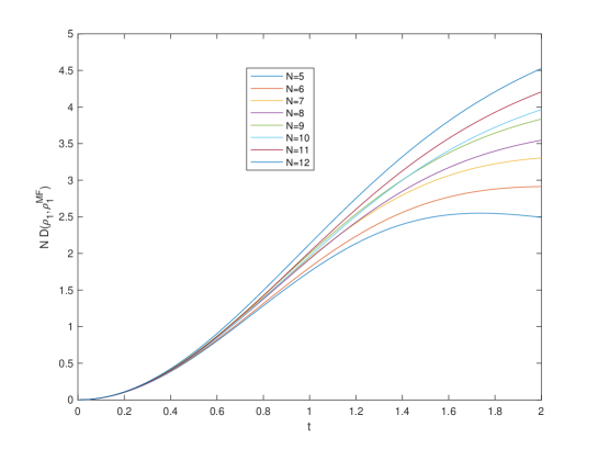
Figure 1: $N\ D\left(\rho_{1}(t),\rho_{1}^{MF}(t)\right)$ for various $N$. For each $N$ , trace distance divergence is averaged over random Page states and over the ensemble of $H$. In the second panel, the early time region is shown and compared to $\frac{1}{2}\left(1-\sqrt{2P-1}\right)$ with dashed lines, where the bound (14) is close to being saturated.

Observables

The Hilbert space is the tensor product of individual spin sites $\mathcal{H}=\otimes_{i=1}^{N}\mathcal{H}_{i}$. Under the assumption the system exhibits quantum chaos for typical states, then such a typical state will scramble in a timescale of order $t_{scr}$ and we can use such a state to describe a black hole. In practice, we will simply choose a random unitary vector in the Hilbert space $\mathcal{H}$ to generate candidate black hole states.

To represent an observer (or test particle) entering the black hole, we enlarge the Hilbert space (for example taking $N\to N+1$ and begin in a product state

$$|\psi(0)\rangle=|\psi_{1}\rangle\otimes|\psi_{0}^{bh}\rangle$$ (7)

where $|\psi_{1}\rangle$ is the spin state representing the observer, and is chosen to be $|\uparrow\rangle$ and $|\psi_{0}^{bh}\rangle$ describes the state of the black hole. The Hamiltonian $H$ generates the exact time evolution of the system. However in a scrambling time the observer’s spin becomes entangled with the black hole. Certainly with respect to the original local basis, the observer’s reduced density matrix becomes highly mixed, and they do not experience the expected laws of quantum mechanics following from time evolution along a bulk geodesic. On the other hand, the efficient averaging of the maximally non-local interaction suggests mean field can be appropriate. As we now see, this leads to evolution that preserves the pure state tensor structure (7), as we would expect for a particle moving along a bulk geodesic.

III Mean Field Versus Exact Evolution

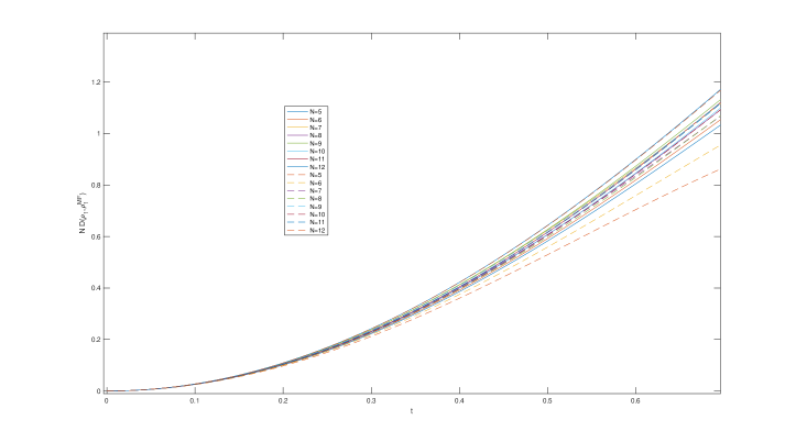
Figure 2: The trace distance (solid lines) is compared to the purity bound $\frac{1}{2}\left(1-\sqrt{2P-1}\right)$ (dashed lines). The bound (14) is close to being saturated.

The mean field Hamiltonian is defined as

$$H^{MF}(t)=\sum_{i=1}^{N}H_{i}^{MF}(t)=\sum_{i=1}^{N}Tr_{i^{c}}(H\rho^{MF}(t)),$$ (8)

where $\rho^{MF}(t)$ is the unitary time evolution of the same initial state evolved by mean field Hamiltonian, and satisfies the von Neumann equation

$$\dfrac{d\rho^{MF}(t)}{dt}=-i\left[H^{MF}(t),\rho^{MF}(t)\right].$$ (9)

Note that each $H_{i}^{MF}$ is a local operator in the Hilbert subspace associated with spin $i$. The trace is over the complement $i^{c}$ to the Hilbert subspace associated with spin $i$. The mean field time evolution is therefore guaranteed to preserve the product form (7). However this operator depends on the state of the other spins, so the time evolution (9) is inherently nonlinear.

The mean field state will deviate from the exact time evolution. To measure this deviation, one can consider the trace distance between reduced density matrices

$$D(\rho_{1}(t),\rho_{1}^{MF}(t))\equiv\frac{1}{2}\left\|\rho_{1}(t),\rho_{1}^{MF}(t)\right\|_{1}=\frac{1}{2}\mathrm{Tr}\,\sqrt{\left(\rho_{1}(t)-\rho_{1}^{MF}(t)\right)^{2}}$$

which offers a metric to measure distinguishability between two quantum states. In the case $\rho_{1}^{MF}(t)$ is a pure state, as is the case here, the trace distance is bounded from below by $\dfrac{1}{2}(1-\sqrt{2P-1})$ where $P$ is the purity of $\rho_{1}(t)$, as shown in appendix A.

Trace distance may also be bounded from above by a Lieb-Robinson bound (Lashkari:2011yi, ; Lowe:2017ehz, ). Combining the purity bound with Lieb-Robinson bound we obtain

$$\dfrac{8}{3N}t^{2}<D\left(\rho_{1}(t),\rho_{1}^{MF}(t)\right)<\dfrac{c^{\prime}}{N}e^{ct}.$$ (10)

Here $c$ and $c^{\prime}$ are constants independent of $N$. This is enough to ensure that the decoherence is an $1/N$ effect. If the exponential behavior is saturated from early times to times well before the purity levels off at $1/2$, the scrambling timescale (4) will emerge, as the timescale over which the trace distance increases to some fixed fraction (say $10\%$ for example). The trace distance between these density matrices measures what is usually termed decoherence of the pure probe state at site 1. However because the interactions are maximally non-local, in this particular model, we expect this to also be a good measure of the global thermalization properties of the system, and hence we will use this method to define our notion of scrambling time. As we will see later, it corresponds well to other definitions considered in the literature.

In figure 1 we plot $N\>D\left(\rho_{1}(t),\rho_{1}^{MF}(t)\right)$ which clearly indicates the universal behavior for early times. Eventually the trace distance saturates, as the purity of $\rho_{1}(t)$ approaches its minimum of $1/2$. The time at which this saturation occurs increases with $N$ as expected from (10).

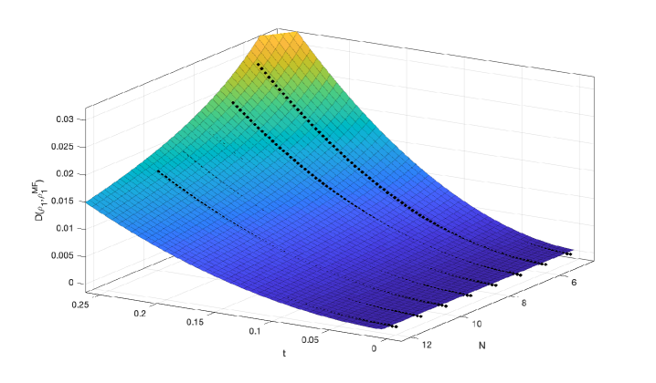
Figure 3: Fit of the averaged trace distance, as a function of time $t$ and $N$. The surface shows a fit to $at^{2}/N$ where $a\approx 2.6$ in good agreement with the $8/3$ prediction.

Following (Yao:2016ayk, ) one my try a fit of $D\left(\rho_{1}(t),\rho_{1}^{MF}(t)\right)$ to the phenomenologically motivated exponential form

$$D\left(\rho_{1}(t),\rho_{1}^{MF}(t)\right)=a\left(e^{bt}-1\right)^{\Delta}N^{-\gamma}$$ (11)

which yields the values $a=5.5,\,b=0.5,\Delta=1.8$ and $\gamma=.92$. The value for $\gamma$ is consistent with the analytic bounds (10). The values for the other parameters are not well determined when looking at the early time limit. Instead a better fit is obtained simply by the quadratic form

$$D\left(\rho_{1}(t),\rho_{1}^{MF}(t)\right)=\frac{a}{N}t^{2}$$

which yields a better least squares fit with fewer parameters, with $a=2.6$, agreeing well with the $8/3$ prediction of appendix (A). With this purely quadratic form we do not see evidence of fast scrambling until we exit this early time limit. In fact, the quadratic approximation holds very well up until just before the point of inflection in the curves. This point of inflection then provides one means of defining the scrambling time. As we see later this matches well with some alternative measures we study below, which indicate the model does indeed fast scramble with in a timescale of order $\log N$. In the meantime, we see the results establish the validity of the mean field approximation in the window of time prior to the scrambling time.

Rather than study the trace distance between mean field and exact evolution for a subsystem (in this case a single qubit) we can instead examine the trace distance between the mean field evolution and the exact evolution of the full global state over the $N$ qubits. In line with the expectations of (Hayden:2007cs, ) we expect a rapid deviation to emerge. We find a linear increase in the trace distance, saturating at late times, with behavior largely independent of $N$.

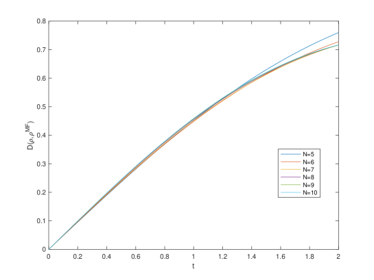
Figure 4: Trace distance between mean field and exact evolution for the global state.

The behavior of the purity of $\rho_{1}(t)$, $P(t)=\mathrm{Tr}\rho_{1}^{2}$ is shown in figure 5. The eigenvalues of the Hamiltonians are sufficiently dense, due to the choice of random couplings, that no recurrence is observed over the time range explored. This is an improvement over (Lowe:2017ehz, ), though the early time results there remain valid despite the simplicity of those models.

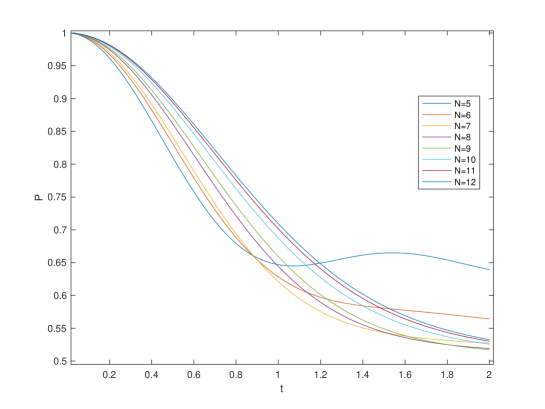
Figure 5: Purity of $\rho_{1}(t)$ for various values of $N$. For $N>6$ these approach $1/2$ monotonically, as expected for a system exhibiting quantum chaos.

Finally we show a fit of the purity as a function of $t$ and $N$, verifying the form valid for early times found in appendix A. Fitting the form

$$P(t)=1-aN^{-\delta}t^{2}$$

for early times yields $\delta=-0.8$ and $a=-2.8$. Errors with the expected form arise from the relatively small values of $N$ considered. Rounding errors also play a role for larger values of $N$.

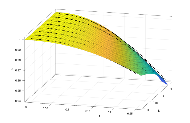
Figure 6: Purity on the probe site as a function of time $t$ and $N$. Fit to $1-at^{2}/N$ with $a\approx 5.3$ close to the prediction of $16/3$ of appendix A.

In summary, we have studied numerically and analytically the trace distance between the mean field and exact evolution for states corresponding to local probes of black holes in this model. We see the trace distance remains small for a timescales shorter than the scrambling time (4). We have also shown the trace distance is bounded below by the purity, which depends only on decoherence of a local spin with respect to the exact time evolution. Moreover this bound is apparently saturated at early times. These results are consistent with the holographic interpretation of the mean field as a bulk worldline Hamiltonian advocated in (Lowe:2017ehz, ). At this level of approximation the mean field approximation is essentially free evolution (more generally an arbitrary local Hamiltonian can be chosen without changing the validity of mean field). In future work, we consider adding nearest neighbor interactions to the spin model to reproduce local field theory interactions in the bulk. For now we turn to a study of the extent to which one sees evidence for fast scrambling in this class of models.

IV Evidence For Fast Scrambling

The observables studied above are arguably simply studying the thermalization of the subsystem as interactions place it in contact with the rest of the system, which acts as the environment, decohering the subsystem. For a general Hamiltonian, those observables would not be indicative of global scrambling or quantum chaos. However for the particular class of Hamiltonians studied here, which are maximally non-local, we find the results match well with other diagnostics of scrambling studied in the literature. We now turn to the study of these observables.

OTOC

The Out-Of-Time-Order-Correlator (OTOC) is one of the first studied diagnostics of quantum chaos (larkin1969quasiclassical, ), where it was noticed that chaotic dynamics can lead to exponential variation in such quantities. In particular, the expectation value of the square of the commutator of a pair of Hermitian operators $V$ and $W$, $C_{2}(t)=\langle[W(t),V(0)]^{\dagger}[W(t),V(0)]\rangle$ is expected to grow exponentially in time: $C_{2}(t)\sim e^{\lambda_{L}t}$. Here $\lambda_{L}$ is to be identified as an analog of a Lyapunov exponent. Here we study this quantity where $V=s_{z,1}$ and $W=s_{z,2}$.

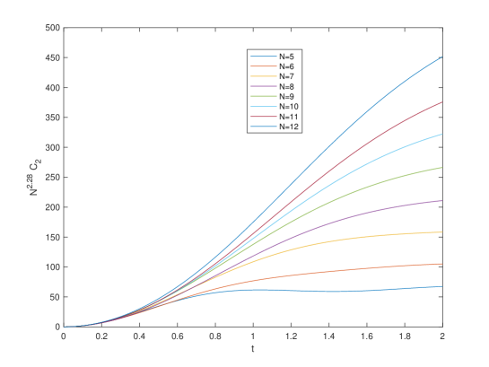
Figure 7: Commutator $C_{2}(t)$ as a function of time for various values of $N$. The result has been rescaled by $N^{2.28}$ to illustrate the universal early time behavior, prior to saturation/scrambling in the late time regime.

For early time evolution, each line can be fitted by $at^{2}/N^{\delta}$, where $a$ and $\delta$ are fitting coefficients.

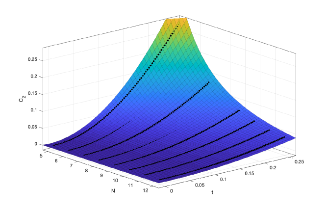
Figure 8: Here the OTOC is fit to the form $at^{2}/N^{\delta}$ with $a\approx 175\pm 4,\,\delta\approx 2.28\pm 0.02$, showing the early time growth of the commutator.

The growth in $C_{2}(t)$ provides the first hint of scrambling. For the numerically accessible values of $N$ the expected exponential growth seems to saturate well before there is a clear separation from the perturbative early time regime (which is only sensitive to the $t^{2}$ term in an expansion around $t=0$). The behavior of $C_{2}$ is qualitatively very similar to the behavior of the trace distance (exact vs. mean field) considered in the previous section. To do better in measuring the scrambling timescale, our strategy will be to perform a measurement of the cross-over timescale between these different regimes, and we will study observables where this cross-over can be measured with greater precision.

Entanglement Entropy

Since the Hamiltonian is maximally non-local in the spin basis, we expect studying the entanglement entropy of pairs of spins provides a useful measure of the global entanglement of the system, and hence the extent to which scrambling has taken place. Recalling that we start the system in a product pure state (7) we can compute the entanglement entropy of the spin at site 1, via

$$S_{ent}(t)=-Tr\left(\rho_{1}\ln\rho_{1}\right).$$

Below we carry out numerical simulations of the system to obtain entropy growth as a function of holographic time as shown in figure 10.

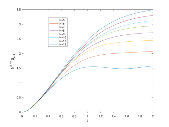
Figure 9: Entanglement entropy as a function of time for various $N$. For each $N$ entropy growth is averaged over random Page states and over the ensemble of $H$. A rescaling by $N^{.67}$ illustrates the universality of the early time regime.Early time regime, fit well by $at^{\gamma}/N^{\delta}$ with $a\approx 3.7\pm 0.1,\gamma\approx 1.62\pm 0.01,\delta\approx 0.67\pm 0.01$

Entanglement entropy growth in a strongly coupled gapless system with a gravity dual has been studied intensely in (Casini:2015zua, ; Liu:2013iza, ; Liu:2013qca, ). It was proposed that the growth in entanglement entropy can be visualized as the spreading of an “entanglement tsunami”. The region covered by the wave-front is entangled with the rest of the system, and the system achieves saturation when fully covered by the tsunami. For a wide class of black hole systems, entropy growth exhibit three stages of development: 1. pre-local-equilibration quadratic growth; 2. post-local equilibration linear growth; 3. saturation, exactly matched by our numeric simulation. It was discussed in (Liu:2013iza, ) that the linear growth regime characterizes the late-time memory loss: the wave front forms a uniform circle and propagates in the same way regardless of what the initial configuration is. For us, we are interested in this timescale to reach the linear regime. From the data in fig. 9 we can study the position where the point of inflection of the curves.

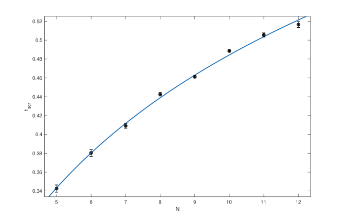
Figure 10: Scrambling time extracted from entropy as a function of $N$.

The results are shown in figure 10. The timescale shows an obvious $\log N$ dependence $t_{scr}=0.21\log N$. We note this one parameter fit produces a better fit than a three parameter power law fit $aN^{\delta}+c$, which offers the strongest numerical evidence of fast scrambling we have found. The entanglement entropy does not depend on a choice of operators (as in the OTOC) nor on the mean field approximation (as in the previous section), so for us is the most numerically useful quantity to study in the approach to global scrambling.

V Summary

We have explored a four-spin interacting system that exhibits fast scrambling feature in the high temperature limit which is conjectured to be holographically dual to a black hole spacetime in the vicinity of the horizon. This is in contrast with SYK model, where chaotic behaviors emerge when the couplings $\beta J$ are taken to be large, corresponding to a low temperature limit, and holographically to a complete asymptotically anti-de Sitter spacetime. We extend early work of the mean field construction to this new holographic Hamiltonian. The trace distance between the exact and mean field Hamiltonian remain small for at least a scrambling time which indicates the local mean field viewpoint, which may be reinterpreted in terms of a bulk description can be valid for timescales smaller than the scrambling time. This supports the conjecture that decoherence of the in-falling state is a dual to the disruptive bulk effects near the space-time singularity.

Appendix A Bounding the Trace Distance

For a density matrix $\rho$, the purity is defined by

$$P(t)=\mathrm{Tr}\rho^{2}\,.$$ (12)

The purity may be computed in an early time expansion following (Kim1996, )

$$P(t)=1-2t^{2}\left(\left\langle H\right\rangle_{\psi}^{2}+\left\langle H^{2}\right\rangle_{\psi}-\left\langle\left\langle H\right\rangle_{\psi_{1}}^{2}\right\rangle_{\psi_{2}}-\left\langle\left\langle H\right\rangle_{\psi_{2}}^{2}\right\rangle_{\psi_{1}}\right)+\mathcal{O}(t^{4})$$

where we have a pure state $\left|\psi\right\rangle=\left|\psi_{1}\right\rangle\times\left|\psi_{2}\right\rangle$ and use the notation for partial matrix elements $\left\langle H\right\rangle_{\psi_{k}}=\left\langle\psi_{k}\left|H\right|\psi_{k}\right\rangle$. If we approximate this formula using an average over Page states, subject to the normalization (3) we obtain

$$P(t)\approx 1-\frac{16t^{2}}{3N}+\mathcal{O}(t^{4})\,.$$

We may use the purity to bound the trace distance

$$D(\rho,\rho^{\prime})=\frac{1}{2}\left\|\rho-\rho^{\prime}\right\|_{1}$$

which is our most refined observable used to define global thermalization. To do this in the examples studied here, we may use the geometric representation of a general mixed state on the single qubit on site 1 as a point $\vec{a}$ on (or inside) the Bloch sphere (MARINESCU2012221, )

$$\rho=\frac{1}{2}\left(\mathbbm{1}+\vec{a}\cdot\vec{\sigma}\right)\,.$$ (13)

In that representation the trace distance becomes half the Euclidean distance between the points. The initial state is a pure state on the unit Bloch sphere, represented by a vector $\vec{a}$ with $\vec{a}^{2}=1$. As scrambling proceeds, $\rho(t)$ becomes a mixed state represented by a vector $\vec{b}$ with $\vec{b}^{2}<1$. This implies

$$D(\rho(t),\rho_{MF}(t))\geq D(\rho_{1}(t),\rho_{MF,1}(t))\geq\frac{1}{2}\left(1-|\vec{b}|\right)$$

using the triangle inequality to bound the minimum distance between the points. The purity of (13) is

$$P(t)=\frac{1}{2}\left(1+\vec{b}^{2}\right)$$

so

$$D(\rho(t),\rho_{MF}(t))\geq\frac{1}{2}\left(1-\sqrt{2P-1}\right)\,.$$ (14)

Approximating this for early times when $P$ is close to 1, gives

$$D(\rho(t),\rho_{MF}(t))\geq\frac{1}{2}\left(1-P\right)\approx\frac{8t^{2}}{3N}\,.$$

References

- (1) O. Aharony, S. S. Gubser, J. M. Maldacena, H. Ooguri, and Y. Oz, “Large N field theories, string theory and gravity,” Phys. Rept. 323 (2000) 183–386, arXiv:hep-th/9905111 [hep-th].
- (2) A. Hamilton, D. N. Kabat, G. Lifschytz, and D. A. Lowe, “Local bulk operators in AdS/CFT: A Boundary view of horizons and locality,” Phys. Rev. D73 (2006) 086003, arXiv:hep-th/0506118 [hep-th].
- (3) A. Hamilton, D. N. Kabat, G. Lifschytz, and D. A. Lowe, “Holographic representation of local bulk operators,” Phys. Rev. D74 (2006) 066009, arXiv:hep-th/0606141 [hep-th].
- (4) D. A. Lowe and L. Thorlacius, “Black hole complementarity: The inside view,” Phys. Lett. B737 (2014) 320–324, arXiv:1402.4545 [hep-th].
- (5) D. A. Lowe and L. Thorlacius, “Quantum information erasure inside black holes,” JHEP 12 (2015) 096, arXiv:1508.06572 [hep-th].
- (6) D. A. Lowe and L. Thorlacius, “A holographic model for black hole complementarity,” JHEP 12 (2016) 024, arXiv:1605.02061 [hep-th].
- (7) D. A. Lowe and L. Thorlacius, “Black hole holography and mean field evolution,” JHEP 01 (2018) 049, arXiv:1710.03302 [hep-th].
- (8) G. Bentsen, Y. Gu, and A. Lucas, “Fast scrambling on sparse graphs,” Proc. Nat. Acad. Sci. 116 no. 14, (2019) 6689–6694, arXiv:1805.08215 [cond-mat.str-el].
- (9) K. S. Thorne, R. H. Price, and D. A. Macdonald, eds., BLACK HOLES: THE MEMBRANE PARADIGM. 1986.
- (10) Y. Sekino and L. Susskind, “Fast Scramblers,” JHEP 10 (2008) 065, arXiv:0808.2096 [hep-th].
- (11) N. Lashkari, D. Stanford, M. Hastings, T. Osborne, and P. Hayden, “Towards the Fast Scrambling Conjecture,” JHEP 04 (2013) 022, arXiv:1111.6580 [hep-th].
- (12) N. Y. Yao, F. Grusdt, B. Swingle, M. D. Lukin, D. M. Stamper-Kurn, J. E. Moore, and E. A. Demler, “Interferometric Approach to Probing Fast Scrambling,” arXiv:1607.01801 [quant-ph].
- (13) P. Hayden and J. Preskill, “Black holes as mirrors: Quantum information in random subsystems,” JHEP 09 (2007) 120, arXiv:0708.4025 [hep-th].
- (14) A. Larkin and Y. N. Ovchinnikov, “Quasiclassical method in the theory of superconductivity,” Sov Phys JETP 28 no. 6, (1969) 1200–1205.
- (15) H. Casini, H. Liu, and M. Mezei, “Spread of entanglement and causality,” JHEP 07 (2016) 077, arXiv:1509.05044 [hep-th].
- (16) H. Liu and S. J. Suh, “Entanglement Tsunami: Universal Scaling in Holographic Thermalization,” Phys. Rev. Lett. 112 (2014) 011601, arXiv:1305.7244 [hep-th].
- (17) H. Liu and S. J. Suh, “Entanglement growth during thermalization in holographic systems,” Phys. Rev. D89 no. 6, (2014) 066012, arXiv:1311.1200 [hep-th].
- (18) J. I. Kim, M. C. Nemes, A. F. R. de Toledo Piza, and H. E. Borges, “Perturbative expansion for coherence loss,” Phys. Rev. Lett. 77 (Jul, 1996) 207–210. https://link.aps.org/doi/10.1103/PhysRevLett.77.207.
- (19) D. C. Marinescu and G. M. Marinescu, “Chapter 3 - classical and quantum information theory,” in Classical and Quantum Information, D. C. Marinescu and G. M. Marinescu, eds., pp. 221 – 344. Academic Press, Boston, 2012. http://www.sciencedirect.com/science/article/pii/B9780123838742000035.