Close-in Exoplanets as Candidates of Strange Quark Matter Objects

Abstract

Since the true ground state of the hadrons may be strange quark matter (SQM), pulsars may actually be strange stars rather than neutron stars. According to this SQM hypothesis, strange planets can also stably exist. The density of normal matter planets can hardly be higher than 30 g cm^-3. As a result, they will be tidally disrupted when its orbital radius is less than $\sim 5.6\times 10^{10}\rm\,cm$, or when the orbital period ($P_{\rm orb}$) is less than $\sim\rm 6100\,s$. On the contrary, a strange planet can safely survive even when it is very close to the host, due to its high density. The feature can help us identify SQM objects. In this study, we have tried to search for SQM objects among close-in exoplanets orbiting around pulsars. Encouragingly, it is found that four pulsar planets (XTE J1807-294 b, XTE J1751-305 b, PSR 0636 b, PSR J1807-2459A b) completely meet the criteria of $P_{\rm orb}<\rm 6100\,s$, and are thus good candidates for SQM planets. The orbital periods of two other planets (PSR J1719+14 b and PSR J2051-0827 b) are only slightly higher than the criteria. They could be regarded as potential candidates. Additionally, we find that the periods of five white dwarf planets (GP Com b, V396 Hya b, J1433 b, WD 0137-349 b, and SDSS J1411+2009 b) are less than 0.1 days. We argue that they might also be SQM planets. It is further found that the persistent gravitational wave emissions from at least three of these close-in planetary systems are detectable to LISA. More encouragingly, the advanced LIGO and Einstein Telescope are able to detect the gravitational wave bursts produced by the merger events of such SQM planetary systems, which will provide a unique test for the SQM hypothesis.

1 Introduction

Soon after the discovery of neutrons, the existence of neutron stars (NS), which are mainly made up of neutrons, was predicted. In 1960’s, pulsars were discovered. As extremely compact objects with a typical mass of $\sim 1.4M_{\odot}$ and a typical radius of only about $10\rm\,km$, they were soon identified as neutron stars. However, it has also been argued that the true ground state of the matter at extreme densities may actually be quarks (Itoh, 1970; Bodmer, 1971) rather than the hadronic form. The internal composition of these extremely compact stars thus is still largely unclear. For instance, under such an extreme condition, some particles like hyperons, baryons, and even bosons may appear; quark deconfinement may also happen. In particular, it has long been suggested that even more exotic states such as strange quark matter (SQM) may exist in the core (Itoh, 1970; Bodmer, 1971; Witten, 1984; Farhi & Jaffe, 1984). Recently, the discovery of several $2M_{\odot}$ pulsars (Demorest et al., 2010; Antoniadis et al., 2013; Cromartie et al., 2019) attracts the attention of scientists. Pulsars with such a high mass and a small radius imply that the density at the center can reach several times of nuclear saturation density, which further complicates the internal composition of these compact stars.

Following the SQM hypothesis, the existence of a whole sequence of SQM objects, such as strange quark stars (SSs) (Witten, 1984; Farhi & Jaffe, 1984; Alcock, 1986), strange quark dwarfs (Glendenning et al., 1995a, b), and strange quark planets (Glendenning et al., 1995a, b; Xu & Wu, 2003; Horvath, 2012; Huang & Yu, 2017) are predicted. For example, Jiang et al. (2018) argued that the double white dwarf binary J125733.63+542850.5 may actually contains two strange dwarfs. SQM objects may be covered by a thin crust of normal hadronic matter, or may even simply be bare SQM cores (Glendenning et al., 1995a, b). The common compact nature of SSs and NSs makes it difficult to discriminate these two kinds of internally different stars observationally (Alcock, 1986). A few efforts have been made to reveal the difference between them. For example, they may have different $M-R$ relations (Witten, 1984; Krivoruchenko, 1991; Glendenning et al., 1995a; Li et al., 1995; de Avellar & Horvath, 2010; Drago et al., 2014), and SSs may rotate much faster (with spin period $P_{\rm spin}<1\rm ms$) than NSs (Friedman et al., 1989; Frieman & Olinto, 1989; Glendenning, 1989; Kristian et al., 1989; Madsen, 1998; Dai & Lu, 1995a, b; Sawyer, 1989; Bhattacharyya et al., 2016). They may also have different cooling rates (Pizzochero, 1991; Page & Applegate, 1992; Ma et al., 2002), different gravitational wave (GW) features (Jaranowski et al., 1998; Madsen, 1998; Lindblom & Mendell, 2000; Andersson et al., 2002; Jones & Andersson, 2002; Bauswein et al., 2010; Moraes & Miranda, 2014; Geng et al., 2015; Mannarelli et al., 2015), different maximum masses (Lai & Xu, 2009; Li et al., 2010; Weissenborn et al., 2011; Mallick, 2013; Zhu et al., 2013; Zhou et al., 2018; Shibata et al., 2019), and so on. Nevertheless, due to the impracticability of the above methods at the current stage, the problem still remains unsolved.

Encouragingly, several new methods were recently proposed to distinguish SSs from NSs. The basic idea involves the tremendous difference between SQM planets and normal matter ones. Because of the extreme compactness, an SQM planet can be very close to its host SS star, without being tidally disrupted. It can even emit strong GW signals when it finally spirals-in and merges with the host star(Geng et al., 2015). GW emission from these merging SQM planets within our Galaxy can be detected by GW detectors such as advanced LIGO and the future Einstein Telescope. It is thus suggested that we could identify SQM objects by searching for very close-in planets around pulsars (Huang & Yu, 2017), or by detecting GW bursts from merging SQM planet systems (Geng et al., 2015).

It is interesting to note that nearly ten GW events from merging double black holes (and even one from merging double neutron stars) have been detected by advance LIGO and Virgo since 2016 (Abbott et al., 2016, 2017). Recently, advanced LIGO has just begun a new observational run, which will surely come up with much more GW events. The great breakthrough in GW astronomy hopefully sheds light on possible detection of GW emission from merging SQM planet systems in the near future. At the same time, rapid progress in observational technology also leads to a drastic increase in the number of extrasolar planets being detected in the past decades. Interestingly, a good number of exoplanets are found to be orbiting around pulsars. In this study, we examine these pulsar planets systematically to search for very close-in ones that could be ideal candidates for SQM objects. The possibility of detecting GW emission from these candidates will also be explored.

The structure of our paper is organized as follows. In Section 2, the background relevant to SQM planet systems is briefly introduced. In Section 3, we describe the data source of our sample. In Section 4, SQM candidates are selected and evaluated by considering the criteria of close-in introduced in Section 2. GW emission from the candidate SQM planet systems is calculated and compared with the limiting sensitivities of current and future GW experiments in Section 5. Finally, Section 6 presents our conclusions and discussion.

2 Theories relevant to SQM planet systems

2.1 Criteria for identifying SQM planets

Table 1: Candidate pulsar planets and their host pulsars.

Planet name	Mass	$P_{\rm orb}$	Host name	Distance	Mass	$Ref.$
	$m$ ($M_{\rm jup}$)	(day)		$d$ ($\rm pc$)	$M$ ($M_{\odot}$)
Gold sample
PSR 0636 b	8	0.067	PSR J0636	210	1.4	1, 2, 3
PSR J1807-2459A b	9.4	0.07	PSR J1807-2459A	2790	1.4	4, 5, 6, 7
PSR 1719-14 b	1	0.090706293	PSR 1719-14	1200	1.4	3, 8, 9
PSR J2322-2650 b	0.7949	0.322963997	PSR J2322-2650	230	1.4	3
PSR 1257+12 b	0.00007	25.262	PSR 1257+12	710	1.4	10, 11, 12, 13, 14
PSR 1257+12 c	0.013	66.5419	PSR 1257+12	710	1.4	10, 11, 12, 13, 14
PSR 1257+12 d	0.012	98.2114	PSR 1257+12	710	1.4	10, 11, 12, 13, 14
PSR B0943+10 b	2.8	730	PSR B0943+10	890	1.5	15
PSR B0943+10 c	2.6	1460	PSR B0943+10	890	1.5	15
PSR B0329+54 b	0.0062	10139.34	PSR B0329+54	1000	1.4	16, 17, 18
PSR B1620-26(AB) b	2.5	36525	PSR B1620-26(AB)	3800	1.35	19, 20, 21, 22, 23
Silver sample
PSR J2051-0827 b	28.3	0.099110266	PSR J2051-0827	1280	1.4	7, 24
PSR J2241-5236 b	12	0.14567224	PSR J2241-5236	500	1.35	7, 25
PSR B1957+20 b	22	0.38	PSR B1957+20	1530	1.4	7, 26
Copper sample
XTE J1807-294 b	14.5	0.0278292	XTE J1807-294	5500	1.5	27, 28, 29, 30, 31, 32
XTE J1751-305 b	27	0.02945997	XTE J1751-305	11000	1.7	33, 34, 35
PSR J1544+4937 b	18	0.12077299	PSR J1544+4937	3500	1.7	36, 37
PSR J1446-4701 b	23	0.277666077	PSR J1446-4701	1500	1.4	38, 39, 40
PSR J1502-6752 b	26	2.48445723	PSR J1502-6752	4200	1.4	38, 39

Note. — $Ref.\,$: (1) Stovall et al. (2014); (2) Spiewak et al. (2016); (3) Spiewak et al. (2018); (4) D’Amico et al. (2001); (5) Ransom et al. (2001); (6) Lynch et al. (2012); (7) Ray & Loeb (2017); (8) Bailes et al. (2011); (9) Martin et al. (2016); (10) Wolszczan & Frail (1992); (11) Wolszczan (1994); (12) Wolszczan (2012); (13) Patruno et al. (2017); (14) Wolszczan (2018); (15) Suleymanova & Rodin (2014); (16) Demianski & Proszynski (1979); (17) Shabanova (1995); (18) Starovoit & Rodin (2017); (19) Thorsett et al. (1993); (20) Lewis et al. (2008); (21) Mottez & Heyvaerts (2011); (22) Schneider et al. (2011); (23) Veras (2016); (24) Stappers et al. (1996); (25) Keith et al. (2011); (26) Reynolds et al. (2007); (27) Markwardt et al. (2003a, b); (28) Campana et al. (2003); (29) Kirsch et al. (2004); (30) Falanga et al. (2005); (31) Riggio et al. (2007); (32) Patruno et al. (2010); (33) Markwardt et al. (2002); (34) Gierliński & Poutanen (2005); (35) Andersson et al. (2014); (36) Bhattacharyya et al. (2013); (37) Tang et al. (2014); (38) Keith et al. (2012); (39) Ng et al. (2014); (40) Arumugasamy et al. (2015).

Table 2: White dwarf planets with $P_{\rm orb}<0.1$ days and their host stars.

Planet name	Mass	$P_{\rm orb}$	Host name	Distance	Mass	$Ref.$
	$m$ ($M_{\rm jup}$)	(day)		$d$ ($\rm pc$)	$M$ ($M_{\odot}$)
GP Com b	26.2	0.032	GP Com	75	0.33	1, 2, 3, 4
V396 Hya b	18.3	0.045	V396 Hya	77	0.32	2, 3, 4, 5
J1433 b	57.1	0.054	J1433	226	0.8	3, 4, 6, 7
WD 0137-349 b	56	0.07943002	WD 0137-349	102.26	0.39	8, 9, 10, 11
SDSS J1411+2009 b	50	0.0854	SDSS J1411+2009	177	0.53	12, 13, 14

Note. — $Ref.\,$: (1) Nather et al. (1981); (2) Kupfer et al. (2016); (3) Wong et al. (2018); (4) Cunha et al. (2018); (5) Ruiz et al. (2001); (6) Littlefair et al. (2006); (7) Santisteban et al. (2016); (8) Maxted et al. (2006); (9) Burleigh et al. (2006); (10) Casewell et al. (2015); (11) Longstaff et al. (2017); (12) Drake et al. (2010); (13) Beuermann et al. (2013); (14) Littlefair et al. (2014).

The tidal disruption radius of a planet by its host star is mainly dependent on the density ($\rho$) of the planet and the mass of the central host star ($M$). It can be expressed as $r_{\rm td}\approx\left(\frac{6M}{\pi\rho}\right)^{1/3}$ (Hills, 1975). If the planet is an SQM one, which typically has an extremely high density of $\sim\rm 4\times 10^{14}\,g\,cm^{-3}$, then the tidal disruption radius can be estimated as

$$r_{\rm td}\approx 2.37\times 10^{6}\left(\frac{M}{1.4M^{\odot}}\right)^{1/3}$$

$$\times\left(\frac{\rho}{4\times 10^{14}\rm\,g\,cm^{-3}}\right)^{-1/3}\rm cm.$$ (1)

Taking the host star mass as $1.4M_{\odot}$, the above equation tells us that an SQM planet with a density of $\rm 4\times 10^{14}\,g\,cm^{-3}$ will be disrupted only when its orbital radius is less than $2.37\times 10^{6}$ cm, i.e. when it almost comes to the surface of the host pulsar.

On the contrary, normal planets typically have a density of 1 — 10 $\rm g\,cm^{-3}$. If we take $\rm 30\,g\,cm^{-3}$ as an upper limit for the density of normal planets, then the limiting disruption radius is $5.6\times 10^{10}$ cm (Huang & Yu, 2017). In this study, we take this value as a criteria to discriminate normal planets and SQM ones. If a planet is observed to have an orbital radius ($a$) smaller than $5.6\times 10^{10}\rm\,cm$, then it is most likely an exotic strange quark object, but not a normal matter planet. According to the Kepler’s law, such a close-in planet should also have a very small orbital period, $P_{\rm orb}\lesssim 6100\rm\,s$ (Huang & Yu, 2017). Therefore, we could identify candidates of SQM planets by using the criteria of $P_{\rm orb}\lesssim 6100\rm\,s$ and/or $a\lesssim 5.6\times 10^{10}$cm.

2.2 GWs from SQM planet systems

According to general relativity, orbital motion of a binary system can lead to GW emission and spiral-in of the system. The GW emission power of a system with known masses and orbital parameters is,

$$L_{\rm GW}=\frac{32G^{4}}{5c^{5}}\frac{M^{2}m^{2}\left(M+m\right)}{a^{5}}f\left(e\right),$$ (2)

where $c$ is the speed of light, $G$ is the gravitational constant, and $m$ is the mass of the planet. The factor $F\left(e\right)=\left(1+\frac{73}{24}e^{2}+\frac{37}{96}e^{4}\right)/\left(1-e^{2}\right)^{7/2}$ is a function of the orbital eccentricity ($e$). Here we take $F\left(e\right)=1$ for circular orbits considered in our modeling.

In a binary system, the orbit will evolve with time due to continuous GW emission. During this process, the GW strain will increase with time. If the distance of the binary system with respect to us is $d$, then the strain amplitude of the GW can be expressed as (Peters & Mathews, 1963; Postnov & Yungelson, 2014; Geng et al., 2015),

$$h=5.1\times 10^{-23}\left(\frac{M_{C}}{1\,M_{\odot}}\right)^{5/3}\left(\frac{P_{\rm orb}}{1{\rm\,hr}}\right)^{-2/3}\left(\frac{d}{10{\rm\,kpc}}\right)^{-1},$$ (3)

where $M_{C}=\left(Mm\right)^{3/5}/\left(M+m\right)^{1/5}$ is the chirp mass. Directly observable quantity of GW is the strain spectral amplitude. For a binary system, it is given as (Finn & Chernoff, 1993; Nissanke et al., 2010; Postnov & Yungelson, 2014; Geng et al., 2015),

$$h_{f}=6.4\times 10^{-21}\left(\frac{M_{C}}{1M_{\odot}}\right)^{5/6}\left(\frac{f}{300Hz}\right)^{-7/6}$$

$$\times\left(\frac{d}{10\rm\,kpc}\right)^{-1}Hz^{-1/2},$$ (4)

where $f$ is the GW frequency that may evolve with time, $f={2}/{P_{\rm orb}}$.

Because of the continuous energy loss through GW emission, the system will coalesce at the final stage of the inspiraling process. The coalescence time scale (Peters & Mathews, 1963; Peters, 1964; Lorimer, 2008) of the system is expressed as

$${t_{\rm co}}=9.88\times 10^{6}{\rm yr}\left(\frac{P_{\rm orb}}{\rm 1\,hr}\right)^{8/3}\left(\frac{\mu}{1\,M_{\odot}}\right)^{-1}\left(\frac{\mathcal{M}}{1\,M_{\odot}}\right)^{-2/3},$$ (5)

where $\mu={Mm}/\left(M+m\right)$ is the reduced mass, $\mathcal{M}=M+m$ is the total mass of the system.

3 Data collection

In this study, we will systematically examine all the available short period exoplanets to search for possible candidate SQM planets. For this purpose, we have searched through various exoplanet data bases. Currently, popular exoplanet data bases that are widely used in the field include: the Extrasolar Planets Encyclopaedia (hereafter, EU), the NASA Exoplanet Archive (ARCHIVE), the Open Exoplanet Catalogue (OPEN), the Exoplanet Data Explorer (ORG), and Extrasolar planet’s catalogue produced by Kyoto University (EXOKyoto). The numbers of planets in these databases are very different from each other. Interestingly, note that a detailed comparison of these databases has been carried out by Bashi et al. (2018). Generally speaking, EU seems to provide the most complete sample for exoplanets. There are totally 6699 planets listed on the EU web site, among which 4011 are confirmed and 2688 are candidates.

Since SQM planets are most likely to be found orbiting around pulsars (in this case, the pulsars themselves should also be strange stars, but not normal neutron stars), we will mainly concentrate on pulsar planets. So, as the initial step, we first select all the candidates of pulsar planets. In this aspect, the EU data base contributes most of the objects. There are 18 pulsar planets listed in EU, 6 listed in ARCHIVE, and 3 listed in ORG. The total number of pulsar planet candidates is 19 after considering the overlapping in different databases. In Table 1, we have listed some key parameters of these 19 candidates as well as their host pulsars. Among these objects, 6 planets interestingly have an orbital period less than 0.1 day (i.e., 8640 seconds). Note that our exact period criteria for SQM objects is 6100 s, but we believe that all the planets with $P_{\rm orb}<0.1$ days deserve being paid special attention to.

The nature of companions around pulsars is actually not easy to be well defined. A companion of several Jupiter mass could be a massive planet, but it could also be a small white dwarfs. The key problem is that its radius usually could not be accurately measured. As a result, we should bear in mind that the 19 objects listed in Table 1 are only candidates, not confirmed pulsar planets. According to the confidence level, we have divided these 19 objects into three classes, the gold sample, the silver sample, and the copper sample. In the gold sample, there are strong clues supporting the objects as planets. In the silver sample, there are some clues hinting the objects as planets (Ray & Loeb, 2017). In the copper sample, the objects might be planets, but the evidence supporting the idea is highly lacking. Interestingly, we find that three objects in the gold sample and one object in the silver sample have periods less than 0.1 days. We will describe the details of these objects in the next section.

SQM planets may also exist around white dwarfs, because these so called white dwarfs might actually be strange quark dwarfs. So, we also select all the WD planets that have an orbital period less than 0.1 day from EU. The total number of WD planets met such a requirement is 5, as listed in Table 2.

To get an overall picture on how these short period planets differ from others, we have plot all the planets with available masses and orbital periods on the $m$ – $P_{\rm orb}$ plane in Figure 1. It clearly shows that all the planets with a period smaller than 0.1 day are orbiting around pulsars or white dwarfs. This kind of ultra-short period objects form a distinct group and take a special place in the lower right region of Figure 1. It strongly hints that they may have an exotic nature as compared with other planets.

4 Candidates of SQM planets

As explained in Section 2.1, because of the extreme compactness, an SQM object could be very close to its host strange star, without being tidally disrupted. So, closeness is a unique feature of SQM planets. To search for SQM objects, we have selected all the close-in exoplanets around pulsars and WDs. These ultra-short period (period less than 0.1 day) objects are listed in Table 3. To resist tidal disruption, they should have a relatively high mean density. To see how exotic these objects are, we have calculated the minimum mean densities of these objects by using the period-density relation of $\rho_{\rm min}\approx{3\pi}/\left({0.462^{3}GP_{\rm orb}^{2}}\right)$ (Frank et al., 1985; Bailes et al., 2011). The results are also presented in Table 3. We can see that the minimum densities of these objects are all significantly larger than that of normal rocky or iron material (typically with a density of $\rm 1-10\,g\,cm^{-3}$). If these objects are planets but not small white dwarfs, then the possibility that they are SQM objects is very high. Below, we will examine these close-in objects one by one in detail and try to clarify their true nature.

Table 3: Orbital parameters and minimum mean densities of ultra-short period objects

Planet name	$P_{\rm orb}$	Orb. radius	$\rho_{\rm min}$
	(s)	$a$ ($10^{10}\rm\,cm$)	($\rm g\,cm^{-3}$)
XTE J1807-294 b	2404	3.1	247.9
XTE J1751-305 b	2545	3.4	221.2
PSR 0636 b	5789	5.4	42.8
PSR J1807-2459A b	6048	5.6	39.2
PSR 1719-14 b	7837	6.6	23.3
PSR J2051-0827 b	8563	7.1	19.5
GP Com b	2765	2.1	187.5
V396 Hya b	3888	2.6	94.8
J1433 b	4666	4.0	65.8
WD 0137-349 b	6863	4.1	30.4
SDSS J1411+2009 b	7379	4.7	26.3

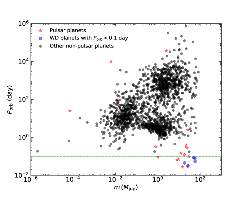
Figure 1: Orbital periods versus masses for all the 1638 exoplanets with data available from the EU web site (http://www.exoplanet.eu/catalog/). The red stars represent candidate pulsar planets. The blue points correspond to the five close-in WD planets with $P_{\rm orb}<0.1$ days, and the black dots represent other 1616 exoplanets.

4.1 Close-in objects around pulsars

The mass of planets can distribute in a very wide range. Some planets can be very massive. In fact, the upper mass limit of planets has been derived by many authors, which could be $43^{+14}_{-23}M_{\rm jup}$ (Grether & Lineweaver, 2006), $42.5M_{\rm jup}$ (Ma & Ge, 2014) and/or $60M_{\rm jup}$ (Hatzes & Rauer, 2015). On the other hand, white dwarf cannot be too small and they should have a lower mass limit. Recently, two low-mass white dwarf were reported, i.e. SDSS J184037.78+642312.3 ($0.17M_{\odot}$) (Hermes et al., 2012a) and SDSS J222859.93+362359.6 ($0.16M_{\odot}$) (Hermes et al., 2012b). They hint that white dwarfs maybe are unlikely to be less than 100 $M_{\rm jup}$. In our Table 1, all the objects are significantly less massive than the planetary mass limits, thus are reasonable candidates for planets.

Among all the close-in candidates in Table 3, three are gold sample objects, one is a silver sample object, and two are copper sample objects. The other five are WD planet candidates. Here, we describe these objects one by one.

4.1.1 Gold sample objects

PSR J0636 b is a companion of the millisecond pulsar PSR J0636+5129 (spin period 2.87 ms) (Stovall et al., 2014). It has a mass of $8M_{\rm\,jup}$. Its orbital period is $\sim 5789\rm\,s$, and the orbital radius is correspondingly $\sim 5.4\times 10^{10}\rm\,cm$. PSR J0636+5129 does not exhibit any eclipses caused by excess material in the system (Stovall et al., 2014; Spiewak et al., 2016; Kaplan et al., 2018). PSR J0636 b is clearly identified as a planet by many authors (Stovall et al., 2014; Spiewak et al., 2016, 2018). It is also explicitly listed as a planet by several planet databases, such as by EU, EXOKyoto, PHLUPR (short for: Planetary Habitability Laboratory of the University of Puerto Rico at Arecibo), GCEXO (short for: a General Catalogue of EXOplanets).

PSR J1807-2459A b is a companion of the millisecond pulsar PSR J1807-2459A (spin period 3.06 ms) (D’Amico et al., 2001; Ransom et al., 2001; Lynch et al., 2012). This object has a mass of $9.4M_{\rm\,jup}$, with an orbital period of $\sim 6048\rm\,s$, and correspondingly an orbital radius of $\sim 5.6\times 10^{10}\rm\,cm$. PSR J1807-2459A shows no eclipses, but one can not rule out the possibility of eclipses at longer wavelengths (Ransom et al., 2001; Lynch et al., 2012). PSR J1807-2459A b is identified as a planet by several authors(D’Amico et al., 2001; Ray & Loeb, 2017). Websites including this object in their planet catalogues are EU, EXOKyoto, PHLUPR, and GCEXO.

PSR 1719-14 b is a companion of the millisecond pulsar PSR J1719-1438 (spin period 5.7 ms) (Bailes et al., 2011; Martin et al., 2016). It has a mass of $1M_{\rm\,jup}$, with an orbital period of $\sim 7837\rm\,s$, and an orbital radius of $\sim 6.6\times 10^{10}\rm\,cm$. It is identified as a planet by many researchers (Bailes et al., 2011; Martin et al., 2016; Spiewak et al., 2018). Websites listing this object in their planet catalogues are EU, ARCHIVE, EXOKyoto, PHLUPR, and GCEXO. PSR J1719-14 b was once considered to be a C/O dwarf in an ultra-compact low-mass X-ray binary (UCLMXB) by Bailes et al. (2011). However, since its mass is very low ($1M_{\rm\,jup}$), it is more likely to be a planetary object. Horvath (2012) explicitly argued that PSR J1719-14 b should be an exotic strange object rather than a C/O dwarf. Very recently, Huang & Yu (2017) also identified PSR J1719-14 b as an ideal candidate of SQM planet.

4.1.2 Silver sample objects

PSR J2051-0827 b is a companion of the millisecond pulsar PSR J2051-0827 (spin period 4.5 ms) (Stappers et al., 1996; Ray & Loeb, 2017). It has a mass of $28.3M_{\rm\,jup}$, with an orbital period of $\sim 8563\rm\,s$, and an orbital radius of $\sim 7.1\times 10^{10}\rm\,cm$. Its mass is within the planetary mass range. While Ray & Loeb (2017) suggested this object as a planet, it has also been argued that it might be a brown dwarf (Stappers et al., 1996). Websites including this object as a planet in catalogues are EU, ARCHIVE, EXOKyoto, PHLUPR, and GCEXO. The orbital period and orbital radius of this object are slightly larger than our strange planet criteria, but we suggest that it might be a good candidate for SQM object and deserves paying special attention to.

4.1.3 Copper sample objects

XTE J1807-294 b is a companion of the millisecond X-ray pulsar XTE J1807-294 (spin period 5.25 ms) (Markwardt et al., 2003a, b; Campana et al., 2003; Kirsch et al., 2004; Falanga et al., 2005; Riggio et al., 2007; Patruno et al., 2010). It has a mass of $14.5\pm 8.5M_{\rm\,jup}$, with an orbital period of $\sim 2404\rm\,s$, and an orbital radius of $\sim 3.1\times 10^{10}\rm\,cm$. No X-ray eclipse was observed from this system (Falanga et al., 2005). According to the mass-radius relation, the companion may be the core of a previously crystallized C/O dwarf (Deloye & Bildsten, 2003). However, there are no emission or absorption lines found from this companion (Campana et al., 2003). This object is listed as a planet in EU and EXOKyoto, but its true nature is still highly unclear.

XTE J1751-305 b is a companion of the millisecond X-ray pulsar XTE J1751-305 (spin period 2.3 ms) (Markwardt et al., 2002; Gierliński & Poutanen, 2005; Andersson et al., 2014). It has a mass of $27\pm 10M_{\rm\,jup}$, with an orbital period of $\sim 2545\rm\,s$, and an orbital radius of $\sim 3.4\times 10^{10}\rm\,cm$. The pulsar show no X-ray eclipses during observations (Markwardt et al., 2002; Gierliński & Poutanen, 2005). This object is listed as a planet in EU and EXOKyoto, but several authors have also argued that it may be the core of a previously crystallized C/O dwarf (Deloye & Bildsten, 2003).

The orbital parameters of both XTE J1807-294 b and XTE J1751-305 b well satisfy our SQM criteria. Also, it is obvious that the masses of both objects are within the planet mass range. Although their true nature is still uncertain, we interestingly notice that Horvath (2012) have argued that an exotic strange object interpretation is the best alternative to a C/O dwarf interpretation for these two objects. We believe that the likelihood of these two objects being SQM planets is high. They need to be studied in more detail in the future.

4.2 Close-in objects around white dwarfs

GP Com b is a companion of the white dwarf GP Com (Nather et al., 1981; Kupfer et al., 2016). Its mass is $26.2\pm 16.6M_{\rm\,jup}$, with an orbital period of $\sim 2765\rm\,s$, and an orbital radius of $\sim 2.1\times 10^{10}\rm\,cm$ (Kupfer et al., 2016). There are suggestions that this object may be a degenerated He dwarf (Nather et al., 1981). But the observed abundances of Ne line from this object could be affected by crystallization processes in the core, and this excludes the highly evolved He donor nature for it (Kupfer et al., 2016). Alternatively, it was argued to be a planet by many authors (Cunha et al., 2018; Wong et al., 2018). Websites listing this object as a planet are EU, EXOKyoto, PHLUPR, and GCEXO.

V396 Hya b is a companion of the white dwarf V396 Hya (Ruiz et al., 2001; Kupfer et al., 2016). The orbital period of the planet is $\sim 3888\rm\,s$, and the orbital radius is $\sim 2.6\times 10^{10}\rm\,cm$. Its mass is measured as $18.3\pm 12.2M_{\rm\,jup}$ (Kupfer et al., 2016). It was suggested to be a degenerated He dwarf (Ruiz et al., 2001), or a crystallized Ne core (Kupfer et al., 2016). However, other authors (Cunha et al., 2018; Wong et al., 2018) have argued that it could be a planet. Websites listing this object as a planet are EU, EXOKyoto, and PHLUPR.

J1433 b is a companion of the white dwarf SDSS J143317.78+101123.3 (WD J1433) (Littlefair et al., 2006; Santisteban et al., 2016). It has an orbital period of $\sim 4666\rm\,s$, and an orbital radius of $\sim 4.0\times 10^{10}\rm\,cm$. Its mass is $57\pm 0.7M_{\rm\,jup}$. It was argued to be a planet by several research groups (Cunha et al., 2018; Wong et al., 2018). Websites listing this object as a planet are EU, EXOKyoto, and PHLUPR. However, note that a few other authors suggested that this object may be an irradiated brown dwarf (Santisteban et al., 2016).

WD 0137-349 b is a companion of the white dwarf 0137-349 (Maxted et al., 2006; Burleigh et al., 2006; Littlefair et al., 2014; Casewell et al., 2015; Longstaff et al., 2017). It has a mass of $56\pm 6M_{\rm\,jup}$, with an orbital period of $\sim 6863\rm\,s$, and an orbital radius of $\sim 4.1\times 10^{10}\rm\,cm$. This object is listed as a planet in EU and EXOKyoto databases. But again note that it was suggested to be an irradiated brown dwarf by several authors (Maxted et al., 2006; Burleigh et al., 2006).

SDSS J1411+2009 b is a companion of the white dwarf SDSS J141126.20+200911.1 (WD J1411). It has a mass of $50\pm 2.0M_{\rm\,jup}$, with an orbital period of $\sim 7379\rm\,s$ and an orbital radius of $\sim 4.7\times 10^{10}\rm\,cm$ (Drake et al., 2010; Beuermann et al., 2013; Littlefair et al., 2014). It is listed as a planet in EU and EXOKyoto databases, but several authors have also suggested it as an irradiated brown dwarf (Beuermann et al., 2013).

Orbital parameters of the above five close-in objects around white dwarfs satisfy the criteria of $P_{\rm orb}<0.1$ day. Their masses are also within the planetary mass range. However, the planetary nature of these objects is still debatable. Especially, they may actually be brown dwarfs. Here, we give some more discussion on this point. In fact, there is no clear boundary between the masses of planets and brown dwarfs. It is well known that the mass of brown dwarfs can range from the Deuterium-burning limit ($0.013M_{\odot}(\sim 13M_{\rm jup})$) to the Hydrogen-burning limit ($0.072M_{\odot}(\sim 75M_{\rm jup})$). The property of a close-in companion is usually seriously affected by the irradiation from its host since it is generally tidally locked (Demory & Seager, 2011; Laughlin et al., 2011; Burgasser et al., 2019). This effect is quite similar for both brown dwarfs and giant planets, thus could not be easily used to discriminate them (Faherty et al., 2013). However, we notice that three of the five objects have extremely small orbital periods. They are GP Com b, V396 Hya b, and J1433 b, and their orbital periods are 2765 s, 3888 s, and 4666 s. As a result, their minimal possible mean density is 187.5 $\rm g/cm^{3}$, 94.8 $\rm g/cm^{3}$, and 65.8 $\rm g/cm^{3}$, respectively. The density is so high that they can hardly be normal brown dwarfs. We argue that at least these three objects are very good candidates for SQM planets.

5 GW from SQM planetary systems

According to general relativity, a binary system continuously emits GW signals due to the orbital motion of the companion. It will lead to an evolution of the orbit, and make the GW emission power increase gradually. At some stage of this gradual process, GW detectors such as LISA (Laser Interferometer Space Antenna) will be able to detect the GW signals from these systems (Cunha et al., 2018; Wong et al., 2018).

For close-in companions orbiting around their hosts, GW emission may be a powerful tool to probe their nature. In this section, we first calculate the persistent GW emissions from the candidate SQM systems in our sample and evaluate the possibility of being detected by the LISA observatory. Then, we also calculate the strength of the catastrophic GW bursts when the candidate SQM systems finally merge due to continuous GW emissions, and compare the results with relevant GW detectors.

5.1 Persistent GWs from SQM planet systems

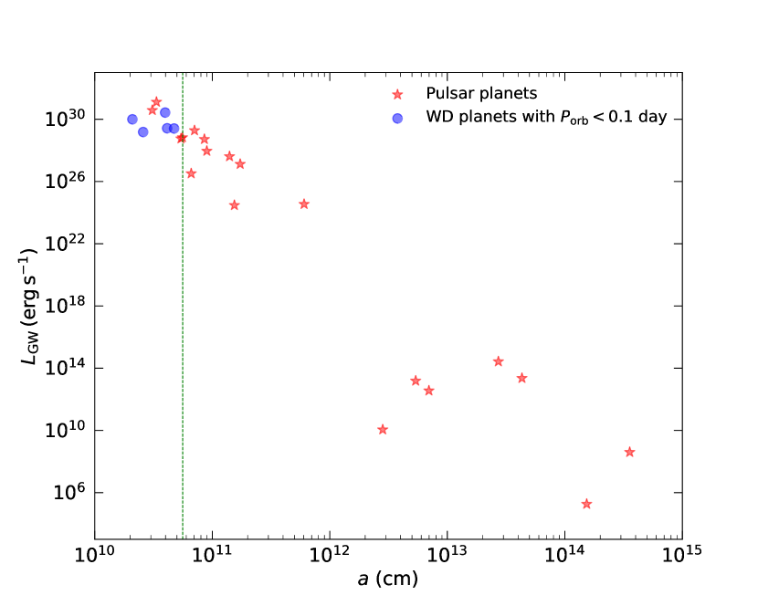
Figure 2: Power of gravitational wave emission versus orbital radius for the planetary systems of our sample. The red stars are pulsar planets and the blue points are WD planets with $P_{\rm orb}<0.1$ day. The vertical green dashed line markes the critical tidal disruption radius of $a=5.6\times 10^{10}\rm\,cm$ for normal matter planets.

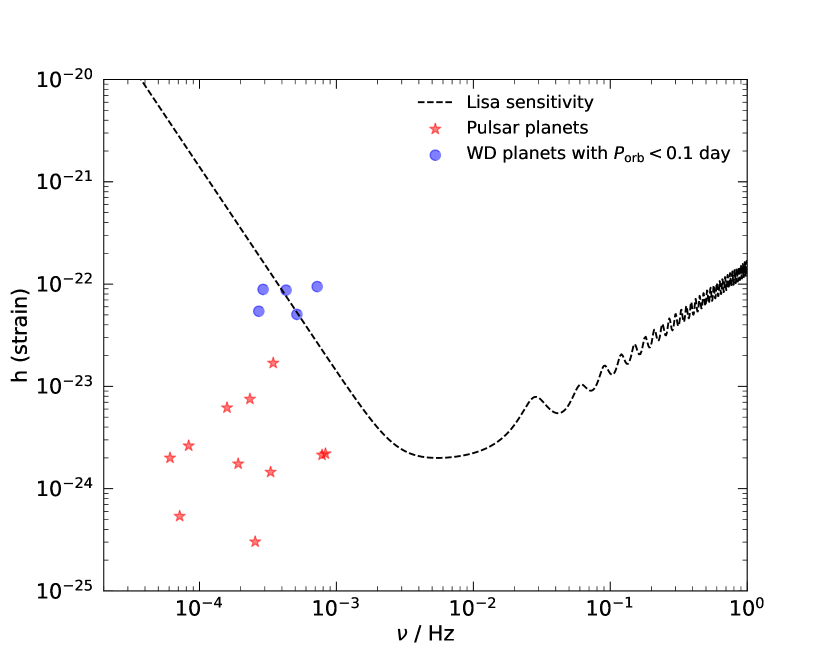
Figure 3: GW strain amplitude versus frequency for the planetary systems of our sample. The blue points represent WD planets with $P_{\rm orb}<0.1$ day and the red stars represent pulsar planets. The black dashed line represents the sensitivity curve of LISA with an one year integration time. For a similar plot, please also see Cunha et al. (2018) and Wong et al. (2018).

For all the planetary systems of our sample, we have calculated their persistent GW luminosity and GW strain amplitude. The results are presented in Table 4. In Figure 2, we plot the GW luminosity versus the orbital radius for them. The red stars and blue points represent pulsar planets and WD planets, respectively. Generally speaking, the orbital radius is a key parameter determining the GW power. For those systems with the orbital radius being less than the critical tidal disruption radius of $5.6\times 10^{10}\rm\,cm$, the GW power is much stronger. Thus there is a hope that GW emission from these systems could be detected by our GW detectors.

In Figure 3, we plot the GW strain amplitude against GW frequency for the planetary systems of our sample. In this plot, the red stars represent pulsar planets and the blue points represent WD planets. The black line is the one-year integration sensitivity curve of LISA . Figure 3 shows clearly that three ultra-short period systems (GP Com b, V396 Hya b and J1433 b) are lying above the sensitivity curve of LISA, thus may hopefully be detected by this powerful GW observatory. The two very close-in systems containing XTE J1807-294 b and XTE J1751-305 b are below the sensitivity curve, since their distances are still too large. If these two systems were located within a distance of $400\rm\,pc$, then they would be detectable to LISA. For close-in planetary systems, GW observation can provide key information on the planet mass, the orbital period, and the orbital radius. We argue that GW observation would be a unique tool to search for SQM candidates. In the future, if a very close-in planet-like object (with the mass being in the planet range, and the orbital period significantly less than 6100 s) could be found orbiting around a stellar object through GW observations, then it must be an SQM planetary system.

Table 4: GW Luminosity, strain amplitude, and coalescence time scale for the planetary systems of our sample.

Planet name	$L_{\rm GW}$	$\rm h$	$t_{\rm co}$
	($\rm egr\,s^{-1}$)		(yr)
XTE J1807-294 b	$3.8\times 10^{30}$	$2.2\times 10^{-24}$	$1.9\times 10^{8}$
XTE J1751-305 b	$1.3\times 10^{31}$	$2.1\times 10^{-24}$	$1.1\times 10^{8}$
PSR 0636 b	$5.7\times 10^{28}$	$1.7\times 10^{-23}$	$3.7\times 10^{9}$
PSR J1807-2459A b	$6.7\times 10^{28}$	$1.5\times 10^{-24}$	$3.5\times 10^{9}$
PSR 1719-14 b	$3.2\times 10^{26}$	$3.0\times 10^{-25}$	$6.6\times 10^{10}$
PSR J2051-0827 b	$1.9\times 10^{29}$	$7.5\times 10^{-24}$	$3.0\times 10^{9}$
PSR J1544+4937 b	$5.2\times 10^{28}$	$1.7\times 10^{-24}$	$6.9\times 10^{9}$
PSR J2241-5236 b	$9.1\times 10^{27}$	$6.2\times 10^{-24}$	$2.0\times 10^{10}$
PSR J1446-4701 b	$4.1\times 10^{27}$	$2.6\times 10^{-24}$	$5.7\times 10^{10}$
PSR J2322-2650 b	$3.0\times 10^{24}$	$5.4\times 10^{-25}$	$2.4\times 10^{12}$
PSR B1957+20 b	$1.3\times 10^{27}$	$2.0\times 10^{-24}$	$1.4\times 10^{11}$
PSR J1502-6752 b	$3.5\times 10^{24}$	$2.5\times 10^{-25}$	$1.7\times 10^{13}$
PSR 1257 12 b	$1.1\times 10^{10}$	$8.4\times 10^{-31}$	$3.1\times 10^{21}$
PSR 1257 12 c	$1.5\times 10^{13}$	$8.2\times 10^{-29}$	$2.2\times 10^{20}$
PSR 1257 12 d	$3.6\times 10^{12}$	$5.8\times 10^{-29}$	$6.7\times 10^{20}$
PSR B0943+10 b	$2.7\times 10^{14}$	$3.0\times 10^{-27}$	$5.8\times 10^{20}$
PSR B0943+10 c	$2.3\times 10^{13}$	$1.7\times 10^{-27}$	$4.0\times 10^{21}$
PSR B0329+54 b	$1.8\times 10^{5}$	$9.7\times 10^{-31}$	$3.1\times 10^{26}$
PSR B1620-26(AB) b	$4.0\times 10^{8}$	$4.3\times 10^{-29}$	$2.4\times 10^{25}$
GP Com b	$9.9\times 10^{29}$	$9.5\times 10^{-23}$	$4.2\times 10^{8}$
V396 Hya b	$1.5\times 10^{29}$	$5.1\times 10^{-23}$	$1.5\times 10^{9}$
J1433 b	$2.7\times 10^{30}$	$8.7\times 10^{-23}$	$4.3\times 10^{8}$
WD 0137-349 b	$2.6\times 10^{29}$	$8.9\times 10^{-23}$	$2.0\times 10^{9}$
SDSS J1411+2009 b	$2.6\times 10^{29}$	$5.4\times 10^{-23}$	$2.2\times 10^{9}$

5.2 GW bursts from merging SQM planet systems

Due to the self-gravity and strong self-bound force of strange quark matter, an SQM planet can get very close to its host without being tidally disrupted by tidal force. During the spiral-in process, the separation between the two objects decreases with time until they merge with each other. At the final merging stage, the system will give birth to a strong GW burst (Geng et al., 2015). In Figure 4, we have plot the strain spectral amplitudes of the GW bursts that will be produced by several candidate SQM planetary systems. Note that these systems are at different distances, and the planets have different masses. For each system, we have used the actually observed parameters in the calculation. We see that the GW amplitudes are all well above the sensitivity curves of both the advanced LIGO and the Einstein Telescope, thus can potentially be detected by these instruments.

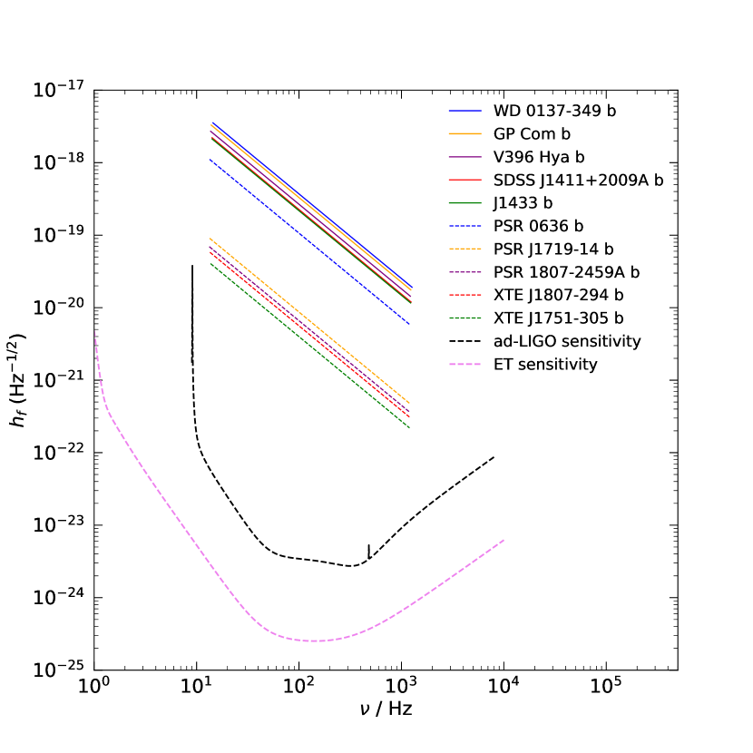
Figure 4: Strain spectral amplitude of the GW bursts for coalescing SS and SQM planet systems. The sensitivity curves of the advanced LIGO and Einstein Telescope are also plotted.

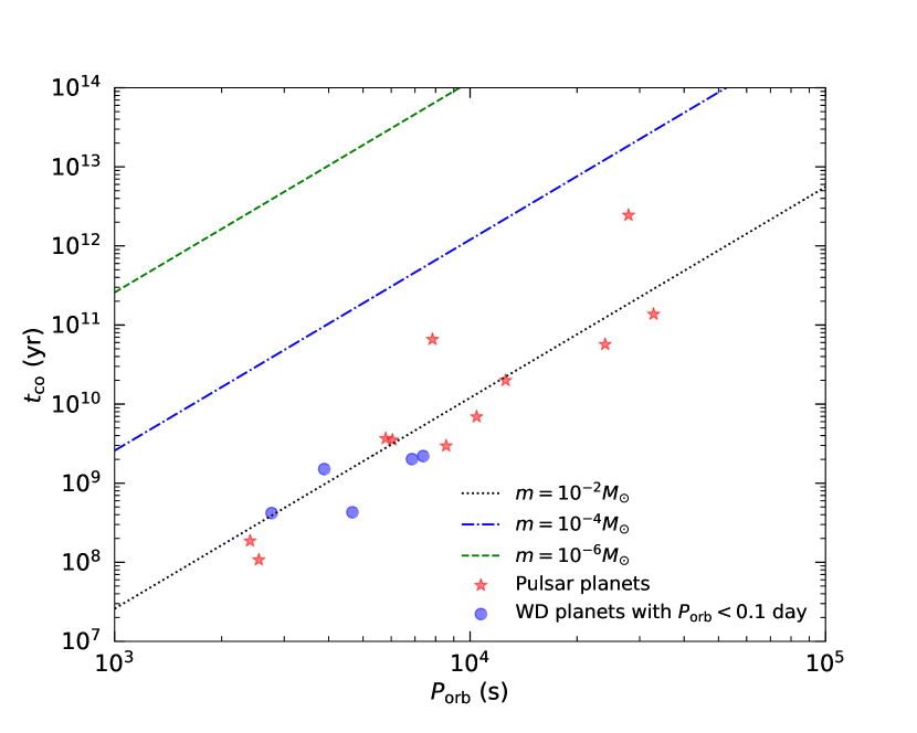
Figure 5: Coalescence timescale versus the initial orbital period for the candidate SQM planetary systems in our sample. Red stars correspond to pulsar planets and blue points correspond to white dwarf planets. The three straight lines illustrate the coalescence timescale for three different planet masses, with the host mass being set as $1.4M_{\odot}$.

The energy loss rate due to GW emission is generally small as compared with the total kinetic energy of the planet. It may take a long time for a planetary system to finally merge. The merger timescale is mainly determined by the orbital radius and the planet mass. In Table 4, we have also calculated the coalescence timescales of the planetary systems in our sample. The results are illustrated in Figure 5. While most systems essentially will not be able to merge even in the lifetime of the Universe, there are about 10 close-in systems that would interestingly merge on a timescale of $10^{8}$ — $10^{9}$ yr. For example, the merger timescale is $\sim 10^{8}$yr for the planetary systems of XTE J1807-294, XTE J1751-305, GP Com b, and J1433 b. Additionally, other factors may be involved and may lead to a much rapid merging process. For example, a pulsar may have multiple planets and the complicate interaction between these companions may speedup the merging processes of some objects (Huang & Geng, 2014).

In short, merging of an SQM planet with its host pulsar can essentially happen on an expectable timescale in our Galaxy. GW emission from these events can be well detected by our current and future detectors. We suggest that searching for GW signals from merging planetary systems could be set as an important goal for advanced LIGO and Einstein Telescope. It deserves extensive efforts since it can provide a unique test for the SQM hypothesis.

6 Conclusions

In this study, we have tried to search for SQM planet candidates among extra-solar planetary systems. The criteria for SQM planets is set as $a<5.6\times 10^{10}\rm\,cm$ and/or $P_{\rm orb}<\rm 6100\,s$. A planet lying closer than this limit with respect to its host will need to have a density significantly larger than 30 g cm^-3 to resist the tidal force, thus is unlikely a normal matter planet, but should be an SQM object. As a result, we find that 11 objects are good candidates for SQM planets, including 3 gold sample objects, 1 silver sample object, 2 cooper sample objects, and 5 white dwarf companions. The three gold sample objects are PSR 0636 b, PSR J1807-2459A b, and PSR J1719-14 b. Their masses are all less than 10 $M_{jup}$ and their possibility of being a planetary object is very high. Among them, although PSR 1719-14 b has a period (7837 s) slightly larger than 6100 s, we still list it as a good candidate since it is essentially in a very close-in orbit. The silver sample object (PSR J2051-0827 b), the two cooper sample objects (XTE J1807-294 b, XTE J1751-305b), and the five white dwarf companions (GP Com b, V396 Hya b, J1433 b, WD 0137-349 b, SDSS J1411+2009 b) are all interesting candidates, but whether they are planetary objects or white dwarfs is still highly uncertain and need further clarification. We have also calculated the GW emissions from these systems. It is found that persistent GW emissions from at least three of them are detectable to LIGO even on a one-year integration. More encouragingly, GW bursts produced at the final merging stage by these candidate SQM planets are well above the sensitivity curves of advanced LIGO and Einstein Telescope. GW observations thus could be a promising strategy for testing the SQM hypothesis.

It is striking to note that our SQM candidates are mainly found around millisecond pulsars. It leads to the interesting conjecture that there might be some intrinsic connection between SQM objects and low mass X-ray binaries (LMXBs). Indeed, some authors (Li et al., 1995; Xu, 2002; Xu & Qiao, 1998; Poutanen & Gierli´nski, 2003; Zhu et al., 2013) have tried to identify SSs in LMXBs. For example, the famous LMXBs of Her X-1 (Li et al., 1995) and SAX J1808.4-3658 have been argued as SS candidates (Li et al., 1999; Poutanen & Gierli´nski, 2003; Gangopadhyay et al., 2012). Poutanen & Gierli´nski (2003) and Gangopadhyay et al. (2012) also noticed the similarity of XTE J1807-294 and XTE J1751-305 with respect to SAX J1808.4-3658 when they argued that SAX J1808.4-3658 should be a strange star. Furthermore, Gangopadhyay et al. (2013) listed 12 stars in binary systems as SSs, again including Her X-1 and SAX 1808.4-3658. Recently, Chen (2016) pointed out that the binary systems of SAX 1808.4-3658 and PSR J1719-1438 may have similar evolutionary history. In fact, the link between strange stars and LXMBs is not difficult to understand theoretically. Continuous accretion and significant mass transfer widely exists in LXMBs. Increase of the mass can easily lead to an ultra-high density at the center of the pulsar, leading to a phase transition and turn the pulsar into a strange quark star even it is originally born as a neutron star.

Pulsars in these close-in binary systems generally show no eclipsing in high-frequency range. There are two possible reasons for this. First, the inclination angle of the orbit should be relatively large. Second, the density of the companion may be high and its radius is correspondingly very small. This will further support the SQM nature of the object. In several cases, possible eclipse is reported to be observed at low-frequency range. The small amount of eclipsing plasma in these cases may come from the ablation of the outer crust of the SQM planet.

7 Acknowledgments

This work was supported by the National Natural Science Foundation of China (Grant Nos. 11873030, 11475085, 11535005, 11690030, and 11703041), by Nation Major State Basic Research and Development of China (2016YFE0129300), and by the Strategic Priority Research Program of the Chinese Academy of Sciences (“multi-waveband Gravitational Wave Universe”, Grant No. XDB23040000).

References

- Abbott et al. (2016) Abbott, B. P., Abbott, R., Abbott, T. D., & Abernathy, M. R. 2016, Phys. Rev. Lett., 116, 061102
- Abbott et al. (2017) Abbott, B. P., Abbott, R., Abbott, T. D., Acernese, F., & Abernathy, M. R. 2017, Phys. Rev. Lett., 119, 161101
- Alcock (1986) Alcock, C. 1986, ApJ, 310, 261
- Andersson et al. (2014) Andersson, N., Jones, D. I., & Ho, W. C. G. 2014, MNRAS, 442, 1786
- Andersson et al. (2002) Andersson, N., Jones, D. I., & Kokkotas, K. D. 2002, MNRAS, 337, 1224
- Antoniadis et al. (2013) Antoniadis, J., Freire, P. C. C., Wex, N., et al. 2013, Science, 340, 448
- Arumugasamy et al. (2015) Arumugasamy, P., Pavlov, G. G., & Garmire, G. P. 2015, ApJ, 814, 90
- Bailes et al. (2011) Bailes, M., Bates, S. D., Bhalerao, V., et al. 2011, Science, 333, 1717
- Bashi et al. (2018) Bashi, D., Helled, R., & Zucker, S. 2018, Geosciences, 8(9), 325
- Bauswein et al. (2010) Bauswein, A., Oechslin, R., & Janka, H.-T. 2010, Phys. Rev. D, 81, 024012
- Beuermann et al. (2013) Beuermann, K., Dreizler, S., Hessman, F. V., et al. 2013, A&A, 558, A96
- Bhattacharyya et al. (2013) Bhattacharyya, B., Roy, J., Ray, P. S., et al. 2013, ApJ, 733, L12
- Bhattacharyya et al. (2016) Bhattacharyya, S., Bombaci, I., Logoteta, D., & Thampan, A. V. 2016, MNRAS, 457, 3101
- Bodmer (1971) Bodmer, A. R. 1971, Phys. Rev. D, 4, 1601
- Burgasser et al. (2019) Burgasser, A., Baraffe, I., Browning, M., et al. 2019, arXiv:1903.04667v1
- Burleigh et al. (2006) Burleigh, M. R., Hogan, E., Dobbie, P. D., Napiwotzki, R., & Maxted, P. F. L. 2006, MNRAS, 373, L55
- Campana et al. (2003) Campana, S., Ravasio, M., Israel, G. L., Mangano, V., & Belloni, T. 2003, ApJ, 594, L39
- Casewell et al. (2015) Casewell, S. L., Lawrie, K. A., Maxted, P. F. L., et al. 2015, MNRAS, 447, 3218
- Chakrabarty & Morgan (1998) Chakrabarty, D., & Morgan, E. H. 1998, Nature, 394, 346
- Chen (2016) Chen, W. C. 2016, MNRAS, 464, 4673
- Cromartie et al. (2019) Cromartie, H. T., Fonseca, E., Ransom, S. M., et al. 2019, arXiv:1904.06759v1 [astro-ph.HE]
- Cunha et al. (2018) Cunha, J. V., Silva, F. E., & Lima, J. A. S. 2018, MNRAS, 480, L28
- Dai & Lu (1995a) Dai, Z. G., & Lu, T. 1995a, AAS, 36, 165
- Dai & Lu (1995b) —. 1995b, Chinese Astron. Astrophys., 19, 513
- D’Amico et al. (2001) D’Amico, N., Lyne, A. G., Manchester, R. N., Possenti, A., & Camilo, F. 2001, ApJ, 548, L171
- de Avellar & Horvath (2010) de Avellar, M. G. B., & Horvath, J. E. 2010, International Journal of Modern Physics D, 19, 1937
- Deloye & Bildsten (2003) Deloye, C. J., & Bildsten, L. 2003, ApJ, 598, 1217
- Demianski & Proszynski (1979) Demianski, M., & Proszynski, M. 1979, Nature, 282, 383
- Demorest et al. (2010) Demorest, P. B., Pennucci, T., Ransom, S. M., Roberts, M. S. E., & Hessels, J. W. T. 2010, Nature, 467, 1081
- Demory & Seager (2011) Demory, B. O., & Seager, S. 2011, ApJS, 197, 12
- Drago et al. (2014) Drago, A., Lavagno, A., & Pagliara, G. 2014, Phys. Rev. D, 88, 043014
- Drake et al. (2010) Drake, A. J., Beshore, E., Catelan, M., et al. 2010, arXiv:1009.3048 [astro-ph.EP]
- Faherty et al. (2013) Faherty, J. K., Rice, E. L., Cruz, K. L., Mamajek, E. E., & u˜nez, A. N. 2013, ApJ, 145, 2
- Falanga et al. (2005) Falanga, M., Bonnet-Bidaud, J. M., Poutanen, J., et al. 2005, A&A, 436, 647
- Farhi & Jaffe (1984) Farhi, E., & Jaffe, R. L. 1984, Phys. Rev. D, 30, 2379
- Finn & Chernoff (1993) Finn, L. S., & Chernoff, D. F. 1993, Phys. Rev. D, 47, 2198
- Frank et al. (1985) Frank, J., King, A. R., & Raine, D. J. 1985 (Cambridge: Cambridge Univ. Press)
- Friedman et al. (1989) Friedman, J. L., Ipser, J. R., & Parker, L. 1989, Phys. Rev. D, 62, 3015
- Frieman & Olinto (1989) Frieman, J. A., & Olinto, A. V. 1989, Nature, 341, 633
- Gangopadhyay et al. (2012) Gangopadhyay, T., Li, X. D., Ray, S., Dey, M., & Dey, J. 2012, New A, 17, 43
- Gangopadhyay et al. (2013) Gangopadhyay, T., Ray, S., Li, X. D., & Dey, J. 2013, MNRAS, 431, 3216
- Geng et al. (2015) Geng, J. J., Huang, Y. F., & Lu, T. 2015, ApJ, 804, 21
- Gierliński & Poutanen (2005) Gierliński, M., & Poutanen, J. 2005, MNRAS, 359, 1261
- Glendenning (1989) Glendenning, N. K. 1989, Phys. Rev. Lett., 63, 2629
- Glendenning et al. (1995a) Glendenning, N. K., Kettner, C., & Weber, F. 1995a, Phys. Rev. Lett., 74, 3519
- Glendenning et al. (1995b) —. 1995b, ApJ, 450, 253
- Grether & Lineweaver (2006) Grether, D., & Lineweaver, C. H. 2006, ApJ, 640, 1051
- Hatzes & Rauer (2015) Hatzes, A. P., & Rauer, H. 2015, ApJ, 810, L25
- Hermes et al. (2012a) Hermes, J. J., Montgomery, M. H., Winget, D. E., et al. 2012a, ApJ, 750, L28
- Hermes et al. (2012b) —. 2012b, ApJ, 750, L28
- Hills (1975) Hills, J. G. 1975, Nature, 254, 295
- Horvath (2012) Horvath, J. E. 2012, RAA, 12, 813
- Huang & Geng (2014) Huang, Y. F., & Geng, J. J. 2014, ApJ, 782, L20
- Huang & Yu (2017) Huang, Y. F., & Yu, Y. B. 2017, ApJ, 848, 115
- Itoh (1970) Itoh, N. 1970, PThPh, 44, 291
- Jaranowski et al. (1998) Jaranowski, P., Królak, A., & Schutz, B. F. 1998, Phys. Rev. D, 58, 063001
- Jiang et al. (2018) Jiang, L., Chen, W. C., & Li, X. D. 2018, MNRAS, 476, 109
- Jones & Andersson (2002) Jones, D. I., & Andersson, N. 2002, MNRAS, 331, 201
- Kaplan et al. (2018) Kaplan, D. L., Stovall, K., Kerkwijk, M. H., Fremling, C., & Istrate, A. G. 2018, ApJ, 864, 15
- Keith et al. (2011) Keith, M. J., Johnston, S., Ray, P. S., et al. 2011, MNRAS, 414, 1292
- Keith et al. (2012) Keith, M. J., Johnston, S., Bailes, M., et al. 2012, MNRAS, 419, 1752
- Kirsch et al. (2004) Kirsch, M. G. F., Mukerjee, K., Breitfellner, M. G., et al. 2004, A&A, 423, L9
- Kristian et al. (1989) Kristian, J., Pennypacker, C. R., Middledrtch, J., et al. 1989, Phys. Rev. D, 338, 234
- Krivoruchenko (1991) Krivoruchenko, M. I. 1991, ApJ, 378, 628
- Kupfer et al. (2016) Kupfer, T., Steeghs, D., Groot, P. J., et al. 2016, MNRAS, 457, 1828
- Lai & Xu (2009) Lai, X. Y., & Xu, R. X. 2009, MNRAS, 398, L31
- Laughlin et al. (2011) Laughlin, G., Crismani, M., & Adams, F. C. 2011, ApJ, 729, L7
- Lewis et al. (2008) Lewis, K. M., Sackett, P. D., & Mardling, R. A. 2008, ApJ, 685, L153
- Li et al. (2010) Li, A., Xu, R.-X., & Lu, J.-F. 2010, MNRAS, 402, 2715
- Li et al. (1999) Li, X. D., Bombaci, I., Dey, M., Dey, J., & van den Heuvel, E. P. J. 1999, Phys. Rev. Lett., 83, 3776
- Li et al. (1995) Li, X. D., Dai, Z. G., & Lu, T. 1995, A&A, 303, L1
- Lindblom & Mendell (2000) Lindblom, L., & Mendell, G. 2000, Phys. Rev. D, 61, 104003
- Littlefair et al. (2006) Littlefair, S. P., Dhillon, V. S., Marsh, T. R., et al. 2006, Science, 314, 1578
- Littlefair et al. (2014) Littlefair, S. P., Casewell, S. L., Parsons, S. G., et al. 2014, MNRAS, 445, 2106
- Longstaff et al. (2017) Longstaff, E. S., Casewell, S. L., Wynn, G. A., Maxted, P. F. L., & Helling, C. 2017, arXiv:1707.05793 [astro-ph.SR]
- Lorimer (2008) Lorimer, D. R. 2008, LRR, 11, 8
- Lynch et al. (2012) Lynch, R. S., Freire, P. C. C., Ransom, S. M., & Jacoby, B. A. 2012, ApJ, 745, 109
- Ma & Ge (2014) Ma, B., & Ge, J. 2014, MNRAS, 439, 2781
- Ma et al. (2002) Ma, Z. X., Dai, Z. G., Huang, Y. F., & Lu, T. 2002, Ap&SS, 282, 537
- Madsen (1998) Madsen, J. 1998, Phys. Rev. Lett., 81, 3311
- Mallick (2013) Mallick, R. 2013, Phys. Rev. C, 87, 025804
- Mannarelli et al. (2015) Mannarelli, M., Pagliaroli, G., Parisi, A., Pilo, L., & Tonelli, F. 2015, ApJ, 815, L11
- Markwardt et al. (2003a) Markwardt, C. B., Juda, M., & Swank, J. H. 2003a, IAU Circ., 8095
- Markwardt et al. (2003b) Markwardt, C. B., Smith, E., & Swank, J. H. 2003b, IAU Circ., 8080
- Markwardt et al. (2002) Markwardt, C. B., Swank, J. H., Strohmayer, & Marshall, F. E. 2002, ApJ, 575, L21
- Martin et al. (2016) Martin, R. G., Livio, M., & Palaniswamy, D. 2016, ApJ, 832, 122
- Maxted et al. (2006) Maxted, P. F. L., Napiwotzki, R., Dobbie, P. D., & Burleigh, M. R. 2006, Nature, 442, 543
- Moraes & Miranda (2014) Moraes, P. H. R. S., & Miranda, O. D. 2014, MNRAS, 445, L11
- Mottez & Heyvaerts (2011) Mottez, F., & Heyvaerts, J. 2011, A&A, 532, A21
- Nather et al. (1981) Nather, R. E., Robinson, E. L., & Stover, R. J. 1981, ApJ, 244, 269
- Ng et al. (2014) Ng, C., Bailes, M., Bate, S. D., et al. 2014, MNRAS, 439, 1865
- Nissanke et al. (2010) Nissanke, S., Holz, D. E., Hughes, S. A., Dalal1, N., & Sievers, J. L. 2010, ApJ, 725, 496
- Page & Applegate (1992) Page, D., & Applegate, J. H. 1992, PhLB, 394, L17
- Patruno et al. (2017) Patruno, A., , & Kama, M. 2017, A&A, 608, A147
- Patruno et al. (2010) Patruno, A., Hartman, J. M., Wijnands, R., Chakrabarty, D., & van der Klis, M. 2010, ApJ, 717, 1253
- Peters (1964) Peters, P. C. 1964, PhRv, 136, B1224
- Peters & Mathews (1963) Peters, P. C., & Mathews, J. 1963, PhRv, 131, 435
- Pizzochero (1991) Pizzochero, P. M. 1991, Phys. Rev. Lett., 66, 2425
- Postnov & Yungelson (2014) Postnov, K. A., & Yungelson, L. R. 2014, LRR, 17, 3
- Poutanen & Gierli´nski (2003) Poutanen, J., & Gierli´nski, M. 2003, MNRAS, 343, 1301
- Ransom et al. (2001) Ransom, S. M., Greenhill, L. J., Herrnstein, J. R., et al. 2001, ApJ, 546, L25
- Ray & Loeb (2017) Ray, A., & Loeb, A. 2017, ApJ, 836, 135
- Reynolds et al. (2007) Reynolds, M. T., Callanan, P. J., Fruchter, A. S., et al. 2007, MNRAS, 379, 1117
- Riggio et al. (2007) Riggio, A., Salvo, T. D., Burderi, L., et al. 2007, MNRAS, 382, 1751
- Ruiz et al. (2001) Ruiz, M. T., Rojo, P. M., Garay, G., & Maza, J. 2001, ApJ, 552, 679
- Santisteban et al. (2016) Santisteban, J. V. H., Knigge, C., Littlefair, S. P., et al. 2016, Nature, 533, 366
- Sawyer (1989) Sawyer, R. F. 1989, PhLB, 233, 412
- Schneider et al. (2011) Schneider, J., Dedieu, C., Sidaner, P. L., Savalle, R., & Zolotukhin, I. 2011, A&A, 532, A79
- Shabanova (1995) Shabanova, T. T. 1995, ApJ, 453, 779
- Shibata et al. (2019) Shibata, M., Zhou, E., Kiuchi, K., & Fujibayashi, S. 2019, arXiv e-prints, arXiv:1905.03656
- Spiewak et al. (2016) Spiewak, R., Kaplan, D. L., Archibald, A., et al. 2016, ApJ, 822, 37
- Spiewak et al. (2018) Spiewak, R., Bailes, M., Barr, E. D., et al. 2018, MNRAS, 475, 469
- Stappers et al. (1996) Stappers, B. W., Bailes, M., Lyne, A. G., et al. 1996, ApJ, 465, L119
- Starovoit & Rodin (2017) Starovoit, E. D., & Rodin, A. E. 2017, arXiv:1710.01153v1 [astro-ph.IM]
- Stovall et al. (2014) Stovall, K., Lynch, R. S., Ransom, S. M., et al. 2014, ApJ, 791, 61
- Suleymanova & Rodin (2014) Suleymanova, S. A., & Rodin, A. E. 2014, Astronomy Report, 58, 796
- Tang et al. (2014) Tang, S., Kaplan, D. L., Phinney, E. S., et al. 2014, ApJ, 791, L5
- Thorsett et al. (1993) Thorsett, S. E., Arzoumanaian, Z., & Taylor, J. H. 1993, ApJ, 412, L33
- Veras (2016) Veras, D. 2016, arXiv:1601.05419v1 [astro-ph.EP]
- Wang et al. (2013) Wang, Z. X., Breton, R. P., Heinke, C. O., Deloye, C. J., & Zhong, J. 2013, ApJ, 765, 151
- Weissenborn et al. (2011) Weissenborn, S., Sagert, I., Pagliara, G., Hempe, M., & Bielich, J. S. 2011, ApJ, 740, L14
- Witten (1984) Witten, E. 1984, Phys. Rev. D, 30, 271
- Wolszczan (1994) Wolszczan, A. 1994, Ap&SS, 212, 67
- Wolszczan (2012) —. 2012, New A Rev., 56, 2
- Wolszczan (2018) —. 2018, PSR B1257+12 and the First Confirmed Planets Beyond the Solar System, ed. H. J. Deeg & J. A. Belmonte (New York City: Springer International Publishing AG), 21–34
- Wolszczan & Frail (1992) Wolszczan, A., & Frail, D. A. 1992, Nature, 355, 145
- Wong et al. (2018) Wong, K. W. K., Berti, E., Gabella, W. E., & Bockelmann, K. H. 2018, arXiv:1808.07055v2 [astro-ph.EP]
- Xu (2002) Xu, R. X. 2002, ApJ, 570, L65
- Xu & Qiao (1998) Xu, R. X., & Qiao, G. J. 1998, ChPhL, 15, 934
- Xu & Wu (2003) Xu, R. X., & Wu, F. 2003, ChPhL, 20, 806
- Zhou et al. (2018) Zhou, E. P., Zhou, X., & Li, A. 2018, Phys. Rev. D, 97, 083015
- Zhu et al. (2013) Zhu, C. H., LÜ, G. L., Wang, Z. J., & Liu, J. Z. 2013, PASP, 125, 25