Higher-spin initial data in twistor space with complex stargenvalues 

Yihao Yin  

College of Science, Nanjing University of Aeronautics and Astronautics,

Jiangjun Avenue 29, Nanjing, China

&

Departamento de Ciencias Físicas, Universidad Andrés Bello,

República 220, Santiago de Chile

This paper is a supplement to and extension of arXiv:1903.01399. In the internal twistor space of the 4D Vasiliev’s higher-spin gravity, we study the star-product eigenfunctions of number operators with generic complex eigenvalues. In particular, we focus on a set of eigenfunctions represented by formulas with generalized Laguerre functions. This set of eigenfunctions can be written as linear combinations of two subsets of eigenfunctions, one of which is closed under the star-multiplication with the creation operator to a generic complex power – and the other similarly with the annihilation operator. The two subsets intersect when the left and the right eigenvalues differ by an integer. We further investigate how star-multiplications with both the creation and annihilation operators together may change such eigenfunctions and briefly discuss some problems that we are facing in order to use these eigenfunctions as the initial data to construct solutions to Vasiliev’s equations.

1 Introduction

Vasiliev’s equations of higher-spin gravity [1, 2] are known as an interacting theory with infinitely many higher-spin fields, which can be seen as a non-linear extension of (Fang)-Fronsdal equations of free higher-spin fields [3, 4]. General relativity, which in some sense can be seen as a non-linear extension of the spin-2 Fronsdal equation, has much richer physical content than merely spin-2 particles. Likewise, Vasiliev’s equations are not just about higher-spin particles, and in order to comprehend various aspects of their physical implications, efforts have been made to find and interpret their solutions [5, 6, 7, 8, 9, 10, 11, 12, 13, 14, 15, 16].

A frequently used method to solve Vasiliev’s equations, which was proposed in [20, 5], is that we can first construct solutions in the absence of ordinary spacetime (or more often referred to as “initial data” of solutions), and then turn on spacetime by doing gauge transformations (see [9, 21] for recent review and development).

To illustrate this method, let us look at the Vasiliev’s equations in 4D spacetime for all integers spins, written in their component equations:

$$\partial_{[\mu}U_{\nu]}+U_{[\mu}\star U_{\nu]} = 0\text{ ,}$$ (1.1a)

$$\partial_{\mu}\Phi+U_{\mu}\star\Phi-\Phi\star\pi\left(U_{\mu}\right) = 0\text{ ,}$$ (1.1b)

$$\partial_{\mu}V_{\alpha}-\partial_{\alpha}U_{\mu}+\left[U_{\mu},V_{\alpha}\right]_{\star} = 0\text{\ \ \ \ and \ \ h.c. ,}$$ (1.1c)

$$\partial_{[\alpha}V_{\beta]}+V_{[\alpha}\star V_{\beta]}+\tfrac{i}{4}\varepsilon_{\alpha\beta}\Phi\star\kappa = 0\text{\ \ \ \ and \ \ h.c. ,}$$ (1.1d)

$$\partial_{\alpha}\Phi+V_{\alpha}\star\Phi-\Phi\star\bar{\pi}\left(V_{\alpha}\right) = 0\text{\ \ \ \ and \ \ h.c. ,}$$ (1.1e)

$$\partial_{\alpha}\bar{V}_{\dot{\alpha}}-\partial_{\dot{\alpha}}V_{\alpha}+\left[V_{\alpha},\bar{V}_{\dot{\alpha}}\right]_{\star} = 0\text{ ,}$$ (1.1f)

where all the fields can depend on three sets of coordinates: $$x^{\mu} Y^{\underline{\alpha}} Z^{\underline{\alpha}} Y^{\underline{\alpha}}=(y^{\alpha},\bar{y}^{\dot{\alpha}}) Z^{\underline{\alpha}}=(z^{\alpha},\bar{z}^{\dot{\alpha}}) (y^{\alpha})^{{\dagger}}=\bar{y}^{\dot{\alpha}} (z^{\alpha})^{{\dagger}}=-\bar{z}^{\dot{\alpha}} \mathbb{R} \{\alpha,\beta,\cdots\} \mathbb{C} \varepsilon^{\alpha\beta} \varepsilon_{\alpha\beta} \varepsilon^{\dot{\alpha}\dot{\beta}} \varepsilon_{\dot{\alpha}\dot{\beta}} \mathbb{C} Z Y \Phi U_{\mu} V_{\alpha} \bar{V}_{\dot{\alpha}}$$ for the ordinary 4D spacetime, and for the two 4-dimensional internal and external symplectic manifolds (often referred to as “twistor spaces”), which can be decomposed as and with and . The underlined indices are Sp(4,) or USp(2,2) indices for the AdS or dS background, and are SL(2,) indices raised or lowered by the Levi-Civita symbols , , or . The SL(2,) indices that appear in (1.1) refer to those of -coordinates, while the -coordinates are building blocks of symmetry algebra generators, which are implicit in (1.1) and whose indices are contracted with the ones of field components. In the equations, is a zero-form, and (with its hermitian conjugate ) are the spacetime and twistor-space components of a one-form field, functioning as gauge fields. The star-product between the fields can be formally defined as

$$f_{1}\left(y,\bar{y},z,\bar{z}\right)\star f_{2}\left(y,\bar{y},z,\bar{z}\right)$$

$$\ =\ \int d^{2}ud^{2}\bar{u}d^{2}vd^{2}\bar{v}\ (2\pi)^{-4}\ e^{i\left(v^{\alpha}u_{\alpha}+\bar{v}^{\dot{\alpha}}\bar{u}_{\dot{\alpha}}\right)}\$$

$$\ \ \ \ \ \ \ \ f_{1}\left(y+u,\bar{y}+\bar{u};z+u,\bar{z}+\bar{u}\right)f_{2}\left(y+v,\bar{y}+\bar{v};z-v,\bar{z}-\bar{v}\right)\text{ .}$$ (1.2)

Furthermore, $\kappa$ is the inner Klein operator satisfying

$$\kappa=\kappa_{y}\star\kappa_{z}\text{ , \ }\kappa_{y}=2\pi\delta^{2}(y)\text{ , \ }\kappa_{z}=2\pi\delta^{2}(z)\text{ ,}$$ (1.3)

(idem. $\bar{\kappa}$), where $\delta^{2}$ is the two dimensional Dirac delta function, and $\pi$ and $\bar{\pi}$ are operations that flip the signs of $Y$ and $Z$ coordinates:

$$\pi\left(x^{\mu};y^{\alpha},\bar{y}^{\dot{\alpha}};z^{\alpha},\bar{z}^{\dot{\alpha}}\right) = \left(x^{\mu};-y^{\alpha},\bar{y}^{\dot{\alpha}};-z^{\alpha},\bar{z}^{\dot{\alpha}}\right)\text{ ,}$$

$$\bar{\pi}\left(x^{\mu};y^{\alpha},\bar{y}^{\dot{\alpha}};z^{\alpha},\bar{z}^{\dot{\alpha}}\right) = \left(x^{\mu};y^{\alpha},-\bar{y}^{\dot{\alpha}};z^{\alpha},-\bar{z}^{\dot{\alpha}}\right)\text{ .}$$ (1.4)

For the bosonic model, the fields should satisfy $\pi\bar{\pi}\left(\Phi,U_{\mu},V_{\alpha}\right)=\left(\Phi,U_{\mu},-V_{\alpha}\right)$, so that non-integer-spin degrees of freedom are projected out, and depending on the background being AdS or dS, different reality conditions should be imposed on these fields (see [6, 15] for details, which we will skip here).

The simplest solutions to (1.1) are vacuum solutions. As can be easily seen, if we set all fields to zero except the spacetime gauge field $U_{\mu}$, then $U_{\mu}$ becomes a pure-gauge independent of $Z$-coordinates, and thus

$$U_{\mu}=L^{-1}\star\partial_{\mu}L\text{ ,}$$ (1.5)

with an arbitrary gauge function $L\left(x,Y\right)$ is a solution. Whether such a solution is AdS or dS or something else depends on the expression of $L$.

To obtain solutions other than the vacua, we can do things in the opposite way: if we trivialize spacetime i.e. set $U_{\mu}$ to zero and let $\Phi$ and $V$ be independent of $x^{\mu}$, then the first three equations in (1.1) are directly solved and thus we can focus on solving the last three equations without involving spacetime (similar to the method of separating variables for solving differential equations). In other words, (1.1) can be solved by using the following ansatz:

$$U_{\mu} = G^{-1}\star\partial_{\mu}G$$

$$\Phi = G^{-1}\star\Phi^{\prime}\star\pi(G)$$

$$V_{\alpha} = G^{-1}\star V_{\alpha}^{\prime}\star G+G^{-1}\star\partial_{\alpha}G\text{ ,}$$ (1.6)

where the primed fields are independent of spacetime. After we obtain the solution for the primed fields, we can turn on spacetime by properly doing a gauge transformation with gauge function $G$ that enables the extraction of Fronsdal fields. We often write $G=L\star H$, where $L$ is the vacuum gauge function in (1.5), so that we can do the gauge transformation in two steps, because doing the $L$-gauge transformation is much easier than the full gauge transformation $G$, and with the $L$-gauge we can already study some spacetime properties of the solution at the linearized level (see e.g. [8, 15, 21]). Now by substituting (1.6) into (1.1), the first three equations of (1.1) are directly solved and the last three are converted to the same equations with all the fields primed:

$$\partial_{[\alpha}V_{\beta]}^{\prime}+V_{[\alpha}^{\prime}\star V_{\beta]}^{\prime}+\tfrac{i}{4}\varepsilon_{\alpha\beta}\Phi^{\prime}\star\kappa = 0\text{\ \ \ \ and \ \ h.c. ,}$$ (1.7a)

$$\partial_{\alpha}\Phi^{\prime}+V_{\alpha}^{\prime}\star\Phi^{\prime}-\Phi^{\prime}\star\bar{\pi}\left(V_{\alpha}^{\prime}\right) = 0\text{\ \ \ \ and \ \ h.c. ,}$$ (1.7b)

$$\partial_{\alpha}\bar{V}_{\dot{\alpha}}^{\prime}-\partial_{\dot{\alpha}}V_{\alpha}^{\prime}+\left[V_{\alpha}^{\prime},\bar{V}_{\dot{\alpha}}^{\prime}\right]_{\star} = 0\text{ .}$$ (1.7c)

The last two equations of (1.7) can be directly solved by the ansatz

$$\Phi^{\prime} = \Psi\left(y,\bar{y}\right)\star\kappa_{y}\text{ ,}$$

$$V_{\alpha}^{\prime} = \sum_{n=1}^{\infty}a_{\alpha}^{(n)}(z)\star\Psi\left(y,\bar{y}\right)^{\star n}\text{\ \ with\ \ }\kappa_{z}\star a_{\alpha}^{(n)}(z)\star\kappa_{z}=-a_{\alpha}^{(n)}(z)\text{ ,}$$ (1.8)

and (1.7a) after being substituted with this ansatz can also be solved for $a_{\alpha}^{(n)}$ (see [10] for details, which we will not involve in this paper). Here the $V_{\alpha}^{\prime}$ field is expressed as a star-product Taylor series of $\Psi$, where we label the coefficient of the $n$th-order term by a superscript $(n)$, and it is a holomorphic function of the $z$-coordinates (thus this particular gauge for finding solutions is often called the holomorphic gauge). In this gauge the purely $Y$-dependent expression of $\Psi$ or equivalently $\Phi^{\prime}$ is like the “initial data”, i.e. once $\Psi$ or $\Phi^{\prime}$ is properly chosen, the solution is certain.

With the above framework settled, finding a solution with desirable properties is to a large extent the art of constructing the initial data. A very useful and systematic way of constructing the initial data was given in [10], where the authors constructed on the $Y$-coordinates two Fock spaces, whose number operators are the sum and difference of a pair of Cartan generators of the AdS${}_{\text{4}}$ isometry algebra. Linear combinations of the star-product eigenfunctions (stargenfunctions) of the number operators are used as the initial data, which after a spacetime-dependent gauge transformation can turn into large sets of solutions with spacetime symmetries corresponding to the Cartan generators. To make this short paper self-contained, let us briefly go through some technical details of such stargenfunctions.

Let us define the creation and annihilation operators as some constant linear combinations of the $Y$-coordinates, i.e.

$$a^{+}=A_{\underline{\alpha}}^{+}Y^{\underline{\alpha}}\text{ \ and\ \ }a^{-}=A_{\underline{\alpha}}^{-}Y^{\underline{\alpha}}\text{\ \ with \ }A^{-\underline{\alpha}}A_{\underline{\alpha}}^{+}=\frac{i}{2}\text{ \ ,}$$ (1.9)

so that $\left[a^{-},a^{+}\right]=1$. The number operator in principle should be defined as $a^{+}\star a^{-}$, which is equal to $a^{+}a^{-}-\frac{1}{2}$, but for convenience we use as in [10] the shifted number operator instead (we drop the word “shifted” from now):

$$w=a^{+}a^{-}\text{ .}$$ (1.10)

We denote the stargenfunction of the number operator $f_{\lambda_{L}|\lambda_{R}}\left(a^{+},a^{-}\right)$ with $\lambda_{L}$ and $\lambda_{R}$ being the left and the right stargenvalues and assume that the function depends on the $Y$-coordinates only via the creation and annihilation operators, and thus

$$w\star f_{\lambda_{L}|\lambda_{R}}\left(a^{+},a^{-}\right) = \lambda_{L}f_{\lambda_{L}|\lambda_{R}}\left(a^{+},a^{-}\right)\text{ ,}$$ (1.11a)

$$f_{\lambda_{L}|\lambda_{R}}\left(a^{+},a^{-}\right)\star w = \lambda_{R}f_{\lambda_{L}|\lambda_{R}}\left(a^{+},a^{-}\right)\text{ .}$$ (1.11b)

We can make two copies of the above set of creation, annihilation and number operators and stargenfunctions (label them with “1” and “2”), such that $$w_{2}\pm w_{1} \Psi \Phi^{\prime}$$ are a pair of Cartan generators of the (A)dS isometry algebra, then a convenient way of constructing the initial data or , is to let them be equal to the product between the two copies of stargenfunctions i.e.

$$f_{\lambda_{1L},\lambda_{2L}|\lambda_{1R},\lambda_{2R}}\left(a_{1}^{+},a_{1}^{-},a_{2}^{+},a_{1}^{-}\right)=f_{\lambda_{1L}|\lambda_{1R}}\left(a_{1}^{+},a_{1}^{-}\right)\star f_{\lambda_{2L}|\lambda_{2R}}\left(a_{2}^{+},a_{2}^{-}\right)\text{ .}$$ (1.12)

For example, in the case that the energy and angular momentum operators are $E=\frac{1}{2}\left(w_{2}+w_{1}\right)$ and $J=\frac{1}{2}\left(w_{2}-w_{1}\right)$ and the stargenfunctions live in the adjoint representation, if we use diagonal stargenfunctions i.e. set $\lambda_{1L}=\lambda_{1R}=\lambda_{1}$ and $\lambda_{2L}=\lambda_{2R}=\lambda_{2}$, which leads to vanishing commutators $\left[E,f_{\lambda_{1},\lambda_{2}|\lambda_{1},\lambda_{2}}\right]_{\star}$ and $\left[J,f_{\lambda_{1},\lambda_{2}|\lambda_{1},\lambda_{2}}\right]_{\star}$, then we expect the solution after switching on spacetime by a gauge transformation should exhibit the symmetries of the time-translation and the rotation along a certain spatial axis.

The paper [10] only allowed the stargenvalues $\lambda$’s to be half-integers and mainly focused on diagonal cases, which seemed to be too much constraint later when we studied fields on BTZ-like backgrounds. It is well-known that the 3D BTZ black hole [22] can be obtained from AdS${}_{\text{3}}$ by compactifying the non-compact spatial direction corresponding to a spatially transvectional isometry [23]. Field fluctuations in the context of Vasiliev’s equations on such a 3D background were studied in [18], and in [16] we tried to study them in 4D instead with a BTZ-like background obtained from AdS${}_{\text{4}}$ by the same kind of compactification [24, 25, 26]. Such compactification leads to a periodicity condition on the fields, which leads to the requirement in the initial data that the stargenfunctions of the spatial transvection generator $iP$ should in general be non-diagonal with complex stargenvalues, and furthermore, the excitation of the (angular) momentum along the compactified direction corresponds to adding quantized imaginary numbers to the stargenvalues in the initial data.

This motivates us to systematically study the solutions to (1.11) in a more general sense with arbitrary complex left and right stargenvalues and to investigate how far we can go to organize these stargenfunctions into Fock spaces. In Section 2, we present solutions to (1.11) in terms of special functions, which are converted into integral representations in Section 3 for convenience of doing star-products. Then in Section 4 we focus on the set of stargenfunctions expressed with generalized Laguerre functions and investigate how they transform by star-multiplying creation and annihilation operators to generic complex powers. In Section 5 we summarize the results and briefly discuss some problems of using these stargenfunctions to further construct valid solutions to Vasiliev’s equations.

2 Solve for the stargenfunctions

In order to solve (1.11), we first use the lemmas

$$Y_{\underline{\alpha}}\star f\left(Y\right) = Y_{\underline{\alpha}}f\left(Y\right)+i\frac{\partial}{\partial Y^{\underline{\alpha}}}f\left(Y\right)\text{ ,}$$ (2.1a)

$$f\left(Y\right)\star Y_{\underline{\alpha}} = Y_{\underline{\alpha}}f\left(Y\right)-i\frac{\partial}{\partial Y^{\underline{\alpha}}}f\left(Y\right)$$ (2.1b)

and (1.9) to convert the star-products with number operators into derivatives w.r.t. the creation and annihilation operators, which converts (1.11) into

$$\left(a^{+}a^{-}+\frac{1}{2}a^{+}\frac{\partial}{\partial a^{+}}-\frac{1}{2}a^{-}\frac{\partial}{\partial a^{-}}-\frac{1}{4}\frac{\partial^{2}}{\partial a^{+}\partial a^{-}}\right)f_{\lambda_{L}|\lambda_{R}}\left(a^{+},a^{-}\right) = \lambda_{L}f_{\lambda_{L}|\lambda_{R}}\left(a^{+},a^{-}\right)\text{ ,}$$ (2.2a)

$$\left(a^{+}a^{-}-\frac{1}{2}a^{+}\frac{\partial}{\partial a^{+}}+\frac{1}{2}a^{-}\frac{\partial}{\partial a^{-}}-\frac{1}{4}\frac{\partial^{2}}{\partial a^{+}\partial a^{-}}\right)f_{\lambda_{L}|\lambda_{R}}\left(a^{+},a^{-}\right) = \lambda_{R}f_{\lambda_{L}|\lambda_{R}}\left(a^{+},a^{-}\right)\text{ ,}$$ (2.2b)

or equivalently by taking the sum and the difference:

$$\left(a^{+}\frac{\partial}{\partial a^{+}}-a^{-}\frac{\partial}{\partial a^{-}}\right)f_{\lambda_{L}|\lambda_{R}}\left(a^{+},a^{-}\right) = \left(\lambda_{L}-\lambda_{R}\right)f_{\lambda_{L}|\lambda_{R}}\left(a^{+},a^{-}\right)\text{ ,}$$ (2.3)

$$\left(2a^{+}a^{-}-\frac{1}{2}\frac{\partial^{2}}{\partial a^{+}\partial a^{-}}\right)f_{\lambda_{L}|\lambda_{R}}\left(a^{+},a^{-}\right) = \left(\lambda_{L}+\lambda_{R}\right)f_{\lambda_{L}|\lambda_{R}}\left(a^{+},a^{-}\right)\text{ .}$$ (2.4)

The solution to (2.3) can be written as

$$f_{\lambda_{L}|\lambda_{R}}^{+}\left(a^{+},a^{-}\right)=\left(a^{+}\right)^{\lambda_{L}-\lambda_{R}}g_{\lambda_{L}|\lambda_{R}}^{+}\left(a^{+}a^{-}\right)\text{ \ \ or \ \ }f_{\lambda_{L}|\lambda_{R}}^{-}\left(a^{+},a^{-}\right)=\left(a^{-}\right)^{\lambda_{R}-\lambda_{L}}g_{\lambda_{L}|\lambda_{R}}^{-}\left(a^{+}a^{-}\right)\text{ .}$$ (2.5)

Note that the two equations stay the same by exchanging $\{a^{+}\leftrightarrow a^{-}\ ,\ \ \lambda_{L}\leftrightarrow\lambda_{R}\}$, corresponding to the exchange of the solutions $f^{+}$ and $f^{-}$ above. By substituting (2.5) into (2.4) we get

$$2wg_{\lambda_{L}|\lambda_{R}}^{\pm}\left(w\right)-\frac{1}{2}\left(\pm\lambda_{L}\mp\lambda_{R}+1\right)g_{\lambda_{L}|\lambda_{R}}^{\pm\prime}\left(w\right)-\frac{1}{2}wg_{\lambda_{L}|\lambda_{R}}^{\pm\prime\prime}\left(w\right)=\left(\lambda_{L}+\lambda_{R}\right)g_{\lambda_{L}|\lambda_{R}}^{\pm}\left(w\right)\text{ .}$$ (2.6)

For generic choices of the stargenvalues, solutions to (2.6) can be written as

$$g_{\lambda_{L}|\lambda_{R}}^{+}\left(w\right) = \mathrm{C}_{1}e^{-2w}L_{\lambda_{R}-\frac{1}{2}}^{\lambda_{L}-\lambda_{R}}\left(4w\right)+\mathrm{C}_{2}w^{\lambda_{R}-\lambda_{L}}e^{-2w}L_{\lambda_{L}-\frac{1}{2}}^{\lambda_{R}-\lambda_{L}}\left(4w\right)\text{ ,\ \ }$$

$$\text{ \ \ }g_{\lambda_{L}|\lambda_{R}}^{-}\left(w\right) = \mathrm{C}_{2}e^{-2w}L_{\lambda_{L}-\frac{1}{2}}^{\lambda_{R}-\lambda_{L}}\left(4w\right)+\mathrm{C}_{1}w^{\lambda_{L}-\lambda_{R}}e^{-2w}L_{\lambda_{R}-\frac{1}{2}}^{\lambda_{L}-\lambda_{R}}\left(4w\right)\text{ ,}$$ (2.7)

where the $L$ is the generalized Laguerre function, and the $\mathrm{C}$’s are integration constants. Then we can substitute either one of (2.7) into (2.5), which gives the solution to the original equations

$$f_{\lambda_{L}|\lambda_{R}}\left(a^{+},a^{-}\right)=\mathrm{C}_{1}\left(a^{+}\right)^{\lambda_{L}-\lambda_{R}}e^{-2w}L_{\lambda_{R}-\frac{1}{2}}^{\lambda_{L}-\lambda_{R}}\left(4w\right)+\mathrm{C}_{2}\left(a^{-}\right)^{\lambda_{R}-\lambda_{L}}e^{-2w}L_{\lambda_{L}-\frac{1}{2}}^{\lambda_{R}-\lambda_{L}}\left(4w\right)\text{ .}$$ (2.8)

Because the Tricomi confluent hypergeometric function

$$U\left(\frac{1}{2}-\lambda_{R},1+\lambda_{L}-\lambda_{R},4w\right) = \csc\left[\pi\left(\lambda_{L}-\lambda_{R}\right)\right]\left[-\cos\left(\pi\lambda_{L}\right)\Gamma\left(\frac{1}{2}+\lambda_{R}\right)L_{\lambda_{R}-\frac{1}{2}}^{\lambda_{L}-\lambda_{R}}\left(4w\right)\right.$$ (2.9)

$$\ \ \ \ \ \ \left.+\left(4w\right)^{\lambda_{R}-\lambda_{L}}\cos\left(\pi\lambda_{R}\right)\Gamma\left(\frac{1}{2}+\lambda_{L}\right)L_{\lambda_{L}-\frac{1}{2}}^{\lambda_{R}-\lambda_{L}}\left(4w\right)\right]\text{ ,}$$

we can alternatively write (2.8) as

$$f_{\lambda_{L}|\lambda_{R}}\left(a^{+},a^{-}\right)=\left(a^{+}\right)^{\lambda_{L}-\lambda_{R}}e^{-2w}\left[\mathrm{C}_{3}L_{\lambda_{R}-\frac{1}{2}}^{\lambda_{L}-\lambda_{R}}\left(4w\right)+\mathrm{C}_{4}U\left(\frac{1}{2}-\lambda_{R},1+\lambda_{L}-\lambda_{R},4w\right)\right]\text{ .}$$ (2.10)

There exist subtleties that, for special stargenvalues, the two branches of solutions presented above may degenerate. For example, the two terms in (2.10) degenerate when $\lambda_{R}+\frac{1}{2}\in\mathbb{Z}$ because of the factor $\cos\left(\pi\lambda_{R}\right)$ in (2.9). For another example, the two terms in (2.8) degenerate when $\lambda_{R}-\lambda_{L}\in\mathbb{Z}$, because

$$L_{\lambda_{L}-\frac{1}{2}}^{\lambda_{R}-\lambda_{L}}\left(4w\right) = \frac{\left(4w\right)^{\lambda_{L}-\lambda_{R}}}{\left(\frac{1}{2}-\lambda_{L}\right)_{\lambda_{L}-\lambda_{R}}}L_{\lambda_{R}-\frac{1}{2}}^{\lambda_{L}-\lambda_{R}}\left(4w\right)\text{ \ \ for \ }\lambda_{L}-\lambda_{R}\in\mathbb{Z}^{+}\text{ ,}$$

$$L_{\lambda_{R}-\frac{1}{2}}^{\lambda_{L}-\lambda_{R}}\left(4w\right) = \frac{\left(4w\right)^{\lambda_{R}-\lambda_{L}}}{\left(\frac{1}{2}-\lambda_{R}\right)_{\lambda_{R}-\lambda_{L}}}L_{\lambda_{L}-\frac{1}{2}}^{\lambda_{R}-\lambda_{L}}\left(4w\right)\text{ \ \ for \ }\lambda_{R}-\lambda_{L}\in\mathbb{Z}^{+}\text{ ,}$$ (2.11)

where $\left(\cdot\right)_{\cdot}$ is the Pochhammer symbol.

Note that when both stargenvalues $\lambda_{L}$ and $\lambda_{R}$ are half-integers, (2.8) and (2.10) reduce to the situation discussed in [10], and in [16] we only focused on the situation that either stargenvalue is complex with the other still being a half-integer. This was because we wanted to limit ourselves to the small closed contour integral representation of the stargenfunctions. However, in this paper, we let both stargenvalues be complex numbers in general, and use different integral representations as shown in the next section.

3 Integral representation

To enable star-product computation of special functions, we very often need to represent them by integrals with integrands where $Y$-coordinates only appear in exponents, which we shall do in this section. Note that usually the integrals cannot cover the whole parameter space, and the prescription of analytic continuation is needed for the rest of the parameter space after the integrals are done.

We first rewrite the generalized Laguerre function and the Tricomi confluent hypergeometric function in terms of integrals on the real axis

$$e^{-2w}L_{\lambda_{R}-\frac{1}{2}}^{\lambda_{L}-\lambda_{R}}\left(4w\right) = \frac{2^{\lambda_{R}-\lambda_{L}}\cos\left(\pi\lambda_{R}\right)}{\pi}\int_{-1}^{1}e^{2ws}\frac{\left|s-1\right|^{\lambda_{L}-\frac{1}{2}}}{\left|s+1\right|^{\lambda_{R}+\frac{1}{2}}}ds\text{ ,}$$ (3.1)

$$e^{-2w}U\left(\frac{1}{2}-\lambda_{R},1+\lambda_{L}-\lambda_{R},4w\right) = \frac{2^{\lambda_{R}-\lambda_{L}}}{\Gamma\left(\frac{1}{2}-\lambda_{R}\right)}\int_{-\infty}^{-1}e^{2ws}\frac{\left|s-1\right|^{\lambda_{L}-\frac{1}{2}}}{\left|s+1\right|^{\lambda_{R}+\frac{1}{2}}}ds\text{ .}$$ (3.2)

To be precise, (3.1) holds when $\mathrm{Re}\left(\lambda_{R}\right)<\frac{1}{2}$ and $\mathrm{Re}\left(\lambda_{L}\right)>-\frac{1}{2}$, and (3.2) holds when $\mathrm{Re}\left(\lambda_{L}\right)>-\frac{1}{2}$ and $\mathrm{Re}\left(w\right)>0$.

We can further convert them into contour integrals on the complex $s$-plane.

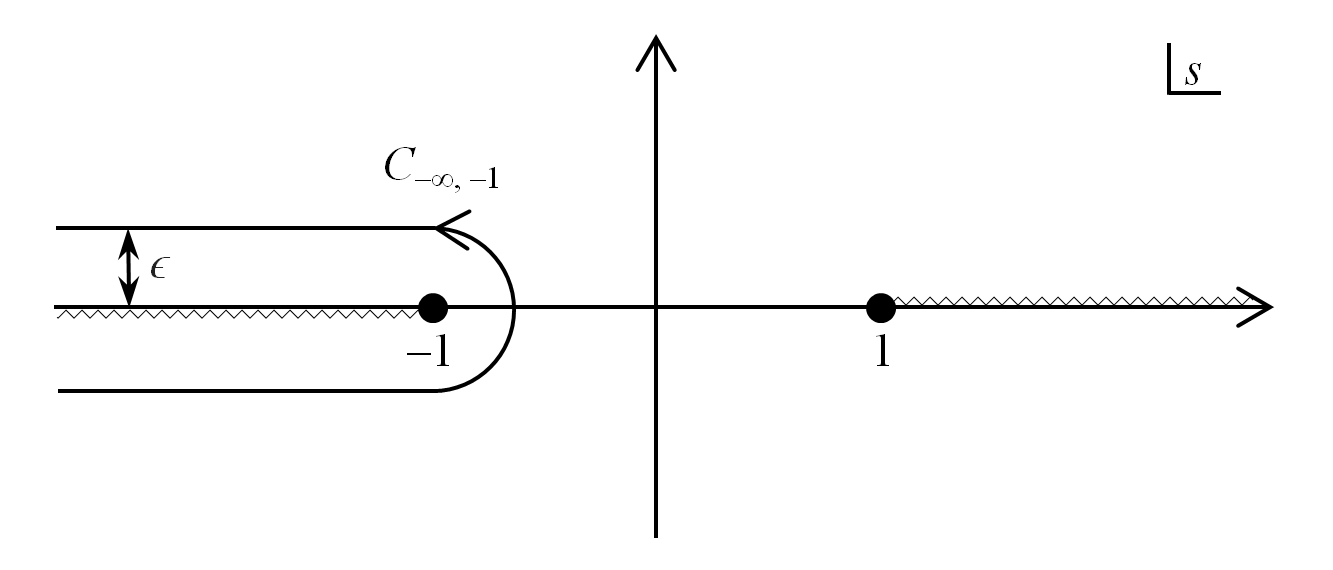
Figure 1:

Let us define the contour integral (Figure 1)

$$\oint_{C_{-\infty,-1}}=\int_{-\infty-i\epsilon}^{-1-i\epsilon}+\int_{-1-i\epsilon}^{-1+i\epsilon}+\int_{-1+i\epsilon}^{-\infty+i\epsilon}\text{ ,}$$ (3.3)

where $\epsilon$ is an infinitesimally small positive number, and $\int_{-1-i\epsilon}^{-1+i\epsilon}$ is a half-circle surrounding the right side of $-1$ on the complex plane. We adopt the branch cuts that are consistent with

$$\mathrm{Ln}\left(1-s\right)\text{\ \ \ and\ \ \ }\mathrm{Ln}\left(1+s\right)\text{ ,}$$ (3.4)

where $\mathrm{Ln}$ uses the principal branch of the phase angle $(-\pi,\pi]$ of its parameter. With this convention we can prove that

$$\int_{-\infty-i\epsilon}^{-1-i\epsilon}e^{2ws}\frac{\left(1-s\right)^{\lambda_{L}-\frac{1}{2}}}{\left(1+s\right)^{\lambda_{R}+\frac{1}{2}}}ds\overset{\epsilon\rightarrow 0}{=}\int_{-\infty}^{-1}e^{2ws}\frac{\left|s-1\right|^{\lambda_{L}-\frac{1}{2}}}{\left|s+1\right|^{\lambda_{R}+\frac{1}{2}}e^{-i\pi\left(\lambda_{R}+\frac{1}{2}\right)}}ds\text{ ,}$$

$$\int_{-1+i\epsilon}^{-\infty+i\epsilon}e^{2ws}\frac{\left(1-s\right)^{\lambda_{L}-\frac{1}{2}}}{\left(1+s\right)^{\lambda_{R}+\frac{1}{2}}}ds\overset{\epsilon\rightarrow 0}{=}\int_{-1}^{-\infty}e^{2ws}\frac{\left|s-1\right|^{\lambda_{L}-\frac{1}{2}}}{\left|s+1\right|^{\lambda_{R}+\frac{1}{2}}e^{i\pi\left(\lambda_{R}+\frac{1}{2}\right)}}ds\text{ .}$$ (3.5)

Furthermore, for the half-circle integral we can do a change of the variable $s=\epsilon e^{i\theta}-1$, then

$$\int_{-1-i\epsilon}^{-1+i\epsilon}e^{2ws}\frac{\left(1-s\right)^{\lambda_{L}-\frac{1}{2}}}{\left(1+s\right)^{\lambda_{R}+\frac{1}{2}}}ds=\int_{-\frac{\pi}{2}}^{\frac{\pi}{2}}e^{2w\left(\epsilon e^{i\theta}-1\right)}\frac{\left(2-\epsilon e^{i\theta}\right)^{\lambda_{L}-\frac{1}{2}}}{\left(\epsilon e^{i\theta}\right)^{\lambda_{R}+\frac{1}{2}}}i\epsilon e^{i\theta}d\theta\text{ ,}$$ (3.6)

which, by counting the power of $\epsilon$, obviously vanishes in the limit  $\epsilon\rightarrow 0$ when $\mathrm{Re}\left(\lambda_{R}\right)<\frac{1}{2}$. Therefore, using (3.5) and (3.2) we can derive

$$\oint_{C_{-\infty,-1}}e^{2ws}\frac{\left(1-s\right)^{\lambda_{L}-\frac{1}{2}}}{\left(1+s\right)^{\lambda_{R}+\frac{1}{2}}}ds$$ (3.7)

$$= 2^{1+\lambda_{L}-\lambda_{R}}i\cos\left(\pi\lambda_{R}\right)\Gamma\left(\frac{1}{2}-\lambda_{R}\right)e^{-2w}U\left(\frac{1}{2}-\lambda_{R},1+\lambda_{L}-\lambda_{R},4w\right)\text{ .}$$

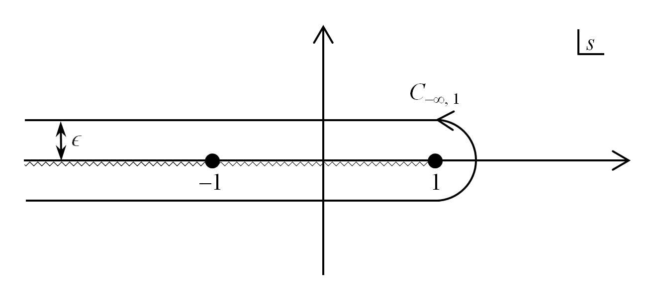
Figure 2:

Let us also define the contour integral (Figure 2)

$$\oint_{C_{-\infty,1}}=\int_{-\infty-i\epsilon}^{1-i\epsilon}+\int_{1-i\epsilon}^{1+i\epsilon}+\int_{1+i\epsilon}^{-\infty+i\epsilon}\text{ ,}$$ (3.8)

where $\int_{1-i\epsilon}^{1+i\epsilon}$ is a half-circle surrounding the right side of $1$ on the complex plane. Here we adopt the branch cuts that are consistent with

$$\mathrm{Ln}\left(s-1\right)\text{ \ \ and \ \ }\mathrm{Ln}\left(s+1\right)\text{ .}$$ (3.9)

Then we can derive

$$\int_{-\infty-i\epsilon}^{-1-i\epsilon}e^{2ws}\frac{\left(s-1\right)^{\lambda_{L}-\frac{1}{2}}}{\left(s+1\right)^{\lambda_{R}+\frac{1}{2}}}ds\overset{\epsilon\rightarrow 0}{=}\int_{-\infty}^{-1}e^{2ws}\frac{\left|s-1\right|^{\lambda_{L}-\frac{1}{2}}e^{-i\pi\left(\lambda_{L}-\frac{1}{2}\right)}}{\left|s+1\right|^{\lambda_{R}+\frac{1}{2}}e^{-i\pi\left(\lambda_{R}+\frac{1}{2}\right)}}ds\text{ ,}$$

$$\int_{-1-i\epsilon}^{1-i\epsilon}e^{2ws}\frac{\left(s-1\right)^{\lambda_{L}-\frac{1}{2}}}{\left(s+1\right)^{\lambda_{R}+\frac{1}{2}}}ds\overset{\epsilon\rightarrow 0}{=}\int_{-1}^{1}e^{2ws}\frac{\left|s-1\right|^{\lambda_{L}-\frac{1}{2}}e^{-i\pi\left(\lambda_{L}-\frac{1}{2}\right)}}{\left|s+1\right|^{\lambda_{R}+\frac{1}{2}}}ds\text{ ,}$$

$$\int_{-1-i\epsilon}^{1-i\epsilon}e^{2ws}\frac{\left(s-1\right)^{\lambda_{L}-\frac{1}{2}}}{\left(s+1\right)^{\lambda_{R}+\frac{1}{2}}}ds\overset{\epsilon\rightarrow 0}{=}\int_{-1}^{1}e^{2ws}\frac{\left|s-1\right|^{\lambda_{L}-\frac{1}{2}}e^{i\pi\left(\lambda_{L}-\frac{1}{2}\right)}}{\left|s+1\right|^{\lambda_{R}+\frac{1}{2}}}ds\text{ ,}$$

$$\int_{-1+i\epsilon}^{-\infty+i\epsilon}e^{2ws}\frac{\left(s-1\right)^{\lambda_{L}-\frac{1}{2}}}{\left(s+1\right)^{\lambda_{R}+\frac{1}{2}}}ds\overset{\epsilon\rightarrow 0}{=}\int_{-1}^{-\infty}e^{2ws}\frac{\left|s-1\right|^{\lambda_{L}-\frac{1}{2}}e^{i\pi\left(\lambda_{L}-\frac{1}{2}\right)}}{\left|s+1\right|^{\lambda_{R}+\frac{1}{2}}e^{i\pi\left(\lambda_{R}+\frac{1}{2}\right)}}ds\text{ .}$$ (3.10)

Again, we can see with a change of the variable $s=\epsilon e^{i\theta}+1$ that the half-circle integral

$$\int_{1-i\epsilon}^{1+i\epsilon}e^{2ws}\frac{\left(s-1\right)^{\lambda_{L}-\frac{1}{2}}}{\left(s+1\right)^{\lambda_{R}+\frac{1}{2}}}ds=\int_{-\frac{\pi}{2}}^{\frac{\pi}{2}}e^{2w\left(\epsilon e^{i\theta}+1\right)}\frac{\left(\epsilon e^{i\theta}\right)^{\lambda_{L}-\frac{1}{2}}}{\left(\epsilon e^{i\theta}+2\right)^{\lambda_{R}+\frac{1}{2}}}i\epsilon e^{i\theta}d\theta$$ (3.11)

vanishes in the limit $\epsilon\rightarrow 0$ when $\mathrm{Re}\left(\lambda_{L}\right)>-\frac{1}{2}$. Therefore, combining (3.10), (3.1) and (3.2) we can derive

$$\oint_{C_{-\infty,1}}e^{2ws}\frac{\left(s-1\right)^{\lambda_{L}-\frac{1}{2}}}{\left(s+1\right)^{\lambda_{R}+\frac{1}{2}}}ds = 2^{1+\lambda_{L}-\lambda_{R}}\pi i\cos\left(\pi\lambda_{L}\right)\sec\left(\pi\lambda_{R}\right)e^{-2w}L_{\lambda_{R}-\frac{1}{2}}^{\lambda_{L}-\lambda_{R}}\left(4w\right)$$

$$+2^{1+\lambda_{L}-\lambda_{R}}i\sin\left[\pi\left(\lambda_{L}-\lambda_{R}\right)\right]\Gamma\left(\frac{1}{2}-\lambda_{R}\right)e^{-2w}U\left(\frac{1}{2}-\lambda_{R},1+\lambda_{L}-\lambda_{R},4w\right)\text{ .}$$

The second term on the r.h.s. is the result of $\int_{-\infty-i\epsilon}^{-1-i\epsilon}+\int_{-1+i\epsilon}^{-\infty+i\epsilon}$, and it vanishes when $\lambda_{L}-\lambda_{R}\in\mathbb{Z}$, which can be explained by the cancellation of the branch cuts where $s<-1$ on the real-axis.

To summarize, we can rewrite the solution (2.10) as

$$f_{\lambda_{L}|\lambda_{R}}\left(a^{+},a^{-}\right)=\left(a^{+}\right)^{\lambda_{L}-\lambda_{R}}\left[\mathrm{C}_{5}\oint_{C_{-\infty,1}}e^{2ws}\frac{\left(s-1\right)^{\lambda_{L}-\frac{1}{2}}}{\left(s+1\right)^{\lambda_{R}+\frac{1}{2}}}ds+\mathrm{C}_{6}\oint_{C_{-\infty,-1}}e^{2ws}\frac{\left(1-s\right)^{\lambda_{L}-\frac{1}{2}}}{\left(1+s\right)^{\lambda_{R}+\frac{1}{2}}}\right]\text{ ,}$$ (3.13)

and it is important to notice that the convergence of the above contour integrals requires only Re$\left(w\right)>0$ and has no restrictions on $\lambda_{L,R}$. In the diagonal case $\lambda_{L}=\lambda_{R}$, due to the cancellation between two branch cuts, $\oint_{C_{-\infty,1}}$ can be replaced by $\oint_{C_{-1,1}}$, which is a contour integral surrounding the section of the real axis between $-1$ and $1$ (Figure 3).

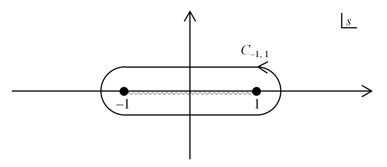
Figure 3:

At the end of this section, let us briefly compare the contours in this paper and the previous ones in [10, 16]. The stargenfunctions in [16] (or [10]) are just special cases in Section 2 with one (or two) of the left and right stargenvalues set to half-integers. Therefore, we should be able to reproduce these special cases also from the contour integrals. Take the first term on the r.h.s. of (3.13) for example, if we set $\lambda_{L}=\lambda_{R}\in\mathbb{Z+}\frac{1}{2}$, all brunch cuts can be dropped, then the contour reduces to two circles around the points $s=\pm 1$, one of which has zero residue, and thus the integral reproduces stargenfunctions with Laguerre polynomials as in [10]. Take the second term for another example, if we set $\lambda_{R}\mathbb{+}\frac{1}{2}\in\mathbb{Z}^{+}$, the left-side brunch cut in Figure 1 goes away, then the contour reduces to a circle around $s=-1$, and thus by keeping $\lambda_{L}\in$ $\mathbb{C}$ with the other brunch cut, the integral reproduces stargenfunctions with generalized Laguerre functions as in [16].

4 Creation and annihilation operators

The set of stargenfunctions (2.8) is the most direct generalization from [10, 16]. In this section, we investigate how they change by star-multiplying creation and/or annihilation operators to complex powers. Let us call the stargenfunctions represented by the two terms of (2.8), respectively, the “plus” and the “minus” branches. For convenience of star-product computation, we write the two branches by the integral representation (3.1), i.e.

$$f_{\lambda_{L}|\lambda_{R}}^{+}\left(a^{+},a^{-}\right) = \left(a^{+}\right)^{\lambda_{L}-\lambda_{R}}\int_{-1}^{1}e^{2ws}\frac{\left(1-s\right)^{\lambda_{L}-\frac{1}{2}}}{\left(1+s\right)^{\lambda_{R}+\frac{1}{2}}}ds\text{ ,}$$ (4.1a)

$$f_{\lambda_{L}|\lambda_{R}}^{-}\left(a^{+},a^{-}\right) = \left(a^{-}\right)^{\lambda_{R}-\lambda_{L}}\int_{-1}^{1}e^{2ws}\frac{\left(1-s\right)^{\lambda_{R}-\frac{1}{2}}}{\left(1+s\right)^{\lambda_{L}+\frac{1}{2}}}ds\text{ ,}$$ (4.1b)

where the constant overall factors have been dropped hereafter for simplicity. Note that the two branches are in general different, although they have the same stargenvalues, and that the two degenerate into one when $$\lambda_{R}-\lambda_{L}\in\mathbb{Z}$$ as already discussed around (2.11). In this section, we will investigate how these functions (as if they were eigenstates of the number operator in quantum mechanics) can be related by the creation and annihilation operators.

4.1 The plus and minus branches

We start from the diagonal case $\lambda_{L}=\lambda_{R}=\lambda$

$$f_{\lambda|\lambda}\left(a^{+},a^{-}\right)=\int_{-1}^{1}e^{2ws}\frac{\left(1-s\right)^{\lambda-\frac{1}{2}}}{\left(1+s\right)^{\lambda+\frac{1}{2}}}ds\text{ .}$$ (4.2)

We would like to show that by doing a left or a right star-product with $a^{\pm}$ to a complex power can shift the stargenvalue accordingly, and to this end we first express $a^{\pm}$ with the power $p$ using the Mellin transform (as done in [16])

$$\left(a^{\pm}\right)^{p}=\int_{0}^{+\infty}\frac{\tau^{-p-1}}{\Gamma\left(-p\right)}e^{-\tau a^{\pm}}d\tau\text{ ,}$$ (4.3)

so that we can pick out the factor $e^{-\tau a^{\pm}}$ for the convenience of doing star-products. Then by using (4.1), (4.3) and the following set of star-product results

$$e^{-\tau a^{+}}\star e^{2sw} = e^{2sw-\tau\left(1-s\right)a^{+}}\text{ ,}$$ (4.4a)

$$e^{-\tau a^{-}}\star e^{2sw} = e^{2sw-\tau\left(1+s\right)a^{-}}\text{ ,}$$ (4.4b)

$$e^{2sw}\star e^{-\tau a^{+}} = e^{2sw-\tau\left(1+s\right)a^{+}}\text{ ,}$$ (4.4c)

$$e^{2sw}\star e^{-\tau a^{-}} = e^{2sw-\tau\left(1-s\right)a^{-}}\text{ ,}$$ (4.4d)

we can easily prove that

$$f_{\lambda_{L}|\lambda_{R}}^{+} = \left(a^{+}\right)^{\lambda_{L}-\lambda_{R}}\star f_{\lambda_{R}|\lambda_{R}}=f_{\lambda_{L}|\lambda_{L}}\star\left(a^{+}\right)^{\lambda_{L}-\lambda_{R}}\text{ ,}$$ (4.5a)

$$f_{\lambda_{L}|\lambda_{R}}^{-} = \left(a^{-}\right)^{\lambda_{R}-\lambda_{L}}\star f_{\lambda_{R}|\lambda_{R}}=f_{\lambda_{L}|\lambda_{L}}\star\left(a^{-}\right)^{\lambda_{R}-\lambda_{L}}\text{ .}$$ (4.5b)

Thus the shift of the left (right) stargenvalue is indeed equal to the power of the creation (annihilation) operator acting from the left (right); or equal to the opposite power if it is the annihilation (creation) operator. Furthermore (4.5) shows that, starting from a diagonal stargenfunction, the creation / annihilation operator always brings it to the plus / minus branch, no matter whether the star-product is done from the left or from the right, and any non-diagonal stargenfunction of the two branches can be reached in this way, up to an overall constant, from a diagonal stargenfunction.

Naively we can further use $\left(a^{\pm}\right)^{p_{1}}\star\left(a^{\pm}\right)^{p_{2}}=\left(a^{\pm}\right)^{p_{1}+p_{2}}$ to conclude that the plus / minus branch is always closed under the star-multiplications with creation / annihilation operators to generic complex powers, but here we encounter some subtlety about associativity.

Star-products are not well-defined unless associativity holds, and associativity is bound to work if all the formulas to be star-multiplied are Taylor-expandable in the $Y$-coordinates. However, $a^{\pm}$ to complex powers cannot be Taylor-expanded. To circumvent the problem, we need to use integral representations, so that all the $a^{\pm}$’s stay in exponents, which makes the formulas Taylor-expandable. In other words, the integrals that we have used in this paper are not only technical tools to simplify the computation, but also very often the prescription to guarantee associativity. To ensure associativity during the computation, we need to keep in mind that all star-products should be computed before doing the integrals.

For example, in order to show

$$\left(a^{+}\right)^{p_{1}}\star\left(a^{+}\right)^{p_{2}}\star f_{\lambda|\lambda}=f_{\lambda+p_{1}+p_{2}|\lambda}^{+}\text{ ,}$$ (4.6)

we need to express all the factors by the integrals:

$$\left(a^{+}\right)^{p_{1}}\star\left(a^{+}\right)^{p_{2}}\star f_{\lambda|\lambda}$$ (4.7)

$$= \int_{0}^{+\infty}d\tau_{1}\int_{0}^{+\infty}d\tau_{2}\int_{-1}^{1}ds\frac{\tau_{1}^{-p_{1}-1}}{\Gamma\left(-p_{1}\right)}\frac{\tau_{2}^{-p_{2}-1}}{\Gamma\left(-p_{2}\right)}\frac{\left(1-s\right)^{\lambda-\frac{1}{2}}}{\left(1+s\right)^{\lambda+\frac{1}{2}}}e^{-\tau_{1}a^{+}}\star e^{-\tau_{2}a^{+}}\star e^{2ws}\text{ ,}$$

then we should do the integrals only after finishing the star-products within the integrand. By doing the star-products, the above formula equals

$$\int_{0}^{+\infty}d\tau_{1}\int_{0}^{+\infty}d\tau_{2}\int_{-1}^{1}ds\frac{\tau_{1}^{-p_{1}-1}}{\Gamma\left(-p_{1}\right)}\frac{\tau_{2}^{-p_{2}-1}}{\Gamma\left(-p_{2}\right)}\frac{\left(1-s\right)^{\lambda-\frac{1}{2}}}{\left(1+s\right)^{\lambda+\frac{1}{2}}}e^{2sw-\left(\tau_{1}+\tau_{2}\right)\left(1-s\right)a^{+}}\text{ ,}$$ (4.8)

and by rescaling $\tau_{1,2}$ it further equals

$$\int_{0}^{+\infty}d\tau_{1}\int_{0}^{+\infty}d\tau_{2}\int_{-1}^{1}ds\frac{\tau_{1}^{-p_{1}-1}}{\Gamma\left(-p_{1}\right)}\frac{\tau_{2}^{-p_{2}-1}}{\Gamma\left(-p_{2}\right)}\frac{\left(1-s\right)^{\lambda+p_{1}+p_{2}-\frac{1}{2}}}{\left(1+s\right)^{\lambda+\frac{1}{2}}}e^{2sw-\left(\tau_{1}+\tau_{2}\right)a^{+}}\text{ .}$$ (4.9)

In this way all star-products have been done between exponential functions of $Y$, thus the problem of associativity has been circumvented, and we can then do the integrals in (4.9), which gives $f_{\lambda+p_{1}+p_{2}|\lambda}^{+}$ as expected. Using this method we can prove that indeed the plus (minus) branch is closed by star-multiplications with arbitrarily many factors of creation (annihilation) operators.

4.2 Mixing the branches

Now naturally we want to ask the question: if both the creation and the annihilation operators together act on a stargenfunction, then what happens?

The first thing to check is whether the result is still a stargenfunction. As a test, we now examine whether

$$\left(a^{\mp}\right)^{\lambda^{\mp}}\star\left(a^{\pm}\right)^{\lambda^{\pm}}\star f_{\lambda|\lambda}$$ (4.10)

is a stargenfunction of $w$.

Using the lemma

$$e^{-\tau^{\mp}a^{\mp}}\star e^{-\tau^{\pm}a^{\pm}}\star e^{2sw}=e^{-\tau^{-}a^{-}\left(1+s\right)-\tau^{+}a^{+}\left(1-s\right)+\frac{1}{2}\left(\pm 1-s\right)\tau^{-}\tau^{+}+2sw}\text{ ,}$$ (4.11)

we obtain

$$\left(a^{\mp}\right)^{\lambda^{\mp}}\star\left(a^{\pm}\right)^{\lambda^{\pm}}\star f_{\lambda|\lambda}$$ (4.12)

$$= \int_{-1}^{1}ds\int_{0}^{+\infty}d\tau^{+}\int_{0}^{+\infty}d\tau^{-}\frac{\left(1-s\right)^{\lambda-\frac{1}{2}}}{\left(1+s\right)^{\lambda+\frac{1}{2}}}\frac{\left(\tau^{+}\right)^{-\lambda^{+}-1}}{\Gamma\left(-\lambda^{+}\right)}\frac{\left(\tau^{-}\right)^{-\lambda^{-}-1}}{\Gamma\left(-\lambda^{-}\right)}e^{2sw-\tau^{-}a^{-}\left(1+s\right)-\tau^{+}a^{+}\left(1-s\right)+\frac{1}{2}\left(\pm 1-s\right)\tau^{-}\tau^{+}}$$

$$= \int_{-1}^{1}ds\int_{0}^{+\infty}d\tau^{+}\int_{0}^{+\infty}d\tau^{-}\frac{\left(1-s\right)^{\lambda+\lambda^{+}-\frac{1}{2}}}{\left(1+s\right)^{\lambda-\lambda^{-}+\frac{1}{2}}}\frac{\left(\tau^{+}\right)^{-\lambda^{+}-1}}{\Gamma\left(-\lambda^{+}\right)}\frac{\left(\tau^{-}\right)^{-\lambda^{-}-1}}{\Gamma\left(-\lambda^{-}\right)}e^{2sw-\tau^{-}a^{-}-\tau^{+}a^{+}+\frac{\pm 1-s}{2\left(1-s^{2}\right)}\tau^{-}\tau^{+}}\text{ ,}$$

where in the last step we have simplified the formula by rescaling the integration variables $\tau^{\pm}$. We denote

$$g\left(\lambda,\lambda^{+},\lambda^{-},c\right)$$ (4.13)

$$= \int_{-1}^{1}ds\int_{0}^{+\infty}d\tau^{+}\int_{0}^{+\infty}d\tau^{-}\frac{\left(1-s\right)^{\lambda+\lambda^{+}-\frac{1}{2}}}{\left(1+s\right)^{\lambda-\lambda^{-}+\frac{1}{2}}}\frac{\left(\tau^{+}\right)^{-\lambda^{+}-1}}{\Gamma\left(-\lambda^{+}\right)}\frac{\left(\tau^{-}\right)^{-\lambda^{-}-1}}{\Gamma\left(-\lambda^{-}\right)}e^{2sw-\tau^{-}a^{-}-\tau^{+}a^{+}-\frac{c+s}{2\left(1-s^{2}\right)}\tau^{-}\tau^{+}}\text{ .}$$

For convergence, we restrict Re$\left(\lambda\pm\lambda^{\pm}\right)<\frac{1}{2}$, Re$\left(\lambda^{\pm}\right)<0$ and Re$\left(c\right)>1$, and (4.10) is restored by analytically continuing $g\left(\lambda,\lambda^{+},\lambda^{-},c\right)$ and setting $c=\mp 1$. We can prove that (4.10) is still a stargenfunction of $w$, if we can prove

$$w\star g\left(\lambda,\lambda^{+},\lambda^{-},c\right) = \left(\lambda+\lambda^{+}-\lambda^{-}\right)g\left(\lambda,\lambda^{+},\lambda^{-},c\right)\text{ ,}$$ (4.14)

$$g\left(\lambda,\lambda^{+},\lambda^{-},c\right)\star w = \lambda g\left(\lambda,\lambda^{+},\lambda^{-},c\right)\text{ .}$$ (4.15)

To this end, there is no need to perform the integrals of (4.13), we only need to use its integrand to read out the stargenvalues.

In the same way as deriving (2.2a), we convert the $w\star$ on the l.h.s. of (4.14) into derivatives w.r.t. $a^{\pm}$ and hence obtain

$$w\star e^{2sw-\tau^{-}a^{-}-\tau^{+}a^{+}}$$ (4.16)

$$= \left[-\frac{s}{2}+w\left(1-s^{2}\right)-\frac{1}{2}\tau^{+}a^{+}\left(1-s\right)+\frac{1}{2}\tau^{-}a^{-}\left(1+s\right)-\frac{1}{4}\tau^{+}\tau^{-}\right]e^{2sw-\tau^{-}a^{-}-\tau^{+}a^{+}}\text{ ,}$$

which leads to

$$w\star g\left(\lambda,\lambda^{+},\lambda^{-},c\right)$$

$$= \int_{-1}^{1}ds\int_{0}^{+\infty}d\tau^{+}\int_{0}^{+\infty}d\tau^{-}\frac{\left(1-s\right)^{\lambda+\lambda^{+}-\frac{1}{2}}}{\left(1+s\right)^{\lambda-\lambda^{-}+\frac{1}{2}}}\frac{\left(\tau^{+}\right)^{-\lambda^{+}-1}}{\Gamma\left(-\lambda^{+}\right)}\frac{\left(\tau^{-}\right)^{-\lambda^{-}-1}}{\Gamma\left(-\lambda^{-}\right)}e^{2sw-\tau^{-}a^{-}-\tau^{+}a^{+}-\frac{c+s}{2\left(1-s^{2}\right)}\tau^{-}\tau^{+}}$$

$$\ \ \ \ \left[-\frac{s}{2}+w\left(1-s^{2}\right)-\frac{1}{2}\tau^{+}a^{+}\left(1-s\right)+\frac{1}{2}\tau^{-}a^{-}\left(1+s\right)-\frac{1}{4}\tau^{+}\tau^{-}\right]$$

$$= \int_{-1}^{1}ds\int_{0}^{+\infty}d\tau^{+}\int_{0}^{+\infty}d\tau^{-}\frac{\left(1-s\right)^{\lambda+\lambda^{+}-\frac{1}{2}}}{\left(1+s\right)^{\lambda-\lambda^{-}+\frac{1}{2}}}\frac{\left(\tau^{+}\right)^{-\lambda^{+}-1}}{\Gamma\left(-\lambda^{+}\right)}\frac{\left(\tau^{-}\right)^{-\lambda^{-}-1}}{\Gamma\left(-\lambda^{-}\right)}e^{2sw-\tau^{-}a^{-}-\tau^{+}a^{+}-\frac{c+s}{2\left(1-s^{2}\right)}\tau^{-}\tau^{+}}$$ (4.17d)

$$\ \ \ \ \left\{e^{-2sw}\left[-\frac{s}{2}+\frac{1}{2}\left(1-s^{2}\right)\frac{\partial}{\partial s}\right]e^{2sw}\right.$$

$$\ \ \ \ \left.+e^{\tau^{+}a^{+}}\left[\frac{1}{2}\tau^{+}\left(1-s\right)\frac{\partial}{\partial\tau^{+}}\right]e^{-\tau^{+}a^{+}}\right.$$

$$\ \ \ \ \left.+e^{\tau^{-}a^{-}}\left[-\frac{1}{2}\tau^{-}\left(1+s\right)\frac{\partial}{\partial\tau^{-}}\right]e^{-\tau^{-}a^{-}}\right.$$

$$\ \ \ \ \left.-\frac{1}{4}\tau^{+}\tau^{-}\right\}\text{ .}$$

We can convert the terms (4.17d) (4.17d) and (4.17d) by integrations by parts, so that the curly bracket above can be replaced with

$$\ \ \ \left\{\left[\lambda+\frac{1}{2}\left(1+s\right)\lambda^{+}-\frac{1}{2}\left(1-s\right)\lambda^{-}+\frac{1+2cs+s^{2}}{4\left(1-s^{2}\right)}\tau^{+}\tau^{-}\right]\right.\$$

$$\ \ \ \ \left.+\left[\frac{1}{2}\left(1-s\right)\lambda^{+}+\frac{c+s}{4\left(1+s\right)}\tau^{+}\tau^{-}\right]\right.$$

$$\ \ \ \ \left.+\left[-\frac{1}{2}\left(1+s\right)\lambda^{-}-\frac{c+s}{4\left(1-s\right)}\tau^{+}\tau^{-}\right]\right.$$

$$\ \ \ \ \left.-\frac{1}{4}\tau^{+}\tau^{-}\right\}\text{ ,}$$

which is exactly equal to the factor $\left(\lambda+\lambda^{+}-\lambda^{-}\right)$, and thus (4.14) is proven. Moreover (4.15) can also be proven in the same manner, whose details we will skip.

In (4.10), we can use (4.5) to move one or both of the creation and annihilation factors to the right side, and thus it is clear that a diagonal stargenfunction of the type (2.8), star-multiplied with two factors respectively of creation and annihilation operators to arbitrary complex powers, gives a new stargenfunction with the expected stargenvalues. The new stargenfunction in general should be a linear combination of different branches, but we are not yet able to decompose it. What makes the problem more complicated is that, when the plus and minus branches degenerate, there exists an extra branch of stargenfunctions. Such an extra branch is very likely to be activated by some combinations of creation and annihilation operators. To illustrate this, in (4.10) we set $\lambda^{+}=\lambda^{-}=\tilde{\lambda}$, which leads to a diagonal stargenfunction, and by performing the $\tau^{\pm}$ integrals in (4.13) we get

$$g\left(\lambda,\tilde{\lambda},\tilde{\lambda},c\right)$$ (4.18)

$$= \int_{-1}^{1}ds\ 2^{-\tilde{\lambda}}\frac{\left(1-s\right)^{\lambda-\frac{1}{2}+\tilde{\lambda}}}{\left(1+s\right)^{\lambda+\frac{1}{2}-\tilde{\lambda}}}\left(\frac{c+s}{1-s^{2}}\right)^{\tilde{\lambda}}e^{2sw}U\left(-\tilde{\lambda},1,\frac{2\left(1-s^{2}\right)}{c+s}w\right)\text{ .}$$

Note that the extra branch can be represented (except for the special cases with half-integer stargenvalues) by the second term in (2.10), which contains a factor $U\left(\frac{1}{2}-\lambda,1,4w\right)$ that logarithmically diverges as $w\rightarrow 0$. In (4.18), we can find a similar factor $U\left(-\tilde{\lambda},1,\frac{2\left(1-s^{2}\right)}{c+s}w\right)$ whose expansion w.r.t. $w$ also gives $\log w$, and we therefore speculate that the extra branch is involved.

5 Conclusion and discussion

In this paper, motivated by the construction of initial data in the holomorphic gauge to solve Vasiliev’s equations, we have studied the stargenfunctions of the number operator, as defined in (1.11) with generic complex stargenvalues. We have re-written these stargenfunctions using integral representations and also expressed the creation and annihilation operators to complex powers by integrals via the Mellin transform, so that their star-products can be computed conveniently. We have in particular picked out a set of stargenfunctions (2.8) to investigate how they are changed by creation and annihilation operators. This set of stargenfunctions can be written as linear combinations of two subsets of stargenfunctions (the “plus” and “minus” branches), except that the two subsets intersect when left and the right stargenvalues differ by an integer. The whole plus (minus) branch of stargenfunctions can be related (up to overall constants) by – and is closed under – the star-multiplications with creation (annihilation) operators to generic complex powers. However, by mixing the usage of creation and annihilation operators, (2.8) does not seem to close, although the stargenvalues are likely to be what we expect. We have confirmed that a diagonal stargenfunction of the type (2.8), star-multiplied by two factors respectively of creation and annihilation operators to complex powers, yields another stargenfunction with the expected stargenvalues. We speculate that the resulting stargenfunction should be a linear combination of the plus and minus branches when they are non-degenerate and that another extra branch should be involved in the degenerate case.

We are not yet able to use the above results to construct valid solutions to Vasiliev’s equations. One of the difficulties happens when we go beyond linear combinations of the stargenfunctions. As in (1.8) the twistor space gauge field $V^{\prime}$ is expressed in terms of star-product series of the initial-data field $\Psi$. Thus, for example if we use the stargenfunctions $f_{\lambda_{L}|\lambda_{R}}^{\pm}$ above to construct $\Psi$, we will encounter star-multiplications to all orders between these stargenfunctions, and we have to make sure that such star-multiplications make sense. Let us take a look at the diagonal stargenfunctions to illustrate the problem. When the stargenvalues are half-integers, according to [10], $f_{\lambda|\lambda}$ should act like a projector: $f_{\lambda_{1}|\lambda_{1}}\star f_{\lambda_{2}|\lambda_{2}}\propto\delta_{\lambda_{1}\lambda_{2}}f_{\lambda_{2}|\lambda_{2}}$. Naively we expect the same thing to happen for generic complex stargenvalues, which however, does not seem to be true.

If we multiply the expression (4.2) by itself, by using the lemma

$$e^{2sw}\star e^{2s^{\prime}w}=\frac{1}{1+ss^{\prime}}e^{2\frac{s+s^{\prime}}{1+ss^{\prime}}w}\text{ ,}$$ (5.1)

and denoting $\Delta\lambda\equiv\lambda_{1}-\lambda_{2}$, we get

$$f_{\lambda_{1}|\lambda_{1}}\star f_{\lambda_{2}|\lambda_{2}}$$ (5.2)

$$= \int_{-1}^{1}\int_{-1}^{1}ds\ ds^{\prime}\ e^{2ws}\frac{\left(1-s\right)^{\lambda_{1}-\frac{1}{2}}}{\left(1+s\right)^{\lambda_{1}+\frac{1}{2}}}\frac{\left(1-s^{\prime}\right)^{\lambda_{2}-\frac{1}{2}}}{\left(1+s^{\prime}\right)^{\lambda_{2}+\frac{1}{2}}}\frac{1}{1+ss^{\prime}}e^{2\frac{s+s^{\prime}}{1+ss^{\prime}}w}$$

$$= \int_{-1}^{1}ds\frac{\left(1-s\right)^{\Delta\lambda-1}}{\left(1+s\right)^{\Delta\lambda+1}}\int_{-1}^{1}\ du\ \frac{\left(1-u\right)^{\lambda_{2}-\frac{1}{2}}}{\left(1+u\right)^{\lambda_{2}+\frac{1}{2}}}e^{2uw}$$

$$= f_{\lambda_{2}|\lambda_{2}}\int_{-1}^{1}ds\frac{\left(1-s\right)^{\Delta\lambda-1}}{\left(1+s\right)^{\Delta\lambda+1}}\text{ ,}$$

where in the second last step the integration variable $s^{\prime}$ has been changed by $s^{\prime}=\frac{s-u}{su-1}$ or equivalently $u=\frac{s+s^{\prime}}{1+ss^{\prime}}$. In the last line of (5.2), obviously the integral is problematic: let $\epsilon$ be a small positive number, then we have

$$\int_{-1+\epsilon}^{1-\epsilon}ds\frac{\left(1-s\right)^{\Delta\lambda-1}}{\left(1+s\right)^{\Delta\lambda+1}}=\frac{1}{2\Delta\lambda}\left[\left(\frac{2-\epsilon}{\epsilon}\right)^{\Delta\lambda}-\left(\frac{\epsilon}{2-\epsilon}\right)^{\Delta\lambda}\right]\text{ ,}$$ (5.3)

and as the factors $\epsilon^{-\Delta\lambda}$ and $\epsilon^{\Delta\lambda}$ indicate, if $\epsilon$ is set to $0$, for any $\Delta\lambda$ the integral does not converge.

In the paper [10] for half-integer stargenvalues, a prescription has been given: the real-axis integral $\int_{-1}^{1}$ has been replaced with the contour integral around either $s=1$ or $s=-1$ (both types of integrals can produce the same Laguerre polynomial at the beginning). In that case, while the real-axis integral is problematic, the contour one converges and leads to the expected projector result. On the contrary, in this paper for complex stargenvalues, we have to prescribe with a different contour $C_{-1,1}$ as shown in Figure 3, i.e. we now have the factor:

$$\oint_{C_{-1,1}}ds\frac{\left(s-1\right)^{\Delta\lambda-1}}{\left(s+1\right)^{\Delta\lambda+1}}$$ (5.4)

in the prescribed result of $f_{\lambda_{1}|\lambda_{1}}\star f_{\lambda_{2}|\lambda_{2}}$. For $\Delta\lambda\neq 0$, we can do the indefinite integral:

$$\int ds\frac{\left(s-1\right)^{\Delta\lambda-1}}{\left(s+1\right)^{\Delta\lambda+1}}=\frac{1}{2\Delta\lambda}\left(\frac{s-1}{s+1}\right)^{\Delta\lambda}+\ \text{const. .}$$ (5.5)

Within a given branch of the function on the r.h.s. of (5.5), by going through a full cycle along the contour $C_{-1,1}$, both $\left(s-1\right)$ and $\left(s+1\right)$ acquire the same phase factors that cancel each other, i.e. the value of the primitive function is not changed by a full cycle along $C_{-1,1}$. Therefore, the integral (5.4) gives 0. For the special case $\Delta\lambda=0$, (5.4) becomes the sum of two cancelling residues around $s=1$ and $-1$, which also gives 0. Therefore, with such a prescription, $f_{\lambda_{1}|\lambda_{1}}\star f_{\lambda_{2}|\lambda_{2}}=0$ always holds, even if $\lambda_{1}=\lambda_{2}$. It is not yet certain to us how this should be interpreted – perhaps we should for consistency exclude half-integer stargenvalues when we use such stargenfunctions to construct the initial data, or perhaps we should find a better prescription that we are not yet aware of.

Another complication is the star-product with the inner Klein operators. As introduced around (1.12), to construct the initial data, we need to make two copies of the stargenfunctions. If each copy has two branches e.g. ($+,-$), then two copies give four branches ($++,+-,-+,--$) in the initial data. A stargenfunction of any particular branch star-multiplied by $\kappa_{y}$ or $\bar{\kappa}_{\bar{y}}$ in general may lead to combinations of all branches. Thus the computation is very much involved, and we will continue these investigations in our future work.

Acknowledgement   This work is supported by “the Fundamental Research Funds for the Central Universities, NO. NS2020054” of China. The author would like to thank R. Aros, D. De Filippi, V.E. Didenko, C. Iazeolla, P. Sundell and the anonymous referee for inspiring discussions. In particular, the author is grateful to C. Iazeolla and P. Sundell for pointing out important details about the contour integrals. The author would also like to thank all the organizers and hosts of the APCTP-KHU Workshop on Higher Spin Gravity in Pohang, South Korea, for hospitality and for providing this excellent opportunity for discussions that helped the improvement of this paper.

References

- [1] M. A. Vasiliev, “Consistent equation for interacting gauge fields of all spins in (3+1)-dimensions,” Phys. Lett. B243 (1990) 378–382.
- [2] M. A. Vasiliev, “Higher spin gauge theories: Star product and AdS space,” arXiv:hep-th/9910096 [hep-th].
- [3] C. Fronsdal, “Massless Fields with Integer Spin,” Phys. Rev. D18 (1978) 3624.
- [4] J. Fang and C. Fronsdal, “Massless Fields with Half Integral Spin,” Phys. Rev. D18 (1978) 3630.
- [5] E. Sezgin and P. Sundell, “An Exact solution of 4-D higher-spin gauge theory,” Nucl. Phys. B762 (2007) 1–37, arXiv:hep-th/0508158 [hep-th].
- [6] C. Iazeolla, E. Sezgin, and P. Sundell, “Real forms of complex higher spin field equations and new exact solutions,” Nucl. Phys. B791 (2008) 231–264, arXiv:0706.2983 [hep-th].
- [7] V. E. Didenko and M. A. Vasiliev, “Static BPS black hole in 4d higher-spin gauge theory,” Phys. Lett. B682 (2009) 305–315, arXiv:0906.3898 [hep-th]. [Erratum: Phys. Lett.B722,389(2013)].
- [8] C. Iazeolla and P. Sundell, “4D Higher Spin Black Holes with Nonlinear Scalar Fluctuations,” JHEP 10 (2017) 130, arXiv:1705.06713 [hep-th].
- [9] C. Iazeolla, E. Sezgin, and P. Sundell, “On Exact Solutions and Perturbative Schemes in Higher Spin Theory,” Universe 4 no. 1, (2018) 5, arXiv:1711.03550 [hep-th].
- [10] C. Iazeolla and P. Sundell, “Families of exact solutions to Vasiliev’s 4D equations with spherical, cylindrical and biaxial symmetry,” JHEP 12 (2011) 084, arXiv:1107.1217 [hep-th].
- [11] C. Iazeolla and P. Sundell, “Biaxially symmetric solutions to 4D higher-spin gravity,” J. Phys. A46 (2013) 214004, arXiv:1208.4077 [hep-th].
- [12] S. S. Gubser and W. Song, “An axial gauge ansatz for higher spin theories,” JHEP 11 (2014) 036, arXiv:1405.7045 [hep-th].
- [13] J. Bourdier and N. Drukker, “On Classical Solutions of 4d Supersymmetric Higher Spin Theory,” JHEP 04 (2015) 097, arXiv:1411.7037 [hep-th].
- [14] P. Sundell and Y. Yin, “New classes of bi-axially symmetric solutions to four-dimensional Vasiliev higher spin gravity,” JHEP 01 (2017) 043, arXiv:1610.03449 [hep-th].
- [15] R. Aros, C. Iazeolla, J. Noreña, E. Sezgin, P. Sundell, and Y. Yin, “FRW and domain walls in higher spin gravity,” JHEP 03 (2018) 153, arXiv:1712.02401 [hep-th].
- [16] R. Aros, C. Iazeolla, P. Sundell, and Y. Yin, “Higher spin fluctuations on spinless 4D BTZ black hole,” JHEP 08 (2019) 171, arXiv:1903.01399 [hep-th].
- [17] S. F. Prokushkin and M. A. Vasiliev, “Higher spin gauge interactions for massive matter fields in 3-D AdS space-time,” Nucl. Phys. B545 (1999) 385, arXiv:hep-th/9806236 [hep-th].
- [18] V. E. Didenko, A. S. Matveev, and M. A. Vasiliev, “BTZ Black Hole as Solution of 3-D Higher Spin Gauge Theory,” Theor. Math. Phys. 153 (2007) 1487–1510, arXiv:hep-th/0612161 [hep-th]. [Teor. Mat. Fiz.153,158(2007)].
- [19] C. Iazeolla and J. Raeymaekers, “On big crunch solutions in Prokushkin-Vasiliev theory,” JHEP 01 (2016) 177, arXiv:1510.08835 [hep-th].
- [20] M. A. Vasiliev, “Algebraic aspects of the higher spin problem,” Phys. Lett. B257 (1991) 111–118.
- [21] D. De Filippi, C. Iazeolla, and P. Sundell, “Fronsdal fields from gauge functions in Vasiliev’s higher spin gravity,” JHEP 10 (2019) 215, arXiv:1905.06325 [hep-th].
- [22] M. Banados, C. Teitelboim, and J. Zanelli, “The black hole in three-dimensional space-time,” Phys. Rev. Lett. 69 (1992) 1849–1851, hep-th/9204099.
- [23] M. Banados, M. Henneaux, C. Teitelboim, and J. Zanelli, “Geometry of the (2+1) black hole,” Phys. Rev. D48 (1993) 1506–1525, arXiv:gr-qc/9302012 [gr-qc]. [Erratum: Phys. Rev.D88,069902(2013)].
- [24] S. Aminneborg, I. Bengtsson, S. Holst, and P. Peldan, “Making anti-de Sitter black holes,” Class. Quant. Grav. 13 (1996) 2707–2714, arXiv:gr-qc/9604005 [gr-qc].
- [25] S. Holst and P. Peldan, “Black holes and causal structure in anti-de Sitter isometric space-times,” Class. Quant. Grav. 14 (1997) 3433–3452, arXiv:gr-qc/9705067 [gr-qc].
- [26] M. Banados, A. Gomberoff, and C. Martinez, “Anti-de sitter space and black holes,” Class. Quant. Grav. 15 (1998) 3575, hep-th/9805087.
- [27] C. Iazeolla and P. Sundell, “A Fiber Approach to Harmonic Analysis of Unfolded Higher-Spin Field Equations,” JHEP 10 (2008) 022, arXiv:0806.1942 [hep-th].