Sequential Training of Neural Networks with Gradient Boosting

Abstract

This paper presents a novel technique based on gradient boosting to train the final layers of a neural network (NN). Gradient boosting is an additive expansion algorithm in which a series of models are trained sequentially to approximate a given function. A neural network can also be seen as an additive expansion where the scalar product of the responses of the last hidden layer and its weights provide the final output of the network. Instead of training the network as a whole, the proposed algorithm trains the network sequentially in $T$ steps. First, the bias term of the network is initialized with a constant approximation that minimizes the average loss of the data. Then, at each step, a portion of the network, composed of $J$ neurons, is trained to approximate the pseudo-residuals on the training data computed from the previous iterations. Finally, the $T$ partial models and bias are integrated as a single NN with $T\times J$ neurons in the hidden layer. Extensive experiments in classification and regression tasks, as well as in combination with deep neural networks, are carried out showing a competitive generalization performance with respect to neural networks trained with different standard solvers, such as Adam, L-BFGS, SGD and deep models. Furthermore, we show that the proposed method design permits to switch off a number of hidden units during test (the units that were last trained) without a significant reduction of its generalization ability. This permits the adaptation of the model to different classification speed requirements on the fly.

1 Introduction

Machine learning is becoming a fundamental piece for the success of more and more applications every day. Some examples of novel applications include bioactive molecule prediction [1], renewable energy prediction [41], classification of galactic sources [31], or agriculture area for mapping soil contamination [24]. It is of capital importance to find algorithms that can efficiently handle complex data. Ensemble methods are very effective at improving the generalization accuracy of multiple simple models [16, 7] or even complex models such as MLPs [38] or DeepCNNs [32].

In recent years, gradient boosting [19, 18], a fairly old technique has gained much attention, specially due to the novel and computationally efficient version of gradient boosting called eXtreme Gradient Boosting or XGBoost [9]. Gradient boosting builds a model as an additive expansion of regressors to gradually minimize a given loss function. When gradient boosting is combined with several stochastic techniques, as bootstrapping or feature sampling from random forest [6], its performance generally improves [20]. In fact, this combination of randomization techniques and optimization has placed XGBoost among the top contenders in Kaggle competitions [9] and provides excellent performance in a variety of applications as in the ones mentioned above. Based on the success of XGBoost, other techniques have been proposed like CatBoost [35] and LightGBM [25], which propose improvements in training speed and generalization performance. More details about these methods can be seen in the comparative analysis of Bentéjac et al. [3]. Other type of widespread boosting algorithm is AdaBoost [17], initially developed for binary classification and then for multi-class classification (AdaBoost-SAMME) [21] and regression [15].

On the other hand, convolutional deep architectures have shown outstanding performances especially with structured data such as images, speech, etc. [28, 37]. However, in the context of tabular data, ensembles of classifiers or simple MLPs are generally more effective than convolutional deep neural networks [43]. The objective of this study is to combine the stage-wise optimization of gradient boosting into the training procedure of the last layers of a neural network. The result of the proposed algorithm is an alternative for training a single neural network (not an ensemble of networks).

Several related studies propose hybrid algorithms that, for instance, transform a decision forest into a single neural network [42, 4] or that use a deep architecture to train a tree forest [26]. In [42], it is shown that a pre-trained tree forest can be cast into a two-layer neural network with the same predictive outputs. First, each tree is converted into a neural network. To do so, each split in the tree is transformed into an individual neuron that is connected to a single input attribute (split attribute) and whose activation threshold is set to the split threshold. In this way, and by a proper combination of the outputs of these neurons (splits) the network mimics the behavior of the decision tree. Finally, all neurons are combined through a second layer, which recovers the forest decision. The weights of this network can be later retrained to obtain further improvements [4]. In [26], a decision forest is trained jointly by means of a deep neural network that learns all splits of all trees of the forest. To guide the network to learn the splits of the trees, a procedure that trains the trees using back-propagation, is proposed. The final output of the algorithm is a decision forest whose performance is remarkable in image classification tasks.

In other related line of work [33, 23], boosting is applied to the construction of Deep Residual Learning models [22]. In [33], a novel ResNet weight estimation model is proposed by generalizing the boosting functional gradient minimization [30] to the feature extraction space of the network. The work presented in [23] also builds layer-by-layer a ResNet boosting over features, however, it is based on a different boosting framework [17]. The model (called BoostResNet) works by learning a linear classifier on the output of each residual network block to build an ensemble of shallow blocks. One important advantage of BoostResNet over standard ResNet is its lower computational complexity although the reported performance is not consistently better with respect to ResNet. In contrast, the current proposal method, based on [19], builds a simple shallow network in-width rather than complex model in-depth and shows very good performance in tabular datasets with respect to standard back-propagation training methods. Furthermore, our proposal can adapt on the fly to the use of a reduced number of hidden neurons.

Another model that resembles the idea proposed in this paper –yet with a different optimization process, final model and objective– was presented in [2]. They propose a convex optimization algorithm for training a neural network that theoreticallly could reach the global optimum although its exact implementation is only feasible for a very low number of input features. In order to reach the global optimum they control the number of hidden neurons of the model by adding one neuron at a time to the network and by including a $L^{1}$ regularization on the top layer. The proposed idea is a stepwise algorithm as all weights of the network are optimized at each iteration. This is done in three optimization steps. First, a new neuron (i.e. linear model) is added and trained on a weighted loss function similarly to Adaboost. This weighted loss can only be solved exactly for a very low number of input features. Then, the output layer, and potentially all input weights, are optimized using the proposed convex formulation. Finally, the output weights are regularized to reduce the complexity of the network. This final step sets to zero some of the output weights to effectively remove the corresponding neurons. The algorithm is tested on one simple 2D problem in order to assess the validity of the global optimum approach.

In this paper, we propose a combination of ensembles and neural networks that is somehow complementary to the work of [26], which is a single neural network that is trained using an ensemble training algorithm. Specifically, we propose to train a neural network iteratively as an additive expansion of simpler models. The algorithm is equivalent to gradient boosting: first, a constant approximation is computed (assigned to the bias term of the neural network), then at each step, a regression neural network with a single (or very few) neuron(s) in the hidden layer is trained to fit the residuals of the previous models. All these models are then combined to form a single neural network with one hidden layer. This training procedure provides an alternative to standard training solvers (such as Adam, L-BFGS or SGD) for training a neural network. Other works related to the optimization and convergence of Adam have been recently proposed [36, 11, 8]. They showed that its convergence can be improved in the context of high dimensional complex image classification tasks. However, their focus is mainly in deep models for image classification tasks.

In addition, the proposed method has an additive neural architecture in which the latest computed neurons contribute less to the final decision. This can be useful in computationally intensive applications as the number of active models (or neurons) can be gauged on the fly to the available computational resources without a significant loss in generalization accuracy. The proposed model is tested on multiple classification and regression problems, as well as in conjunction with deep models posed as transfer learning problems. These experiments show that the proposed method for training the last layers of a neural network is a good alternative to other standard methods.

The paper is organized as follows: Section 2 describes gradient boosting and how to apply it to train a single neural network; In section 3 the results of several experimental analysis are shown; Finally, the conclusions are summarized in the last section.

2 Methodology

In this section, we show the gradient boosting mathematical framework [19] and the applied modifications in order to use it for training a neural network sequentially. The proposed algorithm is valid for multi-class and binary classification, and for regression. Finally, an illustrative example is given.

2.1 Gradient boosting

Given a training dataset $D=\{\mathbf{x}_{i},y_{i}\}_{1}^{N}$, the goal of machine learning algorithms is to find an approximation, $\hat{F}(\mathbf{x})$, of the objective function $F^{*}(\mathbf{x})$, which maps instances $\mathbf{x}$ to their output values $y$. In general, the learning process can be posed as an optimization problem in which the expected value of a given loss function, $\mathds{E}[L(y,F(\mathbf{x}))]$, is minimized. A data-based estimate can be used to approximate this expected loss: $\sum_{i=1}^{N}L(y_{i},F(\mathbf{x}_{i}))$.

In the specific case of gradient boosting, the model is built using an additive expansion

$$F_{t}(\mathbf{x})=F_{t-1}(\mathbf{x})+\rho_{t}h_{t}(\mathbf{x}),$$ (1)

where $\rho_{t}$ is the weight of the $t^{th}$ function, $h_{t}(\mathbf{x})$. The approximation is constructed stage-wise in the sense that at each step, a new model $h_{t}$ is built without modifying any of the previously created models included in $F_{t-1}(\mathbf{x})$. First, the additive expansion is initialized with a constant approximation

$$F_{0}(\mathbf{x})=\operatorname*{\arg\!\min}_{\alpha}\sum_{i=1}^{N}L(y_{i},\alpha)\;$$ (2)

and the following models are built in order to minimize

$$(\rho_{t},h_{t}(\mathbf{x}))=\operatorname*{\arg\!\min}_{\rho,h_{t}}\sum_{i=1}^{N}L(y_{i},F_{t-1}(\mathbf{x}_{i})+\rho h_{t}(\mathbf{x}_{i}))\;\;.$$ (3)

However, instead of jointly solve the optimization for $\rho$ and $h_{t}$, the problem is split into two steps. First, each model $h_{t}$ is trained to learn the data-based gradient vector of the loss-function. For that, each model, $h_{t}$, is trained on a new dataset $D=\{\mathbf{x}_{i},r_{ti}\}_{i=1}^{N}$, where the pseudo-residuals, $r_{ti}$, are the negative gradient of the loss function at $F_{t-1(\mathbf{x_{i}})}$

$$r_{ti}=\left.-\frac{\partial L(y_{i},F(\mathbf{x}_{i}))}{\partial F(\mathbf{x}_{i})}\right|_{F(\mathbf{x})=F_{t-1}(\mathbf{x})}$$ (4)

The function, $h_{t}$, is expected to output values close to the pseudo residuals at the given data points, which are parallel to the gradient of $L$ at $F_{t-1}(\mathbf{x})$. Note, however, that the training process of $h$ is generally guided by square-error loss, which may be different from the given objective loss function. Notwithstanding, the value of $\rho_{t}$ is subsequently computed by solving a line search optimization problem on the given loss function

$$\rho_{t}=\operatorname*{\arg\!\min}_{\rho}\sum_{i=1}^{N}L(y_{i},F_{t-1}(\mathbf{x}_{i})+\rho h_{t}(\mathbf{x}_{i}))\;\;.$$ (5)

The original formulation of gradient boosting (as given in [19]) is, in some final derivations, only valid for decision trees. Here, we present an extension of the formulation of gradient boosting to be able to use any possible regressor as base model and we describe how to integrate this process to train a single neural network, which is the focus of the paper.

2.2 Binary classification

For binary classification, in which $y\in\{-1,1\}$, we will consider the logistic loss

$$L(y,F(\cdot))=\ln{(1+\exp{(-2yF(\cdot))})}\;,$$ (6)

which is optimized by the logit function $F(\mathbf{x})=\frac{1}{2}\ln{\frac{p(y=1|\mathbf{x})}{p(y=-1|\mathbf{x})}}$. For this loss function the constant approximation of Eq. 2 is given by

$$F_{0} =\operatorname*{\arg\!\min}_{\alpha}\sum_{i=1}^{N}\ln(1+\exp(-2y_{i}\alpha))=$$

$$=\frac{1}{2}\ln\frac{p(y=1)}{p(y=-1)}=\frac{1}{2}\ln\frac{1-\overline{y}}{1+\overline{y}}\;\;,$$

where $\overline{y}$ is the mean value of the class labels $y_{i}$. The pseudo-residuals given by Eq.4 on which the model $h_{t}$ is trained for the logistic loss can be calculated as

$$r_{ti}=2y_{i}/(1+\exp{(2y_{i}F_{t-1}(\mathbf{x}_{i}))})\;\;.$$ (7)

Once $h_{t}$ is built, the value of $\rho_{t}$ is computed using Eq. 5 by minimizing

$$f(\rho)=\sum_{i=1}^{N}ln(1+\exp(-2y_{i}(F_{t-1}(\mathbf{x}_{i})+\rho h_{t}(\mathbf{x}_{i}))))\;\;.$$

There is no close form solution for this equation. However, the value of $\rho$ can be approximated by a single Newton-Raphson step

$$\rho_{t}\approx-\frac{f^{\prime}(\rho=0)}{f^{\prime\prime}(\rho=0)}=\frac{\sum_{i=1}^{N}r_{ti}h_{t}({\mathbf{x}}_{i})}{\sum_{i=1}^{N}r_{ti}(2y_{i}-r_{ti})h^{2}_{t}({\mathbf{x}}_{i})}\;\;.$$ (8)

This equation is valid for any base regressor and not only for decision trees as in the general gradient boosting framework [19]. The formulation in [19] is adapted to the fact that decision trees can be seen as piecewise-constant additive models, which allows for the use of a different $\rho$ for each tree leaf.

Finally, the output for binary classification of gradient boosting composed of $T$ models for instance $\mathbf{x}$ is given by the probability of $y=1|\mathbf{x}$

$$p(y=1|\mathbf{x})=1/(1+\exp(-2F_{T}(\mathbf{x})))\;\;.$$ (9)

2.3 Multi-class classification

For multi-class classification with $K>2$ classes, the labels are defined with 1-of-K vectors, $\mathbf{y}$, such that $y_{k}=1$ if the instance belongs to class $k$ and $y_{k}=0$, otherwise. In this context the output for $\mathbf{x}$ of the model is also a $K$-dimensional vector $\mathbf{F}(\mathbf{x})$. The cross-entropy loss function is used in this context

$$L(\mathbf{y},\mathbf{F}(\cdot))=-\sum_{k=1}^{K}y_{k}\ln p_{k}(\cdot)\;\;,$$ (10)

where $p_{k}(\cdot)$ is the probability of a given instance of being of class $k$

$$p_{k}(\cdot)=\frac{\exp(F_{k}(\cdot))}{\sum_{l=1}^{K}\exp(F_{l}(\cdot))}$$ (11)

The additive model is initialized with constant value $0$ as $F_{k,0}=0\;\forall k$, that correspond to a probability equal to $1/K$ for all classes and instances.

The pseudo-residuals, given by Eq. 4, on which the model $\mathbf{h}_{t}$ is trained for the multi-class loss are the derivative of Eq. 10 with respect to $F_{k}$ evaluated at $F_{k,t-1}$

$$r_{tik} =\left.\sum_{j=1}^{K}\frac{y_{ij}}{p_{j}(\mathbf{x}_{i})}\frac{\partial p_{j}(\mathbf{x}_{i})}{\partial F_{k}(\mathbf{x}_{i})}\right|_{F_{k}(\mathbf{x})=F_{k,t-1}(\mathbf{x})}$$ (12)

$$=\sum_{j=1}^{K}y_{ij}(\delta_{kj}-p_{k,t-1}(\mathbf{x}_{i}))=y_{ik}-p_{k,t-1}(\mathbf{x}_{i})\;\;,$$ (13)

where $\delta_{kj}$ is Kronecker delta and the fact that $\sum_{j=1}^{K}y_{ij}=1\;\forall i$ is used in the final step. In this study, a single model, $\mathbf{h}_{t}$ is going to be trained per iteration to fit the residuals for all $K$ classes. In contrast to the $K$ decision trees per iteration that are built in gradient boosting. Then a line search for each of the $K$ outputs of the model is computed by minimizing

$$f(\rho_{k})=-\sum_{i=1}^{N}\sum_{j=1}^{K}y_{ij}\ln\left[\frac{\exp(F_{j,t-1}(\mathbf{x}_{i})+\rho_{j}h_{j,t}(\mathbf{x}_{i}))}{\sum_{l=1}^{K}\exp(F_{l,t-1}(\mathbf{x}_{i})+\rho_{l}h_{l,t}(\mathbf{x}_{i}))}\right]$$ (14)

with a Newton-Raphson step

$$\rho_{k,t}=-\frac{f^{\prime}(\rho_{k}=0)}{f^{\prime\prime}(\rho_{k}=0)}=-\left[\frac{\sum_{i=1}^{N}h_{k,t}(\mathbf{x}_{i})(y_{ik}-p_{k,t-1}(\mathbf{x}_{i}))}{\sum_{i=1}^{N}h_{k,t}^{2}(\mathbf{x}_{i})p_{k,t-1}(\mathbf{x}_{i})(p_{k,t-1}(\mathbf{x}_{i})-1)}\right]\;\;.$$ (15)

In the same way as for Eq. 8, this equation is valid for all types of base learners and not specific for decision trees as in the original formulation [19], which opens the possibility to apply gradient boosting to other base learners.

The final output of gradient boosting composed of T models for multi class tasks is the probability $y_{k}=1|\mathbf{x}$

$$p(y_{k}=1|\mathbf{x})=\frac{\exp(F_{k,T}(\mathbf{x}_{i}))}{\sum_{l=1}^{K}\exp(F_{l,T}(\mathbf{x}_{i}))}$$ (16)

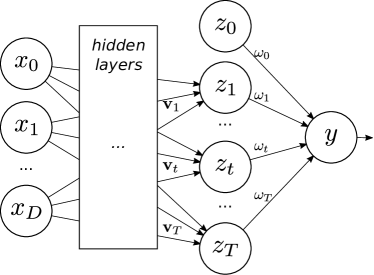
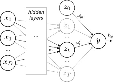
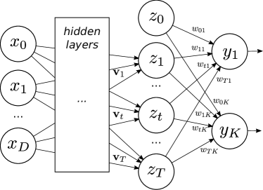
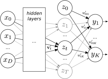
Figure 1: Illustration of binary and multi-class neural networks and their parameters (left diagrams) and neural networks with one unit highlighted in black that represents the $t^{th}$ model trained in gradient boosted neural network (right diagrams).

2.4 Neural network as an additive expansion

A multi-layered neural network can be seen as an additive expansion of its last hidden layer. The output of the last hidden layer for a fully connected neural network for binary tasks is (using the parametrization shown in Fig 1 top left)

$$p(y=1|\mathbf{x})=\sigma\left(\sum_{t=0}^{T}\omega_{t}z_{t}\right)$$ (17)

and for multi-class (bottom left in Fig 1)

$$p(y=k|\mathbf{x})=\sigma\left(\sum_{t=0}^{T}\omega_{tk}z_{t}\right)$$ (18)

with $z_{t}$ being the outputs of the last hidden layer, $\omega_{t}$ and $\omega_{tk}$ the weights of the last layer and $\sigma$ the activation function (for classification). For regression, no activation function is used. It is not straightforward to adapt this process to train deeper layers as we take advantage of the additive nature of the final output of the network. In the standard NN training procedure all parameters of the model (i.e. $\mathbf{v}_{t}$ and $\omega_{k}$ or $\omega_{tk}$ as shown in Figure 1 left diagrams) are fitted jointly with back-propagation. In the proposed method, instead of learning the weights jointly, the parameters are trained sequentially using gradient boosting. To do so, after computing $F_{0}$, a fully connected regression neural network with a single (or few) neuron(s) in the last hidden layer is trained using standard back-propagation. This neural network is trained on the residuals given by the previous iteration as given by Eq. 7 for binary classification and Eq. 12 for multi-class classification tasks. Note that, this network trained on the residuals could have a single or several units in the hidden layer. In the remainder of this section we will assume that at each step of the boosting procedure a network with one single unit in the hidden layer is used. Generalizing this to larger networks is trivial. Figure 1 (right diagrams) shows, highlighted in black, the regression neural network with a single neuron in the hidden layer that is trained in iteration $t$ and that corresponds to model $h_{t}$. After model $t$ has been trained, the value of $\rho_{t}$ is computed using Eq. 8 for binary problems and $\rho_{k,t}$ (Eq. 15) for multi-class classification. Once all $T$ models have been trained, a neural network, as shown in Figure 1 (left diagrams), with $T$ units in the last hidden layer is obtained by assigning all the weights necessary to compute the $z_{t}$ variables (i.e. ${\mathbf{v}_{t}}^{\prime}$ in Figure 1 right) to the corresponding weights in the final NN (i.e. ${\mathbf{v}_{t}}$ in Figure 1 left) for binary and multi-class tasks

$$\mathbf{v}_{t}=\mathbf{v}_{t}^{\prime}\;\;\;\;t=1,\dots,T$$ (19)

and the weights $\omega_{t}$ of the output layer for binary classification are assigned to

$$\omega_{0} =F_{0}+\sum_{t=1}^{T}2\rho_{t}{\omega^{\prime}}_{t0}$$ (20)

$$\omega_{t} =2\rho_{t}\omega^{\prime}_{t}\;\;\;\;t=1,\dots,T$$ (21)

where the ${\omega^{\prime}}_{t}$ and ${\omega^{\prime}}_{t0}$ are the weights from the hidden neuron to the output and the bias term respectively for the $h_{t}$ model (as shown in Figure 1 right-top diagram). For multi-class with $K$ classes final the assignment is

$$\omega_{0k} =\sum_{t=1}^{T}\rho_{k,t}{\omega^{\prime}}_{t0k}$$ (22)

$$\omega_{tk} =\rho_{k,t}\omega^{\prime}_{tk}\;\;\;\;t=1,\dots,T\;\;k=1,\dots,K$$ (23)

where the ${\omega^{\prime}}_{tk}$ and ${\omega^{\prime}}_{t0k}$ are the output weights for the $h_{t}$ multi-class model (Figure 1 right-bottom diagram).

Finally, to recover the probability of $y=k|\mathbf{x}$ in the output of the NN as given by Eq. 9 and Eq. 16, the activation function should be a sigmoid (i.e. $\sigma(x)=1/(1+\exp(-x)$) for binary classification with the logistic loss (Eq. 6), and the soft-max activation function (i.e. $\sigma(\mathbf{x})=exp(x_{k})/\sum_{k}exp(x_{k})$) for multi-class tasks when using the cross-entropy loss (Eq. 10). This training procedure can be easily modified to larger increments of neurons, so that instead of a single neuron per step (a linear model), a more flexible model, comprising more units ($J$), can be trained at each iteration. The outline of the proposed method is shown in Algorithm 1.

The proposed training procedure can be further tuned by applying subsampling and/or shrinking, as generally used in gradient boosting [20, 19, 9]. In shrinking, the additive expansion process is regularized by multiplying each term $\rho_{t}h_{t}$ by a constant learning rate, $\nu\in(0,1]$, to prevent overfitting when multiple models are combined [19]. Subsampling consists of training each model on a random subsample without replacement from the original training data. Subsampling has shown to improve the performance of gradient boosting [20].

The overall computational time complexity to train the proposed algorithm is the same as that of a standard NN with the same number of hidden neurons and training epochs. Note that, at each step of the proposed algorithm, one NN with one (or few) neurons in the hidden layer is trained. Hence, at the end of the process, the same number of weights updates are performed. Note, however, that the proposed method is sequential and cannot be easily parallelized. Once the model is trained, the computational complexity for classifying new instances is equivalent to that of a standard NN as the generated model is a standard neural network.

Algorithm 1 Training Neural network as an additive expansion

Input

1:Input data $D=\{\mathbf{x}_{i},y_{i}\}_{1}^{N}$

2:Number of neurons $T$

3:Loss function

Training the model

1:Initialize ${\hat{F}}_{0}$

2:for $t=1$ to $T$ do

3:     Compute the pseudo-residual with Eqs. 7 12 ($r_{ti}$ for binary and $r_{tik}$ for multi-class classification)

4:     Fit a new regressor network model on the residuals.

5:     Compute the gradient descent step through the Newton-Raphson step ($\rho_{t}$ for binary, Eq. 8 and $\rho_{kt}$ for multi-class classification, Eq. 15)

6:     Update the model using Eq.1

7:end for

8:Create the final network by assigning the weights with Eqs. 19 21 23

2.5 Illustrative example

To illustrate the workings of this algorithm, we show its performance in a toy classification problem. The toy problem task consists in a 2D version of the ringnorm problem [5]: where both classes are 2D Gaussian distribution, one with $(0,0)$ mean and covariance four times the identity matrix, and the second class with mean value at $(2/\sqrt{2},2/\sqrt{2})$ and the identity matrix as covariance.

The proposed gradient boosted neural network (GBNN) with $T=100$ and one hidden layer is trained on $200$ randomly generated instances of this problem. In addition, $100$ independent neural nets with hidden units in the range $[1,100]$ are also trained using the same training set. In Figure 2, the boundaries for the different stages of the process are shown graphically. In detail, the first and second rows show the results for GBNN and NN, respectively. Each column shows the results for $T=1$, $T=2$, $T=3$, $T=4$ and $T=100$ neurons in the hidden layer respectively. Note that the plots for GBNN are sequential; That is, the first column shows the first trained model, the second column, the first two models combined, and so on. For the NN, each column corresponds to a different NN with a different number of neurons in the hidden layer. For each column, the architecture of the networks and the number of weights (but not their values) are the same. The color of the plots represent the probability $p(y=1\mid\mathbf{x})$ given by the models (Eq. 9) using the viridis colormap. In addition, all plots show the training points.

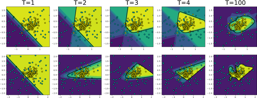
Figure 2: Classification boundaries for gradient boosted neural network (top row) and for a standard neural network (bottom row). Each column shows the results for a combination of a different number of models (hidden units). Top plots are the sequential results of a single GBNN model, whether bottom plots are independent neural networks models

As we can see both GBNN and NN start, as expected, with very similar models (column $T=1$). As the number of models (neurons for NN) increases, GBNN builds up the boundary from previous models. On the other hand, the standard neural network, as it creates a new model for each size, is able to adjust faster to the data. However, as the number of neurons increases, NN tends to overfit in this problem (as shown in the bottom right-most plot). On the contrary, GBNN tends to focus on the unsolved parts of the problem: the decision boundary becomes defined only asymptotically, as the number of models (neurons) becomes large.

3 Experimental results

In this section, an analysis of the efficiency of the proposed neural network training method based on gradient boosting is tested on twelve binary classification tasks, eight multi-class problems, seven regression datasets from the UCI repository [29], and two datasets related to image processing [14, 27]. These datasets, shown in Table 1, have different number of instances and attributes and come from different fields of application. The Energy dataset has two different target columns (cooling and heating), so the different algorithms were executed for both objectives separately. We modified some of the datasets. For Diabetes duplicated instances and instances with missing values were removed. In addition, categorical values were substituted by dummy variables in: German Credit Data, Hepatitis, Indian Liver Patient, MAGIC and Tic-tac-toe. Finally, CIFAR-10 and MNIST were normalized by dividing the attributes by 255.

Dataset	Area	Instances	Attribs.
Binary classification
Australian Credit Approval	Financial	690	14
German Credit Data	Financial	1,000	20
Banknote	Computer	1,372	5
Spambase	Computer	4,601	57
Tic-tac-toe	Game	958	9
Breast cancer	Life	569	32
Diabetes	Life	381	9
Hepatitis	Life	155	19
Indian Liver Patient	Life	583	10
MAGIC Gamma Telescope	Physical	19,020	11
Ionosphere	Physical	351	34
Sonar	Physical	208	60
Multi-class classification
Digits	Computer	1,797	64
Poker Hand	Game	1,025,010	10
Iris	Life	150	4
Covertype	Life	581,012	54
Vehicle	Transportation	946	18
Vowel	Education	990	11
Waveform	Physical	5,000	21
Wine	Physical	178	13
Regression
Concrete	Physical	1,030	9
Energy	Computer	768	8
Power	Computer	9,568	4
Boston Housing	Business	506	14
Wine quality-red	Business	1,599	12
Wine quality-white	Business	4,898	12
image processing
MNIST	handwritten digits	60,000	28x28
CIFAR-10	labeled images	60,000	32x32

Table 1: The details of datasets, which used in experimental analysis

Two batches of experiments were carried out: experiments on tabular data and experiments on image and large datasets. In the first batch, the proposed method is compared with respect to standard neural networks using different solvers and with respect to dense deep neural networks. In the second batch, a transfer learning approach was followed, training the last layer of deep models with the proposed method and fully connected NN. The first experiment is carried out in all the classification and regression tasks shown in Table 1, except for Covertype, Poker Hand, MNIST and CIFAR-10. For these large datasets, the comparison of the proposed method was carried out with respect to deep dense or convolutional neural networks, depending on the type of problem. For the first batch of experiments, the scikit-learn package [34] was used. For the second batch, we adopted Keras library [10]. The implementation of the proposed method (GBNN) is done in python following the standards of scikit-learn. The implementation of the algorithm is available on https://github.com/GAA-UAM/GBNN/.

3.1 Experiments with tabular data

For the first set of experiments on tabular regression and classification, single hidden layer networks were trained using three different standard solvers (Adam, L-BFGS and SGD), and using the proposed gradient boosting approach. Also, we considered a three-layer deep dense neural network trained with the Adam solver. Furthermore, AdaBoost [17] using small neural networks as the base models was also included in the comparison (AdaBoost–NN). Note that, this approach is different to the proposed GBNN. First, for classification tasks, the base models in Adaboost are classifiers that are combined by weighted majority voting. Hence, the final model is a collection of small base classifiers and not a single neural network as in GBNN. Second, Adaboost is based on modifying the instance weights during training so that difficult instances tend to get higher weights. This poses a difficulty in the training of the neural networks as they do not handle weighted instances. In order to run Adaboost with neural networks we included a weighted resampling step prior the training of each individual network. The sklearn library does not include this functionality in Adaboost. The comparison for classification and regression problems was carried out using 5$\times$10-fold cross-validation in order to have stable results. For the Waveform dataset we also considered 10 random train-test partitions using 300 instances for training the models and the rest for test as experiments with this dataset generally consider this experimental setup [5]. All datasets were standardized in train so that all attributes have zero mean and one variance. The optimum hyper-parameter setting for each method was estimated using within-train 10-fold cross-validation. For the standard neural network with the standard solvers, the grid with the number of units in the hidden layer was set to [1, 3, 5, 7, 11, 12, 17, 22, 27, 32, 37, 42, 47, 52, 60, 70, 80, 90, 100, 150, 200]. In addition, for the SGD solver, the learning policies $[Adaptive,Constant]$ were also considered in its grid search. The rest of the hyper-parameters were set to their default values. Regarding the three-layer deep network, 100 neurons per layer were used and all the other hyper-parameters were left to their default values. For GBNN, a sequentially trained neural network with 200 hidden units is built in steps of $J$ units per iteration. For this model, the hyper-parameter grid search was carried out using the following values for binary classification: $[0.1,0.25,0.5,1.0]$ for the learning rate, $[0.5,0.75,1.0]$ for subsample rate and $J\in[1,2,3]$. For the multi-class and regression problems the hyper-parameter grid was extended a bit because in some datasets the values at the extremes were always selected. Hence, the grid for multi-class and regression problems is set to: $[0.025,0.05,0.1,0.5,1]$ for the learning rate, $[0.25,0.5,0.75,1.0]$ for subsample rate and $J\in[1,2,3,4]$. Moreover, for the proposed procedure, the sub-networks are trained using the L-BFGS solver for all datasets. This decision was made after some preliminary experiments that showed that L-BFGS provided good results in general for the small networks we are training at each iteration. Regarding AdaBoost-NN, a classification/regression one hidden layer perceptron is set as base estimator. The number of estimators to include in the ensemble and number of hidden neurons were set respectively to the following pairs: (200,1), (100,2) and (67,3). For multi-class problems the pair (50, 4) was also considered. This is done in order to produce a model with a combined total number of 200 hidden neurons as for previous networks. Subsequently, the best sets of hyper-parameters obtained in the grid search for each method were used to train the whole training set, one standard neural network for each solver, dense deep neural networks, AdaBoost–NN, and the proposed gradient boosted neural network. Finally, the average generalization performance of the models was estimated in the left-out test set.

For all analyzed datasets, the average generalization performance and standard deviations are shown in Table 2 for the proposed method (column GBNN), the three-layer deep neural network (column Deep-NN), standard neural networks trained with Adam (NN–Adam), L-BFGS (NN–L-BFGS), SGD (NN–SGD), and AdaBoost–NN. For classification problems the generalization performance is given as average accuracy and, for regression, as average root mean square error. The Table 2 is structured in three blocks depending on the problem type: binary classification tasks, multi-class classification, and regression. The best result for each method is highlighted with a light yellow background. An overall comparison of these results is shown graphically in Figure 3 using the methodology described in [12]. These plots show the average rank for the studied methods across the analyzed datasets where a higher rank (i.e. lower values) indicates better results. The figure shows the Demsǎr plots for the classifications tasks only (top left plot), for regression only (top right plot), and for all analyzed tasks (bottom plot). The statistical differences between methods are determined using a Nemenyi test. In the plot, the difference in the average rank of the two methods is statistically significant if the methods are not connected with a horizontal solid line. The critical distance (CD) in average rank over which the performance of two methods is considered significant is shown in the plot for reference (CD = 1.72, 2.84, and 1.47 for 19 classification, 7 regression and all datasets respectively, considering 6 methods and p-value $<0.05$).

Dataset	GBNN	Deep-NN	NN–Adam	NN–L-BFGS	NN–SGD	AdaBoost–NN
Binary classification
Australian Credit Approval	85.91%$\pm$4.81	82.81%$\pm$4.26	85.88%$\pm$4.43	86.20%$\pm$4.32	86.35%$\pm$4.28	84.58 %$\pm$3.32
Banknote	99.99%$\pm$0.04	100.00%$\pm$0.00	99.99%$\pm$0.04	99.81%$\pm$0.42	97.32%$\pm$1.15	100.00%$\pm$0.00
Breast cancer	96.87%$\pm$1.93	97.40%$\pm$2.06	97.36%$\pm$1.97	96.83%$\pm$1.55	96.55%$\pm$1.69	96.45%$\pm$4.72
Diabetes	76.12%$\pm$3.93	71.30%$\pm$4.59	76.35%$\pm$4.05	76.67%$\pm$ 4.15	76.96%$\pm$ 4.21	74.81%$\pm$ 3.25
German Credit Data	74.16%$\pm$3.64	69.84%$\pm$4.53	73.74%$\pm$3.99	72.34%$\pm$ 3.41	73.28%$\pm$ 3.87	72.44%$\pm$ 4.42
Hepatitis	82.81%$\pm$ 10.60	84.10%$\pm$ 10.83	85.10%$\pm$ 10.86	82.11%$\pm$ 9.21	85.09%$\pm$ 10.65	85.54%$\pm$ 7.82
Indian Liver Patient	72.51%$\pm$5.30	70.88%$\pm$ 5.20	70.69%$\pm$ 5.81	69.44%$\pm$ 5.88	71.10%$\pm$ 5.52	69.26%$\pm$4.84
Ionosphere	90.94%$\pm$ 4.86	93.28%$\pm$3.69	91.34%$\pm$3.92	90.43%$\pm$4.58	87.90%$\pm$5.96	92.25%$\pm$3.52
MAGIC Gamma Telescope	87.52%$\pm$0.67	85.62%$\pm$0.85	87.65%$\pm$0.57	87.58%$\pm$ 0.62	86.28%$\pm$ 1.48	87.19%$\pm$0.75
Sonar	78.84%$\pm$7.30	86.22%$\pm$7.57	85.56%$\pm$6.48	85.29%$\pm$ 5.07	77.67%$\pm$ 7.67	85.91%$\pm$8.26
Spambase	94.44%$\pm$1.00	94.08%$\pm$1.22	94.61%$\pm$1.01	93.43%$\pm$ 1.27	93.42%$\pm$ 1.27	74.20%$\pm$13.16
Tic-tac-toe	98.70%$\pm$1.17	95.78%$\pm$1.80	90.44%$\pm$3.19	93.53%$\pm$ 2.56	70.94%$\pm$ 4.30	86.75%$\pm$3.69
Multi-class classification
Digits	97.18%$\pm$1.21	97.55%$\pm$1.06	98.04%$\pm$1.11	97.17%$\pm$1.10	96.44%$\pm$1.09	95.66%$\pm$1.18
Iris	95.73%$\pm$ 6.02	94.40%$\pm$6.58	95.33%$\pm$5.58	94.93%$\pm$6.57	85.07%$\pm$ 8.71	94.72%$\pm$2.16
Vehicle	84.61%$\pm$3.92	83.41%$\pm$3.82	83.43%$\pm$3.52	82.96%$\pm$4.21	72.99%$\pm$4.51	72.13%$\pm$4.15
Vowel	89.88%$\pm$2.57	96.71%$\pm$1.96	94.28%$\pm$2.36	93.13%$\pm$3.09	53.04%$\pm$4.34	51.45%$\pm$3.37
Waveform	87.00%$\pm$ 1.16	82.60%$\pm$ 1.62	86.65%$\pm$1.40	86.46%$\pm$ 1.22	86.68%$\pm$ 1.37	84.99%$\pm$1.46
Waveform-300	82.94%$\pm$ 0.17	82.07%$\pm$ 0.63	83.69%$\pm$0.70	79.51%$\pm$ 0.02	83.92%$\pm$ 0.77	84.55%$\pm$0.40
Wine	98.88%$\pm$ 2.35	97.87%$\pm$ 3.35	97.77%$\pm$ 3.22	97.65%$\pm$3.50	95.72%$\pm$4.91	97.32%$\pm$3.48
Regression
Boston Housing	3.03%$\pm$0.74	3.18%$\pm$0.79	4.12%$\pm$0.77	3.50%$\pm$0.98	3.40%$\pm$ 0.87	14.43%$\pm$1.49
Concrete	4.80%$\pm$0.59	5.20%$\pm$0.56	9,61%$\pm$0.58	4.73%$\pm$0.59	6.04%$\pm$ 0.47	26.78%$\pm$1.10
Energy-Cooling	0.95%$\pm$0.16	2.16%$\pm$0.31	3.45%$\pm$0.46	1.14%$\pm$0.17	3.12%$\pm$0.41	15.91%$\pm$1.69
Energy-Heating	0.43%$\pm$0.08	1.40%$\pm$0.27	2.96%$\pm$0.38	0.49%$\pm$0.06	2.75%$\pm$0.33	12.95%$\pm$1.29
Power	3.84%$\pm$0.18	4.40%$\pm$0.39	4.25%$\pm$0.16	4.11%$\pm$ 0.17	4.14%$\pm$0.15	123.37%$\pm$9.70
Wine quality-red	0.60%$\pm$0.04	0.68%$\pm$0.06	0.64%$\pm$0.05	0.64%$\pm$0.73	0.65%$\pm$0.04	0.83%$\pm$0.06
Wine quality-white	0.67%$\pm$0.03	0.72%$\pm$0.04	0.68%$\pm$0.03	0.70%$\pm$0.03	0.70%$\pm$0.03	0.74%$\pm$0.02

Table 2: Average generalization performance and standard deviation for gradient boosted neural network (GBNN), Deep neural network, neural networks trained with solvers Adam, L-BFGS, SGD and AdaBoost. Using accuracy for the classification tasks and root mean square error (RMSE) for regression problems as the performance measurement. The best results for each dataset are highlighted with a light yellow background.

From Table 2 and Figure 3, it can be observed that, for the studied datasets, the best overall performing method is GBNN. This method reached the best results in 13 out of 26 tasks. The deep-NN model performed best in five datasets. The neural network method with Adam as its solver captured the best results in three datasets. SGD and L-BFGS solvers obtained the best outcome in two and one datasets, respectively. And finally, the AdaBoost–NN got the best performance in three datasets. In classification, the differences in average accuracy among the different methods are generally favorable to GBNN, NN–Adam and Deep–NN, although the differences between these methods are small in many datasets. For instance, in Magic, the accuracy of GBNN is only 0.13 percent points worse than NN–Adam. However, small differences are not always the case. One of the most notable differences between GBNN and second top ranked method is in Tic-tac-toe where Deep–NN is 2.92% worse than the result obtained by GBNN and NN-Adam is more than 8 points worse. In contrast, the most favorable outcome for Deep–NN is obtained in Vowel and Sonar, where its accuracy is 6.83% and 7.38% better than that of GBNN, respectively. The results in classification for NN–L–BFGS, NN–SGD and AdaBoost–NN are generally worse than those of the other three methods.

In regression, the results are more clearly in favor of GBNN. The proposed method obtains the best performance in all tested datasets except for one dataset, Concrete, in which GBNN get the second best result. The performance of NN–Adam in regression is suboptimal getting the worst performances in general. Solver L-BFGS perform more closely to the performance of GBNN.

These results can also be observed from Figure 3. The performance of NN–L-BFGS, NN–SGD and AdaBoost–NN in the classification tasks is worse than that of NN–Adam, GBNN and Deep–NN (subplot a). NN-Adam and GBNN take the highest rank in the statistical test. For regression (subplot b), the best-performing method is GBNN. The performance of GBNN is significantly better than that of NN–Adam, NN–SGD and AdaBoost–NN. The overall results (subplot c) show that GBNN has the best rank followed by NN–Adam and Deep–NN. Overall, the performance of GBNN is statistically better than the performance of NN–SGD and AdaBoost-NN.

(a) Classification

(b) Regression

(c) All of the datasets

Figure 3: Average ranks (higher rank is better) for GBNN, Deep-NN, NN–Adam, NN–L-BFGS, NN–sgd and AdaBoost–NN for 26 datasets. a) The Demsǎr plot for binary and multiclass datasets. b) The Demsǎr plot for regression datasets. c) The Demsǎr plot considering all of the datasets.

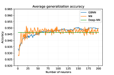
(a) Spambase

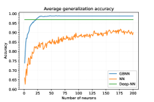
(b) Tic-tac-toe

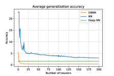
(c) Energy-Heating

Figure 4: Average generalization accuracy for GBNN (blue curve), NN (orange curve), and Deep-NN (green curve) with respect to the number of hidden units

To analyze the evolution of the networks generated by the proposed method as more hidden units are included, another experiment was carried out to build a GBNN with 200 hidden units, and neural networks trained using the Adam solver with 1 to 200 neurons in the hidden layer. In addition, the final accuracy of a three-layer deep neural network with 100 neurons in each layer is also computed for reference. For this experiment, 10-fold cross-validation was used. The average evolution is shown in Figure 4 for Spambase (left plot), Tic-tac-toe (middle plot) and Energy-Heating (right plot). Due to computational limitations in this case, the hyper-parameters were not tuned for each partition. Instead, they were set to the values more often selected in the previous experiment for each dataset. Specifically, they were set to $J=3$, learning rate to 0.5 and subsampling to 1 for Tic-tac-toe, to $J=1$, learning rate to 0.5 and subsampling to 0.75 for Spambase and to $J=4$, learning rate to 0.5 and subsampling to 1 for Energy-Heating for all partitions. Note that for each sequence of GBNN, only one model is trained. For NN, 200 independent models with 1 to 200 neurons need to be trained in order to obtain the sequence.

From Fig 4, it can be observed that the average test accuracy of GBNN improves as more units are considered. More importantly, we can observe that GBNN tends to stabilize with the number of units. Hence, if the latter units are removed, the performance in the model accuracy is not damaged to a great extent. For instance, in Spambase, if the number of units is reduced from $T=200$ to $T=100$ the model accuracy only drops from $94.78\%$ to $\approx 94.63\%$. In Tic-tac-toe the same size reduction does not reduce the accuracy of the model. This observation also applies for the Energy-Heating regression task. This property can be useful, as one can adopt a single model to different computational requirements on the fly. The performance of NN could be higher than that of GBNN at some stages (as shown for Spambase), however, the number of hidden neurons to use have to be decided during train. In addition, the performace of two neural networks with $T$ and $T+1$ trained on the same data present a higher variance than a single GBNN model using $T$ and $T+1$. Hence, the performance of the sequence of NN is not as monotonic as the sequence of GBNN.

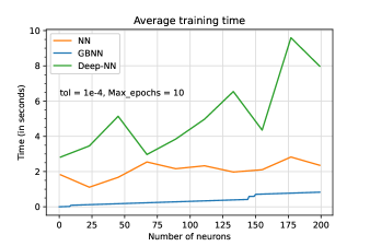
(a) Power

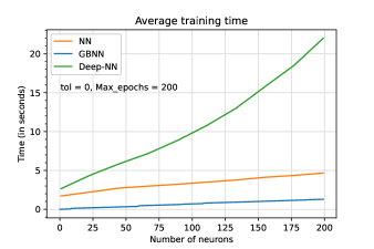
(b) Power

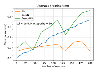
(c) Indian Liver Patient

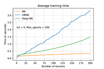
(d) Indian Liver Patient

Figure 5: Average training time (in seconds) for gradient boosted neural network (Blue curve), standard neural network (orange), and deep neural network (green), for waveform (top row) and Indian liver patient (bottom row). In the left column, the default early stopping procedure was set to train the networks of all models (tolerance is set to $1e-4$ and iterations with no change to ten). In the right column, all networks are force to train during 200 epochs (tolerance is set to 0 and max iterations without change to 200)

In order to compare the computational performance of the tested methods, the training time for GBNN, Deep-NN, NN–Adam, NN-L-BFGS and NN-SGD are shown in Table 3. For this experiment, we applied 10-fold cross-validation and computed the average fit time of the final model that used the set hyper-parameters most frequently selected in the cross-validation. The size for GBNN and the different networks was set to 200. Deep-NN was built, as before with three layers of 100 neurons each. GBNN uses the solver L-BFGS. This experiment is done on CPU using AMD Ryzen 7 5800H 3.20 GHz processor. As Table 3 illustrates, the most computationally efficient method is NN–SGD followed by NN–L-BFGS. In general, the differences are rather contained among most methods and datasets. Some exceptions include the Deep-NN with respect to the other methods, which could be up to x20 slower (e.g. Power or Energy-Heating). The variance in the average times among the different methods for each dataset is also due to the fact that the default hyper-parameters for all methods include an early-stopping strategy in which the training stops if the loss does not drop at least $0.0001$ in ten training iterations. In order to visualize this effect, in Figure 5 we show the average training time with respect of the number of neurons in the hidden layers for GBNN, Deep-NN and NN-Adam for two datasets (one favorable to GBNN and one favorable to NN). The left plot shows the results considering early stopping and the right plot forces the networks to train for 200 epochs. Note that the results of GBNN are monotonic since a single model is used to obtain the training time sequence. For Deep-NN and NN-Adam, a different model is trained every 20 hidden neurons, which explains the peaks in the curves especially when early stopping is active (left plots). When the models are forced to train for 200 epochs, the evolution of the shallow models show a clear linear complexity with respect to the number of hidden units. The deep model shows a quadratic complexity in accordance with the growth of the number of weights. In addition, the training time performance of GBNN is also affected by the model setting. This can account for the favorable and unfavorable results for GBNN shown in Figure 5. In particular, in some exploratory experiments we carried out using different learning rates illustrated that the higher the learning rate, the slower the training time specially for classification.

Dataset	GBNN	Deep-NN	NN–Adam	NN–L-BFGS	NN–SGD
Binary classification
Australian Credit Approval	1.105	0.236	0.093	0.614	0.359
Banknote	0.454	0.391	0.515	0.065	1.055
Breast cancer	0.165	0.295	0.305	0.510	0.054
Diabetes	0.882	0.253	0.698	0.619	0.221
German Credit Data	0.129	0.187	0.208	0.130	0.524
Hepatitis	0.316	0.060	0.023	0.247	0.046
Indian Liver Patient	0.557	0.220	0.288	0.073	0.400
Ionosphere	0.791	0.618	0.431	0.085	0.400
MAGIC Gamma Telescope	5.273	37.267	6.177	12.931	5.038
Spambase	2.240	2.461	0.903	5.057	0.639
Sonar	0.568	0.581	0.327	0.166	0.307
Tic-tac-toe	0.732	1.215	1.011	0.413	0.956
Multi-class classification
Digits	0.976	1.095	1.016	0.463	2.369
Iris	1.288	0.321	0.108	0.142	0.102
Vehicle	0.256	0.519	0.269	0.549	0.391
Vowel	1.088	1.992	1.419	0.578	1.085
Waveform	3.896	8.676	5.452	3.644	5.146
Wine	0.116	0.348	0.022	0.071	0.041
Regression
Boston Housing	0.636	1.026	0.468	0.344	0.030
Concrete	0.453	0.650	0.672	0.673	0.045
Energy-Cooling	0.077	0.768	0.632	0.573	0.037
Energy-Heating	0.083	1.023	0.643	0.488	0.037
Power	0.198	4.093	1.709	1.330	0.321
Wine quality-red	1.192	1.748	0.865	0.995	0.450
Wine quality-white	1.148	1.953	2.647	3.150	0.220

Table 3: Total training time in seconds for gradient boosted neural network (GBNN), deep neural network, and neural networks with Adam solver

3.2 Experiment with large datasets and deep models

For the second batch of experiment, three-layer deep dense network and CNNs were used. In order to compare the deep models with the proposed method, we followed a transfer learning approach. For this, once the deep models are trained, the last dense layer and the output layer of the CNN and Deep-NN are removed. Then, the weights of the first layers are frozen. Finally, a GBNN model is trained linked to the frozen layers using the same training instances. We term this model as Deep-GBNN. For Covertype and Poker Hand, a three-layer deep dense neural network with 100 hidden networks per layer were trained for 200 epochs. The activation functions are ReLu for the internal layers and Sigmoid for the output layer. The solver SGD was applied. For CIFAR-10 and MNIST, a CNN was trained for 200 epochs on the training set. The CNN includes the following layers: two convolutions(32), max-pooling (2x2), dropout(0.2), two convolutions(64), max-pooling (2x2), dropout(0.3), two convolutions(128), max-pooling (2x2), dropout(0.4), two dense(128), and one output dense layer for ten classes. The activation functions are ReLu for the internal layers and SoftMax for the output layer. For these datasets, a single partition train/test was carried out. The dataset is divided into a training and a test set as defined by the dataset: 50000 train and 10000 test for CIFAR-10; 60000 train and 10000 test for MNIST and 25010/1000000 for Poker. For Covertype, a random stratified partition of 70%-30% was done. The optimum hyper-parameters configuration was measured using within-train 5-fold cross-validation, except for Covertype where a 2-fold cross-validation was used. For Deep-GBNN, the values for the grid search were in the following ranges: $[0.1,1]$ for the learning rate, $[0.25,1]$ for subsample and $[1,15]$ for the step size. Also, the solver for the GBNN method was set to Adam, due to better performance in dealing with high-dimensional datasets. In addition, we run the final experiment using pre-trained networks. For that, we used the InceptionV3 [40] and VGG16 [39] models pre-trained on the imagenet dataset [13]. These models were loaded and subsequently fine-tuned on the CIFAR-10 dataset using the default train partition composed of $50,000$ instances. They are validated on the remaining $10,000$ test instances. Finally, we froze the weights of VGG16 and InceptionV3 and replaced their last dense layer with a optimized GBNN and NN with 500 units, in which the optimization had done using grid search using train. Finally, the accuracy of NN and GBNN is estimated on the test set.

The Table 4 presents the achieved accuracy for four datasets in the test set (first two columns) and the estimation of the generalization accuracy obtained in the in-train cross-validation (last two columns). The best in-train and test results are highlighted with a yellow background. The results show uneven performance for the different dataset. The proposed method manages to improve the performance of the deep models in MNIST, Cover type and Poker hand by 0.06, 1.76 and 0.12 percentage points respectively. In CIFAR-10, performance drops by 0.03%. Even if the differences are in general marginal, an interesting aspect is that the in-train performance can be used to select the best model on each dataset except in MNIST. Although the differences between method in this dataset both in-train and in test are negligible. Finally, the performances of the GBNN and NN models trained on the output of InceptionV3 and VGG16 for CIFAR-10, and the fine-tuned transfer learning models as well are shown in Table 5. The application of GBNN on top of the pre-trained and fine-tuned models, gained 0.08 and 0.07 percent points in accuracy with respect to InceptionV3 and VGG16 respectively. The results of NN are 0.08 percentage points worse and 0.08 better than the deep fined-tuned models. The accuracy improvements of using GBNN on top of the deep models is small but as it is the additional computational training cost. The classification computational cost remains the same.

	Test estimation		In-train estimation
Dataset	Deep-GBNN	Deep-CNN	Deep-GBNN	Deep-CNN
CIFAR-10	84.09	84.12	82.77	83.04
MNIST	99.52	99.46	99.35	99.42
	Deep-GBNN	Deep-NN	Deep-GBNN	Deep-NN
CoverType	90.00	88.24	87.53	83.45
Poker Hand	99.45	99.33	98.57	97.72

Table 4: Average generalization performance (first two columns) and in-train performance (second two columns) for deep gradient boosted neural networks (Deep-GBNN) and Deep Convolutional Neural Networks (Deep-CNN).

	Fine-tuned	GBNN		NN
Pre-trained model	Test	Test	In-train	Test	In-train
InceptionV3	93.12	93.20	99.99	93.04	99.98
VGG16	92.92	92.99	99.98	93.00	99.98

Table 5: The generalization performance of the fine-tuned transfer learning models for each model (InceptionV3 and VGG16). And generalization and in-train performance of a one-layer GBNN and NN-trained models on the output of pre-trained models on the CIFAR-10.

4 Conclusions

In this paper, we present a novel iterative method to train a neural network based on gradient boosting. The proposed algorithm builds at each step a regression neural network with one or few ($J$) hidden unit(s) fitted to the data residuals. The weights of the network are then updated with a Newton-Raphson step to minimize a given loss function. Then, the data residuals are updated to train the model of the next iteration. The resulting $T$ regressors constitute a single neural network with $T\times J$ hidden units. In addition, the formulation derived for this works opens the possibility to create gradient boosting ensembles composed of base models different from decision trees, as done in previous implementations of gradient boosting.

In the analyzed problems, the proposed method achieves a generalization accuracy that converges with the number of combined regressors (or hidden units). This quality of the proposed method allows us to use the combined model fully or partially by deactivating the units in order inverse to their creation, depending on classification speed requirements. This can be done on the fly during the test. In addition, we showed that the training complexity is equivalent to that of training a network with a standard solver.

The proposed method tested on a variety of classification, regression and image processing tasks. The results show a performance favorable to the proposed method in general. The proposed approach showed the best overall average rank in the tested classification and regression problems with statistically significant differences with respect to SGD and L-BFGS approaches. In addition, for deep models a transfer learning approach was followed and the results were favorable to the proposed method in some of the tasks although the differences were small. Notwithstanding, the proposed iterative training procedure opens novel alternatives for training neural networks. This particularly evident for regression tasks where the proposed method achieved the best result in most of the analyzed datasets.

Machine learning is becoming a fundamental piece for the success of more and more applications every day. Some examples of novel applications include bioactive molecule prediction [1], renewable energy prediction [41], classification of galactic sources [31], or agriculture area for mapping soil contamination [24]. It is of capital importance to find algorithms that can efficiently handle complex data. Ensemble methods are very effective at improving the generalization accuracy of multiple simple models [16, 7] or even complex models such as MLPs [38] or DeepCNNs [32].

In recent years, gradient boosting [19, 18], a fairly old technique has gained much attention, specially due to the novel and computationally efficient version of gradient boosting called eXtreme Gradient Boosting or XGBoost [9]. Gradient boosting builds a model as an additive expansion of regressors to gradually minimize a given loss function. When gradient boosting is combined with several stochastic techniques, as bootstrapping or feature sampling from random forest [6], its performance generally improves [20]. In fact, this combination of randomization techniques and optimization has placed XGBoost among the top contenders in Kaggle competitions [9] and provides excellent performance in a variety of applications as in the ones mentioned above. Based on the success of XGBoost, other techniques have been proposed like CatBoost [35] and LightGBM [25], which propose improvements in training speed and generalization performance. More details about these methods can be seen in the comparative analysis of Bentéjac et al. [3]. Other type of widespread boosting algorithm is AdaBoost [17], initially developed for binary classification and then for multi-class classification (AdaBoost-SAMME) [21] and regression [15].

On the other hand, convolutional deep architectures have shown outstanding performances especially with structured data such as images, speech, etc. [28, 37]. However, in the context of tabular data, ensembles of classifiers or simple MLPs are generally more effective than convolutional deep neural networks [43]. The objective of this study is to combine the stage-wise optimization of gradient boosting into the training procedure of the last layers of a neural network. The result of the proposed algorithm is an alternative for training a single neural network (not an ensemble of networks).

Several related studies propose hybrid algorithms that, for instance, transform a decision forest into a single neural network [42, 4] or that use a deep architecture to train a tree forest [26]. In [42], it is shown that a pre-trained tree forest can be cast into a two-layer neural network with the same predictive outputs. First, each tree is converted into a neural network. To do so, each split in the tree is transformed into an individual neuron that is connected to a single input attribute (split attribute) and whose activation threshold is set to the split threshold. In this way, and by a proper combination of the outputs of these neurons (splits) the network mimics the behavior of the decision tree. Finally, all neurons are combined through a second layer, which recovers the forest decision. The weights of this network can be later retrained to obtain further improvements [4]. In [26], a decision forest is trained jointly by means of a deep neural network that learns all splits of all trees of the forest. To guide the network to learn the splits of the trees, a procedure that trains the trees using back-propagation, is proposed. The final output of the algorithm is a decision forest whose performance is remarkable in image classification tasks.

In other related line of work [33, 23], boosting is applied to the construction of Deep Residual Learning models [22]. In [33], a novel ResNet weight estimation model is proposed by generalizing the boosting functional gradient minimization [30] to the feature extraction space of the network. The work presented in [23] also builds layer-by-layer a ResNet boosting over features, however, it is based on a different boosting framework [17]. The model (called BoostResNet) works by learning a linear classifier on the output of each residual network block to build an ensemble of shallow blocks. One important advantage of BoostResNet over standard ResNet is its lower computational complexity although the reported performance is not consistently better with respect to ResNet. In contrast, the current proposal method, based on [19], builds a simple shallow network in-width rather than complex model in-depth and shows very good performance in tabular datasets with respect to standard back-propagation training methods. Furthermore, our proposal can adapt on the fly to the use of a reduced number of hidden neurons.

Another model that resembles the idea proposed in this paper –yet with a different optimization process, final model and objective– was presented in [2]. They propose a convex optimization algorithm for training a neural network that theoreticallly could reach the global optimum although its exact implementation is only feasible for a very low number of input features. In order to reach the global optimum they control the number of hidden neurons of the model by adding one neuron at a time to the network and by including a $L^{1}$ regularization on the top layer. The proposed idea is a stepwise algorithm as all weights of the network are optimized at each iteration. This is done in three optimization steps. First, a new neuron (i.e. linear model) is added and trained on a weighted loss function similarly to Adaboost. This weighted loss can only be solved exactly for a very low number of input features. Then, the output layer, and potentially all input weights, are optimized using the proposed convex formulation. Finally, the output weights are regularized to reduce the complexity of the network. This final step sets to zero some of the output weights to effectively remove the corresponding neurons. The algorithm is tested on one simple 2D problem in order to assess the validity of the global optimum approach.

In this paper, we propose a combination of ensembles and neural networks that is somehow complementary to the work of [26], which is a single neural network that is trained using an ensemble training algorithm. Specifically, we propose to train a neural network iteratively as an additive expansion of simpler models. The algorithm is equivalent to gradient boosting: first, a constant approximation is computed (assigned to the bias term of the neural network), then at each step, a regression neural network with a single (or very few) neuron(s) in the hidden layer is trained to fit the residuals of the previous models. All these models are then combined to form a single neural network with one hidden layer. This training procedure provides an alternative to standard training solvers (such as Adam, L-BFGS or SGD) for training a neural network. Other works related to the optimization and convergence of Adam have been recently proposed [36, 11, 8]. They showed that its convergence can be improved in the context of high dimensional complex image classification tasks. However, their focus is mainly in deep models for image classification tasks.

In addition, the proposed method has an additive neural architecture in which the latest computed neurons contribute less to the final decision. This can be useful in computationally intensive applications as the number of active models (or neurons) can be gauged on the fly to the available computational resources without a significant loss in generalization accuracy. The proposed model is tested on multiple classification and regression problems, as well as in conjunction with deep models posed as transfer learning problems. These experiments show that the proposed method for training the last layers of a neural network is a good alternative to other standard methods.

The paper is organized as follows: Section 2 describes gradient boosting and how to apply it to train a single neural network; In section 3 the results of several experimental analysis are shown; Finally, the conclusions are summarized in the last section.

In this paper, we present a novel iterative method to train a neural network based on gradient boosting. The proposed algorithm builds at each step a regression neural network with one or few ($J$) hidden unit(s) fitted to the data residuals. The weights of the network are then updated with a Newton-Raphson step to minimize a given loss function. Then, the data residuals are updated to train the model of the next iteration. The resulting $T$ regressors constitute a single neural network with $T\times J$ hidden units. In addition, the formulation derived for this works opens the possibility to create gradient boosting ensembles composed of base models different from decision trees, as the all previous implementations.

In the analyzed problems, the proposed method achieves a generalization accuracy that converges with the number of combined regressors (or hidden units). This quality of the proposed method allows us to use the combined model fully or partially by deactivating the units in order inverse to their creation, depending on classification speed requirements. This can be done on the fly during test.

The proposed method has been tested on a variety of classification and regression tasks. The results show a performance favorable to the proposed method in general although the overall differences are not statistically significant with respect to solvers Adam and L-BFGS (they are with respect to SGD). Notwithstanding, the proposed iterative training procedure opens novel alternatives for training neural networks. This is particularly evident for regression tasks where the proposed method achieved the best result in most of the analyzed datasets.

References

- [1] Ismail Babajide Mustapha and Faisal Saeed. Bioactive molecule prediction using extreme gradient boosting. Molecules, 21(8), 2016.
- [2] Yoshua Bengio, Nicolas Roux, Pascal Vincent, Olivier Delalleau, and Patrice Marcotte. Convex neural networks. Advances in neural information processing systems, 18, 2005.
- [3] Candice Bentéjac, Anna Csörgő, and Gonzalo Martínez-Muñoz. A comparative analysis of gradient boosting algorithms. Artificial Intelligence Review, (in press), 2020.
- [4] Gérard Biau, Erwan Scornet, and Johannes Welbl. Neural random forests. Sankhya A, In press, 2018.
- [5] L. Breiman. Bias, variance, and arcing classifiers. Technical Report 460, Statistics Department, University of California, 1996.
- [6] Leo Breiman. Random forests. Machine Learning, 45(1):5–32, 2001.
- [7] Rich Caruana and Alexandru Niculescu-Mizil. An empirical comparison of supervised learning algorithms. In ICML ’06: Proceedings of the 23rd international conference on Machine learning, pages 161–168, New York, NY, USA, 2006. ACM Press.
- [8] Jinghui Chen, Dongruo Zhou, Yiqi Tang, Ziyan Yang, Yuan Cao, and Quanquan Gu. Closing the generalization gap of adaptive gradient methods in training deep neural networks. arXiv preprint arXiv:1806.06763, 2018.
- [9] Tianqi Chen and Carlos Guestrin. Xgboost: A scalable tree boosting system. In Proceedings of the 22Nd ACM SIGKDD International Conference on Knowledge Discovery and Data Mining, KDD ’16, pages 785–794, New York, NY, USA, 2016. ACM.
- [10] Francois Chollet et al. Keras, 2015.
- [11] Aaron Defazio and Samy Jelassi. Adaptivity without compromise: A momentumized, adaptive, dual averaged gradient method for stochastic optimization. arXiv preprint arXiv:2101.11075, 2021.
- [12] Janez Demšar. Statistical comparisons of classifiers over multiple data sets. Journal of Machine Learning Research, 7:1–30, 2006.
- [13] Jia Deng, Wei Dong, Richard Socher, Li-Jia Li, Kai Li, and Li Fei-Fei. Imagenet: A large-scale hierarchical image database. In 2009 IEEE conference on computer vision and pattern recognition, pages 248–255. Ieee, 2009.
- [14] Li Deng. The mnist database of handwritten digit images for machine learning research [best of the web]. IEEE Signal Processing Magazine, 29(6):141–142, 2012.
- [15] Harris Drucker. Improving regressors using boosting techniques. In ICML, volume 97, pages 107–115. Citeseer, 1997.
- [16] Manuel Fernández-Delgado, Eva Cernadas, Senén Barro, and Dinani Amorim. Do we need hundreds of classifiers to solve real world classification problems? Journal of Machine Learning Research, 15:3133–3181, 2014.
- [17] Yoav Freund and Robert E Schapire. A decision-theoretic generalization of on-line learning and an application to boosting. Journal of computer and system sciences, 55(1):119–139, 1997.
- [18] Jerome Friedman, Trevor Hastie, Robert Tibshirani, et al. Additive logistic regression: a statistical view of boosting (with discussion and a rejoinder by the authors). The annals of statistics, 28(2):337–407, 2000.
- [19] Jerome H. Friedman. Greedy function approximation: a Gradient Boosting machine. The Annals of Statistics, 29(5):1189 – 1232, 2001.
- [20] Jerome H. Friedman. Stochastic gradient boosting. Computational Statistics & Data Analysis, 38(4):367 – 378, 2002. Nonlinear Methods and Data Mining.
- [21] Trevor Hastie, Saharon Rosset, Ji Zhu, and Hui Zou. Multi-class adaboost. Statistics and its Interface, 2(3):349–360, 2009.
- [22] Kaiming He, Xiangyu Zhang, Shaoqing Ren, and Jian Sun. Deep residual learning for image recognition. In Proceedings of the IEEE conference on computer vision and pattern recognition, pages 770–778, 2016.
- [23] Furong Huang, Jordan Ash, John Langford, and Robert Schapire. Learning deep resnet blocks sequentially using boosting theory. In International Conference on Machine Learning, pages 2058–2067. PMLR, 2018.
- [24] Xiyue Jia, Yining Cao, David O’Connor, Jin Zhu, Daniel CW Tsang, Bin Zou, and Deyi Hou. Mapping soil pollution by using drone image recognition and machine learning at an arsenic-contaminated agricultural field. Environmental Pollution, 270:116281, 2021.
- [25] Guolin Ke, Qi Meng, Thomas Finley, Taifeng Wang, Wei Chen, Weidong Ma, Qiwei Ye, and Tie-Yan Liu. Lightgbm: A highly efficient gradient boosting decision tree. In Advances in neural information processing systems, pages 3146–3154, 2017.
- [26] Peter Kontschieder, Madalina Fiterau, Antonio Criminisi, and Samuel Rota Bulo. Deep neural decision forests. In The IEEE International Conference on Computer Vision (ICCV), December 2015.
- [27] Alex Krizhevsky, Vinod Nair, and Geoffrey Hinton. Cifar-10 (canadian institute for advanced research). URL http://www. cs. toronto. edu/kriz/cifar. html, 5, 2010.
- [28] Yann LeCun, Yoshua Bengio, and Geoffrey Hinton. Deep learning. Nature, 521:436–444, 2015.
- [29] M. Lichman. UCI machine learning repository, 2013.
- [30] Llew Mason, Jonathan Baxter, Peter Bartlett, and Marcus Frean. Boosting algorithms as gradient descent. Advances in neural information processing systems, 12, 1999.
- [31] N. Mirabal, E. Charles, E. C. Ferrara, P. L. Gonthier, A. K. Harding, M. A. Sánchez-Conde, and D. J. Thompson. 3fgl demographics outside the galactic plane using supervised machine learning: Pulsar and dark matter subhalo interpretations. The Astrophysical Journal, 825(1):69, 2016.
- [32] Mohammad Moghimi, Mohammad Saberian, Jian Yang, Li-Jia Li, Nuno Vasconcelos, and Serge Belongie. Boosted convolutional neural networks. In British Machine Vision Conference (BMVC), York, UK, 2016.
- [33] Atsushi Nitanda and Taiji Suzuki. Functional gradient boosting based on residual network perception. In International Conference on Machine Learning, pages 3819–3828. PMLR, 2018.
- [34] F. Pedregosa, G. Varoquaux, A. Gramfort, V. Michel, B. Thirion, O. Grisel, M. Blondel, P. Prettenhofer, R. Weiss, V. Dubourg, J. Vanderplas, A. Passos, D. Cournapeau, M. Brucher, M. Perrot, and E. Duchesnay. Scikit-learn: Machine learning in Python. Journal of Machine Learning Research, 12:2825–2830, 2011.
- [35] Liudmila Prokhorenkova, Gleb Gusev, Aleksandr Vorobev, Anna Veronika Dorogush, and Andrey Gulin. Catboost: unbiased boosting with categorical features. In Advances in neural information processing systems, pages 6638–6648, 2018.
- [36] Sashank J Reddi, Satyen Kale, and Sanjiv Kumar. On the convergence of adam and beyond. arXiv preprint arXiv:1904.09237, 2019.
- [37] Jürgen Schmidhuber. Deep learning in neural networks: An overview. Neural Networks, 61:85 – 117, 2015.
- [38] Holger Schwenk and Yoshua Bengio. Boosting neural networks. Neural Computation, 12(8):1869–1887, 2000.
- [39] Karen Simonyan and Andrew Zisserman. Very deep convolutional networks for large-scale image recognition. arXiv preprint arXiv:1409.1556, 2014.
- [40] Christian Szegedy, Vincent Vanhoucke, Sergey Ioffe, Jon Shlens, and Zbigniew Wojna. Rethinking the inception architecture for computer vision. In Proceedings of the IEEE conference on computer vision and pattern recognition, pages 2818–2826, 2016.
- [41] Alberto Torres-Barrán, Álvaro Alonso, and José R. Dorronsoro. Regression tree ensembles for wind energy and solar radiation prediction. Neurocomputing (2017), 2017.
- [42] Johannes Welbl. Casting random forests as artificial neural networks (and profiting from it). In Xiaoyi Jiang, Joachim Hornegger, and Reinhard Koch, editors, Pattern Recognition. Springer International Publishing, 2014.
- [43] Chongsheng Zhang, Changchang Liu, Xiangliang Zhang, and George Almpanidis. An up-to-date comparison of state-of-the-art classification algorithms. Expert Systems with Applications, 82:128–150, 2017.