Velocity Spectra and Model Spectrum in Non-Premixed Jet Flames

Abstract

In this contribution, velocity and its dissipation spectra in turbulent non-premixed jet flames are investigated by using two Direct Numerical Simulation (DNS) databases of temporally evolving jets with different bulk jet Reynolds numbers. In the DNS differential diffusion and flame dynamics effects have been accounted for and the flames experience high levels of extinction followed by re-ignition. It turns out that the spectra extracted from different statistically homogeneous planes across the jets and selected times corresponding to various occurring flame regimes (extinction and re-ignition phases) collapse reasonably when normalized by Favre averaged turbulent quantities. Especially (1) in the inertial range, the $\kappa^{-5/3}$ power law is observed with the constant of proportionality of $C_{K}=2.3$. (2) In the dissipation range $\exp(\beta\kappa)$ scaling exists with $\beta=7.2$ (instead of $\beta=5.2$). (3) The location of the peak of the normalized 1D dissipation spectra is in a lower normalized waver number ($\approx 0.08$) compared to the peak of non-reactive model spectrum ($\approx 0.11$). (4) Finally, an adapted 3D dissipation model spectrum proposed which peaks at a normalized waver number $\approx 0.19$ (instead of $\approx 0.26$).

1 Introduction

The analysis of velocity and scalar spectra is of great importance in both experiments and numerics. In experiments, one needs to know true resolutions required to measure scalar gradients. On the other hand, many numerical models rely on scaling laws for the spectra to evaluate model coefficients or to justify assumptions, see e.g., Pope (2000). For non-reactive constant density incompressible flows a universal form of the normalized turbulent kinetic energy (TKE) spectrum function exists. The universal TKE spectrum function is $E_{Normal}(\kappa\underline{\eta})=\left(\kappa\underline{\eta}\right)^{-5/3}C_{K}$, with $\kappa$ the wavenumber magnitude, $\underline{\eta}$ the Reynolds averaged Kolmogorov length scale, and $C_{K}$ the Kolmogorov constant (see e.g., Saddoughi & Veeravalli (1994) and for a review Sreenivasan (1995)). Many works have been carried out so far on passive scalar spectra (see e.g., Batchelor (1959), Kraichnan (1968), and also a review in Warhaft (2000)). Beside different behaviours which are observed in shear-less or shear flows, the scalar spectrum depends on the Schmidt (${\mathrm{Sc}}$) and the Taylor scale Reynolds numbers (${Re_{\lambda}}$), see e.g., Donzis et al. (2010), Attili & Bisetti (2013), Yeung & Sreenivasan (2013) or Sreenivasan (1996). In general, the passive scalar spectrum behaviour is more complicated than the TKE (or in general the velocity spectrum). The focus of the current study is on the velocity spectrum.

Knowing that chemical reactions mostly occur in small scales, the kinetic energy and its dissipation spectra in high wavenumber ranges are of great importance. For reactive flows, the focus in the literature has been mainly on scalars spectra. As an example, experiments have been carried out in Sandia National Laboratories focusing on temperature and mixture fraction spectra of non-premixed jet flames C, D, and E and DLR-A and DLR-B (Wang et al. (2007a)). Scalars energy and their dissipation spectra were also reported in ICE engines (Petersen & Ghandhi (2011)), $\mathrm{CH_{4}/H_{2}/N_{2}}$ non-premixed jet flames (Wang et al. (2007b)) and DME/air partially premixed jet flames (Fuest et al. (2018)). Wang et al. (2007a) introduced a cut-off length scale ($\lambda_{\beta})$ (see also Wang & Barlow (2008)) as the inverse of the wavenumber at which 2$\%$ peak dissipation spectrum occurs. Wang et al. (2007a) found that, when normalized by $\lambda_{\beta}$, the dissipation spectra of temperature and mixture fraction nearly collapsed. Unlike non-reactive flows, the studies on the velocity and also the scalars spectra in reactive flows using DNS are limited in the literature. Knaus & Pantano (2009) investigated the effect of heat release on the velocity and scalars (mixture fraction and temperature) spectra obtained by DNS of temporally evolving reacting shear layers. Differential diffusion was not considered and effects of flame dynamics like extinction/re-ignition were neglected by using fast chemistry approach. Surprisingly, it was found that the effect of heat release can be well scaled out by using Favre averaged turbulence quantities in the velocity and mixture fraction spectra. Kolla et al. (2014) studied the energy spectra in premixed flames using DNS of temporally evolving jets. In agreement with Knaus & Pantano (2009), they found that, in the inertial range, the classical scaling laws using Favre averaged quantities are applicable. Moreover, they saw that in high wavenumbers, the laminar flame thickness (${\delta_{L}}$) produces a better collapse while disrupts the collapse in the inertial range. Kolla et al. (2016), in the DNS study of the dissipation spectra of premixed jets, observed that scalars spectra collapse when normalized by their corresponding Favre mean dissipation rate and $\lambda_{\beta}$. However, in contrast to Wang et al. (2007a) and Knaus & Pantano (2009), they saw that the normalized dissipation spectra in all the cases deviate noticeably from those predicted by the classical scaling laws for constant-density turbulent flows. It seems that the Favre form of Kolmogorov scaling is able to collapse the spectra computed in different conditions, both in non-premixed and premixed jet flames, in the inertial range. Its applicability in the near dissipation and far dissipation ranges is still controversial.

The focus of this work is to study the velocity and its dissipation spectra in both inertial and near dissipation ranges of turbulent non-premixed jets using DNS databases. Differential diffusion has been considered in the DNS and the flames experience high levels of local extinction. The objective is to study the Favre scaling laws proposed by Knaus & Pantano (2009) and to compare the spectra with the model spectrum of Pope (Pope (2000)). After observing the collapse of spectra extracted from different flame positions and regimes, Pope’s model spectrum (both energy and dissipation) will be analysed and adapted for reactive DNS databases.

2 DNS databases and the velocity spectra

The DNS databases that are used in the current study are well documented DNS of temporally evolving jet flames with relatively detailed kinetics, performed in Sandia National Laboratories by S3D code (Hawkes et al. (2007)). Two flames with different bulk jet Reynolds numbers, namely cases M ($\Rey=4979$) and H ($\Rey=9079$) have been selected. The setup is a double shear layer, with a fuel (mixture of $\mathrm{CO},\mathrm{H_{2}},and\mathrm{N_{2}}$) stream in the middle surrounded by two counter-flowing oxidizer (air) streams. The fuel jets’ initial widths are $H=0.96$ and $1.37mm$ for cases M and H, respectively. The Reynolds number is defined as $\Rey\equiv UH/\nu_{fuel}$, with $U=194m/s$ and $276m/s$ the difference between the fuel and the oxidizer streams velocities for cases M and H, respectively. $\nu_{fuel}$ is the initial kinematic viscosity of the fuel. More details about the setup can be found in Hawkes et al. (2007). The flames experience high levels of local extinctions followed by re-ignition. At $t=20t_{j}$, where $t_{j}=H/{U}=5\mu s$ is the “transient jet time”, both flames experience maximum levels of local extinction. At other selected instants, i.e. $t=30t_{j}$, and $t=35t_{j}$, the flames are in re-ignition mode. Since the computational configuration has two periodic boundary conditions in $Ox$ (stream-wise) and $Oz$ (span-wise) directions, the flame is statistically 1D (in crosswise, $Oy$ direction) and the desired statistics can be obtained at an instant of time using the data in each statistically homogeneous $Oxz$ planes at each $Oy$. As an example, the streamwise mean velocity can be defined as $\underline{u_{1}}(y,t)=({\sum_{n3=1}^{n3=N_{z}}\sum_{n1=1}^{n1=N_{x}}u_{1}(x_{n1},y,z_{n3},t)})/({N_{x}N_{z}})$, where $N_{x}$ and $N_{z}$ are the number of computational cells in $Ox$ and $Oz$ directions respectively. Then the Favre fluctuation of streamwise velocity is $u_{1}^{\prime\prime}=u_{1}-\underline{u_{1}}_{f}$ with $\underline{u_{1}}_{f}=\underline{\rho u_{1}}/\underline{\rho}$, the Favre averaged velocity. 1D velocity spectra in streamwise direction ($E_{11}^{1D}(\kappa_{x})$ with $\kappa_{x}$ the longitudinal component of the wavenumber vector) can be calculated by 1D discrete Fourier transforms of all $u_{1}^{\prime\prime}$ data points in $Ox$ direction (768 and 864 in cases M and H, respectively), and averaging using all ensembles of equal $\kappa_{x}$ on $Oz$ (512 and 576 in cases M and H, respectively). In this way, 1D spectra will be constructed on each statistically homogeneous $Oxz$ plane. Uniform meshes have been used for both DNS cases with $(N_{x},N_{y},N_{z})$ equals to $(768,896,512)and(864,1008,576)$ for cases M and H, respectively. Seven different planes across the double shear layers are selected to compare the spectra. The planes are $P_{0}$: the $Oxz$ plane at $y=0$, i.e., the central plane, $P_{1}-P_{4}$, the planes corresponding to the maximum density and temperature variances, maximum Favre average $\mathrm{OH}$ mass fraction and maximum TKE, respectively and further, $P_{5}-P_{6}$ the planes corresponding to the Favre mean mixture fraction ($\underline{Z}_{f}$) equals to 0.7, and 0.422 (stoichiometric mixture fraction), respectively.

3 Normalized Spectra Using Favre Averaged Kolmogorov’s Scales

Knaus & Pantano (2009) studied 1D energy spectra using DNS of temporally evolving reacting shear layers (methane-air and hydrogen-air) with a one step global reaction. The 1D energy spectrum was computed using 1D velocity spectra, viz. $E^{1D}(\kappa_{x})=E_{11}^{1D}(\kappa_{x})+E_{22}^{1D}(\kappa_{x})+E_{33}^{1D}(\kappa_{x})$. In this work, however, it is preferred to work with the individual components of $E^{1D}$, e.g. $E_{11}^{1D}$. This is due to the ease of conversion to 3D spectra using existing theories. The 1D streamwise velocity spectra for case H are presented in the first row of figure 1. It is obvious that the non-normalized spectra do not collapse on a single curve in the low-medium range of $\kappa_{x}$. A Favre normalized 1D velocity spectrum is defined as:

$$E_{11,Norm}^{1D}(\kappa_{x}\underline{\eta}_{f})\equiv\frac{E_{11}^{1D}(\kappa_{x})}{{\underline{\varepsilon}_{f}}^{2/3}{\underline{\eta}_{f}}^{5/3}}$$ (1)

where the Favre averaged TKE dissipation rate, $\underline{\varepsilon}_{f}$, is exact and extracted from the DNS. The normalization proposed in Knaus & Pantano (2009) is shown in the second row where the black line shows $-5/3$ slope. It can be observed that the $\kappa^{-5/3}$ scaling exists in agreement with Kolmogorov’s hypothesis although it is not extended over a wide range due to the relatively low Reynolds number of the jets. The collapse of the spectra (i.e., existence of the universal curve), is in agreement with Knaus & Pantano (2009) and Kolla et al. (2014), and exists in the whole wavenumber range except the very low wavenumber in which the effect of anisotropy exists. In figures  1 and  1, the non-normalized and normalized 1D velocity spectra on $P^{0}$ and $P^{3}$ for case H at different time instants corresponding to different flame dynamics are shown, respectively. Moreover, the spectra on $P^{3}$ for cases with different Re are depicted in figures  1 and  1. Since for each case it was already observed that the collapse of the spectra extracted from different planes is acceptable (case M not shown here for the sake of brevity), in the plots on the right side of the figure only the results on $P^{3}$ are plotted. The collapse of the spectra for case H starts to deteriorate after $\kappa_{x}\underline{\eta}_{f}\approx 0.6$. However, for case M the range of wavenumbers where a good collapse is observed is wider, i.e. $\kappa_{x}\underline{\eta}_{f}\approx 1$ (see figure. 1). An inflection is observed in all plots of figure 1. The normalized wavenumber corresponding to the inflection point is different between the two DNS cases. In Kolla et al. (2014), using DNS of temporally evolving premixed jet flames simulated by the same S3D code, a similar inflection was observed. In that paper, it was hypothesized that the inflection is due to the pressure-velocity coupling at the laminar flame scales. This point will be better described later, but for the moment, it is good to remember that a change of slope and the following breakdown of the collapse of the spectra is observed before the inflection.

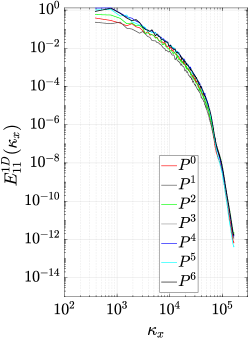
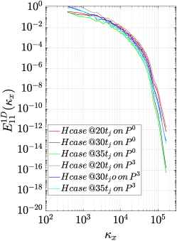
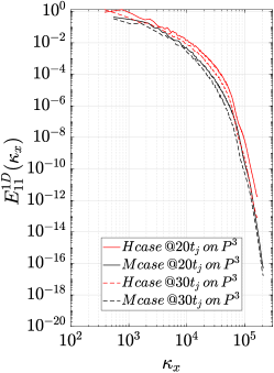
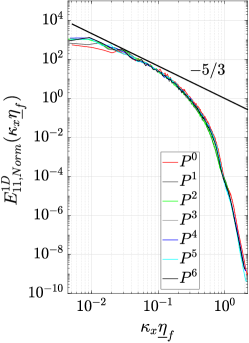
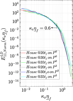
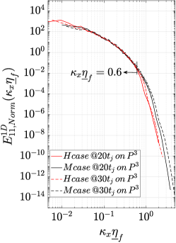
Figure 1: 1D longitudinal velocity spectra across the reacting shear layer. (Top) non-normalized, (bottom) normalized using the Favre averaged $\eta$ and $\varepsilon$. Spectra for (left) case H on different cross planes at $t=20t_{j}$, (middle) for case H on the central and $\underline{Z}_{f}=Z_{st}$ plane and at $t=20,30,35t_{j}$, (right) cases M and H at $t=20,30t_{j}$ on $\underline{Z}_{f}=Z_{st}$ plane.

In near dissipation range, Kraichnan (1959), for non-reactive flows, proposed that the 3D normalized energy spectrum $E_{Norm}$ has an exponential drop-off of the form $E_{Norm}(\kappa\underline{\eta}_{f})=A\left(\kappa\underline{\eta}_{f}\right)^{\alpha}\exp\left(-\beta\left(\kappa\underline{\eta}_{f}\right)^{n}\right)$. The value of $n=1$ is supported by two-point closure theories (Ishihara et al. (2005)) for $\kappa\underline{\eta}_{f}\gg 1$. For near dissipation range (say $0.5\leq\kappa\underline{\eta}_{f}\leq 1.5$) this value is supported by experiments (e.g., Saddoughi & Veeravalli (1994)) and DNS (e.g., Kaneda & Ishihara (2006)). If the compensated form of spectrum (i.e., $E_{Norm}(\kappa\underline{\eta}_{f})\times(\kappa\underline{\eta}_{f})^{5/3}$) is plotted against $\kappa\underline{\eta}_{f}$ in a log-linear plot and if a straight line is observed, it can be concluded that $\alpha=-5/3$ and the slope of the line gives $\beta$. It should be mentioned that we expect a similar functional form of the spectrum (with different $A$) when analysing the 1D velocity spectrum rather than the 3D energy spectrum. This is shown in figure 2. For example for case H (figure 2) in the range of $0.1\leq\kappa_{x}\underline{\eta}_{f}\leq 0.6$ the straight line is observed. However, unlike the well documented slope of $\beta=5.2$ for non-reactive flows (Saddoughi & Veeravalli (1994)), in the near dissipation range, the observed slope is $\beta\approx 7.2$. The same slope can be observed for lower Re case M (see figure 2). The inflection observed before in figure 1 is more evident near $\kappa_{x}\underline{\eta}_{f}\approx 0.8$ for case H in figure 2. Before and after that point, there is a change in the slope. The change of the slope starts from $\kappa_{x}\underline{\eta}_{f}\approx 0.6$ in case H. A change of the slope was previously observed in non-reactive flows however in a very far dissipation range around $\kappa\underline{\eta}\approx 4$ in the DNS of isotropic turbulence with ${Re_{\lambda}}$ range similar to the cases considered here (Martinez et al. (1997)). The spectra computed for case M, which has a higher resolution show the extended range with $\beta=7.2$ slope and the transition occurs at higher normalized wavenumbers, $\kappa_{x}\underline{\eta}_{f}>1.4$ (see figure 2). Different components of the 1D energy spectrum are depicted in figure 2 for case H at $t=20t_{j}$. It is observed that the behaviour of the spectra are consistent with the theory, i.e. $E_{22}\approx E_{33}>E_{11}$, before and after inflection. So it is not clear that if the inflection and change of slope is an intrinsic flame behaviour like what hypothesized in Kolla et al. (2014) for premixed flames (pressure-velocity coupling at laminar flame scales) or is the effect of a tenth order filter which was used in the DNS code. This needs more future investigations. So the focus of our study will be only on the wavenumbers before inflection where the well behaved straight line and the collapse is observed.

The compensated form of the velocity spectra can be used to detect the Kolmogorov constant ${{C_{K}}}$ (Saddoughi & Veeravalli (1994)). Sreenivasan (1995), examined a wide range of experiments for non-reactive flows and suggested a range of $0.53\pm 0.055$ for the 1D Kolmogorov constant. When multiplied by ${55}/{18}$ (see Monin & Yaglom (1971)), it can be transformed to the constant of the 3D spectrum. In this way the value for 3D Kolmogorov’s constant is $1.62\pm 0.17$. Approximately the same value was observed in non-reactive DNS studies (see e.g., Ishihara et al. (2009)). Donzis & Sreenivasan (2010) mentioned that it is difficult to find Kolmogorov’s constant using the compensated form of spectra because a perfectly horizontal region does not exist. A closer inspection also shows that ${{C_{K}}}$ is not a real constant and has a weak ${Re_{\lambda}}$ dependency of about power 0.1 (see e.g. Tsuji (2009)). It can be shown that it is due to the intermittency effects. Intermittency correction can be added to the $\kappa^{5/3}$ power law, however, in low ${Re_{\lambda}}$, the intermittency correction is very low, (order of $10^{-2}$). In the DNS of high ${Re_{\lambda}}$ ($Re_{\lambda}>700$) by Ishihara et al. (2016), the compensated spectrum showed a very short nearly flat region, a tilted region, and a bump near $\kappa\underline{\eta}=0.1$. The bump was also observed in the experiments of Saddoughi & Veeravalli (1994). This is called the bottleneck effect and has been discussed in detail by Donzis & Sreenivasan (2010). Since in the current study the ${Re_{\lambda}}$ is relatively low, the two artefacts will be neglected and $C_{K}$ will be extracted from the compensated spectra. The value of the 1D constant from $E_{11}^{1D}$ is found to be $\approx 0.75$ for the two flames. The value is higher than the reported values for non-reactive jets ($\approx 0.5$).

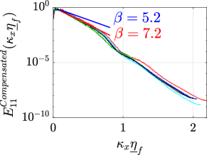
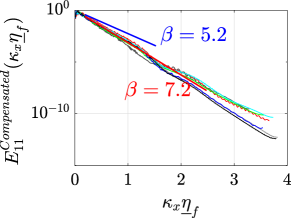
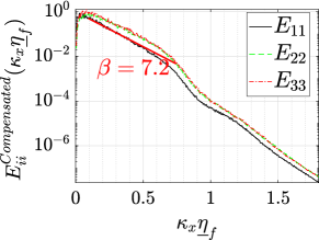
Figure 2: 1D compensated longitudinal spectra at $t=20t_{j}$ for (left) case H, and (middle) case M extracted from different planes across the jets, and (right) case H extracted from the Favre mean Stoichiometric mixture fraction plane. In (a) and (b), the same colors as in figure 1 has been used.

In figure 3 the non-normalised and normalised 1D dissipation spectra are plotted. The normalised 1D dissipation spectrum reads:

$$D_{11,Normal}(\kappa_{x}\underline{\eta}_{f})\equiv\dfrac{D_{11}(\kappa_{x})}{\underline{u_{\eta}}^{3}}=\dfrac{D_{11}(\kappa_{x})}{\underline{\eta}_{f}\underline{\varepsilon}_{f}},$$ (2)

where $D_{11}(\kappa_{x})\equiv 2\underline{\nu}_{f}\kappa_{x}^{2}E_{11}(\kappa_{x})$ with $\underline{\nu}_{f}$ the Favre averaged kinematic viscosity. If one wanted to calculate the 3D TKE ($0.5u_{i}^{\prime\prime}u_{i}^{\prime\prime}$) dissipation spectrum, i.e., $D^{3D}(\kappa)$, it was possible to directly transform the instantaneous dissipation rate, $\varepsilon$, to Fourier space. However, we keep using the conventional incompressible definition and evaluate the 1D dissipation of $u_{1}^{\prime\prime}u_{1}^{\prime\prime}$ instead of $D^{3D}(\kappa)$. It is observed in figure 3 that by approaching the core jet region, the dissipation peak value increases. In the normalized dissipation spectra (the right plot in figure 3), the peak location seems to collapse well and become approximately independent of ${Re_{\lambda}}$ . The peak occurs in $\kappa_{x}\underline{\eta}_{f}\approx 0.08$. This is of great importance. It is observed that the location of the peak of dissipation spectrum in non-premixed flames is lower than the non-reactive jet value and grid generated turbulence reported in Ganapathisubramani et al. (2008) and Saddoughi & Veeravalli (1994), which is $\sim 0.1$. Further, the collapse of the peak location is acceptable when the dissipation spectra are normalized by $\underline{\eta}_{f}$ and $\underline{\varepsilon}_{f}$.

The normalized dissipation spectra are also shown in figure 4 in different conditions. Like before, for case H, up to $\kappa_{x}\underline{\eta}_{f}\approx 0.6$ the collapse is good, while for case M (the case with a higher resolution) the range extends to $\kappa_{x}\underline{\eta}_{f}\approx 1.4$. The spectra extracted from both cases collapsed well up to the point where the change of slope of case H begins (see the right plot in figure 4). It is reasonable to expect that by increasing the resolution of case H, one could see an extended range of the collapse. Nevertheless, it should be considered that the amount of dissipation beyond $\kappa_{x}\underline{\eta}_{f}\approx 0.6$ is low (see the right plot in figure 3).

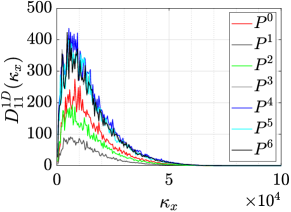
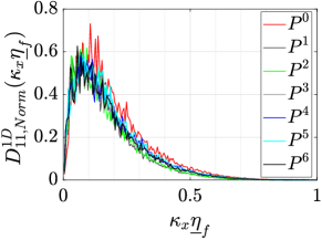
Figure 3: 1D longitudinal dissipation spectra across the reacting shear layer at $t=20t_{j}$ for case H, (left) Non-normalized spectra; (right) Normalized using Favre averaged $\eta$ and $\varepsilon$.

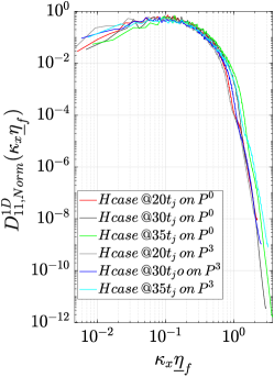
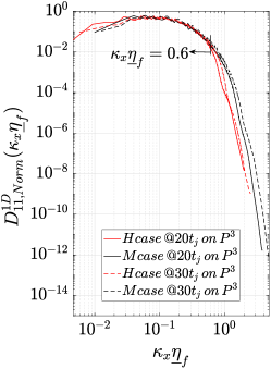
Figure 4: 1D normalized longitudinal dissipation spectra, (left) on different planes and at different times for case H; (right) On $P^{3}$ for cases H and M at different times.

4 Model Spectrum

Pope’s model (Pope (2000)) for the 3D energy spectrum reads:

$$E_{Model,Norm}(\kappa\underline{\eta})=C_{K}\left(\kappa\underline{\eta}\right)^{-5/3}f_{\eta}(\kappa\underline{\eta})f_{L}(\kappa L),$$ (3)

The model has been proposed for constant density flows and includes the Kolmogorov spectrum for the inertial range, an integral range multiplier, $f_{L}(\kappa L)$, for low and a dissipation range multiplier, $f_{\eta}(\kappa\underline{\eta})$ for high wavenumbers. In the current work, the conventional form of $f_{L}(\kappa L)$, viz. $f_{L}(\kappa L)=(\dfrac{\kappa L}{(\left(\kappa L\right)^{2}+c_{L})^{1/2}})^{5/3+P_{0}}$, with same coefficients as non-reactive flows, i.e., $P_{0}=2$ and $c_{L}=6.78$ will be used since the wavenumber ranges of interest are the inertial and near dissipative ranges. Pope proposed $f_{\eta}(\kappa\underline{\eta})$ as:

$$f_{\eta}(\kappa\underline{\eta})=exp[-\beta\left(\left(\kappa\underline{\eta}\right)^{4}+c_{\eta}^{4}\right)^{1/4}-c_{\eta}],$$ (4)

with experimentally obtained constants of $\beta=5.2$ (Saddoughi & Veeravalli (1994)) and $c_{\eta}=0.4$. As shown in the previous section we found a steeper exponential drop-off with $\beta\approx 7.2$. The 3D model energy spectrum must be converted to a 1D spectrum to be compared to, e.g., $E_{11}$. If isotropy is assumed, one can derive the 1D velocity (e.g., streamwise) spectrum from the 3D energy spectrum (Monin & Yaglom (1971)):

$$E_{11,Model}^{1D}(\kappa_{x})=\int_{\kappa_{x}}^{\infty}\left(1-\dfrac{\kappa_{x}^{2}}{\kappa^{2}}\right)\dfrac{E_{Model}(\kappa)}{\kappa}d\kappa$$ (5)

The dissipation spectrum reported in linear scales (figure 5) shows interesting features. In this figure, five different normalized velocity dissipation spectra are plotted. The black line with circle markers is the 3D dissipation model of Pope with its peak at $\kappa\underline{\eta}_{f}\approx 0.26$. It is clear that the 1D dissipation spectrum of stream-wise velocity fluctuations (the black dashed line) does not follow the model. The 1D form of the model computed by Eq. 5 and plotted in green with triangle markers is the one that should be compared with the DNS. The peak of the 1D model dissipation spectrum occurs at $\kappa_{x}\underline{\eta}_{f}\approx 0.11$. This value is in agreement with the observations in experiments (e.g. Saddoughi & Veeravalli (1994)) and DNS (Ganapathisubramani et al. (2008)) of non-reactive flows. However, it is observed that the peak of the 1D dissipation spectrum of the non-premixed jet flames considered in this study is at a lower wavenumber ($\kappa_{x}\underline{\eta}_{f}\approx 0.08$). Approximately the same value was observed in the DNS of premixed flames (see figure 9 in Kolla et al. (2016)). The red line is an adapted 1D model using the observed $C_{K}^{1D}\approx 2.3$, $\beta\approx 7.2$ and fitted $c_{\eta}=0.28$. Finally, if the 3D model is plotted using these new coefficients, the result is the blue line with cross markers. The peak of the new 3D model is at $\kappa\underline{\eta}_{f}\approx 0.19$ instead of $\kappa\underline{\eta}_{f}\approx 0.26$. Further, it is less extended to the far dissipation range ($\kappa\underline{\eta}_{f}>1$). Note that the areas under the two curves are equal.

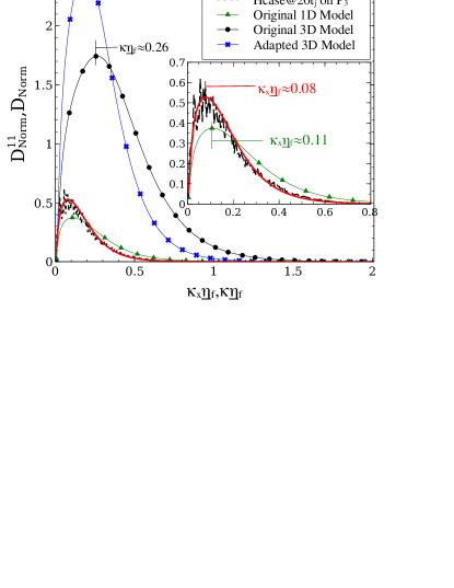
Figure 5: Different dissipation spectra on $\underline{Z}_{f}=Z_{st}$ plane at $t=20t_{j}$ for case H compared to model spectra. The inset is the zoom view of the left corner.

5 Summary and Conclusions

In this study the velocity and its dissipation spectra in non-premixed jet flames were analysed using two DNS databases of temporally evolving syngas jet flames experiencing high levels of local extinction followed by re-ignition. In each database, three different times were selected (6 in total) corresponding to the events of maximum local extinction and re-ignition. Consistent with Knaus & Pantano (2009) (non-premixed jet flames DNS) and Kolla et al. (2014) (premixed jet flames DNS), it was observed that using Favre averaged Kolmogorov’s length scale and energy dissipation rate, namely $\underline{\eta}_{f}$ and $\underline{\varepsilon}_{f}$, the velocity spectra calculated on different planes across the reacting shear layers and in different flame dynamics, collapse very well on a curve in the inertial and near dissipation ranges before the discussed inflection occurs. The $\kappa^{-5/3}$ power law was observed in the inertial range, with the constant of proportionality of $C_{K}=2.3$ instead of $1.5$. In the dissipation range, the exponential drop-off factor of the spectra is steeper than the corresponding non-reactive flows. It was observed that $\exp(\beta\kappa)$ scaling exists with $\beta=7.2$ instead of $\beta=5.2$. The 1D dissipation spectra do not follow the standard 1D model dissipation spectrum. Keeping the functional form of the model unchanged and using the observed values of $C_{K}=2.3$, $\beta=7.2$, and a fitting value of $c_{\eta}=0.28$, the agreement of the model spectrum and the dissipation spectra from DNS is highly improved. Future works will focus on extending the investigations on the drop-off factor, using reactive DNS databases with higher Re and higher resolutions. It is of interest to see if $\beta=7.2$ is a common behaviour in reactive jets or not. Moreover, using larger datasets, one may improve the fitting of $c_{\eta}$. The outcomes of this study can be applied in the modelling of turbulent reactive flows, either in turbulence modelling (e.g. for RANS/LES) or combustion modelling (e.g. EDC model of Ertesvåg & Magnussen (2000)).

This work has received funding from the European Union’s Horizon 2020 research and innovation programme under the Marie Sklodowska-Curie grant agreement No 643134. We would like to thank Professor Evatt Hawkes from The University of New South Wales for providing us the DNS databases and also Professor Dominique Thévenin from the University of Magdeburg and Dr. Christiane Zistl to provide us ANAFLAME codes.

References

- Attili & Bisetti (2013) Attili, Antonio & Bisetti, Fabrizio 2013 Fluctuations of a passive scalar in a turbulent mixing layer. Physical Review E 88 (3), 033013.
- Batchelor (1959) Batchelor, George K 1959 Small-scale variation of convected quantities like temperature in turbulent fluid part 1. general discussion and the case of small conductivity. Journal of Fluid Mechanics 5 (1), 113–133.
- Donzis & Sreenivasan (2010) Donzis, DA & Sreenivasan, KR 2010 The bottleneck effect and the kolmogorov constant in isotropic turbulence. Journal of Fluid Mechanics 657, 171–188.
- Donzis et al. (2010) Donzis, Diego A, Sreenivasan, KR & Yeung, PK 2010 The batchelor spectrum for mixing of passive scalars in isotropic turbulence. Flow, turbulence and combustion 85 (3-4), 549–566.
- Ertesvåg & Magnussen (2000) Ertesvåg, Ivar S & Magnussen, Bjørn F 2000 The eddy dissipation turbulence energy cascade model. Combustion science and technology 159 (1), 213–235.
- Fuest et al. (2018) Fuest, Frederik, Barlow, Robert S, Magnotti, Gaetano & Sutton, Jeffrey A 2018 Scalar dissipation rates in a turbulent partially-premixed dimethyl ether/air jet flame. Combustion and Flame 188, 41–65.
- Ganapathisubramani et al. (2008) Ganapathisubramani, B, Lakshminarasimhan, K & Clemens, NT 2008 Investigation of three-dimensional structure of fine scales in a turbulent jet by using cinematographic stereoscopic particle image velocimetry. Journal of fluid mechanics 598, 141–175.
- Hawkes et al. (2007) Hawkes, Evatt R, Sankaran, Ramanan, Sutherland, James C & Chen, Jacqueline H 2007 Scalar mixing in direct numerical simulations of temporally evolving plane jet flames with skeletal co/h2 kinetics. Proceedings of the combustion institute 31 (1), 1633–1640.
- Ishihara et al. (2009) Ishihara, Takashi, Gotoh, Toshiyuki & Kaneda, Yukio 2009 Study of high–reynolds number isotropic turbulence by direct numerical simulation. Annual Review of Fluid Mechanics 41, 165–180.
- Ishihara et al. (2005) Ishihara, Takashi, Kaneda, Yukio, Yokokawa, Mitsuo, Itakura, Ken’ichi & Uno, Atsuya 2005 Energy spectrum in the near dissipation range of high resolution direct numerical simulation of turbulence. Journal of the Physical Society of Japan 74 (5), 1464–1471.
- Ishihara et al. (2016) Ishihara, Takashi, Morishita, Koji, Yokokawa, Mitsuo, Uno, Atsuya & Kaneda, Yukio 2016 Energy spectrum in high-resolution direct numerical simulations of turbulence. Physical Review Fluids 1 (8), 082403.
- Kaneda & Ishihara (2006) Kaneda, Yukio & Ishihara, Takashi 2006 High-resolution direct numerical simulation of turbulence. Journal of Turbulence (7), N20.
- Knaus & Pantano (2009) Knaus, R & Pantano, C 2009 On the effect of heat release in turbulence spectra of non-premixed reacting shear layers. Journal of Fluid Mechanics 626, 67–109.
- Kolla et al. (2014) Kolla, H, Hawkes, ER, Kerstein, AR, Swaminathan, Nedunchezhian & Chen, JH 2014 On velocity and reactive scalar spectra in turbulent premixed flames. Journal of Fluid Mechanics 754, 456–487.
- Kolla et al. (2016) Kolla, Hemanth, Zhao, Xin-Yu, Chen, Jacqueline H & Swaminathan, N 2016 Velocity and reactive scalar dissipation spectra in turbulent premixed flames. Combustion Science and Technology 188 (9), 1424–1439.
- Kraichnan (1959) Kraichnan, Robert H 1959 The structure of isotropic turbulence at very high reynolds numbers. Journal of Fluid Mechanics 5 (4), 497–543.
- Kraichnan (1968) Kraichnan, Robert H 1968 Small-scale structure of a scalar field convected by turbulence. The Physics of Fluids 11 (5), 945–953.
- Martinez et al. (1997) Martinez, DO, Chen, S, Doolen, GD, Kraichnan, RH, Wang, L-P & Zhou, Y 1997 Energy spectrum in the dissipation range of fluid turbulence. Journal of plasma physics 57 (1), 195–201.
- Monin & Yaglom (1971) Monin, A.S. & Yaglom, A.M. 1971 Statistical fluid mechanics: mechanics of turbulence. Statistical Fluid Mechanics: Mechanics of Turbulence v. 1. MIT Press.
- Petersen & Ghandhi (2011) Petersen, Ben & Ghandhi, Jaal 2011 High-resolution turbulent scalar field measurements in an optically accessible internal combustion engine. Experiments in fluids 51 (6), 1695–1708.
- Pope (2000) Pope, S.B. 2000 Turbulent Flows. Cambridge University Press.
- Saddoughi & Veeravalli (1994) Saddoughi, Seyed G & Veeravalli, Srinivas V 1994 Local isotropy in turbulent boundary layers at high reynolds number. Journal of Fluid Mechanics 268, 333–372.
- Sreenivasan (1995) Sreenivasan, Katepalli R 1995 On the universality of the kolmogorov constant. Physics of Fluids 7 (11), 2778–2784.
- Sreenivasan (1996) Sreenivasan, Katepalli R 1996 The passive scalar spectrum and the obukhov–corrsin constant. Physics of Fluids 8 (1), 189–196.
- Tsuji (2009) Tsuji, Yoshiyuki 2009 High-reynolds-number experiments: the challenge of understanding universality in turbulence. Fluid dynamics research 41 (6), 064003.
- Wang & Barlow (2008) Wang, Guanghua & Barlow, Robert S 2008 Spatial resolution effects on the measurement of scalar variance and scalar gradient in turbulent nonpremixed jet flames. Experiments in Fluids 44 (4), 633–645.
- Wang et al. (2007a) Wang, Guanghua, Karpetis, Adonios N & Barlow, Robert S 2007a Dissipation length scales in turbulent nonpremixed jet flames. Combustion and Flame 148 (1-2), 62–75.
- Wang et al. (2007b) Wang, G-H, Barlow, Robert S & Clemens, Noel T 2007b Quantification of resolution and noise effects on thermal dissipation measurements in turbulent non-premixed jet flames. Proceedings of the Combustion Institute 31 (1), 1525–1532.
- Warhaft (2000) Warhaft, Zellman 2000 Passive scalars in turbulent flows. Annual Review of Fluid Mechanics 32 (1), 203–240.
- Yeung & Sreenivasan (2013) Yeung, PK & Sreenivasan, KR 2013 Spectrum of passive scalars of high molecular diffusivity in turbulent mixing. Journal of Fluid Mechanics 716.