Abstract Transducers

Abstract.

Several abstract machines that operate on symbolic input alphabets have been proposed in the last decade, for example, symbolic automata or lattice automata. Applications of these types of automata include software security analysis and natural language processing. While these models provide means to describe words over infinite input alphabets, there is no considerable work on symbolic output (as present in transducers) alphabets, or even abstraction (widening) thereof. Furthermore, established approaches for transforming, for example, minimizing or reducing, finite-state machines that produce output on states or transitions are not applicable. A notion of equivalence of this type of machines is needed to make statements about whether or not transformations maintain the semantics.

We present abstract transducers as a new form of finite-state transducers. Both their input alphabet and the output alphabet is composed of abstract words, where one abstract word represents a set of concrete words. The mapping between these representations is described by abstract word domains. By using words instead of single letters, abstract transducers provide the possibility of lookaheads to decide on state transitions to conduct. Since both the input symbol and the output symbol on each transition is an abstract entity, abstraction techniques can be applied naturally.

We apply abstract transducers as the foundation for sharing task artifacts for reuse in context of program analysis and verification, and describe task artifacts as abstract words. A task artifact is any entity that contributes to an analysis task and its solution, for example, candidate invariants or source code to weave.

1. Introduction

Figure 1. Each transition of an abstract transducer is annotated with an abstract input word $\mathfrak{v}$ and an abstract output word ${\mathfrak{w}}$. An abstract input word denotes $[\![\mathfrak{v}]\!]\subseteq\Sigma^{*}$ a set of words over an input alphabet $\Sigma$, an abstract output word denotes $[\![{\mathfrak{w}}]\!]\subseteq\Theta^{\infty}$ a set of words over an output alphabet $\Theta$; the illustration shows the sets of concrete words. Please note that already the activation of the initial state $q_{0}$ emits an abstract output word—in this case: the set $\{\texttt{p}\}$ of concrete words. We use the abstract epsilon word $\mathfrak{v}_{\epsilon}$, with $[\![\mathfrak{v}_{\epsilon}]\!]=\{\epsilon\}$, with the semantics that is known from $\epsilon$-NFAs (Hopcroft et al., 2003; Sipser, 1997). Transitions with the abstract input word $\mathfrak{v}_{\epsilon}$ are called $\epsilon$-moves and can result in output words of infinite length, which result from $\epsilon$-loops—for example, the loop $q_{2}\smash{\stackrel{{\scriptstyle}}{{\rightarrow}}}q_{3}\smash{\stackrel{{\scriptstyle}}{{\rightarrow}}}q_{4}\smash{\stackrel{{\scriptstyle}}{{\rightarrow}}}q_{2}$. The table on the right shows—for the transducer on the left—a set of input words and corresponding output words in the form of regular expressions.

We present abstract transducers as a new type of abstract machines that operate on an abstract input alphabet and an abstract output alphabet, and that have an inherent notion of abstraction. Both the input alphabet and the output alphabet are described based on abstract domains, which enables different forms of abstracting these transducers and allows for different forms of symbolic representations. An abstract representation of words is essential for creating finite abstractions of possibly exponentially many and infinitely long output words, and abstraction of a transducer allows to increase the sharing of its outputs, that is, one output becomes applicable to a wider set of input words. Different abstract domains, and respective lattices, have been proposed to represent and abstract states and behaviors of systems and their relationships (Cousot and Cousot, 1977). An abstract domain provides means to map between abstract and concrete entities. Combining abstract domains and finite-state transducers results in a generic formalism that provides a unified view on different types of automata and transducers, and enables new applications in different areas, for example, in program analysis and verification. Figure 1 illustrates the working principle of abstract transducers.

Problems.

Abstract transducers address several problems: (1) In case alphabets consist of many, possibly exponentially many, symbols, traditional automata concepts with single concrete symbols per transitions provide limited efficiency. Automata that employ a symbolic alphabet—where one symbol from the alphabet denotes a set of concrete symbols—solve this issue (van Noord and Gerdemann, 2001; Veanes, 2013). Having a symbolic representation of alphabet symbols makes approaches for abstracting (or widening) finite-state machines—such as relational abstraction or alphabet abstraction (Bultan et al., 2017; Preda et al., 2015)—applicable. We use abstract domains, as known from abstract interpretation, for constructing symbolic representations, and mapping between concrete and symbolic alphabets. This way, we can choose from a large variety of abstract domains to provide different symbolic and explicit mechanisms for representing data, for example, binary decision diagrams (Bryant, 1992), predicates (Graf and Saïdi, 1997; Ball et al., 2001b), or polyhedra (Singh et al., 2017). Abstraction is also essential for output words, which are produced by transducers, and has not yet received attention by researchers. (2) We allow the transducers to have $\epsilon$-moves that are annotated with outputs, which can lead to output words of infinite length; here, a symbolic representation of sets of output words, based on corresponding abstract domains for the output alphabet, can help to provide a finite representation that represents or even overapproximates sets of exponentially many and infinitely long words. By having a means for abstracting both the input alphabet and the output alphabet, we can implement further, more elaborated techniques with various applications. We abstract our transducers to increase the sharing of the output they emit. An abstract transducer might have been constructed to produce its output for a specific set of input words that can be found in a specific analysis task, that is, (3) the reuse of the output can be limited to a specific set of analysis tasks, while the output would also be applicable to a broader set of tasks. Sharing is increased if a given output word becomes produced for a larger set of input words—that is, we take advantage of the nondeterminism that abstraction introduces (Avni and Kupferman, 2013). The alphabets from that these words can be composed of can (in general) consist of arbitrarily complex entities (symbols), for example, tuples of concrete letters as used for multi-track automata (Bultan et al., 2017). (4) Nevertheless, also for these complex symbols, a means of abstraction is needed. Constructing complex alphabets, and words thereof, based on abstract product domains (Cortesi et al., 2013) addresses this issue.

(a) Yarn Transducer

(b) Precision Transducer

Figure 2. Two types of abstract transducers are illustrated: A Yarn transducer that emits code to weave, that is, it corresponds to an aspect in AOP, and a precision transducer, which is a means to share candidate invariants, or predicates, for (re-)use in predicate abstraction. Please note that the abstract input word $\mathfrak{v}_{3}$ describes a lookahead, that is, it contains a word $\bar{\sigma}\in[\![\mathfrak{v}]\!]$ with $|\bar{\sigma}|>1$. The lookahead matches if the input that remains to be consumed after word $\mathfrak{v}_{3}$ matched starts with alloc($1,$2), where $1 and $2 are parameters that bind the arguments that are given to the function alloc to internal variables, which are then used to produce the concrete output for the abstract output words ${\mathfrak{w}}_{1}$ and ${\mathfrak{w}}_{2}$.

Applications.

We instantiate abstract transducers as task artifact transducers. A task artifact transducer is an abstract transducer that maps between a set of control paths of a given program to analyze and a set of task artifacts, which are intended to be shared for reuse. Task artifact transducers are a generic means to provide artifacts that contributes to an analysis task and its solution. These task artifact transducers aid in various analysis tasks for that task artifacts, for example, intermediate verification results, have to be provided at specific points and in specific contexts in the control flow. By using such transducers as means for sharing artifacts for reuse, we gain precise control over the sharing process: We can precisely specify at which points and in which context (path prefix), of the control flow of a program, certain artifacts should be shared for reuse. We use them both to construct the transition relation of the analysis task itself, and for constructing a state-space abstraction with a finite number of abstract states in an efficient and effective manner, that is, for sharing syntactic and semantic task artifacts. Syntactic task artifacts include, for example, components, aspects, or assertions to check (Kiczales et al., 1997; Ball and Rajamani, 2002). Semantic task artifacts include, for example, function summaries (Sery et al., 2012), invariants, or Craig interpolants (Henzinger et al., 2002, 2004). The goal of sharing task artifacts is to make the overall process of constructing syntactic and semantic task models more efficient and effective.

We present two forms of task artifact transducers based on abstract transducers in another work (Stahlbauer, 2019): Yarn transducers and precision transducers. Figure 2 provides examples for these types of abstract transducers. A Yarn transducer can express aspects—source code, or labeled transition systems (LTSs) in general, to emit at specific points—to weave into a control-flow graph. Such aspects can, for example, provide the environment model or a specification. It must be possible to emit code to weave before any of the transitions that are processed as input: An initial transducer output is needed. For soundness, operations such as $\epsilon$-elimination, union, or reduction must keep the semantics—including their temporal relationships, also concurrency—of these aspects. A precision transducer is annotated with sets of predicates (candidate invariants) to emit for reuse in different contexts of the transition system to construct (for example, a Kripke structure) in an analysis process. The shared predicates can be used to compute predicate abstractions (as used for software model checking (Graf and Saïdi, 1997; Ball et al., 2001a)), the number of CEGAR (Clarke et al., 2000; Beyer et al., 2013b) iterations can be reduced by abstracting these transducers, which increases sharing (the same predicate can be emitted in more contexts). Such precision transducers can also express the predicate sharing strategy of lazy abstraction (Henzinger et al., 2002).

1.0.1. Contributions

This work presents the following contributions and shares most of the material with the author’s thesis (Stahlbauer, 2019):

• Abstract Transducers. We introduce abstract transducers as a generic and unifying type of abstract machines that use abstract word domains to characterize both the input alphabet and the output alphabet, and that have an inherent notion of abstraction.

• Abstract Output Closure. We present techniques for computing finite abstractions of the output of $\epsilon$-closures with $\epsilon$-loops, which are possible if $\epsilon$-moves are allowed. These techniques allow to produce finite outputs from transducers with outputs that describe exponentially large sets of potentially infinitely long words, and they aid in eliminating the $\epsilon$-moves.

• Transducer Abstraction. We exactly define what it means to abstract (or overapproximate) an abstract transducer. Based on this notion of abstraction we discuss different types of abstractions and define corresponding operators.

• Transducer Reduction. After defining the notion of equivalence of abstract transducers, we discuss different transformations that maintain their semantics while reducing their number of control states and transitions. Such reduction techniques help to reduce the degree of non-determinism, which reduces the costs of executing abstract transducers.

• Transducer Analysis. We present an abstract transducer analysis as a generic configurable program analysis for running different types of abstract transducers.

• Task Artifact Transducers. We instantiate abstract transducers as task artifact transducers to have a generic means to share various artifacts that contribute to different concerns of an analysis task. Task artifact transducers foster the reuse of components of an analysis task and the intermediate analysis (reasoning) results that are produced while conducting an analysis.

1.0.2. Key Insights

(1) Abstract transducers have a fundamentally different semantic compared to other transducers with symbolic alphabets, such as symbolic transducers (D’Antoni and Veanes, 2017b), which becomes obvious when comparing their notions of equivalence. (2) Existing algorithms for transforming finite-state transducers are not applicable for abstract transducers. (3) Abstracting abstract transducers is a means for systematically increasing the scope of sharing artifacts for reuse.

2. Preliminaries

We start with preliminaries, including the notation: We denote sets $A,B,\ldots$ by upper case letters or add a hat $\widehat{a},\widehat{b},\ldots$ to signal that an entity is a set. Set elements $a,b,\ldots$ are denoted by lower case letters. We add a bar $\bar{a},\bar{B},\ldots$ to denote lists (or sequences). Elements of sets are enclosed $\{a,b,c\}$ in curly brackets, components of tuples are enclosed $(A,x,y)$ in round brackets, elements of lists are enclosed $\langle a,b,c\rangle$ in angle brackets.

2.0.1. Languages and Words

The set of all finite words over an alphabet $\Sigma$ is denoted by $\Sigma^{*}$, which is a free monoid $\Sigma^{*}=(\Sigma,\circ,\epsilon)$, also known as Kleene star, where concatenation $\circ:\Sigma^{*}\times\Sigma^{*}\rightarrow\Sigma^{*}$ is its binary operator and its neutral element $\epsilon$ is the empty word. A word $\bar{\sigma}$ is a sequence $\langle\sigma_{1},\ldots,\sigma_{n}\rangle$ of symbols from the alphabet. The length $|\bar{\sigma}|$ of a word $\bar{\sigma}$ is its number of subsequent symbols; the empty word has length $|\epsilon|=|\langle\rangle|=0$. Given two words $\bar{\sigma}=\langle\sigma_{1},\ldots,\sigma_{n}\rangle$ and $\bar{\tau}=\langle\tau_{1},\ldots,\tau_{m}\rangle$, the concatenation $\bar{\sigma}\circ\bar{\tau}$ results in the word $\bar{c}=\langle\sigma_{1},\ldots,\sigma_{n},\tau_{1},\ldots,\tau_{m}\rangle$ with length $|\bar{c}|=|\bar{\sigma}|+|\bar{\tau}|$. A word $\bar{\sigma}_{a}$ is prefix of another word $\bar{\sigma}_{b}$, that is, it is element $(\bar{\sigma}_{a},\bar{\sigma}_{b})\in\preceq$ of the prefix relation $\preceq$, if there exists a suffix $\bar{\sigma}_{s}\in\Sigma^{*}$ such that $\bar{\sigma}_{b}=\bar{\sigma}_{a}\circ\bar{\sigma}_{s}$. While the finitely words over an alphabet $\Sigma$ are denoted by $\Sigma^{*}$, the infinitely long ones are denoted by $\Sigma^{\omega}$, and the set of all words is denoted by $\Sigma^{\infty}=\Sigma^{*}\cup\Sigma^{\omega}$ (Löding and Tollkötter, 2016), with the infinite iteration $\cdot^{\omega}$ and the finite iteration $\cdot^{*}$. The set of all words over an alphabet $\Sigma$ that is described by a structure $S$ and that are considered well-formed regarding certain production rules is called language $\mathcal{L}(S)\subseteq\Sigma^{*}$ of $S$. The empty word language $\{\epsilon\}$ consists of the empty word $\epsilon$ only, the empty language corresponds to the empty set $\emptyset$.

2.0.2. Lattices

A (complete) lattice (Grätzer, 2011) is a tuple $\dddot{E}=(E,\sqsubseteq,\sqcap,\sqcup,\top,\bot)$, with a set of abstract elements $E$ and a partial order relation $\sqsubseteq\;\subseteq E\times E$. The operator meet is a relation $\sqcap:(E\times E)\rightarrow E$ that provides the greatest lower bound for a given pair $(e_{1},e_{2})\in E\times E$ of abstract elements. The operator join is a relation $\sqcup:E\times E\rightarrow E$ that provides the least upper bound for a given pair of abstract elements. The bottom element $\bot$ is the least element in the partial order relation, that is, there exists no other element $e\sqsubseteq\bot$, with $e\neq\bot$. The top element $\top$ is the greatest element in the partial order, that is, there exists no other element $\top\sqsubseteq e$, with $e\neq\top$. The operators $\sqcap$ and $\sqcup$ extend to sets naturally: The meet over a set of abstract elements is denoted by $\bigsqcap:2^{E}\times E$, and the join by $\bigsqcup:2^{E}\times E$, for example, $\bot=\bigsqcap E$ and $\top=\bigsqcup E$. A semi lattice either has no meet or no join for all abstract elements. The relation $\sqsubseteq$ is also called the inclusion relation (Whitman, 1946). Partial ordered sets (posets) can be made semi-lattices, and semi-lattices can be made complete by adding additional abstract elements (Garg, 2015). A lattice element $e_{c}\in E$ is called complement of an element $e\in E$ iff $e\sqcap e_{c}=\bot$ and $e\sqcup e_{c}=\top$. We denote the complement of an lattice element $e$ by $\lnot e$. A lattice is called complemented iff there exists a complement for all its elements.

2.0.3. Powerset Lattice

The powerset lattice that describes a Hoare powertheory (Abramsky et al., 1994; Ferguson and Hughes, 1989; Hart and Tsinakis, 2007)—over a given lattice $\dddot{E}=(E,\sqsubseteq_{E},\sqcap_{E},\sqcup_{E},\top_{E},\bot_{E})$—is denoted by $\mathsf{pw}(\dddot{E})=(2^{E},\sqsubseteq,\sqcap,\sqcup,\top,\bot)$, where the set of elements is constituted by the set of all subsets $2^{E}$ of set $E$. The inclusion relation $\sqsubseteq$ has the element $(E_{1},E_{2})\in\sqsubseteq$ if and only if $\forall e_{1}\in E_{1}\exists e_{2}\in E_{2}:e_{1}\sqsubseteq_{E}e_{2}$. The join $\sqcup(E_{1},E_{2})=E_{1}\cup E_{2}$ is the union, and the meet $\sqcap(E_{1},E_{2})=E_{1}\cap E_{2}$ is the intersection of two given sets $E_{1},E_{2}\subseteq E$. The bottom element $\bot=\emptyset$ is the empty set, and the top element $\top=E$ corresponds to the set with all elements.

Any complemented distributive lattice is isomorphic to a Boolean algebra (Huntington, 1904), which also follows from the Stone duality (Stone, 1936); one example for such lattices are powerset lattices. Lattices generalize Boolean algebras by not requiring complement and distributivity in the first hand.

2.0.4. Map Lattice

A map lattice $\mathsf{ml}(K,\dddot{V})=(2^{K\rightarrow V},\sqsubseteq,\sqcap,\sqcup,\top,\bot)$ is a lattice of elements that are maps, that is, the elements are functions that map from a set $K$ of keys to a set $V$ of values; the values of this map are elements of another lattice $\dddot{V}=(V,\sqsubseteq_{V},\sqcap_{V},\sqcup_{V},\top_{V},\bot_{V})$. Such a lattice are also known as function lattice (Duffus et al., 1978; Back and von Wright, 1990). The inclusion relation $\sqsubseteq$ has element $(m_{1},m_{2})\in\sqsubseteq$ if and only if $\forall k\in K:m_{1}(k)_{\bot}\sqsubseteq_{V}m_{2}(k)_{\bot}$. In the following, we rely on the function $m(k)_{\bot}=m(k)\;\text{if}\;(k,\cdot)\in m\;\text{otherwise}\;\bot_{V}$ which returns the value for a given key $k$ from a map $m$, and the bottom element of the value lattice if no entry for the key is present. The meet $\sqcap$ is defined by $\sqcap(m_{1},m_{2})=\{(k,v_{1}\sqcap_{V}v_{2})\,|\,(k,v_{1})\in m_{1}\land v_{2}=m_{2}(k)_{\bot}\}$, the join $\sqcup$ is defined by $\sqcup(m_{1},m_{2})=\{(k,m_{1}(k)_{\bot}\sqcup_{V}m_{2}(k)_{\bot})\,|\,k\in\textsf{keys}(m_{1})\cup\textsf{keys}(m_{2})\}$, the top element $\top$ is defined by $\top=\{(k,\top_{V})\,|\,k\in K\}$, and the bottom element $\bot$ is defined by $\bot=\{(k,\bot_{V})\,|\,k\in K\}$.

We define an image-join operator $\bigsqcup_{\rightarrow}:2^{K\times E}\rightarrow 2^{K\rightarrow E}$: Given a map $M\subseteq K\times E$, with a set of keys $K$, and a set of lattice elements $E$, the operator joins all tuples $(k,e)\in M$ with the same key $k$ into one tuple with a value that aggregates all value elements $e$, that is, $\bigsqcup_{\rightarrow}M=\{\;(k,\bigsqcup\,\{e\;|\;e\in\{(k,e)\in M\}\})\;|\;k\in\{k\;|\;(k,\cdot)\in M\}\;\}$.

2.0.5. Abstract Domains

An abstract domain $D=(\dddot{C},\dddot{E},[\![\cdot]\!],\langle\!\langle\cdot\rangle\!\rangle)$ (Cousot and Cousot, 1992) is defined based on a tuple that consists of a lattice $\dddot{C}$ of the set of concrete elements $C$, a lattice $\dddot{E}$ of the set of abstract elements $E$, a denotation function $[\![\cdot]\!]$ and an abstraction function $\langle\!\langle\cdot\rangle\!\rangle$. The set $C$ consists of all possible interpretations of elements from the set of abstract elements $E$ for a specific universe. The denotation $[\![e]\!]:E\rightarrow 2^{C}$ of an abstract element $e$ is the set of all its possible interpretations—as known from denotational semantics (Abramsky et al., 1994). The abstraction $\langle\!\langle e\rangle\!\rangle$ of an abstract element $e$ results in a new abstract element $e^{\prime}$ with $[\![e]\!]\subseteq[\![e^{\prime}]\!]$. The abstraction $\langle\!\langle C_{k}\rangle\!\rangle$ of a set of concrete elements $C_{k}\subseteq C$ results in an abstract element $e$, with $[\![e]\!]=C_{k}$. An abstraction $\langle\!\langle\cdot\rangle\!\rangle^{\pi}$ with widening produces an abstraction with an abstraction precision $\pi$, which can result in a widening. The abstraction precision $\pi\in\Pi$ (Nayak and Levy, 1995) defines the set of details that the resulting abstraction should maintain for sound reasoning. Two elements are called semantically equal, that is, $e_{1}\equiv e_{2}$, if and only if $[\![e_{1}]\!]=[\![e_{2}]\!]$ in the same universe. One element semantically implies another element, that is, $e_{1}\vDash e_{2}$, if and only if $[\![e_{1}]\!]\subseteq[\![e_{2}]\!]$.

3. Abstract Words

Before we present abstract transducers, we describe concepts to cope with sets of possibly exponentially many and infinitely long words symbolically. A word can express temporal or causal relationships between the letters of the word. We introduce concepts and techniques to deal with sets of words on an abstract level.

3.1. Hierarchy of Characters, Words, and Languages

We now discuss established terms that are relevant in the context of the terms that we introduce in the following sections. This helps to understand our terminology choices.

Both the input alphabet and the output alphabet of an abstract transducer is characterized based on an abstract domain. Abstract domains are a generic means for abstraction and provide various operations for manipulating and comparing abstract elements (entities) (Cousot and Cousot, 1977), and for mapping between concrete and abstract elements.

Elements from a set $\Sigma$ can be combined to form (possibly infinite) sequences $\bar{\sigma}\in\Sigma^{\infty}$ of those elements. We use the term word to denote sequences of elements that can be formed from other words by concatenation. Words are elements of a free monoid (semigroup) for that concatenation is the binary and associative operator, and the empty word (empty sequence) is the identity (neutral) element. A language is a set of words—and typically well-formed regarding some production rules.

In a generic abstract domain, one abstract element maps to a set of concrete elements, which is reflected by the denotation (concretization) function $[\![\cdot]\!]$. That is, we can deduce that one abstract word represents a set of concrete words, and an abstract language maps to a set of concrete languages.

A word, as mentioned earlier, establishes a temporal relationship between all its characters; each character has a semantic denotation on its own, that is, it maps to a set of entities. The expressiveness of words compared their characters is dual to the expressiveness of linear temporal logic to propositional logic: A formula in propositional logic (interpreted for a specific universe) denotes a set of entities, whereas a formula in linear temporal logic denotes sequences of sets of entities (over time). A set of words, that is, a language, provides sufficient expressiveness to describe a set of forks in words over time, for example, to describe a set of concurrent program executions, or for matching trees or (more general) graphs.

That is, an abstract word, which maps to a set of concrete words, provides an abstraction with sufficient expressiveness to describe sets of linear-time concerns, and an abstract language, which represents a set of sets of words, provides expressiveness to describe sets of concerns that are expressible in branching-time logic. In the following, we restrict the discussion and presentation to abstract words and keep abstract languages for future work.

3.2. Abstract Word Domain

The foundation of abstract transducers is formed by the abstract word domain, a lattice-based abstract domain (Cousot and Cousot, 1977; Filé et al., 1996) for mapping between abstract words and concrete words.

Definition 3.1 (Abstract Word).

An abstract word $\mathfrak{v}\in\mathfrak{I}$ is a symbolic representation of a set $\subseteq\Sigma^{\infty}$ of concrete words over a concrete alphabet $\Sigma$, where the set $\mathfrak{I}$ denotes all abstract words.

The relationship between an abstract word and the set of concrete words it represents, along with a means for abstraction, is defined by the abstract word domain:

Definition 3.2 (Abstract Word Domain).

An abstract word domain is an abstract domain $D_{W}=(\mathsf{pw}(\dddot{W}),\dddot{\mathfrak{I}},\allowbreak[\![\cdot]\!],\allowbreak\langle\!\langle\cdot\rangle\!\rangle)$ that has abstract words $\mathfrak{I}$ as its abstract elements. The relationship between abstract words is defined based on the abstract word lattice $\dddot{\mathfrak{I}}=(\mathfrak{I},\sqsubseteq,\sqcap,\sqcup,\top,\bot)$. One abstract word $\mathfrak{v}$ maps to a set of concrete words $[\![\mathfrak{v}]\!]\subseteq W$, which is defined by the denotation function $[\![\cdot]\!]:\mathfrak{I}\rightarrow 2^{W}$. The lattice of concrete words $\dddot{W}$ defines the relationship between elements from the set of concrete words $W$. Sets of concrete words are formed based on a powerset lattice $\mathsf{pw}(\dddot{W})$. The abstraction function $\langle\!\langle\cdot\rangle\!\rangle:2^{W}\rightarrow\mathfrak{I}$ transforms a given set of concrete words $\widehat{\bar{w}}\subseteq W$ into an abstract word $\mathfrak{v}$, that is, $\mathfrak{v}=\langle\!\langle\widehat{\bar{w}}\rangle\!\rangle$. The abstract epsilon word $\mathfrak{v}_{\epsilon}$ maps $[\![\mathfrak{v}_{\epsilon}]\!]=\{\epsilon\}$ to the set with the empty word $\epsilon$ only. The bottom element $\bot$, or also abstract bottom word, of the abstract word lattice denotes an abstract word that maps to the empty set of concrete words, that is, $[\![\bot]\!]=\emptyset$.

The abstraction mechanism that is provided by the abstract word domain is important for (1) constructing finite abstractions of collections with exponentially many or infinitely long words; it can be used to (2) check whether or not the analysis process ran into a fixed point, and (3) for increasing the sharing of the output that we produce based on abstract transducers.

A problem that we have to deal with is the word coverage problem, that is, the question of whether or not a given abstract word $\mathfrak{v}_{a}$ is covered by another abstract word $\mathfrak{L}_{b}$, that is, if $\mathfrak{v}_{a}\sqsubseteq\mathfrak{v}_{b}$, where $\sqsubseteq$ is the inclusion relation of the abstract word lattice. The actual matching process, that is, the check for coverage can be implemented based on quotienting: The abstract word domain must provide the possibility to compute left quotients (Brzozowski, 1964) (Brzowzowski derivates) to match abstract words.

Definition 3.3 (Left Quotient).

The left quotient (Brzozowski, 1964) $\mathfrak{v}^{\mathfrak{w}}:\mathfrak{I}\times\mathfrak{I}\rightarrow\mathfrak{I}$ of an abstract word $\mathfrak{v}\in\mathfrak{I}$ regarding an abstract word $\mathfrak{w}\in\mathfrak{I}$ is defined as $\mathfrak{v}^{\mathfrak{w}}=\langle\!\langle\{\bar{s}\;|\;\bar{p}\circ\bar{s}\in[\![\mathfrak{v}]\!]\land\bar{p}\in[\![\mathfrak{w}]\!]\}\rangle\!\rangle$. It denotes suffixes of $\mathfrak{v}$ for that $\mathfrak{w}$ contains prefixes.

Another fundamental operation when dealing with words is their concatenation, which is the binary operator of the free monoid $\Sigma^{*}$ that describes the set of words over an alphabet $\Sigma$. We extend this operator to abstract words, and with it to sets of words:

Definition 3.4 (Concatenation).

The concatenation of a pair of abstract words $\mathfrak{v}_{1}\circ\mathfrak{v}_{2}$ results in an abstract word $\mathfrak{v}_{\circ}$ that denotes $[\![\mathfrak{v}_{\circ}]\!]$ the concatenation of all concrete finite words from the abstract word $\mathfrak{v}_{1}$ with all (finite and infinite) concrete words from the abstract word $\mathfrak{v}_{2}$. The concatenation $\bar{\sigma}_{1}\circ\bar{\sigma}_{2}$ of an infinite word $\bar{\sigma}_{1}$ with another word $\bar{\sigma}_{2}$ results in the infinite word $\bar{\sigma}_{1}$. That is $[\![\mathfrak{v}_{1}\circ\mathfrak{v}_{2}]\!]=\{\bar{\sigma}_{1}\circ\bar{\sigma}_{2}\;|\;\bar{\sigma}_{1}\in[\![\mathfrak{v}_{1}]\!]\land\bar{\sigma}_{2}\in[\![\mathfrak{v}_{2}]\!]\}$.

To deal with abstract words, the notion of head and tail is important:

Definition 3.5 (Head).

Given an abstract word $\mathfrak{v}$, the function $\textsf{head}(\mathfrak{v}):\mathfrak{I}\rightarrow\mathfrak{I}$ denotes the head of an abstract word: The resulting abstract word represents the set of prefixes with length one, or formally $[\![\textsf{head}(\mathfrak{v})]\!]=\{\,\bar{h}\;|\;\bar{h}\circ\bar{\sigma}\in[\![\mathfrak{v}]\!]\land|\bar{h}|=1\,\}$.

Definition 3.6 (Tail).

The tail of an abstract word is provided by the function $\textsf{tail}(\mathfrak{v}):\mathfrak{I}\rightarrow\mathfrak{I}$. A call $\mathfrak{v}^{\prime}=\textsf{tail}(\mathfrak{L})$ returns a new abstract word $\mathfrak{v}^{\prime}$ that represents the set of postfixes that follow after the head. That is, $[\![\textsf{tail}(\mathfrak{v})]\!]=\{\,\bar{\sigma}\;|\;\bar{h}\circ\bar{\sigma}\in[\![\mathfrak{v}]\!]\land|\bar{h}|=1\,\}$, which equals $\textsf{tail}(\mathfrak{v})=\mathfrak{v}^{\textsf{head}(\mathfrak{v})}$.

3.3. Boolean Algebra

In several occasions, when reasoning about abstract words and their relationship, we need the full expressive power of a Boolean algebra. We can build on the duality between Boolean algebras, regular languages, and complemented and distributive lattices, which follows from the Stone duality (Stone, 1936; Pippenger, 1997). The abstract word lattice is dual to a Boolean algebra if and only if its meet $\sqcap$ and join $\sqcup$ are distributive over each other and if each element in the lattice has a complement within the lattice. One example of a lattice that is dual to a Boolean algebra is the powerset lattice and another one the lattice of regular languages (Gehrke et al., 2008; Branco and Pin, 2009). Both lattices can describe sets of words and can thus be instantiated as an abstract word lattice of an abstract word domain. Given a lattice of regular expressions, the join $\sqcup$ corresponds to the language inclusion, the meet $\sqcap$ to the language intersection, and the operator $\sqsubseteq$ describes the language inclusion; the language is complemented since the complement of a regular expression is still regular.

Definition 3.7 (Abstract Word Complement).

Given an abstract word $\mathfrak{v}$, its complement $\lnot\mathfrak{v}$ defines a set of concrete words such that $\forall\mathfrak{v}\in\mathfrak{I}:\lnot\mathfrak{v}\sqcap\mathfrak{v}=\bot$ and $\forall\mathfrak{v}\in\mathfrak{I}:\lnot\mathfrak{v}\sqcup\mathfrak{v}=\top$, with $\forall\bar{a}\in[\![\mathfrak{v}]\!]:\forall\bar{b}\in[\![\lnot\mathfrak{v}]\!]:\bar{a}\sqcap_{c}\bar{b}=\bot_{c}$, where $\sqcap_{c}$ and $\bot_{c}$ are components of the concrete word lattice.

In case an abstract word lattice is dual to a Boolean algebra, the abstract words and their composition, can also be described using Boolean operators, which have their duals in lattice theory: The join $\sqcup$ corresponds to the logical disjunction $\lor$, the meet $\sqcap$ corresponds to the disjunction $\lor$, and the complement corresponds to the logical negation $\lnot$. A Boolean formula $\vartheta$ is equivalent to an abstract word $\mathfrak{v}$ if and only if $[\![\vartheta]\!]=[\![\mathfrak{v}]\!]$.

3.4. Parameterized Words

An abstract word can be parameterized with a finite set of parameters $\beta\subseteq\mathcal{B}$. A parameterized abstract word can take two roles: It (1) can capture (bind) values to the parameters during a matching process for a given input, and (2) values for the arguments can get passed explicitly (and act as a template). We use the term instantiation to denote the process of deriving an abstract word $\mathfrak{v}^{\prime}$ from an abstract word $\mathfrak{v}$ by assigning values to the parameters, with $[\![\mathfrak{v}^{\prime}]\!]\subset[\![\mathfrak{v}]\!]$. Examples for different types of templates words include invariant templates (Srivastava and Gulwani, 2009; Kong et al., 2010). The values that have been bound to the parameters of an abstract word are provided by the operator $\textsf{bounded}:\mathfrak{I}\rightarrow 2^{\mathcal{B}\rightarrow\mathcal{V}}$. We can bind values to parameters of an abstract word and derive a new abstract word with the operator $\textsf{bind}:\mathfrak{I}\times 2^{\mathcal{B}\rightarrow\mathcal{V}}\rightarrow\mathfrak{I}$. Binding of values to parameters (variable binding) was extensively studied in the past, for example, for rewriting systems (Nipkow and Prehofer, 1998; Hamana, 2003), and regular expressions (Freydenberger, 2013).

4. Abstract Transducers

This work introduces abstract transducers, a type of abstract machines that map between abstract input words and abstract output words. Compared to established transducer concepts, intermediate languages are central (we still have a notion of accepted language): Informally speaking, the intermediate input language is the set of words for which the transducer can perform state transitions, and the set of words that are produced as output along these transitions is called the intermediate output language.

To produce the intermediate output language, an abstract transducer operates prescient, that is, it can take a lookahead into account to decide whether to conduct a state transition or not—and with it produce an output. Words from the intermediate output language are intended to be used immediately, that is, as soon as they are produced while executing the transducer, which has several implications on the design on the algorithms that execute abstract transducers and that manipulate them—for example, to eliminate $\epsilon$-moves.

Both the input alphabet and their output alphabet are abstract and defined based on abstract word domains. One abstract word maps to a set of concrete words; the abstract domain provides means for mapping between these representations. This abstraction functionality enriches the possibilities to compute abstractions (widenings) of abstract transducers, which we use as a means of increasing the scope of sharing: one output is mapped to a larger set of inputs.

Each transition of an abstract transducer is annotated with an abstract input word and an abstract output word—which corresponds to symbols of the input alphabet and the output alphabet of traditional transducers. Consuming and producing abstract words instead of single concrete letters has several advantages that increase the generality of our approach: (1) it can be used for lookahead-matching, that is, instead of describing the input symbol to consume, also a sequence of symbols that must follow can be described, (2) the abstract epsilon word $\mathfrak{v}_{\epsilon}$, with $[\![\mathfrak{v}_{\epsilon}]\!]=\{\epsilon\}$, can be used to model the behavior of an $\epsilon$-NFA (Sipser, 1997) with a corresponding $\epsilon$-closure and to model automata that do not produce outputs at all, and (3) relying on abstract words allows to produce and cope with output words of infinite length, which can be the result of $\epsilon$-loops.

Formally, we define an abstract transducer as:

Definition 4.1 (Abstract Transducer).

An abstract transducer $\mathsf{T}\in\mathbb{T}$ is defined by following tuple:

$$\mathsf{T}=(Q,{\overline{D}_{\text{in}}},{\overline{D}_{\text{out}}},{\iota_{0}},F,\delta)$$

• Control States $Q$. The finite set $Q$ defines the control states in which the transducer can be in.

• Abstract Input Domain ${\overline{D}_{\text{in}}}$. The abstract input domain is an abstract word domain that maps between abstract words $\mathfrak{I}$ and concrete words over the concrete input alphabet $\Sigma$. It provides a denotation function $[\![\cdot]\!]_{\text{in}}:\mathfrak{I}\rightarrow 2^{\Sigma^{*}}$ to map between an abstract word and a set of concrete (and finite) words. We assume the lattice of abstract words to be distributive and complemented, that is, to be dual (Stone, 1936) to a Boolean algebra. An abstract domain with lattice-valued regular expression (Midtgaard et al., 2016) would be an example of an abstract input domain.

• Abstract Output Domain ${\overline{D}_{\text{out}}}$. The abstract output domain is an abstract word domain that defines the abstract output words $\mathfrak{W}$ and their relationship. Its denotation function $[\![\cdot]\!]_{\text{out}}:\mathfrak{W}\rightarrow 2^{\Theta^{\infty}}$ maps between an abstract output word and the corresponding set of concrete output words over the concrete output alphabet $\Theta$. An instance of an abstract output domain could, for example, use antichains (Abdulla et al., 2010) for word inclusion checks.

• Initial Transducer State ${\iota_{0}}\in 2^{Q\rightarrow\mathfrak{W}}$. The (non-empty) map ${\iota_{0}}$ characterizes the initial transducer state. The pairing of control states with outputs is needed, since already the transitions that leave the initial state can be $\epsilon$-moves that are annotated with an output, and it must be possible to eliminate those moves without affecting the semantics of the transducer.

• Final Control States $F\subseteq Q$. The set $F$ defines the final (accepting) control states. This set can be empty, for example, if the transducer is not intended to operate as a classical acceptor, that is, if the focus is on the intermediate languages.

• Transition Relation $\delta\subseteq\Delta$. The transition relation defines the set of transitions that are possible between the different control states. Given a transducer transition $(q,\mathfrak{v},q^{\prime},{\mathfrak{w}})\in\delta$, with $\Delta=Q\times\mathfrak{I}\times Q\times\mathfrak{W}$, both the abstract transition input word $\mathfrak{v}$ and the abstract transition output word ${\mathfrak{w}}$ can be the abstract epsilon word, which is used to implement the functionality of an $\epsilon$-NFA. The abstract input word $\mathfrak{v}$ must never be the abstract bottom word, that is, $[\![\mathfrak{v}]\!]_{\bar{\sigma}}\neq\emptyset$. Having the empty word as output signals that the matching process must stop for the given abstract input word—nevertheless, there can be another transition from the same state $q$ that has an intersecting abstract input word which can cancel out this effect.

The set of all transducers is denoted by $\mathbb{T}$, with the subset $\mathbb{T}_{{\overline{D}_{\text{in}}}\times{\overline{D}_{\text{out}}}}\subseteq\mathbb{T}$ of transducers that transduce from words from an abstract input domain ${\overline{D}_{\text{in}}}$ to those from an abstract output domain ${\overline{D}_{\text{out}}}$.

4.1. State Types

The set of control states $Q$ of an abstract transducer implicitly contains two special states that are entered under certain conditions or are used by algorithms that operate on abstract transducers:

Definition 4.2 (Trap State).

The trap state or inactivity signaling state is a special control state ${{q_{\pi}}}$ that can be entered to signal that the analysis should continue from that point on, but the transducer will no more contribute to the analysis process. We assume that this state is implicitly present for each transducer, that is, ${{q_{\pi}}}\in Q$ and $({{q_{\pi}}},\top,{{q_{\pi}}},{\mathfrak{w}}_{\epsilon})\in\delta$, with $[\![{\mathfrak{w}}_{\epsilon}]\!]_{\text{out}}=\{\epsilon\}$.

The trap state is entered if no more transitions to move are left, but the analysis should still continue from that point on. This state is important for configurations of analyses that track automata or transducers with a non-stuttering semantics, that is, that do not stay in the same state if no transition matches. We define another, similar, control state:

Definition 4.3 (Bottom Control State).

A bottom control state or unreachable control state is a special control state $q_{\bot}\in Q$ that has no leaving transitions and is not an accepting state, that is, $(q_{\bot},\cdot,\cdot,\cdot)\not\in\delta$ and $q_{\bot}\not\in F$, while we assume this state to be present for all transducers implicitly in their set of control states $Q$.

The core of an abstract transducer is its transition relation, which defines the possible transitions between control states and the output to produce on these transitions. The result of a state transition is a new transducer state:

Definition 4.4 (Transducer State).

A transducer state $\iota\in J$, with $J=2^{Q\rightarrow\mathfrak{W}}$, is map $\iota:Q\rightarrow\mathfrak{W}$ from control states to abstract output words. Typically, a transducer state is the result of running the abstract transducer for a given input, starting in the initial transducer state ${\iota_{0}}\in J$.

4.2. Mealy and Moore

We formalize abstract transducers as Mealy-style (Mealy, 1955) finite-state machines. Nevertheless, also a Moore-style (Moore, 1956) representation is possible:

Definition 4.5 (Moore-style Abstract Transducer).

A Moore-style abstract transducer is an abstract transducer that emits its outputs not on transitions between control states but active control states. That is, it is defined by the tuple $\mathsf{T}^{\text{Moore}}=(Q,{\overline{D}_{\text{in}}},{\overline{D}_{\text{out}}},Q_{0},F,\delta,\lambda)$. This form of abstract transducer has a control transition relation $\delta\subseteq Q\times\mathfrak{I}\times Q$ and uses a state-output labeling function $\lambda:Q\rightarrow\mathfrak{W}$ to map abstract output words to control states. Furthermore, this style of abstract transducer has a set $Q_{0}$ of initial control states.

A Moore-style abstract transducer allows to represent an abstract reachability graph easily. For this work, we prefer the Mealy-style formalization of abstract transducers because they require fewer states and are fit well for sharing syntactic task artifacts (program fragments for weaving).

After we have defined the components of an abstract transducer, we continue in following subsections with the description of their semantics.

4.3. Lookaheads and Graph Matching

Annotating a transition of an abstract transducer with an abstract input word that maps to at least one concrete word that is longer than one letter, specifies a lookahead. The possibility of conducting lookaheads is essential if a transition should produce a particular output only if the remaining word to process has a specific word as its prefix. Consider the following example:

Example 4.6.

Assume that the transducer is in control state $q\in Q$. Given a concrete input word $\bar{\sigma}=\langle\sigma_{1},\ldots,\sigma_{n}\rangle\in\Sigma^{*}$, a transducer transition $(q,\mathfrak{v},q^{\prime},{\mathfrak{w}})\in\delta$, with $[\![\mathfrak{v}]\!]_{\text{in}}=\{\langle x,`e`,`d`\rangle\;|\;x\in\Sigma\}$ will only match if $\sigma_{2}=`e`\land\sigma_{3}=`d`$ and will then produce the output ${\mathfrak{w}}$.

We characterize the lookahead of a transducer transition by a number:

Definition 4.7 (Transition Lookahead).

The lookahead $\ell(\tau)\in\mathbb{N}_{0}$ of a transition $\tau=(q,\mathfrak{v},\cdot,\cdot)\in\delta$ is $\ell(\tau)=0$ if the input language is either the abstract epsilon word or the abstract bottom word, otherwise it is defined as $\ell(\tau)=\text{max}\;\{|\bar{\sigma}|\;|\;\bar{\sigma}\in[\![\mathfrak{v}]\!]_{\text{in}}\}-1$.

The lookahead of an abstract transducer is defined by the maximal lookahead that is conducted on one of its transitions, that is:

Definition 4.8 (Transducer Lookahead).

The lookahead of an abstract transducer $\ell(\mathsf{T})\in\mathbb{N}_{0}$ is the maximal lookahead of any of its transition. That is, $\ell(\mathsf{T})=\text{max}\;\{\ell(\tau)\;|\;\tau\in\delta\}$, where $\delta$ is the transition relation of transducer $\mathsf{T}$.

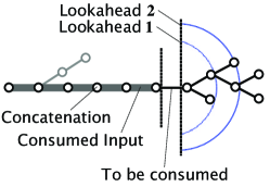
Figure 3. Matching

One can execute an abstract transducer on a rooted and directed graph instead of a particular input word—one word corresponds to a list or a sequence of letters. Each edge of the graph that we match is labeled with a letter. Words are formed by concatenating all letters on the graph edges that get traversed during the matching process, starting from the root node of the graph. Figure 3 provides an intuition of the matching process. In this work, we restrict the graph matching process to disjunctive tree matching, defined by:

Definition 4.9 (Disjunctive Tree Matching).

A tree matching procedure is called to be disjunctive if not several input branches that follow from a particular point on have to satisfy specific criteria. That is, if only one of the input words that follow (on that the lookahead is conducted), must satisfy a given criterion.

To allow for matching based on the full expressiveness of regular tree expressions (several of the input words might have to satisfy a specific criterion), the abstract transducer’s abstract input domain has to be lifted from an abstract word domain to an abstract language domain—see Sect. 3.1. We keep this extension of abstract transducers for future work.

4.4. Epsilon Closure

An established practice (Hopcroft et al., 2003; Sipser, 1997) in automata theory and its application is to use automata with transitions that are annotated with an empty-word symbol $\epsilon$. This was, first and foremost, introduced as a convenience feature to describe automata and its transition relation in a more concise fashion. Abstract transducers allow to annotate transitions with the abstract epsilon word $\mathfrak{v}_{\epsilon}$ to provide similar semantics and convenience:

Definition 4.10 ($\epsilon$-Move).

An $\epsilon$-move (or $\epsilon$-transition) is an automaton transition (or transducer transition) $(q,\mathfrak{v},q^{\prime},{\mathfrak{w}})\in\delta$ that is annotated with the abstract epsilon word $\mathfrak{v}_{\epsilon}$ as its input, that is, $[\![\mathfrak{v}]\!]_{\text{in}}=[\![\mathfrak{v}_{\epsilon}]\!]_{\text{in}}=\{\epsilon\}$.

Some algorithms might not be able to deal with transducers that have $\epsilon$-moves—or they might be more sophisticated in their presence—but only with those transducers from that all $\epsilon$-moves were eliminated. We define abstract transducers without $\epsilon$-moves as:

Definition 4.11 (Input-$\epsilon$-Free).

An abstract transducer is said to be input-$\epsilon$-free if it does not have any transition based on an $\epsilon$-move, that is, $(\cdot,\mathfrak{v}_{\epsilon},\cdot,\cdot)\not\in\delta$, with $[\![\mathfrak{v}_{\epsilon}]\!]_{\text{in}}=\{\epsilon\}$.

The presence of $\epsilon$-moves can lead to loops thereof, which is vital for expressing complex outputs, for example, to describe the control-flow of Turing-complete programs—assuming that each move emits a program operation to conduct as output.

Definition 4.12 ($\epsilon$-Loop).

An $\epsilon$-loop is any sequence of $\epsilon$-moves that starts in a control state $q_{k}$ and could include this control state $q_{k}$ infinitely often in such a sequence. More formally, an $\epsilon$-loop is a sequence $\bar{\tau}=\langle\tau_{1},\ldots,\tau_{n}\rangle\in\Delta^{\infty}$ of $\epsilon$-moves that is well-founded in the transition relation $\delta$ and there exists a transducer transition $\tau_{i}=(q,\cdot,\cdot,\cdot)\in\bar{\tau}$ for which the source state $q$ is precisely the destination state $q^{\prime}$ of a transducer transition $\tau_{j}=(\cdot,\cdot,q^{\prime},\cdot)\in\bar{\tau}$, with $i\leq j$.

From the definition of $\epsilon$-moves follows the definition of the $\epsilon$-closure (Sipser, 1997). Intuitively speaking the $\epsilon$-closure of a control state $q$ is the set of control states that become instantly and simultaneously (parallel) active if state $q$ becomes active.

Definition 4.13 (Epsilon Closure).

The epsilon closure $\mathsf{epsclosure}:Q\rightarrow 2^{Q}$ of a state $q\in Q$ is the set $\mathsf{epsclosure}(q)\subseteq Q$ of states that can get reached transitively from state $q$ by only following $\epsilon$-moves (Sipser, 1997). The bottom state $q_{\bot}$ is added if the epsilon closure includes an $\epsilon$-loop from which no control state is reachable with no $\epsilon$-move leaving.

The transition relation of an abstract transducer can contain sequences $\{(q_{1},\mathfrak{v}_{\epsilon},q_{2},\allowbreak{\mathfrak{w}}_{1}),\allowbreak(q_{2},\mathfrak{v}_{\epsilon},q_{3},{\mathfrak{w}}_{2})\}\subseteq\delta$ of $\epsilon$-moves but not each control state that is reached within such a sequence might have non-$\epsilon$-moves leaving in the transition relation. We therefore introduce the notion of closure termination states:

Definition 4.14 (Closure Termination States).

The closure termination states ${\mathsf{closureterm}}:Q\rightarrow 2^{Q}$ of a given state $q$ are both the states (1) in the epsilon closure $\mathsf{epsclosure}(q)$ from which no $\epsilon$-move leaves and (2) states within the closure that are accepting, that is, ${\mathsf{closureterm}}(q)=\{q^{\prime}\;|\;q^{\prime}\in\mathsf{epsclosure}(q)\land(q^{\prime},\mathfrak{v}_{\epsilon},\cdot,\cdot)\not\in\delta\}\cup(\mathsf{epsclosure}(q)\cap F)$.

Each transducer transition between the control states from an $\epsilon$-closure can be mapped to a set of closure termination states:

Definition 4.15 (Termination State Mapping).

The termination state mapping is a map $\Delta_{\Omega}:\Delta\rightarrow 2^{Q}$ that maps a given transducer transition to the set of closure termination states that are reachable. Given a control state $q\in Q$, the result is the empty set $\emptyset$ if no $\epsilon$-move leaves state $q$; it is the bottom state $q_{\bot}$ if there is not any other termination state.

Since also each transition within an epsilon closure can produce an output, we introduce the notion of concrete language on termination. This notion reflects with which output words the different closure termination states can be reached:

Definition 4.16 (Concrete Language on Termination).

The concrete language on termination $\Omega:Q\times Q\rightarrow 2^{\Theta^{\infty}}$ for a given pair $(q,q_{\Omega})$ describes the concrete output language (a set of concrete words) that can be produced starting in control state $q$ and that terminates with a closure termination state $q_{\Omega}\in{\mathsf{closureterm}}(q)$. More formally, let $\widehat{\tau}=\{\bar{\tau}_{1},\ldots\}\subseteq\Delta^{\infty}$ be the set of all well-founded sequences of transducer transitions between control state $q$ and the termination state $q_{\Omega}$, with $\bar{\tau_{i}}=\langle\tau_{1},\ldots\rangle$ and $\tau_{i}=(q,\mathfrak{v}_{i},q^{\prime},{\mathfrak{w}}_{i})\in\delta$. The concrete output language $[\![\bar{\tau_{i}}]\!]$ of a sequence $\bar{\tau_{i}}$ is the concatenation $[\![{\mathfrak{w}}_{1}]\!]_{\text{out}}\circ\ldots$ of the concretizations of all abstract output words ${\mathfrak{w}}_{i}$ that are emitted along it. That is, the concrete output language $\Omega(q,q_{\Omega})$ is the union $\bigcup_{\bar{\tau_{i}}\in\widehat{\tau}}\;[\![\bar{\tau_{i}}]\!]$.

Definition 4.17 (Concrete Closure Language).

The concrete closure language $\Omega(q)\subseteq{\Theta^{\infty}}$ of a given control state $q$ and its $\epsilon$-closure is the set of concrete output words that is produced while making transitions along the $\epsilon$-moves between states in the closure. More precisely, it is the join of concrete languages on termination, that is, $\Omega(q)=\bigcup\;\{\bar{\sigma}\in\Omega(q,q_{\Omega})\;|\;q_{\Omega}\in{\mathsf{closureterm}}(q)\}$.

In our applications of abstract transducers, we use the (anonymous) states and transitions in the epsilon closure as a tool for expressing relational outputs. Please note, that also $\epsilon$-moves that lead to a dead-end are relevant and must not be eliminated—what is done for some applications (D’Antoni and Veanes, 2017b)—because the output might be relevant for the analysis task, and the soundness of the produced result, for which the transducer is executed.

Figure 4. With $\epsilon$-loop

Example 4.18.

Figure 4 illustrates an example transducer: The $\epsilon$-closure of control state $q_{0}$ is the set $\mathsf{epsclosure}(q_{0})=\{q_{0},q_{1},q_{2},q_{3},q_{4},q_{\bot}\}$, for state $q_{2}$, the closure $\mathsf{epsclosure}(q_{2})=\{q_{2}\}$ does not contain additional states. State $q_{0}$ has the set of closure termination states ${\mathsf{closureterm}}(q_{0})=\{q_{2},q_{\bot}\}$, and state $q_{1}$ has ${\mathsf{closureterm}}(q_{1})=\{q_{\bot}\}$, that is, no other termination state is reachable. The transitions between states $\{q_{1},q_{3},q_{4}\}$ form an $\epsilon$-loop.

Given a control state $q\in Q$, the semantics of $\epsilon$-moves implies that with reaching state $q$, actually all states in $Q_{t}={\mathsf{closureterm}}(q)$ are reached immediately. That is, also all output on the transitions from $q$ to a state in $Q_{t}$ is produced immediately, resulting in—possibly exponentially many and infinitely long—words $\subseteq{\Theta^{\infty}}$ over the output alphabet $\Theta$.

4.5. Output Closure

Previous section describes the epsilon closure of abstract transducers; in contrast to established transducer concepts, we also address $\epsilon$-moves that are annotated with non-empty outputs, and use them as tool to express complex output languages, with possibly exponentially many and infinitely long words, in a convenient fashion. When executing or reducing (minimizing) abstract transducers, means for collecting, aggregating, and possibly abstracting the output on these transitions are needed. Given a control state $q\in Q$, the goal of this summarization process is to provide an abstract output word ${\mathfrak{w}}_{\Omega}\in\mathfrak{W}$ for each of its closure termination states $q_{\Omega}\in{\mathsf{closureterm}}(q)$ that overapproximates the concrete closure language, that is, $\Omega(q,q_{\Omega})\subseteq[\![{\mathfrak{w}}_{\Omega}]\!]_{\text{out}}$—which can lead to a loss of information. The computation of this closure is done in a corresponding operator:

Definition 4.19 (Abstract Output Closure).

The abstract output closure of a given control state $q\in Q$ is a finite overapproximation of the concrete closure language of each of its closure termination states; it is a map of closure termination states of $q$ to abstract output words, which summarizes the corresponding closure output languages: $\mathsf{abstclosure}:(Q\times\mathfrak{W})\rightarrow 2^{Q\rightarrow\mathfrak{W}}$. A call $\mathsf{abstclosure}(q,{\mathfrak{w}}_{0})$, with an initial abstract output word ${\mathfrak{w}}_{0}$, returns a map $\{(q_{t},{\mathfrak{w}}_{t})\;|\;q_{t}\in{\mathsf{closureterm}}(q)\land[\![{\mathfrak{w}}_{t}]\!]_{\text{out}}\subseteq[\![{\mathfrak{w}}_{0}]\!]_{\text{out}}\circ\Omega(q,q_{t})\}$.

We extend the abstract output closure operator $\mathsf{abstclosure}$ to sets:

Definition 4.20 (Abstract Output Closure).

The abstract output closure of a given set of transducer states $\widehat{\mathsf{abstclosure}}:2^{Q\times\mathfrak{W}}\rightarrow 2^{Q\rightarrow\mathfrak{W}}$ is defined as $\widehat{\mathsf{abstclosure}}(S)=\bigsqcup_{\rightarrow}\bigcup\;\{(q_{\Omega},{\mathfrak{w}}_{\Omega})\;|\allowbreak\;\allowbreak(q,{\mathfrak{w}}_{0})\in S\land\allowbreak(q_{\Omega},{\mathfrak{w}}_{\Omega})\in\mathsf{abstclosure}(q,{\mathfrak{w}}_{0})\}$.

Actual implementations of an abstract output closure operator can be provided, for example, based on abstract interpretation, or based on techniques from automata theory. Even transducers can be used (Preda et al., 2016) to compute abstractions of languages, in our case, the concrete output languages that are produced in the $\epsilon$-closure. We give two examples of implementations:

4.5.1. Joining Closure

The first abstract output closure operator $\mathsf{abstclosure}_{\sqcup}$ joins all abstract output words that can be found on transitions in the epsilon closure from control state $q$ that are mapped to the same closure termination state. Let us assume that there is an operation $\textsf{closuretrans}:Q\times Q\rightarrow 2^{\Delta}$ that, given a pair of control states $q,q_{\Omega}\in Q$, returns all transitions from the transition relation $\delta$ that are in the epsilon closure $\mathsf{epsclosure}(q)$ and are mapped to a closure termination state $q_{\Omega}$. Then, we can define the closure operator as follows: $\mathsf{abstclosure}_{\sqcup}(q,{\mathfrak{w}}_{0})=\allowbreak\{(q_{\Omega},{\mathfrak{w}}_{0}\sqcup_{\text{out}}\bigsqcup_{\text{out}}\{{\mathfrak{w}}\;|\allowbreak\;(\cdot,\cdot,\cdot,{\mathfrak{w}})\in\textsf{closuretrans}(q,q_{\Omega})\})\;|\allowbreak\;q_{\Omega}\in{\mathsf{closureterm}}(q)\}$. This operator produces an overapproximation of the concrete output language. The resulting abstraction does neither preserve information on the flow nor is path information kept.

4.5.2. Regular Closure

Another example of an output closure operator is $\mathsf{abstclosure}_{\infty}$. Here, we assume that the abstract output words can be described based on an abstract domain of $\infty$-regular languages (Löding and Tollkötter, 2016), with a corresponding lattice thereof. Rules for transforming automata into regular expressions can be applied (Löding and Tollkötter, 2016): The result for the transducer in Fig. 4 is ${\mathsf{abstclosure}_{\infty}}(q_{0},{\mathfrak{w}}_{0})=\{(q_{2},{\mathfrak{w}}_{0}\circ{\mathfrak{w}}_{b}),(q_{\bot},{\mathfrak{w}}_{0}\circ{\mathfrak{w}}_{a}\circ({\mathfrak{w}}_{c}\circ{\mathfrak{w}}_{f}\circ{\mathfrak{w}}_{d})^{\omega})\}$. This type of output closure is lossless. Nevertheless, not all applications require this level of detail.

4.6. Runs

We now define runs of abstract transducers and illustrate how they are conducted for given inputs. All runs of an abstract transducer start from the initial transducer state:

Definition 4.21 (Abstract Transducer Run).

A run of an abstract transducer on a concrete input word $\bar{\sigma}=\langle\sigma_{1},\allowbreak\ldots,\allowbreak\sigma_{n}\rangle\in\Sigma^{*}$ and a lookahead ${\widehat{\sigma}}\subseteq\Sigma^{*}$ is a sequence of transducer state transitions ${\iota_{0}}\smash{\xrightarrow{\mathfrak{v}_{1}/{\mathfrak{w}}_{1}}}\ldots\smash{\xrightarrow{\mathfrak{v}_{n}/{\mathfrak{w}}_{n}}}\iota_{n}$, also denoted by $\langle{\iota_{0}},\ldots,\iota_{n}\rangle$ in case the actual transducer transitions are irrelevant for the discussion. A run always starts in the initial transducer state ${\iota_{0}}\in J$, is well-founded in the transition relation $\delta$, and all transitions along the input match, that is, the quotienting $(\langle\!\langle\{\langle\sigma_{i},\ldots,\sigma_{n}\rangle\}\circ{\widehat{\sigma}}\rangle\!\rangle_{\text{in}})^{\mathfrak{v}_{i}}\neq{\bot}$ does not result in the abstract bottom word.

Before we continue to define feasible and accepting runs of an abstract transducer, we define the abstract output of a run:

Definition 4.22 (Abstract Run Output).

The abstract output of a run $\iota_{0}\smash{\xrightarrow{\mathfrak{v}_{1}/{\mathfrak{w}}_{1}}}\ldots\smash{\xrightarrow{\mathfrak{v}_{n}/{\mathfrak{w}}_{n}}}\iota_{n}$ is the concatenation of the subsequent abstract output words ${\mathfrak{w}}_{\circ}={\mathfrak{w}}_{0}\circ{\mathfrak{w}}_{1}\circ\ldots\circ{\mathfrak{w}}_{n}$. The abstract output word ${\mathfrak{w}}_{0}$ is one abstract output word from the initial transducer state, that is, there exists a pair $(\cdot,{\mathfrak{w}}_{0})\in{\iota_{0}}$.

The output of a abstract transducer run is essential for the definition of feasible transducer runs:

Definition 4.23 (Feasible Run).

A run is called feasible if and only if its abstract output ${\mathfrak{w}}_{\circ}$ is not the bottom element $\bot$, that is, if and only if $[\![{\mathfrak{w}}_{\circ}]\!]_{\text{out}}\neq\emptyset$. The set of all concrete inputs (with lookaheads) that result in a feasible run on an abstract transducer $\mathsf{T}$ defines the function $\textsf{feasible}_{\mathsf{T}}:\Sigma^{*}\times 2^{\Sigma^{*}}\rightarrow\mathbb{B}$.

Abstract transducers can also operate as acceptors and define a set of inputs to be accepted. We first define the notion of an accepting run and define the accepted input language later:

Definition 4.24 (Accepting Run).

A run $\langle\iota_{0},\ldots,\iota_{n}\rangle$ is called to be accepting if it is feasible and its last transducer state contains an accepting (final) control state, that is, if and only if $(q_{n},{\mathfrak{w}}_{n})\in\iota_{n}$, with $q_{n}\in F$ and ${\mathfrak{w}}_{n}\neq\bot$.

In general, an abstract transducer is a nondeterministic automaton, nevertheless it can be deterministic if it satisfies following criterion:

Definition 4.25 (Deterministic Abstract Transducer).

We call an abstract transducer deterministic if and only if it does not allow a run $\bar{\iota}=\langle\iota_{0},\ldots\iota_{n}\rangle$ with a transducer state $\iota_{i}\in\bar{\iota}$ that consists of more than one element, that is, $\forall\iota_{i}\in\bar{\iota}:|\iota_{i}|\leq 1$.

We now continue with an operational perspective on the runs of an abstract transducer. Given a concrete input word ${\bar{\sigma}}\in\Sigma^{*}$ based on the concrete input alphabet $\Sigma$ and a set ${\widehat{\sigma}}\subseteq\Sigma^{*}$ of words that can follow to this word (used for the lookahead), which output does the transducer produce and does processing the word terminate in an accepting control state? Since a concrete input word can be represented as an abstract word, and we consider this the more general case, we describe runs based on abstract input words: A given concrete input word $\bar{\sigma}\in\Sigma^{*}$ can be transformed to an abstract input word by applying the abstraction operator such that we end up in an abstract word $\mathfrak{v}=\langle\!\langle\{\bar{\sigma}\}\rangle\!\rangle_{\text{in}}$, with $[\![\mathfrak{v}]\!]_{\text{in}}=\{\bar{\sigma}\}$.

Definition 4.26 (Run).

The function $\mathsf{run}_{\mathsf{T}}:Q\times\mathfrak{W}\times\mathfrak{I}\times\mathfrak{I}\rightarrow 2^{Q\rightarrow\mathfrak{W}}$ conducts a run starting from a control state $q\in Q$, an initial abstract output word ${\mathfrak{w}}\in\mathfrak{W}$, an abstract input word $\mathfrak{v}\in\mathfrak{I}$, with $\mathfrak{v}\neq\bot$, and an abstract word $\mathfrak{v}_{\ell}\in\mathfrak{I}$ that describes the lookahead that must be satisfied:

$$\mathsf{run}_{\mathsf{T}}(q,{\mathfrak{w}},\mathfrak{v},\mathfrak{v}_{\ell})=\begin{dcases*}\{\;(q,{\mathfrak{w}})\;\}&\text{if $\mathfrak{v}=\mathfrak{v}_{\epsilon}$}\\ \bigsqcup_{\rightarrow}\;\bigcup\;\{\;\mathsf{run}_{\mathsf{T}}({q^{\prime\prime},{\mathfrak{w}}\circ{\mathfrak{w}}^{\prime\prime},\textsf{tail}(\mathfrak{v}),\mathfrak{v}_{\ell}})\;|\;\\ \quad(q,\mathfrak{v}_{\tau},q^{\prime},{\mathfrak{w}}^{\prime})\in\delta\\ \quad\land\;(q^{\prime\prime},{\mathfrak{w}}^{\prime\prime})\in\mathsf{abstclosure}(q^{\prime},{\mathfrak{w}}^{\prime})\\ \quad\land\;(\mathfrak{v}\circ\mathfrak{v}_{\ell})^{\mathfrak{v}_{\tau}}\neq\bot\\ \quad\land\;(\textsf{head}(\mathfrak{v}))^{\textsf{head}(\mathfrak{v}_{\tau})}\neq\bot\;\}&\text{otherwise}\\ \end{dcases*}$$

The function $\mathsf{run}$ terminates its recursion if the abstract input word is the bottom element. The recursive call to $\mathsf{run}$ is done for the tail of the abstract input word—which ensures termination—in case a transition that leaves the given control state $q$ matched the input.

We extend this function to $\widehat{\mathsf{run}}_{\mathsf{T}}:2^{Q\rightarrow\mathfrak{W}}\times\mathfrak{I}\times\mathfrak{I}\rightarrow 2^{Q\rightarrow\mathfrak{W}}$, which starts from a transducer state, and we define it as follows:

$$\widehat{\mathsf{run}}_{\mathsf{T}}(\iota,\mathfrak{v},\mathfrak{v}_{\ell})=\bigsqcup_{\rightarrow}\bigcup_{\quad(q,{\mathfrak{w}})\in\iota}\mathsf{run}_{\mathsf{T}}(q,{\mathfrak{w}},\mathfrak{v},\mathfrak{v}_{\ell})$$

The transducer state to start from is omitted if it is the abstract transducer‘s initial transducer state ${\iota_{0}}$, that is, $\widehat{\mathsf{run}}_{\mathsf{T}}(\mathfrak{v},\mathfrak{v}_{\ell})=\widehat{\mathsf{run}}_{\mathsf{T}}({\iota_{0}},\mathfrak{v},\mathfrak{v}_{\ell})$. Given a concrete input word $\bar{\sigma}\in\Sigma^{*}$ and a corresponding set of concrete words $\widehat{\sigma}\subseteq\Sigma^{*}$ for the lookahead, we write $\widehat{\mathsf{run}}_{\mathsf{T}}(\bar{\sigma},\widehat{\sigma})$ as an abbreviation for $\widehat{\mathsf{run}}_{\mathsf{T}}({\iota_{0}},\bar{\sigma},\widehat{\sigma})$, which is as an abbreviation for $\widehat{\mathsf{run}}_{\mathsf{T}}({\iota_{0}},\langle\!\langle\{\bar{\sigma}\}\rangle\!\rangle_{\text{in}},\langle\!\langle\widehat{\sigma}\rangle\!\rangle_{\text{in}})$.

4.7. Languages and Transductions

Contrary to other types of finite state transducers (D’Antoni and Veanes, 2015) our abstract transducers distinguish between two type of input languages: the intermediate input language and the accepted input language.

Definition 4.27 (Intermediate Input Language).

The intermediate input language $\mathcal{L}_{\textit{in}}(\mathsf{T})\subseteq\Sigma^{*}\times 2^{\Sigma^{*}}$ of an abstract transducer $\mathsf{T}$ is the set of concrete input words for that the transducer can conduct feasible runs starting from the initial transducer state ${\iota_{0}}$:

$$\mathcal{L}_{\textit{in}}(\mathsf{T})=\{\;({\bar{\sigma}},{\widehat{\sigma}})\;|\;\textsf{feasible}_{\mathsf{T}}({\bar{\sigma}},{\widehat{\sigma}})\land{\bar{\sigma}}\in\Sigma^{*}\land{\widehat{\sigma}}\subseteq\Sigma^{*}\;\}.$$

It follows that each prefix $\bar{\sigma}_{p}\preceq\bar{\sigma}$ of each word $\bar{\sigma}\in\mathcal{L}_{\textit{in}}(\mathsf{T})$ is also element of the intermediate input language, that is, $\bar{\sigma}_{p}\in\mathcal{L}_{\textit{in}}(\mathsf{T})$.

The accepted input language reflects the established notion of input language, which is based on the set of words that can reach a final control state:

Definition 4.28 (Accepted Input Language).

The accepted input language $\mathcal{L}_{\textit{acc}}\subseteq\mathcal{L}_{\textit{in}}$ is the subset of the intermediate input language for which an accepting control state $q\in F$ is reached:

$$\mathcal{L}_{\textit{acc}}(\mathsf{T})=\{\;(\bar{\sigma},\widehat{\sigma})\in\mathcal{L}_{\textit{in}}(\mathsf{T})\;|\;(q,\cdot)\in\widehat{\mathsf{run}}_{\mathsf{T}}(\bar{\sigma},\widehat{\sigma})\land q\in F\;\}.$$

Beside the accepted input language, another characteristic of an abstract transducer is its set of transductions and its set of accepting transductions:

Definition 4.29 (Transductions).

The set of transductions $\mathcal{T}(\mathsf{T})\subseteq\Sigma^{*}\times 2^{\Sigma^{*}}\times 2^{\Theta^{\infty}}$ of an abstract transducer $\mathsf{T}$ characterizes both its concrete input language and the outputs that are produced for them. One element $({\bar{\sigma}},\bar{\Sigma}_{\ell},\bar{\Theta})\in\mathcal{T}(\mathsf{T})$ from this set is a tuple that consists of a word prefix ${\bar{\sigma}}$ that is consumed by a run of the transducer, a set of concrete words $\bar{\Theta}\subseteq\Sigma^{*}$ to conduct the lookahead on and that remains to be consumed by the next transitions of the transducer, and the set of concrete output words $\bar{\Theta}\subseteq\Theta^{\infty}$ that are emitted with the consumption of word ${\bar{\sigma}}$—see the definition of $\widehat{\mathsf{run}}_{\mathsf{T}}$ for more details:

$$\mathcal{T}(\mathsf{T})=\bigcup\;\{\; (\bar{\sigma},\widehat{\sigma},[\![{\mathfrak{w}}]\!]_{\text{out}})\;|\;(\bar{\sigma},\widehat{\sigma})\in\mathcal{L}_{\textit{in}}(\mathsf{T})\;$$

$$\land(q,{\mathfrak{w}})\in\widehat{\mathsf{run}}_{\mathsf{T}}(\bar{\sigma},\widehat{\sigma})\;\}.$$

Definition 4.30 (Accepting Transductions).

The set of accepting transductions $\mathcal{T}_{\text{acc}}(\mathsf{T})\subseteq\mathcal{T}(\mathsf{T})$ is the subset of the transductions of a given abstract transducer $\mathsf{T}$ that are produced by accepting runs:

$$\mathcal{T}(\mathsf{T})=\bigcup\;\{\; (\bar{\sigma},\widehat{\sigma},[\![{\mathfrak{w}}]\!]_{\text{out}})\;|\;(\bar{\sigma},\widehat{\sigma})\in\mathcal{L}_{\textit{in}}(\mathsf{T})$$

$$\land(q,{\mathfrak{w}})\in\widehat{\mathsf{run}}_{\mathsf{T}}(\bar{\sigma},\widehat{\sigma})$$

$$\land q\in F\;\}.$$

The number of accepting transductions is greater or equal than the number of accepted input words, that is, $|\mathcal{L}_{\textit{acc}}(\mathsf{T})|\leq|\mathcal{T}_{\text{acc}}(\mathsf{T})|$, because there can be independent concrete output languages for one concrete input $(\bar{\sigma},\widehat{\sigma})\in\Sigma^{*}\times 2^{\Sigma^{*}}$.

In combination, the set of transductions and the set of accepted transductions determine if two abstract transducers are equivalent to each other:

Definition 4.31 (Equivalence).

Two abstract transducers $\mathsf{T}_{1},\mathsf{T}_{2}\in\mathbb{T}$ are called equivalent $\mathsf{T}_{1}\equiv\mathsf{T}_{2}$ to each other if and only if both have the same set of transductions and the same set of accepting transductions, that is, if and only if $\mathcal{T}(\mathsf{T}_{1})=\mathcal{T}(\mathsf{T}_{2})$ and $\mathcal{T}_{\text{acc}}(\mathsf{T}_{1})=\mathcal{T}_{\text{acc}}(\mathsf{T}_{2})$.

Based on the notion of equality, we can define different operations, for example, reduction or $\epsilon$-elimination. We start by defining a more fundamental one: The union of two abstract transducers. The union is constructed similar to the union of $\epsilon$-NFAs, with the exception that no $\epsilon$-moves are added; we take advantage of the fact that the initial transducer state is a set:

Definition 4.32 (Union).

Given two abstract transducers $\mathsf{T}_{1},\mathsf{T}_{2}\in\mathbb{T}_{{\overline{D}_{\text{in}}}\times{\overline{D}_{\text{out}}}}$ that both have the same abstract input domain ${\overline{D}_{\text{in}}}$ and the same abstract output domain ${\overline{D}_{\text{out}}}$, such that $\mathsf{T}_{1}=(Q_{1},{\overline{D}_{\text{in}}},{\overline{D}_{\text{out}}},{\iota_{0}}_{1},F_{1},\delta_{1})$ and $\mathsf{T}_{2}=(Q_{2},{\overline{D}_{\text{in}}},{\overline{D}_{\text{out}}},{\iota_{0}}_{2},F_{2},\delta_{2})$. The union $\cup:\mathbb{T}\times\mathbb{T}\rightarrow\mathbb{T}$ of two abstract transducers results in a new abstract transducer $\mathsf{T}_{\cup}=\mathsf{T}_{1}\cup\mathsf{T}_{2}$ that maintains exactly both the union of the set of transductions and the set of accepting transductions, that is, $\mathcal{T}(\mathsf{T}_{\cup})=\mathcal{T}(\mathsf{T}_{1})\cup\mathcal{T}(\mathsf{T}_{2})$ and $\mathcal{T}_{\text{acc}}(\mathsf{T}_{\cup})=\mathcal{T}_{\text{acc}}(\mathsf{T}_{1})\cup\mathcal{T}_{\text{acc}}(\mathsf{T}_{2})$. We define the union as $\mathsf{T}_{\cup}=\cup(\mathsf{T}_{1},\mathsf{T}_{2})=(Q_{1}\cup Q_{2},{\overline{D}_{\text{in}}},{\overline{D}_{\text{out}}},{\iota_{0}}_{1}\cup{\iota_{0}}_{2},F_{1}\cup F_{2},\delta_{1}\cup\delta_{2})$.

4.8. Elimination of $\epsilon$-Moves

Since $\epsilon$-moves are considered to be a convenience feature, eliminating them without losing any output must be possible—that is, without altering the semantics of the transducer. The $\epsilon$-closure can allow sequences of state transitions of infinite length, that is, a means to encode this infinite information into one (finite) output symbol is needed. An algorithm for computing abstract output closures provides such a means.

For the design of an $\epsilon$-elimination algorithm, it is important to note that all states in the $\epsilon$-closure of a control state become active when it is entered. This implies that then also the output that is produced along with these $\epsilon$-moves must be emitted: Existing algorithms for $\epsilon$-elimination are not applicable to abstract transducers. An algorithm for eliminating $\epsilon$-moves from an abstract transducer $\mathsf{T}_{\epsilon}$ must ensure that the resulting transducer $\mathsf{T}$ is equivalent $\mathsf{T}_{\epsilon}\equiv\mathsf{T}$. Please note that stuttering transitions must be made explicit and must be considered to allow a sound elimination of $\epsilon$-moves.

Algorithm 1 $\textsf{elim}{}(\mathsf{T}_{\epsilon})$

0:  Abstract transducer $\mathsf{T}_{\epsilon}=(Q,{\overline{D}_{\text{in}}},{\overline{D}_{\text{out}}},{\iota_{0}},F,\delta)\in\mathbb{T}$

0:  Abstract transducer $\mathsf{T}\in\mathbb{T}$, with $\mathsf{T}_{\epsilon}\equiv\mathsf{T}$
// Sentinel transitions for the initial transducer state, with $\mathfrak{v}_{\epsilon}\not\equiv\mathfrak{v}_{\text{start}}$

1:  $\delta_{\epsilon}=\delta\cup\{\;(q_{s},\mathfrak{v}_{\text{start}},q,{\mathfrak{w}})\;|\;(q,{\mathfrak{w}})\in{\iota_{0}}\;\}$
// Shortcut $\epsilon$-moves to their termination states

2:  $\delta^{\prime}=\{\;(q,\mathfrak{v},q^{\prime\prime},{\mathfrak{w}}^{\prime\prime})\;|\;\tau=(q,\mathfrak{v},q^{\prime},{\mathfrak{w}})\in\delta_{\epsilon}\newline \quad\quad\quad\land\mathfrak{v}\neq\mathfrak{v}_{\epsilon}\land(q^{\prime\prime},{\mathfrak{w}}^{\prime\prime})\in\mathsf{abstclosure}(\{(q^{\prime},{\mathfrak{w}})\})\;\}$
// Reconstruct a new initial transducer state

3:  ${\iota_{0}}^{\prime}=\{\;(q,{\mathfrak{w}})\;|\;(\cdot,\mathfrak{v},q,{\mathfrak{w}})\in\delta\land\mathfrak{v}=\mathfrak{v}_{\text{start}}\;\}$
// Reassemble the components to a new abstract transducer

4:  return $(Q,{\overline{D}_{\text{in}}},{\overline{D}_{\text{out}}},{\iota_{0}}^{\prime},F,\delta^{\prime})$

Algorithm 1 is our approach for eliminating $\epsilon$-moves from an abstract transducer. The algorithm constructs a new transition relation, from which all $\epsilon$-moves are removed by adding shortcuts to the closure termination states and concatenating the corresponding closure output language.

Proposition 4.33.

Given an abstract transducer $\mathsf{T}_{\epsilon}$, all its $\epsilon$-moves can be eliminated without affecting its semantics, that is, without affecting either the set of transductions or the set of accepting transductions. The abstract transducer $\mathsf{T}_{\epsilon}$ can be transformed into an input-$\epsilon$-free transducer $\mathsf{T}$, with $\mathsf{T}_{\epsilon}\equiv\mathsf{T}$.

Proof.

We prove the proposition by providing an algorithm that conducts this transformation while maintaining the set of transductions and the set of accepted transductions: Given an abstract transducer $\mathsf{T}_{\epsilon}$ that has $\epsilon$-moves, Algorithm 1—which we implicitly parameterize with the output closure operator $\mathsf{abstclosure}_{\infty}$—produces an abstract transducer $\mathsf{T}$ that is input-$\epsilon$-free and satisfies $\mathcal{T}(\mathsf{T}_{\epsilon})=\mathcal{T}(\mathsf{T})$ and $\mathcal{T}_{\text{acc}}(\mathsf{T}_{\epsilon})=\mathcal{T}_{\text{acc}}(\mathsf{T})$. (1) The transition relation $\delta^{\prime}$, and with it the resulting transducer $\mathsf{T}$, is input-$\epsilon$-free because only non-$\epsilon$-moves are added to the transition relation. (2) The set of closure termination states, for which $\mathsf{abstclosure}_{\infty}$ provides a pairing with the corresponding output closure language, contains all accepting states (Definition 4.14), that is, all moves to accepting states are maintained, and with it the set of accepting transductions. (3) The set of transductions is maintained: The output from the epsilon closures, that is, the closure termination languages, are concatenated to the transitions to the closure termination states. ∎

Example 4.34.

Given the transducer in Fig. 4, Algorithm 1 proceeds as follows: First, we extend the transition relation with sentinels and get $\delta_{\epsilon}=\{(q_{0},\mathfrak{v}_{\epsilon},q_{1},{\mathfrak{w}}_{a}),\allowbreak(q_{1},\mathfrak{v}_{\epsilon},q_{3},{\mathfrak{w}}_{c}),\allowbreak(q_{3},\mathfrak{v}_{\epsilon},q_{4},{\mathfrak{w}}_{f}),\allowbreak(q_{4},\mathfrak{v}_{\epsilon},q_{1},{\mathfrak{w}}_{d}),\allowbreak(q_{0},\mathfrak{v}_{\epsilon},q_{2},{\mathfrak{w}}_{b}),\allowbreak(q_{2},\mathfrak{v}_{\epsilon},q_{5},{\mathfrak{w}}_{e}),\allowbreak(q_{s},\mathfrak{v}_{\text{start}},\allowbreak q_{0},\mathfrak{v}_{\epsilon})\}$. In the next step, $\epsilon$-moves are left out by adding transitions to the closure termination states and concatenating the corresponding closure output languages; the result is a new transition relation $\delta^{\prime}=\{(q_{s},\mathfrak{v}_{\text{start}},q_{\bot},{\mathfrak{w}}_{\ast}),\allowbreak(q_{s},\mathfrak{v}_{\text{start}},q_{2},{\mathfrak{w}}_{b}),\allowbreak(q_{2},\mathfrak{v}_{1},q_{5},{\mathfrak{w}}_{e})\}$, with ${\mathfrak{w}}_{\ast}={\mathfrak{w}}_{a}\circ({\mathfrak{w}}_{c}\circ{\mathfrak{w}}_{f}\circ{\mathfrak{w}}_{d})^{\omega}$. Then, the initial transducer state is re-constructed from the relation $\delta^{\prime}$ and we get ${\iota_{0}}^{\prime}=\{(q_{\bot},{\mathfrak{w}}_{\ast}),(q_{2},{\mathfrak{w}}_{b})\}$. Finally, the transducer is re-assembled and we get the transducer shown in Fig. 3.

4.9. Determinization

A typical operation when dealing with finite state machines is the transformation of a nondeterministic automaton into a deterministic one. This is not possible for abstract transducers in general: The control-flow structure of the state-transitions within the $\epsilon$-closure describes different information flows—that is, sets of output words that reach different closure termination states—as its semantics, which is not the case for classical automata and transducers. For example, a state-space splitting might be intended based on the information of the emitted output—different outputs for the same input that lead to different control states. That is, different closure termination states, which can be accepting states, can have associated different closure termination languages; this separation must be maintained—which is also reflected in our definition of transducer equivalence.

Proposition 4.35.

Not every nondeterministic abstract transducer $\mathsf{T}$ can be transformed into an equivalent deterministic transducer $\mathsf{T}_{d}$, with $\mathsf{T}\equiv\mathsf{T}_{d}$.

Proof.

We proof the proposition by counterexample—assuming that all abstract transducers can be determinized. Given an abstract transducer $\mathsf{T}$ with the set of initial transducer states ${\iota_{0}}=\{(q_{1},{\mathfrak{w}}_{1}),(q_{2},{\mathfrak{w}}_{2})\}$ and the relation $\delta=\{(q_{1},\mathfrak{v}_{1},q_{3},{\mathfrak{w}}_{3}),(q_{2},\mathfrak{v}_{2},q_{4},{\mathfrak{w}}_{4})\}$, with $\langle a\rangle\in[\![\mathfrak{v}_{1}]\!]_{\text{in}}$ and $\langle b\rangle\in[\![\mathfrak{v}_{2}]\!]_{\text{in}}$, it has the set of transductions $\mathcal{T}(\mathsf{T})=\{(\epsilon,\{\epsilon\},[\![{\mathfrak{w}}_{1}]\!]_{\text{out}}),\allowbreak(\epsilon,\{\epsilon\},[\![{\mathfrak{w}}_{2}]\!]_{\text{out}}),\allowbreak(\langle a\rangle,\{\epsilon\},[\![{\mathfrak{w}}_{1}\circ{\mathfrak{w}}_{3}]\!]_{\text{out}}),(\langle b\rangle,\{\epsilon\},[\![{\mathfrak{w}}_{2}\circ{\mathfrak{w}}_{4}]\!]_{\text{out}})\}$. A determinized version would have an initial transducer state with only one element, that is, the initial transducer state can be either ${\iota_{0}}_{1}=\{(q_{0},{\mathfrak{w}}_{1}\sqcup{\mathfrak{w}}_{2})\}$ of a transducer $\mathsf{T}_{1}$ or ${\iota_{0}}_{2}=\{(q_{0},\epsilon)\}$ of a transducer $\mathsf{T}_{2}$. Both are wrong since transducer $\mathsf{T}$ intended an initial state space splitting with different output languages. Transducer $\mathsf{T}_{2}$ does not have the transduction $(\epsilon,\{\epsilon\},[\![{\mathfrak{w}}_{1}\sqcup{\mathfrak{w}}_{2}]\!]_{\text{out}})\in\mathcal{T}(\mathsf{T}_{2})$. The transductions of $\mathsf{T}_{1}$ are not equal to those of $\mathsf{T}$, since $\mathcal{T}(\mathsf{T}_{1})=\{(\epsilon,\{\epsilon\},[\![{\mathfrak{w}}_{1}\sqcup{\mathfrak{w}}_{2}]\!]_{\text{out}}),(\langle a\rangle,\{\epsilon\},[\![({\mathfrak{w}}_{1}\sqcup{\mathfrak{w}}_{2})\circ{\mathfrak{w}}_{3}]\!]_{\text{out}}),(\langle b\rangle,\{\epsilon\},[\![({\mathfrak{w}}_{1}\sqcup{\mathfrak{w}}_{2})\circ{\mathfrak{w}}_{4}]\!]_{\text{out}})\}\neq\mathcal{T}(\mathsf{T})$. ∎

Proposition 4.36.

An abstract transducer needs a set of initial transducer states to allow for an elimination of $\epsilon$-moves. That is, a set of initial transducer states with $|{\iota_{0}}|=1$ is not sufficient for all $\epsilon$-input-free transducers while maintaining their semantics.

Proof.

Implication of the proof for proposition 4.35. ∎

5. Transducer Abstraction

Abstracting (widening) an abstract transducer is a means to provide its output for a larger set of input words, that is, a mechanism to increase sharing and with it the potential of reuse. That is, we explicitly rely on the fact that abstracting an automaton can widen its input language, and introduces non-determinism (Avni and Kupferman, 2013). We discuss different types of abstractions that are relevant for this work—Fig. 5 provides examples for abstractions. Approaches for abstracting classical automata and symbolic automata have been presented in the past (Bultan et al., 2017; Preda et al., 2015), which can also be adopted for abstract transducers.

(a)

(b)

(c)

(d)

Figure 5. Examples for different types of abstractions. Abstractions are applied step-wise from left to right: (a) we start with the unabstracted transducer, (b) we conduct a state abstraction by merging states $q_{0}$ and $q_{1}$, (c) we abstract the input alphabet, (d) we abstract the output alphabet.

Given an abstract transducer $\mathsf{T}$, the abstraction operator $\langle\!\langle\cdot\rangle\!\rangle^{\pi}:\mathbb{T}\rightarrow\mathbb{T}$ with widening—with the abstraction precision $\pi$ as an implicit parameter that determines the level of abstraction to achieve—has to guarantee that the resulting abstraction overapproximates both the set of transductions and the set of accepting transductions:

Definition 5.1 (Overapproximation).

An abstract transducer $\mathsf{T}_{1}$ overapproximates another abstract transducer $\mathsf{T}_{2}$, which we denote by $\mathsf{T}_{2}\models\mathsf{T}_{1}$, if and only if $\mathsf{T}_{1}$ overapproximates both the set of transductions and the set of accepting transductions of transducer $\mathsf{T}_{2}$, that is, $\mathsf{T}_{2}\models\mathsf{T}_{1}$ if and only if $\forall(\bar{\sigma}_{2},\widehat{\sigma}_{2},\widehat{\theta}_{2})\in\mathcal{T}_{\text{acc}}(\mathsf{T}_{2}):\,\exists(\bar{\sigma}_{1},\widehat{\sigma}_{1},\widehat{\theta}_{1})\in\mathcal{T}_{\text{acc}}(\mathsf{T}_{1}):\,\bar{\sigma}_{1}=\bar{\sigma}_{2}\land\widehat{\sigma}_{1}=\widehat{\sigma}_{2}\land\widehat{\theta}_{2}\subseteq_{C}\widehat{\theta}_{1}$ and $\forall(\bar{\sigma}_{2},\widehat{\sigma}_{2},\widehat{\theta}_{2})\in\mathcal{T}(\mathsf{T}_{2}):\,\exists(\bar{\sigma}_{1},\widehat{\sigma}_{1},\widehat{\theta}_{1})\in\mathcal{T}(\mathsf{T}_{1}):\,\bar{\sigma}_{1}=\bar{\sigma}_{2}\land\widehat{\sigma}_{1}=\widehat{\sigma}_{2}\land\widehat{\theta}_{2}\subseteq_{C}\widehat{\theta}_{1}$. The relation $\subseteq_{C}$ denotes the inclusion relation of the concrete language lattice of the output language domain.

5.1. State Abstraction

The classical approach to abstract an automaton is state abstraction, that is, to merge several control states into one (Pinchinat and Marchand, 2000). Please note that this approach can also be used for abstracting output closures, which is the case if control states within an $\epsilon$-closure are merged:

Definition 5.2 (Control State Merge).

A state merge for a given abstract transducer $\mathsf{T}$ is conducted by merging a set of its control states $Q_{m}\subseteq Q$ into into one new state $q_{m}$, and results in a new abstract transducer $\mathsf{T}_{m}$. We denote this process by the operator $\textsf{qmerge}:\mathbb{T}\times 2^{Q}\rightarrow\mathbb{T}$, that is, $\mathsf{T}_{m}=\textsf{qmerge}(\mathsf{T},Q_{m})$. The actual definition of operator qmerge is given by Algorithm 2.

Algorithm 2 $\textsf{qmerge}{}(\mathsf{T},Q_{m})$

0:  Abstract transducer $\mathsf{T}=(Q,{\overline{D}_{\text{in}}},{\overline{D}_{\text{out}}},{\iota_{0}},F,\delta)$,       set $Q_{m}$ of states to merge

0:  Abstract transducer $\mathsf{T}^{\prime}$, with $\mathsf{T}\models\mathsf{T}^{\prime}$

0:  Control state $q_{m}$ that is not in the set $Q$ of transducer $\mathsf{T}$
// Define the abstraction $\alpha$

1:  $\alpha=\{\;(q,q^{\prime})\;|\;q\in Q\land q^{\prime}=q_{m}\,\text{if}\,q\in Q_{m}\,\text{else}\,q^{\prime}=q\;\}$
// New set of control states

2:  $Q^{\prime}=(Q\setminus Q_{m})\cup\{q_{m}\}$
// New set of accepting states

3:  $F^{\prime}=\{\;\alpha(q)\;|\;q\in F\;\}$
// New initial transducer state

4:  ${\iota_{0}}^{\prime}=\bigsqcup_{\rightarrow}\{\;(\alpha(q),M)\;|\;(q,M)\in{\iota_{0}}\;\}$
// New transition relation

5:  $\delta^{\prime}=\{\;(\alpha(q),\mathfrak{v},\alpha(q^{\prime}),{\mathfrak{w}})\;|\;(q,\mathfrak{v},q^{\prime},{\mathfrak{w}})\in\delta\;\}$
// Compose the resulting transducer

6:  return $(Q^{\prime},{\overline{D}_{\text{in}}},{\overline{D}_{\text{out}}},{\iota_{0}}^{\prime},F^{\prime},\delta^{\prime})$

Proposition 5.3.

Given an abstract transducer $\mathsf{T}$, a transformation $\mathsf{T}^{\prime}=\textsf{qmerge}(\mathsf{T},Q_{m})$ results in a new abstract transducer $\mathsf{T}^{\prime}$, with $\mathsf{T}\models\mathsf{T}^{\prime}$, that is, transducer $\mathsf{T}^{\prime}$ overapproximates transducer $\mathsf{T}$.

Proof.

We have to show that (1) each input $({\bar{\sigma}},{\widehat{\sigma}})\in\Sigma^{*}\times 2^{\Sigma^{*}}$ that leads to a feasible run $\iota=\widehat{\mathsf{run}}_{\mathsf{T}}({\bar{\sigma}},{\widehat{\sigma}})$ on $\mathsf{T}$ also leads to a feasible run $\iota^{\prime}=\widehat{\mathsf{run}}_{\mathsf{T}^{\prime}}({\bar{\sigma}},{\widehat{\sigma}})$ on transducer $\mathsf{T}^{\prime}$, and for each element $(q,{\mathfrak{w}})\in\iota$ there exists an element $(q^{\prime},{\mathfrak{w}}^{\prime})\in\iota^{\prime}$, with $[\![{\mathfrak{w}}]\!]\subseteq[\![{\mathfrak{w}}^{\prime}]\!]$. Furthermore, we have to show that (2) each input that leads to an accepting run on transducer $\mathsf{T}$ also lead to an accepting run on transducer $\mathsf{T}^{\prime}$. Given a run $\bar{\iota}=\langle{\iota_{0}},\ldots,\iota_{n}\rangle$ that is feasible on transducer $\mathsf{T}$ for a given input $({\bar{\sigma}},{\widehat{\sigma}})\in\Sigma^{*}\times 2^{\Sigma^{*}}$. The same input will also produce a feasible run $\bar{\iota}^{\prime}=\langle{\iota_{0}}^{\prime},\ldots,\iota_{n}^{\prime}\rangle$ on transducer $\mathsf{T}^{\prime}$. For each $\iota_{i}\in\bar{\iota}$ with $(q_{1},\cdot)\in\iota_{i}$ or $(q_{2},\cdot)\in\iota_{i}$, the corresponding transducer state $\iota_{i}^{\prime}\in\bar{\iota}^{\prime}$ will contain the merged control state $q_{m}$ with a corresponding abstract output word, that is, $(q_{m},{\mathfrak{w}})\in\iota_{i}^{\prime}$. The definition of qmerge ensures that all transitions from either control state $q_{1}$ or $q_{2}$ are also possible from control state $q_{m}$: All transitions in $\delta$ from or to a control state in $Q_{m}$ are replaced by corresponding transitions from or to control state $q_{m}$. In case a control state to merge is included in the initial transducer state ${\iota_{0}}$, it is replaced by control state $q_{m}$ in the initial transducer state ${\iota_{0}}^{\prime}$ of transducer $\mathsf{T}^{\prime}$. The non-deterministic nature of abstract transducers ensures that all transitions that match will also be taken: One control state can have a set of successor states for a given input. The transformation of the set of accepting control states $F$ to the set $F^{\prime}$ ensures that if one of the states to merge was an accepting state, also state $q_{m}$ will become an accepting state; states in $F$ that are not included in $Q_{m}$ stay accepting states in $F^{\prime}$. That is, all transitions—and runs on them—that were possible from or to control states in the set $Q_{m}$ are still possible (lead feasible or accepting runs) in the new abstract transducer $\mathsf{T}^{\prime}$, but now start or end in control state $q_{m}$. ∎

Please note that abstracting abstract transducers by merging control states does neither affect the number of transitions nor their labeling—both the input symbols and the output symbols on transitions stay the same, but output languages of epsilon closures can change.

Definition 5.4 (State Abstraction).

The state abstraction $\langle\!\langle\mathsf{T}\rangle\!\rangle_{Q}^{\pi}$ of an abstract transducer $\mathsf{T}$ results in a new abstract transducer $\mathsf{T}^{\prime}$ that is computed based on an abstraction precision $\pi$, with $\mathsf{T}\models\mathsf{T}^{\prime}$. The abstraction precision determines which states to keep separated and which to combine into one state—which represents the corresponding equivalence class. The abstraction precision $\pi=\langle Q_{1},\ldots,Q_{n}\rangle$ defines a list of disjoint sets of control states that should be combined. A state abstraction is conducted as follows:

$$\langle\!\langle\mathsf{T}\rangle\!\rangle_{Q}^{\pi}=\begin{dcases*}\textsf{qmerge}(\mathsf{T},Q_{1})&\text{if} $\pi=\langle Q_{1}\rangle$\\ \textsf{qmerge}(\langle\!\langle\mathsf{T}\rangle\!\rangle_{Q}^{\langle Q_{2},\ldots,Q_{n}\rangle},Q_{1})&\text{if} $|\pi|>1$ \text{and} $\pi=\langle Q_{1},Q_{2},\ldots\rangle$\\ \end{dcases*}$$

5.2. Input Alphabet Abstraction

An abstraction approach that influences the abstract input words of the transitions is input alphabet abstraction, which is the process of changing the abstract input word $\mathfrak{v}$ of a transducer transition $\tau=(q,\mathfrak{v},q^{\prime},{\mathfrak{w}})\in\delta$ to an new abstract input word $\mathfrak{v}^{\prime}$, with $[\![\mathfrak{v}]\!]_{\text{in}}\subseteq[\![\mathfrak{v}^{\prime}]\!]_{\text{in}}$:

Definition 5.5 (Input Alphabet Abstraction).

An input alphabet abstraction $\langle\!\langle\mathsf{T}\rangle\!\rangle_{I}^{\pi}$ of an abstract transducer $\mathsf{T}$ results in a new abstract transducer were some of the abstract input words of its control transitions were widened based on the given abstraction precision $\pi\in\Pi_{I}$. The abstraction precision $\pi$ for input alphabet abstraction maps an abstraction precision $\pi_{\text{in}}$ that is applicable to the abstract input domain to each of the transducer’s control transitions, that is, it is a left-total function $\pi:\Delta\rightarrow\Pi_{\text{in}}$. The result is an abstract transducer with a widened transition relation:

$$\delta^{\prime}=\{\;(q,\langle\!\langle\mathfrak{v}\rangle\!\rangle_{\text{in}}^{\pi_{\text{in}}},q^{\prime},{\mathfrak{w}})\;|\;\tau=(q,\mathfrak{v},q^{\prime},{\mathfrak{w}})\in\delta\land(\tau,\pi_{\text{in}})\in\pi\;\}.$$

5.3. Output Alphabet Abstraction

Along with this work, we introduce an output alphabet abstraction, which adjusts the abstract output words of transitions. It denotes the process of changing the abstract output word ${\mathfrak{w}}$ of a transducer transition $\tau=(q,\mathfrak{v},q^{\prime},{\mathfrak{w}})\in\delta$ to an new abstract output word ${\mathfrak{w}}^{\prime}$, with $[\![{\mathfrak{w}}]\!]_{\text{out}}\subseteq[\![{\mathfrak{w}}^{\prime}]\!]_{\text{out}}$:

Definition 5.6 (Output Alphabet Abstraction).

An output alphabet abstraction $\langle\!\langle\mathsf{T}\rangle\!\rangle_{O}^{\pi}$ of an abstract transducer $\mathsf{T}$ results in a new transducer were some of the abstract output words of its control transitions were widened based on the given abstraction precision $\pi\in\Pi_{O}$. The precision $\pi$ for output alphabet abstraction maps an abstraction precision $\pi_{\text{out}}$ that is applicable to the output domain to each of the transducer’s transitions, that is, it is a left-total function $\pi:\Delta\rightarrow\Pi_{\text{out}}$. The result is an abstract transducer with a widened transition relation:

$$\delta^{\prime}=\{\;(q,\mathfrak{v},q^{\prime},\langle\!\langle{\mathfrak{w}}\rangle\!\rangle_{\text{out}}^{\pi_{\text{out}}})\;|\;\tau=(q,\mathfrak{v},q^{\prime},{\mathfrak{w}})\in\delta\land(\tau,\pi_{\text{out}})\in\pi\;\}.$$

Please note that also the computation of the abstract output closure—see Sect. 4.5—yields a form of output alphabet abstraction.

6. Transducer Reduction

Besides abstraction techniques, also techniques for the reduction of abstract transducers are important. Such techniques help to reduce the number of control states, the number of control transitions, and the degree of non-determinism of a given abstract transducer. That is, they help to reduce the costs of using and running abstract transducers for particular inputs, for example, to conduct a verification task. Minimization is related to reduction but aims at ending up in finite state machines with a minimal number of states—an optimum.

The number of control states of an abstract transducer is critical for the performance of its use in an analysis procedure. Since a minimization is too expensive (Jiang and Ravikumar, 1993; D’Antoni and Veanes, 2014; Björklund and Martens, 2012), we propose to adopt reduction techniques as known for NFAs to reduce the size and the degree of non-determinism of abstract transducers—a low degree of non-determinism is critical for efficient execution of non-deterministic finite state machines (Ko and Han, 2014).

Abstract transducers can be reduced by merging control states, or their transitions, as long as the set of transductions and the set of accepting transductions is preserved. Please note that we assume, if not stated otherwise, that $\epsilon$-moves were removed before applying the reduction techniques that we describe here.

Definition 6.1 (Operator reduce).

The (generic) reduction operator $\textsf{reduce}:\mathbb{T}\rightarrow\mathbb{T}$ reduces a given abstract transducer $\mathsf{T}$. Instances of this operator have to guarantee to produce an equivalent abstract transducer, that is, $\mathsf{T}\equiv\textsf{reduce}(\mathsf{T})$.

6.1. Reduction by State Merging

Before we continue to outline an algorithm for reducing abstract transducers by merging control states, we provide more definitions:

Definition 6.2 (Control State Equivalence).

Two control states $q_{1},q_{2}\in Q$ of an abstract transducer $\mathsf{T}$ are called equivalent to each other, that is, $q_{1}\equiv q_{2}$ , if and only if they can be merged without affecting the transducer‘s set of transductions nor its set of accepting transductions, that is, if and only if $\mathsf{T}\equiv\textsf{qmerge}(\mathsf{T},\{q_{1},q_{2}\})$.

Based on the definition of control state equality, we define the equality of abstract transducer states:

Definition 6.3 (Transducer State Equivalence).

Two transducer states $\iota_{1},\iota_{2}\in J$ are called equivalent if and only if they describe equivalent pairs of control states and abstract output words, that is, if and only if $\forall(q,{\mathfrak{w}})\in\iota_{1}:\exists(q^{\prime},{\mathfrak{w}}^{\prime})\in\iota_{2}:q\equiv q^{\prime}\land{\mathfrak{w}}\equiv{\mathfrak{w}}^{\prime}$ and $\forall(q,{\mathfrak{w}})\in\iota_{2}:\exists(q^{\prime},{\mathfrak{w}}^{\prime})\in\iota_{1}:q\equiv q^{\prime}\land{\mathfrak{w}}\equiv{\mathfrak{w}}^{\prime}$.

To determine whether merging two control states maintains the set of transductions, the notion of left transductions is essential:

Definition 6.4 (Left Transductions).

The set of left transductions $\overleftarrow{\mathcal{T}}(\mathsf{T},q)\subseteq\Sigma^{*}\times 2^{\Sigma^{*}}\times 2^{\Theta^{\infty}}$ to a given control state $q\in Q$, which belongs to a particular abstract transducer $\mathsf{T}\in\mathbb{T}$, is the set of all transductions that can be produced on paths that start in the initial transducer state ${\iota_{0}}$ and that reach the given control state $q$ with a feasible run:

$$\overleftarrow{\mathcal{T}}(\mathsf{T},q)=\bigcup\;\{\; ({\bar{\sigma}},{\widehat{\sigma}},[\![{\mathfrak{w}}^{\prime}]\!]_{\text{out}})\;$$

$$|\;(q,{\mathfrak{w}}^{\prime})\in\widehat{\mathsf{run}}_{\mathsf{T}}({\bar{\sigma}},{\widehat{\sigma}})$$

$$\land{\bar{\sigma}}\in\Sigma^{*}\land{\widehat{\sigma}}\subseteq\Sigma^{*}\land{\mathfrak{w}}^{\prime}\neq\bot\;\}.$$

Proposition 6.5.

A transformation $\mathsf{T}^{\prime}=\textsf{qmerge}(\mathsf{T},\{q_{1},q_{2}\})$ maintains both the set of transductions and the set of accepting transductions if the left-transductions of the control states $q_{1}$ and $q_{2}$ are equal, that is, $\mathsf{T}^{\prime}\equiv\textsf{qmerge}(\mathsf{T},\{q_{1},q_{2}\})$ if $\overleftarrow{\mathcal{T}}(\mathsf{T},q_{1})=\overleftarrow{\mathcal{T}}(\mathsf{T},q_{2})$.

Proof.

Control state $q_{1}$ is reachable by runs that correspond to the set of left transductions $\overleftarrow{\mathcal{T}}(\mathsf{T},q_{1})$ and control state $q_{2}$ by runs that correspond to the set of left transductions $\overleftarrow{\mathcal{T}}(\mathsf{T},q_{2})$. The proposition states that if we merge control states $q_{1}$ and $q_{2}$, with $\overleftarrow{\mathcal{T}}(\mathsf{T},q_{1})=\overleftarrow{\mathcal{T}}(\mathsf{T},q_{2})$ into a new state $q_{m}$ of a new transducer $\mathsf{T}^{\prime}=\textsf{qmerge}(\mathsf{T},\{q_{1},q_{2}\})$ then this transducer is equivalent $\mathsf{T}^{\prime}\equiv\mathsf{T}$ to the original one. (1) First, we show that control state $q_{m}$ is reachable by all feasible runs that can also reach control state $q_{1}$ or $q_{2}$, and that there is no feasible run that can reach $q_{m}$ but neither state $q_{1}$ or $q_{2}$. That is, we show that $\overleftarrow{\mathcal{T}}(\mathsf{T}^{\prime},q_{m})=\overleftarrow{\mathcal{T}}(\mathsf{T},q_{1})=\overleftarrow{\mathcal{T}}(\mathsf{T},q_{2})$: The operation qmerge ensures that all transitions that entered either state $q_{1}$ or state $q_{2}$ also enter state $q_{m}$; that is, all feasible runs that reached $q_{1}$ or $q_{2}$ now reach state $q_{m}$ and since $q_{m}$ is a new state it is only reachable by these runs. (2) Next, we show that all runs that are feasible from control state $q_{1}$ or $q_{2}$ are also feasible from control state $q_{m}$, and there is no feasible run from state $q_{m}$ that is not feasible from control state $q_{1}$ or $q_{2}$: The construction process of $q_{m}$ ensures that all transitions that leave states $q_{1}$ or $q_{2}$ also leave state $q_{m}$, and no other transitions get added to leave this state; that is, all feasible runs that start in control state $q_{m}$ are also feasible runs if they start in control state $q_{1}$ or $q_{2}$. (3) Finally, we have to show that all runs that are accepting from control state $q_{1}$ or $q_{2}$ are also accepting from state $q_{m}$, and there is no accepting run from control state $q_{m}$ that is not accepting from state $q_{1}$ or $q_{2}$: The operator qmerge merges states $q_{1}$ and $q_{2}$ into a state $q_{m}$, which becomes an accepting control state if also state $q_{1}$ or state $q_{2}$ is an accepting control state. That is, the inputs $\{(\bar{\sigma},\widehat{\sigma})\,|\,(\bar{\sigma},\widehat{\sigma},\cdot)\in\overleftarrow{\mathcal{T}}(\mathsf{T},q_{1})$ become elements of set of accepting transductions of transducer $\mathsf{T}^{\prime}$ if they were also accepted by transducer $\mathsf{T}$. All inputs that get accepted by runs starting from control state $q_{1}$ or state $q_{2}$, get also accepted by runs that start from control state $q_{m}$. ∎

Statements about the result of manipulating an abstract transducer by merging control states are also possible based on the notion of right transductions:

Definition 6.6 (Right Transductions).

The set of right transductions $\overrightarrow{\mathcal{T}}(\mathsf{T},q,{\mathfrak{w}}_{0})\subseteq\Sigma^{*}\times 2^{\Sigma^{*}}\times 2^{\Theta^{\infty}}$ of a given control state $q\in Q$, which belongs to a specific abstract transducer $\mathsf{T}\in\mathbb{T}$, with initial abstract output word ${\mathfrak{w}}_{0}$, is the set of all transductions that can be produced on the feasible runs that start from the given transducer state $(q,{\mathfrak{w}}_{0})$:

$$\overrightarrow{\mathcal{T}}(\mathsf{T},q,{\mathfrak{w}}_{0})=\bigcup\;\{\; (\bar{\sigma},\widehat{\sigma},[\![{\mathfrak{w}}^{\prime}]\!]_{\text{out}})\;$$

$$|\;(\cdot,{\mathfrak{w}}^{\prime})\in\widehat{\mathsf{run}}_{\mathsf{T}}(\{(q,{\mathfrak{w}}_{0})\},\bar{\sigma},\widehat{\sigma})$$

$$\land\bar{\sigma}\in\Sigma^{*}\land\widehat{\sigma}\subseteq\Sigma^{*}\land{\mathfrak{w}}^{\prime}\neq\bot\;\}.$$

Definition 6.7 (Right Accepted Language).

The right accepted language of a given abstract transducer $\mathsf{T}$ for a given control state $q$ is the set of pairs $(\bar{\sigma},\widehat{\sigma})\in\Sigma^{*}\times 2^{\Sigma^{*}}$ that lead to an accepting run if started from the given control state $q$:

$$\overrightarrow{\mathcal{L}_{\textit{acc}}}(\mathsf{T},q)=\{\; ({\bar{\sigma}},\widehat{\sigma})\in\mathcal{L}_{\textit{in}}(\mathsf{T})\;$$

$$|\;(q^{\prime},\cdot)\in\widehat{\mathsf{run}}_{\mathsf{T}}(\{(q,{\mathfrak{w}}_{\epsilon})\},{\bar{\sigma}},\widehat{\sigma})$$

$$\land q^{\prime}\in F\;\}.$$

Proposition 6.8.

Merging two control states $q_{1},q_{2}\in Q$ of an abstract transducer $\mathsf{T}$, which results in a new abstract transducer, maintains the set of transductions if their sets of right transductions are equal, that is, $\mathcal{T}(\mathsf{T})=\mathcal{T}(\textsf{qmerge}(\mathsf{T},\{q_{1},q_{2}\}))$ if $\overrightarrow{\mathcal{T}}(\mathsf{T},q_{1})=\overrightarrow{\mathcal{T}}(\mathsf{T},q_{2})$. Please note that we do not make a proposition about the set of accepted transductions here.

Proof.

Let the set of left transductions of two control states $q_{1}$ and $q_{2}$ be different to each other, that is, $\overleftarrow{\mathcal{T}}(\mathsf{T},q_{1})\neq\overleftarrow{\mathcal{T}}(\mathsf{T},q_{2})$. From proposition 5.3 and the corresponding proof we known that a merge of control states $q_{1}$ and $q_{2}$ leads to an overapproximation, that is, $\mathsf{T}\models\textsf{qmerge}(\mathsf{T},\{q_{1},q_{2}\})$. It remains to be shown that the set of transductions is preserved if the right-transductions of two control states to merge are actually equal: $\mathcal{T}(\mathsf{T})=\mathcal{T}(\textsf{qmerge}(\mathsf{T},\{q_{1},q_{2}\}))$ if $\overrightarrow{\mathcal{T}}(\mathsf{T},q_{1})=\overrightarrow{\mathcal{T}}(\mathsf{T},q_{2})$, that is, that the merge does not add additional transductions. To add additional transductions it would be necessary that the set of right-transductions of control state $q_{m}$ overapproximates the union of the right-transductions of control states $q_{1}$ and $q_{2}$. Nevertheless, since $\overrightarrow{\mathcal{T}}(\mathsf{T},q_{1})$ is equivalent to $\overrightarrow{\mathcal{T}}(\mathsf{T},q_{2})$ also $\overrightarrow{\mathcal{T}}(\mathsf{T},q_{m})$ does not add additional right transductions, that is, $\overrightarrow{\mathcal{T}}(\mathsf{T},q_{1})=\overrightarrow{\mathcal{T}}(\mathsf{T},q_{2})=\overrightarrow{\mathcal{T}}(\mathsf{T},q_{m})$. ∎

Proposition 6.9.

Merging two control states $q_{1},q_{2}\in Q$ of an abstract transducer $\mathsf{T}$, which results in a new transducer, does not maintain the set of accepting transductions if their sets of left transductions are not equal to each other. That is, $\mathcal{T}_{\text{acc}}(\mathsf{T})\neq\mathcal{T}_{\text{acc}}(\textsf{qmerge}(\mathsf{T},\{q_{1},q_{2}\}))$ if $\overleftarrow{\mathcal{T}}(\mathsf{T},q_{1})\neq\overleftarrow{\mathcal{T}}(\mathsf{T},q_{2})$.

Proof.

Let $q_{1}$ and $q_{2}$ be two control states of an abstract transducer $\mathsf{T}$, with $q_{1}\in F$ and $q_{2}\not\in F$. Merging these states by $\textsf{qmerge}(\mathsf{T},\{q_{1},q_{2}\})$ results in a new transducer $\mathsf{T}^{\prime}$ with a control state $q_{m}$ into that $q_{1}$ and $q_{2}$ have been merged, and that became an accepting control state $q_{m}\in F^{\prime}$. In case the left transductions $\overleftarrow{\mathcal{T}}(\mathsf{T},q_{1})$ and $\overleftarrow{\mathcal{T}}(\mathsf{T},q_{2})$ are different to each other, different inputs can reach states $q_{1}$ and $q_{2}$. Both inputs that reached $q_{1}$ or $q_{2}$ can reach the control state $q_{m}$, and all these inputs now result in accepting runs since $q_{m}\in F^{\prime}$, that is, also runs for inputs that reached $q_{2}$ and that were not accepting before now reach the accepting control state $q_{m}$, resulting in an overapproximation of the set of accepting transductions. ∎

Definition 6.10 (Left Equivalent).

The left equivalence relation $\equiv_{L}\subseteq Q\times Q$ describes the pairs of control states that are equivalent to each other and that have the same set of left-transductions—it is a subset of control state equivalence relation. That is, $(q_{1},q_{2})\in\equiv_{L}$ if $q_{1}\equiv q_{2}$ and $\overleftarrow{\mathcal{T}}(\mathsf{T},q_{1})=\overleftarrow{\mathcal{T}}(\mathsf{T},q_{2})$.

Proposition 6.11.

Given an input-$\epsilon$-free abstract transducer $\mathsf{T}$, a set of two control states $Q_{m}=\{q_{1},q_{2}\}\subseteq Q$ of transducer $\mathsf{T}$ satisfy $\overleftarrow{\mathcal{T}}(q_{1})=\overleftarrow{\mathcal{T}}(q_{2})$ if $\forall\,(q,\mathfrak{v},q^{\prime},{\mathfrak{w}})\in\textsf{entering}(Q_{m}):\forall\,(q^{\prime\prime},\mathfrak{v}^{\prime},q^{\prime},{\mathfrak{w}}^{\prime})\in\textsf{entering}(Q_{m}):\mathfrak{v}\equiv\mathfrak{v}^{\prime}\land{\mathfrak{w}}\equiv{\mathfrak{w}}^{\prime}\land\overleftarrow{\mathcal{T}}(q)=\overleftarrow{\mathcal{T}}(q^{\prime\prime})$. We use the auxiliary function $\textsf{entering}(Q)=\{(q,\mathfrak{v},q^{\prime},{\mathfrak{w}})\in\delta\,|\,q^{\prime}\in Q\}$.

Proof.

Given the set of all control states $Q_{p}\subseteq Q$ from these control states in $Q_{m}=\{q_{1},q_{2}\}$ are directly reachable, that is, $Q_{p}=\{q\,|\,(q,\cdot,q^{\prime},\cdot)\in\delta\land q^{\prime}\in Q_{m}\}$. If all states in the set $Q_{p}$ have the same set of left-transductions, then only transitions from control states in the set $Q_{p}$ to those control states in the set $Q_{m}$ can affect whether or not the sets of left-transductions of states in $Q_{m}$ are not equal to each other. ∎

Definition 6.12 (Operator $\textsf{reduce}_{\text{Left}}$).

The reduction operator $\textsf{reduce}_{\text{Left}}:\mathbb{T}\rightarrow\mathbb{T}$ reduces a given abstract transducer $\mathsf{T}$ by merging all control-states that are left-equivalent to another. The transformation satisfies $\textsf{reduce}_{\text{Left}}(\mathsf{T})\equiv\mathsf{T}$.

Existing algorithms (D’Antoni and Veanes, 2014, 2017a) for reducing automata and symbolic transducers are not applicable because the set of transductions is not taken into account in the definition of equivalence.

7. Abstract Transducer Analysis

We now present a generic and configurable program analysis that executes an abstract transducer. This abstract transducer analysis keeps track of the current transducer state while processing the input. The analysis can be configured, for example, to determine the extent to which the transducer states should be tracked in a path sensitive manner—path sensitivity might be needed for particular analysis purposes only. Thus, we can mitigate the state-space explosion problem in some cases. The transducer analysis is the foundation for several analyses that we describe in this work, for example, for the Yarn transducer analysis, and the precision transducer analysis.

7.1. Abstract Transducer CPA

Our abstract transducer analysis is built on the concept of configurable program analysis (CPA) (Beyer et al., 2007a, 2008). The abstract transducer CPA

$$\mathbb{D}_{\mathsf{T}}=(D_{\mathsf{T}},\smash{\stackrel{{\scriptstyle[}}{{]}}{}{\rightsquigarrow}}_{\mathsf{T}},\mathord{\downarrow}_{\mathsf{T}},\mathsf{merge}_{\mathsf{T}},\mathsf{stop}_{\mathsf{T}},\mathsf{prec}_{\mathsf{T}},\mathsf{target}_{\mathsf{T}})$$

tracks a set of states of a given abstract transducer $\mathsf{T}=(Q,{\overline{D}_{\text{in}}},{\overline{D}_{\text{out}}},{\iota_{0}},F,\delta)$. The CPAs behavior is configured by using different variants of its operators. For example, varying the operator $\mathsf{merge}_{\mathsf{T}}$ can configure the analysis to operate path sensitive, or only context sensitive and flow sensitive (Beyer et al., 2007a). We rely on the strengthening operator $\mathord{\downarrow}_{\mathsf{T}}$ for instantiating parameterized outputs. Other program analyses, which run in parallel to the abstract transducer analysis, can read and use use the output words for different purposes. The abstract transducer analysis $\mathbb{D}_{\mathsf{T}}$ is composed of the following components:

Abstract Domain $D_{\mathsf{T}}$. The abstract domain $D_{\mathsf{T}}=(C,\mathcal{E},[\![\cdot]\!],\langle\!\langle\cdot\rangle\!\rangle)$ is defined based on a map lattice $\mathcal{E}=(J,\top,\bot,\sqsubseteq,\sqcup,\sqcap)$, with $J=2^{Q\rightarrow\mathfrak{W}}$, where each element $\iota\in J$ of the lattice is an abstract transducer state. One transducer state $\iota=\{(q,{\mathfrak{w}}),\ldots\}\in J$ is a mapping $\iota:Q\rightarrow\mathfrak{W}$ from control states to abstract output words. The analysis starts with the initial transducer state ${\iota_{0}}$ of the abstract transducer to conduct runs for.

Transfer Relation $\smash{\stackrel{{\scriptstyle[}}{{]}}{}{\rightsquigarrow}}_{\mathsf{T}}$. The transfer relation $\smash{\stackrel{{\scriptstyle[}}{{]}}{}{\rightsquigarrow}}_{\mathsf{T}}\subseteq J\times G\times J\times\Pi$ defines abstract successor states of an abstract state $\iota=\{(q,{\mathfrak{w}}),\ldots\}\in J$ for a given control-flow transition $g\in G$ and abstraction precision $\pi\in\Pi$. We define this transition relation without implicit stuttering, that is, if there should be stuttering, the transducer must have corresponding transitions. The transfer relation is defined as follows:

$$\iota\smash{\stackrel{{\scriptstyle[}}{{]}}{g}{\rightsquigarrow}}_{\mathsf{T}}\{\;\{(q,{\mathfrak{w}})\}\; |\;(\mathfrak{v},\mathfrak{v}_{\ell})=\textsf{look}(g,\ell)$$

$$\land(q,{\mathfrak{w}})\in\widehat{\mathsf{run}}_{\mathsf{T}}(\iota,\mathfrak{v},\mathfrak{v}_{\ell})$$

$$\land q\neq q_{\bot}\;\}.$$

Please note that the function $\widehat{\mathsf{run}}$ is implicitly parameterized with an abstract closure operator $\mathsf{abstclosure}$. The operator $\textsf{look}:G\times\mathbb{N}_{0}\rightarrow\mathfrak{I}\times\mathfrak{I}$ maps the given control-flow transition $g\in G$ to an abstract input word $\mathfrak{v}$ and provides a bounded lookahead of length $\ell$ in form of the abstract input word $\mathfrak{v}_{\ell}$ which is derived from the control-flow transitions that follow transition $g$ on the control-transition relation of the underlying analysis task.

The operator look does not only provide the lookahead but also translates between the alphabet of the graph that is traversed to the abstract input alphabet of the abstract transducer. That is, varying this operator provides different views on the given input, for example, a control-flow transition $g\in G$ can be translated to the function to that the transition belongs to, or to the successor control location that is reached by the control transition.

The operator $\mathsf{merge}$ can decide later if states should be tracked separately or not.

Operator $\mathord{\downarrow}_{\mathsf{T}}$. The strengthening (Beyer et al., 2007a) operator $\mathord{\downarrow}_{\mathsf{T}}:E_{\times}\times E_{\times}\times J\rightarrow J$ is called after all analyses that run in parallel have provided an abstract successor state as components for the composite state $e_{\times}=(e_{1},\ldots,e_{n})\in E_{\times}$. At this point, the strengthening operator can access the information that is present in any of the component states $e_{i}\in e_{\times}$ and use them to strengthen its own (component) state. We instantiate parameterized output words during strengthening. Information of an analysis that runs in parallel can be used to support various instantiation and synthesis mechanisms.

The strengthening $\iota^{\prime}=\{(q^{\prime},{\mathfrak{w}}^{\prime})\}=\mathord{\downarrow}_{\mathsf{T}}(e_{\times},e_{\times}^{\prime},\iota)$ is conducted for a given transducer state $\iota=\{(q,{\mathfrak{w}})\}$, which is the result of conducting a transducer transition $\tau=(q,\mathfrak{v},q^{\prime},{\mathfrak{w}})\in\delta$ for an input $(\bar{\sigma},\widehat{\sigma})\in\Sigma^{*}\times 2^{\Sigma^{*}}$. Beside the information that can be found in the composite states $e_{\times}$ and $e_{\times}^{\prime}$, also the values that were bounded to the parameters of the abstract input word $\mathfrak{v}$ can be taken into account to instantiate the abstract output word ${\mathfrak{w}}^{\prime}$. A consistent binding of parameters among different transitions, that is, for the whole program trace—as this is used by some aspects and corresponding weavers (Allan et al., 2005)—is not yet supported.

Operator $\mathsf{merge}_{\mathsf{T}}$. The merge operator $\mathsf{merge}_{\mathsf{T}}:J\times J\times\Pi\rightarrow J$ controls if two transducer states should get combined, or if they should be explored separately and separate the state space. The behavior of the operator can be controlled based on a given precision $\pi\in\Pi$. The default is to always separate two different abstract states, that is, $\mathsf{merge}_{\mathsf{T}}=\mathsf{merge}^{\mathsf{sep}}$ (Beyer et al., 2007a), which ensures the path sensitivity of the analysis. Please note that the abstract transducer analysis is typically one of several analyses that run as components of a composite analysis: Even if the analysis would conduct a merge, other component analyses might signal not to do so.

Operator $\mathsf{stop}_{\mathsf{T}}$. The coverage check operator $\mathsf{stop}_{\mathsf{T}}:J\times 2^{J}\rightarrow\mathbb{B}$ decides whether a given abstract state is already covered by a state reached or not. As default, we use the inclusion relation of the lattice, that is, $\mathsf{stop}_{\mathsf{T}}=\mathsf{stop}^{\mathsf{sep}}$.

Operator $\mathsf{prec}_{\mathsf{T}}$. The precision adjustment operator $\mathsf{prec}_{\mathsf{T}}$ could conduct further abstraction of a given abstract state. We do not abstract here: A call $\mathsf{prec}_{\mathsf{T}}(\iota,\pi,\cdot)$ returns the pair $(\iota,\pi)\in J\times\Pi$ without adjustments.

Operator $\mathsf{target}_{\mathsf{T}}$. The target operator $\mathsf{target}_{\mathsf{T}}:J\rightarrow 2^{\mathbb{S}}$ determines the set of properties for that a given abstract state is a target state. Each property is a task concern, that is, the set of properties $\mathbb{S}\subset H$ is a subset of the set $H$ of task concerns. We assume that there is only one transition $\tau=(\cdot,\cdot,q^{\prime},\cdot)\in\delta$ for each accepting control state $q^{\prime}\in F$. We rely on a function $\zeta:\Delta\rightarrow 2^{H}$ that maps each transducer transition to a set of task concerns. Given an abstract transducer state $\iota=\{(q_{1},\cdot),\ldots(q_{n},\cdot)\}\in J$, the operator returns:

$$\mathsf{target}_{\mathsf{T}}(\iota)=\bigcup\;\{\; \zeta(t)\;|\;(q,\cdot)\in\iota\>$$

$$\land\>q\in F$$

$$\land t=(\cdot,\cdot,q,\cdot)\in\delta\;\}$$

7.2. Analysis Configurations

By relying on the CPA framework (Beyer et al., 2007a), the abstract transducer analysis is equipped with an inherent notion of configurability, and can be instantiated several times and in different ways within the framework, to conduct an analysis task in the most efficient and effective manner.

7.2.1. Transducer Composition

It might be necessary to execute several abstract transducers in parallel along with the state space exploration for an analysis task. Given a list $\langle\mathsf{T}_{1},\ldots,\mathsf{T}_{n}\rangle$ of abstract transducers to run, a list $\langle\mathbb{D}_{1},\ldots,\mathbb{D}_{m}\rangle$ of analyses, with $n\geq m>1$, has to be instantiated. We assume that these transducers have the same abstract input domain and the same abstract output domain, and consider the composition of transducers with different abstract output domains to be future work. The first approach (separation) is to instantiate one analysis for each abstract transducer ($m=n$), which fosters a clear separation of concerns. Each of the $m$ instantiated analyses adds one component to composite (product) state that is formed by the composite analysis; the number of CPAs operators that are invoked transitively by the CPA algorithm increases. An alternative approach (union) is to construct the union $\mathsf{T}_{\cup}=\mathsf{T}_{1}\cup...\cup\mathsf{T}_{n}$ of the transducers to run and to run this single transducer $\mathsf{T}_{\cup}$ with one abstract transducer analysis. Also hybrid approaches can be taken, that is, construct unions for subsets of the transducers, and run others separately.

7.2.2. State-Set Composition

One abstract state $\iota=\{(q_{1},\cdot),(q_{2},\cdot),\ldots\}\in J$ of the transducer analysis can contain several control states from the set $Q$ of the abstract transducer to run for a given analysis task. The number of control states per abstract state can be controlled by the transducer analysis and its operators, for example, the operator $\mathsf{merge}$, which decides whether or not to explore two abstract states separately. The decision to join two different control states into one state set of one abstract state of the transducer analysis can affect the path sensitivity of the analysis, that is, if it is possible to determine the branch of the state space that has led to a given control state.

8. Related Work

Abstract transducers combine different concepts and techniques from formal methods, automata theory, domain theory, and abstract interpretation, to end up in a generic type of abstract machine. We discuss the related work based on the different concepts that can be found in abstract transducers and explain the relationship and differences to existing work.

8.0.1. Symbolic Alphabet

An abstract transducer can use arbitrarily composed abstract domains to define both its input and the output; for the input domain, we require that its lattice is dual to a Boolean algebra. We introduce a special class of abstract domain, the abstract word domain, to describe words of complex entities, such as program traces of concurrent systems. Symbolic finite automata and transducers (D’Antoni and Veanes, 2017b) share the idea of using theories to describe sets of input and output symbols. Other types of automata describe their input symbols based on predicates (van Noord and Gerdemann, 2001) or as multi-valued input symbols (Kupferman and Lustig, 2007; Gall and Jeannet, 2007). From the perspective of abstract transducers, trace partitioning domains (Rival and Mauborgne, 2007), lattice automata (Gall and Jeannet, 2007), and regular expressions over lattice-based alphabets (Midtgaard et al., 2016) are instances of abstract word domains.

8.0.2. Output Closure

With abstract transducers, we also introduce means to deal with $\epsilon$-loops that are annotated with outputs, that is, to compute and use finite symbolic representations of outputs that potentially consist of exponentially many and infinitely long words. Compared to existing work (Oonishi et al., 2009; D’Antoni and Veanes, 2017b), we also consider $\epsilon$-moves that lead to dead ends as relevant, handle them in our algorithms, and do not consider them as candidates for removal.

8.0.3. Lookahead

In each step of processing input, abstract transducers can conduct a lookahead on the remaining input to determine which transitions to take. Several other types of abstract machines provide the capability of lookaheads, for example, tree transducers, which had been extended to support regular lookaheads (Engelfriet, 1977), or extended symbolic finite state machines (D’Antoni and Veanes, 2015). A labeling with words instead of letters is also conducted in the case of generalized finite automata (Sipser, 1997), but they consume full words in a transition step—instead of just one letter as is the case for abstract transducers.

8.0.4. Transducer Abstraction

By defining both the input alphabet and the output alphabet of abstract transducers based on an abstract domain, we can make use of the full range of abstraction mechanisms that were developed in the context of abstract interpretation for abstracting abstract transducers, that is, to widen their set of transductions. Approaches for abstracting classical automata have been presented in the past (Bultan et al., 2017). A more recent work (Preda et al., 2015) presented techniques for abstracting symbolic automata, which could also be adopted to abstract transducers. This work is the first that proposes to abstract a type of transducer for increasing its sharing, that is, widen the set of words for which particular outputs are produced.

8.0.5. Running Transducers

Running automata in parallel to a program analysis is an established concept in the fields of program analysis and verification (Beyer et al., 2007b; Beyer et al., 2004; Beyer et al., 2013a). Algorithmic aspects of how automata are executed, for example, how the current state of automata is represented in the state space of the analysis task, are in many cases (Heizmann et al., 2013) not discussed further, while the performance implications can be dramatical. Work in the context of configurable program analysis (Beyer et al., 2012, 2015; Beyer et al., 2016) is most transparent about this.

8.0.6. Transducers for Analysis and Verification

Transducers are widely used in the context of program analysis and verification. They are used, for example, for synthesis (Pnueli and Rosner, 1989), to describe the input-output-relation of programs (Hamlet, 1978; Yu et al., 2011; Pnueli and Rosner, 1989; Botbol et al., 2017), and for string manipulations (Yu et al., 2011; Veanes et al., 2012). Automata that produce an output—which is then used in the analysis process—have been proposed in the form of assumption automata (Beyer et al., 2012) for conditional model checking, error witness automata that output strengthening conditions (Beyer et al., 2015) to narrow down the state space of the analysis process, and for correctness witnesses (Beyer et al., 2016).

9. Summary

This work has introduced abstract transducers, a type of abstract machines that map between an input language and an output language while taking a lookahead into account. In contrast to established finite-state transducers, abstract transducers have a strong focus on the intermediate language that they produce, which has several implications on the design of algorithms that operate on these machines. Both the input alphabet and the output alphabet of abstract transducers consist of abstract words, where one abstract word denotes a set of concrete words. Means for representing, constructing, and widening of abstract words, and for describing their relationship, are provided by the corresponding abstract word domain. Building on these abstract alphabets allows for abstracting these transducers.

We use techniques from abstract interpretation as the foundation for our abstraction mechanisms. The concept of abstract transducers enables several new applications: We discussed applications in the context of sharing task artifacts for reuse within program analysis tasks.

From the concept of abstract transducers, we instantiate the concept of task artifact transducers, which generalize a group of finite-state machines that are used in the context of program analysis and verification for reproducing and sharing information. These transducers provide information that contributes to an analysis task and its solution. The underlying graph structure of finite-state transducers allows us to capture the structure of information, share it, and enable its reuse. Task artifact transducers have several applications and we outlined some of them: Yarn transducers, which provide sequences of program operations to weave into a transition system, and precision transducers, which are a means to define the level of abstraction for different parts of the state space. Other applications of task artifact transducers can be found in the context of providing and checking verification evidence, for example, transducers for error witnesses, which provide information that guides towards specification violations, or transducers for correctness witnesses, which provides certificates to check while traversing the control flow of programs.

References

- (1)
- Abdulla et al. (2010) P. A. Abdulla, Y.-F. Chen, L. Holík, R. Mayr, and T. Vojnar. 2010. When Simulation Meets Antichains. In Proc. TACAS (LNCS), Vol. 6015. Springer, 158–174.
- Abramsky et al. (1994) S. Abramsky, D. M. Gabbay, and T. S. E. Maibaum. 1994. Handbook of Logic in Computer Science, Semantic Structures. Vol. 3. Clarendon Press.
- Allan et al. (2005) C. Allan, P. Avgustinov, A. S. Christensen, L. J. Hendren, S. Kuzins, O. Lhoták, O. de Moor, D. Sereni, G. Sittampalam, and J. Tibble. 2005. Adding trace matching with free variables to AspectJ. In Proc. OOPSLA. ACM, 345–364.
- Avni and Kupferman (2013) G. Avni and O. Kupferman. 2013. When does abstraction help? Inf. Process. Lett. 113, 22-24 (2013), 901–905.
- Back and von Wright (1990) R.-J. Back and J. von Wright. 1990. Duality in Specification Languages: A Lattice-Theoretical Approach. Acta Inf. 27, 7 (1990), 583–625.
- Ball et al. (2001a) T. Ball, R. Majumdar, T. Millstein, and S. K. Rajamani. 2001a. Automatic Predicate Abstraction of C Programs. In Proc. PLDI. ACM, 203–213.
- Ball et al. (2001b) T. Ball, A. Podelski, and S. K. Rajamani. 2001b. Boolean and Cartesian Abstraction for Model Checking C Programs. In Proc. TACAS. Springer, 268–283.
- Ball and Rajamani (2002) T. Ball and S. K. Rajamani. 2002. SLIC: A Specification Language for Interface Checking (of C). Technical Report MSR-TR-2001-21. Microsoft Research.
- Beyer et al. (2004) D. Beyer, A. Chlipala, T. A. Henzinger, R. Jhala, and R. Majumdar. 2004. Generating Tests from Counterexamples. In Proc. ICSE. 326–335.
- Beyer et al. (2016) D. Beyer, M. Dangl, D. Dietsch, and M. Heizmann. 2016. Correctness witnesses: exchanging verification results between verifiers. In Proc. FSE. ACM, 326–337.
- Beyer et al. (2015) D. Beyer, M. Dangl, D. Dietsch, M. Heizmann, and A. Stahlbauer. 2015. Witness Validation and Stepwise Testification across Software Verifiers. In Proc. ESEC/FSE. ACM, 721–733.
- Beyer et al. (2007b) D. Beyer, T. A. Henzinger, R. Jhala, and R. Majumdar. 2007b. The software model checker Blast. STTT 9, 5-6 (2007), 505–525.
- Beyer et al. (2012) D. Beyer, T. A. Henzinger, M. E. Keremoglu, and P. Wendler. 2012. Conditional model checking: A technique to pass information between verifiers. In Proc. FSE. ACM, 57.
- Beyer et al. (2007a) D. Beyer, T. A. Henzinger, and G. Théoduloz. 2007a. Configurable Software Verification: Concretizing the Convergence of Model Checking and Program Analysis. In Proc. CAV. Springer, 504–518.
- Beyer et al. (2008) D. Beyer, T. A. Henzinger, and G. Théoduloz. 2008. Program Analysis with Dynamic Precision Adjustment. In Proc. ASE. IEEE, 29–38.
- Beyer et al. (2013a) D. Beyer, A. Holzer, M. Tautschnig, and H. Veith. 2013a. Information Reuse for Multi-goal Reachability Analyses. In Proc. ESOP (LNCS), Vol. 7792. Springer, 472–491.
- Beyer et al. (2013b) D. Beyer, S. Löwe, E. Novikov, A. Stahlbauer, and P. Wendler. 2013b. Precision Reuse for Efficient Regression Verification. In Proc. ESEC/FSE. ACM, 389–399.
- Björklund and Martens (2012) H. Björklund and W. Martens. 2012. The tractability frontier for NFA minimization. J. Comput. Syst. Sci. 78, 1 (2012), 198–210.
- Botbol et al. (2017) V. Botbol, E. Chailloux, and T. Le Gall. 2017. Static Analysis of Communicating Processes Using Symbolic Transducers. In Proc. VMCAI (LNCS), Vol. 10145. Springer, 73–90.
- Branco and Pin (2009) M. J. J. Branco and J.-E. Pin. 2009. Equations Defining the Polynomial Closure of a Lattice of Regular Languages. In Proc. ICALP (2) (LNCS), Vol. 5556. Springer, 115–126.
- Bryant (1992) R. E. Bryant. 1992. Symbolic Boolean Manipulation with Ordered Binary-Decision Diagrams. ACM Comput. Surv. 24, 3 (1992), 293–318.
- Brzozowski (1964) J. A. Brzozowski. 1964. Derivatives of Regular Expressions. J. ACM 11, 4 (1964), 481–494.
- Bultan et al. (2017) T. Bultan, F. Yu, M. Alkhalaf, and A. Aydin. 2017. String Analysis for Software Verification and Security. Springer.
- Clarke et al. (2000) E. M. Clarke, O. Grumberg, S. Jha, Y. Lu, and H. Veith. 2000. Counterexample-Guided Abstraction Refinement. In Proc. CAV (LNCS 1855). Springer, 154–169.
- Cortesi et al. (2013) A. Cortesi, G. Costantini, and P. Ferrara. 2013. A Survey on Product Operators in Abstract Interpretation. In Festschrift for Dave Schmidt (EPTCS), Vol. 129. 325–336.
- Cousot and Cousot (1977) P. Cousot and R. Cousot. 1977. Abstract interpretation: A unified lattice model for the static analysis of programs by construction or approximation of fixpoints. In Proc. POPL. ACM, 238–252.
- Cousot and Cousot (1992) P. Cousot and R. Cousot. 1992. Abstract Interpretation Frameworks. J. Log. Comput. 2, 4 (1992), 511–547.
- D’Antoni and Veanes (2014) L. D’Antoni and M. Veanes. 2014. Minimization of symbolic automata. In Proc. POPL. ACM, 541–554.
- D’Antoni and Veanes (2015) L. D’Antoni and M. Veanes. 2015. Extended symbolic finite automata and transducers. Formal Methods in System Design 47, 1 (2015), 93–119.
- D’Antoni and Veanes (2017a) L. D’Antoni and M. Veanes. 2017a. Forward Bisimulations for Nondeterministic Symbolic Finite Automata. In Proc. TACAS (LNCS 10205). 518–534.
- D’Antoni and Veanes (2017b) L. D’Antoni and M. Veanes. 2017b. The Power of Symbolic Automata and Transducers. In Proc. CAV (LNCS 10426). Springer, 47–67.
- Duffus et al. (1978) D. Duffus, B. Jónsson, and I. Rival. 1978. Structure Results for Function Lattices. Canadian Journal of Mathematics 30, 2 (1978), 392–400. https://doi.org/10.4153/CJM-1978-034-1
- Engelfriet (1977) J. Engelfriet. 1977. Top-down Tree Transducers with Regular Look-ahead. Mathematical Systems Theory 10 (1977), 289–303.
- Ferguson and Hughes (1989) A. Ferguson and J. Hughes. 1989. An Iterative Powerdomain Construction. In Functional Programming (Workshops in Computing). Springer, 41–55.
- Filé et al. (1996) G. Filé, R. Giacobazzi, and F. Ranzato. 1996. A Unifying View of Abstract Domain Design. ACM Comput. Surv. 28, 2 (1996), 333–336.
- Freydenberger (2013) D. D. Freydenberger. 2013. Extended Regular Expressions: Succinctness and Decidability. Theory Comput. Syst. 53, 2 (2013), 159–193.
- Gall and Jeannet (2007) T. Le Gall and B. Jeannet. 2007. Lattice Automata: A Representation for Languages on Infinite Alphabets, and Some Applications to Verification. In Proc. SAS (LNCS), Vol. 4634. Springer, 52–68.
- Garg (2015) Vijay K. Garg. 2015. Introduction to lattice theory with computer science applications. Wiley.
- Gehrke et al. (2008) M. Gehrke, S. Grigorieff, and J.-E. Pin. 2008. Duality and Equational Theory of Regular Languages. In Proc. ICALP (2) (LNCS), Vol. 5126. Springer, 246–257.
- Graf and Saïdi (1997) S. Graf and H. Saïdi. 1997. Construction of Abstract State Graphs with PVS. In Proc. CAV. Springer, 72–83.
- Grätzer (2011) G. Grätzer. 2011. Lattice Theory: Foundation. Birkhäuser.
- Hamana (2003) M. Hamana. 2003. Term rewriting with variable binding: an initial algebra approach. In Proc. PPDP. ACM, 148–159.
- Hamlet (1978) R. Hamlet. 1978. Test reliability and software maintenance. In Proc. COMPSAC. IEEE, 315–320.
- Hart and Tsinakis (2007) J. B. Hart and C. Tsinakis. 2007. A concrete realization of the Hoare powerdomain. Soft Comput. 11, 11 (2007), 1059–1063.
- Heizmann et al. (2013) M. Heizmann, J. Hoenicke, and A. Podelski. 2013. Software Model Checking for People Who Love Automata. In Proc. CAV (LNCS), Vol. 8044. Springer, 36–52.
- Henzinger et al. (2004) T. A. Henzinger, R. Jhala, R. Majumdar, and K. L. McMillan. 2004. Abstractions from proofs. In Proc. POPL. ACM, 232–244.
- Henzinger et al. (2002) T. A. Henzinger, R. Jhala, R. Majumdar, and G. Sutre. 2002. Lazy abstraction. In Proc. POPL. ACM, 58–70.
- Hopcroft et al. (2003) J. E. Hopcroft, R. Motwani, and J. D. Ullman. 2003. Introduction to automata theory, languages, and computation - international edition (2. ed). Addison-Wesley.
- Huntington (1904) E. V. Huntington. 1904. Sets of Independent Postulates for the Algebra of Logic. Trans. Amer. Math. Soc. 5, 3 (1904), 288–309.
- Jiang and Ravikumar (1993) T. Jiang and B. Ravikumar. 1993. Minimal NFA Problems are Hard. SIAM J. Comput. 22, 6 (1993), 1117–1141.
- Kiczales et al. (1997) G. Kiczales, J. Lamping, A. Mendhekar, C. Maeda, C. V. Lopes, J.-M. Loingtier, and J. Irwin. 1997. Aspect-Oriented Programming. In Proc. ECOOP (LNCS 1241). Springer, 220–242.
- Ko and Han (2014) S.-K. Ko and Y.-S. Han. 2014. Left is Better than Right for Reducing Nondeterminism of NFAs. In Proc. CIAA (LNCS), Vol. 8587. Springer, 238–251.
- Kong et al. (2010) S. Kong, Y. Jung, C. David, B.-Y. Wang, and K. Yi. 2010. Automatically Inferring Quantified Loop Invariants by Algorithmic Learning from Simple Templates. In Proc. APLAS (LNCS 6461). Springer, 328–343.
- Kupferman and Lustig (2007) O. Kupferman and Y. Lustig. 2007. Lattice Automata. In Proc. VMCAI (LNCS), Vol. 4349. Springer, 199–213.
- Löding and Tollkötter (2016) C. Löding and A. Tollkötter. 2016. Transformation Between Regular Expressions and omega-Automata. In MFCS (LIPIcs), Vol. 58. Schloss Dagstuhl - Leibniz-Zentrum fuer Informatik, 88:1–88:13.
- Mealy (1955) G. H. Mealy. 1955. A method for synthesizing sequential circuits. The Bell System Technical Journal 34, 5 (1955), 1045–1079.
- Midtgaard et al. (2016) J. Midtgaard, F. Nielson, and H. R. Nielson. 2016. A Parametric Abstract Domain for Lattice-Valued Regular Expressions. In Proc. SAS (LNCS), Vol. 9837. Springer, 338–360.
- Moore (1956) E. F. Moore. 1956. Gedanken-experiments on sequential machines. Automata studies 34 (1956), 129–153.
- Nayak and Levy (1995) P. P. Nayak and A. Y. Levy. 1995. A Semantic Theory of Abstractions. In IJCAI. Morgan Kaufmann, 196–203.
- Nipkow and Prehofer (1998) T. Nipkow and C. Prehofer. 1998. Higher-order rewriting and equational reasoning. Automated Deduction—A Basis for Applications 1 (1998), 399–430.
- Oonishi et al. (2009) T. Oonishi, P. R. Dixon, K. Iwano, and S. Furui. 2009. Generalization of specialized on-the-fly composition. In Proc. ICASSP. IEEE, 4317–4320.
- Pinchinat and Marchand (2000) S. Pinchinat and H. Marchand. 2000. Symbolic abstractions of automata. In Discrete Event Systems. Springer, 39–48.
- Pippenger (1997) N. Pippenger. 1997. Regular Languages and Stone Duality. Theory Comput. Syst. 30, 2 (1997), 121–134.
- Pnueli and Rosner (1989) A. Pnueli and R. Rosner. 1989. On the Synthesis of a Reactive Module.. In Proc. POPL. 179–190.
- Preda et al. (2015) M. D. Preda, R. Giacobazzi, A. Lakhotia, and I. Mastroeni. 2015. Abstract Symbolic Automata: Mixed syntactic/semantic similarity analysis of executables. In Proc. POPL. ACM, 329–341.
- Preda et al. (2016) M. D. Preda, R. Giacobazzi, and I. Mastroeni. 2016. Completeness in Approximate Transduction. In Proc. SAS (LNCS), Vol. 9837. Springer, 126–146.
- Rival and Mauborgne (2007) X. Rival and L. Mauborgne. 2007. The trace partitioning abstract domain. ACM Trans. Program. Lang. Syst. 29, 5 (2007), 26.
- Sery et al. (2012) O. Sery, G. Fedyukovich, and N. Sharygina. 2012. Incremental Upgrade Checking by Means of Interpolation-based Function Summaries. In Proc. FMCAD. FMCAD, 114–121.
- Singh et al. (2017) G. Singh, M. Püschel, and M. T. Vechev. 2017. Fast polyhedra abstract domain. In Proc. POPL. ACM, 46–59.
- Sipser (1997) M. Sipser. 1997. Introduction to the Theory of Computation. PWS Publishing Company.
- Srivastava and Gulwani (2009) S. Srivastava and S. Gulwani. 2009. Program verification using templates over predicate abstraction. In Proc. PLDI. ACM, 223–234.
- Stahlbauer (2019) A. Stahlbauer. under submission (2019). Abstract Transducers for Program Analysis and Verification. Ph.D. Dissertation. University of Passau.
- Stone (1936) M. H. Stone. 1936. The Theory of Representation for Boolean Algebras. Trans. Amer. Math. Soc. 40, 1 (1936), 37–111.
- van Noord and Gerdemann (2001) G. van Noord and D. Gerdemann. 2001. Finite State Transducers with Predicates and Identities. Grammars 4, 3 (2001), 263–286.
- Veanes (2013) M. Veanes. 2013. Applications of Symbolic Finite Automata. In Proc. CIAA (LNCS 7982). Springer, 16–23.
- Veanes et al. (2012) M. Veanes, P. Hooimeijer, B. Livshits, D. Molnar, and N. Bjørner. 2012. Symbolic finite state transducers: algorithms and applications. In Proc. POPL. ACM, 137–150.
- Whitman (1946) P. M. Whitman. 1946. Lattices, equivalence relations, and subgroups. Bull. Amer. Math. Soc. 52, 6 (1946), 507–522.
- Yu et al. (2011) F. Yu, T. Bultan, and O. H. Ibarra. 2011. Relational String Verification Using Multi-Track Automata. Int. J. Found. Comput. Sci. 22, 8 (2011), 1909–1924.