Understanding Isomorphism Bias in Graph Data Sets

Abstract

In recent years there has been a rapid increase in classification methods on graph structured data. Both in graph kernels and graph neural networks, one of the implicit assumptions of successful state-of-the-art models was that incorporating graph isomorphism features into the architecture leads to better empirical performance. However, as we discover in this work, commonly used data sets for graph classification have repeating instances which cause the problem of isomorphism bias, i.e. artificially increasing the accuracy of the models by memorizing target information from the training set. This prevents fair competition of the algorithms and raises a question of the validity of the obtained results. We analyze 54 data sets, previously extensively used for graph-related tasks, on the existence of isomorphism bias, give a set of recommendations to machine learning practitioners to properly set up their models, and open source new data sets for the future experiments.

1 Introduction

Recently there has been an increasing interest in the development of machine learning models that operate on graph structured data. Such models have found applications in chemoinformatics ([37, 40, 9]) and bioinformatics ([4, 24]), neuroscience ([42, 16, 51]), computer vision ([46]) and system security ([25]), natural language processing ([13]), and others ([21, 33]). One of the popular tasks that encompasses these applications is graph classification problem for which many graph kernels and graph neural networks have been developed.

One of the implicit assumptions that many practitioners adhere to is that models that can distinguish isomorphic instances from non-isomorphic ones possess higher expressiveness in classification problem and hence much efforts have been devoted to incorporate efficient graph isomorphism methods into the classification models. As the problem of computing complete graph invariant is $\mathbb{GI}$-hard ([12]), for which no known polynomial-time algorithm exists, other heuristics have been proposed as a proxy for deciding whether two graphs are isomorphic. Indeed, from the early days topological descriptors such Wiener index ([52, 53]) attempted to find a single number that uniquely identifies a graph. Later, graph kernels that model pairwise similarities between graphs utilized theoretical developments in graph isomorphism literature. For example, graphlet kernel ([45]) is based on the Kelly conjecture (see also [18]), anonymous walk kernel ([15]) derives insights from the reconstruction properties of anonymous experiments (see also [29]), and WL kernel ([43]) is based on an efficient graph isomorphism algorithm. For sufficiently large $k$, $k$-dimensional WL algorithm includes all combinatorial properties of a graph ([5]), so one may hope its power is enough for the data set at hand. Since only for $k=\Omega(n)$ WL algorithm is guaranteed to distinguish all graphs (for which the running time becomes exponential; see also [11]), in the general case WL algorithm can be used only as a strong baseline for graph isomorphism. In similar fashion, graph neural networks exploit graph isomorphism algorithms and have been shown to be as powerful as k-dimensional WL algorithm (see for example [27, 55, 31]).

Experimental evaluation reveals that models based on the theoretical constructions with high combinatorial power such as WL algorithm performs better than the models without them such as Vertex histogram kernel ([50]) on a commonly used data sets. This could add additional bias to results of comparison of classification algorithms since the models could simply apply a graph isomorphism method (or an efficient approximation) to determine a target label at the inference time. However, purely judging on the accuracy of the algorithms in such cases would imply an unfair comparison between the methods as it does not measure correctly generalization ability of the models on the new test instances. As we discover, indeed many of the data sets used in graph classification have isomorphic instances so much that in some of them the fraction of the unique non-repeating graphs is as low as 20% of the total size. This challenges previous experimental results and requires understanding of how influential isomorphic instances on the final performance of the models. Our contributions are:

• We analyze the quality of 54 graph data sets which are used ubiquitously in graph classification comparison. Our findings suggest that in the most of the data sets there are isomorphic graphs and their proportion varies from as much as 100% to 0%. Surprisingly, we also found that there are isomorphic instances that have different target labels suggesting they are not suitable for learning a classifier at all. We release our code for finding isomorphic instances in the graph data sets online.

• We investigate the causes of isomorphic graphs and show that node and edge labels are important to identify isomorphic graphs. Other causes include numerical attributes of nodes and edges as well as the sizes of the data set.

• We evaluate a classification model’s performance on isomorphic instances and show that even strong models do not achieve optimal accuracy even if the instances have been seen at the training time. Hence we show a model-agnostic way to artificially increase performance on several widely used data sets.

• We open-source new cleaned data sets that contain only non-isomorphic instances with no noisy target labels. We give a set of recommendations regarding applying new models that work with graph structured data. Additionally, the clean data sets are ready as part of PyTorch-Geometric library.

2 Related work

Measuring quality of data sets. A similar issue of duplicates instances in commonly used data sets was recently discovered in computer vision domain. [38, 2, 3] discover that image data sets CIFAR and ImageNet contain at least 10% of the duplicate images in the test test invalidating previous performance and questioning generalization abilities of previous successful architectures. In particular, evaluating the models in new test sets shows a drop of accuracy by as much as 15% [38], which is explained by models’ incapability to generalize to unseen slightly "harder" instances than in the original test sets. In graph domain, a fresh look into understanding of expressiveness of graph kernels and the quality of data sets has been considered in [21], where an extensive comparison of existing graph kernels is done and a few insights about models’ behavior are suggested. In contrast, we conduct a broader study of isomorphism metrics, revealing all isomorphism pairs in proposed 54 data sets, and propose new cleaned data. Additionally we also consider graph neural network performance and argue that current data sets present isomorphism bias which can artificially boost evaluation metrics in a model-agnostic way.

Explaining performance of graph models. Graph kernels ([21]) and graph neural networks ([54]) are two competing paradigms for designing graph representations and solving graph classification and have significantly advanced empirical results due to more efficient algorithms, incorporating graph invariance into the models, and end-to-end training. Several papers have tried to justify performance of different families of methods by studying different statistical properties. For example, in [57] by maximizing mutual information between explanation variables and predicted label distribution, the model is trained to return a small subgraph and the graph-specific attributes that are the most influential on the decision made by a GNN, which allows inspection of single- and multi-level predictions in an agnostic manner for GNNs. In another work ([41]), the VC dimension of GNNs models has been shown to grow as $\mathcal{O}(p^{4}N^{2})$, where $p$ is the number of network parameters and $N$ is the number of nodes in a graph, which is comparable to RNN models. Furthermore, stability and generalization properties of convolutional GNNs have been shown to depend on the largest eigenvalue of the graph filter and therefore are attained for properly normalized graph convolutions such as symmetric normalized graph Laplacian ([49]). Finally, expressivity of graph kernels has been studied from statistical learning theory ([34]) and property testing ([22]), showing that graph kernels can capture certain graph properties such as planarity, girth, and chromatic number ([17]). Our approach is complementary to all of the above as we analyze if the data sets used in experiments have any effect on the final performance.

3 Preliminaries

In this work we analyze 54 graph data sets from [19] that are commonly used in graph classification task. Examples of popular graph data sets are presented in Table 1 and statistics of all 54 data sets can be found in Table 5, see Section A in the appendix. All data sets represent a collection of graphs and accompanying categorical label for each graph in the data sets. Some data sets also include node and/or edge labels that graph classification methods can use to improve the scoring. Most of the data sets come either from biological domain or from social network domain. Biological data sets such as MUTAG, ENZYMES, PROTEINS are graphs that represent small or large molecules, where edges of the graphs are chemical bonds or spatial proximity between different atoms. Graph labels in these cases encode different properties like toxicity. In social data sets such as IMDB-BINARY, REDDIT-MULTI-5K, COLLAB the nodes represent people and edges are relationships in movies, discussion threads, or citation network respectively. Labels in these cases denote the type of interaction like the genre of the movie/thread or a research subfield. For completeness we also include synthetic data sets SYNTHETIC ([30]) that have continuous attributes and computer vision data sets MSRC ([32]), where images are encoded as graphs. The origin of all data sets can be found in the Table 5.

Table 1: Example of graph data sets. $N$ is the number of graphs, $C$ is the number of different classes. Avg. Nodes and Avg. Edges is the average number of nodes and edges. N.L. and E.L indicate if the graphs in a data set contain node or edge labels.

data set	Type	$N$	$C$	Avg. Nodes	Avg. Edges	N.L.	E.L.
MUTAG	Molecular	188	2	17.93	19.79	+	+
ENZYMES	Molecular	600	6	32.63	62.14	+	-
PROTEINS	Molecular	1113	2	39.06	72.82	+	-
IMDB-BINARY	Social	1000	2	19.77	96.53	-	-
REDDIT-MULTI-5K	Social	4999	5	508.52	594.87	-	-
COLLAB	Social	5000	3	74.49	2457.78	-	-
SYNTHETIC	Synthetic	300	2	100	196	-	-
Synthie	Synthetic	400	4	95	172.93	-	-
MSRC_21C	Vision	209	20	40.28	96.6	+	-
MSRC_9	Vision	221	8	40.58	97.94	+	-

Graph isomorphism. Isomorphism between two graphs $G_{1}=(V_{1},E_{1})$ and $G_{2}=(V_{2},E_{2})$ is a bijective function $\phi:V_{1}\mapsto V_{2}$ such that any edge $(u,v)\in E_{1}$ if and only if $(\phi(u),\phi(v))\in E_{2}$. Graph isomorphism problem asks if such function exists for given two graphs $G_{1}$ and $G_{2}$. We denote isomorphic graphs as $G_{1}\cong G_{2}$. The problem has efficient algorithms in $\mathbb{P}$ for certain classes of graphs such as planar or bounded-degree graphs ([14, 26]), but in the general case admits only quasi-polynomial algorithm ([1]). In practice many GI solvers are based on individualization-refinement paradigm ([28]), which for each graph iteratively updates a permutation of the nodes such that the resulted permutations of two graphs are identical if an only if they are isomorphic. Importantly, while finding such canonical permutation of a graph is at least as hard as solving GI problem, state-of-the-art solvers tackle majority of pairs of graphs efficiently, only taking exponential time on the specific hard instances of graphs that possess highly symmetrical structures ([6]).

4 Identifying isomorphism in data sets

To distinguish between different isomorphic graphs inside a data set we use the notion of graph orbits:

Definition 4.1 (Graph orbit).

Let $\mathcal{D}=\{G_{i},y_{i}\}_{i=1}^{N}$ be a data set of graphs and target labels. For a graph $G_{i}$ let a set $o_{i}=\{G_{k}\}$ be a set of all isomorphic graphs in $\mathcal{D}$ to $G_{i}$, including $G_{i}$. We call $o_{i}$ the orbit of graph $G_{i}$ in $\mathcal{D}$. The cardinality of the orbit is called orbit size. An orbit with size one is called trivial.

In a data set with no isomorphic graphs, the number of orbits equals to the number of graphs in a data set, $N$. Hence, the more orbits in a data set, the "cleaner" it is. Note however that the distribution of orbit sizes in two different data sets can vary even if they have the same number of orbits. Therefore, we look at additional metrics that describe the data set.

• $I$, aggregated number of graphs that belong to an orbit of size greater than one, i.e. those graphs that isomorphic counterparts in a data set;

• $I,\%$, proportion of isomorphic graphs to the total data set size, i.e. $\frac{I}{N}$;

• $IP,\%$, proportion of isomorphic pairs to the total number of graph pairs in a data set ($\frac{N(N-1)}{2}$).

If we consider target labels of graphs in a data set $\mathcal{D}=\{G_{i},y_{i}\}_{i=1}^{N}$ we can also measure agreement between the labels of two isomorphic data set. If $G_{1}\cong G_{2}$ and $y_{1}\neq y_{2}$, then we call graphs mismatched. Note that if there is more than one target label in an orbit $o$, then all graphs in this orbit are mismatched. To obtain isomorphic graphs, we run nauty algorithm [28] on all possible pairs of graphs in a data set. We substantially reduce the number of calls between the graphs by verifying that a pair has the same number of nodes and edges before the call.

The metrics are presented in Table 2 for top-10 data sets and in Table 6 (see the appendix) for all data sets. The graphs in Table 2 are sorted by the proportion of isomorphic graphs $I\%$. The results for the first Top-10 data sets are somewhat surprising: almost all graphs in the selected data sets have other isomorphic graphs. If we look at all data sets in Table 6, we see that the proportion of isomorphic graphs in the data sets varies from 100% to 0%. However, more than 80% of the analyzed data sets have at least 10% of the graphs in a non-trivial orbit.

Table 2: Isomorphic metrics for Top-10 data sets based on the proportion of isomorphic graphs $I\%$. $IP\%$ is the proportion of isomorphic pairs of graphs, Mismatched $\%$ is the proportion of mismatched labels.

data set	Size, $N$	Num. orbits	Iso. graphs, $I$	$I\%$	$IP\%$	Mismatched $\%$
SYNTHETIC	300	2	300	100	100	100
Cuneiform	267	8	267	100	20.46	100
Letter-low	2250	32	2245	99.78	8.72	96.22
DHFR_MD	393	25	392	99.75	6.87	94.91
COIL-RAG	3900	20	3890	99.74	25.22	99.31
COX2_MD	303	13	301	99.34	11.83	98.68
ER_MD	446	31	442	99.1	5.57	82.74
Fingerprint	2800	69	2774	99.07	16.86	89.29
BZR_MD	306	22	303	99.02	7.16	95.75
Letter-med	2250	39	2226	98.93	8.05	92.93

Another surprising observation is that the proportion of mismatched graphs is significant, ranging from 100% to 0%. This clearly indicates that such graphs are not suitable for graph classification and require additional information to distinguish the models. We analyze the reasons for this in the next section.

Also, the distribution of orbit sizes can vary significantly across the data sets. In Figure 1 we plot a distribution of orbit sizes for several examples of data sets (and distributions for other data sets can be found in Appendix C). For example, for IMDB-BINARY data set the number of orbits of small sizes, e.g. two or three, goes to 100, which indicate prevalence of pairs of isomorphic graphs that are non-isomorphic to the rest. However, for Letter-med data set there are many orbits of sizes more than 100, while small orbits are not that common. In this case, the graphs in this data set are equivalent to a lot of other graphs, which may have a substantial effect on the corresponding metrics. While the orbit distribution changes from one data set to another, it is clear that in many situations there are isomorphic graphs that can affect training procedure by effectively increasing the weights for the corresponding graphs, change performance on the test by validating on the already seen instances, and by confusing the model by utilizing different target labels for topologically-equivalent graphs. We analyze the reasons for it further.

Figure 1: Examples of distributions of orbit sizes without considering labels.

5 Explaining isomorphism

Meta-information about graphs. In addition to the topology of a graph, many data sets also include meta information about nodes and/or edges. Out of 54 analyzed data sets there are 40 that additionally include node features and 25 that include edge features. For example, in Synthetic data set all graphs are topologically identical but the nodes are endowed with normally distributed scalar attributes and in DHFR_MD edges are attributed with distances and labeled according to a chemical bond type. Alternatively, some graphs can have parallel edges which is equivalent to have a corresponding weight on the edges. Thus some data sets include node/edge categorical features (labels) and numerical features (attributes), which leads to better distinction between the graphs and therefore their corresponding labels.

To see this, we rerun our previous analysis but now include the node labels, if any, when computing isomorphism between graphs. Consider a tuple ($G$, $l$), where $G$ is a graph and $l:V(G)\mapsto\{1,2,\ldots,k\}$ is a $k$-labeling of $G$. In this case of node label-preserving graph isomorphism from graph ($G_{1}$, $l_{1}$) to graph $(G_{2},l_{2})$ we seek an isomorphism function $\phi:V(G_{1})\mapsto V(G_{2})$ such that $l_{1}(v)=l_{2}(\phi(v))$.

Tables 3 and 7 (see the appendix) show the number of isomorphic graphs after considering node labels. While for the first six data sets the proportion of isomorphic graphs has not changed much, it is clearly the case for the remaining data sets. In particular, almost 90% of the analyzed data sets include less than 20% of isomorphic graphs. Also, the number of mismatched graphs significantly decreases after considering node labels. For example, for MUTAG data set the proportion of isomorphic graphs went down from 42.02% to 19.15% and the proportion of mismatched graphs from 6.91% to 0%.

Table 3: Isomorphic metrics with node labels for Top-10 data sets based on the proportion of isomorphic graphs $I\%$. $IP\%$ is the proportion of isomorphic pairs of graphs, Mismatched $\%$ is the proportion of mismatched labels.

data set	Size, $N$	Num. orbits	Iso. graphs, $I$	$I\%$	$IP\%$	Mismatched $\%$
SYNTHETIC	300	2	300	100	100	100
Cuneiform	267	8	267	100	20.46	100
DHFR_MD	393	25	392	99.75	6.87	94.91
COX2_MD	303	13	301	99.34	11.83	98.68
ER_MD	446	31	442	99.1	5.57	82.74
BZR_MD	306	22	303	99.02	7.16	95.75
MUTAG	188	17	36	19.15	0.14	0
PTC_FM	349	22	54	15.47	0.08	10.89
PTC_MM	336	22	50	14.88	0.07	7.74
DHFR	756	39	98	12.96	0.04	3.97

Likewise, the orbit size distribution also changes significantly after considering node labels. Figure 2 shows a changed distribution of orbits with and without considering node labels. For majority of data sets large orbits vanish and the number of small orbits is substantially decreased in label-preserving graph isomorphism setting. This indicates one of the reasons for presence of many isomorphic graphs in the data sets, which implies that including node/edge labels/attributes can be important for graph classification models.

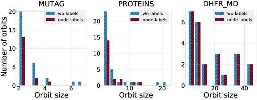
Figure 2: Examples of distributions of orbit sizes with node labels.

Sizes of the data sets. Another reason for having isomorphism in a data set is the sizes of graphs, which could be too small on average to lead to a diversity in a data set. In general, the number of non-isomorphic graphs with $n$ vertices and $m$ edges can be computed using Polya enumeration theory and grows very fast. For example, for a graph with 15 nodes and 15 edges, there are 2,632,420 non-isomorphic graphs. Nevertheless, specifics of the origin of the data set may affect possible configurations that graphs have (e.g. structure of chemical compounds in COX2_MD or ego-networks for actors in IMDB-BINARY) and thus smaller graphs may tend to be close to isomorphic structures. On the other hand, all five data sets with the average number of nodes greater than 100 have very low or zero proportion of isomorphic graphs. Hence, the average size of the graphs directly impacts the possible structure of the data set and thus data sets with larger graphs tend to be more diverse. We next analyze the consequences of the isomorphic graphs on classification methods.

6 Influence of isomorphism bias

To understand the impact of isomorphic graphs in the data set on the final metric we consider separately the results on two subparts of the data set. In particular, let $Y_{train}$ and $Y_{test}$ be train and test splits of a data set. Let $H_{i}\in Y_{test}$ be a graph such that there exists an isomorphic graph $G_{i}\in Y_{train}$ in the train data set. Let $\{Y_{iso}\}$ be a set of all such graphs $H_{i}$ for which there exists an isomorphic graph $G_{i}$ in $Y_{train}$. Note that the graphs in $\{Y_{iso}\}$ are not necessarily isomorphic. We denote by $Y_{new}$ the test graphs that do not have isomorphic copies in the train data set, i.e. $Y_{new}=Y_{test}\setminus Y_{iso}$. If we want to test generalization of classification models, we need to test it on new instances of the data sets and therefore at least consider $Y_{new}$ instead of $Y_{test}$. One question regarding the performance of the models on this new test set $Y_{new}$ is whether the performance on it will be lower than on the original test set $Y_{test}$. As we show below answer to this question solely depends on the accuracy of the model on isomorphic instances $Y_{iso}$.

Consider a graph classification model that is evaluated on normalized accuracy over a data set $Y$:

$${\text{acc}(Y)=\frac{\sum\limits_{G\in Y}\text{acc}(G_{i})}{|Y|}},$$ (1)

where $\text{acc}(G)$ equals to one if the model predicts the label of $G_{i}$ correctly, and zero otherwise. If $|Y|=0$, then we consider $\text{acc}(Y)=0$. We can see that the accuracy on the test data set can be written as the sum of two terms:

$$\begin{split}\text{acc}(Y_{test})&=\dfrac{\sum\limits_{G\in Y_{test}}\text{acc}(G)}{|Y_{test}|}=\dfrac{\sum\limits_{G\in Y_{new}}\text{acc}(G)+\sum\limits_{G\in Y_{iso}}\text{acc}(G)}{|Y_{test}|}=\\ &=\dfrac{|Y_{new}|}{|Y_{test}|}\text{acc}(Y_{new})+\dfrac{|Y_{iso}|}{|Y_{test}|}\text{acc}(Y_{iso}).\end{split}$$ (2)

Equation 2 decomposes accuracy on the original data set as the weighted sum of two accuracies on the set of the new test instances $Y_{new}$ and a set of the instances $Y_{iso}$ already appeared in the train set and therefore available to the model. We call the term $\text{acc}(Y_{iso})$ as isomorphism bias, which corresponds to the accuracy of the model on the isomorphic test instances. As we will see next, the accuracy of the model on the new set $Y_{new}$ will be less if only if the model performs better on the isomorphic set $Y_{iso}$.

Property 6.1.

Let $Y_{test}=Y_{new}\cup Y_{iso}$, $Y_{new}\cap Y_{iso}=\varnothing$ and $Y_{iso}\neq\varnothing$, where $Y_{iso}\subset Y_{train}$. Then for any classification model accuracy on the new test instances $Y_{new}$ is smaller than on the test set $Y_{test}$ if and only if it is smaller than accuracy on the isomorphic test instances $Y_{iso}$, i.e.:

$$\text{acc}(Y_{test})>\text{acc}(Y_{new})\iff\text{acc}(Y_{iso})>\text{acc}(Y_{new})$$ (3)

The equation 3 gives a definite answer with the possible performance of the model on a new test set. If the model performs well on isomorphic instances $Y_{iso}$, then it will falsely increase performance on $Y_{test}$ in comparison to $Y_{new}$. Conversely, if the model performs poorly on the instances that appeared in the training set, then removing them from the test set and evaluating the model purely on $Y_{new}$ will demonstrate higher accuracy. There are two reasons for the model to misclassify isomorphic instances $Y_{iso}$: (i) the instances contain target labels that are different than those that it has seen, as we show in Table 2 the percentage of mismatched labels can be high in some data sets; or (ii) the model is not expressive enough to map the structure of the graphs to the target label correctly.

Crucially, while $Y_{new}$ tests generalization capabilities of the models, on $Y_{iso}$ the models can explicitly or implicitly memorize the right labels from the training. We describe a model-agnostic way to guarantee increase of classification performance if $|Y_{iso}|\neq 0$.

Let $G\cong\widehat{G}$ such that $G\in Y_{iso}$ and $\widehat{G}\in Y_{train}$. Note that there can be multiple isomorphic graphs $\{\widehat{G}_{i}\}\subset Y_{train}$. If for any $G\in Y_{iso}$ all target labels of the orbit of $G$ are the same we call the set $Y_{iso}$ as homogeneous. Consider a classification model $\mathcal{M}$ that maps each graph $G$ to its label $l(G)$. We define a peering model $\widehat{\mathcal{M}}$ such that for each $G\in Y_{iso}$ it outputs the target label $l(\widehat{G})$. Then the accuracy of the model $\widehat{\mathcal{M}}$ is at least as the accuracy of the original model $\mathcal{M}$.

Theorem 6.1.

Let $Y_{test}=Y_{new}\cup Y_{iso}$, $Y_{new}\cap Y_{iso}=\varnothing$. If $Y_{iso}$ is homogeneous, then the accuracy on $Y_{test}$ of a classification model $\mathcal{M}$ is at most as the accuracy of its peering model $\hat{\mathcal{M}}$, i.e.:

$$\text{acc}_{\mathcal{M}}(Y_{test})\leq\text{acc}_{\widehat{\mathcal{M}}}(Y_{test}).$$

Theorem 6.1 establishes a way to increase performance only for homogeneous $Y_{iso}$. If there are noisy labels in the training set and hence the set is not homogeneous, the model cannot guarantee the right target label for these instances. Nonetheless, one can select a heuristic such as majority vote among the training isomorphic instances to select a proper label at the testing time.

In experiments, we compare neural network model (NN) [55] with graph kernels, Weisfeiler-Lehman (WL) [44] and vertex histogram (V) [47]. For each model we consider two modifications: one for peering model on homogeneous $Y_{iso}$ (e.g. NN-PH) and one for peering model on all $Y_{iso}$ (e.g. NN-P). We show accuracy on $Y_{test}$ and on $Y_{iso}$ (in brackets) in Table 4. Experimentation details can be found in Appendix G.

From Table 4 we can conclude that peering model on homogeneous data is always the top performer. This is aligned with the result of Theorem 6.1, which guarantees that $acc(Y_{iso})=1$, but it is an interesting observation if we compare it to the peering model on all isomorphic instances $Y_{iso}$ (-P models). Moreover, the latter model often loses even to the original model, where no information from the train set is explicitly taken into the test set. This can be explained by the noisy target labels in the orbits of isomorphic graphs, as can be seen both from the statistics for these datasets (Table 6) and accuracy measured just on isomorphic instances $Y_{iso}$. These results show that due to the presence of isomorphism bias performance of any classification model can be overestimated by as much as 5% of accuracy on these datasets and hence future comparison of classification models should be estimated on $Y_{new}$ instead.

Table 4: Mean classification accuracy for test sets $Y_{test}$ and $Y_{iso}$ (in brackets) in 10-fold cross-validation. Top-1 result in bold.

	MUTAG	IMDB-B	IMDB-M	COX2	AIDS	PROTEINS
NN	0.829 (0.840)	0.737 (0.733)	0.501 (0.488)	0.82 (0.872)	0.996 (0.998)	0.737 (0.834)
NN-PH	0.867 (1.000)	0.756 (1.000)	0.522 (1.000)	0.838 (1.000)	0.996 (1.000)	0.742 (1.000)
NN-P	0.856 (0.847)	0.737 (0.731)	0.499 (0.486)	0.795 (0.83)	0.996 (0.999)	0.729 (0.709)
WL	0.862 (0.867)	0.734 (0.990)	0.502 (0.953)	0.800 (0.974)	0.993 (0.999)	0.747 (0.950)
WL-PH	0.907 (1.000)	0.736 (1.000)	0.504 (1.000)	0.810 (1.000)	0.994 (1.000)	0.749 (1.000)
WL-P	0.870 (0.838)	0.724 (0.715)	0.495 (0.487)	0.794 (0.844)	0.994 (0.999)	0.740 (0.742)
V	0.836 (0.902)	0.707 (0.820)	0.503 (0.732)	0.781 (0.966)	0.994 (0.997)	0.726 (0.946)
V-PH	0.859 (1.000)	0.750 (1.000)	0.517 (1.000)	0.794 (1.000)	0.996 (1.000)	0.729 (1.000)
V-P	0.827 (0.844)	0.724 (0.728)	0.496 (0.481)	0.768 (0.852)	0.996 (0.999)	0.719 (0.741)

6.1 General recommendations

In order to avoid measuring performance over the wrong test sets, we provide a set of recommendations that will guarantee measuring the right metrics for the models.

• We open-source new, "clean" data sets that do not include isomorphic instances that are in Table 8. To tackle this problem in the future, we propose to use clean versions of the data set for which isomorphism bias vanishes. For each data set we consider the found graph orbits and keep only one graph from each orbit if and only if the graphs in the orbit have the same label. If the orbit contains more than one label, a classification model can do little to predict a correct label at the inference time and hence we remove such orbit completely. In this case, for a new data set $Y_{iso}=\varnothing$ and hence it prevents the models to implicitly memorize the labels from the training set. We consider the data set orbits that do not account for neither node nor edge labels because the remaining graphs are not isomorphic based purely on graph topology.

• Incorporating node and edge features into the models may be necessary to distinguish the graphs. As we have seen, just using node labels can reduce the number of isomorphic graphs significantly and many data sets provide additional information to distinguish the models at full scope.

• Verification of the models on bigger graphs in general is more challenging due to the sheer number of non-isomorphic graphs. For example, data sets related to REDDIT or DD include a number of big graphs for classification.

7 Conclusion

In this work we study isomorphism bias of the classification models in graph structured data that originates from substantial amount of isomorphic graphs in the data sets. We analyzed 54 graph data sets and provide the reasons for it as well as a set of rules to avoid unfair comparison of the models. We showed that in the current data sets any model can memorize the correct answers from the training set and we open-source new clean data sets where such problems does not appear.

Appendix A Statistics for original data sets

Table 5: All original graph data sets. $N$ is the number of graphs, $C$ is the number of different classes. Avg. Nodes and Avg. Edges is the average number of nodes and edges. N.L. and E.L indicate if the graphs in a data set contain node or edge labels.

data set	Type	$N$	$C$	Avg. Nodes	Avg. Edges	N.L.	E.L.	Source
FIRSTMM_DB	Molecular	41	11	1377.27	3074.1	+	-	[32]
OHSU	Molecular	79	2	82.01	199.66	+	-	[36]
KKI	Molecular	83	2	26.96	48.42	+	-	[36]
Peking_1	Molecular	85	2	39.31	77.35	+	-	[36]
MUTAG	Molecular	188	2	17.93	19.79	+	+	[23]
MSRC_21C	Vision	209	20	40.28	96.6	+	-	[32]
MSRC_9	Vision	221	8	40.58	97.94	+	-	[32]
Cuneiform	Molecular	267	30	21.27	44.8	+	+	[20]
SYNTHETIC	Synthetic	300	2	100	196	-	-	[8]
COX2_MD	Molecular	303	2	26.28	335.12	+	+	[23]
BZR_MD	Molecular	306	2	21.3	225.06	+	+	[23]
PTC_MM	Molecular	336	2	13.97	14.32	+	+	[23]
PTC_MR	Molecular	344	2	14.29	14.69	+	+	[23]
PTC_FM	Molecular	349	2	14.11	14.48	+	+	[23]
PTC_FR	Molecular	351	2	14.56	15	+	+	[23]
DHFR_MD	Molecular	393	2	23.87	283.01	+	+	[23]
Synthie	Synthetic	400	4	95	172.93	-	-	[30]
BZR	Molecular	405	2	35.75	38.36	+	-	[48]
ER_MD	Molecular	446	2	21.33	234.85	+	+	[23]
COX2	Molecular	467	2	41.22	43.45	+	-	[48]
DHFR	Molecular	467	2	42.43	44.54	+	-	[48]
MSRC_21	Vision	563	20	77.52	198.32	+	-	[32]
ENZYMES	Molecular	600	6	32.63	62.14	+	-	[4]
IMDB-BINARY	Social	1000	2	19.77	96.53	-	-	[56]
PROTEINS	Molecular	1113	2	39.06	72.82	+	-	[4]
DD	Molecular	1178	2	284.32	715.66	+	-	[43]
IMDB-MULTI	Social	1500	3	13	65.94	-	-	[56]
AIDS	Molecular	2000	2	15.69	16.2	+	+	[39]
REDDIT-BINARY	Social	2000	2	429.63	497.75	-	-	[56]
Letter-high	Molecular	2250	15	4.67	4.5	-	-	[39]
Letter-low	Molecular	2250	15	4.68	3.13	-	-	[39]
Letter-med	Molecular	2250	15	4.67	4.5	-	-	[39]
Fingerprint	Molecular	2800	4	5.42	4.42	-	-	[39]
COIL-DEL	Molecular	3900	100	21.54	54.24	-	+	[39]
COIL-RAG	Molecular	3900	100	3.01	3.02	-	-	[39]
NCI1	Molecular	4110	2	29.87	32.3	+	-	[43]
NCI109	Molecular	4127	2	29.68	32.13	+	-	[43]
FRANKENSTEIN	Molecular	4337	2	16.9	17.88	-	-	[35]
Mutagenicity	Molecular	4337	2	30.32	30.77	+	+	[39]
REDDIT-MULTI-5K	Social	4999	5	508.52	594.87	-	-	[56]
COLLAB	Social	5000	3	74.49	2457.78	-	-	[56]
Tox21_ARE	Molecular	7167	2	16.28	16.52	+	+	[7]
Tox21_aromatase	Molecular	7226	2	17.5	17.79	+	+	[7]
Tox21_MMP	Molecular	7320	2	17.49	17.83	+	+	[7]
Tox21_ER	Molecular	7697	2	17.58	17.94	+	+	[7]
Tox21_HSE	Molecular	8150	2	16.72	17.04	+	+	[7]
Tox21_AHR	Molecular	8169	2	18.09	18.5	+	+	[7]
Tox21_PPAR-gamma	Molecular	8184	2	17.23	17.55	+	+	[7]
Tox21_AR-LBD	Molecular	8599	2	17.77	18.16	+	+	[7]
Tox21_p53	Molecular	8634	2	17.79	18.19	+	+	[7]
Tox21_ER_LBD	Molecular	8753	2	18.06	18.47	+	+	[7]
Tox21_ATAD5	Molecular	9091	2	17.89	18.3	+	+	[7]
Tox21_AR	Molecular	9362	2	18.39	18.84	+	+	[7]
REDDIT-MULTI-12K	Social	11929	11	391.41	456.89	-	-	[56]

Appendix B Isomorphism metrics for all data sets

Table 6: Isomorphic metrics for all data sets. Sorting is based on the proportion of isomorphic graphs $I\%$. Num. orbits is the number of non-trivial orbits. $IP\%$ is the proportion of isomorphic pairs of graphs, Mismatched $\%$ is the proportion of mismatched labels.

data set	Size, $N$	Num. orbits	Iso. graphs, $I$	$I\%$	$IP\%$	Mismatched $\%$
SYNTHETIC	300	2	300	100	100	100
Cuneiform	267	8	267	100	20.46	100
Letter-low	2250	32	2245	99.78	8.72	96.22
DHFR_MD	393	25	392	99.75	6.87	94.91
COIL-RAG	3900	20	3890	99.74	25.22	99.31
COX2_MD	303	13	301	99.34	11.83	98.68
ER_MD	446	31	442	99.1	5.57	82.74
Fingerprint	2800	69	2774	99.07	16.86	89.29
BZR_MD	306	22	303	99.02	7.16	95.75
Letter-med	2250	39	2226	98.93	8.05	92.93
Letter-high	2250	94	2200	97.78	3.67	95.91
IMDB-MULTI	1500	100	1212	80.8	6.39	74.67
Tox21_ATAD5	9091	1461	6167	67.84	0.09	9.15
Tox21_PPAR-gamma	8184	1265	5513	67.36	0.1	7.77
Tox21_AR	9362	1519	6295	67.24	0.08	8
Tox21_p53	8634	1345	5800	67.18	0.09	11.28
Tox21_AR-LBD	8599	1354	5766	67.05	0.09	6.88
Tox21_MMP	7320	1138	4875	66.6	0.1	18.76
Tox21_HSE	8150	1218	5425	66.56	0.1	18.02
Tox21_ER_LBD	8753	1375	5791	66.16	0.09	12.41
Tox21_ER	7697	1203	5078	65.97	0.09	27.32
Tox21_AHR	8169	1299	5377	65.82	0.09	15.61
Tox21_aromatase	7226	1084	4727	65.42	0.1	5.07
Tox21_ARE	7167	1047	4682	65.33	0.11	26.45
AIDS	2000	371	1259	62.95	0.13	0.35
COX2	467	76	283	60.6	0.6	20.56
IMDB-BINARY	1000	117	579	57.9	0.67	31.8
FRANKENSTEIN	4337	574	2230	51.42	0.09	30.87
MUTAG	188	31	79	42.02	0.49	6.91
BZR	405	43	165	40.74	0.6	8.89
PTC_MM	336	42	132	39.29	0.46	23.21
PTC_MR	344	40	125	36.34	0.41	25
PTC_FM	349	39	124	35.53	0.39	23.5
DHFR	756	89	250	33.07	0.14	9.13
PTC_FR	351	36	116	33.05	0.37	20.51
Mutagenicity	4337	397	1274	29.38	0.03	13.1
COLLAB	5000	158	1077	21.54	0.11	6.68
COIL-DEL	3900	155	796	20.41	0.06	18.56
PROTEINS	1113	35	151	13.57	0.1	9.07
NCI1	4110	225	523	12.73	0.01	1.7
NCI109	4127	222	519	12.58	0.01	1.7
ENZYMES	600	6	10	1.67	0	0
REDDIT-BINARY	2000	3	4	0.2	0	0
REDDIT-MULTI-12K	11929	8	17	0.14	0	0.04
FIRSTMM_DB	41	1	0	0	0	0
OHSU	79	1	0	0	0	0
KKI	83	1	0	0	0	0
Peking_1	85	1	0	0	0	0
MSRC_21C	209	1	0	0	0	0
MSRC_9	221	1	0	0	0	0
Synthie	400	1	0	0	0	0
MSRC_21	563	1	0	0	0	0
DD	1178	1	0	0	0	0
REDDIT-MULTI-5K	4999	1	0	0	0	0

Appendix C Orbit size distribution for all data sets

In the plots 3, 4, 5 the sizes of orbits are presented for each data set. Empty plots correspond to data sets with no isomorphic graphs. Plots with just wo-labels correspond to cases when there are no node labels available for the graphs in a data set.

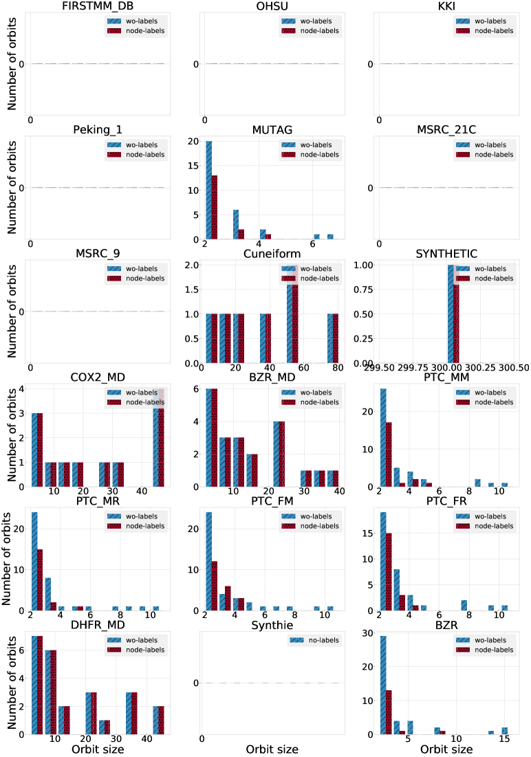
Figure 3: Distribution of orbits sizes. wo-labels correspond to isomorphism without considering the labels. node-labels correspond to isomorphism that considers node labels. Part-1.

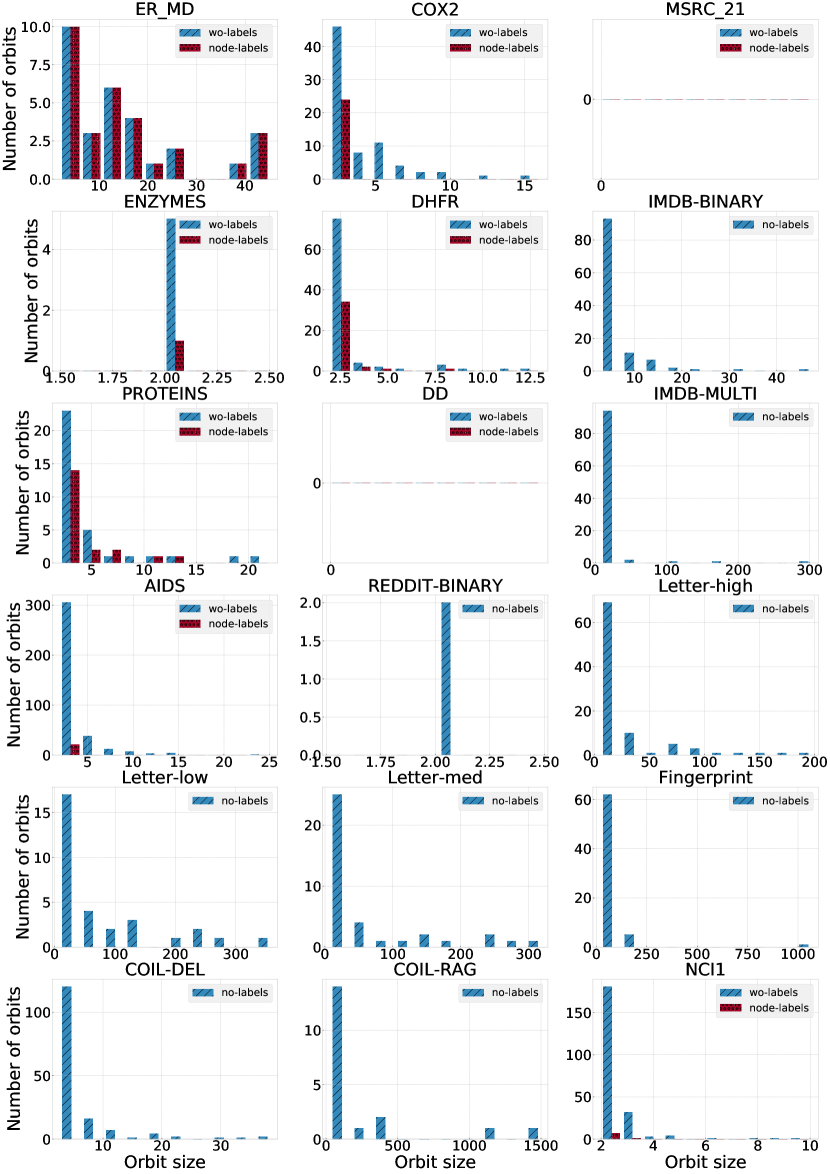
Figure 4: Distribution of orbits sizes. Part-2.

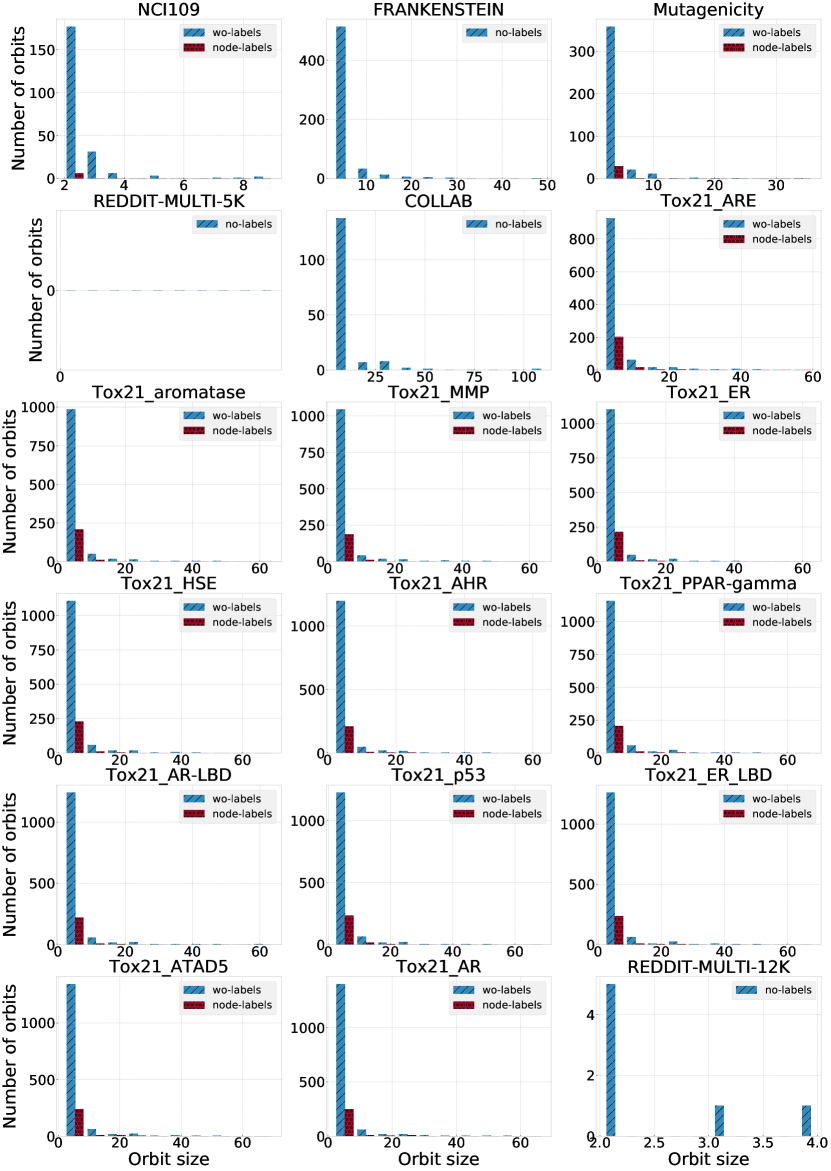
Figure 5: Distribution of orbits sizes. Part-3.

Appendix D Isomorphism metrics for data sets with node labels

Table 7: Isomorphic metrics for data sets with node labels. Sorting is based on the proportion of isomorphic graphs $I\%$. Num. orbits is the number of non-trivial orbits. $IP\%$ is the proportion of isomorphic pairs of graphs, Mismatched $\%$ is the proportion of mismatched labels. Table does not include data sets with no node labels.

data set	Size, $N$	Num. orbits	Iso. graphs, $I$	$I\%$	$IP\%$	Mismatched $\%$
SYNTHETIC	300	2	300	100	100	100
Cuneiform	267	8	267	100	20.46	100
DHFR_MD	393	25	392	99.75	6.87	94.91
COX2_MD	303	13	301	99.34	11.83	98.68
ER_MD	446	31	442	99.1	5.57	82.74
BZR_MD	306	22	303	99.02	7.16	95.75
MUTAG	188	17	36	19.15	0.14	0
PTC_FM	349	22	54	15.47	0.08	10.89
PTC_MM	336	22	50	14.88	0.07	7.74
DHFR	756	39	98	12.96	0.04	3.97
PTC_FR	351	20	43	12.25	0.05	6.27
PTC_MR	344	19	41	11.92	0.05	6.4
Tox21_ARE	7167	228	820	11.44	0.01	3.91
Tox21_HSE	8150	250	919	11.28	0.01	2.25
Tox21_aromatase	7226	223	805	11.14	0.01	0.77
Tox21_p53	8634	258	946	10.96	0.01	1.83
Tox21_ER	7697	231	840	10.91	0.01	2.4
COX2	467	25	50	10.71	0.03	1.07
Tox21_PPAR-gamma	8184	227	869	10.62	0.01	0.76
Tox21_MMP	7320	204	770	10.52	0.01	2.19
Tox21_ER_LBD	8753	255	913	10.43	0.01	1.28
Tox21_AR	9362	265	965	10.31	0.01	0.68
Tox21_ATAD5	9091	255	924	10.16	0.01	1.04
Tox21_AR-LBD	8599	238	871	10.13	0.01	0.7
BZR	405	16	40	9.88	0.06	0.99
Tox21_AHR	8169	224	795	9.73	0.01	2.07
PROTEINS	1113	21	74	6.65	0.03	2.61
AIDS	2000	22	54	2.7	0	0
Mutagenicity	4337	31	75	1.73	0	0.92
NCI1	4110	9	17	0.41	0	0.05
ENZYMES	600	2	2	0.33	0	0
NCI109	4127	7	12	0.29	0	0.05
FIRSTMM_DB	41	1	0	0	0	0
OHSU	79	1	0	0	0	0
KKI	83	1	0	0	0	0
Peking_1	85	1	0	0	0	0
MSRC_21C	209	1	0	0	0	0
MSRC_9	221	1	0	0	0	0
MSRC_21	563	1	0	0	0	0
DD	1178	1	0	0	0	0

Appendix E Proof of Property 6.1

Proof.

From the equation 2 we have:

$$\begin{split}&\text{acc}(Y_{test})=\dfrac{|Y_{new}|}{|Y_{test}|}\text{acc}(Y_{new})+\dfrac{|Y_{iso}|}{|Y_{test}|}\text{acc}(Y_{iso})>\text{acc}(Y_{iso})\Rightarrow\\[2.0pt] &\dfrac{|Y_{new}|}{|Y_{test}|}\text{acc}(Y_{new})>(1-\dfrac{|Y_{iso}|}{|Y_{test}|})\text{acc}(Y_{iso})\Rightarrow\\[2.0pt] &\text{acc}(Y_{iso})>\text{acc}(Y_{new})\end{split}$$

∎

Appendix F Proof of Theorem 6.1

Proof.

From the definition of the peering model we have:

$$\begin{split}&\text{acc}_{\mathcal{M}}(Y_{new})=\text{acc}_{\widehat{\mathcal{M}}}(Y_{new})\\[2.0pt] &\text{acc}_{\mathcal{M}}(Y_{iso})\leq\text{acc}_{\widehat{\mathcal{M}}}(Y_{iso})=1\end{split}$$

Substituting these into the equation 2 we have:

$$\text{acc}_{\mathcal{M}}(Y_{test})\leq\text{acc}_{\widehat{\mathcal{M}}}(Y_{test}).$$

∎

Appendix G Experimentation details

NN model is from [55] and evaluate it on the data sets from PyTorch-Geometric [10]. For each data set we perform 10-fold cross-validation such that each fold is evaluated on 10% of hold-out instances $Y_{test}$. For each fold we train the model for 350 epochs selecting the final model with the best performance on the validation set (20% from hold-out trained split) across all epochs. Additionally we found that for small data set performance during the first epochs can be unstable on the validation set and thus we select our model only after the first 50 epochs. The final model is evaluated on the test instances and corresponds to NN in the experiments. Peering models NN-PH and NN-P are obtained from NN by replicating the target labels for homogeneous $Y_{iso}$ and non-homogeneous $Y_{iso}$ respectively. Weisfeiler-Lehman and Vertex histogram kernels are taken from the code of [47]. We selected the height of subtree $h=5$ for WL kernel. We train an SVM model selecting $C$ parameter from the range [0.001, 0.01, 0.1, 1, 10].

Appendix H New data sets

Table 8: Statistics for new clean data sets. Retention is the proportion of graphs remaining after cleaning procedure. Min. Class and Max. Class are minimum and maximum number of graphs in a class. Sorted by retention.

Data set	Size	Retention, %	Avg. Nodes	Avg. Edges	Classes	Min. Class	Max. Class
SYNTHETIC	0	0	0	0	0	0	0
Cuneiform	0	0	0	0	0	0	0
COIL-RAG	13	0.33	5.77	9.62	7	1	5
Letter-low	12	0.53	7.17	5.42	5	1	3
COX2_MD	3	0.99	30.33	467	2	1	2
DHFR_MD	4	1.02	25.25	366.25	2	1	3
Letter-med	29	1.29	6.83	5.66	8	1	10
Fingerprint	51	1.82	14.45	13.12	6	1	40
BZR_MD	6	1.96	14.17	130.17	2	1	5
Letter-high	60	2.67	7.03	7.23	7	1	32
ER_MD	14	3.14	18.07	227.36	2	1	13
IMDB-MULTI	321	21.4	22.35	249.46	3	85	144
Tox21_ARE	3302	46.07	20.96	21.86	2	602	2700
Tox21_ER	3560	46.25	22.24	23.29	2	419	3141
Tox21_MMP	3405	46.52	22.4	23.43	2	618	2787
Tox21_HSE	3814	46.8	21.29	22.28	2	207	3607
Tox21_p53	4088	47.35	22.62	23.72	2	291	3797
Tox21_PPAR-gamma	3877	47.37	21.91	22.91	2	120	3757
Tox21_ATAD5	4312	47.43	22.52	23.61	2	168	4144
Tox21_AR-LBD	4134	48.08	22.41	23.48	2	150	3984
Tox21_AR	4506	48.13	22.93	24.05	2	189	4317
Tox21_AHR	3935	48.17	22.88	23.98	2	490	3445
Tox21_ER_LBD	4224	48.26	22.69	23.8	2	193	4031
Tox21_aromatase	3524	48.77	22.24	23.22	2	234	3290
IMDB-BINARY	493	49.3	24.08	221.96	2	232	261
COX2	237	50.75	42.14	44.43	2	68	169
AIDS	1110	55.5	18.22	19.1	2	310	800
FRANKENSTEIN	2448	56.44	20.78	22.35	2	1020	1428
PTC_MM	226	67.26	17.04	17.74	2	77	149
BZR	276	68.15	36.25	38.81	2	72	204
PTC_MR	235	68.31	17.23	17.97	2	96	139
PTC_FM	242	69.34	16.96	17.66	2	85	157
MUTAG	135	71.81	18.85	20.84	2	42	93
PTC_FR	253	72.08	17.11	17.86	2	86	167
DHFR	578	76.46	43.37	45.53	2	205	373
Mutagenicity	3335	76.9	32.96	34.16	2	1484	1851
COIL-DEL	3133	80.33	25.05	64.26	98	1	39
COLLAB	4064	81.28	76.94	4667.92	3	770	2289
PROTEINS	975	87.6	43.41	81.04	2	343	632
NCI1	3785	92.09	29.84	32.37	2	1781	2004
NCI109	3801	92.1	29.66	32.22	2	1801	2000
ENZYMES	595	99.17	32.48	62.17	6	98	100
REDDIT-BINARY	1998	99.9	430.04	996.48	2	998	1000
REDDIT-MULTI-12K	11917	99.9	391.79	914.68	11	513	2586
FIRSTMM_DB	41	100	1377.27	3073.93	11	2	6
OHSU	79	100	82.01	199.66	2	35	44
KKI	83	100	26.96	48.42	2	37	46
Peking_1	85	100	39.31	77.35	2	36	49
MSRC_21C	209	100	40.28	96.6	17	1	29
MSRC_9	221	100	40.58	97.94	8	19	30
Synthie	400	100	91.6	202.18	4	90	110
MSRC_21	563	100	77.52	198.32	20	10	34
DD	1178	100	284.32	715.66	2	487	691
REDDIT-MULTI-5K	4999	100	508.51	1189.75	5	999	1000

References

- [1] László Babai “Graph Isomorphism in Quasipolynomial Time” In CoRR abs/1512.03547, 2015 URL: http://arxiv.org/abs/1512.03547
- [2] Björn Barz and Joachim Denzler “Do we train on test data? Purging CIFAR of near-duplicates” In arXiv preprint arXiv:1902.00423, 2019
- [3] Vighnesh Birodkar, Hossein Mobahi and Samy Bengio “Semantic Redundancies in Image-Classification Datasets: The 10% You Don’t Need” In arXiv preprint arXiv:1901.11409, 2019
- [4] Karsten M Borgwardt, Cheng Soon Ong, Stefan Schönauer, SVN Vishwanathan, Alex J Smola and Hans-Peter Kriegel “Protein function prediction via graph kernels” In Bioinformatics 21.suppl_1 Oxford University Press, 2005, pp. i47–i56
- [5] Jin-Yi Cai, Martin Fürer and Neil Immerman “An optimal lower bound on the number of variables for graph identification” In Combinatorica 12.4 Springer, 1992, pp. 389–410
- [6] Jin-yi Cai, Martin Fürer and Neil Immerman “An optimal lower bound on the number of variables for graph identifications” In Combinatorica, 1992
- [7] Tox21 Data Challenge “Tox21 Data Challenge 2014”, 2014 URL: https://tripod.nih.gov/tox21/challenge/data.jsp
- [8] Aasa Feragen, Niklas Kasenburg, Jens Petersen, Marleen Bruijne and Karsten Borgwardt “Scalable kernels for graphs with continuous attributes” In Advances in Neural Information Processing Systems, 2013, pp. 216–224
- [9] Grégoire Ferré, Terry Haut and Kipton Barros “Learning molecular energies using localized graph kernels” In The Journal of chemical physics 146.11 AIP Publishing, 2017, pp. 114107
- [10] Matthias Fey and Jan E. Lenssen “Fast Graph Representation Learning with PyTorch Geometric” In ICLR Workshop on Representation Learning on Graphs and Manifolds, 2019
- [11] Martin Fürer “On the combinatorial power of the Weisfeiler-Lehman algorithm” In International Conference on Algorithms and Complexity, 2017, pp. 260–271 Springer
- [12] Thomas Gärtner, Peter Flach and Stefan Wrobel “On graph kernels: Hardness results and efficient alternatives” In Learning theory and kernel machines Springer, 2003, pp. 129–143
- [13] Goran Glavaš and Jan Šnajder “Event-centered information retrieval using kernels on event graphs” In Proceedings of TextGraphs-8 Graph-based Methods for Natural Language Processing, 2013, pp. 1–5
- [14] J.. Hopcroft and J.. Wong “Linear Time Algorithm for Isomorphism of Planar Graphs (Preliminary Report)” In Proceedings of the Sixth Annual ACM Symposium on Theory of Computing, STOC ’74, 1974
- [15] Sergey Ivanov and Evgeny Burnaev “Anonymous Walk Embeddings” In Proceedings of the 35th International Conference on Machine Learning (ICML), 2018
- [16] Biao Jie, Mingxia Liu, Xi Jiang and Daoqiang Zhang “Sub-network based kernels for brain network classification” In Proceedings of the 7th ACM International Conference on Bioinformatics, Computational Biology, and Health Informatics, 2016, pp. 622–629 ACM
- [17] Fredrik Johansson, Vinay Jethava, Devdatt Dubhashi and Chiranjib Bhattacharyya “Global graph kernels using geometric embeddings” In Proceedings of the 31st International Conference on Machine Learning, ICML 2014, Beijing, China, 21-26 June 2014, 2014
- [18] Paul J. Kelly “A congruence theorem for trees.” In Pacific J. Math. 7.1 Pacific Journal of Mathematics, A Non-profit Corporation, 1957, pp. 961–968 URL: https://projecteuclid.org:443/euclid.pjm/1103043674
- [19] Kristian Kersting, Nils M. Kriege, Christopher Morris, Petra Mutzel and Marion Neumann “Benchmark Data Sets for Graph Kernels”, 2016 URL: http://graphkernels.cs.tu-dortmund.de
- [20] Nils M Kriege, Matthias Fey, Denis Fisseler, Petra Mutzel and Frank Weichert “Recognizing cuneiform signs using graph based methods” In arXiv preprint arXiv:1802.05908, 2018
- [21] Nils M Kriege, Fredrik D Johansson and Christopher Morris “A Survey on Graph Kernels” In arXiv preprint arXiv:1903.11835, 2019
- [22] Nils M Kriege, Christopher Morris, Anja Rey and Christian Sohler “A Property Testing Framework for the Theoretical Expressivity of Graph Kernels.” In IJCAI, 2018, pp. 2348–2354
- [23] Nils Kriege and Petra Mutzel “Subgraph matching kernels for attributed graphs” In arXiv preprint arXiv:1206.6483, 2012
- [24] Kousik Kundu, Fabrizio Costa and Rolf Backofen “A graph kernel approach for alignment-free domain–peptide interaction prediction with an application to human SH3 domains” In Bioinformatics 29.13 Oxford University Press, 2013, pp. i335–i343
- [25] Wenchao Li, Hassen Saidi, Huascar Sanchez, Martin Schäf and Pascal Schweitzer “Detecting similar programs via the Weisfeiler-Leman graph kernel” In International Conference on Software Reuse, 2016, pp. 315–330 Springer
- [26] Eugene M. Luks “Isomorphism of Graphs of Bounded Valence Can Be Tested in Polynomial Time” In Proceedings of the 21st Annual Symposium on Foundations of Computer Science, SFCS ’80, 1980
- [27] Haggai Maron, Heli Ben-Hamu, Hadar Serviansky and Yaron Lipman “Provably Powerful Graph Networks” In arXiv preprint arXiv:1905.11136, 2019
- [28] Brendan D. Mckay and Adolfo Piperno “Practical Graph Isomorphism, II” In J. Symb. Comput., 2014
- [29] Silvio Micali and Zeyuan Allen Zhu “Reconstructing Markov processes from independent and anonymous experiments” In Discrete Applied Mathematics 200, 2016, pp. 108–122
- [30] Christopher Morris, Nils M Kriege, Kristian Kersting and Petra Mutzel “Faster kernels for graphs with continuous attributes via hashing” In 2016 IEEE 16th International Conference on Data Mining (ICDM), 2016, pp. 1095–1100 IEEE
- [31] Christopher Morris, Martin Ritzert, Matthias Fey, William L Hamilton, Jan Eric Lenssen, Gaurav Rattan and Martin Grohe “Weisfeiler and leman go neural: Higher-order graph neural networks” In Proceedings of the AAAI Conference on Artificial Intelligence 33, 2019, pp. 4602–4609
- [32] Marion Neumann, Roman Garnett, Christian Bauckhage and Kristian Kersting “Propagation kernels: efficient graph kernels from propagated information” In Machine Learning 102.2 Springer, 2016, pp. 209–245
- [33] Giannis Nikolentzos, Giannis Siglidis and Michalis Vazirgiannis “Graph Kernels: A Survey” In arXiv preprint arXiv:1904.12218, 2019
- [34] Luca Oneto, Nicolò Navarin, Michele Donini, Alessandro Sperduti, Fabio Aiolli and Davide Anguita “Measuring the expressivity of graph kernels through statistical learning theory” In Neurocomputing 268 Elsevier, 2017, pp. 4–16
- [35] Francesco Orsini, Paolo Frasconi and Luc De Raedt “Graph invariant kernels” In Twenty-Fourth International Joint Conference on Artificial Intelligence, 2015
- [36] Shirui Pan “A Repository of Benchmark Graph Datasets for Graph Classification”, 2018 URL: https://github.com/shiruipan/graph_datasets
- [37] Liva Ralaivola, Sanjay J Swamidass, Hiroto Saigo and Pierre Baldi “Graph kernels for chemical informatics” In Neural networks 18.8 Elsevier, 2005, pp. 1093–1110
- [38] Benjamin Recht, Rebecca Roelofs, Ludwig Schmidt and Vaishaal Shankar “Do ImageNet Classifiers Generalize to ImageNet?” In arXiv preprint arXiv:1902.10811, 2019
- [39] Kaspar Riesen and Horst Bunke “IAM graph database repository for graph based pattern recognition and machine learning” In Joint IAPR International Workshops on Statistical Techniques in Pattern Recognition (SPR) and Structural and Syntactic Pattern Recognition (SSPR), 2008, pp. 287–297 Springer
- [40] Matthias Rupp and Gisbert Schneider “Graph kernels for molecular similarity” In Molecular Informatics 29.4 Wiley Online Library, 2010, pp. 266–273
- [41] Franco Scarselli, Ah Chung Tsoi and Markus Hagenbuchner “The Vapnik–Chervonenkis dimension of graph and recursive neural networks” In Neural Networks 108 Elsevier, 2018, pp. 248–259
- [42] Maksim Sharaev, Alexey Artemov, Ekaterina Kondrateva, Sergei Ivanov, Svetlana Sushchinskaya, Alexander Bernstein, Andrzej Cichocki and Evgeny Burnaev “Learning connectivity patterns via graph kernels for fmri-based depression diagnostics” In 2018 IEEE International Conference on Data Mining Workshops (ICDMW), 2018, pp. 308–314 IEEE
- [43] Nino Shervashidze, Pascal Schweitzer, Erik Jan van Leeuwen, Kurt Mehlhorn and Karsten M Borgwardt “Weisfeiler-lehman graph kernels” In Journal of Machine Learning Research 12.Sep, 2011, pp. 2539–2561
- [44] Nino Shervashidze, Pascal Schweitzer, Erik Jan Leeuwen, Kurt Mehlhorn and Karsten M. Borgwardt “Weisfeiler-Lehman Graph Kernels” In Journal of Machine Learning Research 12, 2011, pp. 2539–2561
- [45] Nino Shervashidze, S… Vishwanathan, Tobias Petri, Kurt Mehlhorn and Karsten M. Borgwardt “Efficient graphlet kernels for large graph comparison” In Proceedings of the Twelfth International Conference on Artificial Intelligence and Statistics, AISTATS 2009, Clearwater Beach, Florida, USA, April 16-18, 2009, 2009, pp. 488–495
- [46] Elena Stumm, Christopher Mei, Simon Lacroix, Juan Nieto, Marco Hutter and Roland Siegwart “Robust visual place recognition with graph kernels” In Proceedings of the IEEE Conference on Computer Vision and Pattern Recognition, 2016, pp. 4535–4544
- [47] Mahito Sugiyama and Karsten Borgwardt “Halting in random walk kernels” In Advances in neural information processing systems, 2015, pp. 1639–1647
- [48] Jeffrey J Sutherland, Lee A O’brien and Donald F Weaver “Spline-fitting with a genetic algorithm: A method for developing classification structure- activity relationships” In Journal of chemical information and computer sciences 43.6 ACS Publications, 2003, pp. 1906–1915
- [49] Saurabh Verma and Zhi-Li Zhang “Stability and Generalization of Graph Convolutional Neural Networks” In arXiv preprint arXiv:1905.01004, 2019
- [50] S… Vishwanathan, Nicol N. Schraudolph, Risi Kondor and Karsten M. Borgwardt “Graph Kernels” In J. Mach. Learn. Res. 11 JMLR.org, 2010, pp. 1201–1242
- [51] Jianjia Wang, Richard C Wilson and Edwin R Hancock “fMRI activation network analysis using bose-einstein entropy” In Joint IAPR International Workshops on Statistical Techniques in Pattern Recognition (SPR) and Structural and Syntactic Pattern Recognition (SSPR), 2016, pp. 218–228 Springer
- [52] Harry Wiener “Correlation of heats of isomerization, and differences in heats of vaporization of isomers, among the paraffin hydrocarbons” In Journal of the American Chemical Society 69.11 ACS Publications, 1947, pp. 2636–2638
- [53] Harry Wiener “Influence of interatomic forces on paraffin properties” In The Journal of Chemical Physics 15.10 AIP, 1947, pp. 766–766
- [54] Zonghan Wu, Shirui Pan, Fengwen Chen, Guodong Long, Chengqi Zhang and Philip S Yu “A comprehensive survey on graph neural networks” In arXiv preprint arXiv:1901.00596, 2019
- [55] Keyulu Xu, Weihua Hu, Jure Leskovec and Stefanie Jegelka “How powerful are graph neural networks?” In arXiv preprint arXiv:1810.00826, 2018
- [56] Pinar Yanardag and SVN Vishwanathan “Deep graph kernels” In Proceedings of the 21th ACM SIGKDD International Conference on Knowledge Discovery and Data Mining, 2015, pp. 1365–1374 ACM
- [57] Rex Ying, Dylan Bourgeois, Jiaxuan You, Marinka Zitnik and Jure Leskovec “GNN Explainer: A Tool for Post-hoc Explanation of Graph Neural Networks” In arXiv preprint arXiv:1903.03894, 2019