Necessary Conditions
In Infinite-Horizon Control Problems
That Need No Asymptotic Assumptions

Abstract

We consider an infinite-horizon optimal control problem with an asymptotic terminal constraint. For the the weakly overtaking criterion and the overtaking criterion, necessary boundary conditions on co-state arcs are deduced, these conditions need no assumptions about the asymptotic behavior of the motion, co-state arc, cost functional, and its derivatives. In the absence of an asymptotic terminal constraint, these boundary conditions with the Pontryagin Maximum Principle allow raising the co-state arcs, corresponding to some asymptotic subdifferentials of the cost functional (fixing the optimal control) at infinity. If this set is a singleton, these conditions coincide with the co-state arc representation proposed by Aseev and Kryazhimskii. These results are illustrated by several examples.

Keywords: Infinite-horizon control problem, Pontryagin maximum principle, overtaking optimal control, transversality condition at infinity, convergence of subdifferentials, optimal growth

MSC2010 49K15, 49J53, 93C15

1 Introduction

We will consider an infinite-horizon optimal control problem,

minimize $$l(y(0))+\int_{0}^{\infty}f_{0}(\tau,y(\tau),u(\tau))\,d\tau$$

subject to $$\frac{d{y}(t)}{dt}=f(t,y(t),u(t))\quad\textrm{a.e.},$$

$$y(t)\in\mathbb{R}^{m},\ u(t)\in U,\ y(0)\in\mathcal{C}_{0},\ \operatorname*{Limsup}_{\theta\uparrow\infty}\{\Lambda(\theta,y(\theta))\}\subset\mathcal{C}_{\infty}$$

with the relations of the Pontryagin Maximum Principle corresponding to this problem:

$$\frac{d{y}(t)}{dt} = f\big{(}t,y(t),{u}(t)\big{)},$$ (1a)

$$-\frac{d{\psi}(t)}{dt} = \frac{\partial{H}}{\partial x}\big{(}y(t),\psi(t),{u}(t),\lambda,t\big{)},$$ (1b)

$$\sup_{\upsilon\in U}H\big{(}y(t),\psi(t),\upsilon,\lambda,t\big{)} = H\big{(}y(t),\psi(t),{u}(t),\lambda,t\big{)}.$$ (1c)

Here, ${\mathbb{R}}_{+}\stackrel{{\scriptstyle\triangle}}{{=}}[0;\infty)$ is the time interval of the control system, the sets $\mathcal{C}_{0}$ and $\mathcal{C}_{\infty}$ are nonempty subsets of $\mathbb{X}\stackrel{{\scriptstyle\triangle}}{{=}}\mathbb{R}^{m}$, $l$ and $\Lambda$ is a scalar function on $\mathbb{X}$, the set $U$ of control parameters is a nonempty subset of a certain finite-dimensional real vector space, and the Hamilton–Pontryagin function $H:{\mathbb{X}}\times{\mathbb{X}}^{*}\times{U}\times{\mathbb{R}_{+}}\times{\mathbb{R}_{+}}\to{\mathbb{R}}$ is given by

$$H(x,\psi,u,\lambda,t)\stackrel{{\scriptstyle\triangle}}{{=}}\psi f\big{(}t,x,u\big{)}-\lambda f_{0}\big{(}t,x,u\big{)}\quad\forall(x,\psi,u,\lambda,t)\in{\mathbb{X}}\times{\mathbb{X}}^{*}\times{U}\times{\mathbb{R}_{+}}\times{\mathbb{R}_{+}}.$$

It is well known that the relations (1a)–(1c) are necessary conditions for finite-horizon control problems [39]. For infinite-horizon control problems, the Pontryagin Maximum Principle was proved in the pioneering paper [25] in the case of the finite optimality criterion (the optimality on each finite interval of the corresponding problem with fixed ends). In this sense, each optimal process as an extension of optimal processes for the finite horizon problems admits the extension of (1a)-(1c) from each finite interval to $\mathbb{R}_{+}$. By passing to the limit, one obtains the necessary conditions on the whole $\mathbb{R}_{+}$, system (1a)–(1c) and the usual transversality condition at zero.

Naturally, on the one hand, this proof does not require any supplementary information on system (1a)–(1c) at infinity; on the other hand, nor is any such knowledge gained. In particular, this system of necessary relations lacks one more boundary condition on the co-state arc, which corresponds to the transversality condition at the right end. In fact, without such a condition, relations (1a)–(1c) only serve to point towards the variety of their solutions without offering a tool to choose one from among them.

To limit the search, various supplementary conditions are used; otherwise, in each specific problem, one could exhaustively search through all solutions [47]. The limit value at infinity for the motion itself can be specified [39, Subsect. 4.24]. The solution and/or control lie in a certain class of functions (see [6, 15, 50, 51]). It is also possible to connect some condition with the value function [41, 30, 16]. One can try to apply some relations due to economic reasons [44] and ones of convexity [43] and stability [49, 46]. Nevertheless, some supplementary information (in the form of boundary conditions) can be also tried to reclaim from a certain optimality criterion. In this paper, we obtain such conditions for rather mild optimality criteria such as the weakly overtaking criterion and the overtaking criterion (the optimality for the upper and lower pointwise limits of the cost functional, respectively).

In [42], the necessary conditions, including a complete set of transversality conditions for the co-state arc at infinity, were considered. In the case of a final state dependent cost functional, as well as of an asymptotic terminal constraint of a linear structure, these conditions were proved under very strong asymptotic assumptions on motions and costs. In [37, 51], a similar result was shown under some asymptotic assumptions, guaranteeing the existence of the limit of motions. In [31], the necessary transversality condition was obtained as a consequence of the stability of the limiting subdifferentials with respect to the uniform convergence. In this paper, this approach is applied to the derivation of necessary conditions based on the stability of subdifferentials. It makes it possible, while continuing to follow Halkin’s method, to reformulate the overtaking criterion in these terms, and pass to the limit within the necessary conditions for specially selected problems for the increasing sequence of time intervals.

Adhering to this approach, we apply the classical results [21] with respect to the Fréchet subdifferential for the epigraphical convergence and refine the upper-estimates [33, Theorem 6.2] of the limiting subdifferential of the pointwise lower and upper limit (see Lemmata 5 and 6). Further, we apply these estimates directly to the transversality condition of the classical Pontryagin Maximum Principle [18, 52] for some Bolza problems for the increasing sequence of time intervals. Thus, we establish the necessary conditions for the weakly overtaking and overtaking criteria (see Theorems 1 and 2), which notably require no asymptotic assumptions on the motion, cost functional, adjoint variable, and its gradients.

A special focus of this paper is the question of the accuracy of the considered transversality conditions at infinity for the problem without asymptotic constraint. If the cost functional gradients have a limit for large time, the proposed transversality condition (11a) is explicit, i.e. it points to a unique solution to the adjoint system of (1b); moreover, this solution coincides with the co-state arc representation [2] proposed by Kryazhimskii and Aseev. On the other hand, in the case of the periodic functional, even for an infinite-horizon control problem linear in $x$ (see Example 5), there is no hope to construct any explicit boundary condition on $\psi$ necessary for the weakly overtaking optimal criterion; each such condition is going to contain a ball. At the same time, in this example, the proposed condition (11a) is the strongest of all consistent with (1c) boundary conditions on the co-state arc.

The rest of the paper is organised as follows. First, we introduce the statement of the infinite-horizon control problem, the dynamics and cost functional, and formulate the basic hypotheses on them; we also define all needed optimality criteria. In Section 3, we recall the concepts and notions of set-valued and variational analyses. Section 4 exhibits formulations of all theorems and corollaries and the discussion of their assumptions and conditions. The subsequent section is devoted to examples. Subdifferentials of lower and upper limits of functions defined on finite-dimensional sets are considered in Section 6. The last part of the paper (Section 7) contains the proofs of all theorems.

2 The statement of the infinite-horizon control problem

Let ${\mathbb{R}}_{+}=[0;\infty)$ be the time interval of an investigated control system, and let ${\mathbb{X}}={\mathbb{R}}^{m}$ be its state space. Let functions $l:\mathbb{X}\to\mathbb{R}$, $\Lambda:\mathbb{R}_{+}\times\mathbb{X}\to\mathbb{X}$ and nonempty sets $\mathcal{C}_{0}\subset{\mathbb{X}}$, $\mathcal{C}_{\infty}\subset{\mathbb{X}}$ be given. Let a non-empty subset $U$ of a finite-dimensional real vector space also be given; denote by $\mathcal{U}$ the set of all admissible controls, all Lebesgue measurable functions $u:\mathbb{R}_{+}\to U$.

Consider the following infinite-horizon optimal control problem:

minimize $$l(y(0))+\int_{0}^{\infty}f_{0}(\tau,y(\tau),u(\tau))\,d\tau$$ (2a)

subject to $$\frac{d{y}(t)}{dt}=f(t,y(t),u(t))\ \quad\textrm{a.e.},$$ (2b)

$$y(t)\in\mathbb{X}=\mathbb{R}^{m},\ y(0)\in\mathcal{C}_{0},\ \operatorname*{Limsup}_{\theta\uparrow\infty}\{\Lambda(\theta,y(\theta))\}\subset\mathcal{C}_{\infty},\ u\in\mathcal{U},$$ (2c)

here the symbol $\operatorname*{Limsup}$ is defined in Section 3, see (6).

Hereinafter, we assume the following conditions to hold:

• $l:\mathbb{X}\to\mathbb{R}$ is a locally Lipschitz continuous function;

• $f:\mathbb{R}_{+}\times\mathbb{X}\times U\to\mathbb{X}$ and $f_{0}:\mathbb{R}_{+}\times\mathbb{X}\times U\to\mathbb{R}$ are LB measurable in $(t,u)$.

For every compact interval $I\subset\mathbb{R}_{+}$ a pair $(y,u)\in(AC)(I,\mathbb{X})\times{\mathcal{U}}$ is called a control process if the map $I\ni\tau\mapsto f_{0}\big{(}\tau,y(\tau),u(\tau)\big{)}$ is summable and $y$ is a solution to equation (2b) on $I$, i.e., (2b) holds for almost all $t\in I$. A pair $({y},{u})\in(AC)(\mathbb{R}_{+},\mathbb{X})\times{\mathcal{U}}$ is called admissible control process if $y$ satisfies (2c) and the pair $({y}|_{[0;T]},{u})$ is a control process for every $T>0$.

We will use the following optimality criteria:

Definition 1.

Call an admissible control process $({\hat{y}},{\hat{u}})$ overtaking optimal [49, 17] for problem (2a)–(2c) if for every admissible control process $(y,u)$ it holds that

$$l(y(0))-l({\hat{y}}(0))+\liminf_{\theta\uparrow\infty}\int_{0}^{\theta}\big{[}f_{0}(\tau,y(\tau),u(\tau))-f_{0}(\tau,{\hat{y}}(\tau),{\hat{u}}(\tau))\big{]}\,d\tau\geq 0.$$ (3a)

Definition 2.

Call an admissible control process $({\hat{y}},{\hat{u}})$ weakly overtaking optimal [49, 17] for problem (2a)–(2c) if for every admissible control process $(y,u)$ it holds that

$$l(y(0))-l({\hat{y}}(0))+\limsup_{\theta\uparrow\infty}\int_{0}^{\theta}\big{[}f_{0}(\tau,y(\tau),u(\tau))-f_{0}(\tau,{\hat{y}}(\tau),{\hat{u}}(\tau))\big{]}\,d\tau\geq 0.$$ (3b)

Clearly, an overtaking optimal process is weakly overtaking optimal, but we will relax the both criteria, considering merely its local variants [4, 45]:

Definition 3.

Call an admissible control process $({\hat{y}},{\hat{u}})$ locally overtaking (locally weakly overtaking) optimal for problem (2a)–(2c) if for every natural $n$ there exists a positive $\beta(n)$ such that, for each admissible control process $(y,u)$, from

$$\max_{t\in[0;n]}||y(t)-{\hat{y}}(t)||+\operatorname*{meas}\{t\in[0;n]\mid u(t)\neq{\hat{u}}(t)\}<\beta(n)$$ (4)

and ${u|_{[n;\infty)}={\hat{u}}|_{[n;\infty)}}$ there follows inequality (3a) (inequality (3b)).

Some conditions for the existence of weakly overtaking optimal and overtaking optimal processes are given in [8, 20, 12]. In this paper, the existence theory is not directly concerned. We also do not concern ourselves with sufficient optimality conditions (see [43, 49, 3, 41, 11]).

We assume that a certain admissible control process $({\hat{y}},{\hat{u}})$ is locally weakly overtaking optimal for problem (2a)–(2c). We will also assume several local assumptions on $({\hat{y}},{\hat{u}})$, hypotheses $(H2)$–$(H4)$. Note that from [18, Hypothesis 22.25] for each interval $[0;T]$ it follows hypotheses $(H2)$–$(H3)$. Besides, the hypothesis $(H4)$ requires merely the well-posedness of the right side of (1b) on the graph of optimal process $({\hat{y}},{\hat{u}})$.

Hereinafter, we assume that

• for each control parameter $\upsilon\in U$, there exist a neighbourhood $\mathbb{G}_{\upsilon}\subset\mathbb{R}_{+}\times\mathbb{X}$ of the graph of ${\hat{y}}$ and a measurable function $L_{\upsilon}:\mathbb{R}_{+}\to\mathbb{R}_{+}$ such that for all $(t,x^{\prime})$, $(t,x^{\prime\prime})\in\mathbb{G}_{\upsilon}$ one has

  $$\big{\|}f(t,x^{\prime},\upsilon)-{f}(t,x^{\prime\prime},\upsilon)\big{\|}+\big{\|}{f_{0}}(t,x^{\prime},\upsilon)-{f_{0}}(t,x^{\prime\prime},\upsilon)\big{\|}\leq L_{\upsilon}(t)\|x^{\prime}-x^{\prime\prime}\|;$$ (5)

• there exists a neighbourhood ${\hat{\mathbb{G}}}\subset\mathbb{R}_{+}\times\mathbb{X}$ of the graph of ${\hat{y}}$ such that, for all $(t,x^{\prime})$, $(t,x^{\prime\prime})\in{\hat{\mathbb{G}}}$, inequality (5) holds with $L_{{\hat{u}}(t)}(t)$ and ${\hat{u}}(t)$ instead of $L_{\upsilon}(t)$ and $\upsilon$; furthermore, the map $\mathbb{R}_{+}\ni t\mapsto L_{{\hat{u}}(t)}(t)$ is locally summable (summable on each compact interval);

• for almost all nonnegative $t$ the maps $x\mapsto f(t,x,{\hat{u}}(t))$ and $x\mapsto f_{0}(t,x,{\hat{u}}(t))$ are strictly differentiable (in $x$) at ${\hat{y}}(t)$.

For each admissible control $u\in{\mathcal{U}}$ and $(t,x)\in\mathbb{R}_{+}\times\mathbb{X}$ denote by $\mathrm{y}(x,t,u;\cdot)$ a solution $y$ to (2b) with the initial condition $y(t)=x$ on an interval. We put that this interval is the maximum existing interval of $y$ (in particular, this interval may be $\{t\}$). Regardless additional assumptions (see $(H5)$ and $(H6)$ below), this process may be non-unique; in this case fix such a process for every $(x,t,u)$. Now, let us introduce the cost functional $J$ defined as follows:

$$J(x,t,u;\theta)\stackrel{{\scriptstyle\triangle}}{{=}}\left\{\begin{array}[]{ll}\int_{t}^{\theta}f_{0}\big{(}\tau,\mathrm{y}(x,t,u;\tau),u(\tau)\big{)}\,d\tau,&\textrm{\ if\ }\theta\geq t\textrm{\ and\ }(\mathrm{y}(x,t,u;\cdot)|_{[t;\theta]},u)\\ &\textrm{\ is a control process on $[t;\theta]$};\\ +\infty,&\textrm{\ otherwise}\end{array}\right.$$

For brevity, let us also introduce

$${\hat{J}}(x;\theta)\stackrel{{\scriptstyle\triangle}}{{=}}\operatorname*{lsc}J(x,0,{\hat{u}};\theta)\qquad\forall\theta\geq 0,x\in\mathbb{X},$$

here the symbol $\operatorname*{lsc}$ is defined in Section 3, see (8). By $(H3)$, for every nonnegative $\theta$, $J(x,0,{\hat{u}};\theta)={\hat{J}}(x;\theta)$ for all $x$ close enough to ${\hat{y}}(0)$.

Later, for greater convenience, we will also consider the much stronger hypotheses:

• there exists a neighbourhood ${\hat{\mathbb{G}}}_{\exists}\subset\mathbb{X}$ of the point ${\hat{y}}(0)$ such that for every initial condition $x\in{\hat{\mathbb{G}}}_{\exists}$ one finds a solution $y=\mathrm{y}(x,0,{\hat{u}};\cdot)$ to (1a) on $\mathbb{R}$ such that the graph of $y$ belongs to ${\hat{\mathbb{G}}}$;

• there exists a neighbourhood ${\hat{\mathbb{G}}}_{\partial}\subset{\hat{\mathbb{G}}}_{\exists}$ of the point ${\hat{y}}(0)$ such that for almost all positive $t$ the maps ${\hat{\mathbb{G}}}_{\partial}\ni x\mapsto f(t,x,{\hat{u}}(t))$ and ${\hat{\mathbb{G}}}_{\partial}\ni x\mapsto f_{0}(t,x,{\hat{u}}(t))$ are Fréchet differentiable in $x$ at $x=\mathrm{y}(x^{\prime},0,{\hat{u}};t)$ for all $x^{\prime}\in{\hat{\mathbb{G}}}_{\partial}$.

These hypotheses guarantee that for every point $(t,x)$ close enough to the graph of ${\hat{y}}$ the motion $\mathrm{y}(x,t,{\hat{u}};\cdot)\in(AC)(\mathbb{R}_{+};\mathbb{X})$ is unique. Furthermore, the maps ${\mathbb{G}}_{\exists}\ni x\mapsto\mathrm{y}(x,0,{\hat{u}};\theta)$ and ${\mathbb{G}}_{\exists}\ni x\mapsto J(x,0,{\hat{u}};\theta)={\hat{J}}(x;\theta)$ are finite, continuous, and Fréchet differentiable for every positive $\theta$.

3 Some definitions from set-valued and variational analyses

We will use elementary notions from the set-valued and variational analyses [40, 34, 35].

Consider a nonempty set ${\mathcal{X}}$ of real Euclidean space $\mathbb{X}$. Let $\operatorname*{co}{{\mathcal{X}}}$, $\operatorname*{cl}{{\mathcal{X}}}$, $\operatorname*{brd}\mathcal{X}$, and $\operatorname*{int}{{\mathcal{X}}}$ denote the convex hull, closure, boundary, and interior of ${{\mathcal{X}}}$. The symbol ${\imath}_{\mathcal{X}}$ denotes the indicator function of the set ${\mathcal{X}}$; this function has value $0$ on ${\mathcal{X}}$, but $+\infty$ elsewhere. Recall also that the sequential Painlevé–Kuratowski upper and lower limits of a set-valued map $F:\mathbb{X}\rightrightarrows\mathbb{X}$ at a point $x\in\mathbb{X}$ is

$$\operatorname*{Limsup}_{z\to x}F(z)\stackrel{{\scriptstyle\triangle}}{{=}}\bigcap_{\varkappa>0}\operatorname*{cl}\bigcup_{||z-x||<\varkappa}F(z)\\ =\{\zeta\in\mathbb{X}\mid\exists\ \textrm{sequences of}\ z_{k}\to x,\ \zeta_{k}\to\zeta\ \textrm{with}\ \zeta_{k}\in F(z_{k})\ \textrm{for all}\ k\in\mathbb{N}\},$$ (6)

$$\operatorname*{Liminf}_{z\to x}F(z)\stackrel{{\scriptstyle\triangle}}{{=}}\operatorname*{cl}\bigcup_{\varkappa>0}\bigcap_{||z-x||<\varkappa}F(z)\\ =\{\zeta\in\mathbb{X}\mid\forall\ \textrm{sequence of}\ z_{k}\to x,\ \exists\zeta_{k}\in F(z_{k})\ \textrm{for all\ }k\in\mathbb{N}\ \textrm{with}\ \zeta_{k}\to\zeta\}.$$ (7)

For a point $x\in\mathbb{X}$, we say that $\zeta\in\mathbb{X}^{*}$ is a Fréchet (regular) normal to ${{\mathcal{X}}}$ at $x$ if one has $x\in{{\mathcal{X}}}$ and

$$\limsup_{z_{n}\to x}\frac{\zeta(z_{n}-x)}{||z_{n}-x||}\leq 0$$

for all sequences of $z_{n}\in{{\mathcal{X}}}$ converging to $x$. Denote by ${\hat{N}}(x;{{\mathcal{X}}})$ the set of all Fréchet normals to ${{\mathcal{X}}}$ at $x$; put ${\hat{N}}(x;{{\mathcal{X}}})\stackrel{{\scriptstyle\triangle}}{{=}}\varnothing$ if $x\in\mathbb{X}\setminus{{\mathcal{X}}}$. The sequential Painlevé–Kuratowski upper limit of ${\hat{N}}(z;{{\mathcal{X}}})$ as $z\to x$ is the set

$${N}(x;{{\mathcal{X}}})\stackrel{{\scriptstyle\triangle}}{{=}}\operatorname*{Limsup}_{z\to x}{\hat{N}}(z;{{\mathcal{X}}}),$$

which is called the limiting (basic, Mordukhovich) normal cone to ${{\mathcal{X}}}$ at $x$.

Consider an extended-real-valued function $g:\mathbb{X}\to\mathbb{R}\cup\{-\infty,+\infty\}.$ Define its epigraph $\operatorname*{epi}g\stackrel{{\scriptstyle\triangle}}{{=}}\{(x,a)\in\mathbb{X}\times\mathbb{R}\mid a\geq g(x)\}$ and its graph $\operatorname*{gph}g\stackrel{{\scriptstyle\triangle}}{{=}}\{(x,g(x))\in\mathbb{X}\times\mathbb{R}\mid x\in\mathbb{X}\}$. Also, recall that the lower semicontinuous envelope of the function $g$ is defined as follows:

$$\operatorname*{lsc}g(x)\stackrel{{\scriptstyle\triangle}}{{=}}\lim_{\varkappa\downarrow 0}\inf_{||x-z||<\varkappa}g(z)\qquad\forall x\in\mathbb{X}.$$ (8)

Note that this function is lower semicontinuous.

For a point $x\in\mathbb{X}$ with $|g(x)|<+\infty$, define the limiting (basic, Mordukhovich) subdifferential [34, Definition 1.77(i)] of $g$ at $x$ as

$$\partial g(x)\stackrel{{\scriptstyle\triangle}}{{=}}\{\zeta\in\mathbb{X}^{*}\mid(\zeta,-1)\in N(x,g(x);\operatorname*{epi}g)\},$$

the singular limiting subdifferential [34, Definition 1.77(ii)] of $g$ at $x$ as

$$\partial^{\infty}g(x)\stackrel{{\scriptstyle\triangle}}{{=}}\{\zeta\in\mathbb{X}^{*}\mid(\zeta,0)\in N(x,g(x);\operatorname*{epi}g)\},$$

and the Fréchet (regular) subdifferential [35, (1.36)] of $g$ at $x$ as

$${\hat{\partial}}g(x)\stackrel{{\scriptstyle\triangle}}{{=}}\{\zeta\in\mathbb{X}^{*}\mid(\zeta,-1)\in{\hat{N}}(x,g(x);\operatorname*{epi}g)\}.$$

Put $\partial g(x)=\partial^{\infty}g(x)={\hat{\partial}}g(x)=\varnothing$ if $|g(x)|=\infty$.

Note that, since $\mathbb{X}$ is finite-dimensional, for a lower semicontinuous around $x$ function $g$, according to [35, (1.37) and (1.38)], a point $\zeta$ in $\mathbb{X}^{*}$ lies in $\partial g(x)$ iff

$$\textrm{one finds sequences of }x_{n}\in\mathbb{X},\zeta_{n}\in{\hat{\partial}}g(x_{n})\ \textrm{ satisfying }x_{n}\to x,\zeta_{n}\to\zeta,g(x_{n})\to g(x);$$

furthermore, a point $\zeta$ in $\mathbb{X}^{*}$ lies in $\partial^{\infty}g(x)$ iff

$$\textrm{one finds sequences of }\lambda_{n}>0,x_{n}\in\mathbb{X},\zeta_{n}\in{\hat{\partial}}g(x_{n})\\ \textrm{ satisfying }\lambda_{n}\downarrow 0,x_{n}\to x,\lambda_{n}\zeta_{n}\to\zeta,g(x_{n})\to g(x).$$

Also, in the case of Lipschitz continuous function $g$, one has $\partial^{\infty}g(x)=\{0\}$, although $\partial g(x)$ is not empty and is bounded [34, Corollary 1.81]; in addition, ${\hat{N}}(x,g(x);\operatorname*{epi}g)=\cup_{r\geq 0}r({\hat{\partial}}g(x)\times\{-1\})$ and $\operatorname*{co}\partial g(x)=\operatorname*{co}(-\partial(-g))(x)$ hold by [40, Theorem 8.9] and by [35, (1.75) and (1.83)]), respectively. Furthermore, $\operatorname*{co}\partial g(x)=\{\frac{dg}{dx}(x)\}$ iff $g$ is strictly differentiable at $x$ (see [14, Ex. 5.2.4]). At last, notice that, for every set $A$ and point $x\in A$, due to [35, (1.43)], one has

$$\begin{array}[]{rr}{\hat{N}}(x;A)={\hat{\partial}}\operatorname*{dist}(x;A)\cap\{\zeta\in\mathbb{X}^{*}\,\|\,\|\zeta\|\leq 1\},\\ N(x;A)=\partial\operatorname*{dist}(x;A)\cap\{\zeta\in\mathbb{X}^{*}\,\|\,\|\zeta\|\leq 1\}.\end{array}$$ (9)

4 The main results

In this section, we will formulate and discuss the main results of the article.

First, consider the homeward set for all generated by ${\hat{u}}$ motions that passed the asymptotic constraint $\mathcal{C}_{\infty}$, which is the set

$$\mathcal{C}_{\operatorname*{\textrm{home}}}\stackrel{{\scriptstyle\triangle}}{{=}}\big{\{}x\in\mathbb{X}\,\big{|}\,\operatorname*{Limsup}_{\theta\uparrow\infty}\{\Lambda(\theta,\mathrm{y}(x,0,{\hat{u}};\theta))\}\subset\mathcal{C}_{\infty}\textrm{\;and\;}{J}(x,0,{\hat{u}};t)<\infty\textrm{\;}\forall t\geq 0\big{\}}.$$

This set will be used below instead of $\mathcal{C}_{\infty}$, because the transversality conditions at infinity will also transfer at zero.

Theorem 1.

Under conditions $(H0)$–$(H4)$ let an admissible control process $({\hat{y}},{\hat{u}})$ be locally weakly overtaking optimal for problem (2a)–(2c).

Then, there exists a nonzero solution $({\hat{\psi}},{\hat{\lambda}})\in C(\mathbb{R}_{+},\mathbb{X}^{*})\times\{0,1\}$ of the corresponding to $({\hat{y}},{\hat{u}})$ system (1b)–(1c) with transversality conditions (10) and (11a):

$${\hat{\psi}}(0) \in{\hat{\lambda}}\partial l({\hat{y}}(0))+N({\hat{y}}(0);\operatorname*{cl}{\mathcal{C}_{0}}),$$ (10)

$$-({\hat{\psi}}(0),{\hat{\lambda}})\in\operatorname*{co}N({\hat{y}}(0);\operatorname*{cl}\mathcal{C}_{\operatorname*{\textrm{home}}})\times\{0\}+\operatorname*{co}\operatorname*{Limsup}_{\begin{subarray}{c}\theta\uparrow\infty,\ x\to{\hat{y}}(0),\ \\ {\hat{J}}(x;\theta)-{\hat{J}}({\hat{y}}(0);\theta)\to 0\end{subarray}}N({\hat{y}}(0),{\hat{J}}({\hat{y}}(0);\theta);\operatorname*{epi}{\hat{J}}(\cdot;\theta)).$$ (11a)

Furthermore in that case, if $$(H5)$$ is fulfilled, one has

$$-{\hat{\psi}}(0) \in\operatorname*{co}N({\hat{y}}(0);\operatorname*{cl}\mathcal{C}_{\operatorname*{\textrm{home}}})+\operatorname*{co}\operatorname*{Limsup}_{\begin{subarray}{c}\theta\uparrow\infty,\ x\to{\hat{y}}(0),\ 0<\lambda\to{\hat{\lambda}},\\ {\hat{J}}(x;\theta)-{\hat{J}}({\hat{y}}(0);\theta)\to 0\end{subarray}}\lambda{\hat{\partial}}_{x}{\hat{J}}(x;\theta_{n}).$$ (11b)

If in addition $$(H5) (H6) R {\hat{J}}(\cdot;\theta) \theta>0 R {\hat{y}}(0)$$ and are fulfilled and for a given constant all the maps , , are -Lipschitz continuous on a given neighborhood of , one has

$$-{\hat{\psi}}(0)\in N({\hat{y}}(0);\operatorname*{cl}\mathcal{C}_{\operatorname*{\textrm{home}}})+{\hat{\lambda}}\operatorname*{co}\operatorname*{Limsup}_{\begin{subarray}{c}\theta\uparrow\infty,\ x\to{\hat{y}}(0),\\ {\hat{J}}(x;\theta)-{\hat{J}}({\hat{y}}(0);\theta)\to 0\end{subarray}}\Big{\{}\frac{\partial{\hat{J}}}{\partial x}(x;\theta)\Big{\}}.$$ (11c)

Theorem 2.

Under conditions $(H0)$–$(H4)$ let an admissible control process $({\hat{y}},{\hat{u}})$ be locally overtaking optimal for problem (2a)–(2c).

Then, there exists a nonzero solution $({\hat{\psi}},{\hat{\lambda}})\in C(\mathbb{R}_{+},\mathbb{X}^{*})\times\{0,1\}$ of the corresponding to $({\hat{y}},{\hat{u}})$ system (1b)–(1c) with transversality conditions (10) and (12a):

$$-({\hat{\psi}}(0),{\hat{\lambda}})\in N({\hat{y}}(0);\operatorname*{cl}\mathcal{C}_{\operatorname*{\textrm{home}}})\times\{0\}\\ +\bigcap_{\begin{subarray}{c}(\theta_{n})_{n\in\mathbb{N}}\in\mathbb{R}_{+}^{\mathbb{N}},\\ \theta_{n}\uparrow\infty\end{subarray}}\operatorname*{Limsup}_{\begin{subarray}{c}n\uparrow\infty,\;x\to{\hat{y}}(0),\\ {\hat{J}}(x;\theta_{n})-{\hat{J}}({\hat{y}}(0);\theta_{n})\to 0\end{subarray}}\check{N}(x,{\hat{J}}(x;\theta_{n});\operatorname*{epi}{\hat{J}}(x;\theta_{n})).$$ (12a)

Furthermore, if in addition $$(H5)$$ is fulfilled, one has

$$-{\hat{\psi}}(0) \in N({\hat{y}}(0);\operatorname*{cl}\mathcal{C}_{\operatorname*{\textrm{home}}})+\bigcap_{\begin{subarray}{c}(\theta_{n})_{n\in\mathbb{N}}\in\mathbb{R}_{+}^{\mathbb{N}},\\ \theta_{n}\uparrow\infty\end{subarray}}\operatorname*{Limsup}_{\begin{subarray}{c}n\uparrow\infty,\;x\to{\hat{y}}(0),\;0<\lambda\to{\hat{\lambda}}\\ {\hat{J}}(x;\theta_{n})-{\hat{J}}({\hat{y}}(0);\theta_{n})\to 0\end{subarray}}\lambda{\hat{\partial}}_{x}{\hat{J}}(x;\theta_{n}).$$ (12b)

The proofs of these theorems are presented in Section 7.

Remark 1.

Conditions (11a)–(11c) can possess the continuum of solutions to (1b), but it is inescapable. In Example 5, the cost functional oscillates at infinity. It was enough that in the corresponding infinite-horizon control problem (with a fixed initial state) the dimension of the family of optimal processes reaches $\dim\mathbb{X}$. Since the dynamics and integrand in this example are also linear in $x$, the same dimension is inevitable for the inclusion of a boundary necessary condition on co-state arcs. Furthermore, in this example inclusion (11a) is the tightest of all boundary conditions on co-state arcs for the weakly overtaking criterion. This example demonstrates that, for the weakly overtaking criterion without additional asymptotic assumptions, there is no hope to construct an explicit boundary condition on co-state arcs consistent with (1c).

Remark 2.

The conditions of Theorems 1 and 2 are assumed that a function $l$ is Lipschitz continuous (see $(H0)$). In the case of an arbitrary function $\check{l}:\mathbb{X}\to\mathbb{R}$ one can introduce new dynamics $\check{f}(t,x,a,u)\equiv{f}(t,x,u)$ and integrand $\check{f}_{0}(t,x,a,u)\equiv{f}_{0}(t,x,u)$ on $\mathbb{R}_{+}\times\mathbb{X}\times\mathbb{R}\times\mathbb{U}$ with a new initial condition $\check{\mathcal{C}}_{0}\stackrel{{\scriptstyle\triangle}}{{=}}\operatorname*{cl}\operatorname*{epi}(\check{l}+\imath_{\mathcal{C}_{0}})$ and new endpoint cost $(x,a)\mapsto a$. Then, together with the corresponding transversality condition at infinity (either (11a), or (12a)), each of Theorems 1 and 2 yields the transversality condition at zero:

$$({\hat{\psi}}(0),q_{a})\in{\hat{\lambda}}(0,1)+N({\hat{y}}(0),\check{l}({\hat{y}}(0));\operatorname*{cl}\operatorname*{epi}(\check{l}+\imath_{\check{\mathcal{C}}_{0}})),$$

here $q_{a}$ is constant, since the Hamiltonian is independent of $a$; furthermore, this constant is zero, since ${\hat{J}}$ of this problem is independent of $a$. So, we obtain the classic transversality condition

$$({\hat{\psi}}(0),-{\hat{\lambda}})\in N({\hat{y}}(0),\check{l}({\hat{y}}(0));\operatorname*{cl}\operatorname*{epi}(\check{l}+\imath_{\check{\mathcal{C}}_{0}}))$$

for a control problem with arbitrary endpoint cost $\check{l}$.

Remark 3.

In the definitions of the overtaking criterion and the weakly overtaking criterion, the time parameter $\theta$ tends to infinity arbitrarily. We could fix an unbounded set $\mathbb{T}$ and consider these definitions with the additional restriction $\theta_{n}\in\mathbb{T}$. We could apply Theorem 1 and Theorem 2 to such definitions, but this restriction should have been added in transversality conditions. In particular, this idea could be very useful in the case of boundedness of the family of $\frac{\partial{\hat{J}}}{\partial x}(\cdot;\theta_{n})$ for a given sequence of $\theta_{n}$.

Consider now in more detail the infinite-horizon control problems with free right endpoint, i.e., the case of the absence of asymptotic constraints ($\mathcal{C}_{\infty}=\mathbb{X}$). In this case, under the uniform bounded gradients $\frac{\partial{\hat{J}}}{\partial x}(x;\theta)$, assuming for $f$ and $f_{0}$ the smoothness in $x$ and the continuity in $u$, necessary condition (11b) is deduced for the overtaking criterion in [31, 32]. Now, we may be show more.

Corollary 1.

Under conditions $(H0)$–$(H4)$ let a process $({\hat{y}},{\hat{u}})$ be locally weakly overtaking optimal for problem (2a)–(2c). Let also ${\hat{y}}(0)\in\operatorname*{int}\mathcal{C}_{\operatorname*{\textrm{home}}}$; this holds in particular when $\mathcal{C}_{\infty}=\mathbb{X}$.

Then the conclusion of Theorem 1 holds.

Furthermore, for all $\varkappa>0$, for all natural $i\in[1\!:\!\dim\mathbb{X}+1]$, there exist a time instant $\theta_{i}>1/\varkappa$, a point $x_{i}\in\mathbb{X}$, a gradient $\zeta_{i}\in{\hat{\partial}}{\hat{J}}(x_{i};\theta_{i})$, and nonnegative numbers $\lambda_{i}$ and $\alpha_{i}$ such that one has $\sum_{k=1}^{\dim\mathbb{X}+1}\alpha_{k}=1$, $\big{\|}{\hat{\psi}}(0)+\sum_{k=1}^{\dim\mathbb{X}+1}\alpha_{k}\lambda_{k}\zeta_{k}\big{\|}<\varkappa$, and $|\lambda_{i}-{\hat{\lambda}}|+\|x_{i}-{\hat{y}}(0)\|+|{\hat{J}}({x}_{i};\theta_{i})-{\hat{J}}({\hat{y}}(0);\theta_{i})|<\varkappa$ for all $i\in[1\!:\!\dim\mathbb{X}+1]$.

If in addition $(H5)$–$(H6)$ are fulfilled and the maps $x\mapsto\frac{\partial{\hat{J}}}{\partial x}(x;\theta)$, $\theta>0$, are well-defined and bounded on a given neighbourhood of ${\hat{y}}(0)$, one can put ${\lambda}_{i}={\hat{\lambda}}=1$ and $\zeta_{i}=\frac{\partial{\hat{J}}}{\partial x}({x}_{i};\theta_{i})$ for all $i\in[1\!:\!\dim\mathbb{X}+1]$.

Corollary 2.

Under conditions $(H0)$–$(H4)$ let a process $({\hat{y}},{\hat{u}})$ be locally overtaking optimal for problem (2a)–(2c). Let also ${\hat{y}}(0)\in\operatorname*{int}\mathcal{C}_{\operatorname*{\textrm{home}}}$; this holds in particular when $\mathcal{C}_{\infty}=\mathbb{X}$.

Then the conclusion of Theorem 2 holds.

Furthermore, for every positive $\varkappa$ and unbounded increasing sequence of $\theta_{n}$, there exist a natural $n>1/\varkappa$, a point $x\in\mathbb{X}$, a gradient $\zeta\in{\hat{\partial}}{\hat{J}}(x;\theta_{n})$, and nonnegative $\lambda$ such that one has $|\lambda-{\hat{\lambda}}|+\|x-{\hat{y}}(0)\|+|{\hat{J}}({x};\theta_{n})-{\hat{J}}({\hat{y}}(0);\theta_{n})|<\varkappa$ and $\big{\|}{\hat{\psi}}(0)+\lambda\zeta\big{\|}<\varkappa$.

If in addition $(H5)$–$(H6)$ are fulfilled and there exists an unbounded increasing sequence of $\theta_{n}$ such that the maps $x\mapsto\frac{\partial{\hat{J}}}{\partial x}(x;\theta_{n})$, $n\in\mathbb{N}$, are well-defined and bounded on a given neighbourhood of ${\hat{y}}(0)$, one can put ${\hat{\lambda}}={\lambda}=1$ and $\zeta=\frac{\partial{\hat{J}}}{\partial x}({x};\theta_{n})$.

Corollaries 1 and 2 make it possible to apply (11a) and (12a) without any asymptotic constraints, but this condition may be satisfied by a continuum of the co-state arcs. Consider another approach: let us start by searching for an explicit transversality condition, i.e., an asymptotic condition that would select exactly one co-state arc for each optimal process.

For this purpose, [42, Theorem 8.1] proposed to find ${\hat{\psi}}$ such that it is the pointwise limit of a sequence of the co-state arcs that equal zero on a certain unbounded sequence of time instants $\theta_{n}$. The corresponding necessary condition was proved for the infinite-horizon control problem under some strong assumptions on the asymptotics of $\mathrm{y}$, $J$, and their gradients. Under these assumptions, the proposed condition is equivalent to (11a). Later, for the same purpose, in [2] and then in [3, 28, 29, 4, 50, 10, 5], many assumptions on the asymptotic behavior of $f,f_{0},J$, and their gradients were considered. Under these assumptions, the solution $({\hat{\psi}},{\hat{\lambda}})$ to (1b)–(1c) is determined by the following formula:

$$-{\hat{\psi}}(0)=\lim_{\theta\uparrow\infty}\int_{0}^{\theta}\frac{\partial f_{0}}{\partial x}\big{(}\tau,{\hat{y}}(\tau),{\hat{u}}(\tau)\big{)}\,{\hat{A}}(\tau)\,d\tau,\ {\hat{\lambda}}=1.$$ (13a)

Here, $${\hat{A}}\in C({\mathbb{R}_{+}},{\mathbb{R}^{\dim\mathbb{X}\times\dim\mathbb{X}}})$$ is the solution to the Cauchy problem

$$\frac{d{{\hat{A}}}(t)}{dt}=\frac{\partial f}{\partial x}\big{(}t,{\hat{y}}(t),{\hat{u}}(t)\big{)}{\hat{A}}(t),\quad{\hat{A}}(0)=\textrm{Id}.$$

Let us also note two equivalent representations of this formula. The first one, obtained in [28], is expressed as

$$\lim_{\theta\uparrow\infty}{\hat{\psi}}(\theta){\hat{A}}(\theta)=0,\ {\hat{\lambda}}=1$$ (13b)

and closely echoes the famous Shell’s condition [44, 41] and the Arrow-like condition [41, 43, 11]. The second equivalent to (13a) expression

$$-{\hat{\psi}}(0)=\lim_{\theta\uparrow\infty}\frac{\partial{\hat{J}}}{\partial x}({\hat{y}}(0);\theta),\ {\hat{\lambda}}=1$$ (13c)

is useful in light of conditions (11a) and [42, (38b)].

As shown below in Example 4, condition (13a) may be inconsistent with system (1b), (1c) corresponding to an overtaking optimal process when the gradient at the initial state of the limit of ${\hat{J}}$ does not coincide with the limit of gradients of ${\hat{J}}$ at this state. This commutativity as a basic hypothesis for deducing some transversality condition was considered, in particular, in [27, (3.4)]. Under similar assumptions, the corresponding results in [3, 28, 29, 10, 31, 5, 51] do not imply the following result.

Corollary 3.

Under conditions $(H0)$–$(H6)$ let a process $({\hat{y}},{\hat{u}})$ be locally weakly overtaking optimal for problem (2a)–(2c). Assume also that ${\hat{y}}(0)\in\operatorname*{int}\mathcal{C}_{\operatorname*{\textrm{home}}}$; this holds in particular when $\mathcal{C}_{\infty}=\mathbb{X}$. Let there also exist a finite limit

$$\lim_{\begin{subarray}{c}\theta\uparrow\infty,\ x\to{\hat{y}}(0),\\ {\hat{J}}(x;\theta)-{\hat{J}}({\hat{y}}(0);\theta)\to 0\end{subarray}}\frac{\partial{\hat{J}}}{\partial x}(x;\theta).$$ (14)

Then, the system of relations (1b)–(1c), (13a) has exactly one solution $({\hat{\psi}},{\hat{\lambda}})$. Furthermore, this solution also satisfies conditions (10), (13b), (13c),

$$\lim_{\theta\uparrow\infty}\frac{\partial J}{\partial x}(x,t,{\hat{u}};\theta)\Big{|}_{x={\hat{y}}(t)}=-{\hat{\psi}}(t)\qquad\forall t\geq 0,$$ (15)

$$\inf_{u\in\mathcal{U}}\liminf_{\theta\uparrow\infty}\Big{[}{H}\Big{(}{\hat{y}}(t),-\frac{\partial J}{\partial x}(x,t,{\hat{u}};\theta),{\hat{u}}(t),1,t\Big{)}\Big{|}_{x={\hat{y}}(t)}\\ -{H}\Big{(}{\hat{y}}(t),-\frac{\partial J}{\partial x}(x,t,{\hat{u}};\theta)\Big{|}_{x={\hat{y}}(t)},u(t),1,t\Big{)}\Big{]}\geq 0\quad\ {a.e.\ }$$ (16)

Proof Note that the existence and the finiteness of the limit in (13a) is an immediate consequence of (14) and equalities

$$\frac{\partial\mathrm{y}}{\partial x}({\hat{y}}(0),0,{\hat{u}};\theta)={\hat{A}}(\theta),\ \frac{\partial{\hat{J}}}{\partial x}({\hat{y}}(0);\theta)=\int_{0}^{\theta}\frac{\partial f_{0}}{\partial x}\big{(}\tau,{\hat{y}}(\tau),{\hat{u}}(\tau)\big{)}\,{\hat{A}}(\tau)\,d\tau\quad\forall\theta\in{\mathbb{R}_{+}}.$$ (17)

By Corollary 1, one can find a solution $({\hat{\psi}},1)$ of the corresponding to $({\hat{y}},{\hat{u}})$ system (1b)–(1c) such that $-{\hat{\psi}}(0)$ is a convex combination of partial limits of $\frac{\partial{\hat{J}}}{\partial x}(x_{n};\theta_{n})$ for certain sequences $x_{n}\to{\hat{y}}(0),\theta_{n}\uparrow\infty$ satisfying $J(x_{n},0,{\hat{u}};\theta_{n})-J({\hat{y}}(0),0,{\hat{u}};\theta_{n})\to 0$. Then, by (14), this is the limit of $\frac{\partial{\hat{J}}}{\partial x}({\hat{y}}(0);\theta)$ as $\theta\uparrow\infty$. So, we have proved (13c). Now, from (17), we see that (13a) holds for ${\hat{\psi}}$; moreover, condition (13a) makes it possible to reconstruct ${\hat{\psi}}$ uniquely. At the same time, (1c) holds for all $t\geq 0$ except a possibly empty subset $\mathcal{N}\subset\mathbb{R}_{+}$ of zero measure. Fix this set.

To prove that (13b) and (15), note that, since ${\hat{\psi}}$ as a solution to (1b) satisfies the Cauchy formula

$${\hat{\psi}}(\theta){\hat{A}}(\theta)-{\hat{\psi}}(t){\hat{A}}(t)=\int_{t}^{\theta}\frac{\partial f_{0}}{\partial x}\big{(}\tau,{\hat{y}}(\tau),{\hat{u}}(\tau)\big{)}\,{\hat{A}}(\tau)\,d\tau\qquad\forall\theta>t,$$ (18)

the passage to the limit as $\theta\uparrow\infty$ with $t=0$ leads to (13b). Further, for a nonnegative $t$ and $\theta>t$, one has the equality $J\big{(}\mathrm{y}(x,0,{\hat{u}};t),t,{\hat{u}};\theta\big{)}={\hat{J}}(x;\theta)-{\hat{J}}(x;t)$. Differentiating it in $x$ at ${\hat{y}}(0)$, we have

$$\int_{t}^{\theta}\frac{\partial f_{0}}{\partial x}\big{(}\tau,{\hat{y}}(\tau),{\hat{u}}(\tau)\big{)}\,{\hat{A}}(\tau)\,d\tau\stackrel{{\scriptstyle(\ref{4C})}}{{=}}\frac{\partial{\hat{J}}}{\partial x}(x;\theta)\Big{|}_{x={\hat{y}}(0)}-\frac{\partial{\hat{J}}}{\partial x}(x;t)\Big{|}_{x={\hat{y}}(0)}$$

$$\;=\;\frac{\partial J(\mathrm{y}(z,0,{\hat{u}};t),t,{\hat{u}};\theta)}{\partial z}\Big{|}_{z={\hat{y}}(0)}\stackrel{{\scriptstyle(\ref{4C})}}{{=}}\frac{\partial J}{\partial x}(x,t,{\hat{u}};\theta)\Big{|}_{x={\hat{y}}(t)}{\hat{A}}(t).$$

Combining it with (18) leads to $\frac{\partial J}{\partial x}({\hat{y}}(t),t,{\hat{u}};\theta)=\big{(}{\hat{\psi}}(\theta){\hat{A}}(\theta)-{\hat{\psi}}(t){\hat{A}}(t)\big{)}{\hat{A}}^{-1}(t).$ Passing to the limit as $\theta\uparrow\infty$, by (13b), we obtain (15) for all nonnegative $t$.

Let us prove condition (16). Suppose it is false. Then, there could exist a $\tau\in\mathbb{R}_{+}\setminus\mathcal{N}$, a $u\in\mathcal{U}$, an $\varepsilon>0$, and an unboundedly increasing sequence of $\theta_{n}>0$ satisfying

$${H}\Big{(}{\hat{y}}(\tau),-\frac{\partial J}{\partial x}({\hat{y}}(\tau),\tau,{\hat{u}};\theta_{n}),{\hat{u}}(\tau),1,\tau\Big{)}\leq{H}\Big{(}{\hat{y}}(\tau),-\frac{\partial J}{\partial x}({\hat{y}}(\tau),\tau,{\hat{u}};\theta_{n}),u(\tau),1,\tau\Big{)}-\varepsilon.$$

By (15), ${\hat{\psi}}(\tau)$ would be the pointwise limit of $-\frac{\partial J}{\partial x}({\hat{y}}(\tau),\tau,{\hat{u}};\theta_{n})$ as $n\uparrow\infty$; therefore, one could have

$${H}\big{(}{\hat{y}}(\tau),{\hat{\psi}}(\tau),{\hat{u}}(\tau),1,\tau\big{)}\leq{H}\big{(}{\hat{y}}(\tau),{\hat{\psi}}(\tau),u(\tau),1,\tau\big{)}-\varepsilon.$$

This would contradict condition (1c) for $\tau\in\mathbb{R}_{+}\setminus\mathcal{N}$. Thus, condition (16) has been proved. $\Box$

5 Examples

The first example will show the direct calculation of the co-state arc and optimal control by Corollary 1. Earlier this example was considered in [23, 24] in the case when $r$ is positive and ${\delta}$ is positive $1$-periodic stepwise function with two regimes.

Example 1.

Minimize $$\int_{0}^{\infty}e^{-\varrho\tau}\Big{[}\frac{u^{2}(\tau)}{2}+y(\tau)-u(\tau)\Big{]}\,d\tau$$

subject to $$\frac{d{y}(t)}{dt}=\beta u(t)-{\delta}(t)y(t)\ \textrm{a.e.},\ y(0)=x_{*}>0,\ u(t)\in U\stackrel{{\scriptstyle\triangle}}{{=}}[0;1].$$

Here, $\varrho$ and $\beta$ are constants and a function $\delta:\mathbb{R}\to\mathbb{R}$ is Lebesgue measurable, locally summable, and $1$-periodic. To simplify, we will focus on the case $\beta\neq 0$. Let $({\hat{y}},{\hat{u}})$ be a locally weakly overtaking optimal in this problem.

It is easy to see that this problem satisfies $(H0)$–$(H6)$. It follows that Corollary 1 is applied. The Hamilton-Pontryagin function in this example is

$$\psi\big{(}\beta u-\delta(t)x\big{)}-\lambda e^{-{{\varrho}}t}\big{(}\frac{u^{2}}{2}+x-u\big{)}$$

with the adjoint equation $\frac{d\psi(t)}{dt}=\lambda e^{-\varrho t}+\psi(t)\delta(t);$ so, its solutions are of the form

$$\psi(t)=e^{\int_{0}^{t}\delta(\tau)\,d\tau}(\psi(0)+\lambda\int_{0}^{t}e^{-\int_{0}^{\tau}(\varrho+\delta(s))\,ds}\,d\tau)\qquad\forall t\geq 0.$$

By Corollary 1, we must find all partial limits of $(\lambda_{n}{\psi}_{n},{\lambda}_{n})$ (as $\theta_{n}\uparrow\infty$) satisfying $\psi_{n}(\theta_{n})=0$ with $\lambda\downarrow{\hat{\lambda}}$. Dividing this equality by $e^{\int_{0}^{t}\delta(\tau)\,d\tau}$, we obtain

$$\psi_{n}(0)+\lambda_{n}\int_{0}^{\theta_{n}}e^{-\int_{0}^{\tau}(\varrho+\delta(s))\,ds}\,d\tau=0.$$

Thus, the pair $({\hat{\psi}}(0),{\hat{\lambda}})$ is a convex combination of partial limits of the sequence of

$$(\lambda_{n}\psi_{n}(0),\lambda_{n})=(-\lambda^{2}_{n}\int_{0}^{\theta_{n}}e^{-\int_{0}^{\tau}(\varrho+\delta(s))\,ds}\,d\tau,\lambda_{n}).$$

In particular, ${\hat{\psi}}(0)$ is nonpositive.

Define $R\stackrel{{\scriptstyle\triangle}}{{=}}\varrho+\int_{0}^{1}\delta(\tau)\,d\tau$. In the case $R>0$, due to $\int_{0}^{\theta_{n}}e^{-\int_{0}^{\tau}(\varrho+\delta(s))\,ds}\,d\tau\sim e^{-R\theta_{n}}$, we obtain that the sequence of $\psi_{n}(0)$ is bounded. By ${\hat{\lambda}}\in\{0,1\}$, we get ${\hat{\lambda}}=1$. This entails

$${\hat{\psi}}(t)e^{\varrho t} =-e^{\int_{0}^{t}(\varrho+\delta(\tau))\,d\tau}\int_{t}^{\infty}e^{-\int_{0}^{\tau}(\varrho+\delta(s))\,ds}\,d\tau=-\int_{0}^{\infty}e^{-\int_{0}^{\tau}(\varrho+\delta(t+s))\,ds}\,d\tau$$

$$\textrm{and\ }{\hat{u}}(t) =\frac{1}{2}\max\big{(}0,\min(1,1+{\hat{\psi}}(t)\beta e^{\varrho t}\big{)}\big{)}$$

$$=\max\Big{(}0,\min\Big{(}1,\frac{1}{2}-\frac{\beta}{2}\int_{0}^{\infty}e^{-\int_{0}^{\tau}(\varrho+\delta(t+s))\,ds}\,d\tau\Big{)}\Big{)}$$

for almost all positive $t$.

In the case $R\leq 0$, by $\int_{0}^{\theta_{n}}e^{-\int_{0}^{\tau}(\varrho+\delta(s))\,ds}\,d\tau\sim\max(\theta_{n},e^{-R\theta_{n}})$, this sequence is unbounded and increasing, we obtain that $\lambda_{n}$ tends to zero and $\lambda_{n}\psi_{n}(0)$ tends to a negative number $a$. It is follows that ${\hat{\lambda}}=0$ and ${\hat{\psi}}(t)=ae^{\int_{0}^{t}\delta(\tau)\,d\tau}<0$ for all positive $t$. So, ${\hat{u}}\equiv 0$ if $\beta>0$ and ${\hat{u}}\equiv 1$ if $\beta<0$.

Thus, in this example the condition (11a) points to the unique solution of relations (1a)–(1c); therefore there can be at most one locally weakly overtaking optimal process; in addition, this process must be generated by $1$-periodic function.

The following two examples were inspired by the optimal growth theory: the Ramsey-like problem and the Beltratti–Chichilnisky–Heal problem of sustainable growth [9] with logistic renewal function. In addition, these examples make it possible entirely and directly to apply Theorem 1. Along the road, we will consider a set of tools and methods, different from the direct calculation of any motions, costs, and their gradients. We will see that, on the one hand, this road is not simple and user-friendly, and so these tools and methods should be improved. On the other hand, after proper preparation, its application is quick and comfortable.

To this aim, we prepare several facts for control systems corresponding to some economic applications.

Proposition 1.

Let $U\subset\mathbb{R}_{+}$ be interval with $\operatorname*{int}U\neq\varnothing$. Let continuous functions $g:\mathbb{R}\to\mathbb{R}$ and $g_{0}:U\to\mathbb{R}$ satisfy

$$g(0)=0,\ g^{\prime\prime}(x)<0,\ g^{\prime}_{0}(\upsilon)<0,\textrm{and}\ g^{\prime\prime}_{0}(0)>0\quad\forall x\in(0;\infty),\upsilon\in U.$$ (19)

Let a number $\varrho\in\mathbb{R}$ and initial position $x_{*}>0$ be given.

Assume that a pair $({\hat{y}},{\hat{u}})$ is a locally weakly overtaking optimal process to the following problem:

minimize $$\int_{0}^{\infty}e^{-\varrho\tau}g_{0}(u(\tau))\,d\tau$$

subject to $$\frac{d{y}(t)}{dt}=g(y(t))-u(t)\ \textrm{a.e.},$$

$$y(0)=x_{*}>0,\ y(t)\in\mathbb{R},\ u(t)\in U,\ \operatorname*{Limsup}_{\theta\uparrow\infty}\{\operatorname*{sign}y(\theta)\}\subset 1.$$

Assume also that ${\hat{y}}$ is positive.

Then,

1. hypotheses $(H0)$–$(H4)$ are satisfied for $({\hat{y}},{\hat{u}})$;

2. there exists a solution $({\hat{\psi}},{\hat{\lambda}}=1)$ to relations (1b), (1c), and (11a) with $({\hat{y}},{\hat{u}})$.

3. one has

   $${\hat{u}}(t)=\eta(e^{\varrho t}{\hat{\psi}}(t))\qquad\textrm{a.e.},$$ (20)

   here $\eta(q)=\arg\max_{u\in U}[-qu-g_{0}(u)]$ for all $q\in\mathbb{R}$;

4. the pair $({\hat{y}},{\hat{p}}\stackrel{{\scriptstyle\triangle}}{{=}}{\hat{\psi}}e^{\varrho\cdot})$ solves the Hamiltonian system

   $$\frac{dy(t)}{dt}=g(y(t))-\eta(p(t)),\ \frac{d{p}(t)}{dt}=p(t)\big{(}\varrho-g^{\prime}\big{(}{y}(t)\big{)}\big{)},$$ (21)

5. either ${\hat{\psi}}\equiv 0$ or ${\hat{\psi}}$ is positive.

Furthermore, in the case of positive ${\hat{\psi}}$

1. the sign of the arc ${y}$ in unstable at the solution ${\hat{y}}$ to this system $\frac{dy(t)}{dt}=g(y(t))-{\hat{u}}(t)$: there exists a converging to ${\hat{y}}$ sequence of solutions $y_{n}$ to this system such that inequalities $y_{n}(\theta_{n})\leq 0$ hold for a sequence of positive $\theta_{n}$;

2. the sign of the arc ${\hat{y}}$ in unstable at the solution $({\hat{y}},{\hat{p}})$ to (21).

Proof It is easy to see that $(H0)$–$(H1)$ are fulfilled.

Put $R\stackrel{{\scriptstyle\triangle}}{{=}}1+\sup_{t\in\mathbb{R}_{+}}{\hat{y}}(t)\in[-\infty;+\infty]$, $r\stackrel{{\scriptstyle\triangle}}{{=}}\inf_{t\in\mathbb{R}_{+}}{\hat{y}}(t)\in[-\infty;+\infty]$. By condition on ${\hat{y}}$, the function $g$ is continuously differentiable on $(0;R+1)$ and the map $t\mapsto\frac{dg}{dx}({\hat{y}}(t))$ is locally summable.

We claim that the hypotheses $(H2)$–$(H4)$ are fulfilled. Indeed, in the case where there exists a positive $t_{0}$ with ${\hat{y}}(t_{0})=r$, the function $g$ is bounded and differentiable on $[r-\varepsilon;+\infty)$ for a positive $\varepsilon$; therefore, the hypotheses $(H2)$–$(H4)$ are also satisfied with $\mathbb{G}\stackrel{{\scriptstyle\triangle}}{{=}}\mathbb{R}_{+}\times[r-\varepsilon;R+1]$. In the case ${\hat{y}}>r$, we put $\varepsilon\stackrel{{\scriptstyle\triangle}}{{=}}0$, $\mathbb{G}\stackrel{{\scriptstyle\triangle}}{{=}}\{(t,x)\in\mathbb{R}_{+}\times\mathbb{R}\mid{{\hat{y}}(t)+r}\leq 2x\leq 2R+2\}$. So, $(H2)$–$(H4)$ are verified.

Further, if $f$ changes outside $G$, the pair $({\hat{y}},{\hat{u}})$ will remain weakly overtaking optimal. Redefining $g$ on $(-\infty;0)$, we get that $g$ is bounded and continuous on $(-\infty;0]$. Since ${\hat{y}}$ is positive, we have that $\int_{0}^{t}|{\hat{u}}(t)|\,d\tau\leq x_{*}+\int_{0}^{t}{g}({\hat{y}}(\tau))\,d\tau$ for all positive $t$. At the same time, the concavity of $g$ leads to $0\leq g(x)\leq|g(x_{*})|+|g^{\prime}(x_{*})|\cdot|x-x_{*}|$ for all positive $x$. Therefore, one finds a locally summable function $M:\mathbb{R}_{+}\to\mathbb{R}_{+}$ such that $|g(x)|+|{\hat{u}}(t)|\leq M(t)(1+|x|)$ for all $(t,x)\in\mathbb{R}_{+}\times\mathbb{R}$. Therefore every solution $y(\cdot)\stackrel{{\scriptstyle\triangle}}{{=}}\mathrm{y}(x,0,{\hat{u}};\cdot)$ is defined on $\mathbb{R}_{+}$. Since $\int_{0}^{\theta}f_{0}({\hat{u}}(\tau))\,d\tau$ is finite for all positive $\theta$, the corresponding control process $(y,{\hat{u}})$ is admissible; it follows that ${\hat{J}}(x;\theta)=J(x,0,{\hat{u}};\theta)=J(x_{*},0,{\hat{u}};\theta)$. So, ${J}(x;\theta)$ is independent of $x$.

By Theorem 1, there exists a nonzero solution $({\hat{\psi}},{\hat{\lambda}})$ to relations (1b), (1c), and (11a).

Note that the set $\mathcal{C}_{\operatorname*{\textrm{home}}}$ is an interval unbounded above. Further, since ${\hat{J}}(x;\theta)$ is independent of $x$, for all $(x,\theta)\in\mathbb{R}\times\mathbb{R}_{+}$ one has ${\hat{\partial}}^{\infty}_{x}{\hat{J}}(x;\theta)=\varnothing$, ${\hat{\partial}}_{x}{\hat{J}}(x;\theta)=\{0\}$, and $N(x,{\hat{J}}(x;\theta);\operatorname*{epi}{\hat{J}}(\cdot;\theta))=\{0\}\times(-\mathbb{R})$. Then, from (11a) it follows that

$$-({\hat{\psi}}(0),{\hat{\lambda}})\in N({\hat{y}}(0);\operatorname*{cl}\mathcal{C}_{as})\times(-\mathbb{R}_{+}).$$

In particular, we have been proved that ${\hat{\psi}}$ is nonnegative.

Let us prove ${\hat{\lambda}}>0$. Suppose it is false, ${\hat{\lambda}}=0$. Then, ${\hat{\psi}}$ is positive, Since the value of ${\hat{\psi}}(t)\upsilon$ would attain a minimum for each $t$, the control ${\hat{u}}(t)$ would also be minimal. Then, another admissible control process $(y,u)$ satisfies $J(x_{*},0,u;t)>J(x_{*},0,0;t)$ for all large $t$. Therefore, the process $(x_{*},0)$ would be a unique admissible control process. It means that $x_{*}$ would be zero, in contradiction to $x_{*}>0$. Thus, we have ${\hat{\lambda}}>0$.

Due to ${\hat{\lambda}}\in\{0,1\}$, we obtain ${\hat{\lambda}}=1$.

Set $P\stackrel{{\scriptstyle\triangle}}{{=}}\{-\frac{dg_{0}(\upsilon)}{d\upsilon}\,|\,\upsilon\in U\}$. Since $g_{0}$ is continuously differentiable on interval $U$, $P$ is an interval too. Furthermore, $g_{0}$ is strongly convex, the map $U\ni\upsilon\mapsto-\frac{dg_{0}(\upsilon)}{d\upsilon}$ is continuous and increasing. Then, the inverse map is also continuous and increasing, this map can be extended by continuity to the nondecreasing map $\mathbb{R}_{+}\ni p\mapsto\eta(p)\in U.$ Consider the Legendre transform of the convex function $g_{0}+{\imath}_{U}$, the map $-\mathbb{R}_{+}\ni p\mapsto\max_{\upsilon\in U}(p\upsilon-g_{0}(\upsilon))$. This function is smooth and strongly convex, therefore, for all $p_{0}\in\mathbb{R}_{+}$ and $\upsilon_{0}\in U$, one has $\eta(p_{0})=-{g^{\prime}_{0}}(\upsilon_{0})$ iff $-p_{0}\upsilon_{0}-g_{0}(\upsilon_{0})=\max_{\upsilon\in U}(-p_{0}\upsilon-g_{0}(\upsilon))$ holds.

Hence, on the one hand, from (1c) and ${\hat{\lambda}}=1$ it follows that (20); on the other hand, from (1b) and ${\hat{\lambda}}=1$ it follows that ${\hat{\psi}}$ satisfies $\frac{d{\psi}(t)}{dt}=-\frac{\partial\mathcal{H}}{\partial x}({\hat{y}}(t),{\hat{\psi}}(t),t)$ with $\mathcal{H}(x,\psi,t)\stackrel{{\scriptstyle\triangle}}{{=}}\psi g(x)-\psi\eta(e^{\varrho t}\psi)-\lambda e^{-\varrho t}g_{0}(e^{\varrho t}\psi)$. Now, the following function ${\hat{p}}(t)=e^{\varrho t}\psi(t)$ solves on $\mathbb{R}_{+}$ the equation $\frac{d{p}(t)}{dt}=\varrho p(t)-\frac{\partial\mathcal{H}}{\partial x}({\hat{y}}(t),p(t),t)$. By (20), ${\hat{y}}$ solves $\frac{dy(t)}{dt}=g(y(t))-\eta(p(t))$ and the pair $({\hat{y}},{\hat{p}})$ solves (21).

Assume that on finds a nonnegative $t$ with ${\hat{\psi}}(t)=0$. Then, by (1b), the co-state arc ${\hat{\psi}}$ as a solution to $\frac{d\psi(t)}{dt}=-\psi(t)\frac{\partial f({\hat{y}}(t))}{\partial x}$ is zero. So, ${\hat{\psi}}\equiv 0$ and, by (1c), control $\upsilon={\hat{u}}(t)$ should minimize the strongly decreasing on $\mathbb{R}_{+}$ function $\upsilon\mapsto g_{0}(\upsilon)$; therefore, ${\hat{u}}\equiv\max_{\upsilon\in U}\upsilon$.

Consider the case where ${\hat{\psi}}$ is positive.

Since $-{\hat{\psi}}(0)$ lies in $N(x_{*};\mathcal{C}_{\operatorname*{\textrm{home}}}),$ the point $x_{*}={\hat{y}}(0)$ lies on the boundary of $\mathcal{C}_{\operatorname*{\textrm{home}}}.$ Then, it is the minimal of all positive motions generated by ${\hat{u}}$; it means that for each positive $\varepsilon$ small enough, the motion $\mathrm{y}(x_{*}-\varepsilon,0,{\hat{u}};\cdot)$ doesn’t save its sign. Fix a such $\varepsilon$ with its motion $y_{\varepsilon}(\cdot)\stackrel{{\scriptstyle\triangle}}{{=}}\mathrm{y}(x_{*}-\varepsilon,0,{\hat{u}};\cdot)$.

Further, let $T_{0}$ be minimal time instance satisfying $y_{\varepsilon}(T_{0})=0$. Together with $y_{\varepsilon}$ consider the solution $({\tilde{z}_{\varepsilon}}(\cdot),\tilde{p}(\cdot))$ to (21) satisfying the initial conditions ${\tilde{z}_{\varepsilon}}(0)=x_{*}-2\varepsilon$, $\tilde{p}(0)={\hat{\psi}}(0)-\varepsilon.$ Define also $\tilde{q}(\cdot)\stackrel{{\scriptstyle\triangle}}{{=}}\tilde{p}(\cdot)e^{-\varrho\cdot}$. Consider the sequence of $T_{n}\stackrel{{\scriptstyle\triangle}}{{=}}\sup\{t\geq 0\,|\,\tilde{q}(\tau)<{\hat{\psi}}(\tau),\ 1/n<{\tilde{z}_{\varepsilon}}(\tau)<y_{\varepsilon}(\tau)\quad\forall\tau\in[0;t]\}$; this sequence is nondecreasing and bounded by $T_{0}$. On the one hand, for all positive $t<T_{n}$, according to ${\hat{\psi}}(t)>\tilde{q}(t)$, $1/n<{\tilde{z}_{\varepsilon}}(t)<y_{\varepsilon}(t)<{\hat{y}}(t)$, and $g^{\prime}({\hat{y}}(t))\leq g^{\prime}({\tilde{z}_{\varepsilon}}(t))\leq g^{\prime}(1/n)$, we obtain

$$\frac{d(\tilde{q}(t)-{\hat{\psi}}(t))}{dt} ={\hat{\psi}}(t)g^{\prime}({\hat{y}}(t))-\tilde{q}(t)g^{\prime}({\tilde{z}_{\varepsilon}}(t))$$

$$\leq({\hat{\psi}}(t)-\tilde{q}(t))g^{\prime}({\tilde{z}_{\varepsilon}}(t))\leq({\hat{\psi}}(t)-\tilde{q}(t))g^{\prime}(1/n).$$

Hence one has ${\hat{\psi}}(t)-\tilde{q}(t)\geq\varepsilon e^{-g^{\prime}(1/n)t}$ and $\eta({\hat{\psi}}(t)e^{\varrho t})\geq\eta(\tilde{q}(t)e^{\varrho t})=\eta(\tilde{p}(t))$ for all positive $t\leq T_{n}$. On the other hand, for a such $t$, we have

$$\frac{d(y_{\varepsilon}(t)-{\tilde{z}_{\varepsilon}}(t))}{dt} =g({\tilde{z}_{\varepsilon}}(t))-g(y_{\varepsilon}(t))+\eta(\tilde{q}(t)e^{\varrho t})-\eta({\hat{\psi}}(t)e^{\varrho t})$$

$$\leq(y_{\varepsilon}(t)-{\tilde{z}_{\varepsilon}}(t))g^{\prime}(1/n).$$

Then, we obtain $y_{\varepsilon}(t)-{\tilde{z}_{\varepsilon}}(t)\geq\varepsilon e^{-g^{\prime}(1/n)t}$ and $y_{\varepsilon}(t)>{\tilde{z}_{\varepsilon}}(t)$ for all positive $t\leq T_{n}$. According to $\tilde{q}(T_{n})<{\hat{\psi}}(T_{n})$ and ${\tilde{z}_{\varepsilon}}(T_{n})<{y}_{\varepsilon}(T_{n})$, we have ${\tilde{z}_{\varepsilon}}(T_{n})=1/n$. Since the sequence of $T_{n}$ is nondecreasing and bounded, ${\tilde{z}_{\varepsilon}}(T^{\prime})$ is zero for a positive $T^{\prime}$. Thus, ${\tilde{z}_{\varepsilon}}$ also doesn’t save its sign for positive $\varepsilon$ small enough.

Accordingly, since $||{\hat{y}}(0)-{\tilde{z}_{\varepsilon}}(0)||+||{\hat{\psi}}(0)-\tilde{q}(0)||=||{\hat{y}}(0)-{\tilde{z}_{\varepsilon}}(0)||+||{\hat{p}}(0)-\tilde{p}(0)||$ can be chosen arbitrary small, the sign of ${y}$ is also unstable at the solution $({\hat{y}},{\hat{p}})$ to (21).

Proposition 1 has been proved. $\Box$

Note that condition (19) is only part of the Inada conditions, typical conditions on the renewal (production) and utility functions in optimal growth models; see [22, (3.19a)-(3.19c)] and [9, Assumptions 3]. In the following example, Ramsey-like problem, $g$ and $g_{0}$ satisfy all Inada conditions, including $g^{\prime}(0+)=+\infty$. It follows that the Pontryagin Maximum Principle is useless for $x=0$. In particular, in this example hypotheses $(H5)$ and $(H6)$ are difficult to verify.

Example 2.

Fix a number $\varrho\in\mathbb{R}$ and a positive number $x_{*}$. Take

$$g(x)\stackrel{{\scriptstyle\triangle}}{{=}}\sqrt{\max(x,0)}-x,\ g_{0}(\upsilon)\stackrel{{\scriptstyle\triangle}}{{=}}-\sqrt{\upsilon}\qquad\forall x\in\mathbb{R},\upsilon\in\mathbb{R}_{+}.$$

Consider the following problem:

maximize $$\int_{0}^{\infty}e^{-{{\varrho}}\tau}\sqrt{{u(\tau)}}\,d\tau$$

subject to $$\frac{d{y}(t)}{dt}=\sqrt{{y(t)}}-y(t)-u(t)\ \textrm{a.e.},$$

$$y(0)=x_{*}>0,\ y(t)\in\mathbb{R},\ {u(t)\in U\stackrel{{\scriptstyle\triangle}}{{=}}\mathbb{R}_{+}},\ {\operatorname*{Limsup}_{\theta\uparrow\infty}\{\operatorname*{sign}y(\theta)\}\subset\{1\}}.$$

Let us consider a locally weakly overtaking optimal process $({\hat{y}},{\hat{u}})$ with a positive ${\hat{y}}$. Now, all assumptions of Proposition 1 satisfy. In particular, $(H1)$–$(H4)$ are fulfilled.

Due to Proposition 1, we know that there exists a corresponding to $({\hat{y}},{\hat{u}})$ pair $({\hat{\psi}},{\hat{\lambda}}=1)$. Since ${\hat{\psi}}\equiv 0$ could lead to ${\hat{u}}\equiv\sup\{\upsilon\,|\,\upsilon\in U\}=\infty$, we obtain that ${\hat{\psi}}$ is positive and there exists a converging to ${\hat{y}}$ sequence of generated by ${\hat{u}}$ solutions $y_{n}$ with $\operatorname*{sign}y_{n}\not\equiv 1$. Notice that, we might try to seek out all positive ${\psi}(0)$ and, calculating the corresponding solution $(y,\psi,u,1)$ to (1a)–(1c), verify the unstability of the sign of ${y}$. However, since ${\hat{u}}$ and ${\hat{\psi}}$ are unknown, it is very difficult.

Thanks to last item of Proposition 1, we may seek out a solution $(y(\cdot),p(\cdot))$ with positive $p$ and the unstable sign of ${y}$ for the system

$$\frac{dy(t)}{dt}=\sqrt{y(t)}-y(t)-\frac{1}{4p^{2}(t)},\qquad\frac{d{p}(t)}{dt}=\Big{(}\varrho+1-\frac{1}{2\sqrt{y(t)}}\Big{)}p(t).$$ (22)

Albeit the control ${\hat{u}}$ and the co-state arc ${\hat{\psi}}(t)={\hat{p}}(t)e^{-\varrho t}$ are still unknown, in this way we must verify solutions to just one dynamical system. Let’s do it.

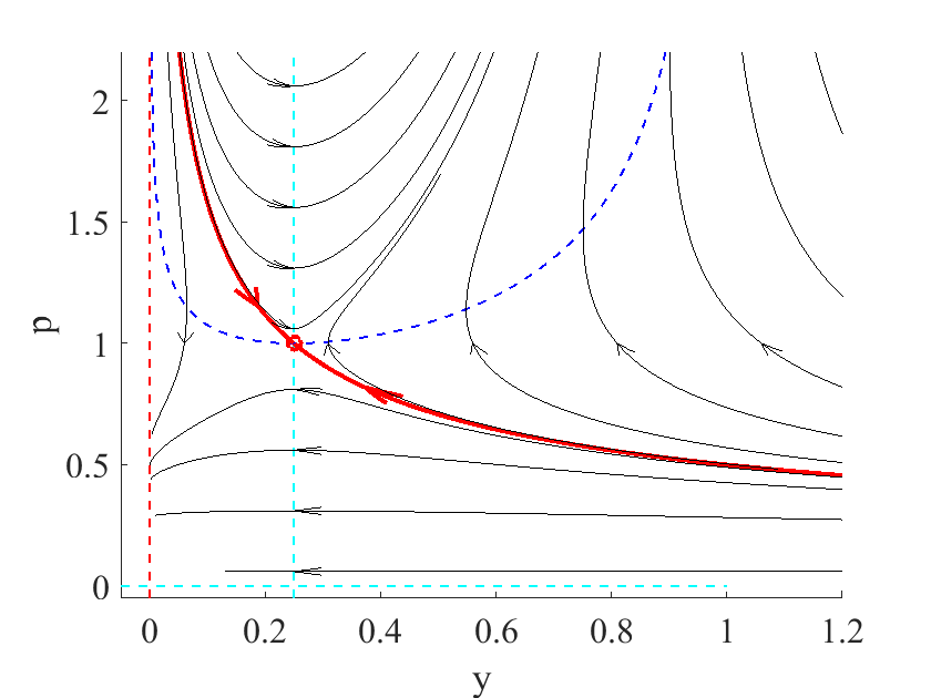
(a) $\varrho=0$.

(b) $\varrho=-1/2$.

Figure 1: The typical phase diagrams for solutions $(y(\cdot),p(\cdot))$ to (22) if (a) $\varrho>-1/2$; (b) $\varrho\leq-1/2$.

At the beginning, consider the case $\varrho>-1/2$ (see Fig. 1(a)). Since $g_{0}$ and $-g$ are strongly convex on $\mathbb{R}_{+}$, there exists a unique stationary point $(x_{0},p_{0})=((\varrho+1)^{-2}/4,(\varrho+1)/\sqrt{2\varrho+1})$ of dynamical system (21) lying in $\mathbb{R}^{2}$; furthermore, this point is a saddle point. Then, the image of the path $t\mapsto({\hat{y}}(t),{\hat{p}}(t))$, the set $\{({\hat{y}}(t),{\hat{p}}(t))\,|\,t\in\mathbb{R}\}$, is contained in the unstable manifold [26] of (22). Hence, $({\hat{y}},{\hat{p}})$ is either $\{(x_{0},p_{0})\}$ or one of two unstable paths of the system, converging to $(x_{0},p_{0})$ (see Fig. 1(a)). So, in this case, the transversality condition (11a) elicits a unique motion and for each weakly overtaking optimal process $({\hat{y}},{\hat{u}})$ with positive motion ${\hat{y}}$, its motion converges to $(\varrho+1)^{-2}/4$ as $t\uparrow\infty$.

In the case $\varrho\leq-1/2$, the system (22) has no solution $(y,p)$ with positive ${\hat{y}}(\cdot)$ (see Fig. 1(b)); therefore, in the case $\varrho\leq-1/2$ there exists no locally weakly overtaking optimal process in the optimal control problem.

Example 3.

Again consider a number $\varrho\in\mathbb{R}$ and a positive number $x_{*}$. Now take

$$g(x)\stackrel{{\scriptstyle\triangle}}{{=}}2x-x^{2},\ g_{0}(\upsilon)\stackrel{{\scriptstyle\triangle}}{{=}}-\sqrt{\upsilon}\qquad\forall x\in\mathbb{R},\upsilon\in\mathbb{R}_{+}.$$

It gives the following problem:

maximize $$\int_{0}^{\infty}e^{-{{\varrho}}\tau}\sqrt{{u(\tau)}}\,d\tau$$

subject to $$\frac{d{y}(t)}{dt}={2y(t)-y^{2}(t)}-u(t)\ \textrm{a.e.},$$

$$y(0)=x_{*}>0,\ y(t)\in\mathbb{R},\ {u(t)\in U\stackrel{{\scriptstyle\triangle}}{{=}}[0;1]},\ {\operatorname*{Limsup}_{\theta\uparrow\infty}\{\operatorname*{sign}y(\theta)\}\subset\{1\}}.$$

Note that a locally weakly overtaking optimal process $({\hat{y}},{\hat{u}})$ with positive ${\hat{y}}$ satisfies the conditions of Proposition 1. In particular, $(H1)$–$(H4)$ hold true.

Due to Proposition 1, we know that either ${\hat{u}}\equiv 1$ (with ${\hat{\lambda}}=1$, ${\hat{\psi}}={\hat{p}}=0$), or there exists sequence of solutions $(y_{n},p_{n})$ to system

$$\frac{dy(t)}{dt}=2y(t)-y^{2}(t)-\frac{1}{\max(1,4p^{2}(t))},\qquad\frac{d{p}(t)}{dt}=(\varrho-2+2y(t))p(t),$$ (23)

converging to $({\hat{y}},{\hat{p}})$ such that, for all natural $n$, one finds a positive $t$ with $y_{n}(t)=0$. So, we must seek out the solutions $({\hat{y}},{\hat{p}})$ to (23) with positive ${\hat{y}}$ such that either ${\hat{p}}\equiv 0$, or ${\hat{p}}>0$ and the sign of ${\hat{y}}$ is unstable in (23).

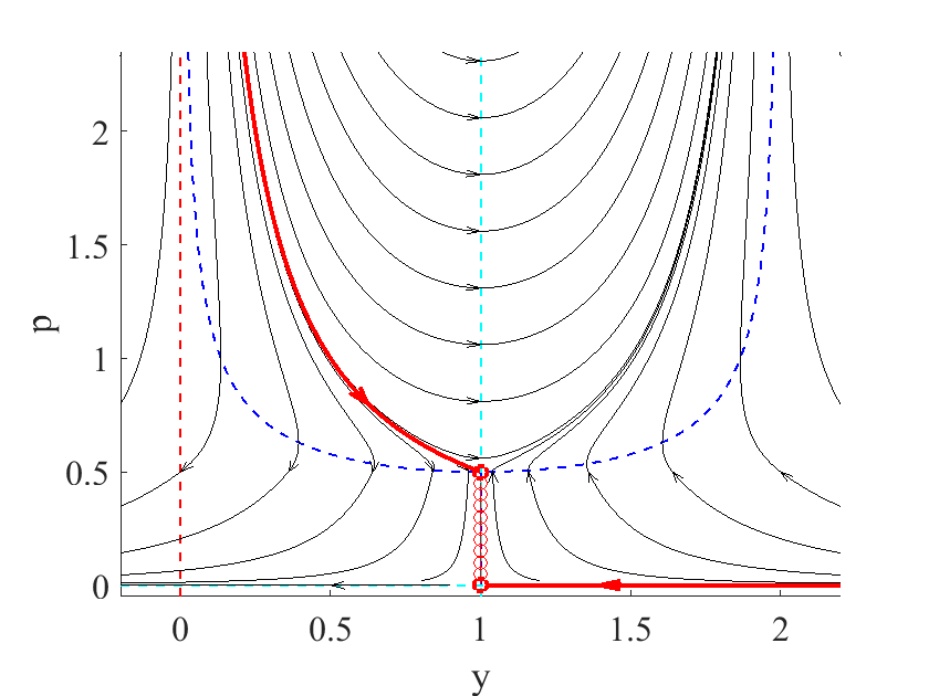
Figure 2: The phase diagram for solutions $(y(\cdot),p(\cdot))$ to (23) in the case $\varrho=0$.

At the beginning, introduce a solution $({y}^{0},0)$ to (23) with ${\hat{p}}\equiv 0$ and $y^{0}>0$. The direct calculations give ${y}^{0}(t)=\frac{(x_{*}-1)(t+1)+1}{(x_{*}-1)t+1}$ for all $t\in\mathbb{R}$; in particular, ${y}^{0}\equiv 1$ if $x_{*}=1$. Notice also that, in the case $|\varrho|<2$, $\varrho\neq 0$, there exists a positive stationary point $(x_{0},p_{0})=(1-\varrho/2;\frac{1}{\sqrt{4-\varrho^{2}}})$; furthermore, this point is unique in $(0;+\infty)\times(0;+\infty)$ and is a saddle point. Hence, there exists two unstable paths of this Hamiltonian system, converging to $(x_{0},p_{0})$ (see Fig. 3 and 4); denote these paths by $y_{\rm{left}}$ and $y_{\rm{right}}$.

In the case $\varrho=0$ (see Fig. 2) the stationary points of (23) constitute the interval $\{1\}\times[0;1/2]$ and for all $x_{*}<1$ there exists a unique path $(y_{\downarrow},p_{\downarrow})$ of (23), converging to the point $(1,1/2)$. In this case define

$$S\stackrel{{\scriptstyle\triangle}}{{=}}\{(y_{\downarrow}(t),p_{\downarrow}(t))\in\mathbb{R}_{+}\times\mathbb{R}_{+}\,|\,t\in\mathbb{R}\}\cup([1;\infty)\times\{0\})\cup(\{1\}\times[0;1/2]).$$

Later we will prove that the image of $t\mapsto({\hat{y}},{\hat{p}})$ is contained in $S$, in particular, ${\hat{y}}$ is $y_{\downarrow}$ if $x_{*}<1$ and ${y}^{0}$ otherwise.

In the case $\varrho<0$ (see Fig. 3(a,b)) there exists a unique path $(y_{\downarrow},p_{\downarrow})$ of (23), converging to the point $(1,0)$. In this case define

$$S\stackrel{{\scriptstyle\triangle}}{{=}}\{(y_{\downarrow}(t),p_{\downarrow}(t))\in\mathbb{R}_{+}\times\mathbb{R}_{+}\,|\,t\in\mathbb{R}\}\cup([1;\infty)\times\{0\}).$$

Later we will prove that the image of $t\mapsto({\hat{y}},{\hat{p}})$ is contained in $S$; in particular, ${\hat{y}}$ is $y_{\downarrow}$ if $x_{*}<1$ and ${y}^{0}$ otherwise.

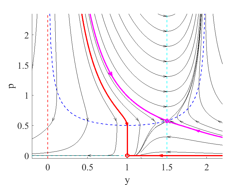
(a) $\varrho=-1$.

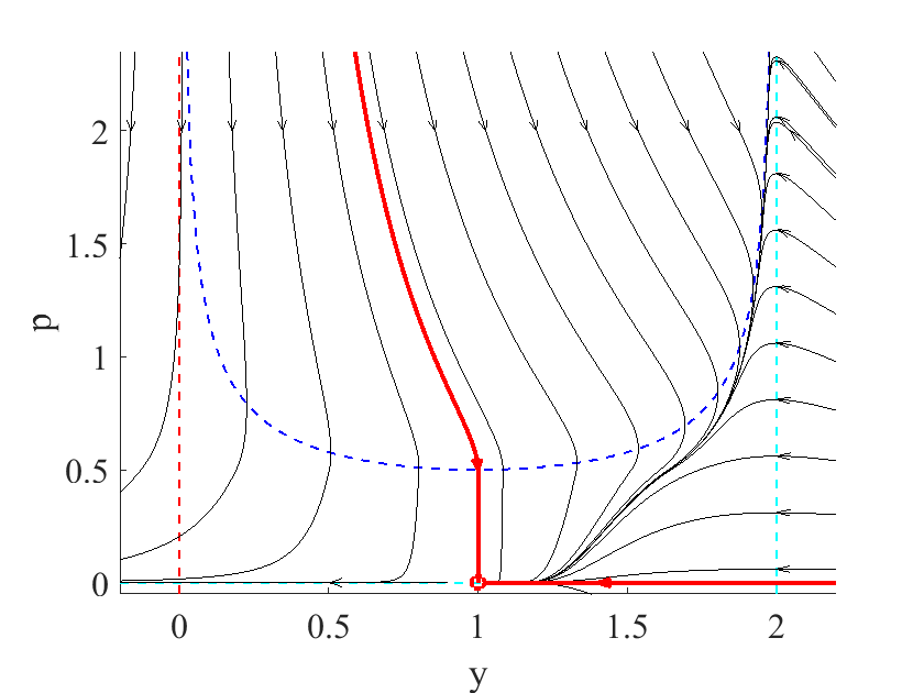
(b) $\varrho=-2$.

Figure 3: The typical phase diagrams for solutions $(y(\cdot),p(\cdot))$ to (23) if (a) $\varrho\in(-2;0)$; (b) $\varrho\leq-2$.

In the case $\varrho\in(0;2)$ (see Fig. 4(a)) the path $(y_{\rm{right}},p_{\rm{right}})$ is continuated to $-\mathbb{R}_{+}$ and its image connects $(1;0)$ and the saddle point $(x_{0},p_{0})$. In this case define

$$S\stackrel{{\scriptstyle\triangle}}{{=}} \{(y_{\rm{left}}(t),p_{\rm{left}}(t))\in\mathbb{R}_{+}\times\mathbb{R}_{+}\,|\,t\in\mathbb{R}\}\cup\{(x_{0},p_{0})\}$$

$$\cup\{(y_{\rm{right}}(t),p_{\rm{right}}(t))\in\mathbb{R}_{+}\times\mathbb{R}_{+}\,|\,t\in\mathbb{R}\}\cup([1;\infty)\times\{0\}).$$

Later we will prove that the image of $t\mapsto({\hat{y}},{\hat{p}})$ is contained in $S$, in particular, ${\hat{y}}$ is $y_{\rm{right}}$ if $x_{0}<x_{*}<1$, $y_{\rm{left}}$ if $x_{0}>x_{*}$, $x_{0}$ if $x_{0}=x_{*}$, and ${y}^{0}$ otherwise.

In the case $\varrho\geq 2$ (see Fig. 4(b)) consider the union of all images of the paths $(\check{y},\check{p})$ with positive $\check{p}$ that intersect the axe $\{0\}\times(0;+\infty)$. This set is open and connected subset of $\mathbb{R}\times(0;+\infty)$. Therefore the right boundary of this subset is the union of the images of paths. Since the stationary point $(1,0)$ is unstable and there exists no stationary point on $(0;\infty)^{2}$, this boundary is the image of a certain path $t\mapsto(y_{\uparrow},p_{\uparrow})$. So, in the case $\varrho\geq 2$ define

$$S\stackrel{{\scriptstyle\triangle}}{{=}}\{(y_{\uparrow}(t),p_{\uparrow}(t))\in\mathbb{R}_{+}\times\mathbb{R}_{+}\,|\,t\in\mathbb{R}\}\cup([1;\infty)\times\{0\}).$$

We will prove that the image of $t\mapsto({\hat{y}},{\hat{p}})$ is contained in $S$, in particular, ${\hat{y}}$ is $y_{\uparrow}$ if $x_{*}<1$ and ${y}^{0}$ otherwise.

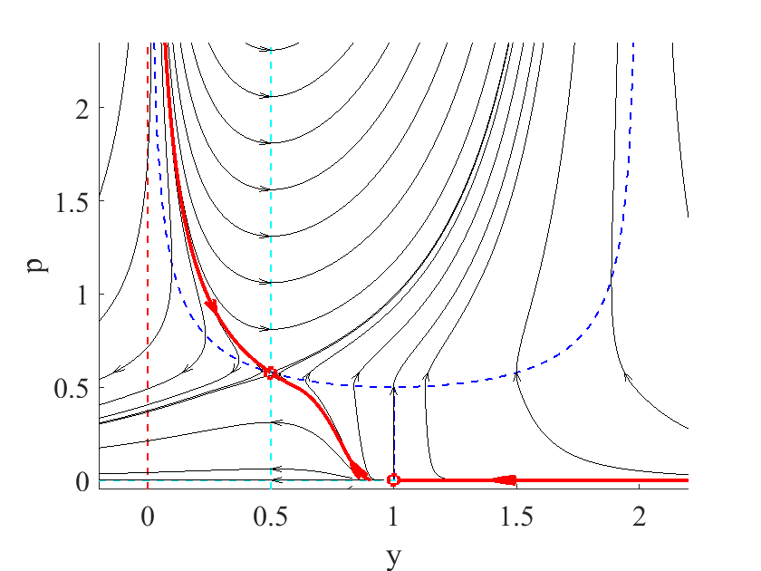
(a) $\varrho=1$.

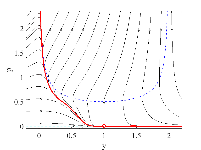
(b) $\varrho=2$.

Figure 4: The typical phase diagrams for solutions $(y(\cdot),p(\cdot))$ of (23) if (a) $\varrho\in(0;2)$; (b) $\varrho\geq 2$.

At last, we begin to prove that the image of $t\mapsto({\hat{y}}(t),{\hat{p}}(t))$ is contained in $S$ in all five cases. Indeed, on the one hand, consider any solution $(y,p)$ to (23) such that $(x_{*},p(0))$ is to the left of $S$. Then, $(y(t),p(t))$ is located to the left of $S$ for all $t$ and, for large $t$, $p(t)$ is closed to zero and $y(t)$ is negative. Since ${\hat{p}}$ must be nonnegative, $(y,p)$ can’t be $({\hat{y}},{\hat{p}})$. On the other hand, consider any solution $(y,p)$ to (23) such that $(x_{*},p(0))$ to the right of $S$. For all solutions $(\check{y},\check{p})$ near to $(y,p)$ its image is not intersects with $S$. In particular, the sign of $\check{y}$ as well as the sign of ${y}$ is positive for all positive $t$. It means that the sign of $y$ is stable. So, since $p$ is positive, $(y,p)$ can’t be $({\hat{y}},{\hat{p}})$ again. Thus, we have proved that the image of $t\mapsto({\hat{y}},{\hat{p}})$ is contained in $S$.

So, for all initial position $x_{*}>0$ and every discount rate $\varrho$ there can be at most one locally weakly overtaking optimal process, because there exists at most one solution to the Hamiltonian system satisfying the necessary conditions of Proposition 1. Since these conditions are the direct consequence of (11a), for every locally weakly overtaking optimal process to this control problem the corresponding relations (1b)-(1c) with boundary condition (11a) is a complete system of necessary conditions.

Finally, notice that for $\varrho\leq 0$ the motion ${y}^{0}$ and ${y}_{\downarrow}$ are overtaking optimal because ${\hat{u}}=1$ for all sufficiently large $t$. Besides, in the case $\varrho\in(-2;0)$ (see Fig. 3(a)) the constant motion $x_{0}$ as well as converging to $x_{0}$ motions $y_{\rm{left}}$ and $y_{\rm{right}}$ can’t be locally weakly overtaking optimal.

The remaining examples illustrate the borderline of consistent with (1c) conditions on co-state arcs in the case of the lack of asymptotic constraints. Before we proceed further, we investigate system (1a)–(1c), corresponding to both examples.

Fix a finite-dimensional real vector space $\mathbb{X}$ and a $C^{2}$-smooth function $S:\mathbb{R}\times\mathbb{X}\to\mathbb{R}$. For each positive $\theta$ and points $x_{*},\ x_{\theta}\in\mathbb{X}$, consider the following auxiliary problem:

minimize $$\int_{0}^{\theta}\Big{[}\frac{1}{4}\|u(\tau)\|^{2}+\frac{\partial S}{\partial x}\big{(}{\tau},y(\tau)\big{)}e^{-\tau}u(\tau)+\frac{\partial S}{\partial t}\big{(}{\tau},y(\tau)\big{)}\Big{]}\,d\tau$$

subject to $$\frac{d{y}(t)}{dt}=e^{-t}u(t),\ t\in[0;\theta]\ \textrm{a.e.},$$

$$y(0)=x_{*},\quad y(\theta)=x_{\theta},\quad y(t)\in\mathbb{X},\quad u(t)\in U\stackrel{{\scriptstyle\triangle}}{{=}}\mathbb{X}.$$

Consider a solution $$({\psi},{\lambda}) [0;\theta] ({y},{u})$$ (on ) to relations (1b)–(1c) corresponding to a given admissible process of this auxiliary problem. It follows from (1b) that

$$\frac{d\psi(t)}{dt}={\lambda}\frac{\partial^{2}S}{\partial x^{2}}\big{(}{t},{y}(t)\big{)}e^{-t}u(t)+{\lambda}\frac{\partial S}{\partial t\partial x}\big{(}{t},{y}(t)\big{)}={\lambda}\frac{d}{dt}\Big{(}\frac{\partial S}{\partial x}\big{(}{t},{y}(t)\big{)}\Big{)}$$

for almost all $$t\in[0;\theta] C\in\mathbb{X} {\psi}(t)=\lambda\frac{\partial S}{\partial x}(t,{y}(t))+{C} t\in[0;\theta] u(t) \frac{\lambda}{4}\|\upsilon\|^{2}+e^{-t}\big{(}\lambda\frac{\partial S}{\partial x}({t},y(t))-\psi(t)\big{)}\upsilon=\frac{\lambda}{4}\|\upsilon\|^{2}-e^{-t}C\upsilon \upsilon\in\mathbb{X} \lambda>0 \lambda=1$$. Then, one can find a satisfying for all . Because minimizes over all , we have . Then, putting , one has

$${\psi}(t)=\frac{\partial S}{\partial x}(t,{y}(t))+{C},\quad{u}(t)=2e^{-t}{C},\quad{y}(t)=x_{*}+(1-e^{-2t}){C},$$ (24a)

$$J(x_{*},0,{u};t)-S(t,y(t))+S(0,x_{*})=\frac{1-e^{-2t}}{2}||{C}||^{2}=\frac{||{y}(t)-x_{*}||^{2}}{2(1-e^{-2t})}$$ (24b)

for all $$t\in[0;\theta] J(x,0,{u};t)-S(t,\mathrm{y}(x,0,{u},t))+S(0,x) x\in\mathbb{X}$$. In particular, since is independent of , we also have

$$\frac{\partial J}{\partial x}(y(0),0,{u};t)=\frac{\partial S}{\partial x}(t,y(t))-\frac{\partial S}{\partial x}(0,x_{*})=\psi(t)-\psi(0)\qquad\forall t\in[0;\theta].$$ (24c)

Note also that no co-state arc satisfies relations (1b)–(1c) with $${\lambda}=0$$.

Having all required formulae, let us finish considering this auxiliary problem and return to examples of infinite-horizon control problems.

The following example will show that condition (13a) might fail if the gradient of the limit of ${\hat{J}}$ does not coincide with the limit of gradients of ${\hat{J}}$ at $x_{*}$ (cf. (14)).

Example 4.

Assume that the function $\mathbb{X}\ni x\mapsto\limsup_{\theta\uparrow\infty}S(\theta,x)$ attains its minimum at the point $x_{*}=0$.

Then, the admissible control process $({\hat{y}},{\hat{u}})=(0,0)$ is weakly overtaking optimal in the problem

minimize $$\int_{0}^{\infty}\Big{[}\frac{1}{4}\|u(\tau)\|^{2}+\frac{\partial S}{\partial x}\big{(}{\tau},y(\tau)\big{)}e^{-\tau}u(\tau)+\frac{\partial S}{\partial t}\big{(}{\tau},y(\tau)\big{)}\Big{]}\,d\tau$$

subject to $$\frac{d{y}(t)}{dt}=e^{-t}u(t)\ \textrm{a.e.},$$

$$y(0)=0,\ y(t)\in\mathbb{X},\ u(t)\in U=\mathbb{X}.$$

Hence there exists a co-state arc ${\hat{\psi}}\in C(\mathbb{R}_{+},\mathbb{X}^{*})$ satisfying the corresponding to $({\hat{y}},{\hat{u}})$ relations (1b)-(1c) with ${\hat{\lambda}}=1$; moreover, (24a) holds for a certain ${\hat{C}}$. It follows from ${\hat{u}}\equiv 0$ that ${\hat{C}}=0$ and ${\hat{\psi}}(t)=\frac{\partial S}{\partial x}(t,0)$ for all positive $t\geq 0$.

Consider the transversality condition (13a). By $\frac{\partial{\hat{J}}}{\partial x}(0;\theta)=\psi(\theta)-\psi(0)$, the co-state arc ${\hat{\psi}}$ satisfies this condition iff the co-state arc ${\hat{\psi}}(\theta)=\frac{\partial S}{\partial x}(\theta,0)$ converges to zero as $\theta\uparrow\infty$. Note that, in this example, condition (13a) is equivalent to Shell’s condition [44, 41]: $\psi(\theta)\to 0$. By comparison, $\frac{\partial S}{\partial x}(\theta,0)=0$ holds for all $\theta$ large enough iff the Arrow-like condition [43, 41] holds: $\displaystyle\limsup\nolimits_{\theta\uparrow\infty}{\hat{\psi}}(\theta)({\hat{y}}(\theta)-{y}(\theta))\geq 0$ for all admissible control processes $(y,u)$.

So, in Example 4, the corresponding to a weakly overtaking optimal process $({\hat{y}},{\hat{u}})=(0,0)$ relations (1b)–(1c) have a solution satisfying the transversality condition (13a) iff the function $S$ satisfies the following additional asymptotic assumption: the gradients $\frac{\partial S}{\partial x}(\theta,0)$ converge to zero as $\theta\uparrow\infty.$ For instance, this is false if we take

$$\mathbb{X}\stackrel{{\scriptstyle\triangle}}{{=}}\mathbb{R},\qquad\mathbb{R}_{+}\times\mathbb{R}\ni(t,x)\mapsto S(t,x)\stackrel{{\scriptstyle\triangle}}{{=}}e^{-t}\sin(e^{t}x)-e^{-x^{2}}.$$

In this case, the cost functional $J$ and all its derivatives are bounded for all control processes. In particular, there could not be $\lambda=0$, i.e., all solutions to the Pontryagin Maximum Principle are not abnormal whenever $x_{*}$. Furthermore, the corresponding infinite-horizon problem has the unique overtaking optimal process (moreover, a unique strongly optimal [17], a unique classical optimal [13], and a unique (O)-optimal [48] process), this process has a unique (up to a positive factor) solution to (1a)–(1c), and the corresponding transversality condition (13a) is well defined; after all, this condition is not consistent with (1c). Thus, the necessity of (13a) depends primarily on the asymptotics of $\frac{\partial{\hat{J}}}{\partial x}$ rather than the qualitative properties of system (1a)–(1c).

The dynamics and the integrand in the last example are linear in $x$, whilst the functions $S$ and $\frac{\partial S}{\partial x}$ are periodic. It is enough that for a given $x_{*}$ in the corresponding infinite-horizon control problem the dimension of the set of optimal processes coincides with $\dim\mathbb{X}$. By this reason, their co-state arcs at $t=0$ also form a ball in $\mathbb{X}^{*}$. Inclusion (11a) as a unified necessary transversality condition has to take this into account.

Example 5.

Put $\mathbb{X}\stackrel{{\scriptstyle\triangle}}{{=}}\mathbb{R}^{2}$. Define the map $S$ as follows:

$$\mathbb{R}_{+}\times\mathbb{R}^{2}\ni(t,x_{1},x_{2})\mapsto S(t,x_{1},x_{2})\stackrel{{\scriptstyle\triangle}}{{=}}{x}_{1}\sin(t)-{x}_{2}\cos(t).$$

Then, the corresponding infinite-horizon control problem is

minimize $$\int_{0}^{\infty}\Big{[}\frac{\|u(\tau)\|^{2}}{4}+(e^{-\tau}{u}_{1}(\tau)+{y}_{2}(\tau))\sin(\tau)$$

$$\qquad\qquad\qquad\qquad+({y}_{1}(\tau)-e^{-\tau}{u}_{2}(\tau))\cos(\tau)\Big{]}\,d\tau$$

subject to $$\frac{d{y_{1}}(t)}{dt}=e^{-t}u_{1}(t),\frac{d{y_{2}}(t)}{dt}=e^{-t}u_{2}(t)\ \textrm{a.e.\ }t\geq 0,$$

$$(y_{1},y_{2})(0)=x_{*},\ (y_{1},y_{2})(t)\in\mathbb{R}^{2},\ (u_{1},u_{2})(t)\in U=\mathbb{R}^{2}.$$

Consider a weakly overtaking optimal process $({\hat{y}},{\hat{u}})$ in this problem. Note that $(H0)$–$(H6)$ are fulfilled. By Theorem 1, there exists a nonzero solution $({\hat{\psi}},{\hat{\lambda}})$ to system (1b)–(1c) and (11b), corresponding to this process. Note that for each positive $\theta$, this pair is also the solution to this system for the auxiliary control problem with $x_{\theta}={\hat{y}}(\theta).$ Then, first, ${\hat{\lambda}}$ is positive, and one can take ${\hat{\lambda}}=1$; second, by (24a), one find a ${\hat{C}}\in\mathbb{X}^{*}$ satisfying ${\hat{\psi}}(t)=\frac{\partial S}{\partial x}(t,{\hat{y}}(t))+{\hat{C}}$ for all nonnegative $t$. Hence, by (24c), condition (11b) is equivalent to

$$-\frac{\partial S}{\partial x}(0,x_{*})-{\hat{C}}=-{\hat{\psi}}(0)\in\operatorname*{co}\big{\{}(\sin\theta,-\cos\theta)\,\big{|}\,\theta\in[0;2\pi]\big{\}}-\frac{\partial S}{\partial x}(0,x_{*}),$$

i.e., $||{\hat{C}}||\leq 1$. Thus, according to (11b), every weakly overtaking optimal process satisfies (24a) with some ${\hat{C}}$, $||{\hat{C}}||\leq 1$.

We claim that each process with this property is a weakly overtaking optimal. Fix an admissible process $(\bar{y},\bar{u})$ satisfying (24a) for some $\bar{C}$, $||\bar{C}||\leq 1$. Consider another admissible control process $(y,u)$. By (24b), the function $J(x_{*},0,\bar{u};\theta)-S(\theta,\bar{y}(\theta))+S(0,x_{*})$ converges to $||\bar{C}||^{2}/2$ as $\theta\uparrow\infty$. Then, it is necessary to find a $\phi\in[0;2\pi]$ satisfying

$$\limsup_{n\to\infty}\big{[}J(x_{*},0,u;\phi+2\pi n)-S(\phi,x_{*}+\bar{C})+S(0,x_{*})-{||\bar{C}||^{2}}/{2}\big{]}\geq 0.$$

Note that $J(x_{*},0,u;\theta)$ tends to infinity as $\theta\uparrow\infty$ if the total variation of $y$ is unbounded. Therefore, one can assume that the motion $y$ converges to a $x_{*}+C_{\infty}\in\mathbb{X}$ as $t\to\infty$. For every positive $\theta$, there exists an admissible control process $(y_{\theta},u_{\theta})$ optimal in the auxiliary problem with $x_{\theta}=y_{\theta}(\theta)$; in particular, $J(x_{*},0,u;\theta)\geq J(x_{*},0,u_{\theta};\theta)$. Hence, by (24b), it follows from $y_{\theta}(\theta)\to C_{\infty}$ that one has

$$\limsup_{n\to\infty}J(x_{*},0,u;\phi+2\pi n)\geq S(\phi,x_{*}+C_{\infty})-S(0,x_{*})+{||C_{\infty}||^{2}}/{2}.$$

Then, we must find a $\phi\in[0;2\pi]$ so that the number

$$S(\phi,x_{*}+C_{\infty})-S(\phi,x_{*}+\bar{C})+\frac{||C_{\infty}||^{2}-||\bar{C}||^{2}}{2}=S(\phi,C_{\infty}-\bar{C})+\frac{||C_{\infty}||^{2}-||\bar{C}||^{2}}{2}$$

is nonnegative. Note that for each vector $z\in\mathbb{X}$, one finds a $\phi\in[0;2\pi]$ such that $S(\phi,z)=||z||$. Therefore, it is required to prove only $2||x-\bar{C}||\geq||\bar{C}||^{2}-||x||^{2}=\big{(}\|\bar{C}\|-\|x\|\big{)}\big{(}\|\bar{C}\|+\|x\|\big{)}$ for all vectors $x=C_{\infty}\in\mathbb{R}^{2}$. The latter is evident at all $x$ where $||x||+||\bar{C}||\leq 2$, while at vectors $x$ where $||x||>2-||\bar{C}||$ it follows from $||\bar{C}||^{2}\leq 1\leq(2-||\bar{C}||)^{2}<||x||^{2}$ because of $||\bar{C}||\leq 1$.

Thus, it is shown that every admissible control process satisfying (24a) with some $\bar{C}$, $||\bar{C}||\leq 1$, is weakly overtaking optimal. Then, each co-state arc satisfying (11a) generates the unique weakly overtaking optimal process and each weakly overtaking optimal process possesses its own co-state arc satisfying (11a).

Summing up, for every weakly overtaking optimal process in this example, there exists a unique co-state arc satisfying (1c). Therefore, each necessary condition on co-state arcs must either satisfy each of them or distinguish them. Due to the linearity of the dynamics and integrand in $x$, any necessary condition depending only on a co-state arc is satisfied for all such co-state arcs. In this example, all such co-state arcs $\psi$ satisfy $||\psi(0)+(0,1)||\leq 1$. Since inclusion (11a) also points to the same set, in this example this inclusion becomes the tightest of all boundary conditions on the co-state arcs consistent with (1c).

6 Subdiffentials of lower and upper limits of scalar functions

Let a family of maps ${W}_{\theta}$, $\theta\geq 0$, from a finite-dimensional space $\mathbb{X}$ to $\mathbb{R}\cup\{+\infty\}$ be given. Define the maps $W_{\inf}$ and $W_{\sup}$ from $\mathbb{X}$ to $\mathbb{R}\cup\{-\infty,+\infty\}$ by the rules

$$W_{\inf}(x)\stackrel{{\scriptstyle\triangle}}{{=}}\liminf_{\theta\uparrow\infty}{W}_{\theta}(x),\qquad W_{\sup}(x)\stackrel{{\scriptstyle\triangle}}{{=}}\limsup_{\theta\uparrow\infty}{W}_{\theta}(x)\qquad\forall x\in\mathbb{X}.$$ (25)

For every nonempty subset ${{\mathcal{X}}}$ of a finite-dimensional space $\mathbb{X}$, define the maps $\mathop{{\mathcal{X}}\textrm{-inf}}W$ and $\mathop{{{\mathcal{X}}}\textrm{-sup}}W$ from $\mathbb{X}$ to $\mathbb{R}\cup\{-\infty,+\infty\}$ as follows:

$$(\mathop{{\mathcal{X}}\textrm{-inf}}W)(\check{x})\stackrel{{\scriptstyle\triangle}}{{=}}\liminf_{\begin{subarray}{c}\theta\uparrow\infty,\\ {{\mathcal{X}}}\ni x\to\check{x}\end{subarray}}{W}_{\theta}(x),\quad(\mathop{{\mathcal{X}}\textrm{-sup}}W)(\check{x})\stackrel{{\scriptstyle\triangle}}{{=}}\operatorname*{lsc}\limsup_{\begin{subarray}{c}\theta\uparrow\infty,\\ {{\mathcal{X}}}\ni x\to\check{x}\end{subarray}}{W}_{\theta}(x)$$ (26)

if $\check{x}\in\operatorname*{cl}{{\mathcal{X}}}$ and $+\infty$ otherwise. Note that both maps are lower semicontinuous.

First, consider subdifferentials of the lower epigraphical limit of $W_{\theta}$.

Following [40, Sect. 7.3], for every sequence of $g_{n}:{\mathbb{X}}\to\mathbb{R}\cup\{-\infty,+\infty\}$, denote by $\displaystyle\operatorname*{e-liminf}_{n\uparrow\infty}g_{n}$ and $\displaystyle\operatorname*{e-limsup}_{n\uparrow\infty}g_{n}$ the epigraphical lower and upper limits of $g_{n}$: for all $x\in\mathbb{X}$

$$\operatorname*{e-liminf}_{n\uparrow\infty}g_{n}(x) \stackrel{{\scriptstyle\triangle}}{{=}}\lim_{\varkappa\downarrow 0}\liminf_{n\uparrow\infty}\inf_{||x-z||\leq\varkappa}g_{n}(z)\in\mathbb{R}\cup\{-\infty,+\infty\},$$

$$\operatorname*{e-limsup}_{n\uparrow\infty}g_{n}(x) \stackrel{{\scriptstyle\triangle}}{{=}}\lim_{\varkappa\downarrow 0}\limsup_{n\uparrow\infty}\inf_{||x-z||\leq\varkappa}g_{n}(z)\in\mathbb{R}\cup\{-\infty,+\infty\}.$$

When these two functions coincide, we say that the functions $g_{n}$ epi-converge to

$$\operatorname*{e-lim}_{n\uparrow\infty}g_{n}\stackrel{{\scriptstyle\triangle}}{{=}}\operatorname*{e-liminf}_{n\uparrow\infty}g_{n}=\operatorname*{e-limsup}_{n\uparrow\infty}g_{n}.$$

Note that the epigraphical lower and upper limits is lower semicontinuous [40, Proposition 7.4(a)].

The first lemma is the consequence of the corresponding results of [21].

Lemma 1.

Let for a given neighborhood ${G}\subset\mathbb{X}$ maps ${W}_{\theta}:\mathbb{X}\to\mathbb{R}$ be lower semicontinuous on $G$ for all positive $\theta$. Assume that

$$\operatorname*{e-liminf}_{\theta\uparrow\infty}W_{\theta}(z)=W_{\inf}(z)\qquad\forall z\in{G}.$$ (27)

Then, for all $\check{z}\in{G}$ satisfying $|W_{\inf}(\check{z})|<+\infty$, one has

$${\partial}W_{\inf}(\check{z})\subset\bigcap_{\begin{subarray}{c}(\theta_{n})_{n\in\mathbb{N}}\in\mathbb{R}_{+}^{\mathbb{N}},\ \theta_{n}\uparrow\infty,\\ \operatorname*{dist}(\check{z},W_{\inf}(\check{z});\operatorname*{gph}W_{\theta_{n}})\to 0\end{subarray}}\operatorname*{Limsup}_{\begin{subarray}{c}n\uparrow\infty,\ z\to\check{z},\\ |W_{\theta_{n}}(z)-W_{\theta_{n}}(\check{z})|\to 0\end{subarray}}{\hat{\partial}}W_{\theta_{n}}(z),$$ (28)

i.e., for every limiting subgradient $\xi\in{\partial}W_{\inf}(\check{z})$ and every unbounded increasing sequence of positive numbers $\theta_{n}\in\mathbb{R}_{+}$ satisfying $\operatorname*{dist}(\check{z},W_{\inf}(\check{z});\operatorname*{gph}W_{\theta_{n}})\to 0$ there exist sequences of points $z_{n}\in\mathbb{X}$ and gradients $\zeta_{n}\in{\hat{\partial}}W_{\theta_{n}}(z_{n})$ satisfying $\|z_{n}-\check{z}\|\to 0$, $\|\zeta_{n}-\check{z}\|\to 0$, and $|W_{\theta_{n}}(z_{n})-W_{\theta_{n}}(\check{z})|\to 0$ as $n\uparrow\infty$.

Proof Consider a point $\check{z}\in{G}$.

Let $\mathcal{T}(\check{z})$ be the set of all unbounded increasing sequences of positive $\theta_{n}$ such that one has $\operatorname*{dist}(\check{z},W_{\inf}(\check{z});\operatorname*{gph}W_{\theta_{n}})\to 0$ and the sequence of maps

$$\mathbb{X}\ni z\mapsto\ W_{\theta_{n}}(z)$$ (29)

epi-converges. Fix such a sequence of $\theta_{n}$, consider the corresponding epi-limit

$$\mathbb{X}\ni z\mapsto\widetilde{W}_{\{\theta_{n}\}}(z)\stackrel{{\scriptstyle\triangle}}{{=}}\operatorname*{e-lim}_{n\uparrow\infty}W_{\theta_{n}}(z);$$ (30)

this function is lower semicontinuous by [40, Proposition 7.4(a)].

Fix a subgradient $\xi\in{\hat{\partial}}W_{\inf}(\check{z})$. By [35, Theorem 1.27], since $\mathbb{X}$ is finite-dimensional, there exist a $C^{1}$-smooth function $g:\mathbb{X}\to\mathbb{R}$ and a neighbourhood $G^{\prime}\subset G$ of the point $\check{z}$ such that one has $\xi=\frac{\partial g}{\partial z}(\check{z})$, ${W}_{\inf}(\check{z})=g(\check{z})$, and $\operatorname*{lsc}{W}_{\inf}(z)-\operatorname*{lsc}{W}_{\inf}(\check{z})\geq g(z)-g(\check{z})$ for all $z\in G^{\prime}$.

Now, on the one hand, (27) entails $\widetilde{W}_{\{\theta_{n}\}}({z})\geq W_{\inf}({z})$ for all $z\in G$; on the other hand, $\operatorname*{dist}(\check{z},W_{\inf}(\check{z});\operatorname*{gph}W_{\theta_{n}})\to 0$ leads to $\widetilde{W}_{\{\theta_{n}\}}(\check{z})\leq W_{\inf}(\check{z})$. Then, one has $\widetilde{W}_{\{\theta_{n}\}}(\check{z})=W_{\inf}(\check{z})=g(\check{z})$ and $\widetilde{W}_{\{\theta_{n}\}}(z)-\widetilde{W}_{\{\theta_{n}\}}(\check{z})\geq g(z)-g(\check{z})$ for all $z\in G^{\prime}$. By [35, Theorem 1.27], $\xi=\frac{\partial g}{\partial z}(\check{z})$ lies in ${\hat{\partial}}\widetilde{W}_{\{\theta_{n}\}}(\check{z})$.

Recall that the sequence of functions $W_{\theta_{n}}$ is asymptotically locally equicoercive [19, Definition 4.4] if for a bounded sequence of $x_{k}\in\mathbb{X}$, from

$$\sup_{k\in\mathbb{N}}W_{\theta_{n(k)}}(x_{k})<+\infty$$

for a given unbounded sequence of $n(k)$, it follows that there exists a converging subsequence of the sequence of $x_{k}.$ Then, the sequence of $W_{\theta_{n}}$ has this property, since $\mathbb{X}$ is finite-dimensional. According to [21, Proposition 2.2(v) and Theorem 5.3(ii)], it follows that

$$\xi\in{\hat{\partial}}\widetilde{W}_{\{\theta_{n}\}}(\bar{z})\subset\operatorname*{Limsup}_{{z\to\bar{z},\ n\uparrow\infty,\ W_{\theta_{n}}(z)\to\widetilde{W}_{\{\theta_{n}\}}(\check{z})}}{\hat{\partial}}{W}_{\theta_{n}}(z)\qquad\forall\bar{z}\in{G}$$

holds for all sequences $(\theta_{n})_{n\in\mathbb{N}}\in\mathcal{T}(\check{z})$ because of the epigraphical convergence of (29) to $\widetilde{W}_{\{\theta_{n}\}}$. Hence, the convergence $W_{\theta_{n}}(\check{z})\to\widetilde{W}_{\{\theta_{n}\}}(\check{z})={W}_{\inf}(\check{z})$ with $\xi\in{\hat{\partial}}\widetilde{W}_{\{\theta_{n}\}}(\check{z})$ gives

$$\xi\in\bigcap_{(\theta_{n})_{n\in\mathbb{N}}\in\mathcal{T}(\check{z})}\operatorname*{Limsup}_{\begin{subarray}{c}n\uparrow\infty,\ z\to\check{z},\\ |W_{\theta_{n}}(z)-W_{\inf}(\check{z})|\to 0\end{subarray}}{\hat{\partial}}{W}_{\theta_{n}}(z).$$ (31)

Since the right side of this inclusion is upper semicontinuous, we obtain that (31) holds true for all $\xi\in{\partial}W_{\inf}(\check{z})$.

To prove (28), suppose to the contrary that one can find a positive $\varepsilon$ and an unbounded increasing sequence of positive $\theta_{n}$ satisfying

$$\operatorname*{dist}(\check{z},W_{\inf}(\check{z});\operatorname*{gph}W_{\theta_{n}})\to 0$$

such that one has $|W_{\theta_{n}}({z}_{n})-W_{\inf}(\check{z})|+||\zeta_{n}-\xi||+||z_{n}-\check{z}||>\varepsilon$ for all sequences of points $z_{n}\in{G}$ and gradients $\zeta_{n}\in{\hat{\partial}}{W}_{\theta_{n}}(z_{n})$. Then, the sequence of $\theta_{n}$ (and every its subsequence) would not satisfy (31). Hence the sequence of maps (29) would not have any epi-converging subsequence. However, since $W_{\inf}(\check{z})$ is finite, the sequence of ${W}_{\theta_{n}}$ does not escape epigraphically to the horizon, and, by [40, Theorem 7.6], possesses an epi-converging subsequence. We get a contradiction.

Thus, Lemma 1 has been proved. $\Box$

Lemma 2.

Let $C$ be a nonempty subset of $\mathbb{X}$. Let maps ${W}_{\theta}:\mathbb{X}\to\mathbb{R}$ be $1$-Lipschitz continuous on $\mathbb{X}$.

Then, for all $\check{z}\in C$ satisfying $|(\mathop{{C}\textrm{-inf}}W)(\check{z})|<+\infty$, one has

$${\partial}(\mathop{{C}\textrm{-inf}}W)(\check{z})\subset N(\check{z};\operatorname*{cl}C)+\bigcap_{\begin{subarray}{c}(\theta_{n})_{n\in\mathbb{N}}\in\mathbb{R}_{+}^{\mathbb{N}},\ \theta_{n}\uparrow\infty,\\ |(\mathop{{C}\textrm{-inf}}W)({z})-W_{\theta_{n}}(z)|\to 0\end{subarray}}\operatorname*{Limsup}_{\begin{subarray}{c}n\uparrow\infty,\ z\to\check{z},\\ |W_{\theta_{n}}(z)-W_{\theta_{n}}(\check{z})|\to 0\end{subarray}}{\hat{\partial}}W_{\theta_{n}}(z).$$ (32)

Proof

First, note that 1-Lipschitz continuity of all the $W_{\theta}$ as well as $W_{\inf}(z)$ yields that

$$\operatorname*{lsc}(W_{\theta}+{\imath}_{C})=W_{\theta}+\operatorname*{lsc}{\imath}_{C}=W_{\theta}+{\imath}_{\operatorname*{cl}C},\quad\operatorname*{lsc}(W_{\inf}+{\imath}_{C})=W_{\inf}+{\imath}_{\operatorname*{cl}C}.$$

In particular, for all $z\in{\operatorname*{cl}C}$ one has

$$(\mathop{{C}\textrm{-inf}}W)({z})=\operatorname*{e-liminf}_{\theta\uparrow\infty}(W_{\theta}(z)+{\imath}_{C})(z)=W_{\inf}(z)+{\imath}_{\operatorname*{cl}C}(z).$$ (33)

Furthermore, $\operatorname*{dist}(z,(\mathop{{C}\textrm{-inf}}W)({z});\operatorname*{gph}(W_{\theta_{n}+\imath_{C}}))\to 0$ iff $|(\mathop{{C}\textrm{-inf}}W)({z})-(W_{\theta_{n}}+\imath_{C}))(z)|\to 0$ iff $|(\mathop{{C}\textrm{-inf}}W)({z})-W_{\theta_{n}}(z)|\to 0$ for all $z\in C$.

Second, for all positive $\theta$, the fuzzy sum rule [14, Theorem 3.3.3] leads to

$${\hat{\partial}}(W_{\theta}+{\imath}_{\operatorname*{cl}C})({z})\subset\operatorname*{Limsup}_{\operatorname*{cl}C\ni{\hat{z}}\to{z}}{\hat{N}}({\hat{z}};\operatorname*{cl}C)+\operatorname*{Limsup}_{{\hat{z}}\to{z}}{\hat{\partial}}W_{\theta}({\hat{z}})\qquad\forall{z}\in\operatorname*{cl}C.$$

Furthermore, by [35, Theorem 1.6] we also have

$${\hat{\partial}}(W_{\theta}+{\imath}_{\operatorname*{cl}C})({z})\subset N({z};\operatorname*{cl}C)+\operatorname*{Limsup}_{\begin{subarray}{c}{\hat{z}}\to{z},\\ |W_{\theta}({\hat{z}})-W_{\theta}({z})|\to 0\end{subarray}}\check{\partial}W_{\theta}({\hat{z}})\qquad\forall{z}\in\operatorname*{cl}{C}.$$ (34)

At last, note that (33) is condition (27) with $W_{\theta}+{\imath}_{\operatorname*{cl}C}$ instead of $W_{\theta}$. Now, for all every $\check{z}\in C$, inclusion (28) with $W_{\theta}+{\imath}_{\operatorname*{cl}C}$ instead of $W_{\theta}$ is

$${\partial}(\mathop{{C}\textrm{-inf}}W)(\check{z}) \subset\bigcap_{\begin{subarray}{c}(\theta_{n})_{n\in\mathbb{N}}\in\mathbb{R}_{+}^{\mathbb{N}},\ \theta_{n}\uparrow\infty,\\ |(\mathop{{C}\textrm{-inf}}W)({z})-W_{\theta_{n}}(z)|\to 0\end{subarray}}\operatorname*{Limsup}_{\begin{subarray}{c}n\uparrow\infty,C\ni z\to\check{z},\\ |W_{\theta_{n}}(z)-W_{\theta_{n}}(\check{z})|\to 0\end{subarray}}{\hat{\partial}}(W_{\theta}+{\imath}_{\operatorname*{cl}C})(z).$$

Applying (34), we obtain (32). Lemma 2 has been proved. $\Box$

In [33, Theorem 6.1(i)], the following upper-estimate of Fréchet subdifferentials of the upper epigraphical limit of lower semicontinuous functions $W_{\theta}$ was shown:

$${\hat{\partial}}\Big{(}\operatorname*{e-limsup}\nolimits_{\theta\uparrow\infty}W_{\theta}\Big{)}(\check{z}) \subset\operatorname*{co}\operatorname*{Limsup}_{\theta\uparrow\infty,z\to\check{z}}{\hat{\partial}}{W}_{\theta}(z)$$

$$=\bigcap_{\varkappa>0}\operatorname*{co}\operatorname*{cl}\bigcup_{\theta>1/\varkappa,\ {z\in\mathbb{X},\ ||z-\check{z}||<\varkappa}}{\hat{\partial}}{W}_{\theta}(z)\qquad\forall\check{z}\in\mathbb{X}.$$

Repeating the proof of the previous Lemma word-for-word and using this inclusion instead to (28), we obtain the following result.

Lemma 3.

Let $C$ be a nonempty subset of $\mathbb{X}$. Let maps ${W}_{\theta}:\mathbb{X}\to\mathbb{R}$ be $1$-Lipschitz continuous on $\mathbb{X}$.

Then, for all $\check{z}\in C$ satisfying $|(\mathop{{C}\textrm{-sup}}W)(\check{z})|<+\infty$, one has

$${\partial}\big{(}\mathop{{C}\textrm{-sup}}W\big{)}(\check{z})\subset\operatorname*{co}N(\check{z};\operatorname*{cl}C)+\operatorname*{co}\operatorname*{Limsup}_{\theta\uparrow\infty,z\to\check{z}}{\hat{\partial}}{W}_{\theta}(z).$$ (35)

The following lemma is the keystone of this section.

Lemma 4.

Let a family of nonempty closed subsets $\Omega_{\theta}\subset\mathbb{X}$, $\theta>0$, be given. Consider also the closed sets $\Omega_{\inf}$ and $\Omega_{\sup}$ defined as follows:

$$\Omega_{\inf}\stackrel{{\scriptstyle\triangle}}{{=}}\operatorname*{Liminf}_{\theta\uparrow\infty}\Omega_{\theta}=\operatorname*{cl}\bigcup_{\theta>0}\bigcap_{\theta^{\prime}>\theta}\Omega_{\theta^{\prime}},\qquad\Omega_{\sup}\stackrel{{\scriptstyle\triangle}}{{=}}\operatorname*{Limsup}_{\theta\uparrow\infty}\Omega_{\theta}=\bigcap_{\theta>0}\operatorname*{cl}\bigcup_{\theta^{\prime}>\theta}\Omega_{\theta^{\prime}}.$$

Then, for every subset $C\subset\mathbb{X}$ and point $\check{z}\in C$

$${N}(\check{z};\Omega_{\sup}\cap C) \subset{N}(\check{z};\operatorname*{cl}C)+\bigcap_{\begin{subarray}{c}(\theta_{n})_{n\in\mathbb{N}}\in\mathbb{R}_{+}^{\mathbb{N}},\;\theta_{n}\uparrow\infty,\\ \operatorname*{dist}(\check{z};\Omega_{\theta_{n}})\to 0\end{subarray}}\operatorname*{Limsup}_{{n\uparrow\infty,\;z\to\check{z}}}{\hat{N}}({z};\Omega_{\theta})\ \textrm{if}\ \check{z}\in\Omega_{\sup};$$ (36)

$${N}(\check{z};\Omega_{\inf}\cap C) \subset\operatorname*{co}{N}(\check{z};\operatorname*{cl}C)+\operatorname*{co}\operatorname*{Limsup}_{{z\to\check{z},\theta\uparrow\infty}}{\hat{N}}({z};\Omega_{\theta})\ \textrm{if}\ \check{z}\in\Omega_{\inf}.$$ (37)

Proof Define $W_{\theta}\stackrel{{\scriptstyle\triangle}}{{=}}\operatorname*{dist}(\cdot;\Omega_{\theta})$ for all positive $\theta$. For all $z\in\mathbb{X}$ these functions satisfy the following equalities:

$$\operatorname*{dist}(z;\Omega_{\inf}\cap C)=\operatorname*{e-limsup}_{\theta\uparrow\infty}\operatorname*{dist}(z;\Omega_{\theta}\cap C)=(\mathop{{C}\textrm{-sup}}W)(z),$$

$$\operatorname*{dist}(z;\Omega_{\sup}\cap C)=\operatorname*{e-liminf}_{\theta\uparrow\infty}\operatorname*{dist}(z;\Omega_{\theta}\cap C)=(\mathop{{C}\textrm{-inf}}W)(z).$$

Now, from (32) and (35) it follows that

$${\partial}\operatorname*{dist}(\check{z};\Omega_{\inf}\cap C) \subset N(\check{z};\operatorname*{cl}C)+\bigcap_{\begin{subarray}{c}(\theta_{n})_{n\in\mathbb{N}}\in\mathbb{R}_{+}^{\mathbb{N}},\ \theta_{n}\uparrow\infty,\\ \operatorname*{dist}(\check{z};\Omega_{\theta_{n}})\to 0\end{subarray}}\operatorname*{Limsup}_{\begin{subarray}{c}n\uparrow\infty,\\ z\to\check{z}\end{subarray}}{\hat{\partial}}{W}_{\theta_{n}}(z)\quad\forall\check{z}\in\Omega_{\inf};$$ (38)

$${\partial}\operatorname*{dist}(\check{z};\Omega_{\sup}\cap C) \subset\operatorname*{co}N(x;\operatorname*{cl}C)+\operatorname*{co}\operatorname*{Limsup}_{\theta\uparrow\infty,z\to\check{z}}{\hat{\partial}}{W}_{\theta}(z)\qquad\forall\check{z}\in\Omega_{\sup}.$$ (39)

Now, (36) and (37) follow from equalities (9).

The key lemma has been proved. $\Box$

The next two lemmata do not follow from similar results in [33, 36, 38].

Lemma 5.

Let maps ${W}_{\theta}:\mathbb{X}\to\mathbb{R}\cup\{-\infty,+\infty\}$ be lower semicontinuous for all positive $\theta$. Given a subset ${{\mathcal{X}}}\subset\mathbb{X}$, a point $\check{z}\stackrel{{\scriptstyle\triangle}}{{=}}(\check{x},\check{y})\in\operatorname*{epi}(\mathop{{\mathcal{X}}\textrm{-inf}}W)$, and a normal $(\zeta,-\lambda)$ in ${N}(\check{z};\operatorname*{epi}(\mathop{{\mathcal{X}}\textrm{-inf}}W))$. Assume also that $\check{y}=W_{\theta}(\check{x})$ for all positive $\theta$.

Then:

• (i)

  $$(\zeta,-\lambda)\in{N}(\check{x};\operatorname*{cl}\mathcal{X})\times\{0\}+\bigcap_{{(\theta_{n})_{n\in\mathbb{N}}\in\mathbb{R}_{+}^{\mathbb{N}},\theta_{n}\uparrow\infty}}\operatorname*{Limsup}_{n\uparrow\infty,\ z\to\check{z}}{\hat{N}}({z};\operatorname*{epi}W_{\theta_{n}}).$$ (40a)

• (ii) Furthermore,

  $$\zeta\in{N}(\check{x};\operatorname*{cl}\mathcal{X})+\bigcap_{{(\theta_{n})_{n\in\mathbb{N}}\in\mathbb{R}_{+}^{\mathbb{N}},\theta_{n}\uparrow\infty}}\operatorname*{Limsup}_{\begin{subarray}{c}n\uparrow\infty,\;x\to\check{x},\;\lambda^{\prime}\downarrow\lambda,\\ W_{\theta}(x)\to\check{y}\end{subarray}}\lambda^{\prime}{\hat{\partial}}W_{\theta_{n}}(x)$$ (40b)

  if all the $W_{\theta}$ are Lipschitz continuous on a given neighbourhood $G$ of $\check{x}$.

Proof

Fix a subset ${{\mathcal{X}}}\subset\mathbb{X}$ and a point $\check{z}\stackrel{{\scriptstyle\triangle}}{{=}}(\check{x},\check{y})\in\operatorname*{epi}(\mathop{{\mathcal{X}}\textrm{-inf}}W)$. Note that from $\check{z}\stackrel{{\scriptstyle\triangle}}{{=}}(\check{x},\check{y})\in\operatorname*{epi}(\mathop{{\mathcal{X}}\textrm{-inf}}W)$ it follows that $\check{x}\in\operatorname*{cl}\mathcal{X}$.

Put $C\stackrel{{\scriptstyle\triangle}}{{=}}\mathcal{X}\times\mathbb{R}$ and $\Omega_{\theta}\stackrel{{\scriptstyle\triangle}}{{=}}\operatorname*{epi}W_{\theta}$ for every positive $\theta$. Then, $\Omega_{\sup}\cap C=\operatorname*{epi}(\mathop{{\mathcal{X}}\textrm{-inf}}W)$. Now, by Lemma 4, for every point $\check{z}\stackrel{{\scriptstyle\triangle}}{{=}}(\check{x},\check{y})\in\operatorname*{epi}(\mathop{{\mathcal{X}}\textrm{-inf}}W)$, inclusion (36) holds. Hence, every normal $(\zeta,-\lambda)$ in ${N}(\check{z};\operatorname*{epi}(\mathop{{\mathcal{X}}\textrm{-inf}}W))$ satisfies (40a). So, (40a) has been proved.

To prove (40b), note that the cone ${\hat{N}}(x,g(x);\operatorname*{epi}g)$ of a Lipschitz continuous function $g$ is $\cup_{r\geq 0}r({\hat{\partial}}g(x)\times\{-1\})$. Also ${\hat{N}}(z;\operatorname*{epi}g)$ is contained in $\{0\}$ if the point $z$ does not lie in the graph of $g$. Hence, we may rewrite the inclusion (40a) as

$$(\zeta,-\lambda)\in{N}(\check{x};\operatorname*{cl}\mathcal{X})\times\{0\}+\bigcap_{\begin{subarray}{c}(\theta_{n})_{n\in\mathbb{N}}\in\mathbb{R}_{+}^{\mathbb{N}},\\ \theta_{n}\uparrow\infty\end{subarray}}\operatorname*{Limsup}_{\begin{subarray}{c}n\uparrow\infty,\;x\to\check{x},\;\lambda^{\prime}>0,\\ W_{\theta}(x)\to\check{y}\end{subarray}}\lambda^{\prime}({\hat{\partial}}W_{\theta_{n}}(x)\times\{-1\}).$$

Hence a sequence of $\lambda^{\prime}_{n}$ has to converge to $\lambda$ and (40b) has been proved. $\Box$

Lemma 6.

Let maps ${W}_{\theta}:\mathbb{X}\to\mathbb{R}\cup\{-\infty,+\infty\}$ be lower semicontinuous for all positive $\theta$. Given a subset ${{\mathcal{X}}}\subset\mathbb{X}$, a point $\check{z}\stackrel{{\scriptstyle\triangle}}{{=}}(\check{x},\check{y})\in\operatorname*{epi}(\mathop{{\mathcal{X}}\textrm{-sup}}W)$, and a normal $(\zeta,-\lambda)$ in ${N}(\check{z};\operatorname*{epi}(\mathop{{\mathcal{X}}\textrm{-sup}}W))$.

Then:

• (i)

  $$(\zeta,-\lambda)\in\operatorname*{co}{N}(\check{x};\operatorname*{cl}\mathcal{X})\times\{0\}+\operatorname*{co}\operatorname*{Limsup}_{{z\to\check{z},\ \theta\uparrow\infty}}{\hat{N}}({z};\operatorname*{epi}W_{\theta}).$$ (41a)

• (ii) Furthermore,

  $$\zeta\in\operatorname*{co}{N}(\check{x};\operatorname*{cl}\mathcal{X})+\operatorname*{co}\operatorname*{Limsup}_{\begin{subarray}{c}\theta\uparrow\infty,\ x\to\check{x},\ \lambda^{\prime}\to\lambda,\\ W_{\theta}(x)\to\check{y}\end{subarray}}\lambda^{\prime}{\hat{\partial}}W_{\theta}(x)$$ (41b)

  if all the $W_{\theta}$ are Lipschitz continuous on a given neighbourhood $G$ of $\check{x}$.

• (iii)

  $$\zeta\in{N}(\check{x};\operatorname*{cl}\mathcal{X})+\lambda\operatorname*{co}\operatorname*{Limsup}_{\begin{subarray}{c}\theta\uparrow\infty,\ x\to\check{x},\\ W_{\theta}(x)\to\check{y}\end{subarray}}{\hat{\partial}}W_{\theta}(x)$$ (41c)

  if there exists a neighbourhood $G$ of $\check{x}$ and a positive $R$ such that all the $W_{\theta}$ are $R$-Lipschitz continuous on ${G}$.

Proof

The proof of (41a) and (41b) follows from (37) as well (40a) and (40b) from (36).

To prove (41c), note that in the case of $R$-Lipschitz continuity of all the $W_{\theta}|_{G}$, the functions $\operatorname*{lsc}W_{\theta}|_{G}=W_{\theta}|_{G}$ and $W_{\sup}|_{G}=\big{(}\mathop{{\mathcal{X}}\textrm{-sup}}W\big{)}|_{G}$ have the same property. It follows that $\mathop{{\mathcal{X}}\textrm{-sup}}W$ coincides with ${\imath}_{\operatorname*{cl}\mathcal{X}}+W_{\sup}$ on $G$. In addition, since every singular limiting subgradient of Lipschitz continuous function $W_{\sup}|_{G}$ is zero, the subdifferential qualification condition [35, (2.34)] for $W_{\sup}$ and ${\imath}_{\operatorname*{cl}\mathcal{X}}$ is applied. Now, by [35, (2.35) and (2.36)] we obtain that

$$\partial^{\infty}(W_{\sup}+{\imath}_{\operatorname*{cl}\mathcal{C}})|_{G}=\partial^{\infty}{\imath}_{\operatorname*{cl}\mathcal{C}}|_{G}=N(\cdot;\operatorname*{cl}\mathcal{C})|_{G},\ \partial(W_{\sup}+{\imath}_{\operatorname*{cl}\mathcal{C}})|_{G}=\partial W_{\sup}|_{G}.$$

It means that

$$N(\check{x};\operatorname*{epi}(\mathop{{\mathcal{X}}\textrm{-sup}}W))\!=\!N(\check{x};\operatorname*{epi}({\imath}_{\operatorname*{cl}\mathcal{X}}+W_{\sup}))\!=\!N(\check{x};\operatorname*{cl}{\mathcal{X}})\times\{0\}+N(\check{x},\check{y};\operatorname*{epi}W_{\sup}).$$

Applying (41a) for the function $W_{\sup}|_{G}=(\mathop{{G}\textrm{-sup}}W)|_{G}$ and using the boundedness of the norms of all Fréchet subdifferentials of $W_{\theta}|_{G}$, we obtain

$$(\zeta,-\lambda)\in N(\check{x};\operatorname*{cl}{\mathcal{X}})\times\{0\}+\lambda\operatorname*{co}\operatorname*{Limsup}_{\begin{subarray}{c}x\to\check{x},\ \theta\uparrow\infty\\ W_{\theta}({x})\to\check{y}\end{subarray}}{\hat{\partial}}W_{\theta}({x})\times\{-1\}$$

for all normal $(\zeta,-\lambda)$ in ${N}(\check{z};\operatorname*{epi}(\mathop{{\mathcal{X}}\textrm{-sup}}W))$. So, (41c) has verified.

The final lemma has been proved. $\Box$

7 Proofs of Theorems 1 and 2

We will prove both theorems simultaneously. The idea of the proof is briefly described as follows. At the beginning, following Halkin’s method [25] and ideas of [18, Section 25.2], we will reduce the verification of all desired relations on $\mathbb{R}$ with set $U$ to its verification on finite intervals $[0;n]$ with each finite subset $\Upsilon_{n}(t)$ of $U$. Then, for fixed $n$, extending $f$ and $f_{0}$ from $[0;n]$ to $[0;2n]$ by back-track, we will consider a new dynamics function $\bar{f}_{n}$ and integrand $\bar{f}_{0,n}$; this trick ensures the transfer of the right endpoint to ${\hat{y}}(0)$. Next, we will rewrite the corresponding criteria (the weakly overtaking criterion in Theorem 1 and the overtaking criterion in Theorem 2) in terms of a constrained optimisation problem in a finite-dimensional space. Further, we will reduce this problem to some finite-horizon control problem. Proceeding to Halkin’s method, we will consider the corresponding Pontryagin Maximum Principle [18, Theorem 22.26] for this control problem and estimate the happened transversality condition by Lemma 6 and Lemma 5 in the proof of Theorem 1 and the proof of Theorem 2, respectively.

Step 1.

Let $\Upsilon$ be a finite subset of $\mathcal{U}$. For all natural $n$ and nonnegative $t$ define the sets

$$U_{n}(t)\stackrel{{\scriptstyle\triangle}}{{=}}\big{\{}\upsilon\in U\,\big{|}\, \|f(t,{\hat{y}}(t),\upsilon)-f(t,{\hat{y}}(t),{\hat{u}}(t))\|\ \$$

$$\ +|f_{0}(t,{\hat{y}}(t),\upsilon)|+L_{\upsilon}(t)+L_{{\hat{u}}(t)}(t)\leq n\big{\}},$$

$$\Upsilon_{n}(t)\stackrel{{\scriptstyle\triangle}}{{=}}\big{\{}u(t)\,\big{|}\, u\in\Upsilon,u(t)\in U_{n}(t)\big{\}}\cup\{{\hat{u}}(t)\}$$

for all nonnegative $t$. In particular, ${\hat{u}}(t)$ lies in $\Upsilon_{n}(t)$ whenever $t$ and $n$.

Denote by $\mathfrak{Q}_{\diamond}$ the set of all pair $({\lambda},{\psi})\in[0;1]\times C(\mathbb{R}_{+},\mathbb{X}^{*})$ satisfying with $({\hat{y}},{\hat{u}})$ the equality $\|\psi(0)\|+\lambda=1$, adjoint equation (1b), condition (10), and the corresponding condition among (11a)–(11c) (in the proof of Theorem 1) or among (12a)-(12b) (in the proof of Theorem 2). One verifies easily that this set is closed. Then, $\mathfrak{Q}_{\diamond}$ is compact.

Consider the the following assertion:

• $(A)$ for each finite subset $\Upsilon$ of $\mathcal{U}$ and each natural $n$ there exist a nonzero pair $({\lambda}_{n},{\psi}_{n})\in\{0,1\}\times C([0;n],\mathbb{X}^{*})$ satisfying

  • the inequality

    $${H}\big{(}{\hat{y}}(t),{\psi}_{n}(t),\upsilon,\lambda_{n},t\big{)}\!\leq\!{H}\big{(}{\hat{y}}(t),{\psi}_{n}(t),{\hat{u}}(t),\lambda_{n},t\big{)}$$ (42)

    for all $\upsilon\in\Upsilon_{n}(t)$ and almost all $t\in[0;n]$,

  • as well as adjoint equation (1b) with $({\hat{y}},{\hat{u}})$,

  • transversality condition (10),

  • and the corresponding condition among (11a)–(11c) (in the proof of Theorem 1) or among (12a)-(12b) (in the proof of Theorem 2).

In the next two steps we will show that both theorems are implied from the assertion $(A)$.

Step 2.

Assume that assertion $(A)$ is established for all finite subsets $\Upsilon$ of $\mathcal{U}$ and all natural $n$.

Fix a such $\Upsilon$. Denote by $\mathfrak{Q}_{\diamond}^{\Upsilon}$ the set of all pair $({\lambda},{\psi})\in\mathfrak{Q}_{\diamond}$ satisfying inequality (42) for almost all nonnegative $t$ for each $\upsilon\in\Upsilon$.

We claim that from $(A)$ it follows that $\mathfrak{Q}_{\diamond}^{\Upsilon}$ is nonempty and closed.

To prove this, applying the assertion $(A)$ for all natural $n$, consider the corresponding sequence of $({\lambda}_{n},{\psi}_{n})$.

Scaling each $\psi_{n}$, if necessary, one can also suppose that ${\psi}_{n}(0)=n$ if $\lambda_{n}=0$. Then, passing from the sequence of $n$ to its subsequence, if necessary, one can assume that either all $\lambda_{n_{k}}$ equal to $1$ and the sequence of $\psi_{n_{k}}(0)$ converges to a vector $\phi_{0}\in\mathbb{X}^{*}$, or the sequence of $||\psi_{n_{k}}(0)||$ is unboundedly increasing and the sequence of $\psi_{n_{k}}(0)/||\psi_{n_{k}}(0)||$ converges to a nonzero vector $\phi_{0}\in\mathbb{X}^{*}$. Put ${\hat{\lambda}}\stackrel{{\scriptstyle\triangle}}{{=}}1$ and $r_{k}\stackrel{{\scriptstyle\triangle}}{{=}}1$ if $\lambda_{n_{k}}\equiv 1$ and put ${\hat{\lambda}}\stackrel{{\scriptstyle\triangle}}{{=}}0$ and $r_{k}\stackrel{{\scriptstyle\triangle}}{{=}}1/||\psi_{n_{k}}(0)||$ otherwise. In both cases, the sequence of $(r_{k}\psi_{n_{k}}(0),r_{k}\lambda_{n_{k}})$ converges to $(\phi_{0},{\hat{\lambda}})$.

Now, each pair $(r_{k}\psi_{n_{k}}(0),r_{k}\lambda_{n_{k}})$ satisfies (1b) and inherits all transversality conditions that are verified for $({\psi}_{n_{k}},{\lambda}_{n_{k}})$. Further, by the theorem on continuous dependence of solutions to differential equations on the initial state, the sequence of $r_{k}\psi_{n_{k}}$ converges on $\mathbb{R}_{+}$ to the solution ${\hat{\psi}}$ to (1b) with ${\hat{\psi}}(0)=\phi_{0}$ and $\lambda={\hat{\lambda}}$. Note that this convergence is uniform on an arbitrary compact interval. Hence the pair $({\hat{\psi}},{\hat{\lambda}})$ also satisfies (1b) on the whole $\mathbb{R}_{+}$. Moreover, it follows that this pair satisfies inequality (42) for almost all nonnegative $t$ for each $u\in\Upsilon$.

So, there exists a nonzero pair $({\hat{\lambda}},{\hat{\psi}})\in\{0,1\}\times C(\mathbb{R}_{+},\mathbb{X}^{*})$ satisfying adjoint equation, desired transversality conditions, and inequality (42) for almost all nonnegative $t$ for all $\upsilon\in\Upsilon$. Then, the pair $(\lambda_{\diamond},\psi_{\diamond})\stackrel{{\scriptstyle\triangle}}{{=}}\frac{1}{{\hat{\lambda}}+\|{\hat{\psi}}(0)\|}({\hat{\lambda}},{\hat{\psi}})$ lies in $\mathfrak{Q}_{\diamond}^{\Upsilon}$.

For any converging sequence of $(\lambda^{n}_{\diamond},\psi^{n}_{\diamond})\in\mathfrak{Q}_{\diamond}^{\Upsilon}$ define $r_{n}=1$ if $\lambda^{n}_{\diamond}=0$ and $r_{n}=1/\lambda^{n}_{\diamond}$ otherwise. Repeating the previous three paragraphs literally with the sequence of $({\lambda}_{n},{\psi}_{n})\stackrel{{\scriptstyle\triangle}}{{=}}r_{n}(\lambda^{n}_{\diamond},\psi^{n}_{\diamond})$, we obtain that the limit of $(\lambda^{n}_{\diamond},\psi^{n}_{\diamond})$ also lies in $\mathfrak{Q}_{\diamond}^{\Upsilon}$.

Thus, $\mathfrak{Q}_{\diamond}^{\Upsilon}$ is a nonempty and closed subset of $\mathfrak{Q}_{\diamond}$ for each finite subset $\Upsilon$ of $\mathcal{U}$.

Step 3.

Now we show that the both theorems are implied from $(A)$.

Indeed, for each finite subset $\Upsilon$ of $\mathcal{U}$, the nonempty set $\mathfrak{Q}_{\diamond}^{\Upsilon}$ is closed in the compact $\mathfrak{Q}_{\diamond}$. By the finite intersection property, there exists a pair $(\lambda_{\diamond},\psi_{\diamond})$ lies in $\mathfrak{Q}_{\diamond}^{\Upsilon}$ for all finite subsets $\Upsilon$.

We will prove that $(\lambda_{\diamond},\psi_{\diamond})$ satisfies (1c). Suppose to the contrary that one can find a subset of positive measure in which (1c) fails. Then, for all $n$ large enough, consider the sets

$$V_{n}(t)\stackrel{{\scriptstyle\triangle}}{{=}}\big{\{}\upsilon\in U\,\big{|}\,{H}\big{(}{\hat{y}}(t),{\psi}_{\diamond}(t),\upsilon,\lambda_{\diamond},t\big{)}-{H}\big{(}{\hat{y}}(t),{\psi}_{\diamond}(t),{\hat{u}}(t),\lambda_{\diamond},t\big{)}>1/n\big{\}}$$

are nonempty on a subset of positive measure. Increasing $n$ if necessary, we can guarantee that the set

$$\check{U}_{n}(t)\stackrel{{\scriptstyle\triangle}}{{=}}U_{n}(t)\cap V_{n}(t)$$

is nonempty on a subset $\mathcal{T}$ of positive measure. Since the graph of $\check{U}_{n}$ is measurable, Aumann’s selection theorem [7] yields the existence of a measurable function $\check{u}$ having values in $\check{U}_{n}(t)$ for almost all $t\in\mathcal{T}$. Define $\check{u}(t)={\hat{u}}(t)$ for all $t\notin\mathcal{T}$. Then, it follows that (42) with $\upsilon=\check{u}(t)$ fails for $t$ from the set of positive measure, therefore $(\lambda_{\diamond},\psi_{\diamond})$ does not lies in $\mathfrak{Q}_{\diamond}^{\Upsilon}$ if $\Upsilon=\{\check{u}\}$. We get the contradiction.

So, $(\lambda_{\diamond},\psi_{\diamond})$ satisfies (1c). Dividing $(\lambda_{\diamond},\psi_{\diamond})$ by $\lambda_{\diamond}$ if $\lambda_{\diamond}\notin\{0,1\}$, we obtain the desired pair $({\hat{\lambda}},{\hat{\psi}})$ with ${\hat{\lambda}}\in\{0,1\}$.

Thus, it is required to prove only assertion $(A)$ for each natural $n$ and each finite subset $\Upsilon$ of $\mathcal{U}$.

Step 4.

Fix a finite subset $\Upsilon\subset\mathcal{U}$ and natural $n$ with the corresponding set-valued map $\Upsilon_{n}:\mathbb{R}\rightrightarrows U$. For all positive $\alpha\leq n$ denote by $\mathcal{U}_{\alpha}$ the set of all Lebesgue measurable functions $u:\mathbb{R}_{+}\to U$ satisfying ${u}|_{[n;\infty)}={\hat{u}}|_{[n;\infty)}$,

$$\operatorname*{meas}\{\tau\in[0;n]\mid u(\tau)\neq{\hat{u}}(\tau)\}\leq\alpha,\ \textrm{and}\ u(t)\in\Upsilon_{n}(t)\ \textrm{for almost all}\ t\in[0;n].$$

Denote by $\mathbb{X}_{\alpha}$ the closed $\alpha$-ball centered in ${\hat{y}}(0)$. At last, take $\beta(n)$ from (4) in the definition of the corresponding (locally weakly overtaking and locally overtaking) criterion.

Introduce $L_{\Upsilon}(t)\stackrel{{\scriptstyle\triangle}}{{=}}\sup_{\upsilon\in\Upsilon_{n}(t)}L_{\upsilon}(t)$ for all $t\in[0;n]$. Define $M\stackrel{{\scriptstyle\triangle}}{{=}}e^{\int_{0}^{n}L_{\Upsilon}(\tau)\,d\tau}$. It is finite by $(H2)$ and $(H3)$.

Consider the neighborhood of $\operatorname*{gph}{\hat{y}}$, the set $\mathbb{G}_{\Upsilon}=\cap_{\upsilon\in\Upsilon}\mathbb{G}_{\upsilon}\cap{\hat{\mathbb{G}}}$ (see $(H2)$ and $(H3)$). Decreasing ${\hat{\mathbb{G}}}$ if necessary, we may get that $\mathbb{G}_{\Upsilon}\cap([0;n]\times\mathbb{X})$ is bounded. If $(H5)$ holds, decreasing again, we may get that the set $\{(t,x)\in\mathbb{G}_{\Upsilon}\mid t=0\}$ is contained in $\{0\}\times\mathbb{G}_{\exists}$. Similarly, if $(H6)$ is also fulfilled, this set may be contained in $\{0\}\times\mathbb{G}_{\partial}$.

Note that, by $(H2)$ and $(H3)$, for all $u\in\mathcal{U}_{n}$ the maps $(t,x)\mapsto f(t,x,u(t))$ and $(t,x)\mapsto f_{0}(t,x,u(t))$ are Lipschitz continuous on $\mathbb{G}_{\Upsilon}$ of rank $L_{\Upsilon}(t)$. Applying the inequality $\|f(t,x,u)\|\leq\|f(t,{\hat{y}}(t),{\hat{u}}(t))\|+\|f(t,{\hat{y}}(t),u)-f(t,{\hat{y}}(t),{\hat{u}}(t))\|+L_{\Upsilon}(t)\|x-{\hat{y}}(t)\|$, we obtain that the norms of these maps on $\mathbb{G}_{\Upsilon}$ are also bounded by the locally summable function $n+\|f(t,{\hat{y}}(t),{\hat{u}}(t))\|+|f_{0}(t,{\hat{y}}(t),{\hat{u}}(t))|+RL_{\Upsilon}(t)$, here $R$ is the diameter of $\mathbb{G}_{\Upsilon}\cap([0;n]\times\mathbb{X})$. Now, for every $u\in\mathcal{U}_{n}$ the maps $\mathrm{y}(x,t,\upsilon;\cdot)$ and $J(x,t,\upsilon;\cdot)$ are well-defined and continuous on an interval if $(t,x)\in{\mathbb{G}}_{\upsilon}$; furthermore, for every positive $\theta$ the map $x\mapsto J(x,0,{\hat{u}};\theta)={\hat{J}}(x;\theta)$ is continuous around ${\hat{y}}(0)$ and, by $(H4)$, is strictly differentiable at this point.

Further, decreasing the neighborhood $\mathbb{G}_{\Upsilon}$ if necessary, on can suppose that the set all the graphs of $\mathrm{y}(x,t,{\hat{u}};\cdot)|_{[0;n]}$, $(t,x)\in\mathbb{G}_{\Upsilon}$, are containing in $\mathbb{G}_{\Upsilon}$, i.e., this set is strongly invariant with respect to $(t,x)\mapsto f(t,x,{\hat{u}}(t)).$ In addition, there exists a positive $\gamma\leq\min({\beta}(n)/2,1)/2M^{2}n$ such that, the closed $2Mn\gamma$-ball centered in $(t,{\hat{y}}(t))$ belongs to $\mathbb{G}_{\Upsilon}$ for all $t\in[0;n]$. Now, all graphs of $\mathrm{y}(x,0,{\hat{u}};\cdot)|_{[0;n]}$ (with $x\in\mathbb{X}_{\gamma}$) are contained in $\mathbb{G}_{\Upsilon}$.

At last, since ${f}$ and ${f}_{0}$ on ${G}_{\Upsilon}$ is Lipschitz continuous in $x$ of rank $L_{\Upsilon}(t)$, by definitions of $\mathbb{G}_{\Upsilon}$, and $M$, the inequality

$$\||x_{1}-x_{2}||\leq M\|\mathrm{y}(x_{1},t,{\hat{u}};0)-\mathrm{y}(x_{2},t,{\hat{u}};0)\|$$ (43)

holds for all $t\in[0;n]$, $(t,x_{1}),(t,x_{2})\in\mathbb{G}_{\Upsilon}$.

Step 5.

Define the dynamics $\bar{f}_{n}:[0;2n]\times\mathbb{X}\times U\to\mathbb{X}$ and the integrand $\bar{f}_{0,n}:[0;2n]\times\mathbb{X}\times U\to\mathbb{R}$ as follows: for all $(t,x,u)\in[0;2n]\times{\mathbb{X}}\times U$,

$$(\bar{f}_{n},\bar{f}_{0,n})(t,x,u)=\left\{\begin{array}[]{cc}(f,f_{0})(t,x,u)&\textrm{if}\ t<n;\\ -(f,f_{0})(2n-t,x,{\hat{u}}(2n-t))&\textrm{if}\ t\geq n.\end{array}\right.$$

Put

$$\widetilde{G}\stackrel{{\scriptstyle\triangle}}{{=}}\bigcup_{(t,x,s)\in\mathbb{G}_{\Upsilon}\times\mathbb{R}}\big{\{}(t,x,s),(2n-t,x,s)\big{\}}.$$

Note that since one has $\widetilde{G}\cap([0;n]\times\mathbb{X}\times\mathbb{R})\subset\mathbb{G}_{\Upsilon}$ and $(\bar{f}_{n},\bar{f}_{0,n})(2n-t,x,u(t))=-(\bar{f}_{n},\bar{f}_{0,n})(t,x,u(t))$, the function $(\bar{f}_{n},\bar{f}_{0,n})$ on $\widetilde{G}$ inherits the properties $f$ and $f_{0}$ on $\mathbb{G}_{\Upsilon}$. In particular, the vector fields $(\bar{f}_{n},\bar{f}_{0,n})(t,\cdot,u)$, $u\in\Upsilon_{n}(t)$, are locally Lipschitz continuous in $x$ on $\widetilde{G}$ and its norms are bounded by a summable function of time.

Fix a control $u\in\mathcal{U}_{\gamma}$ and $x\in\mathbb{X}$ with $(0,x)\in\mathbb{G}_{\Upsilon}$. Denote by $(\bar{\mathrm{y}}_{n},\bar{\mathrm{w}}_{n})(x,u;\cdot)$ a solution to

$$\frac{d\bar{y}(\tau)}{d\tau}=\bar{f}_{n}(\tau,\bar{y}(\tau),u(\tau)),\ \frac{d\bar{w}(\tau)}{d\tau}=\bar{f}_{0,n}(\tau,\bar{y}(\tau),u(\tau))$$ (44)

with the initial condition $(\bar{y},\bar{w})(0)=(x,0)$ on the maximum existing interval $I_{u,x}\subset[0;2n]$. Notice that this solution is unique if

$$\operatorname*{gph}(\bar{\mathrm{y}}_{n},\bar{\mathrm{w}}_{n})(x,u;\cdot)|_{I_{u,x}}\subset\widetilde{G}.$$ (45)

Now, we will prove that $I_{u,x}=[0;2n]$, (4), and (45) hold if either $u\equiv{\hat{u}}$ or $x\in\mathbb{X}_{\gamma}$.

Step 6.

In the case $u={\hat{u}}$, $x\in\mathbb{G}_{\Upsilon}$, by the construction of $\mathbb{G}_{\Upsilon}$ and the definition $\bar{f}$, the solution $(\bar{\mathrm{y}}_{n},\bar{\mathrm{w}}_{n})(x,{\hat{u}};\cdot)$ exists and this solution is unique on $[0;n]$. Since $(\bar{f}_{n},\bar{f}_{0,n})$ and $\widetilde{G}$ are symmetric in $t$, each solution $(\bar{y}_{n},\bar{w}_{n})|_{[0;n]}$ to (44) has the unique continuation on $[0;2n]$ by the rule:

$$(\bar{y}_{n},\bar{w}_{n})(2n-t)=(\bar{y}_{n},\bar{w}_{n})(t)\quad\forall t\in[0;n].$$

In particular, the motion

$${\hat{\bar{y}}}_{n}(t)\stackrel{{\scriptstyle\triangle}}{{=}}\bar{\mathrm{y}}\big{(}{\hat{y}}(0),{\hat{u}};t\big{)},\ {\hat{\bar{w}}}_{n}(t)\stackrel{{\scriptstyle\triangle}}{{=}}\bar{\mathrm{w}}\big{(}{\hat{y}}(0),{\hat{u}};t\big{)}\qquad\forall t\in[0;2n]$$

satisfies ${\hat{\bar{y}}}_{n}(2n)={\hat{\bar{y}}}_{n}(0)={\hat{y}}(0)$ and ${\hat{\bar{w}}}_{n}(2n)={\hat{\bar{w}}}_{n}(0)=0.$

Consider a $u\in\mathcal{U}_{\gamma}$, $x\in\mathbb{X}_{\gamma}$ with its solution $(\bar{\mathrm{y}}_{n},\bar{\mathrm{w}}_{n})(x,u;\cdot)$ on the maximal interval $I_{u,x}$. This solution exists and is unique at least until the exit $\bar{\mathrm{y}}_{n}(x,u;\cdot)$ from the bounded set $\widetilde{G}_{\Upsilon}\cap([0;n]\times\mathbb{R}^{n})$. Note also that, since $\mathbb{G}_{\Upsilon}$ is strongly invariant with respect to the generated by ${\hat{u}}$ dynamics, for every $t\in[0;n]$ we get $(t,(\bar{\mathrm{y}}_{n},\bar{\mathrm{w}}_{n})(x,u;t))\in\widetilde{G}$ in the case of $(0,\mathrm{y}(\bar{\mathrm{y}}_{n}(x,u;t),t,{\hat{u}};0),0)\in\mathbb{G}_{\Upsilon}$. The following instance

$$\tau_{u,x}\stackrel{{\scriptstyle\triangle}}{{=}}\min\{t\in[0;n]\mid\|\mathrm{y}(\bar{\mathrm{y}}_{n}(x,u;t),t,{\hat{u}};0)-{\hat{y}}(0)\|=2nM\gamma\}\cup\{n\}$$

lies in $I_{u,x}$ because the closed $2nM\gamma$-ball centered in ${\hat{y}}(t)$ belongs to $\mathbb{G}_{\Upsilon}$. We claim that $\tau_{u,x}=n$, $[0;n]\subset I_{u,x}$ hold true, and $y(\cdot)\stackrel{{\scriptstyle\triangle}}{{=}}\bar{\mathrm{y}}_{n}(x,u;\cdot)|_{I_{u,x}}$ satisfies (4); in addition, the corresponding pair $(y(\cdot)|_{[0;n]},u(\cdot))$ is a control process on $[0;n]$.

Indeed, note that $(t,y(t))\in\mathbb{G}_{\Upsilon}$ and $\|\mathrm{y}(y(t),t,{\hat{u}};0)-{\hat{y}}(0)\|\leq 2nM\gamma$ hold for all $t\in[0;\tau_{u,x}]$ by the definition of $\tau_{u,x}$. Now, by (43) and $x\in\mathbb{X}_{\gamma}$, the inequality $\|\mathrm{y}(y(t),t,{\hat{u}};t)-{\hat{y}}(t)\|\leq M\|\mathrm{y}(y(t),t,{\hat{u}};0)-{\hat{y}}(0)\|\leq 2nM^{2}\gamma<1$ also holds. From the definition of $U_{n}(t)$, it follows

$$\Big{\|}\frac{d}{dt}(y(\tau)-\mathrm{y}(y(t),t,{\hat{u}};\tau))\big{|}_{\tau=t}\Big{\|}=\|{f}(t,y(t),u(t))-{f}(t,{y}(t),{\hat{u}}(t))\|$$

$$\leq(L_{u(t)}(t)+L_{{\hat{u}}(t)}(t))\|y(t)-{\hat{y}}(t)\|+\|{f}(t,y(t),u(t))-{f}(t,{\hat{y}}(t),u(t))\|$$

$$<(L_{u(t)}(t)+L_{{\hat{u}}(t)}(t))2nM^{2}\gamma+\|{f}(t,y(t),u(t))-{f}(t,{\hat{y}}(t),u(t))\|<n$$

and $\frac{d}{dt}(\mathrm{y}(y(t),t,{\hat{u}};0)-{\hat{y}}(0))\leq Mn$. Now, for almost every $t$, $\frac{d}{dt}\mathrm{y}(y(t),t,{u};0)=0$ in the case $u={\hat{u}}(t)$, therefore the inclusions $u\in\mathcal{U}_{\gamma}$ and $x\in\mathbb{X}_{\gamma}$ entail

$$\|y(0)-\mathrm{y}(y(t),t,{\hat{u}};0)\|<\int_{\{\tau\in[0;t]\,|\,{\hat{u}}(\tau)\neq u(\tau)\in\Upsilon_{n}(\tau)\}}Mn\,dt\leq Mn\gamma$$

and $\|\mathrm{y}(y(\tau_{u,x}),\tau_{u,x},{\hat{u}};0)-{\hat{y}}(0)\|\leq\gamma+Mn\gamma<2nM\gamma$. By the definition it follows that $\tau_{u,x}=n$. Now, the graph of $y|_{I_{u,x}\cap[0;n]}$ is containing in $\mathbb{G}_{\Upsilon}$; therefore, $[0;n]\subset I_{u,x}$. Furthermore, we also obtain $\|{\hat{y}}(t)-\mathrm{y}(x,0,{u};t)\|\leq M\|{\hat{y}}(0)-\mathrm{y}(x,0,{u};0)\|\leq 2nM^{2}\gamma<{\beta}(n)/2$ for all $t\in[0;n]$. Hence, inequality (4) has been proved too. Thus, the pair $(y(\cdot)|_{[0;n]},u(\cdot))$ is a control process of the original problem (2a)–(2c).

So, $[0;n]\subset I_{u,x}$ and the point $(n,\bar{\mathrm{y}}_{n}(x,u;n))$ lies in $\mathbb{G}_{\Upsilon}$. Let $\check{y}$ be the generated by optimal control ${\hat{u}}$ motion of (1a) satisfying $\bar{\mathrm{y}}_{n}(x,u;n)=\check{y}(n)$, i.e., $\check{y}(\cdot)=\mathrm{y}(\bar{\mathrm{y}}_{n}(x,u;n),n,{\hat{u}};\cdot)$. However, $(\bar{\mathrm{y}}_{n},\bar{\mathrm{w}}_{n})(\check{y}(0),{\hat{u}};\cdot)|_{[n;2n]}$ solves (44) with $(\bar{\mathrm{y}}_{n},\bar{\mathrm{w}}_{n})(\check{y}(0),{\hat{u}};n)=(\bar{\mathrm{y}}_{n},\bar{\mathrm{w}}_{n})(x,u;n)$, therefore we obtain (45) and $[0;2n]=I_{u,x}$, taking

$$(\bar{\mathrm{y}}_{n},\bar{\mathrm{w}}_{n})\big{(}x,u;2n\big{)}=\big{(}\check{y}(0),J(x,0,{u};n)-J\big{(}\check{y}(0),0,{\hat{u}};n\big{)}\big{)},$$ (46)

here $\check{y}(\cdot)=\mathrm{y}(\bar{\mathrm{y}}_{n}(x,u;n),n,{\hat{u}};\cdot)$.

Step 7

Define the function $\bar{H}_{n}:{\mathbb{X}}\times{\mathbb{R}}\times{\mathbb{R}}\times{\mathbb{R}}\times({\mathbb{X}}\times{\mathbb{R}}\times{\mathbb{R}}\times{\mathbb{R}})^{*}\times{U}\times[0;2n]\to{\mathbb{R}}$ by the rule

$$\bar{H}_{n}(r,w,x,s,\mu_{r},{\mu}_{w},\mu_{y},\mu_{s},u,t)\stackrel{{\scriptstyle\triangle}}{{=}}\mu_{r}1_{u\neq{\hat{u}}(t)}+\mu_{w}\bar{f}_{0,n}\big{(}t,x,u\big{)}+\mu_{y}\bar{f}_{n}\big{(}t,x,u\big{)}$$

for all $(r,w,x,s,\mu_{r},{\mu}_{w},\mu_{y},\mu_{s},u,t)\!\in\!{\mathbb{X}}\times{\mathbb{R}}\times{\mathbb{R}}\times{\mathbb{R}}\times({\mathbb{X}}\times{\mathbb{R}}\times{\mathbb{R}}\times{\mathbb{R}})^{*}\times{U}\times[0,2n].$ Note that, due to $(H4)$, this map is strictly differentiable in $(r,w,x,s)$ if $x={\hat{y}}(t)$, $u={\hat{u}}(t)$. In particular, one has

$$\frac{\partial\bar{H}_{n}}{\partial(r,w,s)}(r,w,x,s,{\mu}_{r},{\mu}_{w},\mu_{y},{\mu}_{s},u,t) =(0,0,0)$$ (47a)

for all $$t\in[0;2n]$$ and

$$\frac{\partial\bar{H}_{n}}{\partial x}(r,w,x,s,0,{\mu}_{w},\mu_{y},0,{\hat{u}}(t),t) =-\frac{\partial\bar{H}_{n}}{\partial x}(r,w,x,s,0,{\mu}_{w},\mu_{y},0,u,2n-t),$$ (47b)

$$\frac{\partial H}{\partial x}(x,\mu_{y},{\hat{u}}(t),\lambda,t) =\frac{\partial\bar{H}_{n}}{\partial x}(r,w,x,s,0,-\lambda,\mu_{y},0,{\hat{u}}(t),t),$$ (47c)

$$H(x,\mu_{y},u,\lambda,t) =\bar{H}_{n}(r,w,x,s,0,-\lambda,\mu_{y},0,u,t)$$ (47d)

for all $t\in[0;n)$ and $\lambda\in\mathbb{R}_{+}$ whenever $(r,w,x,s,\mu_{r},{\mu}_{w},\mu_{y},\mu_{s},u).$

At last, set ${\hat{\bar{r}}}\stackrel{{\scriptstyle\triangle}}{{=}}0\in\mathbb{R}$ and ${\hat{\bar{s}}}\stackrel{{\scriptstyle\triangle}}{{=}}0\in\mathbb{R}.$

Step 8.

Consider maps $\mathbb{X}\ni x\mapsto W_{\theta}(x)\stackrel{{\scriptstyle\triangle}}{{=}}{\hat{J}}(x;\theta)-{\hat{J}}({\hat{y}}(0);\theta)$ for all $\theta>0$. Define their limits $W_{\sup}$, $W_{\inf}$ from $\mathbb{X}$ to $\mathbb{R}\cup\{-\infty,+\infty\}$ by rule (25). Note that

$$W_{\theta}({\hat{y}}(0))=W_{\sup}({\hat{y}}(0))=W_{\inf}({\hat{y}}(0))=0\qquad\forall\theta>0.$$ (48)

Define also the functions $\mathop{{\mathcal{\mathcal{C}_{\operatorname*{\textrm{home}}}}}\textrm{-sup}}W$ and $\mathop{{\mathcal{\mathcal{C}_{\operatorname*{\textrm{home}}}}}\textrm{-inf}}W$ by rule (26). Set

$$W_{\textrm{extr}}\stackrel{{\scriptstyle\triangle}}{{=}}W_{\sup} \textrm{\ and\ }\mathop{{\mathcal{C}_{\operatorname*{\textrm{home}}}}\textrm{-extr}}W\stackrel{{\scriptstyle\triangle}}{{=}}\mathop{{\mathcal{C}_{\operatorname*{\textrm{home}}}}\textrm{-sup}}W\textrm{\ in the proof of Theorem\leavevmode\nobreak\ \ref{9}},$$

$$W_{\textrm{extr}}\stackrel{{\scriptstyle\triangle}}{{=}}W_{\inf} \textrm{\ and\ }\mathop{{\mathcal{C}_{\operatorname*{\textrm{home}}}}\textrm{-extr}}W\stackrel{{\scriptstyle\triangle}}{{=}}\mathop{{\mathcal{C}_{\operatorname*{\textrm{home}}}}\textrm{-inf}}W\textrm{\ in the proof of Theorem\leavevmode\nobreak\ \ref{8}}.$$

Consider a $x\in\mathcal{C}_{0}\cap\mathbb{X}_{\gamma}$ and $u\in\mathcal{U}_{\gamma}\subset\mathcal{U}_{n}$. By $y(\cdot)$ denote the generated by control ${u}$ motion of (1a) with $x=y(0)$. Now, $(y|_{[0;n]},u)$ is a control process and satisfies (4) by $\gamma<{\beta}(T)/2$. Consider also the generated by optimal control ${\hat{u}}$ motion $\check{y}$ of (1a) satisfying $y(n)=\check{y}(n)$. Now, $y(t)=\check{y}(t)$ for all $t\geq n$; in particular, $\check{y}(0)\in\mathcal{C}_{\operatorname*{\textrm{home}}}$ iff $\operatorname*{Limsup}_{\theta\uparrow\infty}\{\Lambda(\theta,y(\theta)\}\subset\mathcal{C}_{\infty}$ holds and $J(x,0,u;t)$ is finite for all positive $t$. Since, by (46), one has $\check{y}(0)=\bar{\mathrm{y}}_{n}(y(0),{u};2n)$, we show that $(y,u)$ is an admissible control process iff $\bar{\mathrm{y}}_{n}(y(0),{u};2n)$ lies in $\mathcal{C}_{\operatorname*{\textrm{home}}}$.

Assume that $\bar{\mathrm{y}}_{n}(y(0),{u};2n)\in\mathcal{C}_{\operatorname*{\textrm{home}}}$. In this case, by definition of $J$, for the admissible control process $(y,u)$, we obtain

$$J(y(0),0,u;\theta)\!-\!{\hat{J}}({\hat{y}}(0);\theta) \;=\;J(y(0),0,u;n)+J(\check{y}(n),n,{\hat{u}};\theta)\!-\!{\hat{J}}({\hat{y}}(0);\theta)$$

$$\;=\;J(x,0,u;n)\!-\!{\hat{J}}(\check{y}(0);n)+{\hat{J}}(\check{y}(0);\theta)\!-\!{\hat{J}}({\hat{y}}(0);\theta)$$

$$\stackrel{{\scriptstyle(\ref{11301})}}{{=}}\bar{\mathrm{w}}_{n}(x,{u};2n)+J\big{(}\bar{\mathrm{y}}_{n}(x,{u};2n),0,{\hat{u}};\theta\big{)}\!-\!{\hat{J}}\big{(}{\hat{y}}(0);\theta\big{)}$$

for all $\theta>n$. Passing to the corresponding limit as $\theta\uparrow\infty$, we have

$$l({\hat{y}}(0))\leq l(y(0))\!+\!\bar{\mathrm{w}}_{n}(x,{u};2n)\!+\!W_{\sup}(\bar{\mathrm{y}}_{n}(x,{u};2n))\textrm{\;if\;}({\hat{y}},{\hat{u}})$$  is weakly     overtaking optimal,

$$l({\hat{y}}(0))\leq l(y(0))\!+\!\bar{\mathrm{w}}_{n}(x,{u};2n)\!+\!W_{\inf}(\bar{\mathrm{y}}_{n}(x,{u};2n))\textrm{\;if\;}({\hat{y}},{\hat{u}})$$  is overtaking optimal.

In the proof of Theorem 1, as well as the proof of Theorem 2, we obtain

$$l({\hat{y}}(0))\leq l(y(0))+\bar{\mathrm{w}}_{n}(y(0),{u};2n)+W_{\textrm{extr}}(\bar{\mathrm{y}}_{n}(y(0),{u};2n))$$

for all control processes $(y,u)$ satisfying $u\in\mathcal{U}_{\gamma}$, $\bar{\mathrm{y}}_{n}(y(0),{u};2n)\in\mathcal{C}_{\operatorname*{\textrm{home}}}$, and $y(0)\in\mathcal{C}_{0}\cap\mathbb{X}_{\gamma}$. Further, the infimum of the right side of this inequality is attained at $(y,u)=\big{(}{\hat{y}},{\hat{u}}\big{)}$ and is equalled to $l({\hat{y}}(0))$. So, the point $\big{(}{\hat{y}}(0),{\hat{w}}(2n),{\hat{\bar{y}}}(2n))=({\hat{y}}(0),0,{\hat{y}}(0)\big{)}$ has to

$$\textrm{ minimize\ }l(x_{0})+w+W_{\textrm{extr}}(x_{1})\ \textrm{subject to}\ (x_{0},w,x_{1})\in\mathcal{Q}_{n},x_{1}\in\mathcal{C}_{\operatorname*{\textrm{home}}}.$$

Here,

$$\mathcal{Q}_{n}\stackrel{{\scriptstyle\triangle}}{{=}}\big{\{}\big{(}x_{0},\bar{\mathrm{w}}_{n}(x_{0},u;2n),\bar{\mathrm{y}}_{n}(x_{0},u;2n)\big{)}\in{\mathbb{X}_{\gamma}\times\mathbb{R}\times\mathbb{X}\mid u\in\mathcal{U}_{\gamma},\ x_{0}\in\mathcal{C}_{0}}\cap\mathbb{X}_{\gamma}\big{\}}.$$

Hence, since the lower semicontinuous function $\mathop{{\mathcal{C}_{\operatorname*{\textrm{home}}}}\textrm{-extr}}W$ equals $+\infty$ for all $x\notin\operatorname*{cl}\mathcal{C}_{\operatorname*{\textrm{home}}}$, the point $\big{(}{\hat{y}}(0),{\hat{w}}(2n),{\hat{\bar{y}}}(2n))=({\hat{y}}(0),0,{\hat{y}}(0)\big{)}\in\mathcal{Q}_{n}$ has to

$$\textrm{minimize\ }l(x_{0})+w+(\mathop{{\mathcal{C}_{\operatorname*{\textrm{home}}}}\textrm{-extr}}W)(x_{1})\ \textrm{\ subject to\ }(x_{0},w,x_{1})\in\operatorname*{cl}\mathcal{Q}_{n}.$$

By the definition of $\mathcal{Q}_{n}$, for each control process $(y,{u})$ with $u\in\mathcal{U}_{\gamma}$ and $||y-{\hat{y}}||_{C([0,n];\mathbb{X})}<\gamma$, the process $\big{(}({\bar{\mathrm{y}}}_{n},{\bar{\mathrm{w}}}_{n})(y(0),{u};\cdot);{u}(\cdot)\big{)}$ satisfies $(y(0),({w},y)(2n))\in\mathcal{Q}_{n}$. Since $s\geq(\mathop{{\mathcal{C}_{\operatorname*{\textrm{home}}}}\textrm{-extr}}W)(x)$ for all $(x,s)\in\operatorname*{epi}(\mathop{{\mathcal{C}_{\operatorname*{\textrm{home}}}}\textrm{-extr}}W)$, the process $\big{(}{\hat{\bar{y}}}_{n},{\hat{\bar{w}}}_{n},{\hat{{s}}}=0,{\hat{u}}\big{)}$ is an optimal solution to the following problem

minimize $$l(\bar{y}(0))+\bar{w}(2n)+s(2n)$$

subject to $$\frac{d\bar{y}(t)}{dt}=\bar{f}_{n}(t,\bar{y}(t),u(t)),\ \frac{d\bar{w}(t)}{dt}=\bar{f}_{0,n}(t,\bar{y}(t),u(t)),\ \frac{ds(t)}{dt}=0,$$

$$\bar{w}(0)=0,\ \bar{y}(0)\in\operatorname*{cl}\mathcal{C}_{0},\ (\bar{y},s)(2n)\in\operatorname*{epi}(\mathop{{\mathcal{C}_{\operatorname*{\textrm{home}}}}\textrm{-extr}}W),\ u\in\mathcal{U}_{n},$$

$$\operatorname*{meas}\{\tau\in[0;n]\mid u(\tau)\neq{\hat{u}}(\tau)\}\leq\gamma,||\bar{y}-{\hat{y}}||_{C([0,2n];\mathbb{X})}\leq\gamma.$$

At last, the map $t\mapsto\operatorname*{meas}\{\tau\in[0;t]\mid u(\tau)\neq{\hat{u}}(\tau)\}$ is the solution to the equation $\frac{dr(t)}{dt}=1_{u(t)\neq{\hat{u}}(t)}$ with the initial condition $r(0)=0$. Now, the process $\big{(}{\hat{\bar{y}}}_{n},{\hat{\bar{w}}}_{n},{\hat{{s}}}=0,{\hat{{r}}}=0,{\hat{u}}\big{)}$ is a $\gamma$-local [18, Section 22.6] minimizer for

minimize $$l(\bar{y}(0))+\bar{w}(2n)+s(2n)$$

subject to $$\frac{d\bar{y}(t)}{dt}=\bar{f}_{n}(t,\bar{y}(t),u(t)),\ \frac{d\bar{w}(t)}{dt}=\bar{f}_{0,n}(t,\bar{y}(t),u(t)),$$

$$\frac{dr(t)}{dt}=1_{u(t)\neq{\hat{u}}(t)},\ \frac{ds(t)}{dt}=0,\$$

$$(r,\bar{w})(0)=0,\ \bar{y}(0)\in\operatorname*{cl}\mathcal{C}_{0},\ (\bar{y},s)(2n)\in\operatorname*{epi}(\mathop{{\mathcal{C}_{\operatorname*{\textrm{home}}}}\textrm{-extr}}W),\ u\in\mathcal{U}_{n}.$$

Note that $\bar{H}_{n}$ is the Hamilton–-Pontryagin function to this problem.

Step 9.

Now we may apply the Pontryagin Maximum Principle [18, Theorem 22.26], because its assumptions [18, Hypothesis 22.25] were implied from $(H2)$ and $(H3)$ in Step 5. Furthermore, due to $(H4)$ we may look for co-state arc among solutions to the adjoint equation instead of the adjoint inclusion.

Due to [18, Theorem 22.26], there exist a number $\lambda_{n}\in\{0,1\}$ and a co-state arc $(\mu_{r},{\mu}_{y},\mu_{w},\mu_{s})\in C([0;2n],(\mathbb{R}\times\mathbb{X}\times\mathbb{R}\times\mathbb{R})^{*})$ with

$$(\mu_{r}(t),{\mu}_{y}(t),\mu_{w}(t),\mu_{s}(t),\lambda_{n})\neq 0\qquad\forall t\in[0;2n]$$

such that the following transversality conditions hold

$$(\mu_{r},{\mu}_{w},\mu_{y},\mu_{s})(0)\!\in\!\{(0,0)\}\times\lambda_{n}\partial l({\hat{\bar{y}}}(0))\times\{0\}+\mathbb{R}\times\mathbb{R}\times N({\hat{\bar{y}}}(0);\operatorname*{cl}\mathcal{C}_{0})\times\{0\},$$

$$- (\mu_{r},{\mu}_{w},\mu_{y},\mu_{s})(2n)\!\in\!\lambda_{n}(0,1,0,1)+\{(0,0)\}\times N\big{(}({\hat{\bar{y}}},{\hat{s}})(2n);\operatorname*{epi}(\mathop{{\mathcal{C}_{\operatorname*{\textrm{home}}}}\textrm{-extr}}W)),$$

and such that the co-state arc $(\mu_{r},{\mu}_{w},\mu_{y},\mu_{s})$ satisfies the adjoint equation:

$$-\frac{d(\mu_{r},\mu_{w},\mu_{y},\mu_{s})}{dt}(t)=\frac{\partial\bar{H}_{n}}{\partial(r,w,x,s)}\big{(}{\hat{{r}}}(t),{\hat{\bar{w}}}_{n}(t),{\hat{\bar{y}}}_{n}(t),{\hat{{s}}}(t),\mu_{r}(t),\mu_{w}(t),\mu_{y}(t),\mu_{s}(t),{\hat{u}}(t),t\big{)},$$ (49)

as well as the Pontryagin maximum condition on $[0;2n]$:

$${\hat{u}}(t)\in\arg\max_{\upsilon\in\Upsilon_{n}(t)}\bar{H}_{n}\big{(}{\hat{{r}}}(t),{\hat{\bar{w}}}_{n}(t),{\hat{\bar{y}}}_{n}(t),{\hat{{s}}}(t),\mu_{r}(t),\mu_{w}(t),\mu_{y}(t),\mu_{s}(t),\upsilon,t\big{)}.$$ (50)

Note that, by (49) and (47a), functions $\mu_{r}$, $\mu_{w}$, and $\mu_{s}$ are constant, therefore, one has $\mu_{s}\equiv 0$ and $\mu_{r}\equiv 0$ by the first and second transversality conditions respectively. Further, by the symmetry of $(\bar{f}_{n},\bar{f}_{0,n})$ and $\bar{H}_{n}$ in $t$ (see (47b)), the co-state arc $\mu_{y}|_{[0;n]}$ as a generated by $({\hat{\bar{y}}},{\hat{u}})$ solution to (49) satisfies $\psi_{n}(0)=\mu_{y}(0)=\mu_{y}(2n)$.

Then, according to $\psi_{n}(0)=\mu_{y}(0)=\mu_{y}(2n)$, ${\hat{\bar{y}}}(0)={\hat{\bar{y}}}(2n)={\hat{y}}(0)$, and ${\hat{r}}={\hat{s}}=0$, we may rewrite the transversality conditions as follows:

$$\mu_{y}(0) \in\lambda_{n}\partial l({\hat{y}}(0))+N({\hat{y}}(0);\operatorname*{cl}\mathcal{C}_{0}),$$

$$-({\mu}_{w},\mu_{y},0)(0) \in\lambda_{n}(1,0,1)+\{0\}\times N\big{(}{\hat{y}}(0),0;\operatorname*{epi}(\mathop{{\mathcal{C}_{\operatorname*{\textrm{home}}}}\textrm{-extr}}W))).$$

Set $\psi_{n}=\mu_{y}|_{[0;n]}$, then the first transversality condition entails (10), the second transversality condition leads to $\lambda_{n}=-\mu_{w}$ and

$$-(\psi_{n}(0),\lambda_{n})\in N\big{(}{\hat{y}}(0),0;\operatorname*{epi}(\mathop{{\mathcal{C}_{\operatorname*{\textrm{home}}}}\textrm{-extr}}W)),\qquad$$ (51)

at the same time (49) yields (1b) on $[0;n]$ by (47c). Further, for every $t\geq 0$, since $({\mu}_{r}(t),{\mu}_{w}(t),\mu_{y}(t),\mu_{s}(t),\lambda_{n})=(0,-\lambda_{n},\psi_{n}(t),0,\lambda_{n})$ is nonzero, the pair $(\psi_{n}(t),\lambda_{n})$ is also nonzero.

Note that ${\hat{\bar{y}}}_{n}|_{[0;n]}={\hat{y}}|_{[0;n]}$ holds. Then, by (47d),

$$\bar{H}_{n}\big{(}{\hat{{r}}}(t),{\hat{\bar{w}}}_{n}(t),{\hat{\bar{y}}}_{n}(t),{\hat{{s}}}(t),\mu_{r}(t),\mu_{w}(t),\mu_{y}(t),\mu_{s}(t),\upsilon,t\big{)}={H}\big{(}{\hat{y}}(t),\psi_{n}(t),\upsilon,\lambda_{n},t\big{)}$$

holds for almost all $t\in[0;n]$ and all $\upsilon\in\Upsilon_{n}(t)$. Therefore, the Pontryagin maximum condition (50) on $[0;n]$ implies (42) with $\psi_{n}$ for all $\upsilon\in\Upsilon_{n}(t)$ and almost all $t\in[0;n]$.

Thus, conditions (10) and (42) have also been proved and we need to consider only one of transversality conditions among (11a)–(11c) (in the proof of Theorem 1) or (12a)-(12b) (in the proof of Theorem 2).

To prove Theorem 2, note that under the corresponding assumption the required inclusion among (12a)–(12b) for (51) holds true by one of the relations (40a)–(40b) in Lemma 5. Theorem 2 has been proved.

To prove Theorem 1, note that, since $W_{\theta}({\hat{y}}(0))=W_{\sup}({\hat{y}}(0))=0$ for all positive $\theta$ by (48), one of the relations (41a)–(41c) in Lemma 6 with the corresponding additional assumption entails the required inclusion among (11a)–(11c) for (51). Theorem 1 has been proved.

Remark 4.

Note that in the proofs of Theoremae 1 and 2, under conditions $(H0)$–$(H4)$, we deduce (51):

$$-({\hat{\psi}}(0),{\hat{\lambda}})\in N\big{(}{\hat{y}}(0),0;\operatorname*{epi}\operatorname*{lsc}\limsup_{\theta\uparrow\infty}\big{(}{\hat{J}}(\cdot;\theta)-{\hat{J}}({\hat{y}}(0);\theta)+\imath_{\mathcal{C}_{\operatorname*{\textrm{home}}}}\big{)}\big{)}$$ (52)

in the case weakly overtaking optimal process $({\hat{y}},{\hat{u}})$ as well as

$$-({\hat{\psi}}(0),{\hat{\lambda}})\in N\big{(}{\hat{y}}(0),0;\operatorname*{epi}\operatorname*{lsc}\liminf_{\theta\uparrow\infty}\big{(}{\hat{J}}(\cdot;\theta)-{\hat{J}}({\hat{y}}(0);\theta)+\imath_{\mathcal{C}_{\operatorname*{\textrm{home}}}}\big{)}\big{)}$$ (53)

in the case overtaking optimal process $({\hat{y}},{\hat{u}})$. Conditions (52) and (53) are very awkward for applications, but can be stronger than (11a) and (12a) respectively.

Some questions instead of concluding remarks

The key feature of this paper is the boundary conditions (11a) and (12a), necessary for the weakly overtaking criterion and the overtaking criterion without any a priori assumptions on asymptotics. In addition, in these necessary conditions the optimal control is not assumed to be bounded, the behavior of the dynamics and the integrand with respect to $t$ and $u$ is measurable, not necessarily continuous. The condition obtained in Corollary 3 cuts out the unique co-state arc under assumption (14); however, one would like to have asymptotic assumptions that guarantee such uniqueness but are easier to test than (14). Moreover, although formula (11a), as an analog of the Clarke subdifferential, matches in its form the necessary conditions of optimality that are customary in the variational analysis, it is only convenient to apply it to simple models (see Example 1). So, this condition needs to be improved to the level of Proposition 1. Besides, any simple assumptions making these transversality conditions sufficient would be useful.

References

[1]
Arutyunov, A.V., Vinter, R.B.: A simple ‘finite approximations proof‘ of the
Pontryagin Maximum Principle under reduced differentiability
hypotheses. Set-Valued Anal. 12, 5–24 (2004).
https://doi.org/10.1023/B:SVAN.0000023406.16145.a8
[2]
Aseev, S.M., Kryazhimskii, A.V.: The Pontryagin Maximum Principle and