Physical properties of the fluorine and neutron-capture element rich PN Jonckheere900

Abstract

We performed detailed spectroscopic analyses of a young C-rich planetary nebula (PN) Jonckheere900 (J900) in order to characterise the properties of the central star and nebula. Of the derived 17 elemental abundances, we present the first determination of eight elemental abundances. We present the first detection of the [F iv] 4059.9 Å, [F v] 13.4 µm, and [Rb iv] 5759.6 Å lines in J900. J900 exhibits a large enhancement of F and neutron-capture elements Se, Kr, Rb, and Xe. We investigated the physical conditions of the H₂ zone using the newly detected mid-IR H₂ lines while also using the the previously measured near-IR H₂ lines, which indicate warm ($\sim$670 K) and hot ($\sim$3200 K) temperature regions. We built the spectral energy distribution (SED) model to be consistent with all the observed quantities. We found that about 67 % of all dust and gas components ($4.5\times 10^{-4}$ M_☉ and 0.83 M_☉, respectively) exists beyond the ionisation front, indicating critical importance of photodissociation regions in understanding stellar mass loss. The best-fitting SED model indicates that the progenitor evolved from an initially $\sim$2.0 M_☉ star which had been in the course of the He-burning shell phase. Indeed, the derived elemental abundance pattern is consistent with that predicted by a asymptotic giant branch star nucleosynthesis model for a 2.0 M_☉ star with $Z=0.003$ and partial mixing zone mass of 6.0$\times 10^{-3}$ M_☉. Our study demonstrates how accurately determined abundances of C/F/Ne/neutron-capture elements and gas/dust masses help us understand the origin and the internal evolution of the PN progenitors.

1 Introduction

Planetary nebulae (PNe) represent the final evolutionary stage of low-to-intermediate mass stars (initially $1-8$ M_☉). During their evolution, such stars lose a large amount of their mass, which is atoms nucleosynthesised in the progenitors, and molecules and dust grains form in stellar winds. The stars become white dwarfs (WDs), and the mass loss is injected into interstellar medium (ISM) of their host galaxy. PNe greatly contribute to enriching galaxies materially and chemically; they are main suppliers of heavy elements with atomic masses $Z>30$ in galaxies (Karakas, 2016, references therein) as well as of C and C-based dust/molecules.

According to current stellar evolutionary models of low-to-intermediate mass stars, such elements with $Z>30$ (or atomic masses $A>56$) are synthesised by the neutron ($n$)-capture process during the thermal-pulse (TP) asymptotic giant branch (AGB) phase (see the reviews by Busso et al., 1999; Karakas & Lattanzio, 2014). At low $n$-flux, $n$-capturing is a slow process ($s$-process). $n$-capturing is a rapid process ($r$-process) at high $n$-flux in massive stars. Free $n$ in low mass stars (initially $\lesssim 4$ M_☉) are released mostly by the ¹³C($\alpha$,$n$)¹⁶O reaction in the He-rich intershell, and these $n$ are captured by Fe-peak nuclei. Fe-peak nuclei undergo subsequent $n$-captures and $\beta$-decays to transform into heavier elements. The synthesised elements are brought to the stellar surface by the third dredge-up that takes place in the late AGB phase. The AGB elemental abundance yields depend on not only the initial mass and metallicity but also unconstrained parameters such as mixing length, the number of TPs, and the so-called ¹³C-pocket mass (Gallino et al., 1998; Karakas & Lattanzio, 2014), which is an additional $n$-source and is formed by mixing of the bottom of the H-rich convective envelope into the outermost region of the He-rich intershell. The ¹³C pocket mass is highly sensitive to the enhancement of He-shell burning products such as fluorine (F), Ne, and $s$-elements, as suggested by recent observational and theoretical works (e.g., Abia et al., 2015; Karakas et al., 2018; Lugaro et al., 2012; Shingles & Karakas, 2013; van Raai et al., 2012). However, the formation of the ¹³C pocket and its extent in mass in the He-intershell (Karakas et al., 2009) is unknown. These elements have been measured in PNe. Hence, PN elemental abundances would be effective in constraining internal evolution of the PN progenitors.

After Pequignot & Baluteau (1994) reported the possible detection of $s$-elements Se/Br/Kr/Rb/Ba and $r$-element Xe in the PN NGC7027, $n$-capture elements have been intensively measured in near solar metallicity PNe (Dinerstein, 2001; Sterling et al., 2002; Sharpee et al., 2007; Sterling & Dinerstein, 2008; Miszalski et al., 2013; García-Rojas et al., 2015; Madonna et al., 2017; Sterling et al., 2017; Madonna et al., 2018). However, the enhancement of $n$-capture elements is not well understood for low metallicity PNe (e.g., Otsuka et al., 2009, 2010; Otsuka & Tajitsu, 2013; Otsuka et al., 2015). Low-metallicity PNe are generally located in the outer disk of the galaxy, assuming all stars evolve in-situ. Such PNe are important for understanding the chemical evolution of the Milky Way disk through time-variations of metallicity gradients (e.g., Maciel & Costa, 2010, 2013; Stanghellini & Haywood, 2010, 2018). The metallicity gradients can be pinned down by the accurate determination of elemental abundances of PNe located far from the Galactic centre. For these reasons, we have studied the physical properties of PNe in the outer disk of the Milky Way.

Amongst our sample, J900 (PN G194.2+02.5) is an intriguing PN in terms of elemental abundances, molecular gas, and dust. J900 has a nebula extended along multiple directions, as can be seen in Fig. 1. So far, the abundances of the nine elements have been measured (e.g., Aller & Czyzak, 1983; Kingsburgh & Barlow, 1994; Kwitter et al., 2003). Sterling & Dinerstein (2008) were the first to add the detection of [Kr iii] 2.199 µm and [Se iv] 2.287 µm lines. Subsequently, Sterling et al. (2009) detected several Kr and Xe lines in optical spectra, although they did not calculate Kr and Xe ionic/elemental abundances using these optical emission. Shupe et al. (1995) demonstrated that the molecular hydrogen (H₂) image of the H₂ $v=1-0$ S(1) line at 2.12 µm is distributed along the direction perpendicular to the nebular bi-polar axis seen in the optical image. Huggins et al. (1996) tentatively detected the CO $J=2-1$ line at 230.54 GHz. Aitken & Roche (1982) fitted the mid-IR $8-13$ µm spectrum using the emissivities of the graphite grains and the polycyclic aromatic hydrocarbons (PAHs) at 8.65 and 11.25 µm seen in the Orion Bar. Despite substantial efforts, however, the physical properties of J900 are not yet understood well.

In this paper, we analyse the UV-optical high-dispersion echelle spectrum taken using Bohyunsan Optical Astronomy Observatory (BOAO) 1.8-m telescope/Bohyunsan Echelle Spectrograph (BOES; Kim et al., 2002) and archived spectroscopic and photometric data to investigate the physical properties of J900. We organise the next sections as follows. In § 2, we describe our observations, archival spectra and photometry, and the data reduction. In § 3, we present our elemental abundance analysis. Here, we report the detection of F, Kr, Rb, and Xe forbidden lines in the BOES spectrum and F in the mid-IR Spitzer Infrared Spectrograph (IRS; Houck et al., 2004) spectrum. We examine the physical conditions of H₂ lines. In § 4, we construct the spectral energy distribution (SED) model using the photoionisation code Cloudy v.13.05 (Ferland et al., 2013) to accommodate all the derived quantities. In § 5, we discuss the origin and evolution of J900 by comparison of the derived nebular/stellar properties with AGB nucleosynthesis models, post-AGB evolutionary models, and other PNe. Finally, we summarise the present work in § 6.

2 Dataset and reduction

2.1 BOAO/BOES UV-optical spectrum

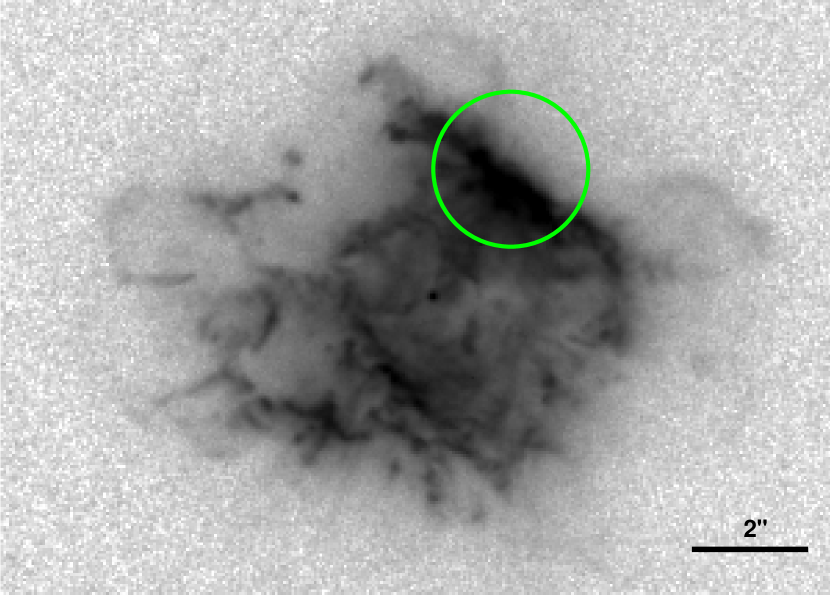
Figure 1: The HST/WFPC2 PC F658N image of J900. North is up and east is left. The green circle indicates the dimension and location of BOES’s fibre on this PN (central coordinate is RA(2000.0) = 06:25:57.2 and DEC(2000.0) = +17:47:29.5).

We secured the $3700-9300$ Å spectra using the fibre-fed BOES attached to the 1.8-m telescope at BOAO, S. Korea on 2012 February 13. BOES has a single 2K$\times$4K pixel E2V-4482 detector. We put a fibre entrance with 2.8^′′ aperture at a position as shown in Fig. 1. We employed a single 7200 sec to register the faint emission lines and a 300 sec exposure to avoid the saturation for the strongest lines such as [O iii] and H$\alpha$. The seeing was $\sim$2.1^′′, the sky condition was stable, but sometimes thin clouds were passing. For flux calibration, we observed HR 5501 at airmass = 1.23, while the airmass of J900 was $1.09-1.24$. For wavelength calibration and detector sensitivity correction, we took Th-Ar comparison and instrumental flat frames, respectively.

We reduced the data using NOAO/IRAF echelle reduction package in a standard manner, including over-scan subtraction, scattered light subtraction between echelle orders. We measured the average spectral resolution ($R$) of 42 770 using the full width at half maximum (FWHM) of 2825 Th-Ar comparison lines. We removed sky emission lines using ESO UVES sky emission spectrum after Gaussian convolution to matching BOES spectral resolution. The signal-to-noise ratio for continuum varies $\sim$$2-8$ with an average $\sim$4 over $3720-9220$ Å.

2.2 IUE UV, AKARI/IRC, and Spitzer/IRS mid-spectra

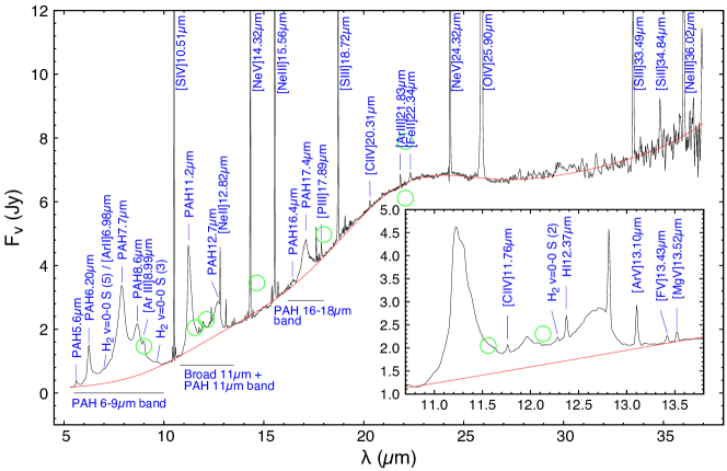
Figure 2: The Spitzer/IRS spectrum of J900. The flux density is scaled up to matching with AKARI, WISE, and MSX photometry (green circles). As a guide, we plot the continuum fit by 6-th order spline function (red line). The identified atomic lines, H₂, and PAH emission are indicated by the blue lines with labels. The $6-9$ µm, 11 µm, and $16-18$ µm PAH bands are also indicated by the horizontal lines. The inset displays the closeup of the $10.7-13.8$ µm spectrum in order to show the detected weak atomic gas emission such as [F v] 13.43 µm.

We chose the following dataset of the International Ultraviolet Explorer (IUE): SWP07965, 08677, and 53870 (these data cover $1150-1978$ Å, $R$$\sim$300) and LWR06938 and 07429 (these cover $1852-3348$ Å, $R$$\sim$400) from Mikulski Archive for Space Telescopes (MAST). For each SWP and LWR datum, we did average combining, so we connected these two resultant spectra into the single $1150-3348$ Å spectrum.

We utilised the AKARI/Infrared Camera (IRC; Onaka et al., 2007) $2.5-5.0$ µm spectrum ($R$$\sim$120) as presented in Ohsawa et al. (2016). We also analyse the Spitzer/IRS spectra taken with the Short-Low (SL, $5.2-14.5$ µm, $R$$\sim$60 – 130), Short-High (SH, $9.9-19.6$ µm, $R$$\sim$600), and Long-High modules (LH, $18.7-37.2$ µm, $R$$\sim$600). We downloaded the following Basic Calibrated Data (BCD): AORKEY 16921344, 20570368, 21458944, 24400640, 27018752, 27019008, 28538880, 28539136, 33777152, and 33777408. We reduced these BCD using the data reduction packages SMART v.8.2.9 (Higdon et al., 2004) and IRSCLEAN v.2.1.1. We normalised the flux density of the SL-, SH-, and LH-spectra in the overlapping wavelengths, and obtained a single $5.2-37.2$ µm spectrum. Then, we scaled the flux density of this spectrum to matching with AKARI, WISE, and MSX photometry (green circles) by a factor of 1.461 (see § 2.5 and 2.6 for details). The resultant spectrum with identifications of detected atomic and molecular gas emission lines is displayed in Fig. 2.

2.3 Interstellar extinction correction

Table 1: Calculated $c$(H$\beta$) values in J900 using H i Balmer (B$n_{\rm u}$, $n_{\rm u}$: the upper principal quantum number) and Paschen (P$n_{\rm u}$) series.

Line	$\lambda_{\rm lab}$ (Å)	$c$(H$\beta$)	Line	$\lambda_{\rm lab}$ (Å)	$c$(H$\beta$)
B10	3797.90	5.66(–1) $\pm$ 4.63(–2)	P14	8598.39	5.44(–1) $\pm$ 3.71(–3)
B9	3835.38	4.94(–1) $\pm$ 2.59(–2)	P13	8665.02	5.62(–1) $\pm$ 4.89(–3)
B3	6562.80	5.49(–1) $\pm$ 9.14(–3)	P12	8750.47	5.48(–1) $\pm$ 4.11(–3)
P15	8545.38	5.52(–1) $\pm$ 6.56(–3)	P11	8862.78	5.26(–1) $\pm$ 3.74(–3)

We measure emission line fluxes by multiple Gaussian component fitting. We correct the measured line fluxes $F$($\lambda$) to obtain the interstellar extinction corrected line fluxes $I$($\lambda$) using the formula;

$$I(\lambda)=F(\lambda)~{}\cdot~{}10^{c({\rm H\beta})(1+f(\lambda))},$$ (1)

where $f$($\lambda$) is the interstellar extinction function at $\lambda$ computed by the reddening law of Cardelli et al. (1989). Here, we adopt the average $R_{V}=3.1$ in the Milky Way. $c$(H$\beta$) is the reddening coefficient defined as $\log$$F$(H$\beta$)/$I$(H$\beta$).

For the BOES spectrum, we calculate $c$(H$\beta$) values (Table 1) by comparison of the observed Balmer and Paschen line ratios to H$\beta$ with their theoretical values of Storey & Hummer (1995) for the Case B assumption in an electron temperature $T_{\rm e}$ of 10⁴ K and an electron density $n_{\rm e}$ of 7000 cm^-3 (from the ratios of [Ar iv] $F$(4711 Å)/$F$(4740 Å) and [Cl iii] $F$(5517 Å)/$F$(5537 Å)), and we adopt the average $c$(H$\beta$) value of $0.54~{}\pm~{}0.02$. For the IUE spectrum, we adopt $c$(H$\beta$)$=0.57~{}\pm~{}0.06$ calculated by comparison of the He ii $F$(1640 Å)/$F$(2733 Å) with the theoretical ratio (30.81) by Storey & Hummer (1995) under the same assumption applied for the BOES spectrum. Due to negligibly small reddening, we do not correct the extinctions for the measured emission line fluxes and flux densities at the AKARI and Spitzer wavelengths.

2.4 Line flux normalisation

In Appendix Table A11, we list the identified lines. The successive columns are laboratory wavelengths, ions responsible for the line, extinction parameters $f(\lambda)$, line intensities $I$($\lambda$) on the scale of $I$(H$\beta$) = 100, and 1-$\sigma$ uncertainties of $I(\lambda)$. For the lines in the IUE spectra, we normalise the line fluxes with respect to the He ii 1640 Å, perform reddening correction, and multiply a constant factor of 235.1, which is determined from the theoretical Case B $I$(1640 Å)/$I$(4685 Å) ratio (6.558, Storey & Hummer, 1995) and the observed $I$(He ii 4685 Å)/$I$(H$\beta$) of 35.85/100 to express $I$(H$\beta$) = 100. For the lines in the Spitzer spectrum, we normalise the line fluxes with respect to the line at 12.37 µm, which is the complex of H i 12.37 µm ($n=6-7$, $n$ is the quantum number) and 12.39 µm ($n=8-11$). Then, we multiply all the normalised line fluxes by 1.043 in order to express $I$(H$\beta$) = 100 since the theoretical Case B $I$(12.37/12.39 µm)/$I$(H$\beta$) of 1.043/100 (Storey & Hummer, 1995). Similarly, we normalise the measured line fluxes in the AKARI spectrum with respect to the H i 4.05 µm, and then multiply 7.781 in order to express $I$(H$\beta$) = 100 as the theoretical Case B $I$(H i 4.05 µm)/$I$(H$\beta$) of 7.781/100 (Storey & Hummer, 1995).

2.5 Image and photometry data

We collected the data taken from the Hubble Space Telescope (HST)/Wide Field and Planetary Camera2 (WFPC2), Isaac Newton Telescope (INT) 2.5-m/Wide Field Camera (WFC), United Kingdom Infra-Red Telescope (UKIRT) 3.8-m/Wide Field Camera (WFCAM), Midcourse Space Experiment (MSX; Egan et al., 2003), Wide-field Infrared Survey Explorer (WISE; Cutri, 2014), AKARI/IRC (Ishihara et al., 2010), and Far Infrared Surveyor (FIS) (Yamamura et al., 2010). The detailed procedures are as follows.

We downloaded the raw Sloan $g$ and $r$ band images taken with the WFC mounted on the 2.5-m INT from the Cambridge Astronomical Survey Unit (CASU) Astronomical Data Centre. We reduced these data using NOAO/IRAF following a standard manner (i.e., bias subtraction, flat-fielding, bad-pixel masking, cosmic-ray removal, detector distortion correction, and sky subtraction), and performed PSF fitting for the surrounding star subtraction. And then, we performed aperture photometry for J900 and the standard star SA 113-260 and Feige 22 (Smith et al., 2002). Similarly, we downloaded the reduced $J$, $H$, and $K$ images taken with the WFCAM mounted on the 3.8-m UKIRT from the UKIRT WFCAM Science Archive (WSA). We measured$J$, $H$, and $K$ band magnitudes of J900 based on our own photometry of 77 nearby field stars, and converted these respective instrumental magnitudes into the $J$, $H$, and $K$ band magnitudes at the system of the Two Micron All Sky Survey (2MASS; Skrutskie et al., 2006).

In Appendix Table A2, we list the reddening corrected flux density $I_{\lambda}$ using eq (1) and $c$(H$\beta$)$=0.54~{}\pm~{}0.02$ (§ 2.3). We skip extinction correction in the photometry bands at the wavelengths longer than WISE W1 band. For HST/F555W, we perform photometry of the central star of the PN (CSPN) and the central star plus nebula. All the flux densities in the other bands are the sum of the radiation from the CSPN and nebula.

2.6 H$\beta$ flux of the entire nebula

Using a constant factor of $1.461~{}\pm~{}0.169$, we scale the Spitzer/IRS spectrum to match with WISE W3/W4 bands, MSX 12.13/14.65 µm bands, and AKARI/IRC S9W/L18W bands of Ishihara et al. (2010). H i 12.37+12.39 µm line flux is $(2.322~{}\pm~{}0.285)$(–13) erg s^-1 cm^-2, where $A(-B)$ means $A\times 10^{-B}$ hereafter. Thus, we obtain the extinction free H$\beta$ line flux of the entire nebula $(2.225~{}\pm~{}0.288)$(–11) erg s^-1 cm^-2 using the theoretical Case B $I$(H$\beta$)/$I$(12.37+12.39 µm) ratio.

3 Results

3.1 Plasma diagnostics

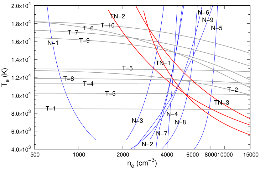
Figure 3: $n_{\rm e}-T_{\rm e}$ curves generated by the plasma diagnostic line ratios listed in Table 2. The blue, grey, and red lines are sensitive to $n_{\rm e}$, $T_{\rm e}$, and $T_{\rm e}$/$n_{\rm e}$, respectively. The ID of each curve is the same used in Table 2.

Table 2: Summary of plasma diagnostics of J900.

ID	CEL $n_{\rm e}$–diagnostic line	Value	Result (cm-3)
N-1	[N i] 5197 Å/5200 Å	$1.346~{}\pm~{}0.053$	$920~{}\pm~{}110$
N-2	[S ii] 6717 Å/6731 Å	$0.584~{}\pm~{}0.015$	$4360~{}\pm~{}490$
N-3	[O ii] 3726 Å/3729 Å	$1.773~{}\pm~{}0.067$	$3290~{}\pm~{}390$
N-4	[S iii] 18.7 µm/33.5 µm	$2.886~{}\pm~{}0.245$	$4660~{}\pm~{}590$
N-5	[Cl iii] 5517 Å/5537 Å	$0.683~{}\pm~{}0.020$	$8400~{}\pm~{}710$
N-6	[Cl iv] 11.8 µm/20.3 µm	$1.361~{}\pm~{}0.178$	$4470~{}\pm~{}1590$
N-7	[Ar iv] 4711 Å/4740 Å	$0.879~{}\pm~{}0.016$	$6090~{}\pm~{}340$
N-8	[Ne v] 14.3 µm/24.3 µm	$1.749~{}\pm~{}0.147$	$6500~{}\pm~{}1240$
ID	CEL $T_{\rm e}$–diagnostic line	Value	Result (K)
T-1	[O i] (6300/63 Å)/5577 Å	$96.719~{}\pm~{}7.203$	$8500~{}\pm~{}200$
T-2	[N ii] (6548/83 Å)/5755 Å	$57.138~{}\pm~{}1.147$	$12\,060~{}\pm~{}120$
T-3	[S iii] 9069 Å/6313 Å	$9.023~{}\pm~{}0.282$	$10\,190~{}\pm~{}140$
T-4	[Ar iii] (7751/7135 Å)/5191 Å	$125.043~{}\pm~{}9.734$	$11\,290~{}\pm~{}360$
T-5	[O iii] (4959/5007 Å)/4363 Å	$98.464~{}\pm~{}1.587$	$12\,850~{}\pm~{}80$
T-6	[Cl iv] (11.8 µm/20.3 µm)/7531 Å	$4.031~{}\pm~{}0.292$	$14\,920~{}\pm~{}880$
T-7	[Ar iv] (4711/40 Å)/(7170/7262 Å)	$25.503~{}\pm~{}0.893$	$15\,120~{}\pm~{}420$
T-8	[Ne iii] 15.8 µm/(3869/3967 Å)	$0.745~{}\pm~{}0.045$	$11\,640~{}\pm~{}230$
T-9	[Ar v] 13.10 µm/6435 Å	$8.138~{}\pm~{}0.641$	$14\,140~{}\pm~{}650$
T-10	[Ne iv] (2422/25 Å)/	$77.386~{}\pm~{}4.338$	$16\,330~{}\pm~{}510$
	(4714/15/24/26 Å)
ID	CEL $T_{\rm e}$/$n_{\rm e}$–diagnostic line	Value	Result (K)
TN-1	[S ii] (4069/76 Å)/(6717/31 Å)	$3.180~{}\pm~{}0.206$	$12\,180~{}\pm~{}1060$
TN-2	[O ii] (3726/29 Å)/(7320/30 Å)	$11.195~{}\pm~{}0.244$	$13\,000~{}\pm~{}240$
TN-3	[S iii] (18.7/33.5 µm)/9069 Å	$1.798~{}\pm~{}0.097$	$13\,920~{}\pm~{}960$
	RL $T_{\rm e}$–diagnostic line	Value	Result (K)
	He i 7281 Å/6678 Å	$0.204~{}\pm~{}0.006$	$9290~{}\pm~{}280$
	$[I_{\lambda}(8194\,\mbox{\AA})-I_{\lambda}(8169\,\mbox{\AA})]/I$(P11)	$0.022~{}\pm~{}0.003$	$9140~{}\pm~{}2540$

In Fig. 2, we plot $n_{\rm e}$–$T_{\rm e}$ curves using the collisionally excited line (CEL) ratios listed in Table 2. The adopted effective collision strengths $\Psi$($T$) and transition probabilities $A_{ji}$ ($i,j$: energy level, $E_{j}>E_{i}$) are listed in Appendix Table A3. For $T_{\rm e}$([O iii]) (ID: T-5) and $T_{\rm e}$([O ii]) (TN-2) curves, we subtract the recombination contributions of O³⁺ and O²⁺ to the [O iii] 4363 Å and the [O ii] 7320/30 Å using eqs. (2) and (3) of Liu et al. (2000), respectively; the corrected $I$([O iii] 4363 Å) and $I$([O ii] 7320/30 Å) are $14.281~{}\pm~{}0.219$ and $10.606~{}\pm~{}0.149$, respectively. Using the multiwavelength spectra allows us to trace $n_{\rm e}$ and $T_{\rm e}$ values in the regions throughout from the hot plasma close to the CSPN (e.g., [Ne v] with ionisation potential (IP) = 97.1 eV) to the cold and dusty photodissociation regions (PDRs).

We determine the $n_{\rm e}$ and $T_{\rm e}$ values at the intersection of $n_{\rm e}$(X) and $T_{\rm e}$(X) or $T_{\rm e}$(X)/$n_{\rm e}$(X) diagnostic curves for an ion X. The $T_{\rm e}$([O i]) and $n_{\rm e}$([N i]) values have been determined from their curves; two $T_{\rm e}$([S iii]) values are derived based on the $n_{\rm e}$([S iii] curve; and the $n_{\rm e}$([Cl iii]) is determined by the adoption of the average $T_{\rm e}$ value between two $T_{\rm e}$([S iii]) ones. For $T_{\rm e}$([Ar iii]), we utilised the other similar IP $n_{\rm e}$([Cl iii]) curve. The $T_{\rm e}$([O iii]) is determined from the $n_{\rm e}$([Cl iv]) curve; the $T_{\rm e}$([Ne iii]) is from the $n_{\rm e}$([Ar iv]) curve; and the $T_{\rm e}$([Ar v]) and $T_{\rm e}$([Ne iv]) are found from the $n_{\rm e}$([Ne v]).

Our derived CEL $T_{\rm e}$ and $n_{\rm e}$ are comparable to previous works, e.g., Kwitter et al. (2003) and Kingsburgh & Barlow (1992, 1994): $T_{\rm e}$([O iii]) = 11 600 K, $T_{\rm e}$([S iii]) = 13 000 K, $T_{\rm e}$([N ii]) = 11 500 K, $T_{\rm e}$([O ii]) = 10 300 K, $T_{\rm e}$([S ii]) = 7800 K, and $n_{\rm e}$([S ii]) = 3600 cm^-3 (10 $\%$ uncertainty) by Kwitter et al. (2003); $T_{\rm e}$([O iii]) = 12 000${}^{+400}_{-200}$ K, $n_{\rm e}$([O ii]) = 3980${}^{+790}_{-650}$ cm^-3, $n_{\rm e}$([Ar iv]) = 8240${}^{+7000}_{-3600}$ cm^-3 by Kingsburgh & Barlow (1992, 1994).

We compute $T_{\rm e}$(He i) using the He i $I$(7281 Å)/$I$(6678 Å) ratio by adopting the effective recombination coefficient $\alpha_{ji}$ listed in Appendix Table A4. We adopted $\alpha_{ji}$ of Benjamin et al. (1999) for $n_{\rm e}$ = 10⁴ cm^-3. $T_{\rm e}$(PJ) is calculated from the Paschen continuum discontinuity using eq. (7) of Fang & Liu (2011) and the ionic He⁺ and He²⁺ abundances (Appendix Table 6) under the derived $T_{\rm e}$(He i). Due to high uncertainty of $T_{\rm e}$(PJ), we calculate the recombination line (RL) C^2+,3+,4+ abundances by adopting $T_{\rm e}$(He i).

3.2 Ionic abundance derivations

Table 3: Comparison of our derived ionic abundances in J900 with Aller & Czyzak (1983, AC83), Kingsburgh & Barlow (1994, KB94), and Kwitter et al. (2003, K03). $T_{\rm e}$ adopted for calculations of each ionic abundance in our work, KB94, and K03 are listed in columns (3), (6), and (8), respectively.

Ion	Ours	Adopted $T_{\rm e}$ (K)	AC83	KB94	Adopted $T_{\rm e}$ (K)	K03	Adopted $T_{\rm e}$ (K)
(1)	$(2)$	in Ours (3)	(4)	(5)	in KB94 (6)	$(7)$	in K03 (8)
He+	$7.74(-2)~{}\pm~{}9.95(-3)$	$9290~{}\pm~{}280$	6.00(–2)	8.20(–2)	10 000?	$6.26(-2)~{}\pm~{}1.88(-2)$	$11\,500~{}\pm~{}1150$
He2+	$3.11(-2)~{}\pm~{}2.33(-3)$	$9290~{}\pm~{}280$	3.80(–2)	4.02(–2)	10 000?	$3.25(-2)~{}\pm~{}9.75(-3)$	$11\,500~{}\pm~{}1150$
C2+ (RL)	$1.05(-3)~{}\pm~{}1.23(-4)$	$9290~{}\pm~{}280$	9.63(–4)
C2+ (CEL)	$8.16(-4)~{}\pm~{}2.24(-4)$	$11\,800~{}\pm~{}490$	7.68(–4)	1.09(–3)	12 000
C3+ (CEL)	$1.10(-4)~{}\pm~{}3.43(-5)$	$14\,140~{}\pm~{}650$	2.61(–4)	3.64(–4)	13 000
N+	$6.80(-6)~{}\pm~{}1.37(-7)$	$12\,060~{}\pm~{}120$	4.76(–6)	9.44(–6)	9900	$5.40(-6)~{}\pm~{}1.62(-6)$	$11\,500~{}\pm~{}1150$
O0	$3.08(-5)~{}\pm~{}2.12(-6)$	$8500~{}\pm~{}200$				$7.21(-6)~{}\pm~{}2.16(-6)$	$11\,500~{}\pm~{}1150$
O+	$2.47(-5)~{}\pm~{}6.41(-7)$	$13\,000~{}\pm~{}240$	2.05(–5)	8.48(–5)	9900	$1.88(-5)~{}\pm~{}5.64(-6)$	$11\,500~{}\pm~{}1150$
O2+	$1.67(-4)~{}\pm~{}1.88(-6)$	$12\,850~{}\pm~{}80$	2.12(–4)	2.40(–4)	12 000	$2.14(-4)~{}\pm~{}6.42(-5)$	$11\,600~{}\pm~{}1160$
Ne2+	$7.17(-5)~{}\pm~{}2.79(-6)$	$11\,640~{}\pm~{}230$	4.85(–5)	5.53(–5)	12 000	$5.34(-5)~{}\pm~{}1.60(-5)$	$11\,600~{}\pm~{}1160$
Ne3+	$8.71(-6)~{}\pm~{}1.64(-6)$	$16\,330~{}\pm~{}510$	2.90(–5)
Ne4+	$3.50(-6)~{}\pm~{}2.00(-7)$	$16\,300~{}\pm~{}510$	3.80(–6)
S+	$2.48(-7)~{}\pm~{}1.28(-8)$	$12\,180~{}\pm~{}1060$	1.39(–8)	[1.87(–6)]	9900	$1.68(-7)~{}\pm~{}5.04(-8)$	$11\,500~{}\pm~{}1150$
S2+	$1.77(-6)~{}\pm~{}7.57(-8)$	$12\,060~{}\pm~{}550$	1.29(–6)			$1.54(-6)~{}\pm~{}4.62(-7)$	$13\,000~{}\pm~{}1300$
Cl2+	$3.38(-8)~{}\pm~{}2.19(-9)$	$11\,800~{}\pm~{}490$	2.40(–8)
Cl3+	$2.11(-8)~{}\pm~{}1.06(-9)$	$14\,920~{}\pm~{}880$	6.10(–8)			$2.45(-8)~{}\pm~{}7.35(-9)$	$11\,600~{}\pm~{}1160$
Ar2+	$6.02(-7)~{}\pm~{}2.79(-8)$	$11\,290~{}\pm~{}360$	3.05(–7)			$4.93(-7)~{}\pm~{}1.48(-7)$	$11\,600~{}\pm~{}1160$
Ar3+	$1.80(-7)~{}\pm~{}5.23(-9)$	$15\,120~{}\pm~{}420$	6.32(–7)	1.71(–7)	13 000	$2.57(-7)~{}\pm~{}7.65(-8)$	$11\,600~{}\pm~{}1160$
Ar4+	$4.72(-8)~{}\pm~{}2.90(-9)$	$14\,140~{}\pm~{}650$	1.08(–7)	3.11(–7)	14 270

3.2.1 The CEL ionic abundances

We solve atomic multiple energy-level population models for each ion by adopting $n_{\rm e}$–$T_{\rm e}$ pair (Appendix Table A5) to calculate the CEL ionic abundances. In Appendix Table 6, we summarise the resultant CEL ionic abundances with 1-$\sigma$ uncertainty. The first time measurement of 21 species out of our calculated 37 CEL ionic abundance is performed in this study. When more than one line for a targeting ion are detected, we compute ionic abundances using each line, and then we adopt the average value between the derived ionic abundances. The last line in boldface shows the adopted value.

Sixteen CEL ionic abundances calculated by previous works are summarised in Table 3. There are five measurements including ours since the pioneering work by Aller & Czyzak (1983), who used the image-tube scanner and IUE spectra and adopted $c$(H$\beta$) = 0.83 (no information on the adopted $n_{\rm e}$ and $T_{\rm e}$ though). The measurements of Kwitter et al. (2003) (their adopted $c$(H$\beta$) = 0.48) based on the $3600-9600$ Å spectrum reasonably agree with ours, except for O⁰, S²⁺, and Ar³⁺. The difference in these ionic abundances is mainly due to the adopted $T_{\rm e}$ as listed in the column (6) of Table 3. O⁰, S²⁺, and Ar³⁺ are ($1.25~{}\pm~{}0.14$)(–5), ($2.39~{}\pm~{}0.22$)(–6), and ($2.91~{}\pm~{}0.12$)(–7), which are close to the relevant values of Kwitter et al. (2003). The difference between Kingsburgh & Barlow (1994) and ours is attributable to the adopted $c$(H$\beta$) (0.80). In particular, the difference $c$(H$\beta$) affects the intensity corrections of the lines in the UV wavelength. Kingsburgh & Barlow (1994) reported that S⁺ abundance was determined using [S ii] 6717/31 Å lines, but we were not able to find the information from their Table 3, so we could not find which caused the difference in their derived S⁺ and elemental S abundances. The previous works calculated the CEL ionic abundances using very limited numbers of the $n_{\rm e}$–$T_{\rm e}$ pairs, whereas we select $n_{\rm e}$–$T_{\rm e}$ optimised for each ionic abundance. Thus, we conclude that our derived CEL ionic abundances are more reliable than ever.

3.2.2 Detection of F, Rb, Kr, and Xe lines and their abundances

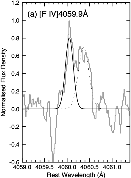
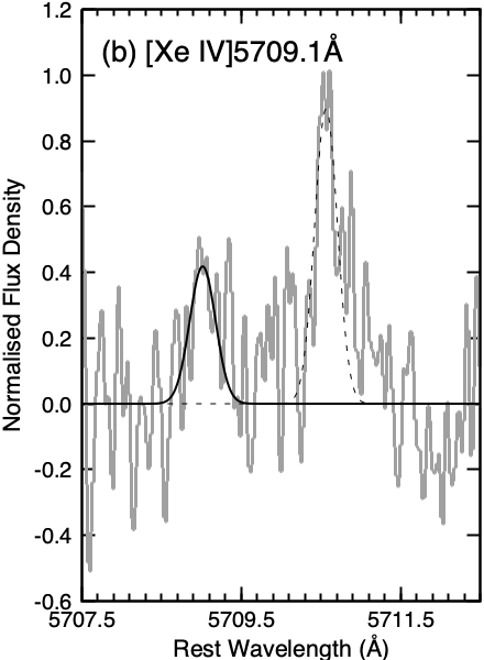
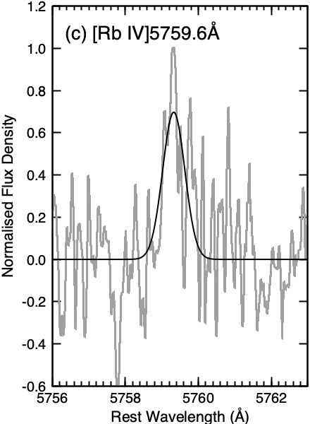
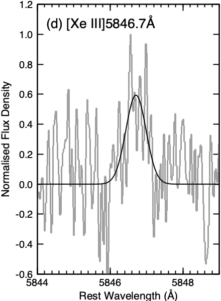
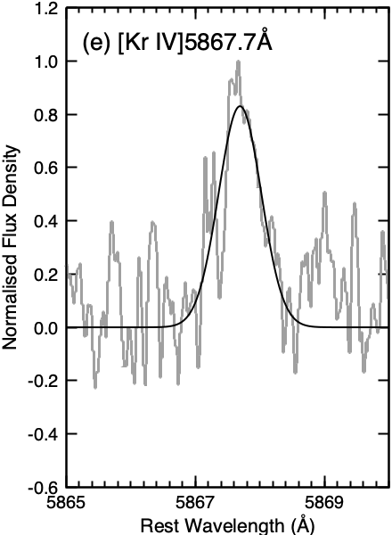
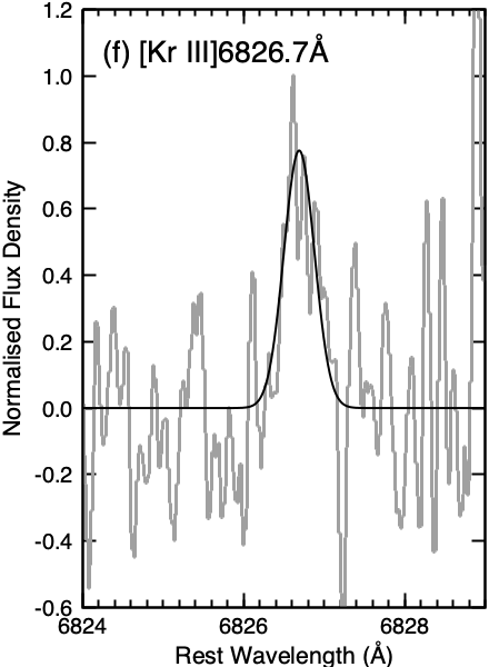
Figure 4: The identified emission lines of F, Kr, Rb, and Xe. The grey and black lines are the observed spectrum and the Gaussian fitting result, respectively. The dotted line profile in panels (a) and (b) is the fitting result of N ii 4060.20 Å and 5710.77 Å lines, respectively. The contribution from He ii lines to [Rb iv] 5759.6 Å and [Xe iii] 5846.7 Å is subtracted. Contamination of skylines to [Kr iii] 6826.7 Å is subtracted out.

F abundances have been calculated in only 16 PNe, so far (Zhang & Liu, 2005; Otsuka et al., 2008, 2011; Otsuka et al., 2015). The FWHM of the detected line centred at $\lambda_{\rm c}=13.42$ µm is 0.025 µm, so we consider $[$Mn vi$]$ 13.40 µm, He i 13.42-13.44 µm, and [F v] 13.43 µm lines as candidates. The possibility of $[$Mn vi$]$ 13.40 µm and He i has been ruled out as our Cloudy model does not predict these Mn and He i lines with detectable intensity in the Spitzer/IRS spectrum. Our Cloudy model can reproduce the observed [F iv] and [F v] line intensities with a consistent F abundance, simultaneously (we demonstrate in § 4). Thus, the identification of [F v] 13.43 µm and [F iv] 4059.9 Å lines (Fig. 4(a)) is likely to be appropriate and then the [F v] 13.43 µm line would be firstly identified in J900.

Rb has been discovered in only a handful of PNe (Sterling et al., 2016; Mashburn et al., 2016; Madonna et al., 2017; Madonna et al., 2018) since the first measurement of García-Rojas et al. (2015). We also detect [Xe iv] 5709.1 Å (Fig. 4(b)) and [Rb iv] 5759.56 Å lines (Fig. 4(c)) in J900 for the first time. Besides, we confirm the presence of [Xe iii] 5846.7 Å (Fig. 4(d)), [Kr iv] 5867.7 Å (Fig. 4(e)), and [Kr iii] 6826.7 Å (Fig. 4(f)) firstly done by Sterling et al. (2009).

In order to accurately calculate Rb³⁺, we subtract the He ii line contribution to the [Rb iv] 5759.55 Å using the theoretical ratio of the He ii $I(5759.64\,\mbox{\AA})/I(5852.67\,\mbox{\AA})$ (0.39; Storey & Hummer, 1995). Fig. 4(c) shows the residual spectrum after subtracting He ii 5759.64 Å out. For J900, Sterling et al. (2009) reported the detection of above Xe and Kr lines, but the Xe^2+,3+ and Kr³⁺ had never been calculated. Similarly, we subtract the contribution of He ii 5846.66 Å using the theoretical ratio of He ii $I(5846.66\,\mbox{\AA})/I(5857.26\,\mbox{\AA})$ (0.914; Storey & Hummer, 1995). The residual spectrum after this process is shown in Fig. 4(d).

Sterling & Dinerstein (2008) calculated Kr²⁺ to be ($1.28~{}\pm~{}0.61$)(–9) under $T_{\rm e}$([O iii]) = $11\,600~{}\pm~{}1160$ K and $n_{\rm e}$ = $3600~{}\pm~{}720$ cm^-3 using the $T_{\rm e}$-insensitive fine-structure line [Kr iii] 2.199 µm. Perhaps, more careful treatment for their Kr²⁺ value is necessary as Sterling & Dinerstein (2008) pointed out that the line at 2.199 µm would be the complex of the [Kr iii] 2.199 µm and H₂ $v=3-2$ S(3) at 2.201 µm lines. Despite this, our derived Kr²⁺ using the $T_{\rm e}$-sensitive [Kr iii] 6826.70 Å line (Fig. 4(f)) is consistent with the value of Sterling & Dinerstein (2008). This unexpected outcome implies that the H₂ $v=3-2$ S(3) contribution to the [Kr iii]  2.199 µm is negligible, suggesting that intensity measurement of both of Kr lines and our adopted $T_{\rm e}$ for Kr²⁺ using [Kr iii] 6826.70 Å is reasonable.

3.2.3 The RL ionic abundances

The RL He^+,2+ and C^2+,3+,4+ are summarised in Appendix Table 6. We adopt $T_{\rm e}$(He i) and $n_{\rm e}$ = 10⁴ cm^-3. Aller & Czyzak (1983) did not give information on which He i,ii lines they used. In the earlier studies, Kingsburgh & Barlow (1994) used 3 He i/1 He ii lines and Kwitter et al. (2003) seems to use the He i 5875 Å and He ii 4686 Å lines only. Meanwhile, we use the 9 He i and 12 He ii lines to determine the final He⁺ and He²⁺, in order to minimise the uncertainty of their ionic abundances.

In Appendix Table 6, our final RL C^2+,3+,4+ and associated standard deviation errors are given. The RL C²⁺ using C ii 4267 Å only had been measured in Aller & Czyzak (1983) and Kingsburgh & Barlow (1994), whereas our work newly provides RL C^3+,4+. Our derived RL He^+,2+ and C²⁺ agree with the previous measurements (Table 3).

The degree of the discrepancy between RL and CEL ionic/elemental abundances, i.e., abundance discrepancy factor (ADF) defined as the ratio of the RL to CEL abundances, is derived. The ADF(C²⁺) of $1.29~{}\pm~{}0.38$ is consistent with both the value calculated from Aller & Czyzak (1983, 1.25, see Table 3) and the average ADF(C²⁺) amongst 6 C-rich PNe displaying the CEL C/O ratio $>1$ in Delgado-Inglada & Rodríguez (2014, $1.41~{}\pm~{}0.58$).

3.3 Elemental abundances

Table 4: Elemental abundances of J900. $\epsilon({\rm X})=12+\log\,({\rm X/H})$, where $\log$ H is 12. AC83, KB94, K03, and SD08 mean Aller & Czyzak (1983), Kingsburgh & Barlow (1994), Kwitter et al. (2003), and Sterling & Dinerstein (2008), respectively. S derived by Kingsburgh & Barlow (1994) seems to be overestimated (§ 3.2). The last columns are the derived abundances with respect to the solar abundances, defined as [X/H] = $\epsilon({\rm X})({\rm Ours})-\epsilon({\rm X})_{\sun}$, except for Se. [Se/H] = $\epsilon({\rm Se})({\rm AD08})-\epsilon({\rm X})_{\sun}$. We take $\epsilon$(X)_☉ of Lodders (2010) in the column (8) and those of Asplund et al. (2009) in the column (9).

X	X/H(Ours)	$\epsilon({\rm X})$(Ours)	$\epsilon({\rm X})$(AC83)	$\epsilon({\rm X})$(KB94)	$\epsilon({\rm X})$(K03)	$\epsilon({\rm X})$(SD08)	[X/H]Lo(Ours)	[X/H]As(Ours)
(1)	(2)	(3)	(4)	(5)	(6)	(7)	(8)	(9)
He	$1.08(-1)~{}\pm~{}1.02(-2)$	$11.04~{}\pm~{}0.04$	$10.99$	$11.09$	$11.00~{}\pm~{}0.13$		$+0.11~{}\pm~{}0.05$	$+0.11~{}\pm~{}0.04$
C(CEL)	$1.09(-3)~{}\pm~{}2.60(-4)$	$9.04~{}\pm~{}0.10$	$9.10$	$9.31$			$+0.65~{}\pm~{}0.11$	$+0.57~{}\pm~{}0.12$
C(RL)	$2.01(-3)~{}\pm~{}7.08(-4)$	$9.30~{}\pm~{}0.15$					$+0.91~{}\pm~{}0.16$	$+0.87~{}\pm~{}0.16$
N	$6.93(-5)~{}\pm~{}1.82(-5)$	$7.84~{}\pm~{}0.11$	$7.77$	$7.64$	$8.01~{}\pm~{}0.09$		$-0.02~{}\pm~{}0.17$	$-0.03~{}\pm~{}0.12$
O	$2.95(-4)~{}\pm~{}1.11(-5)$	$8.47~{}\pm~{}0.02$	$8.50$	$8.59$	$8.55~{}\pm~{}0.06$		$-0.26~{}\pm~{}0.07$	$-0.26~{}\pm~{}0.05$
F	$1.45(-7)~{}\pm~{}2.45(-8)$	$5.16~{}\pm~{}0.07$					$+0.72~{}\pm~{}0.09$	$+0.70~{}\pm~{}0.31$
Ne	$8.89(-5)~{}\pm~{}3.26(-6)$	$7.95~{}\pm~{}0.02$	$7.91$	$8.00$	$7.95~{}\pm~{}0.09$		$-0.10~{}\pm~{}0.10$	$-0.02~{}\pm~{}0.10$
Mg	$2.22(-5)~{}\pm~{}3.17(-6)$	$7.35~{}\pm~{}0.06$					$-0.19~{}\pm~{}0.09$	$-0.29~{}\pm~{}0.07$
Si	$9.33(-6)~{}\pm~{}3.07(-6)$	$6.97~{}\pm~{}0.14$					$-0.56~{}\pm~{}0.16$	$-0.58~{}\pm~{}0.15$
P	$3.06(-7)~{}\pm~{}3.45(-8)$	$5.49~{}\pm~{}0.05$					$+0.04~{}\pm~{}0.07$	$+0.02~{}\pm~{}0.06$
S	$3.43(-6)~{}\pm~{}1.26(-7)$	$6.53~{}\pm~{}0.02$	$6.38$	$[7.22]$	$6.33~{}\pm~{}0.16$		$-0.63~{}\pm~{}0.03$	$-0.63~{}\pm~{}0.03$
Cl	$7.47(-8)~{}\pm~{}1.45(-9)$	$4.80~{}\pm~{}0.03$	$5.09$		$4.59~{}\pm~{}0.10$		$-0.45~{}\pm~{}0.07$	$-0.43~{}\pm~{}0.30$
Ar	$8.94(-7)~{}\pm~{}3.29(-8)$	$5.95~{}\pm~{}0.02$	$6.07$	$5.49$	$6.08~{}\pm~{}0.09$		$-0.55~{}\pm~{}0.10$	$-0.49~{}\pm~{}0.13$
K	$2.73(-8)~{}\pm~{}4.51(-9)$	$4.44~{}\pm~{}0.07$					$-0.67~{}\pm~{}0.08$	$-0.64~{}\pm~{}0.12$
Fe	$6.69(-7)~{}\pm~{}3.20(-8)$	$5.83~{}\pm~{}0.21$					$-1.63~{}\pm~{}0.22$	$-1.71~{}\pm~{}0.21$
Se						$3.65~{}\pm~{}0.25$	$+0.32~{}\pm~{}0.25$	$+0.34~{}\pm~{}0.25$
Kr	$7.11(-9)~{}\pm~{}7.40(-10)$	$3.85~{}\pm~{}0.05$				$3.80~{}\pm~{}0.30$	$+0.57~{}\pm~{}0.09$	$+0.60~{}\pm~{}0.08$
Rb	$7.28(-10)~{}\pm~{}2.16(-10)$	$2.86~{}\pm~{}0.13$					$+0.48~{}\pm~{}0.13$	$+0.32~{}\pm~{}0.16$
Xe	$2.61(-9)~{}\pm~{}4.59(-10)$	$3.42~{}\pm~{}0.08$					$+1.15~{}\pm~{}0.11$	$+1.18~{}\pm~{}0.10$

We derive the elemental abundances by applying ionisation correction factor ICF(X) for element X. ICFs recover the ionic abundances in the unseen ionisation stages in the wavelength coverage by the IUE, BOES, AKARI/IRC, and Spitzer/IRS spectra. The abundance of the element X, which is the number density ratio with respect to hydrogen, is expressed by the following equation.

$${\rm X/H}={\rm ICF(X)}~{}\times\Sigma_{\rm m}~{}({\rm X}^{\rm m+}/{\rm H}^{+}).$$ (2)

Except for He, C(CEL), O, Ne, S, and Ar (whose ICFs are 1), we determine ICF(X) based on the IP of the element X. To determine each ICF definition and ICF values for each element, we refer to the mean ionisation fraction predicted in the Cloudy model of the highly-excited C-rich PN NGC6781 by Otsuka et al. (2017), simply because NGC6781 is very similar to J900 in many respects, including the effective temperature of the central star ($\sim$120 000 K), nebula shape (bipolar nebula), and dust and molecular gas features (C-dust dust and PAH/H₂), suggesting that the ionisation fraction would also be similar between the two objects. Note that we do not apply the empirical ICF values determined in NGC6781 to J900.

We define that C is the sum of C^+,2+,3+,4+. For the CEL C, we correct C⁴⁺ using ICF(C) = $1.26~{}\pm~{}0.24$ calculated from eq. (A25) of Kingsburgh & Barlow (1994). For the RL C, we correct C⁺ using ICF(C) = ($1-{\rm(C^{+}/C)_{CEL}}$)^-1. ICF(N) of $1.54~{}\pm~{}0.06$ corresponds to the O/(O⁺ + O²⁺), where the O is the sum of O^+,2+,3+. The theoretical model by Otsuka et al. (2017) predicted that the F, Ne, and Mg ionic fractions are very similar, so we determine ICF(F,Mg) = $7.28~{}\pm~{}1.02$ from the Ne/(Ne³⁺ + Ne⁴⁺) ratio. Assuming that Cl is the sum of Cl^+,2+,3+,4+, we determine ICF(Cl) = $1.06~{}\pm~{}0.06$ from Ar/(Ar⁺ + Ar²⁺ + Ar³⁺). As the fractional ionic stages of Si, P, and K are similar to that of S in the model of Otsuka et al. (2017), we adopt ICF(Si) of $10.16~{}\pm~{}2.88$ from the S/S⁺ ratio; ICF(P) is $1.70~{}\pm~{}0.09$ from the S/(S⁺ + S²⁺) ratio; and ICF(K) = $4.96~{}\pm~{}0.23$ from the Ar/Ar³⁺ ratio, respectively. ICF(Fe) of $11.96~{}\pm~{}0.55$ corresponds to the O/O⁺. Since the cross-section and recombination coefficients for Kr, Xe, and Rb are not fully determined yet, we cannot use the ICF(Kr,Xe,Rb) values predicted by photoionisation models. Thus, the use of the ICF(Kr,Rb,Xe) based on the ionisation potential is currently best. ICF(Kr) is $1.70~{}\pm~{}0.05$ calculated using eq. (4) of Sterling et al. (2015). ICF(Xe) is as same as ICF(Kr). ICF(Rb) is $1.76~{}\pm~{}0.07$ from the O/O²⁺ ratio by following Sterling et al. (2016).

In Appendix Table 4, we summarise the derived elemental abundances (X/H, second column), $\epsilon$(X) corresponding to 12 + $\log$ (X/H) (third column), and the abundances relative to the Sun [X/H] (last two columns).

Delgado-Inglada et al. (2015) concluded that Cl and Ar abundances are the best metallicity indicators based on chemical abundance analysis of 20 Galactic PNe. They argued that their abundances indicate the composition in the primordial gas clouds where the PN progenitors were born. Following their reasoning and the derived average [Cl,Ar/H] abundance (–0.50), we conclude that J900 was born in an environment with the metallicity $Z\sim 0.005$.

Potassium (K) is a volatile element ($\sim$50 % condensation temperature is $\sim$1000 K) considered to be synthesised mainly via the O-burning in massive stars. The evolution of K in the Galaxy seems to be similar to that of $\alpha$-elements, according to Takeda et al. (2009). The observed [K/H] abundance is comparable to the observed abundances of heavy $\alpha$-elements and Cl. Our derived extremely small [Fe/H] does not represent the metallicity of J900, judging from the derived [Cl,Ar/H]. We will discuss elemental abundances by comparison with the AGB nucleosynthesis models later.

3.4 Physical conditions of the H₂ lines

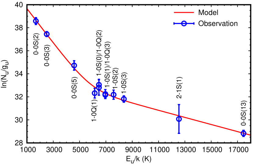
Figure 5: Excitation diagram of H₂ in J900. The H₂ lines in near-IR are taken from Hora et al. (1999). The H₂ intensities used in this plot are listed in Table 5. The red line is the best fit curve to the observed data with two temperatures = $667~{}\pm~{}54$ K and $3247~{}\pm~{}268$ K. See text for details.

Table 5: The H₂ line intensity in J900. H99 means Hora et al. (1999).

Line	$\lambda$ (µm)	$I($H2) (erg s-1 cm-2 sr-1)	Source
H2 $v=0-0$ S(2)	$12.293$	$1.81(-5)~{}\pm~{}5.41(-6)$	This work
H2 $v=0-0$ S(3)	$9.664$	$9.72(-5)~{}\pm~{}2.10(-5)$	This work
H2 $v=0-0$ S(5)	$6.910$	$7.29(-5)~{}\pm~{}2.98(-5)$	This work
H2 $v=0-0$ S(13)	$3.846$	$1.70(-5)~{}\pm~{}6.72(-6)$	This work
H2 $v=1-0$ Q(3)	$2.423$	$3.83(-5)~{}\pm~{}1.49(-5)$	H99
H2 $v=1-0$ Q(2)	$2.413$	$2.23(-5)~{}\pm~{}1.06(-5)$	H99
H2 $v=1-0$ Q(1)	$2.407$	$2.77(-5)~{}\pm~{}1.17(-5)$	H99
H2 $v=2-1$ S(1)	$2.248$	$8.51(-6)~{}\pm~{}1.06(-5)$	H99
H2 $v=1-0$ S(0)	$2.223$	$1.60(-5)~{}\pm~{}1.06(-5)$	H99
H2 $v=1-0$ S(1)	$2.122$	$5.11(-5)~{}\pm~{}1.17(-5)$	H99
H2 $v=1-0$ S(2)	$2.033$	$2.66(-5)~{}\pm~{}1.06(-5)$	H99
H2 $v=1-0$ S(3)	$1.957$	$7.34(-5)~{}\pm~{}2.02(-5)$	H99

It is necessary to determine the physical conditions of the regions giving rise to the H₂ lines in order to infer hydrogen density ($n_{\rm H}$) in the cold PDRs beyond the ionisation front. These PDRs are critically important in assessing how the progenitor ejected its dust and gas mass. Hence, we investigate H₂ temperature $T$(H₂) and column density $N$(H₂) under the local thermodynamic equilibrium (LTE) using excitation diagram (Fig. 5) based on the mid-IR H₂ lines $v=0-0$ S(2) 12.29 µm, S(3) 9.66 µm, and S(5) 6.91 µm in the Spitzer/IRS spectrum (Fig. 2), and S(13) 3.85 µm in the AKARI/IRC spectrum, and the near-IR H₂ lines by Hora et al. (1999).

The H₂ column density in the upper state $N_{u}$ is written as

$$N_{u}=\frac{4\pi I({\rm H_{2}})}{A}\cdot\frac{\lambda}{hc},$$ (3)

where $I$(H₂) is the H₂ line intensity in erg s^-1 cm^-2 sr^-1 (Table 5), $A$ is the transition probability taken from Turner et al. (1977), $h$ is the Planck constant, and $c$ is the speed of light. In LTE, the Boltzmann equation relates $N_{u}$ to the $T$(H₂) and $N$(H₂) via

$${\rm ln}\,\bigl{(}\frac{N_{u}}{g_{u}}\bigr{)}=-\frac{E_{u}}{kT({\rm H}_{2})}+{\rm ln}\,\bigl{[}N({\rm H}_{2})\cdot\frac{hcB}{2kT({\rm H}_{2})}\bigr{]},$$ (4)

where $g_{u}$ is the vibrational degeneracy, $E_{u}$ is the energy of the excited level taken from Dabrowski (1984), $k$ is the Boltzmann constant, and $B$ is the rotational constant (60.81 cm^-1).

Fig. 5 shows the plot of $\ln\,(N_{u}/g_{u})$ versus $E_{u}/k$, based on eq. (4). Note that the plot consists of two regimes relative to the x-axis $E_{u}/k\sim 6000$ K, perhaps representing the two different temperature components: the derived $T({\rm H}_{2})$ and $N$(H₂) for the warm temperature component ($E_{u}/k\lesssim 6000$ K) are $667~{}\pm~{}54$ K and $(1.14~{}\pm~{}0.29)$(+19) cm^-2, and those for the hot component ($E_{u}/k\gtrsim 6000$ K) are $3247~{}\pm~{}268$ K and $(5.38~{}\pm~{}1.37)$(+16) cm^-2, respectively. When we fit the H₂ lines at 6.91, 9.68, and 12.28 µm only, we obtain $T$(H₂) = $755~{}\pm~{}36$ K and $N$(H₂) = $(8.85~{}\pm~{}0.39)$(+18) cm^-2, respectively. We interpret that the H₂ lines with $E_{u}/k\gtrsim 6000$ K emit in the regions just outside the ionised nebula. There, the fast central star wind interacts with the slowly expanding AGB mass-loss. Meanwhile, H₂ lines with $E_{u}/k\lesssim 6000$ K would emit in the outermost of such wind interaction regions. Accordingly, the wind-wind interaction is anticipated to create the regions with a temperature gradient varying from $\sim$3300 to $\sim$700 K.

Excluding the mid-IR H₂ data and applying single temperature fitting towards the near H₂ data, we obtain $T$(H₂) of $2736~{}\pm~{}703$ K for the hot component, which is in agreement with Hora et al. (1999) who estimated $T$(H₂) of $2200~{}\pm~{}100$ K with a single temperature component fitting. Isaacman (1984a) and Hora et al. (1999) concluded that H₂ is emitted by thermal shocks rather than UV fluorescence. Our excitation diagram supports their conclusion.

3.5 PAH and Dust features

Aitken & Roche (1982) fit $8-13$ µm spectra using the emissivities of graphite grains and PAHs. Graphite grains have a broad feature around 30 µm. However, the Spitzer/IRS spectrum does not display such a broad feature. Thus, the carrier of the dust continuum (indicated by the red line in Fig. 2) would be amorphous carbon.

J900 exhibits several prominent broad emission features in $6-9$ µm, 11 µm, and $15-20$ µm overlying the dust continuum. They would be attributed to PAHs composing of a large number of C-atoms ($>$50; Peeters et al., 2017). The emission bands at 6.2, 7.7 µm, and 8.6 µm are charged PAHs, while that at 11.3 µm is neutral PAH (Peeters et al., 2017).

Following the classification of Matsuura et al. (2014), respective PAH $6-9$ µm and 11 µm band profiles would be divided into classes $\mathcal{B}$ and $\alpha$, where Galactic and Large Magellanic PNe have been grouped (e.g., Otsuka, 2015; Bernard-Salas et al., 2009). J900 displays the 16.4 and 17.4 µm emission features in the PAH $15-20$ µm band (Boersma et al., 2010, and reference therein). Through a detailed analysis of the PAH $15-20$ µm band, Boersma et al. (2010) reached conclusions that (1) 16.4/17.4/17.8/18.9 µm emission features do not correlate with each other and their carriers are independent molecular species and (2) the PAH 16.4 µm features only has a tentative connection with PAH 6.2/7.7 µm. Indeed, we confirm that the $I$(6.2 µm)/$I$(11.2 µm) and $I$(16.4 µm)/$I$(11.2 µm) ratios ($0.812~{}\pm~{}0.148$ and $0.013~{}\pm~{}0.002$, respectively, Appendix Table A11) are along a correlation found in Fig. 5 of Boersma et al. (2010). Later, Peeters et al. (2012) reported that the PAHs 12.7 and 16.4 µm emission correlate with the PAHs 6.2 and 7.7 µm, which arise from species in the same conditions that favour PAH cations. Following Boersma et al. (2010) and Peeters et al. (2012), we conclude that the 6.2/7.7/8.6/12.7/16.4 µm emission arise from charged PAHs and the 11.3 µm emission arises from neutral PAHs.

The carrier of the 17.4 µm band is under debate; certainly, mid-IR fullerene C₆₀ bands show four emission features at 7.0/8.5/17.4/18.9 µm (e.g., Cami et al., 2010; Otsuka et al., 2014), but three emission features at 7.0/8.5/18.9 µm are not seen in J900. Peeters et al. (2017) suggested charged PAHs, while Fig. 22 of Sloan et al. (2014) indicates an aliphatic compound alkyne chain, 2,4-hexadiyne, displaying a strong emission feature.

The ratio of neutral PAH $I$(3.3 µm)/$I$(11.3 µm) is directly related to the internal energy of the molecule. Therefore, given the internal energy, the ratio provides the number of C-atoms ($N_{\rm C}$) composing PAH molecules (Allamandola et al., 1987). Using the function of $I$(3.3 µm)/$I$(11.3 µm) versus $N_{\rm C}$ established in Ricca et al. (2012) and the observed AKARI/IRC PAH 3.3 µm to Spitzer/IRS 11.3 µm flux ratio ($0.15~{}\pm~{}0.01$, Appendix Table A11), we estimate $N_{\rm C}$ to be $\sim$150. This ratio is consistent with the value measured in a high-excitation PN NGC7027 (0.13; Otsuka et al., 2014).

4 Photoionisation modelling

To understand the evolution of J900, we investigate the current evolutionary status of the CSPN and the physical conditions of the gas and the dust grains by constructing a coherent Cloudy photoionisation model to be consistent with all the observed quantities of the CSPN and the dusty nebula. Below, we explain how to constrain the input parameters and obtain the best fit.

4.1 Modelling approach

Incident SED

For the incident SED of the CSPN, we adopt a non-LTE stellar atmosphere model grid of Rauch (2003). As an initial guess value, we adopt an effective temperature ($T_{\rm eff}$) of 134 800 K calculated using the observed $I$(He ii 4686 Å)/$I$(H$\beta$) ratio and the eq (3.1) established in Dopita & Meatheringham (1991). We adopt the surface gravity $\log\,g$ of 6.0 cm s^-2 by referring to the post-AGB evolution models of Miller Bertolami (2016). We scale the flux density of the CSPN’s SED to match with the observed HST/F555W magnitude of the CSPN (Table A2).

Distance $D$

For comparison between the model predicted values and the observations, we have to fix the distance $D$ towards J900. $D$ ranges from 3.89 to 5.82 kpc in literature (Kingsburgh & Barlow, 1992; Stanghellini et al., 2008; Stanghellini & Haywood, 2010; Giammanco et al., 2011; Frew et al., 2016; Stanghellini & Haywood, 2018) of which the average $D$ is 4.65 kpc (1-$\sigma$ = 0.72 kpc). The test model with $D=4.6$ kpc predicts that the ionisation front locates at $\sim$8.5^′′ away from the CSPN whereas the HST/F656N image suggests $\sim$3.5^′′. After several test model runs with different $D$ values, we find that the models with $D$ of $\sim$6.0 kpc can reproduce the ionisation front radius of $\sim$3.5^′′. Hence, we keep $\log\,g=6.0$ cm s^-1 and F555W magnitude of the CSPN and $D$ of 6.0 kpc during the iterative model fitting, whereas we vary $T_{\rm eff}$ to search for the best-fit model parameters that would reproduce the observational data.

Nebula geometry and hydrogen density profile

We adopt the cylindrical geometry with a height of 3^′′. The input radial hydrogen number density profile, $n_{\rm H}(R)$ ($R$ is the distance from the CSPN) in $R\leq 3.5^{\prime\prime}$ is to be determined based on our plasma diagnostics. As the average $n_{\rm e}$ is 4960 cm^-3 amongst $n_{\rm e}$([O ii]), $n_{\rm e}$([S iii]), $n_{\rm e}$([Cl iii]), $n_{\rm e}$([Cl iv]), $n_{\rm e}$([Ar iv]), and $n_{\rm e}$([Ne v]), we adopt a constant 4000 cm^-3 by taking the reasonable assumption that $n$(H⁺) is $n_{\rm e}$/1.15.

Assuming pressure equilibrium at the ionisation front, $n_{\rm H}$($R>3.5^{\prime\prime}$) is approximately 2$n_{\rm e}$$T_{\rm e}$/$T$(H₂). The factor of 2 is because the gas within the ionisation front is totally ionised and so has both electrons and protons. The [S ii] lines often indicate the physical conditions of the transition zone between ionised and neutral gases. Adopting $n_{\rm e}$([S ii]) and $T_{\rm e}$([S ii]), $n_{\rm H}$($R>3.5^{\prime\prime}$) is $\sim$($3.3-15.6$)$\times$10⁴ cm^-3. We further searched for values of $n_{\rm H}$($R>3.5^{\prime\prime}$) that can reproduce the observed mid-IR H₂ line fluxes based on the results of a small grid model with a constant $n_{\rm H}$($\leq 3.5^{\prime\prime}$) = 4000 cm^-3 and different values of $n_{\rm H}$($R>3.5^{\prime\prime}$). As discussed by Otsuka et al. (2017), it would be difficult to reproduce the observed H₂ line fluxes by the CSPN heating only. Thus, we add a constant temperature region in the PDRs using the “temperature floor” option, and we finally found a model, with $n_{\rm H}(R>3.5^{\prime\prime})=87\,500$ cm^-3, that reasonably matches the observed mid-IR H₂ line fluxes.

By following the method of Mallik & Peimbert (1988), we calculate the filling factor ($f$), which is the ratio of the root mean square $n_{\rm e}$ to the forbidden line $n_{\rm e}$. We keep the derived $f=0.75$ throughout model iteration.

$\epsilon$(X) / Dust grains and PAH molecules

Elements up to Zn can be handled in Cloudy. In the model calculations, we updated the originally installed $A_{ji}$ and $\Omega$($T_{\rm e}$) of forbidden C/N/O/F/Ne/Mg/P/S/Cl/Ar/K lines with the values in Appendix Table A3. For the first guess, we adopt the empirically determined $\epsilon$(X) listed in Table 4, except for Se, Kr, Rb, and Xe whose atomic data are not installed in Cloudy. We adopt the CEL $\epsilon$(C) as the representative carbon abundance. For the unobserved elements, we adopt the predicted $\epsilon$(X) by the AGB nucleosynthesis model of Karakas et al. (2018) for a star of initial metallicity $Z=0.003$ and 2.0 M_☉.

As J900 is a PN rich in carbon dust (§ 3.5), we run test models to determine which carbon grain’s thermal emission can fit the observed mid-IR SED. In these tests, we consider the optical data of graphite and amorphous carbon provided by Rouleau & Martin (1991). As we explained in § 3.5, the graphite grain models do not fit the observed SED at all due to the emission peak around 30 µm. Rouleau & Martin (1991) provided two types of optical constants measured from samples “BE” (soot produced from benzene burned in air) and “AC” (soot produced by striking an arc between two amorphous carbon electrodes in a controlled Ar atmosphere). A comparison between the AC and the BE model SEDs shows that the former gives the better fit to the observed SED. Thus, we adopt the spherically shaped AC grains with the radius range $a=0.005-0.50$ µm and the $a^{-3.5}$ size distribution.

To simplify the model calculations, we also adopt the spherically shaped PAH molecules. Taking into account the discussion on the condition of PAH (§ 3.5), we adopt both the neutral and charged PAH molecules with the radius $a=3.6-11$(–4) $\mu$m and the $a^{-3.5}$ size distribution. The optical constants for PAH-Carbonaceous grains are adopted from the theoretical work by Draine & Li (2007). We include the stochastic heating mechanism in the model calculations.

H₂ molecules

Even if the temperature floor option is invoked, both the observed near-IR and mid-IR H₂ lines cannot be simultaneously reproduced in Cloudy. Thus, in the present model, we aim at reproducing the H₂ $v=0-0$ S(2) 12.29 µm, S(3) 9.66 µm, and S(5) 6.91 µm line fluxes because the majority of the molecular gas is expected to exist in cold dusty PDRs, responsible for these H₂ lines. We select the database of the UMIST chemical reaction network (McElroy et al., 2013).

Table 6: The adopted and derived parameters in the best model of J900.

CSPN	Values
$T_{\ast}$ / $\log\,g$ / $L_{\ast}$	129 640 K / 6.0 cm s-2 / 5562 L☉
$[$Z/H$]$ / $M_{\rm V}$ / $D$	–0.5 / 2.951 / 6.0 kpc
Nebula	Values
$\epsilon$(X)	He: 10.97, C: 8.92, N: 7.66, O: 8.47, F: 5.03, Ne: 7.90,
	Mg: 7.08, Si: 5.97, P: 5.21, S: 6.47, Cl: 4.83, Ar: 5.89,
	K: 4.30, Fe: 5.68, Others: Karakas et al. (2018)
Geometry	Cylinder with height = 18 000 AU (3′′)
	Inner radius = 6377 AU (1.07′′)
	Ionisation boundary = 21 150 AU (3.51′′)
	Outer radius = 22 032 AU (3.65′′)
$n_{\rm H}$($R$)	4000 cm-3 in $R\leq 20\,999$ AU ($\leq 3.5^{\prime\prime}$)
	87 500 cm-3 in $R>20\,999$ AU ($>3.5^{\prime\prime}$)
Filling factor ($f$)	0.75
$\log\,I$(H$\beta$)	–10.645 erg s-1 cm-2
Temperature floor	829 K
Gas mass	0.825 M☉
Dust/PAH	Values
Particle size	PAH neutral & ionised: $3.6-11$(–4) µm
	AC: $0.005-0.50$ µm
Temperature	PAH neutral: $126-238$ K, ionised: $124-204$ K
	AC: $51-168$ K
Mass	PAH neutral: 1.29(–5) M☉, ionised: 8.90(–6) M☉
	AC: 4.24(–4) M☉
GDR	1849

Model iteration

In our modelling, we vary the following 20 parameters: $T_{\rm eff}$, 14 elemental abundances (He/C/N/O/F/Ne/Mg/Si/P/S/Cl/Ar/K/Fe), the inner radius of the nebula, temperature floor in the PDRs, neutral/ionised PAHs and AC mass fractions. The N, F, Mg, Si, P, and Fe abundances are determined using either one or two ionised species, accordingly their relatively uncertain ICFs could lead to an incorrect elemental abundance derivation, While we do not give the optimised range of these six elemental abundances, we permit to vary $\epsilon$(X) for the other elements within $\pm$3-$\sigma$ from the observed value. The mass of the cold gas component is more critical than that of the hot component in term of mass determination. Therefore, we vary the temperature floor in the range between 500 and 900 K, corresponding to the warm temperature $T$(H₂) component (§ 3.4). Interactive calculations stop when either AKARI/FIS N65 µm or WIDE-S 90 µm band fluxes reach the observed values. Note that the calculation determines the outer radius of the nebula when it finishes. We do not consider the observed AKARI/WIDE-L 145 µm as a calculation stopping criterion owing to its measurement uncertainty. The quality of fit is computed from the reduced-$\chi^{2}$ value calculated from the following 196 observational constraints; 144 atomic and 3 mid-IR H₂ line fluxes relative to both $I$(H$\beta$) as well as $\log\,I$(H$\beta$), 33 broadband fluxes, 14 band flux densities, the ionisation boundary radius, and $N$(H₂) of the warm temperature component. We use the radio flux densities from Umana et al. (2008, 43 GHz), Pazderska et al. (2009, 30 GHz), Isaacman (1984b, 20 and 6 GHz), Milne & Webster (1979, 5 and 2.7 GHz), and Vollmer et al. (2010, 1.4 GHz) (see Appendix Table A2 and refer to these measurements by the bands’ wavelengths). We define the ionisation bounding radius as the radial distance from the CSPN at which $T_{\rm e}$ drops below 4000 K.

4.2 Model results

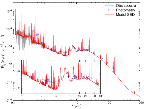
Figure 6: Comparison of the observations (grey lines and blue circles) with the model SED by our Cloudy fitting in the range of $0.1-1000$ µm. We scaled the de-reddened flux density of the observed spectra to match with broadband flux densities of the entire nebula listed in Table A2 and $I$(He ii 1640 Å) of 5.23(–11) erg s^-1 cm^-2 for the IUE spectrum. The inset displays the close-up of $1-40$ µm SED.

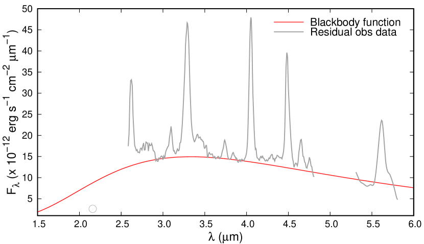
Figure 7: Near-IR excess and the blackbody fitting. The grey lines/circle are the residual flux density between the observed AKARI/IRC and Spitzer/IRS spectra and WFCAM $K$ photometry and the corresponding values obtained from the Cloudy model. The red line is the best fit of this near-IR excess with a blackbody function with a single temperature of $870~{}\pm~{}20$ K.

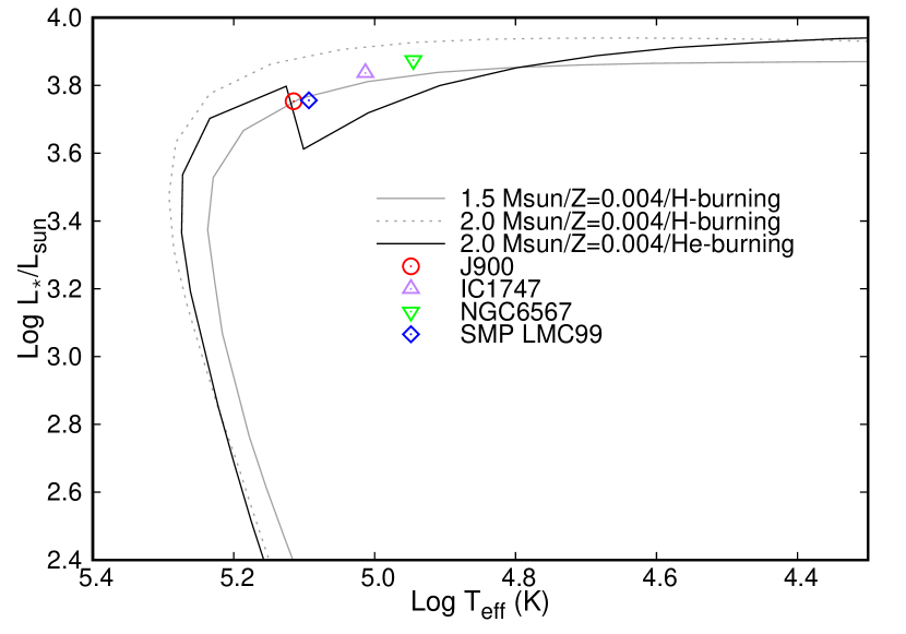
Figure 8: The location of the CSPN of J900 (red circle) on the post-AGB H-shell and He-shell burning tracks. For comparisons, we plot the location of PNe, IC1747, NGC6567, and SMP LMC99 (see § 5). See text for details.

The input parameters and the derived physical quantities are summarised in Tables 6, 8, and 9. The observed and model predicted line fluxes and band fluxes/flux densities are compared in Appendix Table 7 (reduced-$\chi^{2}$ of 27 in the best model). We try to reproduce the observed H₂ line fluxes at 6.91/9.68/12.28 µm. From such efforts, we have found a reasonable temperature floor from the best-fitting model (829 K), which is close to the empirically derived $T$(H₂) = $755~{}\pm~{}36$ K in the case of fitting towards the above three H₂ lines (see § 3.4). The best-fitting model predicts the H₂ 6.91, 9.68, and 12.28 µm line fluxes of 0.555, 0.768, and 0.128 with respect to $I$(H$\beta$) = 100, respectively. Our model succeeds in reproducing H₂ in the mid-IR, which is the majority of the molecular gas mass. Due to such a high floor temperature for CO lines, the predicted $N$(CO) is far from the estimated $N$(CO) by Huggins et al. (1996) (Table 9). Fitting the observationally estimated $N$(CO) requires a lower floor temperature, accordingly causing lower H₂ 6.91/9.68 µm line fluxes and higher $N$(H₂). However, we should take into account that the upper limit of $N$(CO) by Huggins et al. (1996) might be too large because their estimate was done using a no-constrained temperature range ($7-77$ K) and the uncertain CO $J=2-1$ line flux only. The predicted radial profiles of $N$(C) and $N$(CO) (not presented here) indicate that CO seems to be largely not disassociated. The currently best-fitting model can be revised by detecting more CO lines and other molecular gas lines in future observations.

Our model fairly well reproduces the empirically determined $\epsilon$(X) (Table 7), except for Mg & Si. The predicted $\epsilon$(Mg,Si) values are 7.08 and 5.97, whereas those empirically determined values were $7.35~{}\pm~{}0.06$ and $6.97~{}\pm~{}0.14$, respectively (Table 4). The discrepancy of $\epsilon$(Mg) may come from the ICF(Mg) (3.34 in the model vs. $7.28~{}\pm~{}1.02$ in the empirical method). By applying the model predicted ICF(Mg) to the empirically determined Mg^3+,4+, we obtain $\epsilon$(Mg) = $7.35-\log\,(7.35/3.34)$ = 7.01. The large discrepancy of $\epsilon$(Si) must be caused by the line emissivity of [Si ii] 34.8 µm which is peaked in the neutral gas regions beyond the ionisation front (i.e., $R>3.5^{\prime\prime}$). In $\epsilon$(Si) estimation, we assumed that the S/S⁺ and Si/Si⁺ ratios are comparable. However, this assumption is irrelevant as the model predicts that S/S⁺ and Si/Si⁺ ratios are 8.49 and 4.59, respectively. Along with $T_{\rm e}$([O i]) and $n_{\rm e}$([N i]) for $\epsilon$(Si) and ICF(Si) = 4.59 from the model, we obtain a slightly improved $\epsilon$(Si) = $6.24~{}\pm~{}0.07$. We will avoid any further discussion for the Si abundance since it involves various uncertainty.

The modelled SED (red line) displays a reasonable fit to the observed one (grey lines and blue circles, Fig. 6) except for the $\sim$$2-5$ µm SED (inset of Fig. 6), where the observed SED substantially exceeds the modelled one. In Fig. 7, we show the residual flux density between the observed and the corresponding predicted SEDs. The NIR-excess as seen in Fig. 7 is clearly broad and is not due to the emission of H₂, PAH, and atomic gas.

The NIR-excess SED in J900 was firstly suggested by Zhang & Kwok (1991). This near-IR (NIR) excess can be reproduced by an approximate luminosity of 85 L_☉ from the gas shell radius of 19 AU (0.003^′′) with a single blackbody temperature of $870~{}\pm~{}20$ K. Therefore, the NIR-excess would be due to either (i) thermal radiation from very small dust grains or (ii) normal-sized dust grains in substructures surrounding the CSPN (e.g., disc). We rule out the former possibility; as the heat capacity in small-sized grains is smaller than that in large ones, small-sized grains distributed nearby the central star would heat up over the grain sublimation temperature (1750 K) by the central star radiation. We confirmed this in a test model including AC grains with $a<0.005$ $\mu$m. The estimated emitting radius seems to support the latter possibility.

In Fig. 8, we plot the derived luminosity ($L_{\ast}$) and $T_{\rm eff}$ of the CSPN on the post-AGB evolutionary tracks. For comparison, we plot the location of the PNe, IC1747, NGC6567, and SMP LMC99, also (see § 5 for details). These plots are used to infer the initial mass of the progenitor star as well as its post-AGB evolution. Here, we select the H-shell burning post-AGB evolutionary track of stars with initial mass 1.5 M_⊙ and 2.0 M_⊙ with $Z=0.004$ by Vassiliadis & Wood (1994). Additionally, we plot a He-shell burning evolutionary track of a star of initial mass 2.0 M_☉ star with $Z=0.004$ generated by a linear extrapolation from the 2.0 M_☉/$Z=0.0016$ and 2.0 M_☉/$Z=0.008$ He-burning models of Vassiliadis & Wood (1994). The location of the CSPN on these tracks indicates that J900 evolved from a star of initial mass of $\sim$1.5-2 M_☉. We will further discuss the origin and evolution of J900 in § 5.

Table 7: Comparison of $\epsilon$(X) determined by our empirical method ($\epsilon$(X)_Emp., see Table 4) and Cloudy best fitting ($\epsilon$(X)_Cloudy). The values in the last column are the difference between them.

X	$\epsilon$(X)Emp.	$\epsilon$(X)Cloudy	$\Delta$($\epsilon$(X)Cloudy – $\epsilon$(X)Emp.)
He	$11.04~{}\pm~{}0.04$	$10.97$	$-0.07$
C	$9.04~{}\pm~{}0.10$	$8.92$	$-0.12$
N	$7.84~{}\pm~{}0.11$	$7.66$	$-0.18$
O	$8.47~{}\pm~{}0.02$	$8.47$	$0.00$
F	$5.16~{}\pm~{}0.07$	$5.03$	$-0.13$
Ne	$7.95~{}\pm~{}0.02$	$7.90$	$-0.05$
Mg	$7.35~{}\pm~{}0.06$	$7.08$	$-0.27$
Si	$6.97~{}\pm~{}0.14$	$5.97$	$-1.00$
P	$5.49~{}\pm~{}0.05$	$5.21$	$-0.28$
S	$6.53~{}\pm~{}0.02$	$6.47$	$-0.06$
Cl	$4.80~{}\pm~{}0.03$	$4.83$	$+0.03$
Ar	$5.95~{}\pm~{}0.02$	$5.89$	$-0.06$
K	$4.44~{}\pm~{}0.07$	$4.28$	$-0.16$
Fe	$5.83~{}\pm~{}0.21$	$5.63$	$-0.20$

Table 8: Nebular mass component in J900.

Gas species	within ionisation front	entire nebula
Ionised atomic (M☉)	2.61(–1)	2.65(–1)
Neutral atomic (M☉)	1.66(–2)	5.48(–1)
Molecules (M☉)	4.52(–4)	1.11(–2)
Total (M☉)	2.78(–1)	8.25(–1)
Dust and PAH species	within ionisation front	entire nebula
AC grains (M☉)	1.43(–4)	4.24(–4)
Ionised PAH (M☉)	8.49(–7)	8.90(–6)
Neutral PAH (M☉)	1.24(–6)	1.29(–5)
Total (M☉)	1.45(–4)	4.46(–4)
GDR	1916	1849

Table 9: Comparison between the model predicted and observed molecular gas column densities. $N$(H₂) is the value of the warm temperature component. $N$(CO) is the empirically determined value by Huggins et al. (1996).

Species X	$\log\,N$(X)(model) (cm-2)	$\log\,N$(X)(obs) (cm-2)
H2	18.94	$19.06~{}\pm~{}0.11$
CO	13.29	$<14.95$

In Table 8, we summarise the nebular mass components and the gas-to-dust mass ratio (GDR) within the ionisation front (i.e., PDRs are excluded; see the second column) and in the entire nebula (i.e., PDRs included; see the third column). The GDR corresponds to the ratio of (total gas mass) to (AC dust + ionised and neutral PAHs). In Table 9, we compare the predicted $N$(H₂) and $N$(CO) with the observed values. To account for the observed H₂ line fluxes, we added regions with a constant $n_{\rm H}=87\,500$ cm^-3 beyond the ionisation front. Therefore, it is not unusual that the majority of the predicted gas mass is a neutral atomic gas component. Similarly, most of the AC grains and PAHs are co-distributed in the neutral atomic/molecular gas-rich PDRs. Note that our model revises previous gas mass and GDR estimates. It is very important that about 67 $\%$ of the total gas and AC grains exists beyond the ionisation front.

In earlier studies, Huggins et al. (1996) estimated the ionised atomic gas mass of 1.1(–2) M_☉ and the molecular gas mass of 4.0(–4) M_☉ using the line flux of the tentative detection of CO $J=2-1$ at 230 GHz and unconstrained CO gas temperature and CO/H₂ mass ratio under $D=1.6$ kpc. Adopting $D=6.0$ kpc, their estimated masses would increase up to 0.15 M_☉ for the ionised atomic gas and 5.63(–3) M_☉ for the molecular gas. However, these values are far from our “total” gas mass estimate (i.e., the sum of the ionised/neutral atomic gas and molecular gas masses) because they did not consider the neutral gas component. Stasińska & Szczerba (1999) derived GDR of 714 which is the ratio of the ionised atomic gas mass to the dust mass. They estimated the dust mass by blackbody SED fitting for the IRAS bands with contributions from components (e.g., atomic gas emission) other than dust continuum, where they excluded the neutral atomic and molecular gas components. If we exclude these two gas components, the GDR would decrease from 1849 to 585 [= 2.61(–1) M_☉/4.46(–4) M_☉], which is comparable with Stasińska & Szczerba (1999).

In short, our model thoroughly revises the previous gas/dust mass and GDR estimates, which allows us to trace the ejected mass from the progenitor of J900. Furthermore, our modelling work implies that we often tend to underestimate the whole mass-loss history of the PN progenitors and GDR as well, when PDRs are excluded. Our model also seems to remind us of the importance of PDRs in understanding stellar mass loss.

5 Discussion

5.1 Comparison with AGB models

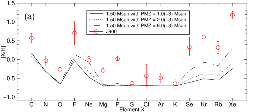
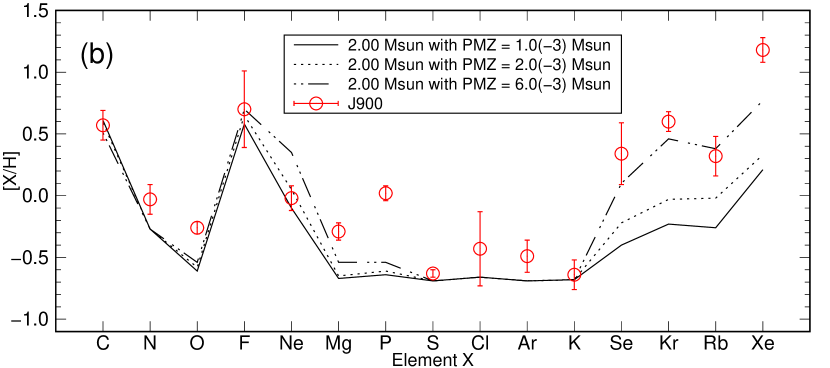
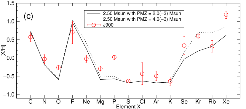
Figure 9: Comparisons between the observed elemental abundances (red circles) and the AGB nucleosynthesis model predictions by Karakas et al. (2018) for stars of initial mass of 1.5, 2.0, and 2.5 M_☉ stars with different partial mixing zone (PMZ) masses. Here, we adopt the empirically determined values listed in column (9) of Table 4.

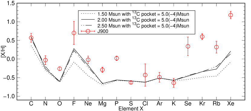
Figure 10: Comparisons between the observed elemental abundances (red circles) and the AGB nucleosynthesis model predictions for tars of initial mass of 1.5, 2.0, and 2.5 M_☉ with $Z=0.003$, which are taken from the FRUITY database (Cristallo et al., 2011; Cristallo et al., 2015). These models adopt the standard ¹³C pocket mass for low mass stars ($\sim$5.0$\times 10^{-4}$ M_☉; Gallino et al., 1998).

Table 10: Elemental abundances of PNe displaying similar abundance patterns to J900. In all the PNe, C abundances are the C CEL values. Se and Kr in IC1747 and NGC6567 are from Sterling et al. (2015). The abundances in IC1747 are the average between Henry et al. (2010) and Wesson et al. (2005). C, N, and Ne in SMP LMC99 are from Leisy & Dennefeld (2006), and the others are taken from Mashburn et al. (2016). $\epsilon$(Se) in J900 is from Sterling et al. (2015).

PN	$\epsilon$(He)	$\epsilon$(C)	$\epsilon$(N)	$\epsilon$(O)	$\epsilon$(F)	$\epsilon$(Ne)	$\epsilon$(S)	$\epsilon$(Cl)	$\epsilon$(Ar)	$\epsilon$(Se)	$\epsilon$(Kr)	$\epsilon$(Rb)	$\epsilon$(Xe)	Ref.
IC1747	11.07	8.98	8.14	8.58	$\cdots$	8.01	6.66	4.98	6.14	3.68	$<4.34$m	$\cdots$	$\cdots$	(1),(2),(3)
NGC6567	11.01	8.74	7.61	8.30	$\cdots$	7.45	6.68	4.75	5.67	3.23	$<3.62$m	$\cdots$	$\cdots$	(3),(4)
SMP LMC99	11.04	8.69	8.15	8.42	$\cdots$	7.62	6.42	$\cdots$	5.95	3.56	3.78	$<2.62$m	$\cdots$	(5),(6)
J900	11.04	9.04	7.84	8.47	5.16	7.95	6.53	4.80	5.95	3.65	3.85	2.86	3.42	(3),(7)

References –

(1) Henry et al. (2010); (2) Wesson et al. (2005); (3) Sterling et al. (2015); (4) Hyung et al. (1993); (5) Leisy & Dennefeld (2006); (6) Mashburn et al. (2016); (7) This work.

In order to verify and further constrain the evolution of the progenitor star, then, we compare the observed and the AGB model predicted $\epsilon$(X). Here, we select the AGB nucleosynthesis models of Karakas et al. (2018) for the initially 1.5, 2.0, and 2.5 M_☉ stars with $Z=0.003$. The models of Karakas et al. (2018) artificially add a partial mixing zone (PMZ) at the bottom of the convective envelope during each TDU. At the PMZ, protons from the H-envelope are mixed into the He-intershell and then captured by ¹²C. Thus, ¹³C pocket as an extra $n$-source is formed. In Fig. 9(a) to (c), we plot the observed (red circles with an error bar) and the model predicted abundances (lines and dots). As Karakas et al. (2018) use the scaled solar abundance of Asplund et al. (2009) as the initial abundance, we adopt the empirically determined values listed in the column (9) of Table 4 (i.e, [X/H]_AS). It should be noted that empirically determined $\epsilon$(Mg) would be overestimated as we explained in § 4.2; adopting the Cloudy model predicted ICF(Mg), we obtain [Mg/H]_AS = $-0.63~{}\pm~{}0.07$ whose value is in agreement with the AGB model predicted values. In these plots, we find that (1) C, F, Ne, and $n$-capture elements increase as the initial mass is greater, (2) F production is more sensitive to the initial mass than C and Ne productions, and (3) Ne production is sensitive to both the initial mass of the progenitor star and the PMZ mass. It is the most important finding that all the observed $n$-capture elemental abundances cannot be explained without PMZ masses and their yields are in large dependence of PMZ mass. Thus, the C¹³ pocket is certainly formed in the progenitor star. Either the 2.0 M_☉ model with PMZ $=6.0(-3)$ M_☉ or the 2.5 M_☉ model with PMZ $=4.0(-3)$ M_☉ are in excellent accordance with the observed $\epsilon$(X). The enhancement of Ne is related to ²²Ne, which is formed via the double $\alpha$ capturing by ¹⁴N in ¹³C pocket. In $\geq 2.5$ M_⊙ models, the He-shell temperature exceeds 300M K required to activate the ²²Ne($\alpha$,$n$)²⁵Mg reaction during the last few TPs (see their Fig. 5 of Karakas et al., 2018). Consequently, as suggested in van Raai et al. (2012), high $n$ density produces more Rb over Kr as seen in Fig. 9(c). From the comparison between the observed and predicted [Rb/Kr], we infer the initial mass to be $<2.5$ M_☉. The derived gas mass (0.838 M_☉, Table 8) and the range of the CSPN mass ($0.64-0.69$ M_☉; Vassiliadis & Wood, 1994), the progenitor is certainly a $>1.5$ M_☉ star.

Note that the observed O abundance in J900 is larger than the predicted O in the models with any PMZ masses. The observed [O/(Cl,Ar)] and $\epsilon$(O,Cl) in J900 are along the result of Delgado-Inglada et al. (2015), who demonstrated that O in C-rich PNe is enhanced by $\sim$0.3 dex in their plots of O/Cl versus $\epsilon$(O) and $\epsilon$(Cl). For an explanation of the O enhancement in C-rich PNe, Delgado-Inglada et al. (2015) proposed a convective overshooting, which is not considered in the AGB models of Karakas et al. (2018).

There are several other AGB nucleosynthesis models. Of these, we compare the observed abundances with the predictions by the FRUITY models (Cristallo et al., 2011; Cristallo et al., 2015) as presented in Fig. 10. These models adopt the standard ¹³C pocket mass ($\sim$5$\times 10^{-4}$ M_☉; Gallino et al., 1998). Clearly, any FRUITY models fail to explain the observed $n$-capture elements, owing to low ¹³C pocket mass. Thus, we realise the importance of the PMZ/¹³C pocket in the production of these elements.

The evolutionary age of the progenitors does not make much difference, whether or not the progenitor experienced H-burning (i.e., evolving to H-rich WD) or He-burning (i.e., to H-poor WD) after the AGB phase. We estimate the current age of the progenitor to be $\sim$$1.2$ Gyr for a star of initial mass of 2.0 M_☉ (or $\sim$$0.6$ Gyr for 2.5 M_☉) with $Z=0.004$ by referring to the H-burning post-AGB evolutionary tracks of Vassiliadis & Wood (1994). Our estimate is largely different from Stanghellini & Haywood (2018), who classified J900 as the older population with its age of $>7.5$ Gyr in terms of C and N enhancements only.

We summarise this section as follows. We compare the observed 15 elemental abundances with AGB model predictions. As a result, we derive the current evolutionary status of the CSPN. J900 is a young C-rich PN together with large enhancements of F and $n$-capture elements, and it evolved from a star of initial mass of $\sim$2.0 M_☉ formed in a low-metallicity environment ($Z\sim 0.003$).

5.2 Comparison with other PNe

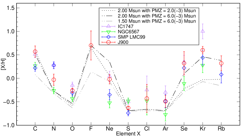
Figure 11: Comparisons between the observed elemental abundances of PNe (Table 10) and the AGB nucleosynthesis model predictions by Karakas et al. (2018) for stars of initial mass of 1.5 and 2.0 M_☉ with different PMZ masses.

We compare J900 with PNe IC1747 and NGC6567 in the Milky Way and SMP LMC99 in the Large Magellanic Cloud in order to examine the validity of our derived abundances and the possible range of the PMZ mass in J900. We select these PNe because their abundances are very similar to J900, and $n$-capture elements are already measured (Table 10).

In Fig. 8, we plot their $T_{\rm eff}$ and $L_{\ast}$ on the post-AGB evolutionary tracks in order to check the current evolutionary status and the initial mass of these three PNe. The respective $T_{\rm eff}$ values are 103 090 K in IC1747 and 88 130 K in NGC6567, which are derived using the observed $I$(He ii 4686 Å)/$I$(H$\beta$) ratio and the equation (3.1) of Dopita & Meatheringham (1991). In the $L_{\ast}$ calculations for IC1747 (6860 L_☉) and NGC6567 (7490 L_☉), we utilise the stellar atmosphere model of Rauch (2003) with the derived $T_{\rm eff}$, $\log\,g$ = 5.0 cm s^-2, [Z/H] = –0.5, and the following parameters: (1) For IC1747, $D$ = 3.24 kpc (from GAIA parallax; Gaia Collaboration et al., 2018), $m_{V}$ of the CSPN (16.4; Tylenda et al., 1991), and c(H$\beta$) = 1.00 (Wesson et al., 2005); (2) For NGC6567, $D$ = 2.4 kpc (Phillips, 2004), HST NICMOS1 $F_{\lambda}$ of 6.42(–12) erg s^-1 cm^-2 µm^-1 at the F108N band ($\lambda_{\rm c}=1.082$ µm), and c(H$\beta$) = 0.68 (Hyung et al., 1993). $T_{\rm eff}$ and $L_{\ast}$ of LMC99 (124 000 K and 5700 L_☉) are taken from Dopita & Meatheringham (1991).

The transition from the AGB to the PN involves stellar mass loss, involving a stellar wind change from a slow to a fast speed. During this transition period, the central star might experience the He-burning phase, responsible for the presently derived abundances. As seen in Fig. 8, all the CSPN temperatures are presently increasing (not yet cooling down) along the post-AGB tracks toward higher temperature values. The locations seem to indicate that these PNe presumably originated from similar initial mass stars and exited the AGB phase a fairly long ago. Thus, we can safely compare their abundances with the theoretical predictions of Karakas et al. (2018) for the initially $1.5-2.0$ M_☉ stars.

In Fig. 11, we plot the observed and the model-predicted abundances. For IC1747, NGC6567, and LMC99, we adopt the uncertainty of 0.05 dex for $\epsilon$(C/N/O/Ne/S/Cl/Ar) and 0.15 dex for $\epsilon$(Se/Kr/Rb), respectively. We find the following results: (1) [C,Ne/H] indicates that J900 and IC1747 evolved from the initially 2.0 M_☉ stars as described in § 5.1, and (2) NGC6567 and LMC99 from the stars whose initial mass could be between 1.5 and 2.0 M_☉. Meanwhile, (3) [Se,Kr,Rb] suggests that all of these PNe are descendants of 2.0 M_☉ stars. As seen in the case of J900 (and see Fig. 9(c)), [Kr/Rb] $<0$ in LMC99 suggests that the initial mass of this PN does not exceed 2.5 M_☉.

Although there is a slight indeterminacy in the initial mass, all of these PNe show very similar abundance patterns, which can be adequately explained by either 1.5 M_☉ or 2.0 M_☉ models. Based on the self-consistent model for the observables, we confirm that (1) the derived elemental abundances of J900 are not peculiar and but quite similar to IC1747, NGC6567, and LMC99; (2) PMZ mass would be $(2.0-6.0)\times 10^{-3}$ M_☉ required to match with the observed abundances of all of these PNe; and (3) the initial masses predicted from elemental abundances are consistent with those deduced from the locations on the post-AGB evolution tracks.

6 Summary

We performed detailed spectroscopic analyses of J900 in order to characterise the properties of the CSPN and nebula. We obtained 17 elemental abundances. J900 is a C, F, and $n$-capture element rich PN. We investigated the physical conditions of H₂. The H₂ lines are likely to be emitted from the warm ($\sim$670 K) and hot ($\sim$3200 K) temperature regions. We constructed the SED model to be consistent with all the observed quantities of the CSPN and the dusty nebula. We found that about 67 % of the total dust and gas components exist beyond the ionisation front, indicating the presence of the neutral atomic and molecular gas-rich PDRs, critically important in the understanding of the stellar mass loss and also the recycling of galactic material. The best-fitting SED shows an excellent agreement with the observations except for the observed near-IR SED. The near-IR excess suggests the presence of a high-density structure near the central star. The best-fitting SED model indicates that the progenitor evolved from a star of initial mass $\sim$2.0 M_☉ had been in the course of the He-burning phase after AGB. The present age is likely to be $\sim$1 Gyr after the progenitor star was formed. The derived elemental abundance pattern is consistent with that predicted by the AGB nucleosynthesis model for 2.0 M_☉ stars with $Z=0.003$ and a PMZ $=6.0(-3)$ M_☉. Other models without PMZ cannot accommodate the observed abundances of $n$-capture elements, strongly suggesting that the ¹³C pocket is likely to be formed in the He-intershell of the progenitor. We showed how critically important the physical properties of the CSPN and the nebula derived through multiwavelength data analysis are for understanding the origin (i.e., initial mass and age) and internal evolution of the PN progenitors. Accurately determined abundances (in particular, C/F/Ne/$n$-capture elements) and gas/dust masses are very helpful for these purposes.

Appendix A Supporting Results

Table A11: Identified emission lines in J900.

$\lambda_{\rm lab.}$ (Å)	Line	$f(\lambda)$	$I$($\lambda$)	$\delta$ $I$($\lambda$)	$\lambda_{\rm lab.}$ (Å)	Line	$f(\lambda)$	$I$($\lambda$)	$\delta$ $I$($\lambda$)	$\lambda_{\rm lab.}$ (Å)	Line	$f(\lambda)$	$I$($\lambda$)	$\delta$ $I$($\lambda$)
1548/51	C iv	$1.238$	624.365	13.594	$5047.74$	He i	$-0.048$	0.134	0.010	$7135.80$	[Ar iii]	$-0.374$	8.470	0.173
$1640.42$	He ii	$1.177$	235.081	4.276	$5191.82$	[Ar iii]	$-0.081$	0.084	0.006	$7170.50$	[Ar iv]	$-0.378$	0.086	0.003
1749/54	N iii]	$1.154$	19.214	5.870	$5197.90$	[N i]	$-0.082$	0.345	0.009	$7177.50$	He ii	$-0.379$	0.395	0.009
1906/09	C iii]	$1.258$	1026.996	22.841	$5200.26$	[N i]	$-0.083$	0.257	0.008	$7236.42$	C ii	$-0.387$	0.414	0.012
2325/26/28	[C ii]	$1.372$	87.207	3.980	$5342.43$	C ii	$-0.112$	0.056	0.009	$7262.70$	[Ar iv]	$-0.391$	0.070	0.004
2422/25	[Ne iv]	$1.127$	48.638	1.998	$5355.87$	[Fe iii]	$-0.115$	0.033	0.004	$7281.35$	He i	$-0.393$	0.639	0.015
$2733.30$	He ii	$0.720$	7.631	0.725	$5411.52$	He ii	$-0.126$	2.785	0.029	$7318.92$	[O ii]	$-0.398$	5.782	0.099
$3721.94$	H i	$0.323$	2.750	0.387	$5470.68$	C iv	$-0.137$	0.057	0.005	$7329.66$	[O ii]	$-0.400$	5.022	0.111
$3726.03$	[O ii]	$0.322$	75.920	1.385	$5480.96$	Fe ii	$-0.139$	0.032	0.002	$7486.80$	C iii	$-0.421$	0.020	0.002
$3728.81$	[O ii]	$0.322$	42.811	1.403	$5483.35$	C ii	$-0.139$	0.021	0.002	$7499.85$	He i	$-0.422$	0.040	0.003
$3734.37$	H i	$0.321$	2.969	0.176	$5517.72$	[Cl iii]	$-0.145$	0.298	0.008	$7530.80$	[Cl iv]	$-0.426$	0.180	0.005
$3750.15$	H i	$0.317$	2.532	0.277	$5519.53$	Fe iii	$-0.145$	0.035	0.005	$7534.88$	Ca i	$-0.427$	0.041	0.004
$3759.87$	O iii	$0.315$	3.154	0.189	$5537.89$	[Cl iii]	$-0.149$	0.436	0.007	$7722.58$	Mg i]	$-0.452$	0.011	0.001
$3770.63$	H i	$0.313$	3.439	0.164	$5577.34$	[O i]	$-0.156$	0.111	0.007	$7725.00$	N ii	$-0.452$	0.019	0.003
$3797.90$	H i	$0.307$	5.243	0.192	$5592.25$	O iii	$-0.158$	0.054	0.005	$7725.90$	C iv	$-0.452$	0.241	0.007
$3835.38$	H i	$0.299$	7.654	0.183	$5709.11$	[Xe iv]	$-0.177$	0.030	0.006	$7736.00$	C iv	$-0.453$	0.026	0.002
$3868.76$	[Ne iii]	$0.291$	117.595	2.176	$5710.77$	N ii	$-0.178$	0.061	0.004	$7751.10$	[Ar iii]	$-0.455$	2.069	0.052
$3889.05$	H i	$0.286$	19.620	0.356	$5754.64$	[N ii]	$-0.185$	1.243	0.015	$7816.13$	He i	$-0.464$	0.044	0.004
$3964.73$	He i	$0.267$	0.610	0.064	$5759.43$	He iia	$-0.185$	0.006	0.002	$7875.99$	[P ii]	$-0.471$	0.067	0.004
$3967.47$	[Ne iii]	$0.267$	35.354	0.622	$5759.64$	[Rb iv]	$-0.185$	0.014	0.004	$8113.58$	P iii	$-0.501$	0.052	0.002
$3970.07$	H i	$0.266$	17.820	0.279	$5801.33$	C iv	$-0.192$	0.310	0.007	$8236.79$	He ii	$-0.515$	0.752	0.022
$4025.60$	He ii	$0.251$	0.520	0.070	$5811.97$	C iv	$-0.193$	0.160	0.007	$8247.73$	H i	$-0.516$	0.049	0.006
$4026.20$	He i	$0.251$	1.936	0.081	$5846.66$	He iib	$-0.199$	0.014	0.004	$8249.97$	H i	$-0.517$	0.061	0.010
$4045.70$	Ca i	$0.246$	0.456	0.042	$5846.67$	[Xe iii]	$-0.199$	0.024	0.007	$8252.40$	H i	$-0.517$	0.072	0.007
$4059.90$	[F iv]	$0.241$	0.072	0.014	$5857.26$	He ii	$-0.200$	0.015	0.004	$8260.93$	H i	$-0.518$	0.031	0.004
$4060.20$	N ii	$0.241$	0.129	0.021	$5867.74$	[Kr iv]	$-0.202$	0.146	0.005	$8262.33$	Ca i	$-0.518$	0.027	0.004
$4067.94$	C iii	$0.239$	0.492	0.116	$5875.62$	He i	$-0.203$	11.723	0.135	$8264.28$	H i	$-0.518$	0.063	0.005
$4068.60$	[S ii]	$0.239$	1.961	0.164	$5913.26$	He ii	$-0.209$	0.022	0.003	$8267.94$	H i	$-0.519$	0.064	0.004
$4070.31$	C iii	$0.239$	0.537	0.049	$5931.83$	He ii	$-0.211$	0.057	0.004	$8271.93$	H i	$-0.519$	0.049	0.004
$4076.35$	[S ii]	$0.237$	0.823	0.065	$5977.03$	He ii	$-0.218$	0.040	0.004	$8276.31$	H i	$-0.520$	0.088	0.006
$4089.29$	O ii	$0.233$	0.095	0.032	$6004.72$	He ii	$-0.222$	0.056	0.006	$8281.12$	H i	$-0.520$	0.093	0.005
$4097.38$	N ii	$0.231$	0.712	0.028	$6036.78$	He ii	$-0.226$	0.063	0.002	$8292.31$	H i	$-0.521$	0.067	0.003
$4101.73$	H i	$0.230$	29.172	0.415	$6074.19$	He ii	$-0.232$	0.079	0.003	$8298.83$	H i	$-0.522$	0.096	0.004
$4120.81$	He i	$0.224$	0.292	0.039	$6086.99$	Fe i?	$-0.233$	0.022	0.003	$8306.11$	H i	$-0.523$	0.120	0.004
$4128.66$	N ii	$0.222$	0.143	0.017	$6101.79$	[K iv]	$-0.235$	0.115	0.004	$8312.10$	C iii	$-0.524$	0.056	0.003
$4143.76$	He i	$0.217$	0.285	0.024	$6118.26$	He ii	$-0.238$	0.083	0.003	$8314.26$	H i	$-0.524$	0.116	0.004
$4189.79$	O ii	$0.204$	0.491	0.035	$6151.27$	C ii	$-0.242$	0.049	0.005	$8323.42$	H i	$-0.525$	0.145	0.005
$4199.83$	He ii	$0.200$	0.847	0.032	$6159.89$	Fe iii?	$-0.243$	0.129	0.006	$8333.78$	H i	$-0.526$	0.189	0.007
$4238.29$	C iii	$0.189$	0.129	0.018	$6170.60$	He ii	$-0.245$	0.084	0.004	$8342.20$	C iii	$-0.527$	0.040	0.002
$4254.12$	O ii	$0.184$	0.085	0.016	$6174.94$	[Br iv]?	$-0.246$	0.016	0.002	$8345.47$	H i	$-0.527$	0.158	0.005
$4267.18$	C ii	$0.180$	1.183	0.035	$6209.27$	Ca i	$-0.250$	0.018	0.001	$8359.00$	H i	$-0.529$	0.196	0.006
$4338.67$	He ii	$0.157$	0.964	0.018	$6233.82$	He ii	$-0.254$	0.113	0.005	$8361.73$	He i	$-0.529$	0.071	0.003
$4340.46$	H i	$0.157$	49.523	0.434	$6238.39$	Fe ii	$-0.254$	0.013	0.002	$8374.48$	H i	$-0.531$	0.201	0.006
$4363.21$	[O iii]	$0.149$	14.442	0.218	$6256.52$	C ii	$-0.257$	0.021	0.002	$8386.40$	N iii	$-0.532$	0.017	0.003
$4387.93$	He i	$0.142$	0.566	0.023	$6257.62$	O i	$-0.257$	0.015	0.002	$8392.40$	H i	$-0.533$	0.239	0.008
$4471.47$	He i	$0.115$	3.799	0.033	$6300.30$	[O i]	$-0.263$	7.974	0.358	$8413.32$	H i	$-0.535$	0.271	0.009
$4541.59$	He ii	$0.093$	1.250	0.015	$6310.80$	He ii	$-0.264$	0.125	0.010	$8437.95$	H i	$-0.537$	0.331	0.010
$4571.10$	Mg i]	$0.084$	0.323	0.018	$6312.10$	[S iii]	$-0.264$	1.249	0.019	$8446.48$	O i	$-0.538$	0.080	0.004
$4634.12$	N iii	$0.065$	0.426	0.016	$6363.78$	[O i]	$-0.271$	2.742	0.042	$8467.25$	H i	$-0.541$	0.404	0.012
$4640.64$	N iii	$0.063$	0.950	0.015	$6406.38$	He ii	$-0.277$	0.156	0.004	$8480.79$	He i	$-0.542$	0.017	0.002
$4641.81$	O ii	$0.063$	0.137	0.010	$6434.73$	[Ar v]	$-0.281$	0.207	0.008	$8502.48$	H i	$-0.544$	0.424	0.013
$4647.42$	C iii	$0.061$	0.458	0.011	$6461.95$	C ii	$-0.284$	0.103	0.003	$8519.35$	He ii	$-0.546$	0.028	0.003
$4649.13$	O ii	$0.061$	0.080	0.010	$6471.66$	Ca i	$-0.285$	0.169	0.005	$8541.88$	He ii	$-0.548$	0.044	0.007
$4650.25$	C iii	$0.060$	0.296	0.015	$6515.90$	N iii	$-0.291$	0.037	0.003	$8545.38$	H i	$-0.549$	0.556	0.017
$4651.47$	C iii	$0.060$	0.120	0.014	$6527.24$	[N ii]	$-0.293$	0.207	0.005	$8578.69$	[Cl ii]	$-0.552$	0.139	0.005
$4658.05$	[Fe iii]	$0.058$	0.184	0.012	$6548.04$	[N ii]	$-0.296$	17.678	0.709	$8582.61$	He i	$-0.552$	0.050	0.005
$4658.30$	C iv	$0.058$	0.487	0.014	$6560.00$	He ii	$-0.297$	5.875	0.691	$8598.39$	H i	$-0.554$	0.674	0.020
$4685.71$	He ii	$0.050$	35.847	0.173	$6562.80$	H i	$-0.298$	286.007	4.772	$8616.59$	Ca i	$-0.556$	0.070	0.005
$4711.37$	[Ar iv]	$0.042$	1.866	0.025	$6578.05$	C ii	$-0.300$	0.453	0.014	$8626.19$	He ii	$-0.557$	0.030	0.003
$4713.14$	He i	$0.042$	0.582	0.020	$6583.46$	[N ii]	$-0.300$	53.335	0.902	$8665.02$	H i	$-0.560$	0.858	0.026
$4714.17$	[Ne iv]	$0.041$	0.195	0.018	$6656.00$	Fe ii]	$-0.310$	0.145	0.004	$8727.12$	[C i]	$-0.566$	0.241	0.010
$4715.61$	[Ne iv]	$0.041$	0.074	0.010	$6678.15$	He i	$-0.313$	3.127	0.053	$8746.89$	He ii	$-0.568$	0.024	0.004
$4724.17$	[Ne iv]	$0.038$	0.202	0.009	$6683.20$	He ii	$-0.313$	0.262	0.009	$8750.47$	H i	$-0.568$	1.072	0.033
$4725.64$	[Ne iv]	$0.038$	0.158	0.009	$6716.44$	[S ii]	$-0.318$	3.263	0.058	$8845.37$	He i	$-0.576$	0.042	0.004
$4740.16$	[Ar iv]	$0.034$	2.124	0.028	$6730.81$	[S ii]	$-0.320$	5.588	0.100	$8859.15$	He ii	$-0.578$	0.043	0.007
$4751.59$	[Fe iii]	$0.030$	0.069	0.009	$6744.10$	He i	$-0.322$	0.028	0.002	$8862.78$	H i	$-0.578$	1.350	0.042
$4760.87$	O i	$0.001$	2.160	0.116	$6779.94$	C ii	$-0.326$	0.051	0.003	$8929.11$	He ii	$-0.583$	0.041	0.003
$4861.33$	H i	$0.000$	100.000	0.381	$6791.47$	C ii	$-0.328$	0.027	0.003	$9011.21$	He ii	$-0.590$	0.014	0.010
$4906.83$	O ii	$-0.012$	0.157	0.010	$6795.10$	[K iv]	$-0.328$	0.031	0.002	$9014.91$	H i	$-0.590$	0.323	0.017
$4921.93$	He i	$-0.016$	1.018	0.013	$6821.16$	[Mn iii]	$-0.332$	0.009	0.002	$9068.60$	[S iii]	$-0.594$	11.272	0.307
$4931.23$	[O iii]	$-0.019$	0.126	0.008	$6826.70$	[Kr iii]	$-0.333$	0.026	0.006	$9108.54$	He ii	$-0.597$	0.056	0.003
$4959.00$	[O iii]	$-0.026$	357.906	3.090	$7062.28$	He i	$-0.364$	0.079	0.003	$9123.60$	[Cl ii]	$-0.598$	0.040	0.003
$5007.00$	[O iii]	$-0.038$	1048.258	6.313	$7065.71$	He i	$-0.364$	5.210	0.105	$9210.34$	He i	$-0.604$	0.067	0.006
$5015.68$	He i	$-0.040$	1.429	0.012	$7099.80$	[Pb ii]?	$-0.369$	0.037	0.004

Table A1: Continued.

$\lambda_{\rm lab.}$ (µm)	Line		$I$($\lambda$)	$\delta$ $I$($\lambda$)
$3.04$	H i 5-10		0.328	0.070
$3.10$	He ii		1.028	0.056
$3.74$	H i 5-8		0.970	0.082
$3.84$	H2 $v=0-0$ S(13)		0.215	0.057
$4.05$	H i 4-5		7.781	0.107
$4.49$	[Mg iv]		6.128	0.147
$4.65$	H i 5-7		1.147	0.141
$5.61$	[Mg v]		4.509	0.524
$6.91$	H2 $v=0-0$ S(5)		0.762	0.312
$6.98$	[Ar ii]		0.867	0.221
$8.99$	[Ar iii]		6.293	0.903
$9.68$	H2 $v=0-0$ S(3)		1.017	0.220
$10.51$	[S iv]		58.937	3.466
$11.76$	[Cl iv]		0.418	0.042
$12.28$	H2 $v=0-0$ S(2)		0.189	0.057
$12.37$	H i		1.043	0.043
$12.82$	[Ne ii]		4.006	0.249
$13.10$	[Ar v]		1.684	0.118
$13.43$	[F v]		0.309	0.023
$13.52$	[Mg v]		0.370	0.026
$14.07$	He i?		0.362	0.048
$14.32$	[Ne v]		44.563	2.690
$15.56$	[Ne iii]		113.924	6.646
$17.62$	H i?		1.356	0.096
$17.89$	[P iii]		0.724	0.074
$18.72$	[S iii]		15.049	0.890
$19.07$	H i 7-8		0.522	0.102
$20.31$	[Cl iv]		0.307	0.026
$21.83$	[Ar iii]		0.566	0.052
$22.34$	[Fe ii]		0.602	0.047
$24.32$	[Ne v]		25.480	1.491
$25.90$	[O iv]		282.948	16.450
$33.49$	[S iii]		5.215	0.319
$34.84$	[Si ii]		1.427	0.190
$36.02$	[Ne iii]		6.710	0.429

• A predicted $I$(He ii 5759.64 Å) is estimated to be $0.006~{}\pm~{}0.002$ using the theoretical He ii $I$(5759 Å)/$I$(5857 Å) = 0.390 by Storey & Hummer (1995) under Case B assumption.

• A predicted $I$(He ii 5846 Å) is estimated to be $0.014~{}\pm~{}0.004$ using the theoretical He ii $I$(5846 Å)/$I$(5857 Å) = 0.914 by Storey & Hummer (1995) under Case B assumption.

Table A2: Broadband flux density of J900. We assume 3 $\%$ uncertainty because $MSX$ data do not give uncertainty.

$\lambda_{\rm c}$ (µm)	Band	$I_{\lambda}$ (erg s-1 cm-2 µm-1)
$0.4640$	WFC/$g$	$1.17(-8)~{}~{}~{}\pm~{}7.69(-11)$
$0.6122$	WFC/$R$	$2.97(-9)~{}~{}~{}\pm~{}3.98(-11)$
$0.5443$	$HST$/F555W (CSPN)	$6.98(-12)~{}\pm~{}4.57(-13)$
$0.5443$	$HST$/F555W	$1.96(-9)~{}~{}~{}\pm~{}1.48(-11)$
$1.2350$	WFCAM/$J$	$9.92(-11)~{}\pm~{}4.03(-12)$
$1.6620$	WFCAM/$H$	$4.10(-11)~{}\pm~{}1.90(-12)$
$2.1590$	WFCAM/$K$	$4.20(-11)~{}\pm~{}2.06(-12)$
$3.3526$	$WISE$/W1	$3.39(-11)~{}\pm~{}1.75(-12)$
$4.6028$	$WISE$/W2	$2.55(-11)~{}\pm~{}1.38(-12)$
$9.0000$	$AKARI$/S9W	$5.43(-11)~{}\pm~{}3.05(-12)$
$11.5608$	$WISE$/W3	$4.60(-11)~{}\pm~{}2.48(-12)$
$12.1300$	$MSX$/C	$4.70(-11)~{}\pm~{}1.41(-12)$
$14.6500$	$MSX$/D	$4.82(-11)~{}\pm~{}1.45(-12)$
$18.0000$	$AKARI$/L18W	$4.61(-11)~{}\pm~{}2.52(-12)$
$21.3400$	$MSX$/E	$4.03(-11)~{}\pm~{}1.21(-12)$
$22.0883$	$WISE$/W4	$4.85(-11)~{}\pm~{}2.61(-12)$
$65.0000$	$AKARI$/N60	$3.95(-12)~{}\pm~{}5.44(-13)$
$90.0000$	$AKARI$/WIDE-S	$1.55(-12)~{}\pm~{}1.28(-13)$
$140.0000$	$AKARI$/WIDE-L	$4.50(-13)~{}\pm~{}1.73(-13)$
$\nu_{\rm c}$ (GHz)		$F_{\nu}$ (Jy)
$43.0$		$0.090~{}\pm~{}0.020$
$30.0$		$0.086~{}\pm~{}0.005$
$20.0$		$0.119~{}\pm~{}0.012$
$6.0$		$0.109~{}\pm~{}0.011$
$5.0$		$0.121~{}\pm~{}0.036$
$2.7$		$0.180~{}\pm~{}0.060$
$1.4$		$0.108~{}\pm~{}0.022$

Table A3: Atomic data adopted in CEL analysis of J900.

Line	transition probability $A_{ji}$	effective collision strength $\Psi(T)$
$[$C i$]$	Froese Fischer & Saha (1985)	Johnson et al. (1987); Pequignot & Aldrovandi (1976)
$[$C ii$]$	Nussbaumer & Storey (1981); Froese Fischer (1994)	Blum & Pradhan (1992)
C iii$]$	Wiese et al. (1996)	Berrington et al. (1985)
C iv	Wiese et al. (1996)	Badnell & Griffin (2000); Martin et al. (1993)
[N i]	Wiese et al. (1996)	Pequignot & Aldrovandi (1976); Dopita et al. (1976)
[N ii]	Wiese et al. (1996)	Lennon & Burke (1994)
N iii]	Wiese et al. (1996)	Blum & Pradhan (1992)
[O i]	Wiese et al. (1996)	Bhatia & Kastner (1995)
[O ii]	Wiese et al. (1996)	McLaughlin & Bell (1993); Pradhan (1976)
[O iii]	Wiese et al. (1996)	Lennon & Burke (1994)
[O iv]	Wiese et al. (1996)	Blum & Pradhan (1992)
[F iv]	Garstang (1951); Storey & Zeippen (2000)	Lennon & Burke (1994)
[F v]	Rynkun et al. (2012)	Liang et al. (2012)
[Ne ii]	Saraph & Tully (1994)	Saraph & Tully (1994)
[Ne iii]	Mendoza (1983); Kaufman & Sugar (1986)	McLaughlin & Bell (2000)
[Ne iv]	Becker et al. (1989); Bhatia & Kastner (1988)	Ramsbottom et al. (1998)
[Ne v]	Kaufman & Sugar (1986); Bhatia & Doschek (1993)	Lennon & Burke (1994)
[Mg iv]	CHIANTI Data Basea	CHIANTI Data Basea
[Mg v]	Mendoza (1983); Kaufman & Sugar (1986)	Butler & Zeippen (1994)
[Si ii]	Calamai et al. (1993); Bergeson & Lawler (1993); Lanzafame (1994);	Dufton & Kingston (1991)
	Nussbaumer (1977)
[P ii]	Mendoza & Zeippen (1982b)	Tayal (2004a)
[P iii]	Naqvi (1951)	Saraph & Storey (1999)
[S ii]	Verner et al. (1996); Keenan et al. (1993)	Ramsbottom et al. (1996)
[S iii]	Mendoza & Zeippen (1982b); LaJohn & Luke (1993); Kaufman & Sugar (1986);	Galavis et al. (1995)
	Heise et al. (1995)
[S iv]	Johnson et al. (1986); Dufton et al. (1982); Verner et al. (1996)	Dufton et al. (1982)
[Cl ii]	CHIANTI Data Basea	Tayal (2004b)
[Cl iii]	Mendoza & Zeippen (1982a); Kaufman & Sugar (1986)	Ramsbottom et al. (2001)
[Cl iv]	Mendoza & Zeippen (1982b); Ellis & Martinson (1984)	Galavis et al. (1995)
	Kaufman & Sugar (1986)
[Ar iii]	Mendoza (1983); Kaufman & Sugar (1986)	Galavis et al. (1995)
[Ar iv]	Mendoza & Zeippen (1982a); Kaufman & Sugar (1986)	Zeippen et al. (1987)
[Ar v]	Mendoza & Zeippen (1982b); Kaufman & Sugar (1986); LaJohn & Luke (1993)	Galavis et al. (1995)
[K iv]	Mendoza (1983); Kaufman & Sugar (1986)	Galavis et al. (1995)
[Fe iii]	Garstang (1957); Nahar & Pradhan (1996)	Zhang (1996)
[Kr iii]	Biémont & Hansen (1986)	Schoning (1997)
[Kr iv]	Biémont & Hansen (1986)	Schoning (1997)
[Rb iv]	Sterling et al. (2016)	Sterling et al. (2016)
[Xe iii]	Biemont et al. (1995)	Schoening & Butler (1998)
[Xe iv]	Biemont et al. (1995)	Schoening & Butler (1998)

• http://www.chiantidatabase.org

Table A4: Adopted effective recombination coefficient of RLs in analysis of J900.

Line	References
H i	Aller (1984); Storey & Hummer (1995)
He i	Benjamin et al. (1999); Pequignot et al. (1991)
He ii	Benjamin et al. (1999); Storey & Hummer (1995)
C ii	Davey et al. (2000)
C iii, C iv	Pequignot et al. (1991)

Table A5: Adopted $T_{\rm e}$–$n_{\rm e}$ pair for the ionic abundance calculations in J900.

Ion	$T_{\rm e}$ (K)	$n_{\rm e}$ (cm-3)	Ion	$T_{\rm e}$ (K)	$n_{\rm e}$ (cm-3)
He+	$T_{\rm e}$(He i)	10 000	Mg3+	$T_{\rm e}$([Ne iv])	$n_{\rm e}$([Ne v])
He2+	$T_{\rm e}$(He i)	10 000	Mg4+	$T_{\rm e}$([Ne iv])	$n_{\rm e}$([Ne v])
C2+(RL)	$T_{\rm e}$(He i)	10 000	Si+	12 530 $\pm$ 180a	$n_{\rm e}$([S ii])
C3+(RL)	$T_{\rm e}$(He i)	10 000	P+	$T_{\rm e}$([S ii])	$n_{\rm e}$([S ii])
C4+(RL)	$T_{\rm e}$(He i)	10 000	P2+	11 800 $\pm$ 490b	6430 $\pm$ 650c
C0(CEL)	$T_{\rm e}$([O i])	$n_{\rm e}$([N i])	S+	$T_{\rm e}$([S ii])	$n_{\rm e}$([S ii])
C+(CEL)	12 530 $\pm$ 180	$n_{\rm e}$([S ii])	S2+	12 060 $\pm$ 550d	$n_{\rm e}$([S iii])
C2+(CEL)	11 800 $\pm$ 490	6430 $\pm$ 650	S3+	$T_{\rm e}$([O iii])	5280 $\pm$ 970e
C3+(CEL)	$T_{\rm e}$([Ar v])	$n_{\rm e}$([Ne v])	Cl+	12 530 $\pm$ 180	$n_{\rm e}$([O ii])
N0	$T_{\rm e}$([O i])	$n_{\rm e}$([N i])	Cl2+	11 800 $\pm$ 490	$n_{\rm e}$([Cl iii])
N+	$T_{\rm e}$([N ii])	$n_{\rm e}$([O ii])	Cl3+	$T_{\rm e}$([Cl iv])	$n_{\rm e}$([Cl iv])
N2+	$T_{\rm e}$([O iii])	5280 $\pm$ 970	Ar+	12 530 $\pm$ 180	$n_{\rm e}$([O ii])
O0	$T_{\rm e}$([O i])	$n_{\rm e}$([N i])	Ar2+	$T_{\rm e}$([Ar iii])	6430 $\pm$ 650
O+	$T_{\rm e}$([O ii])	$n_{\rm e}$([O ii])	Ar3+	$T_{\rm e}$([Ar iv])	$n_{\rm e}$([Ar iv])
O2+	$T_{\rm e}$([O iii])	5280 $\pm$ 970	Ar4+	$T_{\rm e}$([Ar v])	$n_{\rm e}$([Ne v])
O3+	$T_{\rm e}$([Ar v])	$n_{\rm e}$([Ne v])	K3+	13 890 $\pm$ 1950f	$n_{\rm e}$([Ar iv])
F3+	$T_{\rm e}$([Ne iv])	$n_{\rm e}$([Ne v])	Fe2+	12 530 $\pm$ 180	$n_{\rm e}$([O ii])
F4+	$T_{\rm e}$([Ne iv])	$n_{\rm e}$([Ne v])	Kr2+	$T_{\rm e}$([Ar iii])	6430 $\pm$ 650
Ne+	11 800 $\pm$ 490	6430 $\pm$ 650	Kr3+	$T_{\rm e}$([O iii])	$n_{\rm e}$([Ar iv])
Ne2+	$T_{\rm e}$([Ne iii])	5280 $\pm$ 970	Rb3+	15 020 $\pm$ 580g	5280 $\pm$ 970
Ne3+	$T_{\rm e}$([Ne iv])	$n_{\rm e}$([Ne v])	Xe2+	$T_{\rm e}$([Ar iii])	6430 $\pm$ 650
Ne4+	$T_{\rm e}$([Ne iv])	$n_{\rm e}$([Ne v])	Xe3+	$T_{\rm e}$([O iii])	$n_{\rm e}$([Ar iv])

• The average between $T_{\rm e}$([N ii]) and $T_{\rm e}$([O ii]).

• The average between amongst $T_{\rm e}$([S iii]) and $T_{\rm e}$([Ar iii]).

• The average between $n_{\rm e}$([S iii]) and $n_{\rm e}$([Cl iii]).

• The average between two $T_{\rm e}$([S iii]).

• The average between $n_{\rm e}$([Cl iv]) and $n_{\rm e}$([Ar v]).

• The average amongst $T_{\rm e}$([Cl iv]), $T_{\rm e}$([Ar iv]), and $T_{\rm e}$([Ne iii]).

• The average between $T_{\rm e}$([Cl iv]) and $T_{\rm e}$([Ar iv]).

Table 6: CEL and RL ionic abundances in J900.

Xm+	$\lambda_{\rm lab.}$	$I$($\lambda$)	$\delta\,I$($\lambda$)	Xm+/H+	$\delta$(Xm+/H+)	Xm+	$\lambda_{\rm lab.}$	$I$($\lambda$)	$\delta\,I$($\lambda$)	Xm+/H+	$\delta$(Xm+/H+)
C0	8727.12 Å	$0.241$	$0.010$	2.45(–6)	3.04(–7)	S+	4068.60 Å	$1.961$	$0.164$	2.26(–7)	6.34(–8)
C+	2328.00 Å	$87.207$	$3.980$	4.49(–5)	3.95(–6)		4076.35 Å	$0.823$	$0.065$	2.93(–7)	8.18(–8)
C2+	1906/09 Å	$1026.996$	$22.841$	8.16(–4)	2.24(–4)		6716.44 Å	$3.263$	$0.058$	2.47(–7)	1.75(–8)
C3+	1548/51 Å	$624.365$	$13.594$	1.10(–4)	3.43(–5)		6730.81 Å	$5.588$	$0.100$	2.49(–7)	2.01(–8)
N0	5197.90 Å	$0.345$	$0.009$	1.00(–6)	1.05(–7)					2.48(–7)	1.28(–8)
	5200.26 Å	$0.257$	$0.008$	1.00(–6)	6.40(–8)	S2+	6312.10 Å	$1.249$	$0.019$	1.43(–6)	2.40(–7)
				1.00(–6)	5.47(–8)		9068.60 Å	$11.272$	$0.307$	1.99(–6)	1.71(–7)
N+	5754.64 Å	$1.243$	$0.015$	6.82(–6)	3.68(–7)		18.72 µm	$15.049$	$0.890$	1.76(–6)	1.04(–7)
	6548.04 Å	$17.678$	$0.709$	6.71(–6)	2.96(–7)		33.49 µm	$5.215$	$0.319$	1.76(–6)	1.82(–7)
	6583.46 Å	$53.335$	$0.902$	6.83(–6)	1.70(–7)					1.77(–6)	7.57(–8)
				6.80(–6)	1.37(–7)	S3+	10.51 µm	$58.937$	$3.466$	1.41(–6)	1.00(–7)
N2+	1749/54 Å	$19.214$	$5.870$	3.83(–5)	1.17(–5)	Cl+	8578.69 Å	$0.139$	$0.005$	4.16(–9)	1.93(–10)
O0	5577.34 Å	$0.111$	$0.007$	3.05(–5)	5.68(–6)		9123.60 Å	$0.040$	$0.003$	4.61(–9)	4.08(–10)
	6300.30 Å	$7.974$	$0.358$	2.97(–5)	3.24(–6)					4.39(–9)	3.18(–10)
	6363.78 Å	$2.742$	$0.042$	3.20(–5)	3.22(–6)	Cl2+	5517.72 Å	$0.298$	$0.008$	3.38(–8)	2.76(–9)
				3.08(–5)	2.12(–6)		5537.89 Å	$0.436$	$0.007$	3.39(–8)	3.59(–9)
O+	3726.03 Å	$75.920$	$1.385$	2.47(–5)	1.10(–6)					3.38(–8)	2.19(–9)
	3728.81 Å	$42.811$	$1.403$	2.46(–5)	8.18(–7)	Cl3+	7530.80 Å	$0.180$	$0.005$	2.06(–8)	2.06(–9)
	7320/30 Å	$10.606$	$0.149$	2.49(–5)	3.12(–6)		11.76 µm	$0.418$	$0.042$	2.02(–8)	2.84(–9)
				2.47(–5)	6.41(–7)		20.31 µm	$0.307$	$0.026$	2.16(–8)	1.38(–9)
O2+	4363.21 Å	$14.281$	$0.219$	1.70(–4)	4.08(–6)					2.11(–8)	1.06(–9)
	4931.23 Å	$0.126$	$0.008$	1.49(–4)	1.03(–5)	Ar+	6.98 µm	$0.867$	$0.221$	6.43(–8)	1.64(–8)
	4959.00 Å	$357.906$	$3.090$	1.66(–4)	3.12(–6)	Ar2+	5191.82 Å	$0.084$	$0.006$	6.00(–7)	9.89(–8)
	5007.00 Å	$1048.258$	$6.313$	1.68(–4)	3.01(–6)		7135.80 Å	$8.470$	$0.173$	5.95(–7)	4.26(–8)
				1.67(–4)	1.88(–6)		7751.10 Å	$2.069$	$0.052$	6.06(–7)	4.43(–8)
O3+	25.90 µm	$282.948$	$16.450$	1.03(–4)	1.09(–5)		8.99 µm	$6.293$	$0.903$	6.24(–7)	9.00(–8)
F3+	4059.90 Å	$0.072$	$0.014$	7.26(–9)	1.48(–9)		21.83 µm	$0.566$	$0.052$	9.16(–7)	8.42(–8)
F4+	13.43 µm	$0.309$	$0.023$	1.26(–8)	1.19(–9)					6.00(–7)	2.93(–8)
Ne+	12.82 µm	$4.006$	$0.249$	4.97(–6)	3.28(–7)	Ar3+	4711.37 Å	$1.866$	$0.025$	1.81(–7)	6.08(–9)
Ne2+	3868.76 Å	$117.595$	$2.176$	7.21(–5)	5.34(–6)		4740.16 Å	$2.124$	$0.028$	1.78(–7)	1.37(–8)
	3967.47 Å	$35.354$	$0.622$	7.19(–5)	5.31(–6)		7170.50 Å	$0.086$	$0.003$	1.84(–7)	2.17(–8)
	15.56 µm	$113.924$	$6.646$	7.13(–5)	4.16(–6)		7262.70 Å	$0.070$	$0.004$	1.70(–7)	2.17(–8)
				7.17(–5)	2.79(–6)					1.80(–7)	5.23(–9)
Ne3+	2422/25 Å	$48.638$	$1.998$	8.37(–6)	6.12(–7)	Ar4+	6434.73 Å	$0.207$	$0.008$	4.73(–8)	5.13(–9)
	4714.17 Å	$0.195$	$0.018$	9.39(–6)	1.32(–6)		13.10 µm	$1.684$	$0.118$	4.71(–8)	3.52(–9)
	4715.61 Å	$0.074$	$0.010$	1.11(–5)	2.70(–6)					4.72(–8)	2.90(–9)
	4724.17 Å	$0.202$	$0.009$	8.03(–6)	1.67(–6)	K3+	6795.10 Å	$0.031$	$0.002$	6.13(–9)	1.86(–9)
	4725.64 Å	$0.158$	$0.009$	6.68(–6)	1.43(–6)		6101.79 Å	$0.115$	$0.004$	4.89(–9)	1.46(–9)
				8.71(–6)	1.64(–6)					5.51(–9)	8.73(–10)
Ne4+	14.32 µm	$44.563$	$2.690$	3.52(–6)	2.34(–7)	Fe2+	4658.05 Å	$0.184$	$0.012$	3.72(–8)	2.65(–9)
	24.32 µm	$25.480$	$1.491$	3.43(–6)	3.89(–7)		4751.59 Å	$0.069$	$0.009$	7.48(–8)	1.03(–8)
				3.50(–6)	2.00(–7)					5.60(–8)	2.66(–8)
Mg3+	4.49 µm	$6.128$	$0.147$	2.25(–6)	6.92(–8)	Kr2+	6826.70 Å	$0.026$	$0.006$	1.82(–9)	4.07(–10)
Mg4+	13.52 µm	$0.370$	$0.026$	7.93(–7)	5.75(–8)	Kr3+	5867.74 Å	$0.146$	$0.005$	2.37(–9)	9.36(–11)
Si+	34.84 µm	$1.427$	$0.190$	9.18(–7)	1.55(–7)	Rb3+	5759.43 Å	$0.014$	$0.004$	4.13(–10)	1.22(–10)
P+	7875.99 Å	$0.067$	$0.004$	3.01(–8)	7.83(–9)	Xe2+	5846.67 Å	$0.024$	$0.007$	4.02(–10)	1.25(–10)
P2+	17.89 µm	$0.724$	$0.074$	1.50(–7)	1.61(–8)	Xe3+	5709.11 Å	$0.030$	$0.006$	1.14(–9)	2.35(–10)
He+	4026.20 Å	$1.936$	$0.081$	8.46(–2)	5.17(–3)	C2+	4267.18 Å	$1.183$	$0.035$	1.14(–3)	4.61(–5)
	4387.93 Å	$0.566$	$0.023$	9.34(–2)	5.68(–3)		5342.43 Å	$0.056$	$0.009$	1.01(–3)	1.65(–4)
	4471.47 Å	$3.799$	$0.033$	7.47(–2)	2.82(–3)		6151.27 Å	$0.049$	$0.005$	1.12(–3)	1.15(–4)
	4713.14 Å	$0.582$	$0.02$	8.47(–2)	5.47(–3)		6256.52 Å	$0.015$	$0.002$	1.20(–3)	1.85(–4)
	4921.93 Å	$1.018$	$0.013$	7.58(–2)	2.88(–3)		6461.95 Å	$0.103$	$0.003$	9.74(–4)	4.30(–5)
	5047.74 Å	$0.134$	$0.01$	6.00(–2)	4.96(–3)		6578.05 Å	$0.453$	$0.014$	8.72(–4)	4.00(–5)
	5875.62 Å	$11.723$	$0.135$	7.90(–2)	3.36(–3)					1.05(–3)	1.23(–4)
	6678.15 Å	$3.127$	$0.053$	7.77(–2)	3.17(–3)	C3+	4067.94 Å	$0.492$	$0.116$	5.10(–4)	1.20(–4)
	7281.35 Å	$0.639$	$0.015$	6.66(–2)	2.53(–3)		4070.31 Å	$0.537$	$0.049$	7.40(–4)	7.10(–5)
				7.74(–2)	4.00(–3)		4647.42 Å	$0.458$	$0.011$	7.74(–4)	2.47(–5)
He2+	1640.42 Å	$235.081$	$4.276$	3.02(–2)	5.64(–4)		4650.25 Å	$0.296$	$0.015$	8.35(–4)	4.34(–5)
	2733.30 Å	$7.631$	$0.725$	3.03(–2)	2.88(–3)		4651.47 Å	$0.120$	$0.014$	1.01(–3)	1.21(–4)
	4338.67 Å	$0.964$	$0.018$	3.45(–2)	6.64(–4)					7.75(–4)	1.82(–4)
	4541.59 Å	$1.25$	$0.015$	3.19(–2)	4.10(–4)	C4+	4658.30 Å	$0.487$	$0.014$	1.11(–4)	4.29(–6)
	4685.71 Å	$35.847$	$0.173$	2.98(–2)	1.92(–4)		7725.90 Å	$0.241$	$0.007$	9.13(–5)	3.48(–6)
	5411.52 Å	$2.785$	$0.029$	3.03(–2)	3.40(–4)					1.01(–4)	1.40(–5)
	6223.82 Å	$0.113$	$0.005$	3.22(–2)	1.36(–3)
	6310.80 Å	$0.125$	$0.01$	2.95(–2)	2.41(–3)
	6406.38 Å	$0.156$	$0.004$	3.04(–2)	8.52(–4)
	6560.10 Å	$5.875$	$0.691$	3.63(–2)	4.28(–3)
	7177.50 Å	$0.395$	$0.009$	2.90(–2)	6.96(–4)
	8236.79 Å	$0.752$	$0.022$	2.83(–2)	8.24(–4)
				3.11(–2)	1.29(–3)

Table 7: Comparison of the observed line intensities, band fluxes, and flux densities between the Cloudy model and the observation. The band width for the integrated band flux is as follows; 0.139, 0.162, 0.251, 0.260, 0.626, 1.042, 20.17, and 39.9 µm in WFC-$g$, WFCAM-$J$/$H$/$K$, WISE-W1/W2, and FIS65/90, respectively. 0.10 µm in IRS-11, 0.30 µm in IRS-09/10/12, 0.8 µm in IRS-01/08, 1.0 µm in IRS-23/24/25, and 0.50 µm in the other IRS bands, respectively.

$\lambda_{\rm lab.}$	Line	$I$(Obs)	$I$(Model)	$\lambda_{\rm lab.}$	Line	$I$(Obs)	$I$(Model)	$\lambda_{\rm lab.}$	Line	$I$(Obs)	$I$(Model)
1548/51 Å	C iv	$624.365$	$850.810$	5197.90 Å	[N i]	$0.345$	$0.512$	8437.95 Å	H i	$0.331$	$0.308$
1640.42 Å	He ii	$235.081$	$234.814$	5200.26 Å	[N i]	$0.257$	$0.369$	8467.25 Å	H i	$0.404$	$0.364$
1749/54 Å	N iii$]$	$19.214$	$10.289$	5411.52 Å	He ii	$2.785$	$2.589$	8502.48 Å	H i	$0.424$	$0.434$
1906/09 Å	C iii$]$	$1026.996$	$1014.349$	5517.72 Å	[Cl iii]	$0.298$	$0.377$	8545.38 Å	H i	$0.556$	$0.524$
2325-28 Å	$[$C ii$]$	$87.207$	$95.408$	5537.89 Å	[Cl iii]	$0.436$	$0.440$	8578.69 Å	[Cl ii]	$0.139$	$0.151$
2422/25 Å	[Ne iv]	$48.638$	$54.425$	5577.34 Å	[O i]	$0.111$	$0.205$	8598.39 Å	H i	$0.674$	$0.643$
2733.30 Å	He ii	$7.631$	$7.400$	5754.64 Å	[N ii]	$1.243$	$1.151$	8665.02 Å	H i	$0.858$	$0.803$
3721.94 Å	H i	$2.750$	$1.931$	5875.62 Å	He i	$11.723$	$10.754$	8727.12 Å	[C i]	$0.241$	$0.152$
3726.03 Å	[O ii]	$75.920$	$74.124$	5977.03 Å	He ii	$0.040$	$0.040$	8746.89 Å	He ii	$0.024$	$0.024$
3728.81 Å	[O ii]	$42.811$	$39.029$	6004.72 Å	He ii	$0.056$	$0.046$	8750.47 Å	H i	$1.072$	$1.021$
3734.37 Å	H i	$2.969$	$2.402$	6036.78 Å	He ii	$0.063$	$0.053$	8859.15 Å	He ii	$0.043$	$0.031$
3750.15 Å	H i	$2.532$	$3.049$	6074.19 Å	He ii	$0.079$	$0.061$	8862.78 Å	H i	$1.350$	$1.327$
3770.63 Å	H i	$3.439$	$3.959$	6101.79 Å	[K iv]	$0.115$	$0.117$	8929.11 Å	He ii	$0.041$	$0.035$
3797.90 Å	H i	$5.243$	$5.315$	6118.26 Å	He ii	$0.083$	$0.071$	9011.21 Å	He ii	$0.014$	$0.041$
3835.38 Å	H i	$7.654$	$7.322$	6170.60 Å	He ii	$0.084$	$0.084$	9068.60 Å	[S iii]	$11.272$	$13.391$
3868.76 Å	[Ne iii]	$117.595$	$147.475$	6233.82 Å	He ii	$0.113$	$0.100$	9108.54 Å	He ii	$0.056$	$0.048$
3889.05 Å	H i+He i	$19.620$	$17.056$	6300.30 Å	[O i]	$7.974$	$9.413$	9123.60 Å	[Cl ii]	$0.040$	$0.039$
3964.73 Å	He i	$0.610$	$0.749$	6310.80 Å	He ii	$0.125$	$0.120$	3.04 µm	H i 5-10	$0.328$	$0.486$
3967.47 Å	[Ne iii]	$35.354$	$44.447$	6312.10 Å	[S iii]	$1.249$	$1.574$	3.10 µm	He ii	$1.028$	$1.187$
3970.07 Å	H i	$17.820$	$15.940$	6363.78 Å	[O i]	$2.742$	$3.002$	3.74 µm	H i 5-8	$0.970$	$0.972$
4025.60 Å	He ii	$0.520$	$0.360$	6406.38 Å	He ii	$0.156$	$0.146$	4.05 µm	H i 4-5	$7.781$	$7.488$
4026.20 Å	He i	$1.936$	$1.591$	6434.73 Å	[Ar v]	$0.207$	$0.507$	4.49 µm	[Mg iv]	$6.128$	$6.629$
4059.90 Å	[F iv]	$0.072$	$0.125$	6548.04 Å	[N ii]	$17.678$	$16.077$	4.65 µm	H i 5-7	$1.147$	$1.480$
4068.60 Å	[S ii]	$1.961$	$2.311$	6560.00 Å	He ii	$5.875$	$4.527$	5.61 µm	[Mg v]	$4.509$	$3.870$
4076.35 Å	[S ii]	$0.823$	$0.764$	6562.80 Å	H i	$286.007$	$286.491$	6.91 µm	H2 $v=0-0$ S(5)	$0.762$	$0.554$
4101.73 Å	H i	$29.172$	$25.989$	6583.46 Å	[N ii]	$53.335$	$47.442$	6.98 µm	[Ar ii]	$0.867$	$0.221$
4120.81 Å	He i	$0.292$	$0.180$	6678.15 Å	He i	$3.127$	$2.758$	8.99 µm	[Ar iii]	$6.293$	$5.005$
4143.76 Å	He i	$0.285$	$0.265$	6683.20 Å	He ii	$0.262$	$0.227$	9.68 µm	H2 $v=0-0$ S(3)	$1.017$	$0.768$
4199.83 Å	He ii	$0.847$	$0.603$	6716.44 Å	[S ii]	$3.263$	$3.519$	10.51 µm	[S iv]	$58.937$	$52.114$
4338.67 Å	He ii	$0.964$	$0.812$	6730.81 Å	[S ii]	$5.588$	$6.113$	11.76 µm	[Cl iv]	$0.418$	$0.590$
4340.46 Å	H i	$49.523$	$47.064$	6795.10 Å	[K iv]	$0.031$	$0.025$	12.28 µm	H2 $v=0-0$ S(2)	$0.189$	$0.128$
4363.21 Å	[O iii]	$14.442$	$14.558$	7065.71 Å	He i	$5.210$	$5.131$	12.37 µm	H i	$1.043$	$1.027$
4387.93 Å	He i	$0.566$	$0.423$	7135.80 Å	[Ar iii]	$8.470$	$7.495$	12.82 µm	[Ne ii]	$4.006$	$2.295$
4471.47 Å	He i	$3.799$	$3.457$	7170.50 Å	[Ar iv]	$0.086$	$0.094$	13.10 µm	[Ar v]	$1.684$	$3.404$
4541.59 Å	He ii	$1.250$	$1.120$	7177.50 Å	He ii	$0.395$	$0.384$	13.43 µm	[F v]	$0.309$	$0.264$
4658.05 Å	[Fe iii]	$0.184$	$0.208$	7262.70 Å	[Ar iv]	$0.070$	$0.058$	13.52 µm	[Mg v]	$0.370$	$0.317$
4685.71 Å	He ii	$35.847$	$35.073$	7281.35 Å	He i	$0.639$	$0.692$	14.32 µm	[Ne v]	$44.563$	$62.770$
4711.37 Å	[Ar iv]	$1.866$	$2.273$	7318.92 Å	[O ii]	$5.782$	$5.957$	15.56 µm	[Ne iii]	$113.924$	$97.124$
4713.14 Å	He i	$0.582$	$0.541$	7329.66 Å	[O ii]	$5.022$	$4.753$	17.89 µm	[P iii]	$0.724$	$0.767$
4714-26 Å	[Ne iv]	$0.629$	$0.512$	7530.80 Å	[Cl iv]	$0.180$	$0.125$	18.72 µm	[S iii]	$15.049$	$12.672$
4740.16 Å	[Ar iv]	$2.124$	$2.397$	7751.10 Å	[Ar iii]	$2.069$	$1.809$	19.07 µm	H i 7-8	$0.522$	$0.408$
4751.59 Å	[Fe iii]	$0.069$	$0.038$	7875.99 Å	[P ii]	$0.067$	$0.057$	20.31 µm	[Cl iv]	$0.307$	$0.366$
4861.33 Å	H i	$100.000$	$100.000$	8236.79 Å	He ii	$0.752$	$0.731$	21.83 µm	[Ar iii]	$0.566$	$0.344$
4921.93 Å	He i	$1.018$	$0.911$	8333.78 Å	H i	$0.189$	$0.140$	24.32 µm	[Ne v]	$25.480$	$43.568$
4931.23 Å	[O iii]	$0.126$	$0.151$	8345.47 Å	H i	$0.158$	$0.157$	25.90 µm	[O iv]	$282.948$	$204.883$
4959.00 Å	[O iii]	$357.906$	$368.237$	8359.00 Å	H i	$0.196$	$0.177$	33.49 µm	[S iii]	$5.215$	$4.294$
5007.00 Å	[O iii]	$1048.258$	$1108.393$	8361.73 Å	He i	$0.071$	$0.068$	34.84 µm	[Si ii]	$1.427$	$1.951$
5015.68 Å	He i	$1.429$	$1.928$	8374.48 Å	H i	$0.201$	$0.201$	36.02 µm	[Ne iii]	$6.710$	$7.699$
5047.74 Å	He i	$0.134$	$0.168$	8392.40 Å	H i	$0.239$	$0.229$
5191.82 Å	[Ar iii]	$0.084$	$0.098$	8413.32 Å	H i	$0.271$	$0.265$
$\lambda_{\rm c}$	Band	$I$(Obs)	$I$(Model)	$\lambda_{\rm c}$	Band	$I$(Obs)	$I$(Model)	$\lambda_{\rm c}$	Band	$I$(Obs)	$I$(Model)
0.464 µm	WFC-$g$	$3720.229$	$3824.605$	9.500 µm	IRS06	$74.723$	$72.805$	27.00 µm	IRS17	$61.671$	$60.972$
1.235 µm	WFCAM-$J$	$72.463$	$85.611$	10.00 µm	IRS07	$62.611$	$67.794$	27.50 µm	IRS18	$60.111$	$58.978$
1.662 µm	WFCAM-$H$	$49.660$	$49.122$	11.30 µm	IRS08	$213.509$	$332.018$	28.00 µm	IRS19	$58.459$	$57.181$
2.159 µm	WFCAM-$K$	$51.576$	$39.521$	12.00 µm	IRS09	$59.355$	$74.988$	28.50 µm	IRS20	$56.770$	$55.198$
3.353 µm	$WISE$-W1	$100.892$	$78.021$	12.60 µm	IRS10	$67.810$	$99.365$	29.00 µm	IRS21	$54.978$	$53.530$
4.603 µm	$WISE$-W2	$119.646$	$58.326$	13.30 µm	IRS11	$15.893$	$17.488$	29.50 µm	IRS22	$53.779$	$51.828$
6.200 µm	IRS01	$187.986$	$245.140$	13.80 µm	IRS12	$46.911$	$49.176$	30.50 µm	IRS23	$102.652$	$97.124$
7.000 µm	IRS02	$104.256$	$101.323$	15.00 µm	IRS13	$79.516$	$85.157$	31.50 µm	IRS24	$95.304$	$90.993$
7.500 µm	IRS03	$180.350$	$307.521$	23.50 µm	IRS14	$82.930$	$82.879$	32.50 µm	IRS25	$91.513$	$85.800$
8.000 µm	IRS04	$274.346$	$272.462$	25.00 µm	IRS15	$73.460$	$69.834$	66.70 µm	FIS65	$358.193$	$358.538$
8.500 µm	IRS05	$174.588$	$183.329$	26.50 µm	IRS16	$63.824$	$63.227$	89.20 µm	FIS90	$278.541$	$213.408$
$\lambda_{\rm c}$	Band	$F_{\nu}$(Obs) (Jy)	$F_{\nu}$(Model) (Jy)	$\nu_{\rm c}$	Band	$F_{\nu}$(Obs)	$F_{\nu}$(Model)
5.460 µm	IR01	$0.191$	$0.110$	43 GHz	Radio01	$0.090$	$0.114$
10.40 µm	IR02	$0.981$	$1.150$	30 GHz	Radio02	$0.086$	$0.119$
14.80 µm	IR03	$2.580$	$2.762$	20 GHz	Radio03	$0.119$	$0.144$
20.00 µm	IR04	$5.631$	$5.386$	6.0 GHz	Radio04	$0.109$	$0.153$
25.00 µm	IR05	$6.817$	$6.578$	5.0 GHz	Radio05	$0.121$	$0.124$
30.00 µm	IR06	$7.057$	$6.791$	2.7 GHz	Radio06	$0.180$	$0.142$
140.0 µm	IR07	$2.940$	$1.062$	1.4 GHz	Radio07	$0.108$	$0.150$

References

- Abia et al. (2015) Abia C., Cunha K., Cristallo S., de Laverny P., 2015, A&A, 581, A88
- Aitken & Roche (1982) Aitken D. K., Roche P. F., 1982, MNRAS, 200, 217
- Allamandola et al. (1987) Allamandola L. J., Tielens A. G. G. M., Barker J. R., 1987, in Morfill G. E., Scholer M., eds, NATO ASIC Proc. 210: Physical Processes in Interstellar Clouds. pp 305–331
- Aller (1984) Aller L. H., ed. 1984, Physics of thermal gaseous nebulae Astrophysics and Space Science Library Vol. 112, doi:10.1007/978-94-010-9639-3.
- Aller & Czyzak (1983) Aller L. H., Czyzak S. J., 1983, ApJS, 51, 211
- Asplund et al. (2009) Asplund M., Grevesse N., Sauval A. J., Scott P., 2009, ARA&A, 47, 481
- Badnell & Griffin (2000) Badnell N. R., Griffin D. C., 2000, Journal of Physics B Atomic Molecular Physics, 33, 2955
- Becker et al. (1989) Becker S. R., Butler K., Zeippen C. J., 1989, A&A, 221, 375
- Benjamin et al. (1999) Benjamin R. A., Skillman E. D., Smits D. P., 1999, ApJ, 514, 307
- Bergeson & Lawler (1993) Bergeson S. D., Lawler J. E., 1993, ApJ, 414, L137
- Bernard-Salas et al. (2009) Bernard-Salas J., Peeters E., Sloan G. C., Gutenkunst S., Matsuura M., Tielens A. G. G. M., Zijlstra A. A., Houck J. R., 2009, ApJ, 699, 1541
- Berrington et al. (1985) Berrington K. A., Burke P. G., Dufton P. L., Kingston A. E., 1985, Atomic Data and Nuclear Data Tables, 33, 195
- Bhatia & Doschek (1993) Bhatia A. K., Doschek G. A., 1993, Atomic Data and Nuclear Data Tables, 55, 315
- Bhatia & Kastner (1988) Bhatia A. K., Kastner S. O., 1988, ApJ, 332, 1063
- Bhatia & Kastner (1995) Bhatia A. K., Kastner S. O., 1995, ApJS, 96, 325
- Biémont & Hansen (1986) Biémont E., Hansen J. E., 1986, Phys. Scr., 33, 117
- Biemont et al. (1995) Biemont E., Hansen J. E., Quinet P., Zeippen C. J., 1995, A&AS, 111, 333
- Blum & Pradhan (1992) Blum R. D., Pradhan A. K., 1992, ApJS, 80, 425
- Boersma et al. (2010) Boersma C., Bauschlicher C. W., Allamandola L. J., Ricca A., Peeters E., Tielens A. G. G. M., 2010, A&A, 511, A32
- Busso et al. (1999) Busso M., Gallino R., Wasserburg G. J., 1999, ARA&A, 37, 239
- Butler & Zeippen (1994) Butler K., Zeippen C. J., 1994, A&AS, 108, 1
- Calamai et al. (1993) Calamai A. G., Smith P. L., Bergeson S. D., 1993, ApJ, 415, L59
- Cami et al. (2010) Cami J., Bernard-Salas J., Peeters E., Malek S. E., 2010, Science, 329, 1180
- Cardelli et al. (1989) Cardelli J. A., Clayton G. C., Mathis J. S., 1989, ApJ, 345, 245
- Cristallo et al. (2011) Cristallo S., et al., 2011, ApJS, 197, 17
- Cristallo et al. (2015) Cristallo S., Straniero O., Piersanti L., Gobrecht D., 2015, ApJS, 219, 40
- Cutri (2014) Cutri R. M. e., 2014, VizieR Online Data Catalog, 2328
- Dabrowski (1984) Dabrowski I., 1984, Canadian Journal of Physics, 62, 1639
- Davey et al. (2000) Davey A. R., Storey P. J., Kisielius R., 2000, A&AS, 142, 85
- Delgado-Inglada & Rodríguez (2014) Delgado-Inglada G., Rodríguez M., 2014, ApJ, 784, 173