Study of Distributed Robust Beamforming with Low-Rank and Cross-Correlation Techniques

Abstract

In this work, we present a novel robust distributed beamforming (RDB) approach based on low-rank and cross-correlation techniques. The proposed RDB approach mitigates the effects of channel errors in wireless networks equipped with relays based on the exploitation of the cross-correlation between the received data from the relays at the destination and the system output and low-rank techniques. The relay nodes are equipped with an amplify-and-forward (AF) protocol and the channel errors are modeled using an additive matrix perturbation, which results in degradation of the system performance. The proposed method, denoted low-rank and cross-correlation RDB (LRCC-RDB), considers a total relay transmit power constraint in the system and the goal of maximizing the output signal-to-interference-plus-noise ratio (SINR). We carry out a performance analysis of the proposed LRCC-RDB technique along with a computational complexity study. The proposed LRCC-RDB does not require any costly online optimization procedure and simulations show an excellent performance as compared to previously reported algorithms.

I Introduction

Distributed beamforming techniques have been widely investigated in sensor array signal processing in recent years [1, 2, 3] along with their applications. Such techniques can be highly useful for situations in which the channels between emitting sources and destination devices have poor quality so that the latter cannot communicate directly and relies on relays that receive, process and forward the signals. In this context, low-power devices can substantially enhance the quality of the received signal and mitigate interference.

I-A Prior and Related Work

Prior work on distributed beamforming [1, 2, 3, 4, 5, 6, 7, 8, 9, 10, 11, 12, 13, 14] includes several approaches to enhancing the reception of signals originating from relays. In [2], relay network problems are described as optimization problems and relevant aspects and implications are provided and discussed, which gives a general overview and methodologies that are commonly considered to analyze relay networks. The work in [4] focuses on multiple scenarios with different optimization problem formulations in order to optimize the beamforming weight vector and increase the signal-to-noise ratio (SNR) of the system. The work in [5] considers an optimization problem that maximizes the output signal-to-interference-plus-noise ratio (SINR) under total relay transmit power constraints, by selecting the beamforming weights in such a way that they can compute the weights using local information, whereas the selection procedure still depends on global CSI. Similarly, compared to [5], our previous work in [6] combines relay selection and a consensus algorithm to enable the local information at all relays exchangeable without losing much performance. Moreover, SINR maximization approaches can also be associated with relay selection to reduce system complexity as in [7].

Some other work focuses on power control and allocation strategies at the relay nodes as well as the overall system power consumption, rather than the system performance in terms of output SNR or SINR. The studies in [8, 9] analyze power control methods based on channel magnitude, whereas the powers of each relay are adaptively adjusted according to the qualities of their associated channels. The study in [10] uses joint distributed beamforming and power allocation in underlay cognitive two-way relay links using second-order channel statistics for SINR balancing and maximization. However, most of these approaches are derived by assuming that the global CSI is perfectly known. The work in [11] only requires local CSI but employs a different system model, which employs a reference signal-based scheme.

However, in most scenarios encountered the channels observed by the relays may lead to performance degradation because of inevitable measurements, estimation procedures and quantization errors in CSI [15] as well as propagation effects. These impairments result in imperfect CSI that can affect most distributed beamforming methods, which either fail to work properly or cannot provide satisfactory performance. In this context, robust distributed beamforming (RDB) techniques are hence in demand to mitigate the channel errors or uncertainties and preserve the relay system performance. The studies in [15, 16, 17, 18] minimize the total relay transmit power under an overall quality of service (QoS) constraint, using either a convex semi-definite programme (SDP) relaxation method or a convex second-order cone programme (SOCP). The works in [15, 16] consider the channel errors as Gaussian random vectors with known statistical distributions between the source to the relay nodes and the relay nodes to the destination, whereas [17] models the channel errors on their covariance matrices as a type of matrix perturbation. The work in [17, 19, 20] presents a robust design, which ensures that the SNR constraint is satisfied in the presence of imperfect CSI by adopting a worst-case design and formulates the problem as a convex optimization problem that can be solved efficiently. Similar approaches that use the worst-case method can be found in conventional beamforming as in [21, 22]. The study in [23] discusses multicell coordinated beamforming in the presence of CSI errors, where base stations (BSs) collaboratively mitigate their intercell interference (ICI). An optimization problem that minimizes the overall transmission power subject to multiple QoS constraints is considered and solved using semi-definite relaxation (SDR) and the S-Lemma. The work in [24] studies a systematic analytic framework for the convergence of a general set of adaptive schemes and their tracking capability with stochastic stability. The work in [25] discusses different design and optimization criteria for distributed beamforming problems with perfect instantaneous CSI as well as low-complexity real-valued implementations, where a generalized eigenvector problem (GEP) is solved for SNR maximization in the presence of CSI errors. The study in [26] proposes a master-slave architecture to show that most gains of distributed transmit beamforming can be obtained with imperfect synchronization corresponding to phase errors with moderate variance. Similarly, the work in [27] devises a distributed adaptation method for the transmitters with minimal feedback from the receiver to ensure phase coherence of the radio frequency signals from different transmitters in the presence of unknown phase offsets between the transmitters and unknown CSI from the transmitters to the receiver.

I-B Contributions

In this work, we propose an RDB technique that achieves very high estimation accuracy in terms of channel mismatch with reduced computational complexity in scenarios where the global CSI is imperfect and local communication is unavailable. Specifically, we show that the proposed technique is versatile enough to tackle scenarios based on different CSI availability assumptions:

• when the instantaneous CSI is available while the CSI second-order statistics is not, the channel covariance matrices are iteratively estimated and then channel error spectrum matrices are iteratively constructed;

• when the CSI second-order statistics is available while the instantaneous CSI is not, the channel error spectrum matrices can be directly constructed out of any iteration.

Meanwhile, unlike most of the existing RDB approaches, we aim to maximize the system output SINR subject to a total relay transmit power constraint using an approach that exploits the cross-correlation between the beamforming weight vector and the system output and then projects the obtained cross-correlation vector onto subspace computed from the channel error spectrum matrices to produce more accurate CSI estimates, namely, the low-rank and cross-correlation robust distributed beamforming (LRCC-RDB) technique. Unlike our previous work on centralized beamforming [28], the LRCC-RDB technique is distributed and has marked differences in the way the subspace processing is carried out. In the LRCC-RDB approach, the covariance matrices of the channel errors are modeled by additive matrix perturbation [29], which ensures that the covariance matrices are always positive-definite. We consider multiple signal sources and assume that there is no direct link between them and the destination. We consider that the channel errors exist both between the signal sources and the relays and between the relays and the destination. The channel error is decomposed and estimated for each signal originating from a source at each time instant separately. The proposed LRCC-RDB technique shows outstanding SINR performance as compared to the existing distributed beamforming techniques, which focus on transmit power minimization over a wide range of system input SNR values.

In summary, the main contributions of this work are:

• The proposed LRCC-RDB technique, an iterative approach that delivers highly accurate estimates for the relay channel errors as well as the beamforming weights in order to maximize the system output SINR, when the global CSI is imperfect and a total relay transmit power constraint is imposed.

• A comprehensive mean squared error (MSE) analysis of the proposed LRCC-RDB technique as well as a general distributed beamforming scenario with channel errors when no specific RDB technique is applied.

• An analysis of computational complexity along with comparisons to the relevant existing RDB techniques.

• A simulation study of the proposed LRCC-RDB and existing RDB algorithms in several scenarios of interest.

This paper is organized as follows. Section II presents the system model and states the problem. In Section III, the proposed LRCC-RDB technique is introduced. Section IV present the performance analysis and a study of the computational complexity of LRCC-RDB and existing RDB techniques. Section V presents and discusses the simulation results. Section VI gives the conclusion.

I-C Notation

The notation adopted in this paper includes: lowercase non-bold letters represent scalar values whereas bold lowercase and upper case letters represent vectors and matrices, respectively. $(.)^{*}$, $(.)^{T}$, $(.)^{-1}$ and $(.)^{H}$ denote the complex conjugate operator, the transpose operator, matrix inversion operator and the Hermitian transpose operator, respectively. $|.|$, $||.||$, and ${||.||}_{F}$ denote the absolutely value of a scalar, the Euclidean norm of a vector or matrix and the Frobenius norm of a vector or matrix, respectively. The symbol $\odot$ represents the Schur-Hadamard product. $E[.]$ denotes expectation. ${\rm tr}(.)$ and ${\rm diag}(.)$ denote the trace and the diagonal of a matrix, respectively. An identity matrix of size $M$ is represented by ${\bf I}_{M}$.

II System Model and Problem Statement

We consider a wireless communication network that consists of $K$ signal sources (one desired signal source and $K-1$ interferers), $M$ distributed single-antenna relays and a destination. It is assumed that the quality of the channels between the signal sources and the destination is such that direct communication is not reliable and their links are negligible. The $M$ relays receive signals transmitted by the sources and then retransmit them to a destination by employing a beamforming procedure, in which a two-step amplify-and-forward (AF) protocol is considered, as shown in Fig. 1. We only consider the AF protocol because it requires lower computing power than other protocols [30, 31, 32, 33, 34] which helps to reduce cost and transmit power as decoding and costly signal processing are not needed at the relay nodes. Moreover, the AF protocol requires relay nodes to operate from time-slot to time-slot, which makes it the most appropriate alternative for the proposed LRCC-RDB algorithm to work as it relies on iterations over time-slots. Extensions to other protocols are left for future work.

Figure 1: System model

In the first transmission phase, the $K$ sources transmit the signals to the $M$ single-antenna relays according to the model given by

$${\bf x}={\bf F}{\bf s}+{\boldsymbol{\nu}},$$ (1)

where the vector ${\bf s}=[s_{1},s_{2},\dotsb,s_{K}]^{T}\in{\mathbb{C}}^{K\times 1}$ contains signals with zero mean denoted by $s_{k}=\sqrt{P_{s,k}}b_{k}$ for $k=1,2,\dotsb,K$, where $P_{s,k}$, $b_{k}$ and $\sigma^{2}_{b_{k}}=E[|b_{k}|^{2}]$ are the transmit power, information symbol and variance of the information symbol of the $k$th signal source, respectively. We assume that $s_{1}$ is the desired signal while the remaining signals are treated as interferers. Note that other configurations with multiple destinations are also possible. The matrix ${\bf F}=[{\bf f}_{1},{\bf f}_{2},\dotsb,{\bf f}_{K}]\in{\mathbb{C}}^{M\times K}$ is the channel matrix between the signal sources and the relays, ${\bf f}_{k}=[f_{1,k},f_{2,k},\dotsb,f_{M,k}]^{T}\in{\mathbb{C}}^{M\times 1}$, $f_{m,k}$ denotes the channel between the $m$th relay and the $k$th source ($m=1,2,\dotsb,M$, $k=1,2,\dotsb,K$). ${\boldsymbol{\nu}}=[\nu_{1},\nu_{2},\dotsb,\nu_{M}]^{T}\in{\mathbb{C}}^{M\times 1}$ is the complex Gaussian noise vector at the relays and $\sigma_{\nu}^{2}$ is the noise variance at each relay ($\nu_{m}$ $\sim$ ${\mathcal{C}N}(0,\sigma_{\nu}^{2})$ refers to the complex Gaussian distribution with zero mean and variance $\sigma_{\nu}^{2}$).

The vector ${\bf x}\in{\mathbb{C}}^{M\times 1}$ represents the received signal at the relays. In the second transmission phase, the relays transmit ${\bf y}\in{\mathbb{C}}^{M\times 1}$, which is an amplified and phase-steered version of ${\bf x}$ that can be written as

$${\bf y}={\bf W}{\bf x},$$ (2)

where ${\bf W}={\rm diag}([w_{1},w_{2},\dotsb,w_{M}])\in{\mathbb{C}}^{M\times M}$ is a diagonal matrix whose entries denote the beamforming weights. Then the signal received at the destination is given by

$$z={\bf g}^{T}{\bf y}+n,$$ (3)

where $z$ is a scalar, ${\bf g}=[g_{1},g_{2},\dotsb,g_{M}]^{T}\in{\mathbb{C}}^{M\times 1}$ is the complex Gaussian channel vector between the relays and the destination, $n$ ($n$ $\sim$ ${\mathcal{C}N}(0,\sigma_{n}^{2})$) is the noise at the destination and $z$ is the received signal at the destination. Here we assume for simplicity that the noise samples at each relay and the destination have the same power, that is, $P_{n}=\sigma_{n}^{2}=\sigma_{\nu}^{2}$.

The channel matrices ${\bf F}$ and ${\bf g}$ are modeled as Rayleigh distributed random variables and we also consider distance-based large-scale channel propagation effects such as path loss and shadowing. An exponential based path loss model is described by [35]

$$\gamma_{m}=\frac{\sqrt{L}}{\sqrt{d_{m}^{\rho}}},$$ (4)

where $\gamma_{m}$ is the distance-based path loss, $L$ is the known path loss at the destination, $d_{m}$ is the distance of interest relative to the destination and $\rho$ is the path loss exponent, which can vary due to different environments and is typically set within $2$ to $5$, with a lower value representing a clear and uncluttered environment, which has a slow attenuation, and a higher value describing a cluttered and highly attenuating environment. Shadow fading can be described as a random variable with a probability distribution described by [35]

$$\beta_{m}=10^{(\frac{\sigma_{s}\eta}{10})},$$ (5)

where $\beta$ is the shadowing parameter, $\eta\sim{\mathcal{N}}(0,1)$ means $\eta$ is drawn from a Gaussian distribution with zero mean and unit variance and $\sigma_{s}$ is the shadowing spread in dB. The shadowing spread reflects the severity of the long-term attenuation caused by shadowing, and is typically given between $0$dB to $9$dB [35]. Without losing generality, for simplicity we assume all relays share the same value of $\rho$ and $\sigma_{s}$, and that the signal sources are close enough so that they can be treated as a source pool. The distances of the source-to-relay links $d_{s,r_{m}}$ ($m=1,\dotsb,M$) are modeled as pseudo-random in an area defined by a range of relative distances based on the source-to-destination distance $d_{s,d}$ which is set to $1$, so as the source-to-relay link distances $d_{s,r_{m}}$ are decided by a set of uniform random variables distributed between $0.5$ to $0.9$, with corresponding relay-source-destination angles $\theta_{r_{m},s,d}$ randomly chosen from an angular range of $-\pi/2$ to $\pi/2$. Therefore, the relay-to-destination distances $d_{r_{m},d}$ can be calculated using the trigonometrical identity given by

$$d_{r_{m},d}=\sqrt{d_{s,r_{m}}^{2}+1-2d_{s,r_{m}}\cos\theta_{r_{m},s,d}}.$$

The channels modeled with both path-loss and shadowing can be represented by

$${\bf f}_{m}=\gamma_{m}\beta_{m}{\bf f}_{0,m},$$ (6)

$$g_{m}=\gamma_{m}\beta_{m}{g_{0,m}},$$ (7)

where ${\bf f}_{0,m}$ and $g_{0,m}$ denote the Rayleigh distributed channels of the $m$th relay without large-scale propagation effects.

The received signal at the $m$th relay can be expressed as:

$$x_{m}=\sum_{k=1}^{K}\underbrace{\sqrt{P_{s,k}}{b_{k}}}_{s_{k}}f_{m,k}+{\nu}_{m},$$ (8)

then the transmitted signal at the $m$th relay is given by

$$y_{m}={w_{m}}x_{m}.$$ (9)

The transmit power at the $m$th relay is equivalent to $E[|y_{m}|^{2}]$ so that it can be written as $\sum_{m=1}^{M}E[|y_{m}|^{2}]=\sum_{m=1}^{M}E[|{w_{m}}x_{m}|^{2}]$ or in matrix form as ${\bf w}^{H}{\bf D}{\bf w}$ where ${\bf D}={\rm diag}\big{(}\sum_{k=1}^{K}P_{s,k}{\sigma^{2}_{b_{k}}}\big{[}E[|f_{1,k}|^{2}],E[|f_{2,k}{|}^{2}],\dotsb,E[|f_{M,k}{|}^{2}]\big{]}+P_{n}\big{)}$ is a full-rank matrix. The signal received at the destination can be expanded by substituting (8) and (9) in (3), which yields

$$z=\underbrace{\sum_{m=1}^{M}{w_{m}}g_{m}\sqrt{P_{s,1}}f_{m,1}{b_{1}}}_{\text{desired signal}}+\underbrace{\sum_{m=1}^{M}{w_{m}}g_{m}\sum_{k=2}^{K}\sqrt{P_{s,k}}f_{m,k}{b_{k}}}_{\text{interferers}}\\ +\underbrace{\sum_{m=1}^{M}{w_{m}}g_{m}\nu_{m}+n}_{\text{noise}}.$$ (10)

By taking expectation of the components of (10), we can compute the desired signal power $P_{z,1}$, the interference power $P_{z,i}$ and the noise power $P_{z,n}$ at the destination as follows:

$$P_{z,1}=E\Big{[}\sum_{m=1}^{M}({w_{m}}g_{m}\sqrt{P_{s,1}}f_{m,1}{b_{1}})^{2}\Big{]}\\ =P_{s,1}{\sigma^{2}_{b_{1}}}\underbrace{\sum_{m=1}^{M}E\Big{[}w_{m}^{*}(f_{m,1}g_{m})(f_{m,1}g_{m})^{*}w_{m}\Big{]}}_{{{\bf w}^{H}E[({\bf f}_{1}\odot{\bf g})({\bf f}_{1}\odot{\bf g})^{H}]{\bf w}}},$$ (11)

$$\begin{split}P_{z,i}&=E\Big{[}\sum_{m=1}^{M}({w_{m}}g_{m}\sum_{k=2}^{K}\sqrt{P_{s,k}}f_{m,k}{b_{k}})^{2}\Big{]}\\ &=\sum_{k=2}^{K}P_{s,k}{\sigma^{2}_{b_{k}}}\underbrace{\sum_{m=1}^{M}E\Big{[}w_{m}^{*}(f_{m,k}g_{m})(f_{m,k}g_{m})^{*}w_{m}\Big{]}}_{{{\bf w}^{H}E[({\bf f}_{k}\odot{\bf g})({\bf f}_{k}\odot{\bf g})^{H}]{\bf w}}}\end{split}$$ (12)

$$\begin{split}P_{z,n}&=E\Big{[}\sum_{m=1}^{M}({w_{m}}g_{m}\nu_{m}+n)^{2}\Big{]}\\ &=P_{n}(1+\underbrace{\sum_{m=1}^{M}E\Big{[}w_{m}^{*}g_{m}g_{m}^{*}w_{m}\Big{]}}_{{{\bf w}^{H}E[{\bf g}{\bf g}^{H}]{\bf w}}}),\end{split}$$ (13)

where $*$ denotes complex conjugate. By defining

$${\bf R}_{k}\triangleq P_{s,k}{\sigma^{2}_{b_{k}}}E[({\bf f}_{k}\odot{\bf g})({\bf f}_{k}\odot{\bf g})^{H}],$$

for $k=1,2,\dotsb,K$ and

$${\bf Q}\triangleq P_{n}E[{\bf g}{\bf g}^{H}],$$

the SINR is computed as:

$$\begin{split}{\rm SINR}&=\frac{P_{z,1}}{P_{z,i}+P_{z,n}}=\frac{{\bf w}^{H}{\bf R}_{1}{\bf w}}{P_{n}+{\bf w}^{H}({\bf Q}+\sum_{k=2}^{K}{\bf R}_{k}){\bf w}}.\end{split}$$ (14)

Note that in (14) the quantities ${\bf R}_{k}$, $k=1,\dotsb,K$ and ${\bf Q}$ only consist of the second-order statistics of the channels, which means the channels have no mismatches and they correspond to perfect CSI knowledge. In order to consider errors in the channels $\hat{\bf F}$ and $\hat{\bf g}$, we introduce the matrix ${\bf E}=[{\bf e}_{1},\dotsb,{\bf e}_{K}]\in{\mathbb{C}}^{M\times K}$ and the vector ${\bf e}\in{\mathbb{C}}^{M\times 1}$, which yield

$$\hat{\bf f}_{k}={\bf f}_{k}+{\bf e}_{k},k=1,2,\dotsb,K,$$ (15)

$$\hat{\bf g}={\bf g}+{\bf e},k=1,2,\dotsb,K,$$ (16)

where $\hat{\bf f}_{k}$ is the $k$th mismatched channel component of ${\bf F}$. The elements of ${\bf E}$, i.e., ${\bf e}_{k}$ for any $k=1,\dotsb,K$ and ${\bf e}$, are assumed to be for simplicity independent and identically distributed (i.i.d) Gaussian variables so that the covariance matrices ${\bf R}_{{\bf e}_{k}}=E[{\bf e}_{k}{\bf e}_{k}^{H}]$ and ${\bf R}_{\bf e}=E[{\bf e}{\bf e}^{H}]$ are diagonal. In this case we can directly impose the effects of the uncertainties to all the matrices associated with ${\bf f}_{k}$ and ${\bf g}$ in (14). By assuming that the channel errors are uncorrelated with the channels so that $E[{\bf e}_{k}\odot{\bf g}]={\bf 0}$, $E[{\bf e}\odot{\bf f}_{k}]={\bf 0}$, $E[{\bf e}\odot{\bf g}]={\bf 0}$ and $E[{\bf e}_{k}\odot{\bf f}_{k}]={\bf 0}$, then we can use an additive Frobenius norm matrix perturbation [29], which results in

$$\hat{\bf R}_{k}={\bf R}_{k}+{\bf R}_{{\bf e}_{k}}={\bf R}_{k}+\epsilon||{\bf R}_{k}||_{F}{\bf I}_{M},k=1,\dotsb,K,$$ (17)

$$\hat{\bf Q}={\bf Q}+{\bf R}_{\bf e}={\bf Q}+\epsilon||{\bf Q}||_{F}{\bf I}_{M},k=1,\dotsb,K,$$ (18)

$$\hat{\bf D}={\bf D}+\epsilon||{\bf D}||_{F}{\bf I}_{M},$$ (19)

where $\hat{\bf R}_{k}$, $\hat{\bf Q}$ and $\hat{\bf D}$ are the matrices perturbed after the channel mismatch effects are taken into account, $\epsilon$ is the perturbation parameter uniformly distributed within $(0,{\epsilon}_{max}]$ where ${\epsilon}_{max}$ is a predefined constant which describes the mismatch level. The matrix ${\bf I}_{M}$ represents the identity matrix of dimension $M$ and it is clear that $\hat{\bf R}_{k}$, $\hat{\bf Q}$ and $\hat{\bf D}$ are positive definite, i.e. $\hat{\bf R}_{k}\succ{\bf 0}(k=1,\dotsb,K)$, $\hat{\bf Q}\succ{\bf 0}$ and $\hat{\bf D}\succ{\bf 0}$.

RDB techniques compute the beamforming weights ${\bf w}$ such that the output SINR can be maximized in the presence of uncertainties in the channels. In particular, a robust design of ${\bf w}$ must solve the constrained optimization problem given by

$$\underset{\bf w}{\rm max}~{}~{}\frac{{\bf w}^{H}\hat{\bf R}_{1}{\bf w}}{P_{n}+{\bf w}^{H}(\hat{\bf Q}+\sum_{k=2}^{K}\hat{\bf R}_{k}){\bf w}}$$ (20)

$${\rm subject}~{}~{}{\rm to}~{}~{}~{}~{}{\bf w}^{H}\hat{\bf D}{\bf w}\leq P_{T}.$$

The optimization problem in (20) aims to maximize the output SINR subject to a total relay transmit power constraint. Related work has been discussed in [4], where it has been shown that a robust design of ${\bf w}$ can be computed in closed form using an eigen-decomposition method that only requires quantities or parameters with known second-order statistics. In this work, we aim to cost-effectively solve (20) by exploiting low-rank and cross-correlation techniques as described in what follows.

III Proposed LRCC-RDB Technique

In this section, the LRCC-RDB technique is introduced and explained in detail. The LRCC-RDB approach is suitable for systems with imperfect CSI and is applicable to scenarios based on two different assumptions on CSI availability:

• when the instantaneous CSI is available while the CSI second-order statistics is not, the channel covariance matrices are iteratively estimated and then the channel error spectrum matrices are iteratively constructed.

• when the CSI second order statistics is available while the instantaneous CSI is not, the channel error spectrum matrices can be directly constructed at any iteration.

Here we detail LRCC-RDB following the former assumption, which requires a few more steps due to the iterations and has a higher complexity. We also note that the approach discussed in [4] cannot be applied with this assumption. Therefore, the LRCC-RDB technique works iteratively to estimate and obtain the channel statistics over snapshots. The LRCC-RDB technique is based on the exploitation of low-rank properties [36, 37, 38, 39, 40, 41, 42, 43, 44, 45, 46, 47, 48, 49, 50, 51, 52, 53, 54, 55, 56, 57, 58, 59, 60, 61, 62, 63, 64, 65, 66, 67, 68, 69, 70, 71] and the cross-correction vector between the relay received data and the system output. By projecting the so obtained cross-correlation vector onto the subspace at the relays, the channel errors can be efficiently mitigated and the result leads to a more precise estimate of the mismatched channels. In the following exposition, the snapshot index $i$ is introduced and the sample cross-correlation vector (SCV) $\hat{\bf q}(i)$ associated with the $i$th snapshot can be computed by

$$\hat{\bf q}(i)=\frac{1}{i}\sum\limits_{j=1}^{i}{\bf x}(j){z^{*}}(j),$$ (21)

which uses an averaging window that takes into account the snapshots up to time index $i$, where ${\bf x}(i)$ and ${z^{*}}(i)$ refer to the data observation vector in the $i$th snapshot at the relays and the system output in the $i$th snapshot at the destination, respectively, in the presence of channel uncertainties.

We then break down the mismatched channel matrix $\hat{\bf F}(i)$ into $K$ components as $\hat{\bf F}(i)=[\hat{\bf f}_{1}(i),\hat{\bf f}_{2}(i),\dotsb,\hat{\bf f}_{K}(i)]$ and for each of them we construct a separate projection matrix. The channel covariance matrices are estimated based on time-averaged sample matrices as

$${\bf R}_{{\bf f}_{k}}(i)=\frac{1}{i}\sum\limits_{j=1}^{i}\hat{\bf f}_{k}(j)\hat{\bf f}_{k}^{H}(j),~{}\forall~{}k=1,\dotsb,K,$$ (22)

$${\bf R}_{\bf g}(i)=\frac{1}{i}\sum\limits_{j=1}^{i}\hat{\bf g}(j)\hat{\bf g}^{H}(j).$$ (23)

Then the error covariance matrices ${\bf R}_{{\bf e}_{k}}(i)$ and ${\bf R}_{\bf e}(i)$ can be computed as

$${\bf R}_{{\bf e}_{k}}(i)=\epsilon||{\bf R}_{{\bf f}_{k}}(i)||_{F}{\bf I}_{M}.$$ (24)

$${\bf R}_{{\bf e}}(i)=\epsilon||{\bf R}_{\bf g}(i)||_{F}{\bf I}_{M}.$$ (25)

In order to reduce the impact of the errors ${\bf e}_{k}(i)$ from $\hat{\bf f}_{k}(i)$ and ${\bf e}(i)$ from $\hat{\bf g}(i)$ on the performance, the SCV obtained in (21) can be projected onto the subspace as given by

$${\bf P}_{k}(i)=[{\bf c}_{1,k}(i),{\bf c}_{2,k}(i),\dotsb,{\bf c}_{N,k}(i)]\\ [{\bf c}_{1,k}(i),{\bf c}_{2,k}(i),\dotsb,{\bf c}_{N,k}(i)]^{H},$$ (26)

and

$${\bf P}(i)=[{\bf c}_{1}(i),{\bf c}_{2}(i),\dotsb,{\bf c}_{N}(i)][{\bf c}_{1}(i),{\bf c}_{2}(i),\dotsb,{\bf c}_{N}(i)]^{H},$$ (27)

respectively, where ${\bf c}_{1,k}(i),{\bf c}_{2,k}(i),\dotsb,{\bf c}_{N,k}(i)$ and
${\bf c}_{1}(i),{\bf c}_{2}(i),\dotsb,{\bf c}_{N}(i)$ are the $N$ principal eigenvectors of the error spectrum matrices ${\bf C}_{k}(i)$ and ${\bf C}(i)$ defined by

$${\bf C}_{k}(i)\triangleq\int\limits_{\epsilon\rightarrow{0}^{+}}^{\epsilon_{max}}E[\hat{\bf f}_{k}(i)\hat{\bf f}_{k}^{H}(i)]d\epsilon\\ =\int\limits_{\epsilon\rightarrow{0}^{+}}^{\epsilon_{max}}E[({\bf f}_{k}(i)+{\bf e}_{k}(i))({\bf f}_{k}(i)+{\bf e}_{k}(i))^{H}]d\epsilon,\\$$ (28)

and

$${\bf C}(i)\triangleq\int\limits_{\epsilon\rightarrow{0}^{+}}^{\epsilon_{max}}E[\hat{\bf g}(i)\hat{\bf g}^{H}(i)]d\epsilon\\ =\int\limits_{\epsilon\rightarrow{0}^{+}}^{\epsilon_{max}}E[({\bf g}(i)+{\bf e}(i))({\bf g}(i)+{\bf e}(i))^{H}]d\epsilon.\\$$ (29)

respectively. The matrices ${\bf C}_{k}(i)$ and ${\bf C}(i)$ are low-rank matrices that can accurately represent the error components. Note that the selection of principal eigenvectors follows the following criterion: firstly, we select the eigenvectors corresponding to the eigenvalues larger than a manually set threshold determined by the noise level; secondly, we choose the eigenvectors whose eigenvalues are larger than the average value of all eigenvalues; thirdly, $N$ should be the minimum number that is also sufficiently large to retain most of the total variances of ${\bf C}_{k}(i)~{}\forall~{}k=1,\dotsb,K$ and ${\bf C}(i)$.

Since we have assumed that ${\bf e}_{k}(i)$ and ${\bf e}(i)$ are uncorrelated with ${\bf f}_{k}(i)$ and ${\bf g}(i)$, if $\epsilon$ follows a uniform distribution over the sector $(0,\epsilon_{max}]$, by approximating $E[{\bf f}_{k}(i){\bf f}_{k}^{H}(i)]\approx{\bf R}_{{\bf f}_{k}}(i)$, $E[{\bf e}_{k}(i){\bf e}_{k}^{H}(i)]\approx{\bf R}_{{\bf e}_{k}}(i)$, $E[{\bf g}(i){\bf g}^{H}(i)]\approx{\bf R}_{\bf g}(i)$ and $E[{\bf e}(i){\bf e}^{H}(i)]\approx{\bf R}_{\bf e}(i)$ based on the sample covariance matrices in (22) and (23), (28) and (29) can be simplified to

$${\bf C}_{k}(i)=\int\limits_{\epsilon\rightarrow{0}^{+}}^{\epsilon_{max}}({\bf R}_{{\bf f}_{k}}(i)+{\bf R}_{{\bf e}_{k}}(i))d\epsilon\\ =\epsilon_{max}{\bf R}_{{\bf f}_{k}}(i)+\frac{\epsilon_{max}^{2}}{2}||{\bf R}_{{\bf f}_{k}}(i)||_{F}{\bf I}_{M},$$ (30)

and

$${\bf C}(i)=\int\limits_{\epsilon\rightarrow{0}^{+}}^{\epsilon_{max}}({\bf R}_{\bf g}(i)+{\bf R}_{\bf e}(i))d\epsilon\\ =\epsilon_{max}{\bf R}_{\bf g}(i)+\frac{\epsilon_{max}^{2}}{2}||{\bf R}_{\bf g}(i)||_{F}{\bf I}_{M}.$$ (31)

We remark that when the system only knows the second-order statistics of the CSI instead of the instantaneous CSI, (22) and (23) are not required, and the steps from (24) to (31) are performed without iterations, which means they are only performed once to obtain ${\bf C}_{k}(i)~{}\forall~{}k,\dotsb,K$ and ${\bf C}(i)$.

Next, by projecting $\hat{\bf q}(i)$ onto ${\bf P}_{k}(i)$ and ${\bf P}(i)$, we can eliminate uncorrelated information in the orthogonal subspace and only extract the correlated information (i.e. the channel estimates $\hat{\bf f}_{k}(i)$ and $\hat{\bf g}(i)$, respectively) that exist in both. The mismatched channel components are then estimated by

$$\hat{\bf f}_{k}(i)=\frac{{\bf P}_{k}(i)\hat{\bf q}(i)}{{\lVert{{\bf P}_{k}(i)\hat{\bf q}(i)}\rVert}_{2}},$$ (32)

$$\hat{\bf g}(i)=\frac{{\bf P}(i)\hat{\bf q}(i)}{{\lVert{{\bf P}(i)\hat{\bf q}(i)}\rVert}_{2}}.$$ (33)

To this point, all the $K$ channel components of $\hat{\bf f}_{k}(i)$ can be obtained so that we have $\hat{\bf F}_{k}(i)=[\hat{\bf f}_{1}(i),\hat{\bf f}_{2}(i),\dotsb,\hat{\bf f}_{K}(i)]$. In the next step, we will use the estimated mismatched channel components to provide estimates for the matrix quantities $\hat{\bf R}_{k}(i)$ ($k=1,\dotsb,K$), $\hat{\bf Q}(i)$ and $\hat{\bf D}(i)$ in (20) as follows:

$$\hat{\bf R}_{k}(i)=P_{s,k}E[(\hat{\bf f}_{k}(i)\odot\hat{\bf g}(i))(\hat{\bf f}_{k}(i)\odot\hat{\bf g}(i))^{H}],$$ (34)

$$\hat{\bf Q}(i)=P_{n}E[\hat{\bf g}(i)\hat{\bf g}^{H}(i)],$$ (35)

$$\hat{\bf D}(i)={\rm diag}\Big{(}\sum_{k=1}^{K}P_{s,k}[E[|\hat{f}_{1,k}(i)|^{2}],\dotsb,E[\hat{f}_{M,k}(i)|^{2}]]+P_{n}\Big{)}.$$ (36)

To proceed further, we define $\hat{\bf U}(i)=\hat{\bf Q}(i)+\sum_{k=2}^{K}\hat{\bf R}_{k}(i)$ so that (20) can be written as

$$\underset{{\bf w}(i)}{\rm max}~{}~{}\frac{{\bf w}^{H}(i)\hat{\bf R}_{1}(i){\bf w}(i)}{P_{n}+{\bf w}^{H}(i)\hat{\bf U}(i){\bf w}(i)}$$ (37)

$${\rm subject}~{}~{}{\rm to}~{}~{}~{}~{}{\bf w}^{H}(i)\hat{\bf D}(i){\bf w}(i)\leq P_{T}.$$

The solution of the optimization problem in (37) is given by the weight vector

$${\bf w}(i)=\sqrt{p}{\bf D}^{-1/2}(i)\tilde{\bf w}(i),$$ (38)

where $\tilde{\bf w}(i)$ satisfies $\tilde{\bf w}^{H}(i)\tilde{\bf w}(i)=1$. Then (37) can be rewritten as

$$\underset{p,\tilde{\bf w}(i)}{\rm max}~{}~{}\frac{p\tilde{\bf w}^{H}(i)\tilde{\bf R}_{1}(i)\tilde{\bf w}(i)}{p\tilde{\bf w}^{H}(i)\tilde{\bf U}(i)\tilde{\bf w}(i)+P_{n}}$$ (39)

$${\rm subject}~{}~{}{\rm to}~{}~{}~{}~{}||\tilde{\bf w}(i)||^{2}=1,p\leq P_{T},$$

where $\tilde{\bf R}_{1}(i)=\hat{\bf D}^{-1/2}(i)\hat{\bf R}_{1}(i){\bf D}^{-1/2}(i)$ and $\tilde{\bf U}(i)=\hat{\bf D}^{-1/2}(i)\hat{\bf U}(i)\hat{\bf D}^{-1/2}(i)$. As the objective function in (39) increases monotonically with $p$ regardless of $\tilde{\bf w}(i)$, which means the objective function is maximized when $p=P_{T}$, hence (39) can be simplified to

$$\underset{\tilde{\bf w}(i)}{\rm max}~{}~{}\frac{P_{T}\tilde{\bf w}^{H}(i)\tilde{\bf R}_{1}(i)\tilde{\bf w}(i)}{P_{T}\tilde{\bf w}^{H}(i)\tilde{\bf U}(i)\tilde{\bf w}(i)+P_{n}}$$ (40)

$${\rm subject}~{}~{}{\rm to}~{}~{}~{}~{}||\tilde{\bf w}(i)||^{2}=1,$$

or equivalently as

$$\underset{\tilde{\bf w}(i)}{\rm max}~{}~{}\frac{P_{T}\tilde{\bf w}^{H}(i)\tilde{\bf R}_{1}(i)\tilde{\bf w}(i)}{\tilde{\bf w}^{H}(i)(P_{n}{\bf I}_{M}+P_{T}\tilde{\bf U}(i))\tilde{\bf w}(i)}$$ (41)

$${\rm subject}~{}~{}{\rm to}~{}~{}~{}~{}||\tilde{\bf w}(i)||^{2}=1,$$

in which the objective function is maximized when $\tilde{\bf w}(i)$ is chosen as the principal eigenvector of $(P_{n}{\bf I}_{M}+P_{T}{\tilde{\bf U}(i)})^{-1}\tilde{\bf R}_{1}(i)$ [4], which leads to the solution for the weight vector of the LRCC-RDB technique given by

$${\bf w}(i)=\sqrt{P_{T}}\hat{\bf D}^{-1/2}(i){\mathcal{P}}\{(P_{n}{\bf I}_{M}\\ +\hat{\bf D}^{-1/2}(i)\hat{\bf U}(i)\hat{\bf D}^{-1/2}(i))^{-1}\hat{\bf D}^{-1/2}(i)\hat{\bf R}_{1}(i)\hat{\bf D}^{-1/2}(i)\},$$ (42)

where ${\mathcal{P}}\{.\}$ denotes the principal eigenvector corresponding to the largest eigenvalue. As already pointed out, there is no online optimization required for the proposed LRCC-RDB technique. The information required to be shared among the relay nodes includes the destination signal $z(i)$ which is a scalar and can be fed back from the destination; the signals observed at each relay node $x_{m}(i)$ ($m=1,\dotsb,M$) that are only exchanged among the relays; and the system CSI which is used to compute the optimized weight vector ${\bf w}(i)$ in the given close-form expression (42). However, the devise in which this computation must be done depends on where the system CSI is available to avoid signaling overhead. For example, if the CSI is available at the relay nodes, then it is best to compute ${\bf w}(i)$ at the relay nodes which can be accomplished by setting a sink node to perform the matrix computations, then each component (a scalar) of the computed ${\bf w}(i)$ is sent to the corresponding relay node for update via node cooperation; if the CSI is available at the destination, then the computation of ${\bf w}(i)$ is carried out at the destination before each component (a scalar) of the computed ${\bf w}(i)$ is sent back to the corresponding relay node for update via feedback, as explained in Fig. 2. Note that the information exchange of scalars among the relays is not necessary for every snapshot in scenarios where the channel is static for multiple snapshots. In this case, the information exchange only needs to be performed once per data block comprising multiple snapshots instead of every snapshot.

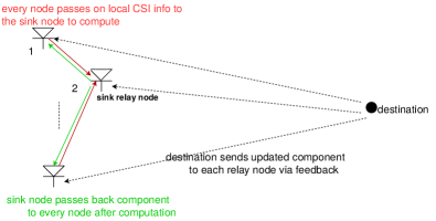
Figure 2: Distributed beamforming scheme based on CSI availability

Then the maximum achievable SINR of the system in the presence of channel errors is given by

$${\rm SINR}_{max}=P_{T}{\lambda}_{\rm largest}\{(P_{n}{\bf I}_{M}+\hat{\bf D}^{-1/2}(i)\hat{\bf U}(i)\hat{\bf D}^{-1/2}(i))^{-1}\\ \hat{\bf D}^{-1/2}(i)\hat{\bf R}_{1}(i)\hat{\bf D}^{-1/2}(i)\},$$ (43)

where the operator $\lambda_{\rm largest}\{.\}$ extracts the largest eigenvalue of the argument. The steps of the proposed LRCC-RDB technique are detailed in Table I.

TABLE I: Proposed LRCC-RDB Technique

Initialization:

${\bf w}(0)={\bf 1}$; $\hat{\bf q}(0)={\bf 1}$; ${\bf R}_{{\bf f}_{k}}(0)=0.01{\bf I}_{M}$ for $k=1,\dotsb,K$;

${\bf R}_{\bf g}(0)=0.01{\bf I}_{M}$; $\epsilon_{max}$; $N$; $P_{T}$; $\epsilon_{max}$.

For iteration $i=1,2,\dotsb$:

Compute the SCV as:

$\hat{\bf q}(i)=((i-1)\cdot\hat{\bf q}(i-1)+{\bf x}(i){z^{*}}(i))/i$

For $k=1,\dotsb,K$:

Estimate the channel covariance matrices:

${\bf R}_{{\bf f}_{k}}(i)\approx((i-1)\cdot{\bf R}_{{\bf f}_{k}}(i-1)+\hat{\bf f}_{k}(i)\hat{\bf f}_{k}^{H}(i))/i$

${\bf R}_{\bf g}(i)\approx((i-1)\cdot{\bf R}_{{\bf g}}(i-1)+\hat{\bf g}(i)\hat{\bf g}^{H}(i))/i$

Compute the error spectrum matrices for $\hat{\bf f}_{k}(i)$ and $\hat{\bf g}(i)$:

${\bf C}_{k}(i)=\epsilon_{max}{\bf R}_{{\bf f}_{k}}(i)+\frac{\epsilon_{max}^{2}}{2}||{\bf R}_{{\bf f}_{k}}(i)||_{F}{\bf I}_{M}$

${\bf C}(i)=\epsilon_{max}{\bf R}_{\bf g}(i)+\frac{\epsilon_{max}^{2}}{2}||{\bf R}_{\bf g}(i)||_{F}{\bf I}_{M}$

Compute $N$ principal eigenvectors of ${\bf C}_{k}(i)$ and ${\bf C}(i)$:

$[{\bf c}_{1,k}(i),{\bf c}_{2,k}(i),\dotsb,{\bf c}_{N,k}(i)]$ and $[{\bf c}_{1}(i),{\bf c}_{2}(i),\dotsb,{\bf c}_{N}(i)]$

Compute the projection matrix for $\hat{\bf f}_{k}(i)$ and $\hat{\bf g}(i)$:

${\bf P}_{k}(i)=[{\bf c}_{1,k}(i),{\bf c}_{2,k}(i),\dotsb,{\bf c}_{N,k}(i)]$

$[{\bf c}_{1,k}(i),{\bf c}_{2,k}(i),\dotsb,{\bf c}_{N,k}(i)]^{H}$

${\bf P}(i)=[{\bf c}_{1}(i),{\bf c}_{2}(i),\dotsb,{\bf c}_{N}(i)][{\bf c}_{1}(i),{\bf c}_{2}(i),\dotsb,{\bf c}_{N}(i)]^{H}$

Estimate $\hat{\bf f}_{k}(i)$ and $\hat{\bf g}(i)$ by subspace projections:

$\hat{\bf f}_{k}(i)=\frac{{\bf P}_{k}(i)\hat{\bf q}(i)}{{\lVert{{\bf P}_{k}(i)\hat{\bf q}(i)}\rVert}_{2}}$

$\hat{\bf g}(i)=\frac{{\bf P}(i)\hat{\bf q}(i)}{{\lVert{{\bf P}(i)\hat{\bf q}(i)}\rVert}_{2}}$

Compute $\hat{\bf R}_{k}(i)$:

$\hat{\bf R}_{k}(i)=P_{s,k}E[(\hat{\bf f}_{k}(i)\odot\hat{\bf g}(i))(\hat{\bf f}_{k}(i)\odot\hat{\bf g}(i))^{H}]$

End of $k$.

Compute quantities $\hat{\bf D}(i)$, $\hat{\bf Q}(i)$ and $\hat{\bf U}(i)$:

$\hat{\bf D}(i)={\rm diag}(\sum_{k=1}^{K}P_{s,k}[E[|\hat{f}_{1,k}(i)|^{2}],E[|\hat{f}_{2,k}(i)|^{2}],\dotsb,$

$E[\hat{f}_{M,k}(i)|^{2}]]+P_{n})$

$\hat{\bf Q}(i)=P_{n}E[\hat{\bf g}(i)\hat{\bf g}^{H}(i)]$

$\hat{\bf U}(i)=\hat{\bf Q}(i)+\sum_{k=2}^{K}\hat{\bf R}_{k}(i)$

Obtain the LRCC-RDB weight vector:

${\bf w}(i)=\sqrt{P_{T}}\hat{\bf D}^{-1/2}(i){\mathcal{P}}\{(P_{n}{\bf I}_{M}+\hat{\bf D}^{-1/2}(i)\hat{\bf U}(i)\hat{\bf D}^{-1/2}(i))^{-1}$

$\hat{\bf D}^{-1/2}(i)\hat{\bf R}_{1}(i)\hat{\bf D}^{-1/2}(i)\}$

Compute the system output SINR:

${\rm SINR}_{max}=P_{T}{\lambda}_{\rm largest}\{(P_{n}{\bf I}_{M}+\hat{\bf D}^{-1/2}(i)\hat{\bf U}(i)\hat{\bf D}^{-1/2}(i))^{-1}$

$\hat{\bf D}^{-1/2}(i)\hat{\bf R}_{1}(i)\hat{\bf D}^{-1/2}(i)\}$

End of $i$.

IV Analysis

This section presents a performance analysis of the proposed LRCC-RDB technique in terms of the MSEs for the channels and its complexity. Although the performance analysis is for distributed beamforming the main principles can also be useful for other scenarios and techniques. In the MSE analysis, we emphasize the required assumptions that the channel components ${\bf f}_{k}$, $k=1,\dotsb,K$, ${\bf g}$, the error vectors ${\bf e}_{k}$, $k=1,\dotsb,K$, ${\bf e}$ and the noise ${\bf\nu}$, $n$ are all uncorrelated with each other. We investigate the MSE performance using two different approaches, one obtains a pair of upper and lower bounds that are based on the spread of the channel covariance matrix for the channel error model adopted, which are useful to assess most RDB techniques, whereas the other approach obtains tighter bounds for subspace projection-based techniques such as the proposed LRCC-RDB technique that involves the SCV and are related to principal component analysis (PCA).

IV-A MSE Analysis

In this section, we carry out a general MSE analysis of the channel errors associated with the distributed beamforming problem. The objectives of the proposed MSE analysis are to provide an analytic investigation of the proposed LRCC-RDB and existing techniques and establish the following:

• to obtain a pair of upper and lower bounds for RDB methods that model the channel error covariance matrix as additive perturbation based on the Frobenius norm of the true channel covariance matrix and a perturbation parameter $\epsilon$ as in (24).

• to show that the proposed LRCC-RDB algorithm outperforms the RDB methods, which generally employ an additive perturbation for the channel mismatches and do not exploit prior knowledge in the form of cross-correlation and subspace structures like LRCC-RDB.

Let us first define the MSE between ${\bf f}_{k}$ and $\hat{\bf f}_{k}$ as

$$\begin{split}{\rm MSE}\{\hat{\bf f}_{k}\}_{1}&\triangleq{\rm tr}(E[(\hat{\bf f}_{k}-{\bf f}_{k})(\hat{\bf f}_{k}-{\bf f}_{k})^{H}])\\ &={\rm tr}(E[{\bf e}_{k}{\bf e}_{k}^{H}])={\rm tr}({\bf R}_{{\bf e}_{k}})\\ &={\rm tr}\Big{(}\frac{{\epsilon}_{max}}{2}||{\bf R}_{{\bf f}_{k}}||_{F}{\bf I}_{M}\Big{)}=\frac{{\epsilon}_{max}M}{2}||{\bf R}_{{\bf f}_{k}}||_{F}.\end{split}$$ (44)

Furthermore, the Frobenius norm of any positive definite matrix can be expressed as the square root of the sum of its squared eigenvalues, which results in

$$||{\bf R}_{{\bf f}_{k}}||_{F}=\sqrt{\sum_{m=1}^{M}\lambda_{m,k}^{2}},$$ (45)

where $\lambda_{m,k}$ refers to the $m$th eigenvalue of matrix ${\bf R}_{{\bf f}_{k}}$.

Let us now denote the eigenvalue spread of the matrix ${\bf R}_{{\bf f}_{k}}$ as $\sigma_{\lambda,k}$, which is defined by $|\lambda_{max,k}-\lambda_{min,k}|$, where $\lambda_{max,k}$ and $\lambda_{max,k}$ refer to the maximum eigenvalue and the minimum eigenvalue of ${\bf R}_{{\bf f}_{k}}$, respectively. Then we can obtain a lower bound for ${\rm min}\{\sum_{m=1}^{M}\lambda_{m,k}^{2}\}$ by assuming $\lambda_{1,k},\lambda_{2,k},\dotsb$, $\lambda_{m,k},\dotsb,\lambda_{M,k}$ ($\lambda_{m,k}\neq\lambda_{max,k}$) $\rightarrow 0^{+}$, which yields the following relations for the lower bound on the MSE of $\hat{\bf f}_{k}$:

$$\begin{split}{\rm min}\Big{\{}\sum_{m=1}^{M}\lambda_{m,k}^{2}\Big{\}}&>(M-1)\lambda_{min,k}^{2}+\lambda_{max,k}^{2}\\ &=(M-1)(\lambda_{max,k}-\sigma_{\lambda,k})^{2}+\lambda_{max,k}^{2}\\ &=M\lambda_{max,k}^{2}-2(M-1)\sigma_{\lambda,k}\lambda_{max,k}\\ &+(M-1)\sigma_{\lambda,k}^{2}.\end{split}$$ (46)

We can also obtain an upper bound for ${\rm max}\{\sum_{m=1}^{M}\lambda_{m,k}^{2}\}$ by assuming $\lambda_{1,k},\lambda_{2,k},\dotsb$, $\lambda_{m,k},\dotsb,\lambda_{M,k}$ ($\lambda_{m,k}\neq\lambda_{max,k}$) $\rightarrow\lambda_{max,k}^{-}$, which yields the following relations for the upper bound on the MSE of $\hat{\bf f}_{k}$:

$$\begin{split}{\rm max}\Big{\{}\sum_{m=1}^{M}\lambda_{m,k}^{2}\Big{\}}&<(M-1)\lambda_{max,k}^{2}+\lambda_{min,k}^{2}\\ &=(M-1)\lambda_{max,k}^{2}+(\lambda_{max,k}-\sigma_{\lambda,k})^{2}\\ &=M\lambda_{max,k}^{2}-2\sigma_{\lambda,k}\lambda_{max,k}+\sigma_{\lambda,k}^{2}.\end{split}$$ (47)

By substituting (45) into (46) and (47), we obtain

$${\rm min}\{||{\bf R}_{{\bf f}_{k}}||_{F}\}>\\ \sqrt{M\lambda_{max,k}^{2}-2(M-1)\sigma_{\lambda,k}\lambda_{max,k}+(M-1)\sigma_{\lambda,k}^{2}},$$ (48)

$${\rm max}\{||{\bf R}_{{\bf f}_{k}}||_{F}\}<\sqrt{M\lambda_{max,k}^{2}-2\sigma_{\lambda,k}\lambda_{max,k}+\sigma_{\lambda,k}^{2}}.$$ (49)

Since we have ${\rm min}\{||{\bf R}_{{\bf f}_{k}}||_{F}\}\leq||{\bf R}_{{\bf f}_{k}}||_{F}\leq{\rm max}\{||{\bf R}_{{\bf f}_{k}}||_{F}\},$ then we can obtain the upper and lower bounds for $||{\bf R}_{{\bf f}_{k}}||_{F}$ by substituting the relations in (46) and (47) in (48) and (49), respectively, resulting in

$$\sqrt{M\lambda_{max,k}^{2}-2(M-1)\sigma_{\lambda,k}\lambda_{max,k}+(M-1)\sigma_{\lambda,k}^{2}}\\ <||{\bf R}_{{\bf f}_{k}}||_{F}<\\ \sqrt{M\lambda_{max,k}^{2}-2\sigma_{\lambda,k}\lambda_{max,k}+\sigma_{\lambda,k}^{2}},$$ (50)

which is then substituted in (44) and yields the bounds for the MSE:

$$\frac{{\epsilon}_{max}M}{2}\sqrt{M\lambda_{max,k}^{2}-2(M-1)\sigma_{\lambda,k}\lambda_{max,k}+(M-1)\sigma_{\lambda,k}^{2}}\\ <{\rm MSE}\{\hat{\bf f}_{k}\}_{1}<\\ \frac{{\epsilon}_{max}M}{2}\sqrt{M\lambda_{max,k}^{2}-2\sigma_{\lambda,k}\lambda_{max,k}+\sigma_{\lambda,k}^{2}}.$$ (51)

The bounds described in (51) give an insight on how the MSE of the $k$th component of $\hat{\bf F}$ is bounded by the maximum (principal) eigenvalue $\lambda_{max,k}$ of the channel covariance matrix ${\bf R}_{{\bf f}_{k}}$ and the eigenvalue spread $\sigma_{\lambda,k}$ of its Frobenius norm $||{\bf R}_{{\bf f}_{k}}||_{F}$. The same procedure can be carried out for analyzing the MSE of channel $\hat{\bf g}$, which is not presented here to avoid a repetitive development. We can employ both lower bounds of the channel components $\hat{\bf f}_{k}$ and channel $\hat{\bf g}$ as their minimum MSEs (MMSEs) to compute the MMSEs of $\hat{\bf F}$ and $\hat{\bf g}$ as

$${\rm MMSE}\{\hat{\bf F}\}=\sum_{k=1}^{K}{\rm MMSE}\{\hat{\bf f}_{k}\}=\frac{{\epsilon}_{max}M}{2}\\ \sum_{k=1}^{K}\sqrt{M\lambda_{max,k}^{2}-2(M-1)\sigma_{\lambda,k}\lambda_{max,k}+(M-1)\sigma_{\lambda,k}^{2}},$$ (52)

$$\begin{split}&{\rm MMSE}\{\hat{\bf g}\}=\frac{{\epsilon}_{max}M}{2}\\ &\sqrt{M\lambda_{max}^{2}-2(M-1)\sigma_{\lambda}\lambda_{max}+(M-1)\sigma_{\lambda}^{2}},\end{split}$$ (53)

respectively. Note that $\lambda_{max}$ here is a scalar representing the largest eigenvalue of ${\bf R}_{\bf g}$ and $\sigma_{\lambda}$ is the corresponding eigenvalue spread. As an example, we set the total number of relays and signal sources $M=8$, $\epsilon_{max}=0.2$ and the input SNR is set to $10$dB. Then we test two cases with $\sigma_{\lambda,k}=0.9\lambda_{max,k}$ and $\sigma_{\lambda,k}=0.5\lambda_{max,k}$ and illustrate the variations of those bounds in Figs. 3 and 4, respectively. Because we use linear relations between $\sigma_{\lambda,k}$ and $\lambda_{max,k}$, proportional relations between the MSE bounds and $\lambda_{max,k}$ are reflected as can be seen in Figs. 3 and 4. In addition, we generate the signals that are processed by the sensor array and compute the actual MSE values of the mismatched channels which are independent of the RDB algorithms, according to the above conditions and compare the results to the analytic bounds in Figs. 3 and 4. The results are obtained by taking the average MSE result from $k=1,\dotsb,K$. The sets of matrix eigenvalues are selected to be as close as possible to the analytic conditions assumed for the sake of comparison. Also, by comparing the values and variations of the MSE bounds in Figs. 3 and 4, we can see that there is no obvious difference between the upper bounds. However, with a smaller eigenvalue spread $\sigma_{\lambda,k}$, the lower bound gets closer to the upper bound. The results obtained by generating the signals processed by the sensor array indicate that with a small $\lambda_{max,k}$ the MSE gets closer to the upper bound.

Figure 3: MSE bounds versus $\lambda_{max,k}$, $\sigma_{\lambda,k}=0.9\lambda_{max,k}$

Figure 4: MSE bounds versus $\lambda_{max,k}$, $\sigma_{\lambda,k}=0.5\lambda_{max,k}$

IV-B Analysis of Low-rank and Cross-Correlation Processing

In this section, we present the performance analysis of the proposed LRCC-RDB technique. In particular, this analysis is specific to the low-rank and cross-correlation processing performed by the proposed LRCC-RDB method. At first we aim to exploit the properties of the cross-correlation vector ${\bf q}(i)$ estimated in (21). For convenience, we omit the time index $i$ in the following analysis. By definition, we have

$$\begin{split}{\bf q}\triangleq E[z^{*}{\bf x}]&=E[(\hat{\bf g}^{T}{\bf W}{\bf x}+n)^{*}{\bf x}]\\ &=E[(\hat{\bf g}^{H}{\bf W}^{*}{\bf x}^{*}+n^{*})(\hat{\bf F}{\bf s}+{\bf\nu})].\end{split}$$ (54)

Since ${\bf W}$ is diagonal, we have ${\bf W}^{*}={\bf W}^{H}$. By assuming that the noise $n$ is uncorrelated with ${\bf s}$ and ${\bf\nu}$, the terms $E[n^{*}\hat{\bf F}{\bf s}]$ and $E[n^{*}{\bf\nu}]$ are equal to zero and can be discarded. Then from (54) we have

$$\begin{split}{\bf q}&=E[\hat{\bf g}^{H}{\bf W}^{*}{\bf x}^{*}\hat{\bf F}{\bf s}+\hat{\bf g}^{H}{\bf W}^{*}{\bf x}^{*}{\bf\nu}]\\ &=E[\hat{\bf g}^{H}{\bf W}^{*}(\hat{\bf F}^{*}{\bf s}^{*}+{\bf\nu}^{*})\hat{\bf F}{\bf s}+\hat{\bf g}^{H}{\bf W}^{*}{\bf x}^{*}{\bf\nu}]\\ &=E[\hat{\bf F}{\bf s}{\bf s}^{H}\hat{\bf F}^{H}{\bf W}\hat{\bf g}]+E[{\bf\nu}{\bf\nu}^{H}{\bf W}\hat{\bf g}],\end{split}$$ (55)

where $\hat{\bf F}=[\hat{\bf f}_{1},\dotsb,\hat{\bf f}_{K}]$ is the mismatched channel matrix and ${\bf s}=[s_{1},\dotsb,s_{K}]^{T}$. Now we expand the expressions for both $\hat{\bf F}$ and ${\bf s}$ in (55) while assuming that the source signals are uncorrelated with each other. Then we obtain

$$\begin{split}{\bf q}&=E[(\sum_{k=1}^{K}\hat{\bf f}_{k}{s}_{k})(\sum_{k=1}^{K}\hat{\bf f}_{k}{s}_{k})^{H}{\bf W}\hat{\bf g}]+E[{\bf\nu}{\bf\nu}^{H}{\bf W}\hat{\bf g}]\\ &=E[\sum_{k=1}^{K}{s}_{k}{s}_{k}^{*}\hat{\bf f}_{k}\hat{\bf f}_{k}^{H}{\bf W}\hat{\bf g}]+E[{\bf\nu}{\bf\nu}^{H}{\bf W}\hat{\bf g}].\end{split}$$ (56)

At this stage, we emphasize that the analysis procedure for channel $\hat{\bf f}_{k}$ is independent from $\hat{\bf g}$ as we will project the same cross-correlation vector onto their subspace independently even though the procedures are the same. For ease of exposition and comparison with the MSE analysis of the previous subsection, we focus on the analysis for ${\bf f}_{k}$ only and employ ${\bf\xi}=E[{\bf W}\hat{\bf g}]$. Therefore, if we substitute $\hat{\bf f}_{k}={\bf f}_{k}+{\bf e}_{k}$ in (56) and replace $E[{s}_{k}{s}_{k}^{*}]$ and $E[{\bf\nu}{\bf\nu}^{H}]$ with $P_{s,k}$ and $P_{n}$, respectively, (56) can be simplified to

$$\begin{split}{\bf q}&=E[\sum_{k=1}^{K}P_{s,k}{\bf f}_{k}{\bf f}_{k}^{H}+{\bf e}_{k}{\bf e}_{k}^{H}]{\bf\xi}+P_{n}{\bf\xi}\\ &=(\sum_{k=1}^{K}P_{s,k}E[({\bf R}_{{\bf f}_{k}}+{\bf R}_{{\bf e}_{k}})]+P_{n}){\bf\xi}.\end{split}$$ (57)

Let us now define the $k$th cross-correlation vector component as

$${\bf q}_{k}\triangleq(P_{s,k}E[({\bf R}_{{\bf f}_{k}}+{\bf R}_{{\bf e}_{k}})]){\bf\xi},$$ (58)

and write the cross-correlation vector as

$${\bf q}\triangleq\sum_{k=1}^{K}{\bf q}_{k}+P_{n}{\bf\xi}.$$ (59)

LRCC-RBD applies a subspace projection to the cross-correlation vector by substituting (59) in $\hat{\bf f}_{k}={\bf P}_{k}{\bf q}$ (assuming it is normalized as in (32)), which results in

$$\hat{\bf f}_{k}={\bf P}_{k}(\sum_{k=1}^{K}{\bf q}_{k}+P_{n}{\bf\xi}).$$ (60)

If we assume that by projecting any cross-correlation vector component ${\bf q}_{l}$ generated from the channel components $\hat{\bf f}_{l}$ ($1\leq l(l\neq k)\leq K$) onto the subspace projection matrix ${\bf P}_{k}$ we have ${\bf P}_{k}{\bf q}_{l}=0$, then (60) can be simplified to

$$\hat{\bf f}_{k}={\bf P}_{k}({\bf q}_{k}+P_{n}{\bf\xi})={\bf P}_{k}(P_{s,k}E[({\bf R}_{{\bf f}_{k}}+{\bf R}_{{\bf e}_{k}})]+P_{n}){\bf\xi}.$$ (61)

From the MSE definition in (44), we have

$${\rm MSE}\{\hat{\bf f}_{k}\}_{2}={\rm tr}(E[(\hat{\bf f}_{k}-{\bf f}_{k})(\hat{\bf f}_{k}-{\bf f}_{k})^{H}])=E[(\hat{\bf f}_{k}-{\bf f}_{k})^{H}(\hat{\bf f}_{k}-{\bf f}_{k})].$$

After substituting (61) in (44), we obtain

$$\begin{split}{\rm MSE}\{\hat{\bf f}_{k}\}_{2}&=E[({\bf P}_{k}(P_{s,k}E[({\bf R}_{{\bf f}_{k}}+{\bf R}_{{\bf e}_{k}})]+P_{n}){\bf\xi}-{\bf f}_{k})^{H}\\ &\quad({\bf P}_{k}(P_{s,k}E[({\bf R}_{{\bf f}_{k}}+{\bf R}_{{\bf e}_{k}})]+P_{n}){\bf\xi}-{\bf f}_{k})].\end{split}$$ (62)

After expanding (62), we get

$$\begin{split}{\rm MSE}\{\hat{\bf f}_{k}\}_{2}&=E[{\bf\xi}^{H}(P_{s,k}{\bf R}_{{\bf f}_{k}}+P_{s,k}{\bf R}_{{\bf e}_{k}}+P_{n}){\bf P}_{k}^{H}{\bf P}_{k}(P_{s,k}\\ &\quad{\bf R}_{{\bf f}_{k}}+P_{s,k}{\bf R}_{{\bf e}_{k}}+P_{n}){\bf\xi}]-2E[{\bf f}_{k}^{H}{\bf P}_{k}(P_{s,k}{\bf R}_{{\bf f}_{k}}\\ &\quad+P_{s,k}{\bf R}_{{\bf e}_{k}}+P_{n}){\bf\xi}]+E[{\bf f}_{k}^{H}{\bf f}_{k}].\end{split}$$ (63)

It should be noticed that ${\bf P}_{k}^{H}{\bf P}_{k}={\bf P}_{k}={\bf P}_{k}^{H}$ as the projection of a subspace projection matrix onto itself results in the same projection matrix. In addition, we have ${\bf f}_{k}^{H}{\bf P}_{k}={\bf f}_{k}^{H}$ in the second term of (63), which can be verified as follows. Since we have ${\bf f}_{k}=E[{\bf P}_{k}{\bf q}_{k}]$ by pre-multiplying both sides by ${\bf P}_{k}^{H}$ then we have ${\bf P}_{k}^{H}{\bf f}_{k}=E[{\bf P}_{k}^{H}{\bf P}_{k}{\bf q}_{k}]=E[{\bf P}_{k}{\bf q}_{k}]={\bf f}_{k}$. Then by taking the Hermitian transpose on both sides gives ${\bf f}_{k}^{H}{\bf P}_{k}={\bf f}_{k}^{H}$. Therefore, (63) can be rewritten as

$$\begin{split}{\rm MSE}\{\hat{\bf f}_{k}\}_{2}&=E[{\bf\xi}^{H}(P_{s,k}{\bf R}_{{\bf f}_{k}}+P_{s,k}{\bf R}_{{\bf e}_{k}}+P_{n}){\bf P}_{k}(P_{s,k}{\bf R}_{{\bf f}_{k}}\\ &\quad+P_{s,k}{\bf R}_{{\bf e}_{k}}+P_{n}){\bf\xi}]-2E[{\bf f}_{k}^{H}(P_{s,k}{\bf R}_{{\bf f}_{k}}+P_{s,k}{\bf R}_{{\bf e}_{k}}\\ &\quad+P_{n}){\bf\xi}]+E[{\bf f}_{k}^{H}{\bf f}_{k}].\end{split}$$ (64)

After expanding the terms with the multiplications, eliminating the uncorrelated ones and taking into account that ${\bf f}_{k}$ is normalized, i.e., $E[{\bf f}_{k}^{H}{\bf f}_{k}]=1$, we obtain

$$\begin{split}{\rm MSE}\{\hat{\bf f}_{k}\}_{2}&=E[{\bf\xi}^{H}(P^{2}_{s,k}{\bf R}_{{\bf e}_{k}}{\bf P}_{k}{\bf R}_{{\bf e}_{k}}+P_{n}P_{s,k}{\bf P}_{k}{\bf R}_{{\bf e}_{k}}\\ &\quad+P_{n}^{2}{\bf P}_{k}){\bf\xi}+1].\end{split}$$ (65)

By substituting (24) in (65) and performing further simplifications, we get

$$\begin{split}{\rm MSE}\{\hat{\bf f}_{k}\}_{2}&=E[(P^{2}_{s,k}\epsilon^{2}||{\bf R}_{{\bf f}_{k}}||^{2}_{F}+P_{n}P_{s,k}\epsilon||{\bf R}_{{\bf f}_{k}}||_{F}+P_{n}^{2})\\ &\quad{\bf\xi}^{H}{\bf P}_{k}{\bf\xi}+{\bf f}_{k}^{H}{\bf f}_{k}]\\ &=(\frac{1}{3}P^{2}_{s,k}\epsilon^{2}_{max}E[||{\bf R}_{{\bf f}_{k}}||_{F}]^{2}+\frac{1}{2}P_{n}P_{s,k}\epsilon_{max}E[||{\bf R}_{{\bf f}_{k}}||_{F}]\\ &\quad+P_{n}^{2}){\bf\xi}^{H}E[{\bf P}_{k}]{\bf\xi}+1,\end{split}$$ (66)

which monotonically increases with respect to $E[||{\bf R}_{{\bf f}_{k}}||_{F}]$. However, the results of the analysis can become more insightful if we compare the MSE obtained in the two approaches considered in this section. Let us denote them as ${\rm MSE}\{\hat{\bf f}_{k}\}_{1}$ (described in (44)) and ${\rm MSE}\{\hat{\bf f}_{k}\}_{2}$ (described in (66)), respectively, and ${\bf\xi}^{H}E[{\bf P}_{k}]{\bf\xi}$ as $\tau$. If we compute their difference we have

$$\begin{split}{\rm MSE}\{\hat{\bf f}_{k}\}_{2}-{\rm MSE}\{\hat{\bf f}_{k}\}_{1}&=\bigg{(}\frac{1}{3}P^{2}_{s,k}\epsilon^{2}_{max}E[||{\bf R}_{{\bf f}_{k}}||_{F}]^{2}\\ &\quad+\frac{1}{2}P_{n}P_{s,k}\epsilon_{max}E[||{\bf R}_{{\bf f}_{k}}||_{F}]+P_{n}^{2}\bigg{)}\tau\\ &\quad+1-\frac{M}{2}\epsilon_{max}E[||{\bf R}_{{\bf f}_{k}}||_{F}].\end{split}$$ (67)

If we take the partial derivative of (67) with respect to $\tau$, then we have

$$\frac{\partial\{{\rm MSE}\{\hat{\bf f}_{k}\}_{2}-{\rm MSE}\{\hat{\bf f}_{k}\}_{1}\}}{\partial{\tau}}>0,$$ (68)

which implies that ${\rm MSE}\{\hat{\bf f}_{k}\}$ is proportionally and monotonically increasing with respect to $\tau$. From (49) we have

$${\rm max}\{||{\bf R}_{{\bf f}_{k}}||_{F}\}<\sqrt{M\lambda_{max,k}^{2}-2\sigma_{\lambda,k}\lambda_{max,k}+\sigma_{\lambda,k}^{2}}<\sqrt{M}\lambda_{max,k},$$

which yields

$$\begin{split}{\rm MSE}\{\hat{\bf f}_{k}\}_{2}-{\rm MSE}\{\hat{\bf f}_{k}\}_{1}&<\bigg{(}\frac{1}{3}P^{2}_{s,k}\epsilon^{2}_{max}M\lambda_{max,k}^{2}\\ &\quad+\frac{1}{2}P_{n}P_{s,k}\epsilon_{max}\sqrt{M}\lambda_{max,k}+P_{n}^{2}\bigg{)}\tau\\ &\quad+1-\frac{M}{2}\epsilon_{max}\sqrt{M}\lambda_{max,k}.\end{split}$$ (69)

In other words, if the right-hand side of (69) is less than $0$ when $\tau$ satisfies

$$\tau<\frac{\frac{M}{2}\epsilon_{max}\sqrt{M}\lambda_{max,k}-1}{\frac{1}{3}P^{2}_{s,k}\epsilon^{2}_{max}M\lambda_{max,k}^{2}+\frac{1}{2}P_{n}P_{s,k}\epsilon_{max}\sqrt{M}\lambda_{max,k}+P_{n}^{2}},$$ (70)

and

$${\rm MSE}\{\hat{\bf f}_{k}\}_{2}-{\rm MSE}\{\hat{\bf f}_{k}\}_{1}<0$$

is true for all possible values of $E[||{\bf R}_{{\bf f}_{k}}||_{F}]$, which indicates a smaller MSE result from approach 2 (${\rm MSE}\{\hat{\bf f}_{k}\}_{2}$) as compared to approach 1 (${\rm MSE}\{\hat{\bf f}_{k}\}_{1}$). Interestingly, this indicates that using prior knowledge about the mismatch in the form of low-rank subspace and cross-correlation processing can result in smaller values of MSE. However, the only term of $\tau$ that has to be determined is the subspace projection matrix ${\bf P}_{k}$, which is dependent on its subspace properties and can be further exploited by eigenvalue interpolation methods [72].

Based on [73] and assuming that the channels and input data have Gaussian distribution, the MMSE and SINR of the system are related by

$${\rm MMSE}\{z\}=\frac{1}{1+{\rm SINR}_{max}},$$ (71)

where the ${\rm SINR}_{max}$ is obtained in (43). For simplicity, let us drop the time index $i$ and denote the term $(P_{n}{\bf I}_{M}+\hat{\bf D}^{-1/2}\hat{\bf U}\hat{\bf D}^{-1/2})^{-1}\hat{\bf D}^{-1/2}\hat{\bf R}_{1}\hat{\bf D}^{-1/2}$ in (43) and (42) as

$${\bf\Theta}=(P_{n}{\bf I}_{M}+\hat{\bf D}^{-1/2}\hat{\bf U}\hat{\bf D}^{-1/2})^{-1}\hat{\bf D}^{-1/2}\hat{\bf R}_{1}\hat{\bf D}^{-1/2}.$$ (72)

According to the properties of eigenvalues and eigenvectors, we know that

$${\bf\Theta}{\mathcal{P}}\{\bf\Theta\}=\lambda_{largest}\{\bf\Theta\}{\mathcal{P}}\{\bf\Theta\}.$$ (73)

If we pre-multiply both sides of (42) by $\hat{\bf D}^{1/2}$ and drop the time index, it becomes

$$\frac{\hat{\bf D}^{1/2}{\bf w}}{\sqrt{P}_{T}}={\mathcal{P}}\{\bf\Theta\}.$$ (74)

Then, by substituting (74) in (73), we obtain

$${\bf\Theta}\hat{\bf D}^{1/2}{\bf w}=\lambda_{largest}\{\bf\Theta\}\hat{\bf D}^{1/2}{\bf w},$$ (75)

which through the use of the weight vector norm constraint ${\bf w}^{H}{\bf w}=1$ gives the expression for $\lambda_{largest}\{\bf\Theta\}$:

$$\lambda_{largest}\{\bf\Theta\}={\bf w}^{H}\hat{\bf D}^{-1/2}{\bf\Theta}\hat{\bf D}^{1/2}{\bf w}.$$ (76)

Finally, by substituting (76) in (43), ${\rm SINR}_{max}$ is rewritten as

$${\rm SINR}_{max}=P_{T}\lambda_{largest}\{\bf\Theta\}=P_{T}{\bf w}^{H}\hat{\bf D}^{-1/2}{\bf\Theta}\hat{\bf D}^{1/2}{\bf w}$$ (77)

while the MMSE of $z$ is computed from (71) as

$${\rm MMSE}\{z\}=\frac{1}{1+P_{T}{\bf w}^{H}\hat{\bf D}^{-1/2}{\bf\Theta}\hat{\bf D}^{1/2}{\bf w}},$$ (78)

In (78), ${\rm MMSE}\{z\}$ is determined by ${\bf w}$ and ${\bf\Theta}$, which are both directly obtained from (42) and (72) and are only dependent on the variables of the channel estimates $\hat{\bf f}_{k}$, $k=1,\dotsb,K$ and ${\bf g}$. We remark that the weight vector ${\bf w}$ (or its diagonal matrix form ${\bf W}$) is estimated and expressed using $\hat{\bf f}_{k}$, $k=1,\dotsb,K$ and ${\bf g}$, as we know that $\hat{\bf D}$, $\hat{\bf R}_{1}$, $\hat{\bf U}$ are all based on $\hat{\bf f}_{k}$, $k=1,\dotsb,K$ and ${\bf g}$, where the MMSE of ${\bf g}$ can be obtained in a similar way as $\hat{\bf f}_{k}$ and hence the derivation is omitted. Therefore, the MMSE of $z$ for the proposed LRCC-RDB technique only depends on the MMSE estimates for $\hat{\bf f}_{k}$ and $\hat{\bf g}$. In this case, ${\rm MMSE}\{z\}$ is proportional to ${\rm MMSE}\{\hat{\bf f}_{k}\}$ and ${\rm MMSE}\{\hat{\bf g}\}$, i.e., ${\rm MMSE}\{z\}\propto{\rm MMSE}\{\hat{\bf f}_{k}\},{\rm MMSE}\{\hat{\bf g}\}$. Since we have proved that under certain assumptions the estimate $\hat{\bf f}_{k}$ obtained by the proposed LRCC-RDB approach is better than those of other analyzed techniques then the same analysis procedure applies to $\hat{\bf g}$. Therefore, RDB techniques which adopt the LRCC-RDB technique are able to achieve smaller ${\rm MMSE}\{\hat{\bf f}_{k}\}$ and ${\rm MMSE}\{\hat{\bf g}\}$, and consequently a smaller ${\rm MMSE}\{z\}$ than those of other RDB methods, as verified in the simulation results.

IV-C Complexity Analysis

This subsection presents an analysis of the computational complexity of LRCC-RDB and comparisons with existing robust approaches such as the most common worst-case approaches, which are typically solved using an interior point method (e.g. [17, 19, 20, 74]) and the probabilistic based stochastic approach introduced in [16], all of which are shown in Table II. It should be noted that we compare the computational complexities of the approaches regardless of their system design objectives, which could target the minimization of the total relay transmit power with a QoS (output SNR or SINR) constraint (e.g. [17, 19, 20]). A limited number of techniques like the approach reported in [74] aims to maximize the QoS with individual relay transmit power, whereas LRCC-RDB aims to maximize the output SINR with a total relay transmit power constraint and does not require any online optimization procedure. Due to the highly involved procedures and recursions of online convex optimization employed by the existing algorithms, we only compare the polynomial bound of each of them. Note that LRCC-RDB only incurs cubic complexity (${\mathcal{O}}(M^{3})$) when computing the weight vector. Specifically, $\hat{\bf D}^{-1/2}(i)$ is a diagonal matrix, which means the computations of $\hat{\bf D}^{-1/2}(i)\hat{\bf U}(i)\hat{\bf D}^{-1/2}(i)$ and $\hat{\bf D}^{-1/2}(i)\hat{\bf R}_{1}(i)\hat{\bf D}^{-1/2}(i)$ are both at a cost of ${\mathcal{O}}(M^{2})$. The only costly operations are: the matrix inversion $(P_{n}{\bf I}_{M}+\hat{\bf D}^{-1/2}(i)\hat{\bf U}(i)\hat{\bf D}^{-1/2}(i))^{-1}$, the matrix multiplication between $(P_{n}{\bf I}_{M}+\hat{\bf D}^{-1/2}(i)\hat{\bf U}(i)\hat{\bf D}^{-1/2}(i))^{-1})$ and $(\hat{\bf D}^{-1/2}(i)\hat{\bf R}_{1}(i)\hat{\bf D}^{-1/2}(i))$, the eigen decomposition of the resulting matrix after multiplication. Each of these three operations requires a complexity of ${\mathcal{O}}(M^{3})$ and only needs to be computed once. As previously explained, we only need to compute the above required operations once for a data block when the channel is within the same coherence time, that is, only one matrix inversion, one matrix multiplication and one eigen decomposition are required for a data block. For SOCP and SDP, there are multiple iterations within the solver per snapshot as well. The key point is that either per snapshot or when computing the weights once in a data block, the proposed approach is computationally simpler and provides improved resilience and robustness.

TABLE II: Computational Complexity

RDB algorithms	Flops per snapshot
Worst-case with SDP [17, 19]	${\mathcal{O}}(M^{6.5})$
Worst-case with SOCP [20, 74]	${\mathcal{O}}(M^{3.5})$
Stochastic approach with SDP [16]	${\mathcal{O}}(M^{9.5})$
Proposed LRCC-RDB method	${\mathcal{O}}(M^{3})$

V Simulations

In this section we conduct simulations to assess the proposed LRCC-RDB method for several scenarios, namely, the case of perfect CSI, the case in which no robust method is used and the CSI is imperfect, and the cases in which CSI is imperfect and several existing robust approaches [11, 15, 17, 18, 19, 20, 21, 23, 24, 74] (i.e. worst-case SDP online programming) are used. The figures of metric considered include the system output SINR versus input SNR as well as the maximum allowable total transmit power $P_{T}$. We also examine incoherent scenarios, where some of the interferers are strong enough as compared to the desired signal and the noise. In all simulations, the system input SNR is known and can be controlled by adjusting only the noise power. Both channels $\hat{\bf F}$ and $\hat{\bf g}$ are modeled by the Rayleigh distribution. The shadowing and path loss effects are taken into account with the path loss exponent set to $\rho=2$, the source-to-destination power path loss set to $L=10$dB and the shadowing spread set to $\sigma_{s}=3$dB. As discussed in Section II, the relative source-to-relay link distances $d_{s,r_{m}}$ are selected from a set of uniform random variables distributed between $0.5$ to $0.9$, with corresponding relay-source-destination angles $\theta_{r_{m},s,d}$ randomly chosen from an angular range between $-\pi/2$ and $\pi/2$. The total number of relays and signal sources are set to $M=8$ and $K=3$, respectively, and we set $\sigma_{b_{k}}=1$ for $k=1,\dotsb,K$. The interference-to-noise ratio (INR) of the system is fixed at $10$dB unless otherwise specified. A total number of $100$ snapshots are considered. The number of principal components is selected according to the criterion mentioned in Section III to optimize the performance of LRCC-RDB, as illustrated in Fig. 5. Assigning any value larger than the minimum sufficient value of $N$ leads to insignificant performance improvements and extra complexity.

Figure 5: Principal components selection

In the first example, we examine the SINR performance against different values of the mismatch parameter $\epsilon_{max}$ ($0.1\leq\epsilon_{max}\leq 1$) in Fig. 6, while limiting the maximum allowable transmit power to $P_{T}=1$dBW and fixing the input SNR at $10$dB for all the compared cases. The powers of the interferers are equally distributed across the interferers. The worst-case SDP method is adopted from [17], in which the values of $\epsilon_{max}$ are set to be consistent with all the mismatched matrix quantities. The results show that the proposed LRCC-RDB method preserves the robustness against the increase of the level of channel errors and remains close to the case of perfect CSI, whereas the worst-case SDP method suffers performance degradation against the increase of the level of channel errors.

Figure 6: SINR versus $\epsilon_{max}$, $P_{T}=1$dBW, SNR=$10$dB, INR=$10$dB

In the second example, we examine the SINR performance versus the variation of maximum allowable total transmit power $P_{T}$ (i.e. $1$dBW to $5$dBW) by fixing the input SNR at $10$dB. We consider the same INR and that all interferers have the same power. In this example, we set the perturbation parameter to $\epsilon_{max}=0.5$ for all compared techniques. In Fig. 7, it shows the output SINR increases as we increase the limit for the maximum allowable transmit power and this results in a substantial difference when a robust approach is used. LRCC-RDB outperforms the worst-case SDP algorithm and performs close to the case with perfect CSI.

Figure 7: SINR versus $P_{T}$, SNR=$10$dB, $\epsilon_{max}=0.5$, INR=$10$dB

In the last example, we increase the system INR from $10$dB to $20$dB. We consider $K=3$ users (which means there are two interferers in total) but rearrange the powers of the interferers so that one of them is much stronger than the other. Specifically, we examine the compared approaches in an incoherent scenario and set the power ratio of the stronger interferer over the weaker one to $10$. The maximum allowable total transmit power $P_{T}$ and the perturbation parameter $\epsilon_{max}$ are set to $1$dBW and $0.2$, respectively. We observe the SINR performance versus SNR for these techniques and illustrate the results in Fig. 8. Then we set the system SNR to $10$dB and observe the output SINR performance versus snapshots as in Fig. 9. It can be seen that all the approaches have performance degradations due to the strong interferers as well as their power distribution. However, LRCC-RDB shows robustness in terms of output SINR performance against the presence of strong interferers with unbalanced power distribution. In particular, with relative high system SNRs, LRCC-RDB is able to perform extremely close to the case of perfect CSI.

Figure 8: SINR versus SNR, $P_{T}=1$dBW, $\epsilon_{max}=0.2$, INR=$20$dB

Figure 9: SINR versus snapshots, $P_{T}=1$dBW, $\epsilon_{max}=0.2$, SNR=$10$dB, INR=$20$dB

VI Conclusion

We have devised a novel RDB approach based on the exploitation of the cross-correlation between the received data from the relays and the system output, as well as a low-rank subspace projection method to estimate the channel errors. In the proposed LRCC-RDB method, a total relay transmit power constraint has been considered and the objective is to maximize the output SINR. A performance analysis of LRCC-RDB has been carried out and shown that it outperforms approaches that do not exploit prior knowledge about the mismatch. LRCC-RDB does not require any costly online optimization procedure and the simulation results have shown excellent performance as compared to existing approaches and can be applied to detection and estimation in wireless communications [75, 76, 77, 78, 79, 80, 81, 34, 82, 83, 84, 85, 86, 87, 88, 89, 90, 91, 92, 93, 94].

References

- [1] R. Mudumbai, D. B. III, U. Madhow, and H. Poor, “Distributed transmit beamforming challenges and recent progress,” IEEE Communications Magazine, vol. 47, no. 4, pp. 102–110, 2009.
- [2] A. B. Gershman, N. D. Sidiropoulos, S. Shahbazpanahi, M. Bengtsson, and B. Ottersten, “Convex optimization-based beamforming,” IEEE Signal Processing Magazine, vol. 27, no. 3, pp. 62–75, May 2010.
- [3] J. Uher, T. A. Wysocki, and B. J. Wysocki, “Review of distributed beamforming,” Journal of Telecommunications and Information Technology, 2011.
- [4] V. H. Nassab, S. Shahbazpanahi, A. Grami, and Z. Luo, “Distributed beamforming for relay networks based on second-order statistics of the channel state information,” IEEE Trans. Signal Process., vol. 56, no. 9, pp. 4306–4316, Sep 2008.
- [5] K. Zarifi, S. Zaidi, S. Affes, and A. Ghrayeb, “A distributed amplify-and-forward beamforming technique in wireless sensor networks,” IEEE Trans. Signal Process., vol. 59, no. 8, pp. 3657–3674, Aug 2011.
- [6] H. Ruan and R. C. de Lamare, “Joint mmse consensus and relay selection algorithms for distributed beamforming,” in 2016 IEEE Sensor Array and Multichannel Signal Processing Workshop (SAM), July 2016.
- [7] ——, “Joint msinr and relay selection algorithms for distributed beamforming,” in 2016 IEEE Sensor Array and Multichannel Signal Processing Workshop (SAM), July 2016.
- [8] Y. Jing and H. Jafarkhani, “Network beamforming using relays with perfect channel information,” IEEE Trans. Information Theory, vol. 55, no. 6, pp. 2499–2517, June 2009.
- [9] V. Havary-Nassab, S. Shahbazpanahi, and A. Grami, “Optimal distributed beamforming for two-way relay networks,” IEEE Trans. Signal Process., vol. 58, no. 3, pp. 1238–1250, March 2010.
- [10] Y. Cao and C. Tellambura, “Joint distributed beamforming and power allocation in underlay cognitive two-way relay links,” IEEE Trans. Signal Process., vol. 62, no. 22, pp. 5950–5961, Sep 2014.
- [11] L. Zhang, W. Liu, A. Quddus, M. Dianati, and R. Tafazolli, “Adaptive distributed beamforming for relay networks based on local channel state information,” IEEE Trans. on Signal and Information Process. over Networks, vol. 1, no. 2, pp. 117–128, June 2015.
- [12] J. Zhu, R. S. Blum, X. Lin, and Y. Gu, “Robust transmit beamforming for parameter estimation using distributed sensors,” IEEE Communications Letters, vol. 20, no. 7, pp. 1329–1332, July 2016.
- [13] J. Ma and W. Liu, “Robust iterative transceiver beamforming for multipair two-way distributed relay networks,” IEEE Access, vol. 5, pp. 24 656–24 667, 2017.
- [14] A. I. Koutrouvelis, T. W. Sherson, R. Heusdens, and R. C. Hendriks, “A low-cost robust distributed linearly constrained beamformer for wireless acoustic sensor networks with arbitrary topology,” IEEE/ACM Transactions on Audio, Speech, and Language Processing, vol. 26, no. 8, pp. 1434–1448, Aug 2018.
- [15] D. Ponukumati, F. Gao, and C. Xing, “Robust peer-to-peer relay beamforming a probabilistic approach,” IEEE Communications Letters, vol. 17, no. 2, pp. 305–308, Jan 2013.
- [16] M. A. Maleki, S. Mehrizi, and M. Ahmadian, “Distributed robust beamforming in multi-user relay network,” in IEEE Wireless Communications and Networking Conference (WCNC), 2014, pp. 904–907.
- [17] B. Mahboobi, M. Ardebilipour, A. Kalantari, and E. Soleimani-Nasab, “Robust cooperative relay beamforming,” IEEE Wireless Communications Letters, vol. 2, no. 4, pp. 399–402, May 2013.
- [18] P. Hsieh, Y. Lin, and S. Chen, “Robust distributed beamforming design in amplify-and-forward relay systems with multiple user pairs,” in 23rd International Conference on Software, Telecommunications and Computer Networks (SoftCOM), Sep 2015, pp. 371–375.
- [19] P. Ubaidulla and A. Chockalingam, “Robust distributed beamforming for wireless relay networks,” in IEEE 20th International Symposium on Personal, Indoor and Mobile Radio Communications, Sep 2009, pp. 2345–2349.
- [20] S. Salari, M. Z. Amirani, I. Kim, D. Kim, and J. Yang, “Distributed beamforming in two-way relay networks with interference and imperfect csi,” IEEE Trans. Wireless Comm., vol. 15, no. 6, pp. 4455–4469, March 2016.
- [21] S. A. Vorobyov, A. B. Gershman, and Z. Luo, “Robust adaptive beamforming using worst-case performance optimization: A solution to signal mismatch problem,” IEEE Trans. Signal Process., vol. 51, no. 4, pp. 313–324, Feb 2013.
- [22] Z. L. Yu, J. Z. Z. Gu, Y. Li, S. Wee, and M. H. Er, “A robust adaptive beamformer based on worst-case semi-definite programming,” IEEE Trans. Signal Process., vol. 58, no. 11, pp. 5914–5919, 2010.
- [23] A. Shaverdian and M. R. Nakhai, “Robust distributed beamforming with interference coordination in downlink cellular networks,” IEEE Trans. Wireless Commun., vol. 62, no. 7, pp. 2411–2421, 2014.
- [24] C. Tseng, J. Denis, and C. Lin, “On the robust design of adaptive distributed beamforming for wireless sensorrelay networks,” IEEE Trans. Signal Process., vol. 62, no. 13, pp. 3429–3441, May 2014.
- [25] L. Zhang, W. Liu, and J. Li, “Low-complexity distributed beamforming for relay networks with real-valued implementation,” IEEE Trans. Signal Process., vol. 61, no. 20, pp. 5039–5048, Jul 2013.
- [26] R. Mudumbai, G. Barriac, and U. Madhow, “On the feasibility of distributed beamforming in wireless networks,” IEEE Trans. Wireless Comm., vol. 6, no. 5, pp. 1754–1763, May 2007.
- [27] R. Mudumbai, J. Hespanha, U. Madhow, and G. Barriac, “Distributed transmit beamforming using feedback control,” IEEE Trans. Inf. Theory, vol. 56, no. 1, pp. 411–426, Jan 2010.
- [28] H. Ruan and R. C. de Lamare, “Robust adaptive beamforming based on low-rank and cross-correlation techniques,” IEEE Trans. Signal Process., vol. 64, no. 15, pp. 3919 – 3932, April 2016.
- [29] M. Dahleh, M. A. Dahleh, and G. Verghese, “Dynamic systems and control,” 2011.
- [30] R. C. D. Lamare, “Joint iterative power allocation and linear interference suppression algorithms for cooperative ds-cdma networks,” IET Communications, vol. 6, no. 13, pp. 1930–1942, Sep. 2012.
- [31] T. Wang, R. C. de Lamare, and P. D. Mitchell, “Low-complexity set-membership channel estimation for cooperative wireless sensor networks,” IEEE Transactions on Vehicular Technology, vol. 60, no. 6, pp. 2594–2607, July 2011.
- [32] P. Clarke and R. C. de Lamare, “Joint transmit diversity optimization and relay selection for multi-relay cooperative mimo systems using discrete stochastic algorithms,” IEEE Communications Letters, vol. 15, no. 10, pp. 1035–1037, October 2011.
- [33] ——, “Transmit diversity and relay selection algorithms for multirelay cooperative mimo systems,” IEEE Transactions on Vehicular Technology, vol. 61, no. 3, pp. 1084–1098, March 2012.
- [34] T. Peng, R. C. de Lamare, and A. Schmeink, “Adaptive distributed space-time coding based on adjustable code matrices for cooperative mimo relaying systems,” IEEE Transactions on Communications, vol. 61, no. 7, pp. 2692–2703, July 2013.
- [35] T. Hesketh, C. d. L. R, and S. Wales, “Joint maximum likelihood detection and link selection for cooperative mimo relay systems,” IET Communications, vol. 8, no. 14, pp. 2489–2499, Sep 2014.
- [36] R. C. de Lamare and R. Sampaio-Neto, “Adaptive reduced-rank mmse filtering with interpolated fir filters and adaptive interpolators,” IEEE Signal Processing Letters, vol. 12, no. 3, pp. 177–180, March 2005.
- [37] ——, “Adaptive interference suppression for ds-cdma systems based on interpolated fir filters with adaptive interpolators in multipath channels,” IEEE Transactions on Vehicular Technology, vol. 56, no. 5, pp. 2457–2474, Sep. 2007.
- [38] ——, “Reduced-rank adaptive filtering based on joint iterative optimization of adaptive filters,” IEEE Signal Processing Letters, vol. 14, no. 12, pp. 980–983, Dec 2007.
- [39] R. C. de Lamare, M. Haardt, and R. Sampaio-Neto, “Blind adaptive constrained reduced-rank parameter estimation based on constant modulus design for cdma interference suppression,” IEEE Transactions on Signal Processing, vol. 56, no. 6, pp. 2470–2482, June 2008.
- [40] N. Song, R. C. de Lamare, M. Haardt, and M. Wolf, “Adaptive widely linear reduced-rank interference suppression based on the multistage wiener filter,” IEEE Transactions on Signal Processing, vol. 60, no. 8, pp. 4003–4016, Aug 2012.
- [41] R. C. de Lamare and R. Sampaio-Neto, “Adaptive reduced-rank processing based on joint and iterative interpolation, decimation, and filtering,” IEEE Transactions on Signal Processing, vol. 57, no. 7, pp. 2503–2514, July 2009.
- [42] M. Yukawa, R. C. de Lamare, and R. Sampaio-Neto, “Efficient acoustic echo cancellation with reduced-rank adaptive filtering based on selective decimation and adaptive interpolation,” IEEE Transactions on Audio, Speech, and Language Processing, vol. 16, no. 4, pp. 696–710, May 2008.
- [43] R. C. de Lamare, R. Sampaio-Neto, and M. Haardt, “Blind adaptive constrained constant-modulus reduced-rank interference suppression algorithms based on interpolation and switched decimation,” IEEE Transactions on Signal Processing, vol. 59, no. 2, pp. 681–695, Feb 2011.
- [44] R. C. de Lamare and R. Sampaio-Neto, “Reduced-rank space-time adaptive interference suppression with joint iterative least squares algorithms for spread-spectrum systems,” IEEE Transactions on Vehicular Technology, vol. 59, no. 3, pp. 1217–1228, March 2010.
- [45] ——, “Adaptive reduced-rank equalization algorithms based on alternating optimization design techniques for mimo systems,” IEEE Transactions on Vehicular Technology, vol. 60, no. 6, pp. 2482–2494, July 2011.
- [46] R. Fa and R. C. De Lamare, “Reduced-rank stap algorithms using joint iterative optimization of filters,” IEEE Transactions on Aerospace and Electronic Systems, vol. 47, no. 3, pp. 1668–1684, July 2011.
- [47] R. Fa, R. C. de Lamare, and L. Wang, “Reduced-rank stap schemes for airborne radar based on switched joint interpolation, decimation and filtering algorithm,” IEEE Transactions on Signal Processing, vol. 58, no. 8, pp. 4182–4194, Aug 2010.
- [48] Z. Yang, R. C. de Lamare, and X. Li, “-regularized stap algorithms with a generalized sidelobe canceler architecture for airborne radar,” IEEE Transactions on Signal Processing, vol. 60, no. 2, pp. 674–686, Feb 2012.
- [49] S. Li, R. C. de Lamare, and R. Fa, “Reduced-rank linear interference suppression for ds-uwb systems based on switched approximations of adaptive basis functions,” IEEE Transactions on Vehicular Technology, vol. 60, no. 2, pp. 485–497, Feb 2011.
- [50] L. Wang, R. C. de Lamare, and M. Yukawa, “Adaptive reduced-rank constrained constant modulus algorithms based on joint iterative optimization of filters for beamforming,” IEEE Transactions on Signal Processing, vol. 58, no. 6, pp. 2983–2997, June 2010.
- [51] L. Landau, R. C. de Lamare, and M. Haardt, “Robust adaptive beamforming algorithms using the constrained constant modulus criterion,” IET Signal Processing, vol. 8, no. 5, pp. 447–457, July 2014.
- [52] N. Song, W. U. Alokozai, R. C. de Lamare, and M. Haardt, “Adaptive widely linear reduced-rank beamforming based on joint iterative optimization,” IEEE Signal Processing Letters, vol. 21, no. 3, pp. 265–269, March 2014.
- [53] H. Ruan and R. C. de Lamare, “Low-complexity robust adaptive beamforming algorithms exploiting shrinkage for mismatch estimation,” IET Signal Processing, vol. 10, no. 5, pp. 429–438, 2016.
- [54] L. Wang, R. C. de Lamare, and M. Haardt, “Direction finding algorithms based on joint iterative subspace optimization,” IEEE Transactions on Aerospace and Electronic Systems, vol. 50, no. 4, pp. 2541–2553, October 2014.
- [55] Y. Cai, R. C. de Lamare, B. Champagne, B. Qin, and M. Zhao, “Adaptive reduced-rank receive processing based on minimum symbol-error-rate criterion for large-scale multiple-antenna systems,” IEEE Transactions on Communications, vol. 63, no. 11, pp. 4185–4201, Nov 2015.
- [56] S. D. Somasundaram, N. H. Parsons, P. Li, and R. C. de Lamare, “Reduced-dimension robust capon beamforming using krylov-subspace techniques,” IEEE Transactions on Aerospace and Electronic Systems, vol. 51, no. 1, pp. 270–289, January 2015.
- [57] R. C. de Lamare and R. Sampaio-Neto, “Sparsity-aware adaptive algorithms based on alternating optimization and shrinkage,” IEEE Signal Processing Letters, vol. 21, no. 2, pp. 225–229, Feb 2014.
- [58] S. Xu, R. C. de Lamare, and H. V. Poor, “Distributed compressed estimation based on compressive sensing,” IEEE Signal Processing Letters, vol. 22, no. 9, pp. 1311–1315, Sep. 2015.
- [59] T. G. Miller, S. Xu, R. C. de Lamare, and H. V. Poor, “Distributed spectrum estimation based on alternating mixed discrete-continuous adaptation,” IEEE Signal Processing Letters, vol. 23, no. 4, pp. 551–555, April 2016.
- [60] H. Ruan and R. C. de Lamare, “Robust adaptive beamforming using a low-complexity shrinkage-based mismatch estimation algorithm,” IEEE Signal Processing Letters, vol. 21, no. 1, pp. 60–64, Jan 2014.
- [61] C. T. Healy and R. C. de Lamare, “Design of ldpc codes based on multipath emd strategies for progressive edge growth,” IEEE Transactions on Communications, vol. 64, no. 8, pp. 3208–3219, Aug 2016.
- [62] H. Ruan and R. C. de Lamare, “Robust adaptive beamforming based on low-rank and cross-correlation techniques,” IEEE Transactions on Signal Processing, vol. 64, no. 15, pp. 3919–3932, Aug 2016.
- [63] L. Qiu, Y. Cai, R. C. de Lamare, and M. Zhao, “Reduced-rank doa estimation algorithms based on alternating low-rank decomposition,” IEEE Signal Processing Letters, vol. 23, no. 5, pp. 565–569, May 2016.
- [64] S. F. B. Pinto and R. C. de Lamare, “Multistep knowledge-aided iterative esprit: Design and analysis,” IEEE Transactions on Aerospace and Electronic Systems, vol. 54, no. 5, pp. 2189–2201, Oct 2018.
- [65] F. G. Almeida Neto, R. C. De Lamare, V. H. Nascimento, and Y. V. Zakharov, “Adaptive reweighting homotopy algorithms applied to beamforming,” IEEE Transactions on Aerospace and Electronic Systems, vol. 51, no. 3, pp. 1902–1915, July 2015.
- [66] M. F. Kaloorazi and R. C. de Lamare, “Subspace-orbit randomized decomposition for low-rank matrix approximations,” IEEE Transactions on Signal Processing, vol. 66, no. 16, pp. 4409–4424, Aug 2018.
- [67] ——, “Compressed randomized utv decompositions for low-rank matrix approximations,” IEEE Journal of Selected Topics in Signal Processing, vol. 12, no. 6, pp. 1155–1169, Dec 2018.
- [68] Y. Zhaocheng, R. C. de Lamare, and W. Liu, “Sparsity-based stap using alternating direction method with gain/phase errors,” IEEE Transactions on Aerospace and Electronic Systems, vol. 53, no. 6, pp. 2756–2768, Dec 2017.
- [69] X. Wu, Y. Cai, M. Zhao, R. C. de Lamare, and B. Champagne, “Adaptive widely linear constrained constant modulus reduced-rank beamforming,” IEEE Transactions on Aerospace and Electronic Systems, vol. 53, no. 1, pp. 477–492, Feb 2017.
- [70] Y. V. Zakharov, V. H. Nascimento, R. C. De Lamare, and F. G. De Almeida Neto, “Low-complexity dcd-based sparse recovery algorithms,” IEEE Access, vol. 5, pp. 12 737–12 750, 2017.
- [71] Q. Jiang, S. Li, Z. Zhu, H. Bai, X. He, and R. C. de Lamare, “Design of compressed sensing system with probability-based prior information,” IEEE Transactions on Multimedia, pp. 1–1, 2019.
- [72] J. V. Stone, Principal Component Analysis and Factor Analysis. MIT Press Edition. 1, 2004.
- [73] A. G. Fabregas, A. Martinez, and G. Caire, “Bit-interleaved coded modulation,” Foundations and Trends in Communications and Information Theory, vol. 5, no. 1-2, pp. 1 – 153, 2008.
- [74] H. Chen and L. Zhang, “Worst-case based robust distributed beamforming for relay networks,” in Proc. IEEE Int. Conf. Acoustic, Speech and Signal Processing (ICASSP), May 2013, pp. 4963–4967.
- [75] R. C. De Lamare and R. Sampaio-Neto, “Minimum mean-squared error iterative successive parallel arbitrated decision feedback detectors for ds-cdma systems,” IEEE Transactions on Communications, vol. 56, no. 5, pp. 778–789, May 2008.
- [76] P. Li, R. C. de Lamare, and R. Fa, “Multiple feedback successive interference cancellation detection for multiuser mimo systems,” IEEE Transactions on Wireless Communications, vol. 10, no. 8, pp. 2434–2439, August 2011.
- [77] K. Zu, R. C. de Lamare, and M. Haardt, “Generalized design of low-complexity block diagonalization type precoding algorithms for multiuser mimo systems,” IEEE Transactions on Communications, vol. 61, no. 10, pp. 4232–4242, October 2013.
- [78] P. Clarke and R. C. de Lamare, “Transmit diversity and relay selection algorithms for multirelay cooperative mimo systems,” IEEE Transactions on Vehicular Technology, vol. 61, no. 3, pp. 1084–1098, March 2012.
- [79] R. C. de Lamare, “Adaptive and iterative multi-branch mmse decision feedback detection algorithms for multi-antenna systems,” IEEE Transactions on Wireless Communications, vol. 12, no. 10, pp. 5294–5308, October 2013.
- [80] ——, “Massive mimo systems: Signal processing challenges and future trends,” URSI Radio Science Bulletin, vol. 2013, no. 347, pp. 8–20, Dec 2013.
- [81] W. Zhang, H. Ren, C. Pan, M. Chen, R. C. de Lamare, B. Du, and J. Dai, “Large-scale antenna systems with ul/dl hardware mismatch: Achievable rates analysis and calibration,” IEEE Transactions on Communications, vol. 63, no. 4, pp. 1216–1229, April 2015.
- [82] Y. Cai, R. C. d. Lamare, and R. Fa, “Switched interleaving techniques with limited feedback for interference mitigation in ds-cdma systems,” IEEE Transactions on Communications, vol. 59, no. 7, pp. 1946–1956, July 2011.
- [83] P. Li and R. C. de Lamare, “Distributed iterative detection with reduced message passing for networked mimo cellular systems,” IEEE Transactions on Vehicular Technology, vol. 63, no. 6, pp. 2947–2954, July 2014.
- [84] K. Zu and R. C. d. Lamare, “Low-complexity lattice reduction-aided regularized block diagonalization for mu-mimo systems,” IEEE Communications Letters, vol. 16, no. 6, pp. 925–928, June 2012.
- [85] K. Zu, R. C. de Lamare, and M. Haardt, “Generalized design of low-complexity block diagonalization type precoding algorithms for multiuser mimo systems,” IEEE Transactions on Communications, vol. 61, no. 10, pp. 4232–4242, October 2013.
- [86] W. Zhang, R. C. de Lamare, C. Pan, M. Chen, J. Dai, B. Wu, and X. Bao, “Widely linear precoding for large-scale mimo with iqi: Algorithms and performance analysis,” IEEE Transactions on Wireless Communications, vol. 16, no. 5, pp. 3298–3312, May 2017.
- [87] L. T. N. Landau and R. C. de Lamare, “Branch-and-bound precoding for multiuser mimo systems with 1-bit quantization,” IEEE Wireless Communications Letters, vol. 6, no. 6, pp. 770–773, Dec 2017.
- [88] K. Zu, R. C. de Lamare, and M. Haardt, “Multi-branch tomlinson-harashima precoding design for mu-mimo systems: Theory and algorithms,” IEEE Transactions on Communications, vol. 62, no. 3, pp. 939–951, March 2014.
- [89] L. Zhang, Y. Cai, R. C. de Lamare, and M. Zhao, “Robust multibranch tomlinson-harashima precoding design in amplify-and-forward mimo relay systems,” IEEE Transactions on Communications, vol. 62, no. 10, pp. 3476–3490, Oct 2014.
- [90] T. Peng and R. C. de Lamare, “Adaptive buffer-aided distributed space-time coding for cooperative wireless networks,” IEEE Transactions on Communications, vol. 64, no. 5, pp. 1888–1900, May 2016.
- [91] A. G. D. Uchoa, C. T. Healy, and R. C. de Lamare, “Iterative detection and decoding algorithms for mimo systems in block-fading channels using ldpc codes,” IEEE Transactions on Vehicular Technology, vol. 65, no. 4, pp. 2735–2741, April 2016.
- [92] Z. Shao, R. C. de Lamare, and L. T. N. Landau, “Iterative detection and decoding for large-scale multiple-antenna systems with 1-bit adcs,” IEEE Wireless Communications Letters, vol. 7, no. 3, pp. 476–479, June 2018.
- [93] J. Gu, R. C. de Lamare, and M. Huemer, “Buffer-aided physical-layer network coding with optimal linear code designs for cooperative networks,” IEEE Transactions on Communications, vol. 66, no. 6, pp. 2560–2575, June 2018.
- [94] Y. Jiang, Y. Zou, H. Guo, T. A. Tsiftsis, M. R. Bhatnagar, R. C. de Lamare, and Y. Yao, “Joint power and bandwidth allocation for energy-efficient heterogeneous cellular networks,” IEEE Transactions on Communications, vol. 67, no. 9, pp. 6168–6178, Sep. 2019.