Entropy, mutual information, and systematic measures of structured spiking neural networks

Abstract.

The aim of this paper is to investigate various information-theoretic measures, including entropy, mutual information, and some systematic measures that based on mutual information, for a class of structured spiking neuronal network. In order to analyze and compute these information-theoretic measures for large networks, we coarse-grained the data by ignoring the order of spikes that fall into the same small time bin. The resultant coarse-grained entropy mainly capture the information contained in the rhythm produced by a local population of the network. We first proved that these information theoretical measures are well-defined and computable by proving the stochastic stability and the law of large numbers. Then we use three neuronal network examples, from simple to complex, to investigate these information-theoretic measures. Several analytical and computational results about properties of these information-theoretic measures are given.

1. Introduction

There has been a long history for researchers to use information theoretic measures, such as entropy and mutual information, to study activities of neurons [28, 22, 2]. It is important to understand how neuronal networks, including our brains, encode and decode information. It is well known that neurons transmit information by time series of spike trains. A common approach to estimate neuronal entropy is to divide the time series of spike trains into a collection of binary “words”. More precisely, the time axis is divided into many time windows with $m$ “sub-windows”. A sub-window takes value $1$ if a spike is recorded in it and $0$ otherwise. This gives a binary “word” with $m$ “letteres”. Entropy is then estimated through frequencies of those words.

However, estimating entropy becomes difficult for larger neuronal network. If one considers the time serie generated by each neuron separately, then one needs to consider all possible values of a large vector of “words”, which grows exponentially with the network size. If one considers the time series of all spikes produced by the neuronal network, the time window has to be extremely small to avoid two spikes fall into the same bin. Either approach makes the sample size much smaller than the number of possible configurations. This makes estimating entropy very difficult, in spite of many results on estimations in the undersample regime [22, 27, 28].

The first aim of this paper is to study information theoretic measures of a structured neural network model introduced in [16] and [18]. Neurons in this network have integrate-and-fire dynamics. Both the configuration of neurons and the rule of interactions among neurons are simplified to make the model mathematically and computationally tractable. It was shown in [16] and [18] that this model is still able to produce a rich dynamics of spiking patterns. In particular, this model can produce multiple firing events (MFEs), which is a partially synchronized spiking activities that have been observed in other more realistic models [24, 25, 4, 3]. The only difference is that postsynaptic neurons in this paper are given by a fixed connection graph rather than decided on-the-fly.

To study information theoretical measures for large networks, we need to consider the coarse-grained entropy instead. The idea is still to divide time series of spikes into many time windows and construct “words”. But different from traditional approaches, here we do not distinguish the order of spikes that fall into the same time window. This method has some similarity to the multiscale entropy analysis used in many applications [5]. In a large neuronal network, the spike count in a time window can be large. Hence we use a partition function to further reduce the total number of possible “words”. In addition, we prove a law of large numbers of spike counts, which says that the coarse-grained entropy defined in this paper is both well-defined and computable.

The biological motivation of our definition is that MFEs produced by a neuronal network can have fairly diverse spiking patterns (See Figure 5 and Figure 6). In addition, it has been argued that some information in the brain is indeed communicated through resonance or synchronization of the Gamma oscillation [11, 10], which is believed to be modeled by MFEs in neuronal network models [25, 4]. This prompts us to study information contained in those spiking volleys. By collecting spike counts in time windows, we are able to obtain the uncertainty of a spiking pattern. Heuristically, if a spiking pattern is completely homogeneous, it contains little information from a coarse-grained sense, as the spike count in a time window has little variation. Same thing happens if the spiking activity is completely synchronized, at which we have “all-or-none” spike counts in a time window. In contrast, the spiking pattern contains more information if it consists of MFEs, which are only partially synchronized, and the degree of synchronization has high variation. This is confirmed by our numerical study.

The definition of coarse-grained entropy can be extended to multiple local populations. This gives the concept of mutual information, which measures the amount of information shared by two local populations of a neuronal network. To numerically study the mutual information, we introduce three cortex models, from simple to complicated. The first model only has two interconnected hypercolumns, with no geometry structure. The second model aims to describe two layers of a piece of the cortex, each of which consists of many hypercolumns. We are interested in the effect of feedforward and feedback connections expressed in information theoretical measures. The third model is about layer 4 and layer 6 of the primary visual cortex. In addition to spatial structures of hypercolumns, there are orientation columns in both layers and long range connections in layer 6. Control parameters are the magnitude of feedforward connections, feedback connections, and long range connections. Mutual information is also studied in this model. We find that feedforward and feedback connections can enhance mutual information between the two layers in all cases.

The second aim of this paper is to quantify some systematic measures, such as degeneracy and complexity, to spiking neuronal networks. These systematic measures are proposed in the study of systems biology [7, 29, 30] and quantified for ODE-modeled networks in our earlier work [17, 19]. Both degeneracy and complexity can be measured by a linear combination of mutual information between components of a network. The introduction of coarse-grained entropy makes these systematic measures both well-defined and computable.

Biologically speaking, the degeneracy measures the ability of structurally different components of a neuronal network to perform similar functions on a certain target. And the (structural) complexity measures how different components in a neuronal network functionally depend on each other. In this paper, degeneracy and complexity are defined using coarse-grained entropy. We also proved that a neuronal network with high degeneracy must be (structurally) complex. Finally, the dependency of degeneracy and complexity on certain network parameters is studied for our cortex models.

The organization of this paper is as follows: Section 2 defines our structured spiking neuronal network, and three cortex models that are used in later numerical studies. Section 3 defines the coarse-grained entropy and proves the law of large numbers of spike counts, which implies that the coarse-grained entropy is well-defined and computable. Section 4 and 5 study mutual information and systematic measures, respectively. Section 6 is the conclusion.

2. Structured spiking neural network model

It is well-known that the cerebral cortex has many substructures. In particular, a functional organization called cortical column or hypercolumn is believed to be the “functional unit of information processing”. Neurons in the same hypercolumn usually have similar receptive fields. In the visual cortex, a hypercolumn can be further divided into many orientation columns. Each orientation column only responds to stimulations with a certain orientation. This motivates us to propose a structured spiking neural network model that has two scales at the level of individual neurons and hypercolumns, respectively.

2.1. Network description

We consider a large population of neurons that is divided into many local structures (hypercolumns or orientational hypercolumns), called local populations. The following assumptions are made in order to describe the neuronal activity of this population by a mathematically tractable Markov process. Note that the first three assumptions are identical to those in our earlier papers [16, 18]

• The membrane potential of a neuron takes finitely many discrete values.

• External synaptic input to each neuron is modeled by independent Poisson process. The rates of Poisson processes are identical in the same local population.

• A neuron spikes when its membrane potential reaches a certain threshold. A post-spike neuron stays in a refractory state for an exponentially distributed random time.

• The set of postsynaptic neurons is given by a graph $G$.

The detailed description of this model is divided into the following aspects.

Neuron indices. Consider a neuronal network model with $K$ local populations, denoted by $L_{1},\cdots,L_{K}$. Each local population has $N_{E}$ excitatory neurons and $N_{I}$ inhibitory neurons. A type $Q$ neuron in local population $L_{k}$ is denoted as neuron $(k,n,Q)$, where $k\in\{1,\cdots,K\}$, $Q\in\{E,I\}$, and $n\in\{1,\cdots,N_{Q}\}$. The triplet $(k,n,Q)$ is called the label of a neuron. We further assign an integer-valued index, denoted by $\mathrm{id}_{(k,n,Q)}$, to neuron $(k,n,Q)$, such that

$$\mathrm{id}_{(k,n,Q)}=(k-1)(N_{E}+N_{I})+n+N_{E}\mathbf{1}_{\{Q=E\}}\,.$$

In other words, $\mathrm{id}$ is a function from the set of labels, denoted by $\mathcal{L}=\{(k,n,q)\,|\,1\leq k\leq K,1\leq n\leq N_{E}+N_{I},Q\in\{E,I\}\}$, to the set of indices, denoted by $\mathcal{ID}=\{1,\cdots,K(N_{E}+N_{I})\}$. We call a neuron with index $i$ “neuron $i$” when it does not lead to confusions. For each index $i\in\mathcal{ID}$, we denote $\mathrm{Label}_{i}$ as the label of the corresponding neuron. Obviously $\mathrm{Label}_{i}$ is the inverse function of $\mathrm{id}$ from the set of indices to the set of labels. A connection graph $G$ is said to be static if the edge set $E$ is fixed, and random if $E$ is updated after each spike.

Connection graph. The connection graph of the neural network is a directed graph $G=(V,\mathcal{E})$ with $V=\mathcal{ID}$. The edge set $\mathcal{E}$ is the collection of synapses such that

$$\mathcal{E}=\left\{\{\mathrm{pre},\mathrm{post}\}\,|\,\mathrm{pre}\in V,\mathrm{post}\in V\right\}\,,$$

where $\mathrm{pre}$ and $\mathrm{post}$ are indices of presynaptic and postsynaptic neurons, respectively. When neuron $\mathrm{pre}$ fires a spike, its postsynaptic neuron $\mathrm{post}$ receives the spike and changes its membrane potential. The collection of postsynaptic neurons (resp. presynaptic neurons) of a neuron with index $i$ is denoted by $\mathrm{Po}(i)$ (resp. $\mathrm{Pr}(i)$).

Neuron and external drive. We denote the membrane potential of a neuron with label $i\in\mathcal{ID}$ by

$$V_{i}\in\Gamma:=\{-M_{r},-M_{r}+1,\dotsc,-1,0,1,2,\dotsc,M\}\cup\{\mathcal{R}\},$$

where $M,M_{r}\in\mathbb{N}_{+}$ denote the threshold for spiking and the reversal potential, respectively. $\mathcal{R}$ represents the refractory state. When $V_{i}$ reaches $M$, a neuron fires a spike, and instantaneously moves to the refractory state $\mathcal{R}$. At the refractory state, a neuron stays inactive for an exponentially distributed amount of time with mean $\tau_{\mathcal{R}}>0$. After that, $V_{i}$ is reset to $0$.

The sources of stimulus that a neuron receives can be divided into external drives and postsynaptic kicks from in-network neurons. The external drive comes from outside of the neuronal network in this model, either from sensory input or from other parts of the brain. We assume that neurons in a local population receive external drive with the same rate, and we model external drives to excitatory and inhibitory neurons in local population $L_{l}$ by Poisson kicks with rates $\lambda^{l}_{E},\lambda^{l}_{I}>0$ respectively, for $l\in\{4,6\}$. More precisely, assume the label of neuron $i\in\mathcal{ID}$ is $\mathrm{Label}_{i}=(k,n,Q)$. Then the time that neuron $i$ receives external kicks is given by a Poisson process with rate $\lambda^{k}_{Q}$. If $V_{i}\neq\mathcal{R}$ when neuron $i$ receives an external kick, $V_{i}$ immediately increases (respectively decreased) by $1$.

Neuron spikes and postsynaptic kicks.

When neuron $i$ fires a spike immediately after $V_{i}$ reaches the threshold, all postsynaptic neurons in $\mathrm{Po}(i)$ receive a postsynaptic kick. The effect of a postsynaptic kick is delayed by an i.i.d. exponentially distributed random time with mean $\tau_{E},\tau_{I}>0$, for E, I kicks, respectively. When the delay is over, the kick takes effect instantaneously to neuron $j\in\mathrm{Po}(i)$ if $V_{j}\neq\mathcal{R}$. After the postsynaptic kick, $V_{j}$ jumps by $S_{QQ^{\prime}},Q,Q^{\prime}\in\{E,I\}$, where $Q$ and $Q^{\prime}$ represent the neuron types of $j$ and $i$ respectively. $S_{QQ^{\prime}}$ is the strength of a postsynaptic kick, which is positive if $Q^{\prime}=E$, and negative if $Q^{\prime}=I$. If $Q^{\prime}=E$ and $V_{j}$ jumps to $\geq M$, neuron $j$ jumps to $\mathcal{R}$ instead and fires a spike. If $Q^{\prime}=I$ and $V_{j}$ jumps to $<-M_{r}$, it takes value $V_{j}=-M_{r}$.

It remains to discuss non-integer $S_{Q,Q^{\prime}}$. We let $S_{Q,Q^{\prime}}=p+u$ where $p=\lfloor{S_{Q,Q^{\prime}}}\rfloor$ is the largest integer smaller than $S_{Q,Q^{\prime}}$ and $u$ is a Binomial random variable taking value in $\{0,1\}$.

Markov process.

Because of the delay of postsynaptic kicks, the state of neuron $i$ is denoted by a triplet $(V_{i},H^{E}_{i},H^{I}_{i})$. We use $H_{i}^{E}$ ($H_{i}^{I}$ respectively) to store the number of E (I respectively) kicks received from $\mathrm{Pr}(i)$ that have not taken effects. It is easy to see that the model described above generates a Markov process, denoted by $X_{t}$, on the state space

$$\mathbf{\Omega}:=(\Gamma\times\mathbb{N}_{+}\times\mathbb{N}_{+})^{K(N_{E}+N_{I})}\,.$$

A state $\mathbf{x}\in\mathbf{\Omega}$ has the form

$$\mathbf{x}=\{(V_{i},H^{E}_{i},H^{I}_{i})\}_{i\in\mathcal{ID}}\,.$$

The transition probability of $X_{t}$ is

$$P^{t}(\mathbf{x},\mathbf{y})=\mathbb{P}[X_{t}=\mathbf{y}\,|\,X_{0}=\mathbf{x}]\,.$$

A probability measure $\pi$ on $\mathbf{\Omega}$ is said to be invariant if $\pi=\pi P^{t}$, where $\pi P^{t}$ is given by the left operator of $P^{t}$

$$\pi P^{t}(\mathbf{x})=\sum_{\mathbf{y}\in\mathbf{\Omega}}\pi(\mathbf{y})P^{t}(\mathbf{y},\mathbf{x})\,.$$

Throughout this paper, we denote the conditional probability $\mathbb{P}[\cdot\,|\,\mathrm{law}(X_{0})=\mu]$ by $P_{\mu}[\cdot]$ for the sake of simplicity, where $\mu$ is a probability measure on $\mathbf{\Omega}$, and $\mathrm{law}(X_{0})=\mu$ means the initial distribution of $X_{t}$ is $\mu$.

2.2. Visual cortex models I-III

We use the following three visual cortex models, from simple to complicated, as the numerical examples of this paper. The first model (Model I) only has two local populations, one feedforward layer and one feedback layer. No spatial factor is considered in this model. The second model (Model II) has one feedforward layer and one feedback layer. Each layer consists of $16$ local populations (hypercolumns). Each neuron in Model II has a coordinate. And the connection graph $G$ is generated according to locations of neurons. Model III, the most complex model, has the same layers , hypercolumns, and neuron coordinates as in Model II. Each hypercolumn of Model III has $4$ orientational columns. The connection graph $G$ depends on both location and orientation. We use easier model to illustrate entropy and mutual information, and discuss the role of mutual information by showing numerical results for more complicated models. Model III is used to demonstrate degeneracy and complexity, which are two systematic measures defined on complex biological networks. In all three models, we choose $M=100$, $M_{r}=66$, $N_{E}=300$, $N_{I}=100$, $\tau_{\mathcal{R}}=2.5$ ms, $S_{EE}=5.0$, $S_{IE}=2.3$, $S_{EI}=-3.5$, and $S_{II}=-3.0$ unless further specified. Other parameters including the number of local populations $K$, the connection graph $G$, delay times $\tau_{E}$ and $\tau_{I}$, and external drive rates $\lambda^{1}_{E},\lambda^{1}_{I},\cdots,\lambda^{K}_{E},\lambda^{K}_{I}$, will be prescribed when introducing each model.

Model I. In the first model we have $K=2$. Two local populations represent the feedforward and feedback layer respectively. We set $\lambda^{i}_{Q}=5000$ for $i=1,2$ and $Q=E,I$. The connection graph $G$ is a spatially homogeneous random graph. For each pair of $i,j\in\mathcal{ID}$, let $\mathrm{Label}_{i}=(k_{i},n_{i},Q_{i})$ and $\mathrm{Label}_{j}=(k_{j},n_{j},Q_{j})$. The connection probability is divided into three cases: (i) $\{i,j\}\in\mathcal{E}$ with probability $P_{Q_{i}Q_{j}}$ if $k_{i}=k_{j}$ (intra-layer connection), (ii) $\{i,j\}\in\mathcal{E}$ with probability $P^{f}_{Q_{i}Q_{j}}$ if $k_{i}=1,k_{j}=2$ (feedforward connection), and (iii) $\{i,j\}\in\mathcal{E}$ with probability $P^{b}_{Q_{i}Q_{j}}$ if $k_{i}=2,k_{j}=1$ (feedback connection). In this model, we choose parameters $P_{EE}=0.15$, $P_{IE}=0.5$, $P_{EI}=0.5$, and $P_{II}=0.4$, $P^{f}_{EI}=P^{f}_{II}=P^{b}_{EI}=P^{b}_{II}=0$. In other words inhibitory neurons only connect to neurons in the same layer. We set $P^{f}_{EE}=\rho_{f}P_{EE}$, $P^{f}_{IE}=\rho_{f}P_{IE}$, $P^{b}_{EE}=\rho_{b}P_{EE}$, and $P^{b}_{IE}=\rho_{b}P_{IE}$. $\rho_{f}$ and $\rho_{b}$ represent the strength of feedforward and feedback connection respectively. Without further specification, synapse delay times are chosen to be $\tau_{E}=2.0$ ms and $\tau_{I}=4.5$ ms. $\rho_{b}$ and $\rho_{f}$ are two main control parameters in Model I.

Model II. In the second model we have $K=32$, with the first $16$ local populations as hypercolums at the feedforward layer and the rest are hypercolumns in the feedback layer. We set $\lambda^{i}_{Q}=5000$ for $i=1,2,\cdots,15,16$ and $\lambda^{i}_{Q}=4500$ for $i=17,18,\cdots,31,32$, $Q=E,I$. Each neuron has a location coordinate. We assume neurons in a local population form a $10\times 10$ lattice. At each lattice point, there are three E neurons and one I neuron. We assume one local population represents neurons in one hypercolumn of the visual cortex with a size $0.25$ mm. In other words the grid size of this lattice is $25$ $\mu$m, and the boundary neurons are $12.5$ $\mu$m away from their nearest local boundary. Local populations in each layer is a $4\times 4$ array. The connection graph is based on the types and locations of each pair of neurons. See Figure 1 for the layout of this model.

For each pair of $i,j\in\mathcal{ID}$, let $\mathrm{Label}_{i}=(k_{i},n_{i},Q_{i})$ and $\mathrm{Label}_{j}=(k_{j},n_{j},Q_{j})$. The connection radius belongs to one of the three cases: (i) $\{i,j\}\in\mathcal{E}$ with radius $L_{Q_{i}Q_{j}}$ if $k_{i}$ and $k_{j}$ are either both $\leq 16$ or both $>16$ (intra-layer connection), (ii) $\{i,j\}\in\mathcal{E}$ with radius $L^{f}_{Q_{i}Q_{j}}$ if $k_{i}\leq 16,k_{j}>16$ (feedforward connection), and (iii) $\{i,j\}\in\mathcal{E}$ with radius $L^{b}_{Q_{i}Q_{j}}$ if $k_{i}>16,k_{j}\leq 16$ (feedback connection). We choose $L_{EE}=L_{IE}=0.15$, $L_{EI}=L_{II}=0.10$, $L^{f}_{EI}=L^{f}_{II}=L^{b}_{EI}=L^{b}_{II}=0.10$.

The actual connection probability is the product of a baseline connection probability $p_{Q_{i}Q_{j}}$ (resp. $p^{f}_{Q_{i}Q_{j}}$, $p^{b}_{Q_{i}Q_{j}}$) as defined in Model I and the probability density function of a normal distribution with a standard deviation $L_{Q_{i}Q_{j}}$ (resp. $L^{f}_{Q_{i}Q_{j}}$, $L^{b}_{Q_{i}Q_{j}}$) . More precisely, the probability that neurons $i$ and $j$ at the same layer are connected is

$$p_{Q_{i}Q_{j}}\frac{\exp(-\frac{d^{2}}{2L_{Q_{i}Q_{j}}^{2}})}{(2\pi L_{Q_{i}Q_{j}}^{2})}$$

where $d$ is the distance between the two neurons in question. Cases of feedforward and feedback connection probability are analogous. Baseline connection probabilities are $p_{EE}=0.01$, $p_{IE}=0.035$, $p_{EI}=0.03$, $p_{II}=0.03$. Again, I neurons only have intra-layer connections so $p^{f}_{EI}=p^{f}_{II}=p^{b}_{EI}=p^{b}_{II}=0$. The rule of feedforward and feedback connection probability is analogous to those of Model I. We have $p^{f}_{QE}=\rho^{f}p_{QE}$ and $p^{b}_{QE}=\rho^{b}p_{QE}$ for $Q=I,E$. $\rho^{f}$ and $\rho^{b}$ are two control parameters.

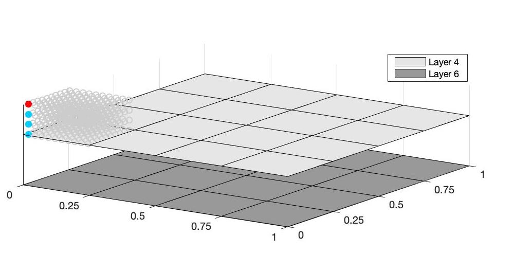
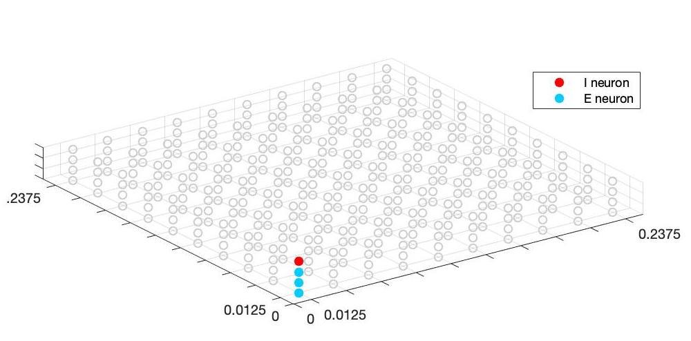
Figure 1. Left: Layout of Model II. Each layer consists of $4\times 4$ hypercolumns. Right: Geometry of each hypercolumn. Each lattice point is occupied by 3 excitatory neurons and 1 inhibitory neuron.

Model III. Then we add orientation columns into the model in order to model two layers in the primary visual cortex. More precisely, each hypercolumn in Model II is further divided into four orientational columns that resembles the pinwheel structure [12, 13, 14]. The layout of orientational columns is demonstrated in Figure 2. We assume the visual stimulation is vertical. The external drive rates to orientational columns with preferences $0$ deg, $45$ deg, $90$ deg, and $135$ deg are multiplied by coefficient $1.0$, $0.6$, $0.2$, and $0.6$ respectively.

We also add long-range excitatory connections on the feedback layer that hits neurons with same orientation preference, with is consistent with experimental studies [26, 8, 20] that many connections are between neurons with the same orientation preferences. The connection probability is given by a linear function. For a pair of neurons $i,j\in\mathcal{ID}$, the probability of having long range connection is

$$p_{Q_{i}Q_{j}}C_{long}(1-0.5d),$$

if $Q_{i}=E$, $d>2L_{EE}$, and neuron $i,j$ have the same orientation preference, where the baseline connection probability $p_{Q_{i}Q_{j}}$ is the same as before, $d$ is the distance between the two neurons in question, and $C_{long}$ is a changing parameter that controls the strength of long range connections. Here we assume that the probability of having long range connections decreases linearly and becomes zero if $d$ is larger than $2$ mm.

Other configurations of Model III are identical to those of Model II.

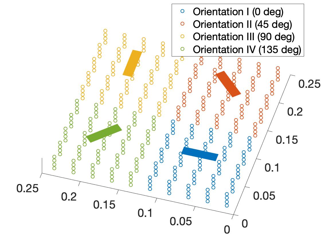
Figure 2. The layout of neurons in one hypercolumn.

2.3. Firing rate and spiking pattern in models

In this subsection we will show some simulation results about our visual cortex models. The first result is about the mean firing rate. Figure 3 gives the firing rate of Model I versus the background drive rate $\lambda^{i}_{E}=\lambda^{i}_{I}=\lambda$ for $i=1,2$ when $\lambda$ increases from $1000$ to $8000$. We can see an increase of empirical firing rate with the background drive. This is consistent with our previous results in [16, 18]. The heat map of firing rates in the most complicated model (Model III) is demonstrated in Figure 4. We can clearly distinguish orientation columns in the heat map. The vertical-preferred orientation columns have highest firing rate, while the horizontal-preferred orientation columns fire the slowest. See caption of Figure 4 for the choice of control parameters.

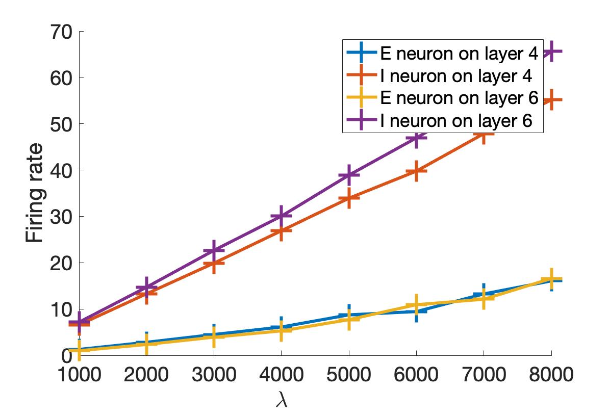
Figure 3. E-population and I-population mean firing rates in layer 4 and 6 when $\lambda$ changes from $1000$ to $8000$. Parameters are $\rho_{f}=\rho_{b}=0.6$, $\tau_{E}=2.0$, $\tau_{I}=4.5$.

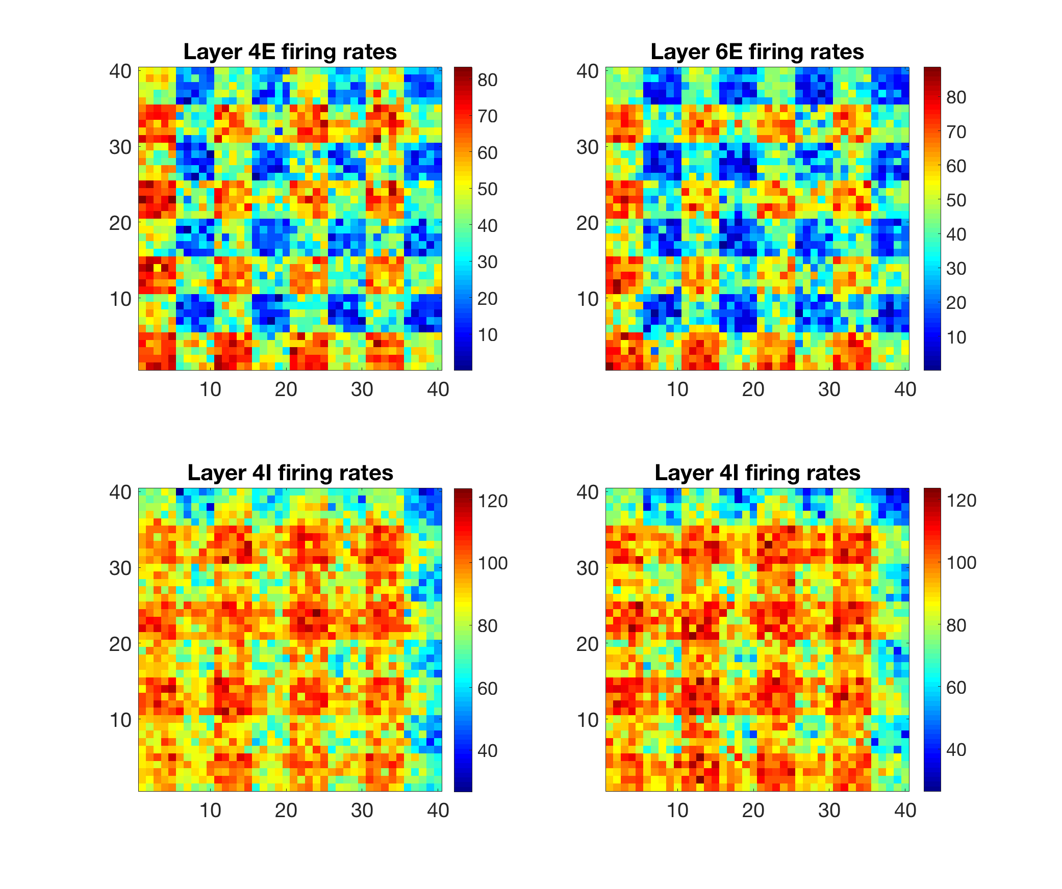
Figure 4. Heat map for E and I firing rates of Model III. Parameters are $\rho_{f}=\rho_{b}=0.6$, $\tau_{E}=2.0$, $\tau_{I}=4.5$.

The spiking pattern is another important feature of spiking neuron models, as neurons pass information through spike trains. Similar as in many pervious studies, the visual cortex models in our study exhibit partial synchronizations. Due to recurrent excitation, neurons tend to form a series of spike volleys, each of which consists of spikes from a proportion of the total population. This phenomenon is known as the multiple firing event (MFE), which is believed to be responsible for the Gamma rhythm [24, 25, 4]. Figure 5 demonstrates the raster plot produced by Model I. We can see obvious MFEs that lie between homogeneous spiking activities and full synchronizations. In addition, the main control parameter of MFE sizes is the ratio $\tau_{I}/\tau_{E}$. Higher $\tau_{I}$-to-$\tau_{E}$ ratio is responsible for more synchronized spike activities. The mechanism of the dependence of MFE sizes on the synapse delay time is addressed in [18]. Slower $\tau_{I}$ means E-cascade can last longer time, which contributes to larger MFE sizes. In Figure 6, we can see raster plots of $(2,2)$ hypercolumn in the feedforward and feedback layer produced by Model II. Top and bottom plots are the cases with and without synapse connections between these two layers, respectively. When the feedforward and feedback connection is turned on, one can see some correlations between MFEs. Later we will use mutual information to quantify such correlation.

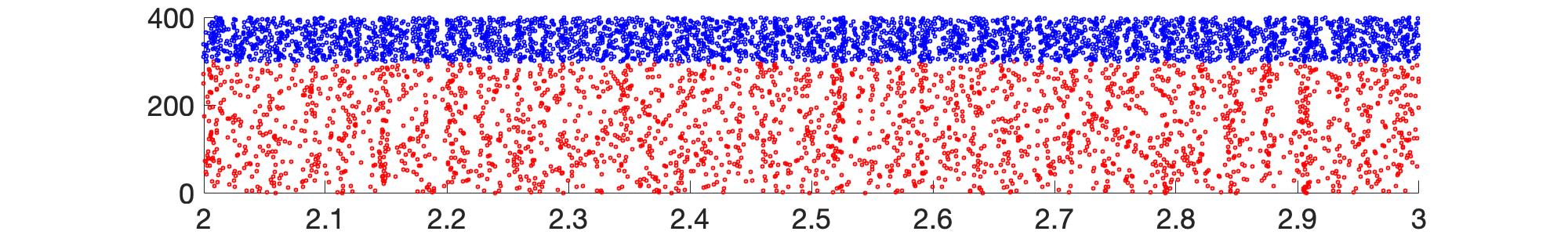
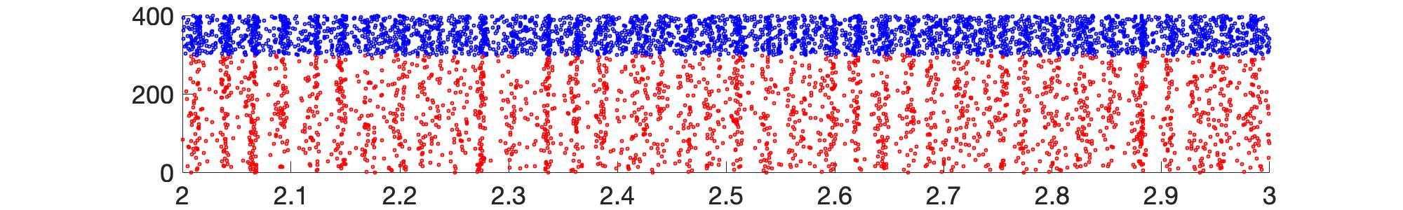
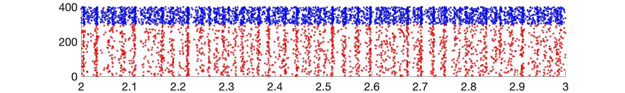
Figure 5. Three raster plots for layer 4 of Model I without feedforward or feedback connection. Top: $\tau_{E}=4.5$ ms, $\tau_{I}=4.5$ ms. Middle: $\tau_{E}=2.0$ ms, $\tau_{I}=4.5$ ms. Bottom: $\tau_{E}=0.9$ ms, $\tau_{I}=4.5$ ms.

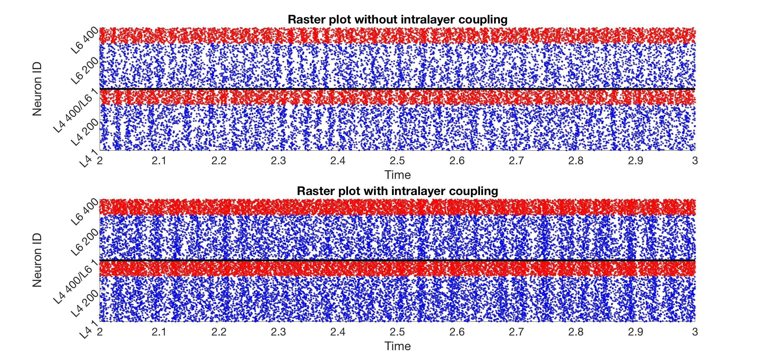
Figure 6. Top. Two raster plots for the (2,2) hypercolumn in layer 4 (top) and the same hypercolumn in layer 6 (bottom). $\rho_{b}=\rho_{f}=0$. $\tau_{E}=2.0$ ms, $\tau_{I}=4.5$ ms. Time span 2-3s. b. Same parameters but with intra-layer connections $\rho_{b}=\rho_{f}=0.6$.

3. Coarse-grained entropy and law of large numbers

3.1. Coarse-grained entropy and coarse-grained information theoretic measures.

Let $T>0$ be a time window size that is associated to a coarse-grained information theoretic measure. Let

$$\mathcal{SP}=\{(t_{i},\xi_{i})\,|\,t_{i}\in\mathbb{R}_{+},\xi_{i}\in\mathcal{ID}\}$$

be the configuration space of neuron spikes, where $i$ is the index of a spike, $t_{i}$ is the time of a spike, and $\xi_{i}$ is the index of the spiking neuron. Let $S_{[0,T])}=(s_{1},\cdots,s_{Z})$ be a spike train produced by $X_{t}$ within the time window $[0,T)$, where $s_{i}\in\mathcal{SP}$ denotes the $i$-th spike within this time window. $Z$ is a random variable that represents the total spike count on $[0,T)$. Let

$$\mathcal{SPT}=E\cup\bigcup_{n\geq 1}\mathcal{SP}^{n}$$

be the configuration space of neural spike trains, where $E$ represents an empty spike train, and $\mathcal{SP}^{n}$ is the $n$-product set of $\mathcal{SP}$. Finally, we let $\mathbf{D}=\{1,2,\cdots,\Sigma\}$ be a dictionary set that consists of countably many distinct integers $1,\cdots,\Sigma$. ($\Sigma$ could be infinity.) A function $\zeta:\mathcal{SPT}\rightarrow\mathbf{D}$ is a coarse-grained mapping that maps a spike train to an element in $\mathbf{D}$. For example, the simplest coarse-grained function is the number of spikes of $X_{t}$ on the interval $[0,T)$. In this case we have $\Sigma=\infty$.

For $i\in\mathbf{D}$, let

$$p_{i}=\mathbb{P}_{\pi}[\zeta(S_{[0,T)})=i]$$

be the probability that the coarse-grained function maps a spike train $S_{[0,T)}$ to $i$ when starting from the invariant probability measure $\pi$. The coarse-grained entropy with respect to $T$ and $\zeta$ is

$$H_{T,\zeta}=-\sum_{i\in\mathbf{D}}p_{i}\log p_{i}\,.$$

If there are $q$ coarse-grained functions $\zeta_{1},\cdots,\zeta_{q}$ and a function $F:\mathbb{R}^{q}\rightarrow\mathbb{R}$, an information theoretical measure $\mathfrak{M}$ with respect to $T$, $\zeta_{1},\cdots,\zeta_{q}$, and $F$ is given by

$$\mathfrak{M}=F(H_{T,\zeta_{1}},\cdots,H_{T,\zeta_{q}})\,.$$

Remark 3.1.

The reason of defining the coarse-grained entropy is to make entropy and information theoretical measures computable. The classical definition of neural entropy can only allow at most one spike in each bin (time window). In a large neural network, neuronal activities are usually synchronized in some degree. As a result, the necessary time window size quickly becomes too small to be practical.

The main simplification we made is to ignore the order of spikes that are sufficiently close to each other. Needless to say this treatment loses some information. But it makes information theoretical measures more computable for large networks. In addition, we map a spike train within a time window to an integer to further reduce the state space. This is because the state space of naive spike counting is still huge. If we naively count the spikes in each hypercolumn in a model with $K$ local populations, there will be $(N_{E}+N_{I})^{K}$ possible spike counting results even if we assume a neuron cannot spike twice in a time bin.

The definition of the coarse-grained entropy is very general. In practice, the function $\zeta$ can be given in the following ways to address different features of the neuronal network.

• Spike counting for a certain local population. If we are interested in the information produced by a certain local population, say local population $k$, we can have

  $$\zeta(S_{[0,T)})=\zeta\left(\{(t_{1},\xi_{1})\cdots,(t_{Z},\xi_{Z})\}\right)=\sum_{j=1}^{Z}\mathbf{1}_{\{\mathrm{Label}_{\xi_{j}}(1)=k\}}\,,$$

  where $\mathrm{Label}_{\xi_{j}}(1)$ means the first entry of $\mathrm{Label}_{\xi_{j}}$, which is the index of the local population of spike $j$. Here one can replace $k$ by either a set of local populations, or restrict on a certain type of neurons.

• Coarse-grained spike counting. If the state space of spike counting is too big to estimate accurately, we can introduce a partition function $\Theta:\mathbb{Z}_{\geq 0}\rightarrow\{1,\cdots,d\}$, such that $\Theta(n)=i$ if $a_{i}\leq n<a_{i+1}$, where $0=a_{0}<a_{1}<\cdots<a_{d+1}=\infty$ is a given sequence of numbers called a “dictionary”. Then let

  $$\zeta(S_{[0,T)})=\Theta\left(\sum_{j=1}^{Z}\mathbf{1}_{\{\mathrm{Label}_{\xi_{j}}(1)=k\}}\right)\,.$$

• Spike counting with delays. If one would like to address time lags of spike activities, the time window $[0,T)$ can be further evenly divided into many sub-windows $[0,T/m),[T/m,2T/m),\cdots,[(m-1)T/m,T)$. Assume we still adopt the coarse grained spike counting in B, we have

  $$\zeta(S_{[0,T)})=\sum_{l=0}^{m-1}d^{l}\Theta\left(\sum_{j=1}^{Z}\mathbf{1}_{\{\mathrm{Label}_{\xi_{j}}(1)=k,t_{j}\in[lT/m,(l+1)T/m)\}}\right)\,.$$

  In other words we take consideration of spike counts in each sub-windows. Integer $m$ is said to be the “word length”.

3.2. Stochastic stability and law of large numbers.

The aim of this section is to prove the law of large numbers holds for entropy. In other words the entropy is computable by running Monte Carlo simulations. To do so, we first need to show the stochastic stability of $X_{t}$.

Let

$$U(\mathbf{x})=1+\sum_{i\in\mathcal{ID}}(H_{i}^{E}+H_{i}^{I})$$

be a function on $\mathbf{\Omega}$. For any signed distribution $\mu$ on the Borel $\sigma$-algebra of $\Omega$, let

$$\|\mu\|_{U}=\sum_{\mathbf{x}\in\mathbf{\Omega}}U(\mathbf{x})|\mu(\mathbf{x})|$$

be the $U$-weighted total variation norm, and let

$$L_{U}(\Omega)=\{\mu\mbox{ on }\mathbf{\Omega}\,|\,\|\mu\|_{U}<\infty\}$$

be the collection of probability distributions with finite $U$-norm. In addition, for any function $\eta(\mathbf{x})$ on $\Omega$, denote

$$\sup_{\mathbf{x}\in\Omega}\frac{|\eta(\mathbf{x})|}{U(\mathbf{x})}$$

by the $U$-weighted supremum norm.

Theorem 3.2.

$X_{t}$ admits a unique invariant probability distribution $\pi\in L_{U}(\mathbf{X})$. In addition, there exists positive constants $c_{1},c_{2}$ and $\gamma\in(0,1)$ such that

$$\|\mu_{1}P^{t}-\mu_{2}P^{t}\|_{U}\leq c_{1}\gamma^{t}\|\mu_{1}-\mu_{2}\|_{U}$$

for any $\mu_{1},\mu_{2}\in L_{U}(\Omega)$ and

$$\|P^{t}\eta-\pi(\eta)\|_{U}\leq c_{2}\gamma^{t}\|\eta-\pi(\eta)\|_{U}$$

for any test function $\eta$ with $\|\eta\|_{U}<\infty$.

We skip the proof of Theorem 3.2 here because it is almost identical to that of Theorem 3.1 in [18]. The only difference is that postsynaptic neurons in the model of [18] is chosen randomly after a spike, which does not affect the proof. To prove the existence of an invariant probability measure $\pi$ and the exponential convergence to it, we need to construct a Lyapunov function $U(\mathbf{x})$ such that

$$P^{h}U\leq\gamma U+K$$

for some $h>0$, $\gamma\in(0,1)$ and $K<\infty$. In addition the “bottom” of $U$, denoted by $C=\{\mathbf{x}\in\Omega\,|\,U(\mathbf{x})\leq R\}$ for some $R>2K(1-\gamma)^{-1}$, must satisfies the minorization condition, which means there exists a constant $\alpha>0$ and a probability distribution on $\Omega$, such that $P^{h}(\mathbf{x},\cdot)\geq\alpha\nu(\cdot)$ uniformly for $\mathbf{x}\in C$. Then the existence and uniqueness of $\pi$ and the exponential speed of convergence to $\pi$ follows from [18]. We refer the proof of Theorem 3.1 in [18] for the full detail.

The next Theorem is about the computability of information-theoretical measures. The way of estimating $H_{T,\zeta}$ is called “plug-in estimate”, which is known to convergence if the spike train $S_{[0,T)}$ is i.i.d. sampled from a certain given probability distribution [1] (also see [23]). However, in our case $S_{[0,T)}$ is the spike count generated by a Markov chain, which depends on the sample path of $X_{t}$ on $[0,T]$. Therefore, one needs to sample $S_{[0,T)}$ by running $X_{t}$ over many time intervals $[0,T),[T,2T),\cdots$. Hence the result in [1] does not apply directly. Instead, we need to use the concept of sample path dependent observable to show that $H_{T,\zeta}$ is a computable quantity.

Theorem 3.3.

Let $\mathcal{T}=NT$ be the length of a trajectory of $X_{t}$. For any coarse-grained mapping $\zeta$ and any $i\in\mathbf{D}$, denote the empirical probability of $\zeta=i$ by

$$\hat{p}_{i}=\frac{1}{N}\sum_{j=1}^{N}\mathbf{1}_{\{\zeta(S_{[(j-1)T,jT)})=i\}}(X_{t})\,.$$

We have

$$\lim_{N\rightarrow\infty}\hat{p}_{i}=\mathbb{P}_{\pi}[\zeta(S_{[0,T)})=i]=p_{i}\,.$$

Proof.

The proof of this theorem relies on the concept of Markov sample path dependent observables. Let $X_{t}$ be a Markov process. A function $Y$ is said to be a Markov sample-path dependent observable on an interval $[t_{1},t_{2})$ if

1. $Y$ is a real-valued function on $C_{\Omega}([t_{1},t_{2}))$, where $C_{\Omega}([t_{1},t_{2}))$ is the collection of cadlag paths from $t_{1}$ to $t_{2}$ on $\Omega$.

2. The law of $Y$ only depends on the value of $X_{t_{1}}$.

Now let $Y_{1},Y_{2},\cdots,Y_{n},\cdots$ be a sequence of sample-path dependent observables on $[0,T)$, $[T,2T)$, $\cdots$, $[(n-1)T,nT)$ respectively. Since the law of $X_{t}$ converges to $\pi$ as $t\rightarrow\infty$, by Theorem 3.3 in [18], we have the law of large numbers for $\{Y_{n}\}$, i.e.,

$$\lim_{N\rightarrow\infty}\frac{1}{N}\sum_{n=1}^{N}Y_{n}=\mathbb{E}_{\pi}[Y_{1}]$$

provided there exists a constant $M<\infty$, such that $\mathbb{E}[Y^{2}_{n}\,|\,X_{(n-1)T}=\mathbf{x}]<M$ uniformly for all $\mathbf{x}\in\mathbf{\Omega}$.

Hence we only need to construct a sequence of sample-path dependent observables $\{Y_{n}\}$ whose expectations equal to $\hat{p}_{i}$. Let

$$Y_{n}=\mathbf{1}_{\{\zeta(S_{[(n-1)T,nT)})=i\}}\,.$$

It is easy to see that $Y_{n}$ is Markov because $X_{t}$ is a Markov process. In addition, $\mathbb{E}[Y_{n}^{2}]\leq 1$ uniformly because $Y_{n}$ is a indicator function. Therefore, $\{Y_{n}\}_{n=1}^{\infty}$ satisfies the law of large numbers. This completes the proof.

∎

3.3. Numerical result and discussion

We did the following two numerical simulations to demonstrate the role of coarse-grained entropy in our network models. Consider model I without feedforward or feedback connections. Without loss of generality we only compute the entropy of the feedforward layer. The synapse delay times are chosen to be $\tau_{E}=2$ ms and $\tau_{I}=4.5$ ms.

The first test is about the entropy rate per second with increasing word length. We use spike counting with delays to define the coarse-grained mapping $\zeta$ (case C in Section 3.1). The duration of each sub-window is $T/m=5$ ms. The time window size goes through $T=5$ ms (m=1) to $T=60$ ms (m = 12). Then we define the partition function $\Theta:\mathbf{Z}_{+}\rightarrow\{0,1,2,3\}$ with $\Theta(n)=0$ for $n<4$, $\Theta(n)=1$ for $4\leq n<8$, $\Theta(n)=2$ for $8\leq n<12$, and $\Theta(n)=3$ for $n\geq 12$. Figure 7 shows the entropy rate (entropy divided by the time window size) versus time window size. The curve is similar to that given in [28]. Starting from word length $=2$, and until the word length being too long for estimating entropy, the entropy rate declines linearly. But when a “word” is too long such that the entropy estimation is badly under-sampled, the estimated entropy rate declines faster-than-linear, as explained in [28]. We use extrapolation to estimate the entropy rate at the infinite window size limit, as shown in Figure 3 of [28].

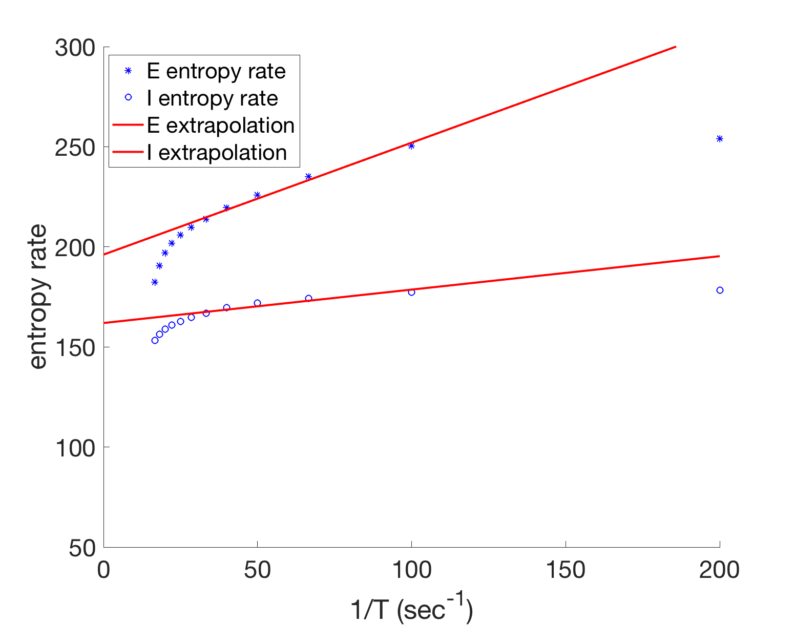
Figure 7. Entropy rate versus time window length. Samples are collected from eight trajectories with length $10000$. Linear extrapolation uses points with respect to $m=2,3,\cdots,7$.

The second test is the entropy for different degrees of synchrony. Here we only consider word length $=1$ with time window size $T=15$ ms, with a more refined partition function $\Theta:\mathbb{Z}_{+}\rightarrow\{0,1,\cdots,45\}$ such that $\Theta(n)=i$ for $3i\leq n<3(i+1)$ if $i=0,\cdots,44$ and $\Theta(n)=45$ if $n\geq 135$. The excitatory synapse delay time is set to be $\tau_{I}=4.5$ ms. And $\tau_{I}$-to-$\tau_{E}$ ratio varies between $0.5$ and $3.5$. In addition we let $S_{EE}=6$ to increase the degree of synchrony. The entropy rate versus $\tau_{I}/\tau_{E}$ is plotted in Figure 8. We can see that the entropy reaches a peak in the middle of the tuning curve for both E and I neurons. The peak locations are different for E and I neurons partially due to different population sizes. The heuristic reason is straightforward. When $\tau_{I}/\tau_{E}$ is small, the spiking pattern is homogeneous, and the distribution of spike counts in each time window concentrates at a few small numbers. Larger $\tau_{I}/\tau_{E}$ means larger MFE sizes, which makes spike counts in each time window more diverse. But when $\tau_{I}/\tau_{E}$ is too large and such that all MFEs are large, such diversity shows slight decreases. In other words, our simulation shows that the partial synchronization, rather than the full synchronization, helps a neuronal network to produce more information.

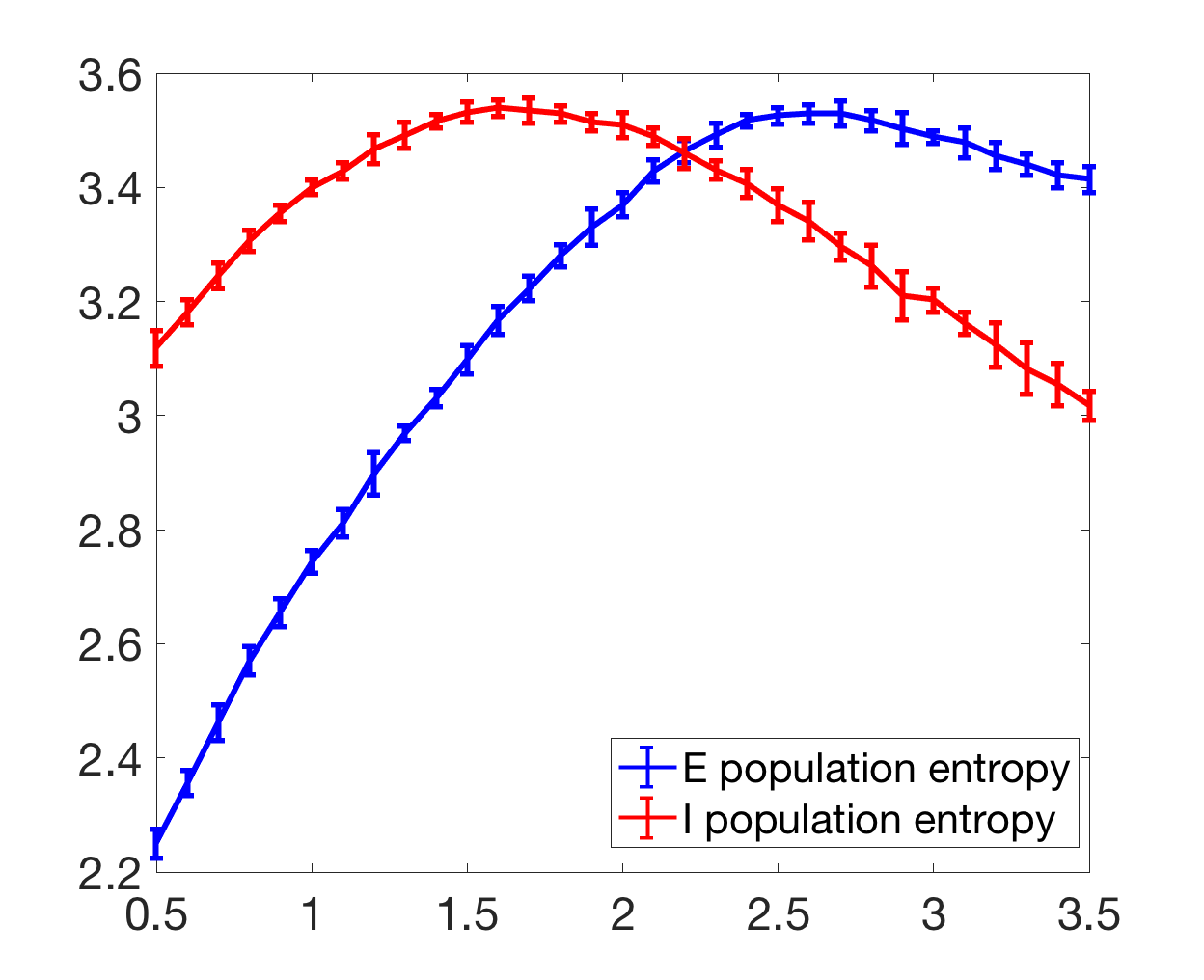
Figure 8. Entropy versus delay time for Model I. Each simulation runs up to $\mathcal{T}=50$.

4. Mutual information

4.1. Mutual information and conditional mutual information

Based on the framework of spike train space defined in Section 3.1, one can also define the mutual information. Let $T>0$ be a fixed time window size. A coarse-grained function $\mathcal{SPT}\rightarrow\mathbf{D}$ with respect population set $C\subset\{1,\cdots,K\}$ is denoted by $\zeta_{C}$ if it gives joint spike count distributions from populations that belong to $C$. Here $C=\{C_{1},\cdots,C_{|C|}\}$ is a generic subset of $\{1,\cdots,K\}$. We have

(4.1) $$\zeta_{C}(S_{[0,T]})=\sum_{n=1}^{|C|}d^{n-1}\left(\Theta\left(\sum_{j=1}^{Z}\mathbf{1}_{\{\mathrm{Label}_{\xi_{j}}(1)\in C_{n}\}}\right)\right)\,,$$

where $\mathrm{Label}_{\xi_{j}}(1)$ means the first entry (index of local population) of $j$-th spiked neuron, and $\Theta:\mathbb{Z}_{\geq 0}\rightarrow\{1,\cdots,d\}$ is a partition function that maps a spike count to an integer. Here the definition of $\zeta_{C}$ can also be extended to the case of a particular type of neurons, or the case of spike counts with delays.

Now consider two disjoint sets of local populations $A,B\subset\{1,\cdots,K\}$. The mutual information is an information theoretical measure that is given by

$$\mathrm{MI}_{T,\zeta}(A:B)=H_{T,\zeta_{A}}+H_{T,\zeta_{B}}-H_{T,\zeta_{A\cup B}}\,.$$

In other words, the mutual information measures the information shared by populations in $A$ and populations in $B$ when the spike count is measured by the coarse-grained map $\xi$.

The coarse-grained mutual information $\mathrm{MI}_{T,\zeta}(A:B)$ is the mutual information between two spike trains produced by local populations $A$ and $B$ that are processed by coarse-grained function $\zeta_{A}$ and $\zeta_{B}$ respectively. By the data processing inequality [6], $\mathrm{MI}_{T,\zeta}(A:B)$ is no greater than the actual mutual information between two unprocessed spike trains on $A$ and $B$ respectively. Therefore, the “true” mutual information is larger than our measurement by using coarse-graining functions.

4.2. Mutual information in visual cortex models

The following simulations aim to use mutual information to study the correlation in our visual cortex models. We present the following $4$ results.

Simulation I: Role of feedforward and feedback. In this study we first consider Model I, which is a the feedforward-feedback network with only two local populations. We let the time window size be $10$ ms with word length $=1$. The partition function $\Theta$ maps $\mathbb{Z}_{+}$ to $\{0,1,\cdots,10\}$ such that $\Theta(n)=i$ for $5i\leq n<5(i+1)$ if $i=0,1,\cdots,9$ and $\Theta(n)=10$ if $n\geq 50$. The mutual information between the feedforward layer and the feedback layer versus the coupling strength is plotted in Figure 9 Left. We consider three cases: (i) $\rho_{f}=\rho_{b}=\rho$, (ii) $\rho_{f}=\rho,\rho_{b}=0$, and (iii) $\rho_{f}=0,\rho_{b}=\rho$. One can see a clear increase of mutual information between two layers with increasing coupling. And the presence of both feedforward and feedback connection can significantly increase the mutual information between two layers. This is somehow expected: communications between neuronal networks can increase the information shared between them. The same simulation is done in Model II, which has many hypercolumns and geometric structures. The mutual information is measured between $(2,2)$ hypercolumn of layer 4 and $(2,2)$ hypercolumn of layer 6. The corresponding partition function for Model II is $\Theta(n)=i$ for $10i\leq n<10(i+1)$ if $i=0,1,\cdots,9$ and $\Theta(n)=10$ if $n\geq 100$. All other parameters are same as those in Model I. The result is plotted in Figure 9 Right. We can see the same pattern as in Figure 9 Left. Note that when $\rho_{f}=0,\rho_{b}=\rho$ and $\rho$ is very large, the network becomes almost fully synchronized. The mutual information slightly decreases in this regime because the entropy decreases in a very synchronized network, as seen in Figure 8.

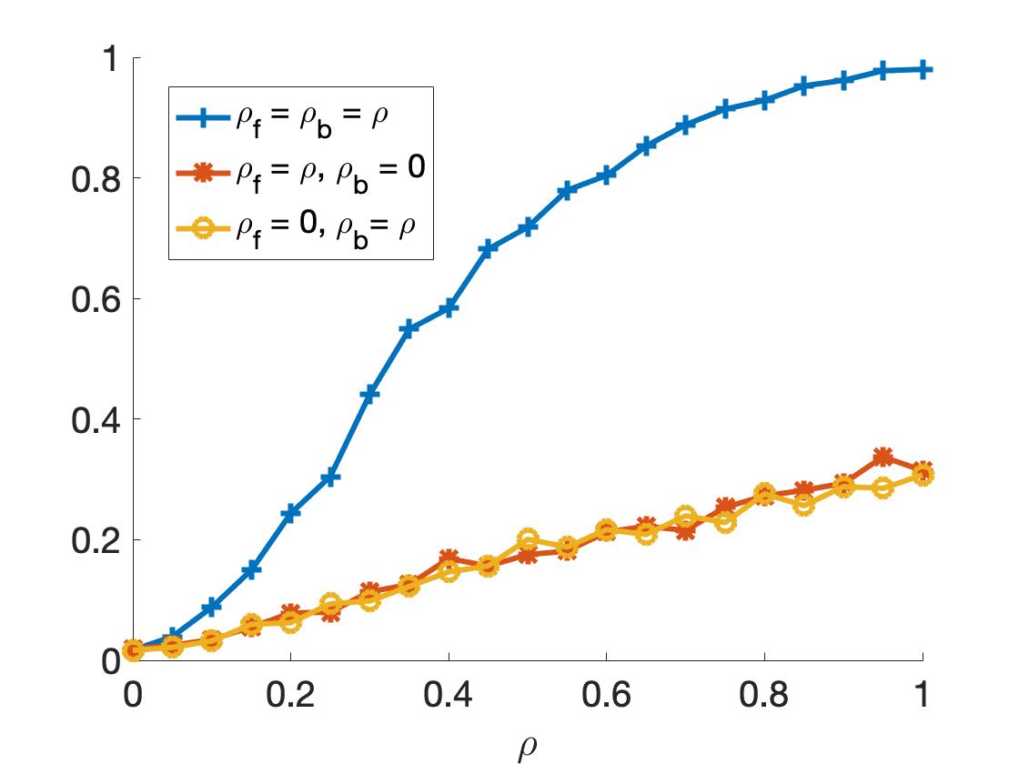
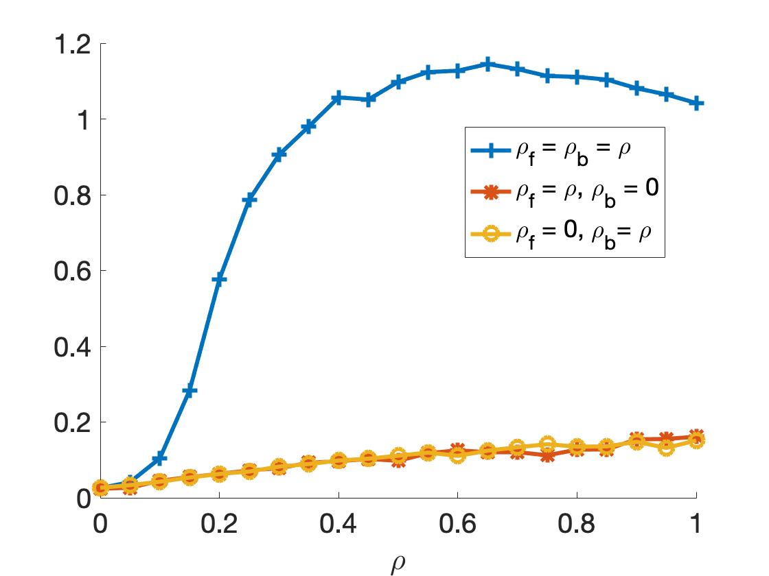
Figure 9. Mutual information versus coupling strength for Model I (left) and Model II (right).

Simulation II: Mutual information versus distance. The second simulation considers the dependence of mutual information on the distance between two hypercolumns. We fix the coupling strength as $\rho_{f}=\rho_{b}=0.6$ and study mutual information between hypercolumns for model II and model III. In Figure 10 Top, mutual information between $(1,1)$ hypercolumn and all other hypercolumns are demonstrated for model II. Model III has orientational columns. In Figure 10 Bottom, we show the mutual information between the vertical-preferred orientation column in $(1,1)$ hypercolumn and all other orientation columns in model III. The logarithmic scale is used because the entropy at the bottom left corner is much larger than all mutual information. We can clearly see a decrease of mutual information with increasing distance. This is consistent with our results in [18] that correlation of MFE sizes decays quickly with the distance. The fast decline of mutual information is also supported by experimental evidence. It is known that MFEs are responsible for the Gamma rhythm in the cortex, which is known to be local in many scenarios [9, 15, 21]. In addition, in Figure 10 Bottom, we can also see that orientation columns with the same preferred orientations share higher mutual information than those with opposite preferred orientations.

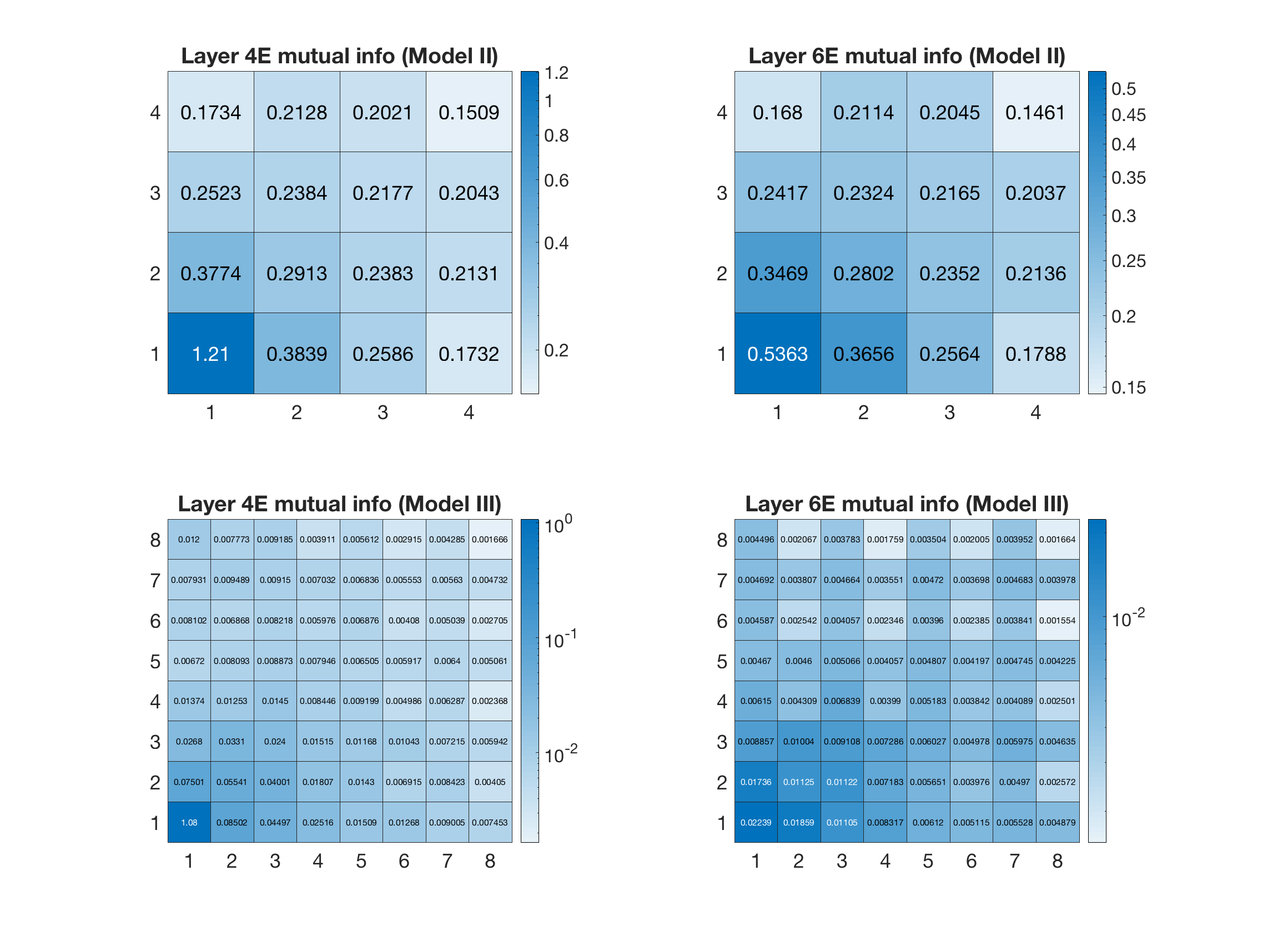
Figure 10. Top: heat map of mutual information with $(1,1)$ hypercolumn in Model II. Top left: Layer 4. Top right: Layer 6. Bottom: heat map of mutual information with vertical-preferred orientation column in $(1,1)$ hypercolumn in Model III. Bottom left: Layer 4. Bottom right: Layer 6.

5. Systematic measures: degeneracy and complexity

5.1. Definitions and rigorous results.

As introduced in the introduction, systematic measures, including degeneracy, complexity, redundancy, and robustness, are first proposed in the study of systems biology. When a biological network is too large to be investigated in full detail, systematic measures are used to describe the global characteristics of the network. In [29, 17], degeneracy and complexity are quantified as linear combinations of mutual information. This section uses the idea of coarse-grained entropy to define two systematic measures, i.e., degeneracy and complexity, for a spiking neuronal network. The case of other systematic measures like the redundancy [29] can be studied analogously.

The definition of degeneracy and complexity relies on multivariate mutual information. Still consider a neuronal network with $K$ local populations. Let $\zeta_{I}$ be a coarse-grained function with respect to $I\subset\{1,\cdots,K\}$. For three sets $A,B,C\subset\{1,\cdots,K\}$, the multivariate mutual information $MI(A:B:C)$ is given as

$$MI_{T,\zeta}(A:B:C) = MI_{T,\zeta}(A:C)+MI_{T,\zeta}(B:C)-MI_{T,\zeta}(A\cup B:C)$$

$$= H_{T,\zeta_{A}}+H_{T,\zeta_{B}}+H_{T,\zeta_{C}}-H_{T,\zeta_{A\cup B}}-H_{T,\zeta_{B\cup C}}-H_{T,\zeta_{A\cup C}}+H_{T,\zeta_{A\cup B\cup C}}\,.$$

The following proposition follows immediately from the definition of multivariate mutual information.

Proposition 5.1.

• If $\zeta_{A}(S_{[0,T)})$, $\zeta_{B}(S_{[0,T)})$, and $\zeta_{C}(S_{[0,T)})$ are identical random variables, then $MI_{T,\zeta}(A:B:C)=H_{T,\zeta_{A}}$.

• If $\zeta_{A}(S_{[0,T)})$, $\zeta_{B}(S_{[0,T)})$ are independent from $\zeta_{C}(S_{[0,T)})$, then $MI_{T,\zeta}(A:B:C)=0$.

Proof.

If all three random variables are equal, we have

$$H_{T,\zeta_{A\cup B}}=H_{T,\zeta_{A}}$$

because the histogram of $\zeta_{A\cup B}(S_{[0,T)})$ is supported by the diagonal set, which equals $\zeta_{A}(S_{[0,T)})$. Similar argument implies that

$$H_{T,\zeta_{B\cup C}}=H_{T,\zeta_{A\cup C}}=H_{T,\zeta_{A\cup B\cup C}}=H_{T,\zeta_{A}}\,.$$

This implies (a).

If $\zeta_{C}(S_{[0,T)})$ is independent of $\zeta_{A}(S_{[0,T)}),\zeta_{B}(S_{[0,T)})$, we have

$$H_{T,\zeta_{B\cup C}}=H_{T,\zeta_{B}}+H_{T,\zeta_{C}},\quad H_{T,\zeta_{A\cup C}}=H_{T,\zeta_{A}}+H_{T,\zeta_{C}}$$

and

$$H_{T,\zeta_{A\cup B\cup C}}=H_{T,\zeta_{A\cup B}}+H_{T,\zeta_{C}}\,.$$

It follows from equation (LABEL:MMI) that

$$MI_{T,\zeta}(A:B:C)=MI_{T,\zeta}(A:B)-MI_{T,\zeta}(A:B)=0\,.$$

∎

Now consider a neuronal network with $K$ local populations. Let two disjoint sets $\mathcal{I},\mathcal{O}\subset\{1,\cdots,K\}$ denote the input set and output set of this network. The degeneracy $\mathcal{D}_{T,\zeta}(\mathcal{I}:\mathcal{O})$ is given by the weighted sum of multivariate mutual informations:

(5.2) $$\mathcal{D}_{T,\zeta}(\mathcal{I}:\mathcal{O})=\sum_{0\leq k\leq|\mathcal{I}|}\frac{1}{2{|\mathcal{I}|\choose k}}MI_{T,\zeta}(\mathcal{I}_{k}:\mathcal{I}_{k}^{c}:\mathcal{O})\,,$$

where the summation goes through all possible partitions of $\mathcal{I}$. Set $\mathcal{I}_{k}$ means a subset of $\mathcal{I}$ with $k$ local populations. Degeneracy measures how much more information different components of the input set share with the output set than expected if all components are independent. Degeneracy is high if many structurally different components in the input set can perform similar functions on a designated output set. A neuronal network is said to be degenerate if $\mathcal{D}_{T,\zeta}(\mathcal{I}:\mathcal{O})>0$ for some choice of $T,\zeta,\mathcal{I}$, and $\mathcal{O}$.

The (structural) complexity $\mathcal{C}_{T,\zeta}(\mathcal{I}:\mathcal{O})$ is given by the weighted sum of mutual information between components of the input set.

(5.3) $$\mathcal{C}_{T,\zeta}(\mathcal{I}:\mathcal{O})=\sum_{0\leq k\leq|\mathcal{I}|}\frac{1}{2{|\mathcal{I}|\choose k}}MI_{T,\zeta}(\mathcal{I}_{k}:\mathcal{I}_{k}^{c})\,,$$

The complexity measures how much codependency in a network appears among different components of the input set. Again, a neuronal network is said to be (structurally) complex if $\mathcal{C}_{T,\zeta}(\mathcal{I}:\mathcal{O})>0$ for some choice of $T,\zeta,\mathcal{I}$, and $\mathcal{O}$.

The degeneracy at two limit cases can be given by proposition 5.1 easily. When the input is independent of the output, we have zero degeneracy. When a neuronal network is fully synchronized, and $A,B,C$ are three local populations with $\mathcal{I}=\{A,B\},\mathcal{O}=C$, then the degeneracy equals to $H_{\zeta,T}(A)$, which is positive. Our numerical simulation result will confirm this.

Finally, we have the following lemma regarding the connection between degeneracy and complexity.

Lemma 5.2.

For any choice of $T,\zeta,\mathcal{I}$, and $\mathcal{O}$ and any decomposition $\mathcal{I}=\mathcal{I}_{k}+\mathcal{I}_{k}^{c}$, we have

$$MI_{T,\zeta}(\mathcal{I}_{k}:\mathcal{I}_{k}^{c}:\mathcal{O})\leq\min\{MI_{T,\zeta}(\mathcal{I}_{k}:\mathcal{I}_{k}^{c}),MI_{T,\zeta}(\mathcal{I}_{k}:\mathcal{O}),MI_{T,\zeta}(\mathcal{I}_{k}^{c}:\mathcal{O})\}\,.$$

Proof.

This lemma is a discrete version of Lemma 5.1 of [19]. We include it for the sake of completeness of this paper. It is sufficient to prove that for any three discrete random variables $X$, $Y$, and $Z$ with joint probability distribution function $p(x,y,z)=\mathbb{P}[X=x,Y=y,Z=z]$,

$$MI(X:Y:Z)\leq\min\{MI(X:Y),MI(X:Z),MI(Y:Z)\}\,.$$

It follows from the definition of the multivariate mutual information and some elementary calculations that

$$MI(X:Y:Z) = H(X)+H(Y)+H(Z)-H(X,Y)-H(X,Z)-H(Y,Z)+H(X,Y,Z)$$

$$= MI(X:Y)-(H(X,Z)+H(Y,Z)-H(Z)-H(X,Y,Z)$$

$$= MI(X:Y)-MI(X:Y\,|\,Z)\,,$$

where the latter time is the conditional mutual information. The conditional mutual information is nonnegative, as a direct corollary of Kullback’s inequality [31]. Hence

$$MI(X:Y:Z)\leq MI(X:Y)\,.$$

Inequalities $MI(X:Y:Z)\leq MI(X:Z)$ and $MI(X:Y:Z)\leq MI(Y:Z)$ follow analogously. This completes the proof. ∎

The following theorem is a straightforward corollary of Lemma 5.2.

Theorem 5.3.

For any choice of $T,\zeta,\mathcal{I}$, and $\mathcal{O}$,

$$\mathcal{D}_{T,\zeta}(\mathcal{I}:\mathcal{O})\leq\mathcal{C}_{T,\zeta}(\mathcal{I}:\mathcal{O})\,.$$

Heuristically, Theorem 5.3 says that a neuronal network with high degeneracy must has high (structural) complexity as well.

5.2. degeneracy and complexity in a visual cortex model

We consider the following three numerical simulations to measure the degeneracy and complexity in model II and model III. Because the estimation of entropy is not satisfactory when the simulation is under-sampled, we limit the cardinality of $|\mathcal{I}|$ to three and only consider the case of $|\mathcal{O}|=1$

Numerical simulation I. In Model II, we consider the input set $\mathcal{I}=\{L_{6},L_{7},L_{10}\}$ and $\mathcal{O}=L_{22}$. In other words the input set consists of hypercolumns $(2,2),(2,3)$, and $(3,2)$ in layer 4 and the output set is local population $(2,2)$ in layer 6. The synapse delay times are chosen to be $\tau_{E}=2$ ms and $\tau_{I}=4.5$ ms. The time window size is $T=5$ ms. The coarse-grained function $\zeta_{C}$ with respect to a generic set $C$ is given as in equation (4.1), with a partition function $\Theta$ maps $\mathbb{Z}_{+}$ to $\{0,1,2,3,4,5\}$ such that $\Theta(n)=i$ for $20i\leq n<20(i+1)$ if $i=0,1,\cdots,4$ and $\Theta(n)=5$ if $n\geq 100$. Figure 11 Left shows the dependence of degeneracy $\mathcal{D}_{\zeta,T}(\mathcal{I},\mathcal{O})$ versus the coupling strength between layers $\rho_{f}=\rho_{b}=\rho$. We can see that the degeneracy and complexity increases with $\rho$ in general. When $\rho$ is too large, the recurrent excitation cannot be tempered by inhibitions and the network fires at a very high rate that can not be captured by the partition map $\Theta$. As a result, both $\mathcal{D}$ and $\mathcal{C}$ drops to very small values.

Numerical simulation II. Now we take orientation columns into considerations. In Model III, we let the input set $\mathcal{I}$ consist of three orientation columns in hypercolumn $(2,2)$ of layer 4, with orientation preferences $0$ deg, $45$ deg, and $90$ deg respectively. The output set is the orientation column in hypercolumn $(2,2)$ of layer 6, with an orientation preference $0$ deg. The synapse delay times are chosen to be $\tau_{E}=2$ ms and $\tau_{I}=4.5$ ms. The time window size is $T=5$ ms. The coarse-grained function $\zeta_{C}$ is similar as in Numerical simulation I, except the partition function takes value $\Theta(n)=i$ for $10i\leq n<10(i+1)$ if $i=0,1,\cdots,4$ and $\Theta(n)=5$ if $n\geq 50$, because an orientation column contains less neurons than a hypercolumn. The strength of long range connection is given by $C_{long}=0.5$. Figure 11 Middle shows the dependence of degeneracy $\mathcal{D}_{\zeta,T}(\mathcal{I},\mathcal{O})$ versus the coupling strength between layers $\rho_{f}=\rho_{b}=\rho$. Again, stronger coupling between layers leads to larger degeneracy, until the network firing rate is too high to be captured by the given partition function.

Numerical simulation III. The third simulation studies the effect of long range connections. Still in Model III, we let the input set $\mathcal{I}$ consist of three orientation columns with orientation preference $0$ deg in hypercolumns $(2,2),(2,3)$, and $(3,2)$ of layer 4. The output set is the orientation column in hypercolumn $(2,2)$ of layer 6, with an orientation preference $0$ deg. Parameters like the synapse delay times, the time window size, the coarse-grained function $\zeta_{C}$ are identical to those of Numerical simulation II. The feedforward and feedback strengths are $\rho_{b}=\rho_{f}=0.6$. And the strength of long range connections is the main control parameter. Figure 11 shows the dependence of degeneracy $\mathcal{D}_{\zeta,T}(\mathcal{I},\mathcal{O})$ versus the strength of long range connections $C_{long}$. We can see that a stronger long range coupling between orientation columns also leads to a higher degeneracy.

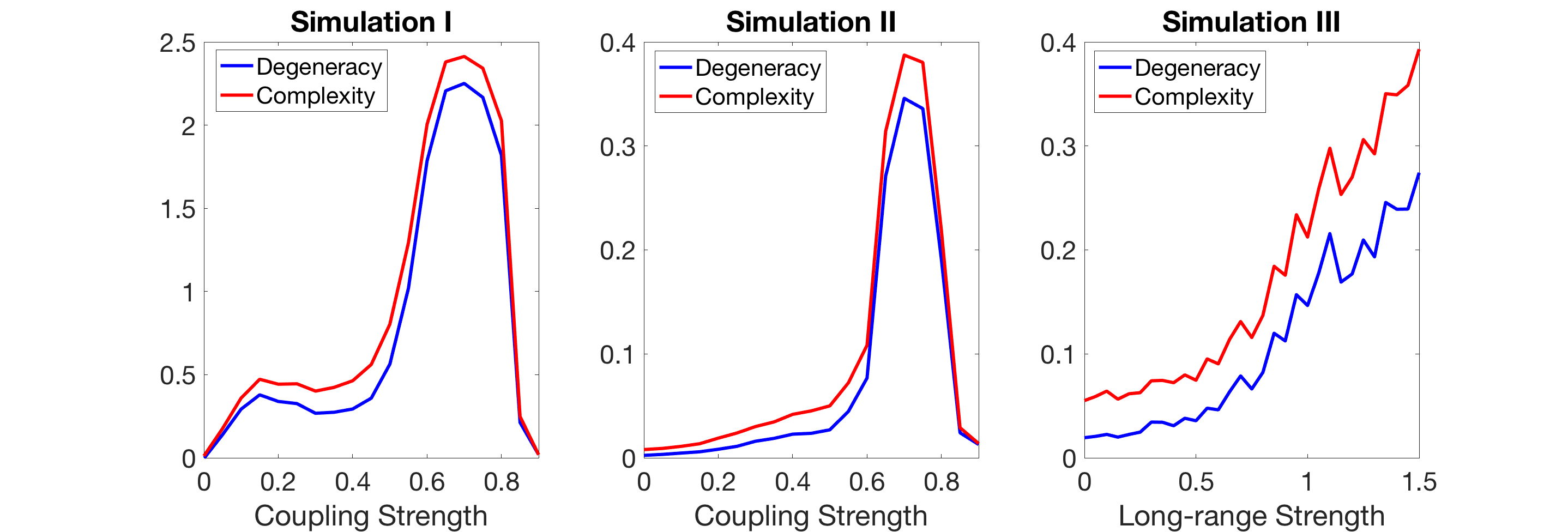
Figure 11. Degeneracy and complexity in model II and III. Left, middle, and right panels are from from Numerical simulation I - III respectively. Length of simulation = 20 with $16$ independent threads.

6. Conclusion

This paper investigates a few information-theoretic measures of a class of structured neuronal networks. Neurons in the network are of the integrate-and-fire type. Being consistent with our earlier papers [16, 18], membrane potentials are set to be discrete to make the model mathematically and computationally simple. The network consists of many local populations, each of which has its own external drive rate. Biologically, one local population could be a hypercolumn in the cortex or an orientational column in the visual cortex. We provided several different network models for the purpose of examining information-theoretic measures. The most complicated model (Model III) aims to model two layers (layer 4 and layer 6) of the primary visual cortex, each layer has $4\times 4$ hypercolumns, each hypercolumn has $4$ orientational columns.

Then we use the idea of coarse-graining to define the coarse-grained entropy. The motivation is that the naive definition of neuronal entropy works poorly for large neuronal networks. One needs unrealistically large sample to estimate the entropy in a trustable way. In addition it is known that many neuronal network can generate Gamma-type rhythms. Hence when calculating the entropy, we chose to ignore the precise order of neuronal spikes from the same local population if they fall into the same small time bin. This entropy mainly captures the uncertain in the oscillations produced by the neuronal network. One can easily compute the entropy for large scale neuronal networks. The mutual information can be defined analogously.

The coarse-grained entropy and the mutual information is examined through our examples. We found that the coarse-grained entropy mainly capture the information contained in the rhythm produced by a local population. Under suitable setting of the partition function, the coarse-grained entropy reaches maximal value when the partial synchronization has the most diversity, and decreases when the spiking pattern is either homogeneous or fully synchronized. Furthermore, in our two-layer network model, we found that stronger connections between layers can produce higher mutual information between layers. This is very heuristic, as stronger coupling between layers makes the firing patterns from two layers more synchronized.

In the end, we attempts to quantify two systematic measures, namely the degeneracy and the complexity, for spiking neuronal network models. These systematic measures are originally proposed in the study of systems biology. They can be written as linear combinations of mutual informations. Therefore, after defining coarse-grained entropy and mutual information, these systematic measures can be defined analogously. We found that the inequality proved in our earlier paper [19] still holds, which says that the degeneracy is always smaller than the complexity, or a system with high degeneracy must be structurally complex. Finally, we numerically computed degeneracy and complexity for our two-layer cortex models. We found that at certain range of parameters, stronger coupling between layers, as well as stronger long-range connectivities, leads to both larger degeneracy and larger complexity.

References

- [1] András Antos and Ioannis Kontoyiannis, Convergence properties of functional estimates for discrete distributions, Random Structures & Algorithms 19 (2001), no. 3-4, 163–193.
- [2] Alexander Borst and Frédéric E Theunissen, Information theory and neural coding, Nature neuroscience 2 (1999), no. 11, 947.
- [3] Logan Chariker, Robert Shapley, and Lai-Sang Young, Orientation selectivity from very sparse lgn inputs in a comprehensive model of macaque v1 cortex, Journal of Neuroscience 36 (2016), no. 49, 12368–12384.
- [4] Logan Chariker and Lai-Sang Young, Emergent spike patterns in neuronal populations, Journal of computational neuroscience 38 (2015), no. 1, 203–220.
- [5] Madalena Costa, Ary L Goldberger, and C-K Peng, Multiscale entropy analysis of biological signals, Physical review E 71 (2005), no. 2, 021906.
- [6] Thomas M Cover and Joy A Thomas, Elements of information theory, John Wiley & Sons, 2012.
- [7] Gerald M Edelman and Joseph A Gally, Degeneracy and complexity in biological systems, Proceedings of the National Academy of Sciences 98 (2001), no. 24, 13763–13768.
- [8] Charles D Gilbert and Torsten N Wiesel, Columnar specificity of intrinsic horizontal and corticocortical connections in cat visual cortex, Journal of Neuroscience 9 (1989), no. 7, 2432–2442.
- [9] C Alex Goddard, Devarajan Sridharan, John R Huguenard, and Eric I Knudsen, Gamma oscillations are generated locally in an attention-related midbrain network, Neuron 73 (2012), no. 3, 567–580.
- [10] Gerald Hahn, Alejandro F Bujan, Yves Frégnac, Ad Aertsen, and Arvind Kumar, Communication through resonance in spiking neuronal networks, PLoS computational biology 10 (2014), no. 8, e1003811.
- [11] Gerald Hahn, Adrian Ponce-Alvarez, Gustavo Deco, Ad Aertsen, and Arvind Kumar, Portraits of communication in neuronal networks, Nature Reviews Neuroscience (2018), 1.
- [12] David H Hubel, Eye, brain, and vision., Scientific American Library/Scientific American Books, 1995.
- [13] Kukjin Kang, Michael Shelley, and Haim Sompolinsky, Mexican hats and pinwheels in visual cortex, Proceedings of the National Academy of Sciences 100 (2003), no. 5, 2848–2853.
- [14] Matthias Kaschube, Michael Schnabel, Siegrid Löwel, David M Coppola, Leonard E White, and Fred Wolf, Universality in the evolution of orientation columns in the visual cortex, science 330 (2010), no. 6007, 1113–1116.
- [15] Kwang-Hyuk Lee, Leanne M Williams, Michael Breakspear, and Evian Gordon, Synchronous gamma activity: a review and contribution to an integrative neuroscience model of schizophrenia, Brain Research Reviews 41 (2003), no. 1, 57–78.
- [16] Yao Li, Logan Chariker, and Lai-Sang Young, How well do reduced models capture the dynamics in models of interacting neurons?, Journal of mathematical biology 78 (2019), no. 1-2, 83–115.
- [17] Yao Li, Gaurav Dwivedi, Wen Huang, Melissa L Kemp, and Yingfei Yi, Quantification of degeneracy in biological systems for characterization of functional interactions between modules, Journal of theoretical biology 302 (2012), 29–38.
- [18] Yao Li and Hui Xu, Stochastic neural field model: multiple firing events and correlations, Journal of mathematical biology (2019), 1–36.
- [19] Yao Li and Yingfei Yi, Systematic measures of biological networks ii: Degeneracy, complexity, and robustness, Communications on Pure and Applied Mathematics 69 (2016), no. 10, 1952–1983.
- [20] R Malach, Y Amir, M Harel, and A Grinvald, Relationship between intrinsic connections and functional architecture revealed by optical imaging and in vivo targeted biocytin injections in primate striate cortex, Proceedings of the National Academy of Sciences 90 (1993), no. 22, 10469–10473.
- [21] V Menon, WJ Freeman, BA Cutillo, JE Desmond, MF Ward, SL Bressler, KD Laxer, N Barbaro, and AS Gevins, Spatio-temporal correlations in human gamma band electrocorticograms, Electroencephalography and clinical Neurophysiology 98 (1996), no. 2, 89–102.
- [22] Ilya Nemenman, William Bialek, and Rob De Ruyter Van Steveninck, Entropy and information in neural spike trains: Progress on the sampling problem, Physical Review E 69 (2004), no. 5, 056111.
- [23] Liam Paninski, Estimation of entropy and mutual information, Neural computation 15 (2003), no. 6, 1191–1253.
- [24] Aaditya V Rangan and Lai-Sang Young, Dynamics of spiking neurons: between homogeneity and synchrony, Journal of Computational Neuroscience 34 (2013), no. 3, 433–460.
- [25] by same author, Emergent dynamics in a model of visual cortex, Journal of Computational Neuroscience 35 (2013), no. 2, 155–167.
- [26] Dan D Stettler, Aniruddha Das, Jean Bennett, and Charles D Gilbert, Lateral connectivity and contextual interactions in macaque primary visual cortex, Neuron 36 (2002), no. 4, 739–750.
- [27] SP Strong, RR De Ruyter Van Steveninck, William Bialek, and Roland Koberle, On the application of information theory to neural spike trains, Pac Symp Biocomput, vol. 1998, 1998, pp. 621–632.
- [28] Steven P Strong, Roland Koberle, Rob R De Ruyter Van Steveninck, and William Bialek, Entropy and information in neural spike trains, Physical review letters 80 (1998), no. 1, 197.
- [29] Giulio Tononi, Olaf Sporns, and Gerald M Edelman, Measures of degeneracy and redundancy in biological networks, Proceedings of the National Academy of Sciences 96 (1999), no. 6, 3257–3262.
- [30] James M Whitacre, Degeneracy: a link between evolvability, robustness and complexity in biological systems, Theoretical Biology and Medical Modelling 7 (2010), no. 1, 6.
- [31] Raymond W Yeung, A first course in information theory, Springer Science & Business Media, 2012.