Newton–Cartan Submanifolds and Fluid Membranes

Abstract

We develop the geometric description of submanifolds in Newton–Cartan spacetime. This provides the necessary starting point for a covariant spacetime formulation of Galilean-invariant hydrodynamics on curved surfaces. We argue that this is the natural geometrical framework to study fluid membranes in thermal equilibrium and their dynamics out of equilibrium. A simple model of fluid membranes that only depends on the surface tension is presented and, extracting the resulting stresses, we show that perturbations away from equilibrium yield the standard result for the dispersion of elastic waves. We also find a generalisation of the Canham–Helfrich bending energy for lipid vesicles that takes into account the requirements of thermal equilibrium.

1 Introduction

The dynamics of surfaces and interfaces plays a prominent role in various instances of physical phenomena, ranging from fluid membranes in biological systems Canham (1970); Helfrich (1973), the interplay between liquid crystal geometry and hydrodynamics Keber et al. (2014) to surface/edge physics in condensed matter systems Kane and Mele (2005). Fluid membranes comprised of lipid bilayers are essential in the physics of biological systems, and the characterisation of their geometric properties has been an active field of research for decades, as well as being key in understanding experimental outcomes (see e.g. Seifert (1997); Tu and Ou-Yang (2014); Guckenberger and Gekle (2017); Steigmann (2018); Guven and Vázquez-Montejo (2018) for reviews). Hydrodynamics on curved surfaces has also recently received considerable attention, not only due to its relevance in embryonic processes Streichan et al. (2017) or cell migration et al. (2014) where activity also plays a role, but also due to its relevance in understanding topological properties of wave dynamics such as Kelvin-Yanai waves on the Earth’s equator Delplace et al. (2017), flocking on a sphere Shankar et al. (2017) or turbulence in active nematics Pearce et al. (2019); Henkes et al. (2018); Alaimo et al. (2017).

While the geometry and dynamics of surfaces in (pseudo)-Riemannian geometry has been deeply studied in both physics and mathematics, a systematic treatment using covariant and geometrical structures has so far not been developed for Galilean-invariant systems. In view of the relevance of such systems in many branches of physics, and immediate applications in biophysical systems detailed below, the main goal of this paper is to develop the theory of submanifolds in Newton-Cartan spacetime. This can be considered as the Galilean analogue of the (pseudo)-Riemannian case for which the geometry and its embeddings have local Euclidean (Poincaré) symmetry as opposed to Galilean symmetries. The formalism we develop allows for a covariant spacetime formulation of Galilean-invariant hydrodynamics on curved surfaces.

As such it is thus the natural framework to study fluid membranes in thermal equilibrium along with their dynamics away from equilibrium. This includes in particular biophysical membranes such as lipid bilayers, which are membranes composed of lipid molecules that enclose the cytoplasm. The lipid molecules move as a fluid along the membrane surface, which itself behaves elastically when bent. It is well known that at mesoscopic scales, lipid bilayers can be approximated by thin surfaces whose equilibrium configurations are accurately described by geometrical degrees of freedom and a small set of material coefficients that encode the more microscopic biochemical details (see e.g. Guven and Vázquez-Montejo (2018)). The shapes of lipid bilayers, such as discoids characterising the morphology of red blood cells, are found by extremising the Canham-Helfrich (CH) free energy Seifert (1997); Tu and Ou-Yang (2014), which only depends on geometric properties. The stresses associated to such bilayers have received considerable attention Capovilla and Guven (2002); Guven and Vázquez-Montejo (2018) as well as deformations of the CH free energy away from equilibrium in order to identify stable deformations Capovilla and Guven (2004).

However, despite the CH free energy being taken to represent a system in thermodynamic equilibrium Terzi and Deserno (2018) (as well as its analogue in nematic liquid crystals - the Frank energy Frank (1958)), it disregards the basic lesson of equilibrium thermal field theory: that temperature and mass chemical potential (conjugate to particle number) also have a geometric interpretation. This results in the CH free energy giving rise to inaccurate stresses characterising the membrane, explicit by the fact that they do not describe the stresses intrinsic to a fluid, and neither do they yield elastic wave dispersion relations when deforming away from equilibrium. In this paper, we argue that the development of a spacetime covariant formulation of Galilean-invariant hydrodynamics using Newton–Cartan geometry is a more useful approach to understanding fluid dynamics on curved surfaces and the physics of equilibrium fluid membranes.

Newton–Cartan (NC) geometry was pioneered by Cartan in order to geometrise Newton’s theory of gravity Cartan (1923, 1924). As a non-dynamical geometry its importance stems from the fact that it is the natural background geometry that non-relativistic field theories couple to Jensen (2014a); Hartong et al. (2015a) and thus provides a geometric and covariant formulation of many aspects of non-relativistic physics including broad classes of long-wavelength effective theories such as hydrodynamics. In particular, in the past few years NC geometry and variants have been applied to the formulation of Galilean-invariant fluid dynamics Jensen (2014b); Banerjee et al. (2015a), Lifshitz fluid dynamics Kiritsis and Matsuo (2015); Hartong et al. (2016) as well as hydrodynamics without boost symmetry de Boer et al. (2018a, b); Novak et al. (2019); de Boer et al. (2020), which encapsulate the former as cases with extra symmetries. Furthermore, in the context of condensed matter systems, it was realised that NC geometry is the natural setting for developing an effective theory of the fractional quantum Hall effect Son (2013); Geracie et al. (2015a); Gromov and Abanov (2015); Geracie et al. (2015b). This body of work, together with previous work on Galilean superfluid droplets Armas et al. (2017) and connections between black holes and CH functionals Armas (2013); Armas and Harmark (2014a), suggests that NC geometry can also be useful in describing hydrodynamics on curved surfaces.

The development of submanifold calculus in (pseudo-)Riemannian/Euclidean geometry, written in multiple volumes (e.g Aminov (2014)) and furthered in different contexts Carter (1993, 1997, 2001); Capovilla and Guven (1995); Armas and Tarrio (2018), is an essential pre-requisite for describing surfaces and hence for formulating and extremising the CH free energy. Therefore, the majority of the work presented in this paper, in particular sections 2 and 3 and appendix A, consists of the novel development of submanifold calculus in Newton–Cartan geometry, the identification of geometrical properties describing surfaces, and the formulation of appropriate geometric functionals whose extrema are NC surfaces. Thus, the main part of the work presented here is foundational. However, in section 4 we apply this machinery to different fluid membrane systems in order to show its usefulness and provide a generalised CH model that takes into account the requirements of thermodynamic equilibrium. The work developed here will be the basis for a more detailed study of effective theories of fluid membranes, which takes into account a larger set of responses including viscosity, providing a more solid foundation for the physics of fluid membranes Armas et al. .

Organisation of the paper

A more detailed outline of the paper, including a brief summary of the main results is as follows.

In Section 2, after reviewing the geometric structure of a Newton-Cartan spacetime, we first define what a submanifold structure is in such spacetimes. In particular, we develop the necessary geometric tools to define an induced NC structure on the submanifold. We highlight in particular how the objects transform under local Galilean boosts, which is a key property for non-relativistic geometries. We then show, using the affine connection that is known for NC structures, how to construct a covariant derivative along the surface directions, and give an expression for the corresponding surface torsion tensor. With this in hand, we discuss the exterior curvature and show how the (Riemannian) Weingarten identity gets modified in this case.

Section 3 develops the variational calculus for NC submanifolds, which is essential technology in order to find equations of motion from effective actions. We consider first general variations of the relevant quantities describing the embedding. Subsequently we obtain expressions for embedding map variations as well as Lagrangian variations, which are diffeomorphisms in the ambient NC spactime that keep the embedding maps fixed. From the corresponding variations of the induced NC structures and the normal vectors we find in particular how the extrinsic curvature transforms under such variations. We subsequently use this technology to consider the dynamics of submanifolds that arises from extremisation of an action. The resulting equations of motions for NC submanifolds are thus obtained from the general response to varying the induced NC metric structure on the manifold and the extrinsic curvature. These split up in a set of intrinsic equations, which are conservation equations of the worldvolume stress tensor and mass current accompanied by a set of extrinsic equations. We also analyse the boundary terms that appear as a result of varying the general action functional and obtain the resulting boundary conditions.

Then in section 4 we apply the action formalism presented in the previous section to describe equilibrium fluid membranes and lipid vesicles as well as their fluctuations. We will show that employing NC geometry for such surfaces is not only natural but also provides a more complete description. First of all, it introduces (absolute) time and therefore fluctuations of the system can include temporal dynamics in a covariant form. Moreover, the symmetries of the problem are made manifest via the geometry of the submanifold and ambient spacetime. Even more important is the aspect that NC geometry allows to properly introduce thermal field theory of equilibrium fluid membranes. To illustrate all this we first consider equilibrium fluid branes, i.e stationary fluid configurations on an arbitrary surface and the simplest example with a free energy depending on surface tension only, for which we compute the resulting stresses. We then show that perturbations away from equilibrium yield the standard result for the dispersion of elastic waves. We also briefly consider the case of a droplet, by adding internal/external pressure to the previous case. Then we revisit the celebrated Canham-Helfrich model which describes equilbrium configurations of biophysical membranes. We show how this model can be described using Newton-Cartan geometry and generalize it by allowing its (material) parameters to depend on temperature and chemical potential. Finally, we review the classic lipid vesicles using this framework.

We end in section 5 with a brief discussion and description of further avenues of investigation.

A number of appendices are included containing further details. Since it is known that torsional NC spacetimes can be obtained from Lorentzian spacetime using null reduction, we show in appendix A a complimentary perspective on NC submanifolds, by null reducing submanifolds of Lorentzian spacetimes. Appendix B describes diffferent classes of NC spacetimes, depending on properties of the torsion. In appendix C we find the relation between the NC connections of the ambient spacetime and the submanifold (described in section 2.2.5). Finally, in appendix D we show how the Gauss–Bonnet theorem reduces the number of independent terms in an effective action for $(2+1)$-dimensional membranes that appear as closed co-dimension one surfaces embedded in flat $(3+1)$-dimensional Newton–Cartan geometry.

2 The geometry of Newton–Cartan submanifolds

This section is devoted to a proper geometrical treatment of surfaces (or embedded submanifolds) in NC geometry with the goal of subsequently applying it to the description of membrane elasticity and fluidity in later sections. To that aim, we begin by introducing the reader to the essential details of NC geometry. The basic structures that define a given NC geometry are then understood as background fields for the dynamical surfaces/objects, in direct analogy with embedding of surfaces in a (pseudo-)Riemannian geometry with background metric $g_{\mu\nu}$. This paves the way for defining the geometric structures that characterise non-relativistic surfaces. In appendix A, we provide an alternative method for obtaining the theory of NC surfaces directly from the theory of surfaces in Lorentzian geometry.

2.1 Newton–Cartan geometry

Let $\mathcal{M}_{d+1}$ be a $(d+1)$-dimensional manifold endowed with a Newton–Cartan structure, which consists of the fields $(\tau_{\mu},h_{\mu\nu},m_{\mu})$. Here, the Greek indices denote spacetime indices such that $\mu,\nu,\dots=0,\dots,d$. The tensor $h_{\mu\nu}$ is symmetric with rank $d$ and has signature $(0,1,1,...)$, while the nowhere vanishing 1-form $\tau_{\mu}$ is such that $-\tau_{\mu}\tau_{\nu}+h_{\mu\nu}$ has full rank. The field $m_{\mu}$ is the connection of an Abelian gauge symmetry that from the point of view of a Galilean field theory on a NC spacetime can be thought of as the symmetry underlying particle number conservation. Since the latter is a compact Abelian symmetry we refer to $m_{\mu}$ as the $U(1)$ gauge connection. It is useful to define an inverse NC structure $(v^{\mu},h^{\mu\nu})$, where $v^{\mu}$ spans the kernel of $h_{\mu\nu}$ and $\tau_{\mu}$ spans the kernel of $h^{\mu\nu}$. The 1-form $\tau_{\mu}$ is sometimes called the clock 1-form, while the vector $v^{\mu}$ is known as the Newton–Cartan velocity. These structures satisfy the completeness relation and normalisation condition:

$$\delta^{\mu}_{\nu}=-v^{\mu}\tau_{\nu}+h^{\mu\rho}h_{\rho\nu}~{}~{},\quad\text{so that}\quad~{}~{}v^{\mu}\tau_{\mu}=-1~{}~{}.$$ (2.1)

It is occasionally useful to introduce vielbeins $e^{\underline{a}}_{\mu}$, $e^{\mu}_{\underline{a}}$ with $\underline{a},\underline{b},\dots=1,\dots,d$ (that is, spatial tangent space indices are underlined lowercase Latin letters) such that

$$h_{\mu\nu}=\delta_{\underline{a}\hskip 0.5pt\underline{b}}e^{\underline{a}}_{\mu}e^{\underline{b}}_{\nu}\,,\qquad h^{\mu\nu}=\delta^{\underline{a}\hskip 0.5pt\underline{b}}e^{\mu}_{\underline{a}}e^{\nu}_{\underline{b}}\,,$$ (2.2)

which furthermore satisfy the orthogonality relations

$$v^{\mu}e_{\mu}^{\underline{a}}=0\,,\qquad\tau_{\mu}e^{\mu}_{\underline{a}}=0\,,\qquad e^{\mu}_{\underline{a}}e^{\underline{b}}_{\mu}=\delta^{\underline{b}}_{\underline{a}}~{}~{}.$$ (2.3)

The Newton–Cartan structure on $\mathcal{M}_{d+1}$ in terms of the fields $(\tau_{\mu},h_{\mu\nu},m_{\mu})$ transforms under diffeomorphisms (coordinate transformations), $U(1)$ (mass) gauge transformations (akin to gauge transformations in Maxwell theory), local rotations and local Galilean boosts (also known as Milne boosts) in the following way:

$$\begin{split}&\delta\tau_{\mu}=\pounds_{\xi}\tau_{\mu}\,,\qquad\delta e^{\underline{a}}_{\mu}=\pounds_{\xi}e^{\underline{a}}_{\mu}+\lambda^{\underline{a}}{{}_{\underline{b}}}e_{\mu}^{\underline{b}}+\lambda^{\underline{a}}\tau_{\mu}\,,\qquad\delta m_{\mu}=\pounds_{\xi}m_{\mu}+\lambda_{\underline{a}}e^{\underline{a}}_{\mu}+{\partial}_{\mu}\sigma\,,\\ &\delta v^{\mu}=\pounds_{\xi}v^{\mu}+\lambda^{\underline{a}}e^{\mu}_{\underline{a}}\,,\qquad\delta e^{\mu}_{\underline{a}}=\pounds_{\xi}e^{\mu}_{\underline{a}}+\lambda_{\underline{a}}{{}^{\underline{b}}}e^{\mu}_{\underline{b}}~{}~{}.\end{split}$$ (2.4)

Here $\xi^{\mu}$ is the generator of diffeomorphisms, $\sigma$ is the parameter of mass gauge transformations and $\lambda^{\underline{a}}$ is the parameter of local Galilean boosts. Finally, $\lambda_{\underline{a}}{{}^{\underline{b}}}=-\lambda_{\underline{b}}{{}^{\underline{a}}}$ corresponds to local $\mathfrak{so}(d)$ transformations. When describing physical systems in NC geometry by means of a Lagrangian or action functional, one requires invariance under the gauge transformations (2.4). In the restricted setting of a flat NC background (i.e. a spacetime with absolute time whose constant time slices are described by Euclidean geometry), which is the most relevant case in the context of biophysical membranes, invariance under (2.4) implies invariance under global Galilean symmetries centrally extended to include mass conservation. The centrally extended Galilei group is known as the Bargmann group. This implies that the geometry can be viewed as originating from ‘gauging’ the Bargmann algebra as detailed in Andringa et al. (2011).

2.1.1 Galilean boost-invariant structures

One may readily check that given (2.4), the NC fields $h^{\mu\nu}$ and $h_{\mu\nu}$, which are constructed out of the vielbeins as in (2.2), transform as

$$\delta h^{\mu\nu}=\pounds_{\xi}h^{\mu\nu}~{}~{},~{}~{}\delta h_{\mu\nu}=\pounds_{\xi}h_{\mu\nu}+2\lambda_{(\mu}\tau_{\nu)}~{}~{},$$ (2.5)

where $\lambda_{\mu}=e^{\underline{a}}_{\mu}\lambda_{\underline{a}}$, immediately implying that $\lambda_{\mu}v^{\mu}=0$. We conclude from this that $h^{\mu\nu}\partial_{\mu}\partial_{\nu}$ is an invariant of the geometry, a co-metric, while $h_{\mu\nu}dx^{\mu}dx^{\nu}$ is not an invariant because it transforms under the Galilean boosts. On the other hand $\tau_{\mu}dx^{\mu}$ is invariant. This means that NC geometry has a degenerate metric structure given by $\tau_{\mu}\tau_{\nu}$ and $h^{\mu\nu}$ and that $h_{\mu\nu}$ should not be viewed as a metric.

Notice that while $h_{\mu\nu}$ transforms under Galilean boosts it does not transform under $U(1)$ gauge transformations. It is possible to define objects that have the opposite property, namely that they are Galilean boost invariant but not $U(1)$ invariant. We will often work with these fields and so we discuss their construction here. We can trade $U(1)$ gauge invariance for boost invariance by introducing the new set of fields

$$\bar{h}_{\mu\nu}=h_{\mu\nu}-2\tau_{(\mu}m_{\nu)}\,,\qquad\hat{v}^{\mu}=v^{\mu}-h^{\mu\nu}m_{\nu}~{}~{},$$ (2.6)

which transform as

$$\delta\bar{h}_{\mu\nu}=\pounds_{\xi}\bar{h}_{\mu\nu}-2\tau_{(\mu}{\partial}_{\nu)}\sigma\,,\qquad\delta\hat{v}^{\mu}=\pounds_{\xi}\hat{v}^{\mu}-h^{\mu\nu}{\partial}_{\nu}\sigma~{}~{},$$ (2.7)

and hence are manifestly Galilean boost-invariant. Additionally, it is also possible to construct a boost invariant scalar, which is the boost invariant counterpart of the Newtonian potential Bergshoeff et al. (2015), namely

$$\tilde{\Phi}=-v^{\mu}m_{\mu}+\frac{1}{2}h^{\mu\nu}m_{\mu}m_{\nu}~{}~{}.$$ (2.8)

The Newtonian potential itself is just the time component of $m_{\mu}$. These quantities will be useful when discussing effective actions for fluid membranes in later sections.

2.1.2 Covariant differentiation and affine connection

NC geometry provides a way of formulating non-relativistic physics in curved backgrounds/substrates which has recently become an active research direction in soft matter Delplace et al. (2017); Shankar et al. (2017); Pearce et al. (2019); Henkes et al. (2018); Alaimo et al. (2017). Additionally, even in the traditional case of lipid membranes sitting in Euclidean space, it is useful to have explicit coordinate-independence as it can simplify many problems of interest. Therefore, it is important to introduce a covariant derivative adapted to curved backgrounds. However, in contrast to (pseudo-)
Riemannian geometry without torsion, there is no unique metric-compatible connection in Newton–Cartan geometry. Rather, the analogue of metric compatibility in NC geometry is

$$\nabla_{\mu}\tau_{\nu}=0\,,\qquad\nabla_{\mu}h^{\nu\rho}=0~{}~{},$$ (2.9)

where $\nabla$ is the covariant derivative with respect to the affine connection $\Gamma^{\rho}_{\mu\nu}$. It is possible to choose the affine connection as Bekaert and Morand (2014); Hartong and Obers (2015)

$${{\Gamma}^{\rho}_{\mu\nu}=-\hat{v}^{\rho}{\partial}_{\mu}\tau_{\nu}+\frac{1}{2}h^{\rho\sigma}\left({\partial}_{\mu}\bar{h}_{\nu\sigma}+{\partial}_{\nu}\bar{h}_{\mu\sigma}-{\partial}_{\sigma}\bar{h}_{\mu\nu}\right)}~{}~{}.$$ (2.10)

Given the connection $\Gamma$, covariant differentiation acts on an arbitrary vector $X^{\mu}$ in a similar manner as in (pseudo)-Riemannian geometry, that is

$$\nabla_{\mu}X^{\nu}={\partial}_{\mu}X^{\nu}+\Gamma^{\nu}_{\mu\rho}X^{\rho}~{}~{}.$$ (2.11)

Notably, and in contradistinction to the Levi-Civita connection of (pseudo)-Riemannian geometry, the connection ${\Gamma}^{\lambda}_{\mu\nu}$ is generally torsionful. This is due to the condition $\nabla_{\mu}\tau_{\nu}=0$. In particular, the affine connection has an anti-symmetric part given by

$$2\Gamma^{\lambda}_{[\mu\nu]}=-2\hat{v}^{\lambda}{\partial}_{[\mu}\tau_{\nu]}=-\hat{v}^{\lambda}\tau_{\mu\nu}~{}~{},$$ (2.12)

where we defined the torsion 2-form

$$\tau_{\mu\nu}=2{\partial}_{[\mu}\tau_{\nu]}~{}~{}.$$ (2.13)

For all physical systems studied in this paper, the torsion vanishes. However, when performing variational calculus (of the NC fields) it is required to keep variations of $\tau_{\mu}$ arbitrary.

As written in (2.10) in terms of boost-invariant quantities, the affine connection does not transform under Galilean boosts. However, under the $U(1)$ gauge transformations (2.7), it transforms as

$$\delta_{\sigma}\Gamma^{\rho}_{\mu\nu}=\frac{1}{2}h^{\rho\lambda}\left(\tau_{\mu\nu}\partial_{\lambda}\sigma+\tau_{\lambda\nu}\partial_{\mu}\sigma+\tau_{\lambda\mu}\partial_{\nu}\sigma\right)~{}~{}.$$ (2.14)

In the absence of torsion, $\tau_{\mu\nu}=0$, the connection is invariant under such transformations.

2.1.3 Absolute time and flat space

Depending on the conditions imposed on the clock 1-form $\tau_{\mu}$, there are different classes of NC geometries Christensen et al. (2014b); Hartong and Obers (2015). We refer the curious reader to appendix B, which contains a classification of the different classes NC geometries, while in this section we focus on the most relevant case for the purposes of this work. If $\tau_{\mu}$ is exact, that is $\tau_{\mu}=\partial_{\mu}T$ for some scalar $T$, the torsion (2.13) vanishes and we are dealing with Newtonian absolute time. This is the simplest kind of Newton–Cartan geometry and the relevant one for the applications we consider in this work, namely lipid vesicles or fluid membranes. For example, for membrane geometries, which for each instant in time are embedded in three-dimensional Euclidean space, the ambient NC spacetime in Cartesian coordinates can be parametrised as

$$\tau_{\mu}=\delta^{0}_{\mu}~{}~{},~{}~{}h_{\mu\nu}=\delta^{i}_{\mu}\delta^{i}_{\nu}~{}~{},~{}~{}v^{\mu}=-\delta^{\mu}_{0}~{}~{},~{}~{}h^{\mu\nu}=\delta_{i}^{\mu}\delta_{i}^{\nu}~{}~{},~{}~{}m_{\mu}=0~{}~{}.$$ (2.15)

In the context of non-relativistic physics in spatially curved backgrounds, the clock 1-form will still have the form $\tau_{\mu}=\delta^{0}_{\mu}$ but the tensor $h_{\mu\nu}$ can be non-trivial in the sense that it is not gauge equivalent to flat space. Thus for all practical applications, the first term in the affine connection (2.10) vanishes and the connection is purely spatial. However, while for physically relevant spacetimes we will always require that $\tau_{\mu}$ must be of the form $\tau_{\mu}=\partial_{\mu}T$, when we are dealing with $\tau_{\mu}$ as a background source in some action functional for matter fields, we need to require that it is unconstrained in order to be able to vary it freely.

2.2 Submanifolds in Newton-Cartan geometry

In this section we formulate the theory of non-relativistic NC timelike surfaces (or submanifolds) embedded in arbitrary NC geometries. Following the literature that deals with the relativistic counterpart Armas and Tarrio (2018), we focus on the description of a single surface placed in an ambient NC spacetime and not on a foliation of such surfaces. In practice, this means that all geometric quantities, such as tangent and normal vectors, describing the surface are only well-defined on the surface and not away from it. In this section we introduce the necessary geometrical structures for dealing with a single surface in a NC spacetime.

2.2.1 Embedding map, tangent and normal vectors

A $(p+1)$-dimensional Newton–Cartan submanifold $\Sigma_{p+1}$ of a $(d+1)$-dimensional Newton–Cartan manifold ${\mathcal{M}}_{d+1}$ is specified by the embedding map

$$X^{\mu}:\Sigma\rightarrow\mathcal{M},~{}~{}\mu=0,\ldots,d\,,$$ (2.16)

which maps the coordinates $\sigma^{a}$ on $\Sigma_{p+1}$ to $X^{\mu}(\sigma^{a})$ on $\mathcal{M}$ (lowercase Latin letters, $a,b,\ldots=0,\ldots,p$, denote submanifold spacetime indices). Concretely, the embedding map specifies the location of the surface as $x^{\mu}=X^{\mu}(\sigma^{a})$ where $x^{\mu}$ are coordinates in $\mathcal{M}$. The manifold $\mathcal{M}$ into which the embedding scalars map is usually referred to as the target spacetime. The manifold described by the spacetime coordinates $x^{\mu}$ is the ambient spacetime. For simplicity, we will refer to both as ambient spacetime.

Given the embedding map, the tangent vectors to the surface are explicitly defined via $u^{\mu}_{a}=\partial_{a}X^{\mu}$. In turn, the normal 1-forms $n_{\mu}^{I}dx^{\mu}$ (where $I$ runs over the $d-p$ transverse directions) are implicitly defined via the relations

$$n^{I}_{\mu}u^{\mu}_{a}=0~{}~{},~{}~{}{h^{\mu\nu}n^{I}_{\mu}n^{J}_{\nu}=\delta^{IJ},}~{}~{}I=1,\dots,d-p~{}~{}.$$ (2.17)

This normalisation implies that in the normal directions we can use $\delta_{IJ}$ and $\delta^{IJ}$ to raise and lower transverse indices, meaning that we can write $Y_{I}Y^{I}=Y^{I}Y^{I}$ for some arbitrary vector $Y^{I}$. However, eq. (2.17) does not fix the normal 1-forms uniquely. In fact, the 1-forms $n^{I}_{\mu}$ transform under local $SO(d-p)$ rotations such that

$$n^{I}_{\mu}\rightarrow\mathcal{M}^{I}{}_{J}n^{J}_{\mu}~{}~{},$$ (2.18)

where $\mathcal{M}^{I}{}_{J}$ is an element of $SO(d-p)$. The transformation (2.18) leaves (2.17) invariant and hence expresses the freedom of choosing the normal 1-forms.

We can furthermore introduce ”inverse objects” $u^{a}_{\mu}$ and $n_{I}^{\mu}$ to the tangent vectors and normal 1-forms via the completeness relation

$$\delta^{\mu}_{\nu}=u^{\mu}_{a}u^{a}_{\nu}+n^{I}_{\nu}n^{\mu}_{I}~{}~{},$$ (2.19)

which in turn satisfy the relations

$$u_{\mu}^{a}n^{\mu}_{I}=0~{}~{},~{}~{}u^{\mu}_{a}u^{b}_{\mu}=\delta^{b}_{a}~{}~{},~{}~{}n^{\mu}_{I}n_{\mu}^{J}=\delta^{J}_{I}~{}~{}.$$ (2.20)

The tangent vectors, normal 1-forms and their inverses can be used to project any tensor tangentially or orthogonally to the surface. For instance, we may project some tensor $X^{\mu}{}_{\nu}{}_{\rho}{}^{\lambda}$ and denote the result as

$$X^{a}{{}_{I}}{}_{b}{}^{J}=u^{a}_{\mu}n_{I}^{\nu}u_{b}^{\rho}n_{\lambda}^{J}X^{\mu}{}_{\nu}{}_{\rho}{}^{\lambda}\,.$$ (2.21)

It is also useful to define the tangential spacetime projector

$$P^{\mu}_{\nu}=u^{\mu}_{a}u^{a}_{\nu}=\delta^{\mu}_{\nu}-n^{\mu}_{I}n^{I}_{\nu}~{}~{},$$ (2.22)

which can be shown to be idempotent and of rank $p+1$. The object (2.22) can be used to project arbitrary tensors onto tangential directions along the surface and satisfies $P^{\mu}_{\nu}n_{\mu}^{I}=0$.

2.2.2 Timelike submanifolds and boost-invariance

Our goal is formulate a theory of non-relativistic submanifolds $\Sigma_{p+1}$ characterised by a Newton–Cartan structure that is inherited from the NC structure of the ambient spacetime. We introduce the submanifold clock 1-form as the pullback of the clock 1-form of the ambient spacetime such that

$$\tau_{a}=u^{\mu}_{a}\tau_{\mu}~{}~{}.$$ (2.23)

As mentioned earlier, we focus on timelike submanifolds, by which we mean that the normal vectors $n_{I}^{\mu}$ satisfy

$$\tau_{I}=n_{I}^{\mu}\tau_{\mu}=0~{}~{},$$ (2.24)

and so $\tau_{a}$ is nowhere vanishing on $\Sigma_{p+1}$ (see figure 1 for an illustration of this condition). Then, taking

$${n^{\mu I}=h^{\mu\nu}n^{I}_{\nu}\,,}$$ (2.25)

we make (2.24) manifest. We note that these considerations imply that

$$h^{IJ} = h^{\mu\nu}n^{I}_{\mu}n^{J}_{\nu}=\delta^{IJ}\,,$$ (2.26)

$$h^{aI} = h^{\mu\nu}u^{a}_{\mu}n^{I}_{\nu}=u^{a}_{\mu}n^{\mu I}=0\,,$$ (2.27)

$$h_{IJ} = h_{\mu\nu}n^{\mu}_{I}n^{\nu}_{J}=h_{\mu\nu}h^{\nu\rho}n^{\mu}_{I}n_{\rho J}=(\delta_{\mu}^{\rho}+v^{\rho}\tau_{\mu})n^{\mu}_{I}n_{\rho J}=\delta_{IJ}\,,$$ (2.28)

$$h_{aI} = h_{\mu\nu}u^{\mu}_{a}n^{\nu}_{I}=h_{\mu\nu}u^{\mu}_{a}h^{\nu\rho}n_{\rho I}=v_{I}\tau_{a}\,,$$ (2.29)

where $v_{I}=n_{I\mu}v^{\mu}$, which we will denote as the normal velocity.

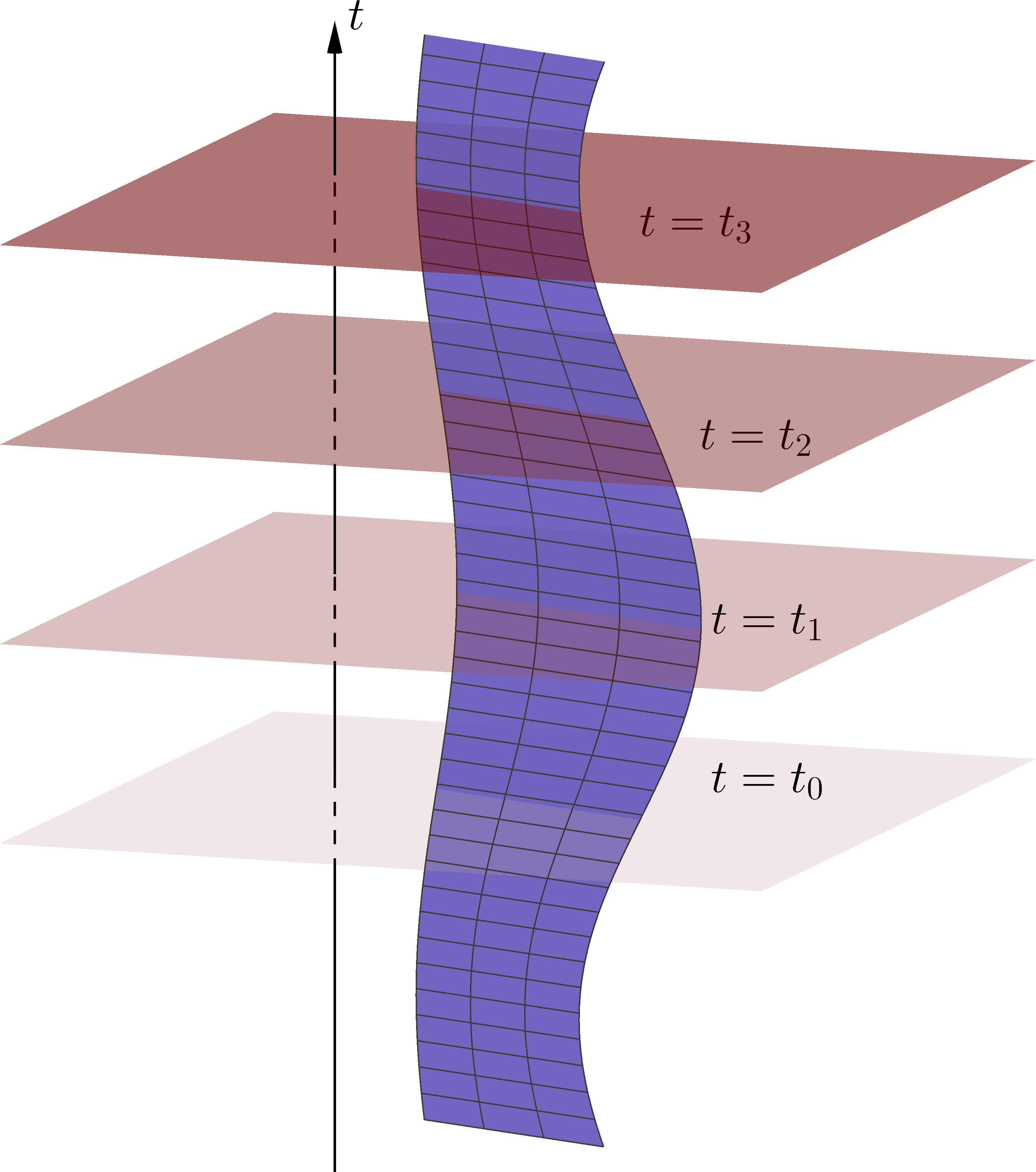
Figure 1: Graphical depiction of the embedding of timelike Newton–Cartan submanifolds. The vertical direction represents the time $t$, while the spatial directions are in the plane orthogonal to the $t$–axis. The spatial hypersurfaces of constant time are denoted by their corresponding value of $t$. Note in particular that the condition (2.24) implies that the submanifold does not “bend” away from the time direction in the ambient spacetime.

The description of submanifolds in NC geometry must be invariant under Galilean boosts, as these just express a choice of frame. This implies that the defining structure of NC submanifolds, namely (2.17) and (2.20), must be invariant under local Galilean boost transformations. We start by noting that the embedding map does not transform under boosts, that is

$$\delta_{G}X^{\mu}=0~{}~{}\Rightarrow~{}~{}\delta_{G}u^{\mu}_{a}=0~{}~{},$$ (2.30)

and hence the tangent vectors to the surface are boost-invariant. Specialising to timelike submanifolds, using (2.25), the variations of (2.17) and (2.20), together with (2.30), require

$$\begin{split}u^{\mu}_{a}\delta_{G}n_{\mu}^{I}=&-n_{\mu}^{I}\delta_{G}u^{\mu}_{a}~{}~{},~{}~{}n^{\mu J}\delta_{G}n_{\mu}^{I}=0~{}~{}\Rightarrow~{}~{}\delta_{G}n_{\mu}^{I}=0~{}~{},\\ u_{\mu}^{a}h^{\mu\nu}\delta_{G}n_{\mu I}=&-n^{\mu}_{I}\delta_{G}u_{\mu}^{a}~{}~{},~{}~{}u^{\mu}_{a}\delta_{G}u^{b}_{\mu}=-u_{\mu}^{b}\delta_{G}u^{\mu}_{a}~{}~{}\Rightarrow~{}~{}\delta_{G}u^{a}_{\mu}=0~{}~{},\end{split}$$ (2.31)

while $\delta_{G}n^{\mu}_{I}=0$ follows trivially from (2.25). Thus, Eq. (2.30) ensures that the defining structure of timelike NC submanifolds is boost-invariant.

2.2.3 Induced Newton–Cartan structures

Besides the defining conditions (2.17) and (2.20), NC submanifolds have other inherent geometric structures, such as induced tensors, that can be introduced via appropriate contractions of ambient tensors with any of the objects $u_{\mu}^{a}$ and $u^{\mu}_{a}$. We wish to identify the induced NC structures on the submanifold that have the same properties as the NC structures of the ambient spacetime. For instance, these induced structures should transform as in (2.4) and (2.5) but now involving only tangential directions to the submanifold.

The basic building blocks are the clock 1-form $\tau_{a}$ in eq. (2.23) and the normal velocity $v^{I}$ in eq. (2.29) along with the pullbacks of the remaining ambient space fields

$$h_{ab}=u^{\mu}_{a}u^{\nu}_{b}h_{\mu\nu}\,,\qquad v^{a}=u^{a}_{\mu}v^{\mu}\,,\qquad h^{ab}=u^{a}_{\mu}u^{b}_{\nu}h^{\mu\nu}\,,\qquad m_{a}=u^{\mu}_{a}m_{\mu}~{}~{}.$$ (2.32)

It is possible to see that these structures mimic many of the properties of the ambient NC structure. For instance we have $\tau_{a}h^{ab}=0$ and $v^{a}\tau_{a}=-1$ by virtue of (2.24) and $\tau_{\mu}h^{\mu\nu}=0$ as well as $v^{\mu}\tau_{\mu}=-1$. Additionally, they give rise to the completeness relation $h^{ac}h_{cb}=\delta^{a}_{b}+v^{a}\tau_{b}$, which in turn implies the relation $h^{\mu\nu}u_{\mu}^{a}=h^{ab}u_{b}^{\nu}$. However, using (2.29), we find that

$$v^{a}h_{ab}=u^{a}_{\mu}v^{\mu}u^{\rho}_{a}u^{\sigma}_{b}h_{\rho\sigma}=-v^{I}h_{Ib}=-v^{I}v^{I}\tau_{b}~{}~{},$$ (2.33)

which is non-zero, contrary to the corresponding ambient NC result $v^{\mu}h_{\mu\nu}=0$. Hence, the individual structures in (2.32) do not form a NC geometry on the submanifold. Using (2.33) we instead define

$${\check{h}_{ab}=h_{ab}-v^{I}v_{I}\tau_{a}\tau_{b}~{}~{},}$$ (2.34)

which leads to a completeness relation and satisfies the required orthogonality condition, that is

$$h^{ac}\check{h}_{cb}=\delta^{a}_{b}+\tau_{b}v^{a}~{}~{},~{}~{}v^{a}\check{h}_{ab}=0~{}~{}.$$ (2.35)

For $\check{h}_{ab}$ to be considered a NC structure on the submanifold, one must also ensure that it transforms under Galilean boosts as its ambient space counterpart $h_{\mu\nu}$ (cf. (2.5)). Using (2.4), (2.5), (2.31) and $v^{a}\lambda_{a}=-v^{I}\lambda_{I}$, it can be shown that

$$\begin{split}\delta_{G}v^{a}&=h^{ab}\check{\lambda}_{b}~{}~{},~{}~{}\delta_{G}(v^{a}h_{ab})=-2\tau_{b}\lambda^{I}v_{I}~{}~{},~{}~{}\delta_{G}h_{ab}=2\tau_{(a}\lambda_{b)}~{}~{},\\ \delta_{G}\check{h}_{ab}&=2\tau_{(a}\lambda_{b)}-2\tau_{a}\tau_{b}v^{I}\lambda_{I}=2\tau_{(a}\lambda_{b)}+2\tau_{a}\tau_{b}v^{c}\lambda_{c}=2\tau_{(a}\check{\lambda}_{b)}~{}~{},\end{split}$$ (2.36)

where we have defined

$$\check{\lambda}_{a}=\lambda_{a}+v^{c}\lambda_{c}\tau_{a}=\check{h}_{ab}h^{bc}\lambda_{c}~{}~{},$$ (2.37)

which satisfies $v^{a}\check{\lambda}_{a}=0$, analogously to the ambient orthogonality condition $v^{\mu}\lambda_{\mu}=0$. Thus $\check{h}_{ab}$ transforms under submanifold Galilean boosts in the same manner as $h_{\mu\nu}$ transforms under ambient Galilean boosts.

NC submanifolds admit boost-invariant structures similar to the ambient structures (2.6) and (2.8). Given that the set of tangent and normal vectors is boost-invariant (see eq. (2.31)), two of these structures are obtained by contractions of the corresponding ambient quantities, namely

$$\bar{h}_{ab}=u^{\mu}_{a}u^{\nu}_{b}\bar{h}_{\mu\nu}=\check{h}_{ab}-2\tau_{(a}\check{m}_{b)}~{}~{},~{}~{}\hat{v}^{a}=u_{\mu}^{a}\hat{v}^{\mu}=v^{a}-h^{ab}\check{m}_{b}~{}~{},$$ (2.38)

where we have defined the submanifold $U(1)$ connection

$${\check{m}_{a}=m_{a}-\frac{1}{2}v^{I}v_{I}\tau_{a}\,,}$$ (2.39)

which transforms under boosts as $\delta_{G}\check{m}_{a}=\check{\lambda}_{a}$, analogous to the boost transformation of the ambient connection $m_{\mu}$. Given that in the ambient space we have the identity $\hat{v}^{\nu}\bar{h}_{\nu\mu}=2\tilde{\Phi}\tau_{\mu}$ where $\tilde{\Phi}$ is defined in (2.8) we require an analogue condition of the form $\hat{v}^{a}\bar{h}_{ab}=2\check{\Phi}\tau_{b}$ for some scalar $\check{\Phi}$. Explicit manipulation shows that

$$\hat{v}^{a}\bar{h}_{ab}=u^{a}_{\mu}\hat{v}^{\mu}u^{\nu}_{a}u^{\rho}_{b}\bar{h}_{\nu\rho}=\hat{v}^{\nu}\bar{h}_{\nu\rho}u^{\rho}_{b}-n^{I}_{\mu}h^{\nu\sigma}n^{I}_{\sigma}\hat{v}^{\mu}u^{\rho}_{b}\bar{h}_{\nu\rho}=2(\tilde{\Phi}-1/2\hat{v}^{I}\hat{v}^{I})\tau_{b}~{}~{},$$ (2.40)

which leads us to identify

$$\check{\Phi}=\tilde{\Phi}-\frac{1}{2}\hat{v}^{I}\hat{v}^{I}=-v^{a}\check{m}_{a}+\frac{1}{2}h^{ab}\check{m}_{a}\check{m}_{b}~{}~{},$$ (2.41)

thus taking the same form as its ambient counterpart (2.8) but now in terms of $\check{m}_{a}$.

In summary, we define the induced Newton–Cartan structure on the submanifold $\Sigma_{p+1}$ to consist of the fields $(\tau_{a},\check{h}_{ab},\check{m}_{a})$ and $(v^{a},h^{ab})$ along with the boost invariant combinations $\hat{v}^{a}$, $\bar{h}_{ab}$ and $\check{\Phi}$, satisfying the relations

$$\delta^{a}_{b}=h^{ac}\check{h}_{cb}-\tau_{b}v^{a}~{}~{},~{}~{}\tau_{a}h^{ab}=0\,,\qquad v^{a}\check{h}_{ab}=0~{}~{},$$ (2.42)

as well as

$$\hat{v}^{a}\bar{h}_{ab}=2\check{\Phi}\tau_{b}~{}~{}.$$ (2.43)

These are related to the ambient Newton–Cartan structures in the following way

$$\tau_{a}=u^{\mu}_{a}\tau_{\mu}\,,\qquad\check{h}_{ab}=u^{\mu}_{a}u^{\nu}_{b}h_{\mu\nu}-v^{I}v_{I}\tau_{a}\tau_{b}=h_{ab}-v^{I}v_{I}\tau_{a}\tau_{b}~{}~{},$$ (2.44)

$$\check{m}_{a}=u^{\mu}_{a}m_{\mu}-\frac{1}{2}v^{I}v_{I}\tau_{a}=m_{a}-\frac{1}{2}v^{I}v_{I}\tau_{a}\,,\qquad v^{a}=u^{a}_{\mu}v^{\mu},\qquad h^{ab}=u^{a}_{\mu}u^{b}_{\nu}h^{\mu\nu}~{}~{},$$ (2.45)

$$\hat{v}^{a}=v^{a}-h^{ab}\check{m}_{b}=u^{a}_{\mu}\hat{v}^{\mu}\,,\qquad\bar{h}_{ab}=\check{h}_{ab}-2\tau_{(a}\check{m}_{b)}=u^{\mu}_{a}u^{\nu}_{b}\bar{h}_{\mu\nu}~{}~{},$$ (2.46)

$$\check{\Phi}=-v^{a}\check{m}_{a}+\frac{1}{2}h^{ab}\check{m}_{a}\check{m}_{b}=\tilde{\Phi}-\frac{1}{2}\hat{v}^{I}\hat{v}^{I}~{}~{}.$$ (2.47)

These structures transform according to

$$\delta\tau_{a}=\pounds_{\zeta}\tau_{a}~{}~{},~{}~{}\delta\check{h}_{ab}=\pounds_{\zeta}\check{h}_{ab}+2\check{\lambda}_{(a}\tau_{b)}~{}~{},~{}~{}\delta\check{m}_{a}=\pounds_{\zeta}\check{m}_{a}+\check{\lambda}_{a}+{\partial}_{a}\sigma~{}~{},$$ (2.48)

$$\delta v^{a}=\pounds_{\zeta}v^{a}+h^{ab}\check{\lambda}_{b}~{}~{},~{}~{}\delta h^{ab}=\pounds_{\zeta}h^{ab}~{}~{},$$ (2.49)

$$\delta\hat{v}^{a}=\pounds_{\zeta}\hat{v}^{a}-h^{ab}{\partial}_{b}\sigma~{}~{},~{}~{}\delta\bar{h}_{ab}=\pounds_{\zeta}\bar{h}_{ab}-2\tau_{(a}{\partial}_{b)}\sigma~{}~{},~{}~{}\delta\check{\Phi}=\pounds_{\zeta}\check{\Phi}-\hat{v}^{a}{\partial}_{a}\sigma~{},$$ (2.50)

under submanifold diffeomorphisms $\zeta^{a}$, Galilean boosts $\check{\lambda}_{a}$ (satisfying $v^{a}\check{\lambda}_{a}=0$) and $U(1)$ gauge transformations $\sigma$.

2.2.4 The role of the transverse velocity $v^{I}$

In order to elucidate the role of $v^{I}$, we consider for concreteness a co-dimension one submanifold $\Sigma$ moving with (constant) linear velocity $v^{\mu}_{\Sigma}=(0,0,0,\mathfrak{v})$ in the $z$-direction of a four-dimensional flat ambient Newton–Cartan spacetime, which was introduced in (2.15) and where $i$ runs only over spatial directions. Defining $\Sigma$ via the embedding equation

$$F(x,y,z-\mathfrak{v}t)=0~{}~{},$$ (2.51)

we can write the normal 1-form as

$$n=N\text{d}F=N{\partial}_{x}F+N{\partial}_{y}F+N{\partial}_{u}F\text{d}z-\mathfrak{v}{\partial}_{u}F\text{d}t~{}~{},$$ (2.52)

where we have defined $u=z-\mathfrak{v}t$ and where $N$ is fixed by the normalisation condition (2.17). This means that

$$v^{\mu}n_{\mu}=-n_{0}=\mathfrak{v}N{\partial}_{u}F,~{}~{},~{}~{}v^{\mu}_{\Sigma}n_{\mu}=\mathfrak{v}n_{z}=\mathfrak{v}N{\partial}_{u}F~{}~{},$$ (2.53)

leading us to conclude that $v^{\mu}n_{\mu}=v^{\mu}_{\Sigma}n_{\mu}$. Thus, the normal projection of the NC velocity is the same as the normal projection of the linear velocity vector $v^{\mu}_{\Sigma}$ of the submanifold $\Sigma$.

To illustrate this in the simplest possible setting, we consider an infinitely extended moving flat membrane embedded in $(3+1)$-dimensional flat NC space, described by

$$u=z-\mathfrak{v}t=0~{}~{},$$ (2.54)

leading to the normal 1-form

$$n_{\mu}=-\mathfrak{v}\delta^{0}_{\mu}+\delta^{3}_{\mu}~{}~{}\Rightarrow~{}~{}v^{\mu}n_{\mu}=\mathfrak{v}~{}~{}.$$ (2.55)

Therefore, for a flat brane, where the normal vector is the same everywhere, we see that the normal projection of the NC velocity vector is just the magnitude of the linear velocity of the plane.

2.2.5 Covariant derivatives, extrinsic curvature and external rotation

Since we are dealing with the description of a single surface, and not of a foliation, covariant differentiation of submanifold structures only has meaning along tangential directions to the surface. Analogously to Lorentzian surfaces (see e.g. Armas and Tarrio (2018)), we define a covariant derivative along surface directions that is compatible both with the surface Newton–Cartan structure, $D_{a}\tau_{b}=0=D_{a}h^{bc}$, and the ambient Newton–Cartan structure, $D_{a}\tau_{\mu}=0=D_{a}h^{\mu\nu}$, that acts on an arbitrary mixed tensor $T^{b\mu}$ as

$${D_{a}T^{b\mu}={\partial}_{a}T^{b\mu}+\gamma^{b}_{ac}T^{c\mu}+u^{\rho}_{a}\Gamma^{\mu}_{\rho\lambda}T^{b\lambda}~{}~{},}$$ (2.56)

where we have introduced the surface affine connection according to

$${\gamma}^{c}_{ab}=-\hat{v}^{c}{\partial}_{a}\tau_{b}+\frac{1}{2}h^{cd}\left({\partial}_{a}\bar{h}_{bd}+{\partial}_{b}\bar{h}_{ad}-{\partial}_{d}\bar{h}_{ab}\right)~{}~{},$$ (2.57)

in analogy with the the spacetime affine connection (2.10). Note in particular that $D_{a}$ does not act on transverse indices. The relation between ${\gamma}^{c}_{ab}$ and $\Gamma^{\mu}_{\rho\lambda}$ is obtained in appendix C and is shown to be

$$\gamma^{c}_{ab}=\Gamma^{c}_{ab}+u^{c}_{\mu}{\partial}_{a}u^{\mu}_{b}=u^{c}_{\mu}u^{\nu}_{a}\nabla_{\nu}u^{\mu}_{b}~{}~{},$$ (2.58)

where the corresponding surface torsion tensor is

$$2\gamma^{c}_{[ab]}=-\hat{v}^{c}\tau_{ab}=-\hat{v}^{c}u^{\mu}_{a}u^{\nu}_{b}\tau_{\mu\nu}~{}~{},$$ (2.59)

and where the last equality follows from the fact that exterior derivatives commute with pullbacks.

It is also convenient to introduce a covariant derivative ${\mathfrak{D}}_{a}$ that acts on all indices, i.e. $\mu,a,I$ Armas and Tarrio (2018), and whose action on the normal 1-forms and tangent vectors allows for the Weingarten decomposition

$$\begin{split}{\mathfrak{D}}_{a}n^{I}_{\sigma}&={\partial}_{a}n^{I}_{\sigma}-\Gamma^{\lambda}_{\mu\sigma}u^{\mu}_{a}n_{\lambda}^{I}-\omega_{a}{{}^{I}}{{}_{J}}n_{\sigma}^{J}=-u^{b}_{\sigma}K_{ab}{{}^{I}}+\frac{1}{2}u^{b}_{\sigma}\hat{v}^{I}\tau_{ab}~{}~{},\\ {\mathfrak{D}}_{a}u_{b}^{\mu}&=D_{a}u_{b}^{\mu}=n^{\mu}_{I}K_{ab}{{}^{I}}-\frac{1}{2}n^{\mu}_{I}\hat{v}^{I}\tau_{ab}~{}~{},\end{split}$$ (2.60)

where we have defined the extrinsic curvature to the submanifold according to

$$K_{ab}{{}^{I}}=n_{\mu}^{I}D_{a}u^{\mu}_{b}+\frac{1}{2}\hat{v}^{I}\tau_{ab}=n_{\mu}^{I}\left(\partial_{a}u^{\mu}_{b}+u^{\nu}_{a}u^{\rho}_{b}\Gamma_{(\nu\rho)}^{\mu}\right)=-u^{\mu}_{a}u^{\nu}_{b}\nabla_{(\mu}n_{\nu)}^{I}~{}~{}.$$ (2.61)

The extrinsic curvature tensor, when defined in this manner, is symmetric and invariant under Galilean boosts but transforms under $U(1)$ gauge transformations according to

$$\delta_{\sigma}K_{ab}{}^{I}=\frac{1}{2}\tau_{Ia}\partial_{b}\sigma+\frac{1}{2}\tau_{Ib}\partial_{a}\sigma\,,$$ (2.62)

where we used (2.14). In (2.60) we also introduced the external rotation tensor, which can be interpreted as a $SO(d-p)$ connection, defined as

$$\omega_{a}{{}^{I}}{{}_{J}}=n^{\mu}_{J}D_{a}n^{I}_{\mu}~{}~{},$$ (2.63)

which is antisymmetric in $I,J$ indices and transforms under $U(1)$ gauge transformations as

$$\delta_{\sigma}\omega_{a}{{}^{I}}{{}_{J}}=-\frac{1}{2}\left(\tau_{aJ}\partial^{I}\sigma+{\tau^{I}}_{J}\partial_{a}\sigma+{\tau^{I}}_{a}\partial_{J}\sigma\right)~{}~{}.$$ (2.64)

If the submanifold is co-dimension one, the external rotation vanishes by definition.

Both the extrinsic curvature tensor and the external rotation tensor introduced here are direct analogues of their Lorentzian counterparts Armas and Tarrio (2018). To see that $\omega_{a}{{}^{I}}{{}_{J}}$ transforms as a connection we examine what happens if we perform a local $SO(d-p)$ rotation of the normal vectors as in (2.18). If we focus on an infinitesimal rotation ${\mathcal{M}^{I}}_{J}=\delta^{I}_{J}+\lambda^{I}{}_{J}$ where $\lambda^{I}{}_{J}=-\lambda^{J}{}_{I}$, the extrinsic curvature tensor and external rotation tensor transform as

$$\delta_{\lambda}K_{ab}{{}^{I}}=\lambda^{I}{{}_{J}}K_{ab}{{}^{J}}~{}~{},~{}~{}\delta_{\lambda}\omega_{a}{{}^{I}}{{}_{J}}=\partial_{a}\lambda^{I}{}_{J}+\lambda^{I}{{}_{K}}\omega_{a}{{}^{K}}{{}_{J}}+\lambda_{J}{{}^{K}}\omega_{a}{{}^{I}}{{}_{K}}~{}~{}.$$ (2.65)

In addition, under a change of sign of the normal vectors $n^{\mu}_{I}\to-n^{\mu}_{I}$, the extrinsic curvature changes sign.

2.2.6 Integrability conditions

Certain combinations of geometric structures of Lorentzian submanifolds are related to specific contractions of the Riemann tensor of the ambient space. These are known as integrability conditions. In this section we derive the analogous conditions in the context of NC submanifolds, which are known as the Codazzi–Mainardi, Gauss–Codazzi and Ricci–Voss equations. In order to do so, we note that in the presence of torsion, the Ricci identity takes the form

$$[\nabla_{\mu},\nabla_{\nu}]X_{\sigma}=R_{\mu\nu\sigma}{{}^{\rho}}X_{\rho}-2\Gamma^{\rho}_{[\mu\nu]}\nabla_{\rho}X_{\sigma}~{}~{},$$ (2.66)

where the Riemann tensor $R_{\mu\nu\sigma}{{}^{\rho}}$ of the ambient space is given by

$$R_{\mu\nu\sigma}{{}^{\rho}}=-{\partial}_{\mu}\Gamma^{\rho}_{\nu\sigma}+{\partial}_{\nu}\Gamma^{\rho}_{\mu\sigma}-\Gamma^{\rho}_{\mu\lambda}\Gamma^{\lambda}_{\nu\sigma}+\Gamma^{\rho}_{\nu\lambda}\Gamma^{\lambda}_{\mu\sigma}~{}~{}.$$ (2.67)

The integrability conditions to be derived below take a nice form if we work with an object that is closely related to the extrinsic curvature, namely

$$\tilde{K}_{ab}{{}^{I}}=n_{\mu}^{I}D_{a}u^{\mu}_{b}=K_{ab}{{}^{I}}-\frac{1}{2}\hat{v}^{I}\tau_{ab}~{}~{},$$ (2.68)

which has a non-vanishing antisymmetric part $2\tilde{K}_{[ab]}{{}^{J}}=-\hat{v}^{J}\tau_{ab}$.

We begin by deriving the Codazzi–Mainardi equation (see e.g. Armas and Tarrio (2018); Aminov (2014)) by considering the quantity $D_{a}\tilde{K}_{bc}{{}^{I}}-D_{b}\tilde{K}_{ac}{{}^{I}}$. We find

$$D_{a}\tilde{K}_{bc}{{}^{I}}=\tilde{K}_{ab}{{}^{I}}n_{I}^{\rho}(\nabla_{\rho}u^{\mu}_{c})n^{I}_{\mu}-\omega_{b}{{}^{I}}{{}_{J}}\tilde{K}_{ac}{{}^{J}}-u^{\mu}_{c}u^{\rho}_{a}u^{\sigma}_{b} \nabla_{\rho}\nabla_{\sigma}n_{\mu}^{I}~{}~{},$$ (2.69)

where we used (2.63). From here, using (2.66) and the covariant derivative ${\mathfrak{D}}_{a}$ introduced in (2.60) we derive the Codazzi–Mainardi equation

$${\mathfrak{D}}_{a}\tilde{K}_{bc}{{}^{I}}-{\mathfrak{D}}_{b}\tilde{K}_{ac}{{}^{I}}=-R_{abc}{{}^{I}}+\hat{v}^{d}\tau_{ab}\tilde{K}_{dc}{{}^{I}}~{}~{}.$$ (2.70)

In order to derive the Gauss–Codazzi equation, we let $\omega_{c}$ be any submanifold 1-form that is the pullback of $\omega_{\mu}$ whose normal components vanish, i.e. $\omega_{\mu}=u^{c}_{\mu}\omega_{c}$. The Ricci identity for the submanifold reads

$$[D_{a},D_{b}]\omega_{c}={\mathcal{R}}_{abc}{{}^{d}}\omega_{d}+\hat{v}^{d}\tau_{ab}D_{d}\omega_{c}~{}~{},$$ (2.71)

where ${\mathcal{R}}_{abc}{{}^{d}}$ is the Riemann tensor of the submanifold and takes the same form as (2.67) but with the connection $\Gamma^{\rho}_{\nu\sigma}$ replaced by $\gamma^{c}_{ab}$ of (2.57). Using $u_{\mu}^{a}D_{b}u_{c}^{\mu}=0$ (which follows from (2.58)) and $n^{\mu}_{I}D_{b}u_{\mu}^{d}=h^{de}\tilde{K}_{beI}$, explicit manipulation leads to

$${\mathcal{R}}_{abc}{{}^{d}}\omega_{d}+\hat{v}^{d}\tau_{ab}D_{d}\omega_{c}= h^{ed}\tilde{K}_{ac}{{}^{I}}\tilde{K}_{beI}\omega_{d}-h^{ed}\tilde{K}_{bc}{{}^{I}}\tilde{K}_{aeI}\omega_{d}+R_{abc}{{}^{d}}\omega_{d}$$

$$+\tau_{ab}\left(-\hat{v}^{I}n^{\rho}_{I}u^{\mu}_{c}\nabla_{\rho}\omega_{\mu}+\hat{v}^{\nu}u^{\mu}_{c}\nabla_{\nu}\omega_{\mu}\right)~{}~{},$$ (2.72)

where we used (2.66). In this expression, the terms proportional to $\tau_{ab}$ on both sides cancel and since it must be true for any one form $\omega_{c}$, the Gauss–Codazzi equation becomes

$${{\mathcal{R}}_{abc}{{}^{d}}=\tilde{K}_{ac}{{}^{I}}\tilde{K}_{b}{{}^{d}}{{}_{I}}-\tilde{K}_{bc}{{}^{I}}\tilde{K}_{a}{{}^{d}}{{}_{I}}+R_{abc}{{}^{d}}\,,}$$ (2.73)

where $\tilde{K}_{b}{{}^{d}}{{}_{I}}=h^{dc}\tilde{K}_{bc}{{}_{I}}$.

Although we will not use it in this paper, we will briefly discuss the Ricci–Voss equation for completeness. This equation becomes useful for surfaces of co-dimension higher than one, where we can define the outer curvature in terms of the external rotation tensor (2.63) as

$$\Omega^{I}{{}_{Jab}=2{\partial}_{[a}\omega_{b]}{{}^{I}}{{}_{J}}-2\omega_{[a|}{{}^{I}}{}_{K}\omega_{|b]}{}^{K}{}_{J}~{}~{}.}$$ (2.74)

In terms of this tensor, the Ricci–Voss equation for Newton–Cartan geometry can be shown to read

$$\Omega^{I}{}_{Jab}=R_{abJ}{{}^{I}}-2h^{cd}\tilde{K}_{[a|c}{{}^{I}}\tilde{K}_{|b]dJ}~{}~{}.$$ (2.75)

This completes the description of the geometric structures of NC submanifolds.

3 Variations and dynamics of Newton–Cartan submanifolds

In the previous section we defined timelike NC submanifolds and their characteristic geometric properties. In this section, closely following the Lorentzian case Armas and Tarrio (2018), we develop the variational calculus for NC submanifolds for the geometric structures of interest. These results are necessary to later introduce geometric action functionals capable of describing different types of soft matter systems, including the case of bending energies for lipid vesicles.

3.1 Variations of Newton–Cartan objects on the submanifold

In the following, we consider two types of variations, namely embedding map variations, which are displacements of the submanifold, and Lagrangian variations which consist of the class of diffeomorphisms that displace the ambient space but keep the embedding map fixed (see e.g. Carter (1993, 1997) and also Armas (2013); Armas and Tarrio (2018)). As in the Lorentzian case Armas and Tarrio (2018), the sum of these two types of variations yield the transformation properties of the submanifold structures under full ambient space diffeomorphisms. When considering action functionals that give dynamics to submanifolds, they are equivalent, up to normal rotations.

3.1.1 Embedding map variations

Before specialising to any of the two types of variations, it is useful to consider general variations of the normal vectors. In particular, we decompose the variation of the normal vectors as

$$\delta n_{\mu}^{I}=u^{a}_{\mu}u^{\nu}_{a}\delta n^{I}_{\nu}+n^{J}_{\mu}n^{\nu}_{J}\delta n^{I}_{\nu}=-u^{a}_{\mu}n^{I}_{\nu}\delta u^{\nu}_{a}+\frac{1}{2}n_{\mu J}(n^{\nu J}\delta n^{I}_{\nu}+n^{\nu I}\delta n^{J}_{\nu})+\lambda^{I}{}_{J}n_{\mu}^{J}~{}~{},$$ (3.76)

where

$$\lambda^{I}{}_{J}=\frac{1}{2}\left(n^{\nu}_{J}\delta n^{I}_{\nu}-n^{\nu I}\delta n_{J\nu}\right)~{}~{},$$ (3.77)

is a local $\mathfrak{so}(d-p)$ transformation of the normal vectors. By varying the second relation in (2.17), we find the relation $n^{\nu J}\delta n^{I}_{\nu}+n^{\nu I}\delta n^{J}_{\nu}=-n_{\mu}^{I}n_{\nu}^{J}\delta h^{\mu\nu}$ and hence

$$\delta n_{\mu}^{I}=-u^{a}_{\mu}n^{I}_{\nu}\delta u^{\nu}_{a}-\frac{1}{2}n_{\mu J}n_{\nu}^{I}n_{\rho}^{J}\delta h^{\nu\rho}+\lambda^{I}{}_{J}n_{\mu}^{J}~{}~{}.$$ (3.78)

By varying the completeness relation (2.19) one may express variations of $\delta h^{\nu\rho}$ in terms of variations of $\tau_{\nu}$ and $h_{\nu\rho}$ such that $\delta h^{\mu\nu}=2v^{(\mu}h^{\nu)\lambda}\delta\tau_{\lambda}-h^{\mu\rho}h^{\nu\sigma}\delta h_{\rho\sigma}$. This leads to

$${\delta n_{\mu}^{I}=-v^{(I}n^{J)\nu}n_{\mu J}\delta\tau_{\nu}+\frac{1}{2}n^{\rho J}n_{\mu J}n^{\nu I}\delta h_{\rho\nu}-{n}^{I}_{\nu}u^{a}_{\mu}\delta u^{\nu}_{a}+\lambda^{I}{}_{J}n_{\mu}^{J}~{}~{},}$$ (3.79)

which describes arbitrary infinitesimal variations of the normal vectors.

We now specialise to infinitesimal variations of the embedding map which we denote by

$$\delta X^{\mu}(\sigma)=-\xi^{\mu}(\sigma)~{}~{},$$ (3.80)

where $\xi^{\mu}(\sigma)$ is understood as being an infinitesimal first order variation. Under this variation, the ambient tensor structures evaluated at the surface (i.e. $\tau_{\mu}(X)$, $\bar{h}_{\mu\nu}(X)$) vary as

$$\delta_{X}\tau_{\mu}(X)=-\xi^{\nu}{\partial}_{\nu}\tau_{\mu}~{}~{},~{}~{}\delta_{X}\bar{h}_{\mu\nu}(X)=-\xi^{\rho}{\partial}_{\rho}\bar{h}_{\mu\nu}~{}~{},$$ (3.81)

which follows from $\delta_{X}\tau_{\mu}(X)=\tau_{\mu}(X-\xi)-\tau_{\mu}(X)=-\xi^{\nu}{\partial}_{\nu}\tau_{\mu}+\mathcal{O}(\xi^{2})$. In turn, the tangent vectors transform as

$$\delta_{X}u^{\mu}_{a}={\partial}_{a}\delta X^{\mu}=-{\partial}_{a}\xi^{\mu}~{}~{},$$ (3.82)

while variations of the induced metric structures take the form

$$\delta_{X}\tau_{a}=-u^{\mu}_{a}\pounds_{\xi}\tau_{\mu},\qquad\delta_{X}\bar{h}_{ab}=-u^{\mu}_{a}u^{\nu}_{b}\pounds_{\xi}\bar{h}_{\mu\nu}~{}~{}.$$ (3.83)

In other words, for these structures, performing embedding map variations is equivalent to performing a diffeomorphism in the space of embedding maps that keep $u^{\mu}_{a}$ fixed, i.e. they are diffeomorphisms that are independent of $\sigma^{a}$. Using (3.79), we can write the variation of the normal vector as

$$\delta_{X}n_{\mu}^{I}=-n_{\mu J}n_{\rho}^{(I}n^{J)\nu}\nabla_{\nu}\xi^{\rho}-n_{\mu J}\hat{v}^{(I}n^{J)\nu}\tau_{\nu\rho}\xi^{\rho}+n^{I}_{\rho}{\partial}_{\mu}\xi^{\rho}+\widetilde{\lambda}^{IJ}n_{\mu J}~{}~{},$$ (3.84)

where the third term ensures that the orthogonality relation $u^{\mu}_{a}n^{I}_{\mu}=0$ is obeyed after the variation while the last term is a local transverse rotation of the form $\widetilde{\lambda}^{IJ}=\lambda^{IJ}+n_{\rho}^{[J}n^{I]\nu}{\partial}_{\nu}\xi^{\rho}$.

For the purposes of this work, as mentioned in sec. 2.1.3, we will be focusing on ambient NC geometries with absolute time, i.e. zero torsion. This extra assumption greatly simplifies many expressions after variation. We stress, however, that it is in general not possible to assume zero torsion before variation, as variation and setting torsion to zero do not always commute.

However, specifically in the case of embedding map or Lagrangian variations, the variation of $\tau_{\mu\nu}$ is guaranteed to vanish when the torsion itself vanishes. This means that we can set torsion to zero in the Lagrangian if all we are interested in are the equations of motion for $X^{\mu}$. For example $\delta_{X}\tau_{\mu\nu}(X)=-\xi^{\rho}\partial_{\rho}\tau_{\mu\nu}$, which vanishes when $\text{d}\tau=0$. Under the assumption of vanishing torsion, variations of the extrinsic curvature (2.61) take the form

$$\delta_{X}K_{ab}{{}^{I}} = (\delta_{X}n^{I}_{\mu}){\partial}_{a}u^{\mu}_{b}-n^{I}_{\mu}{\partial}_{a}{\partial}_{b}\xi^{\mu}+(\delta_{X}n^{I}_{\mu})u^{\rho}_{a}\Gamma^{\mu}_{\rho\lambda}u^{\lambda}_{b}$$ (3.85)

$$-n^{I}_{\mu}({\partial}_{a}\xi^{\rho})\Gamma^{\mu}_{\rho\lambda}u^{\lambda}_{b}-n^{I}_{\mu}u^{\rho}_{a}\xi^{\kappa}{\partial}_{\kappa}(\Gamma^{\mu}_{\rho\lambda})u^{\lambda}_{b}-n^{I}_{\mu}u^{\rho}_{a}\Gamma^{\mu}_{\rho\lambda}{\partial}_{b}\xi^{\lambda}$$

$$= -n_{\mu}^{I}D_{a}D_{b}\xi^{\mu}+\xi^{\rho}R_{\rho ab}{{}^{I}}+n_{\rho}^{[I}n^{J]\nu}\Gamma^{\rho}_{\nu\sigma}\xi^{\sigma}K_{abJ}~{}~{},$$

where we have used (3.84) as well as $\delta_{X}\Gamma^{\mu}_{\rho\lambda}(X)=-\xi^{\kappa}{\partial}_{\kappa}\Gamma^{\mu}_{\rho\lambda}$. The last term in (3.85) denotes a local $\mathfrak{so}(d-p)$ transformation and we have explicitly ignored further rotations by setting $\lambda^{IJ}=0$ in (3.79). It is also straightforward to consider variations of the external rotation tensor (2.63) but since we do not explicitly consider this structure in the dynamics of submanifolds, we will not dwell on this.

3.1.2 Lagrangian variations

In the previous section we have described how to perform variations of the embedding map. In this section we focus on a particular class of diffeomorphisms $x^{\mu}\to x^{\mu}-\xi^{\mu}$ that only act on fields with support in the entire ambient spacetime, that is, they only act on the NC triplet $(\tau_{\mu}(x),h_{\mu\nu}(x),m_{\mu}(x))$. In general, diffeomorphisms also displace the embedding map according to $\delta_{\xi}X^{\mu}=-\xi^{\mu}$ where $\delta_{\xi}$ denotes an infinitesimal diffeomorphism variation. However, here we consider the case of Lagrangian variations for which $\delta_{\xi}X^{\mu}=0$ (see e.g. Carter (1993, 1997); Armas (2013); Armas and Tarrio (2018)). In turn, this implies that the tangent vectors do not vary, that is

$$\delta_{\xi}u^{\mu}_{a}=0~{}~{}.$$ (3.86)

In the remainder of this section, we will explicitly work out Lagrangian variations of submanifold structures and compare them with embedding map variations, thereby extracting the transformation properties under full ambient diffeomorphisms. In particular, using (3.86) and the fact that $\delta_{\xi}\tau_{\mu}=\pounds_{\xi}\tau_{\mu}$ and $\delta_{\xi}\bar{h}_{\mu\nu}=\pounds_{\xi}\bar{h}_{\mu\nu}$ we find

$$\delta_{\xi}\tau_{a}=u^{\mu}_{a}\pounds_{\xi}\tau_{\mu}~{}~{},~{}~{}\delta_{\xi}\bar{h}_{ab}=u^{\mu}_{a}u^{\nu}_{b}\pounds_{\xi}\bar{h}_{\mu\nu}~{}~{}.$$ (3.87)

Comparing this with (3.83), it follows that for pullbacks of Newton–Cartan objects we have the relations

$$(\delta_{\xi}+\delta_{X})\tau_{a}=(\delta_{\xi}+\delta_{X})\bar{h}_{ab}=0~{}~{},$$ (3.88)

and thus these objects transform as scalars under ambient diffeomorphisms. For later purposes, we rewrite these results as

$$\delta_{\xi}\tau_{a} = \tau_{\rho}D_{a}\xi^{\rho}~{}~{},$$ (3.89)

$$\delta_{\xi}\bar{h}_{ab} = \bar{h}_{\rho b}D_{a}\xi^{\rho}+\bar{h}_{\rho a}D_{b}\xi^{\rho}-2\tau_{a}\tau_{b}\xi^{\sigma}{\partial}_{\sigma}\tilde{\Phi}-2\xi^{\sigma}\tau_{\sigma}\tau_{(a}{\partial}_{b)}\tilde{\Phi}-2\tau_{(a}\bar{\mathcal{K}}_{b)\sigma}\xi^{\sigma}\,,$$ (3.90)

where we have used the relation (valid in the absence of torsion)

$$\nabla_{\sigma}\bar{h}_{\mu\nu}=-2\tau_{\mu}\tau_{\nu}{\partial}_{\sigma}\tilde{\Phi}-2\tau_{\sigma}\tau_{(\mu}{\partial}_{\nu)}\tilde{\Phi}-2\tau_{(\mu}\bar{\mathcal{K}}_{\nu)\sigma}\,,$$ (3.91)

as well as $\hat{v}^{\lambda}\bar{h}_{\lambda\mu}=2\tau_{\mu}\tilde{\Phi}$ and where $\bar{\mathcal{K}}_{\mu\nu}=-\pounds_{\hat{v}}\bar{h}_{\mu\nu}/2$.

Considering the normal one-forms, using (3.79) we find that

$$\delta_{\xi}n_{\mu}^{I}=-v^{(I}n^{J)\nu}n_{\mu J}\tau_{\rho}\nabla_{\nu}\xi^{\rho}+n^{\lambda J}n_{\mu J}n^{\nu I}h_{\rho(\lambda}\nabla_{\nu)}\xi^{\rho}=n_{\mu J}n_{\rho}^{(I}n^{J)\nu}\nabla_{\nu}\xi^{\rho}\,,$$ (3.92)

where we have used (3.91) as well as the identity $n^{\lambda}_{I}h_{\rho\lambda}=h_{\rho I}=\tau_{\rho}v_{I}+n_{\rho I}$ and assumed vanishing torsion. Comparing this to the embedding map variation (3.84), we find that

$$(\delta_{\xi}+\delta_{X})n_{\mu}^{I}=\tilde{\lambda}^{I}{}_{J}n_{\mu}^{J}+n_{\rho}^{I}{\partial}_{\mu}\xi^{\rho}~{}~{},$$ (3.93)

where $\tilde{\lambda}^{IJ}=-n_{\rho}^{[I}n^{J]\nu}{\partial}_{\nu}\xi^{\rho}$ is a local $\mathfrak{so}(d-p)$ transformation and we have set $\lambda^{IJ}=0$ in (3.79). This implies that, up to a $SO(d-p)$ rotation, the normal one-forms $n_{\mu}^{I}$ transform as 1-forms under ambient diffeomorphisms. This is the expected result (and analogous to the Lorentzian case Armas and Tarrio (2018)) as the 1-forms carry a spacetime index $\mu$. Repeating this procedure for the extrinsic curvature, we find that

$$\delta_{\xi}K_{ab}{{}^{I}}=K_{ab}{{}^{\mu}}\delta_{\xi}n^{I}_{\mu}+n^{I}_{\mu}u^{\rho}_{a}u^{\lambda}_{b}\delta_{\xi}\Gamma^{\mu}_{\rho\lambda}~{}~{}.$$ (3.94)

Since $\Gamma^{\mu}_{\rho\lambda}$ is an affine connection, it transforms in the following way under diffeomorphisms

$${\delta_{\xi}\Gamma^{\mu}_{\lambda\nu}=\xi^{\rho}{\partial}_{\rho}\Gamma^{\mu}_{\lambda\nu}-\Gamma^{\rho}_{\lambda\nu}{\partial}_{\rho}\xi^{\mu}+\Gamma^{\mu}_{\rho\nu}{\partial}_{\lambda}\xi^{\rho}+\Gamma^{\mu}_{\lambda\rho}{\partial}_{\nu}\xi^{\rho}+{\partial}_{\lambda}{\partial}_{\nu}\xi^{\mu}=\nabla_{\lambda}\nabla_{\nu}\xi^{\mu}-\xi^{\rho}R_{\rho\lambda\nu}{{}^{\mu}}~{}~{},}$$ (3.95)

where in the second equality we assumed vanishing torsion. This implies that

$$\delta_{\xi}K_{ab}{{}^{I}} = n_{\mu}^{I}D_{a}D_{b}\xi^{\mu}-\frac{1}{2}n^{I}_{\mu}K_{ab}{{}^{\sigma}}\nabla_{\sigma}\xi^{\mu}+\frac{1}{2}K_{abJ}n_{\rho}^{J}n^{I\nu}\nabla_{\nu}\xi^{\rho}-n_{\mu}^{I}u^{\lambda}_{a}u^{\nu}_{b}\xi^{\rho}R_{\rho\lambda\nu}{{}^{\mu}}$$ (3.96)

$$= n_{\mu}^{I}D_{a}D_{b}\xi^{\mu}-\xi^{\rho}R_{\rho ab}{{}^{I}}-K_{abJ}n_{\rho}^{[I}n^{J]\nu}\nabla_{\nu}\xi^{\rho}~{}~{}.$$

Comparing this to (3.85), we obtain

$$(\delta_{X}+\delta_{\xi})K_{ab}{{}^{I}}=\tilde{\lambda}^{IJ}K_{abJ}~{}~{},$$ (3.97)

which, as in the Lorentzian case Armas and Tarrio (2018), states that the extrinsic curvature transforms as a scalar under ambient diffeomorphisms up to a transverse rotation.

3.2 Action principle and equations of motion

Equipped with the variational technology of the previous section, we consider the dynamics of submanifolds that arise via the extremisation of an action. In the context of soft matter systems this action can be interpreted as a free energy functional that depends on geometrical degrees of freedom. Examples of such systems are fluid membranes and lipid visicles, described by Canham-Helfrich type free energies. The equations of motion that arise from extremisation naturally split into tangential energy and mass-momentum conservation equations in addition to the shape equation (which describes the mechanical balance of forces in the normal directions), as well as constraints (Ward identities) arising from $SO(d-p)$ rotational invariance and boundary conditions.

3.2.1 Equations of motion & rotational invariance

Following Armas and Tarrio (2018), we consider an action $S$ on a $(p+1)$-dimensional NC submanifold that is a functional of the metric data $\tau_{a},\bar{h}_{ab}$ (this set contains all the fields $\tau_{a},h_{ab},m_{a}$ and is an equivalent choice of NC objects) as well as the extrinsic curvature, that is $S=S[\tau_{a},\bar{h}_{ab},K_{ab}{{}^{I}}]$. The variation of this action takes the general form

$$\delta S=\int_{\Sigma}\text{d}^{p+1}\sigma e\left(\mathcal{T}^{a}\delta\tau_{a}+\frac{1}{2}\mathcal{T}^{ab}\delta\bar{h}_{ab}+\mathcal{D}^{ab}{{}_{I}}\delta K_{ab}{{}^{I}}\right)\,.$$ (3.98)

Here $e$ is the integration measure given by $e=\sqrt{-\text{det}\,(-\tau_{a}\tau_{b}+h_{ab})}$ and invariant under local Galilean boosts and $U(1)$ gauge transformations. The response $\mathcal{T}^{a}$ is the energy current, while the response $\mathcal{T}^{ab}$ is the Cauchy stress-mass tensor Geracie et al. (2017). Finally, $\mathcal{D}^{ab}{{}_{I}}$ is the bending moment, encoding elastic responses, and typically takes the form of an elasticity tensor contracted with the extrinsic curvature (strain) Armas (2013); Armas and Tarrio (2018). Both $\mathcal{T}^{ab}$ and $\mathcal{D}^{ab}{{}_{I}}$ are symmetric as they inherit the symmetry properties of $\bar{h}_{ab}$ and $K_{ab}{{}^{I}}$. The temporal projection of the Cauchy stress-mass tensor, $\tau_{b}\mathcal{T}^{ab}$, is the mass current.

We require the action (3.98) to be invariant under $U(1)$ gauge transformations for which $\delta_{\sigma}\bar{h}_{ab}=-2\tau_{(a}{\partial}_{b)}\sigma$ and invariant under $SO(d-p)$ rotations for which the extrinsic curvature transforms according to (2.65). Ignoring boundary terms, to be dealt with in section 3.2.2, this leads to mass conservation and a constraint on the bending moment, respectively

$$D_{b}\left(\mathcal{T}^{ab}\tau_{a}\right)=0~{}~{},~{}~{}\mathcal{D}^{ab[I}K_{ab}{{}^{J]}}=0~{}~{}.$$ (3.99)

In particular, the latter condition takes exactly the same form as in the Lorentzian context Armas (2013); Armas and Tarrio (2018) and can also be obtained by performing a Lagrangian variation of (3.98) as we shall see. In order to obtain the equations of motion arising from (3.98), we can perform a Lagrangian variation as originally considered in Carter (1993, 1997) and developed further in Armas and Tarrio (2018). Under a Lagrangian variation, using section 3.1.2, the action (3.98) varies according to

$$\delta_{\xi}S = \int_{\Sigma}\text{d}^{p+1}\sigma~{}e\xi^{\rho}\bigg{[}-\tau_{\rho}D_{a}\mathcal{T}^{a}-D_{a}\left(\bar{{h}}_{\rho b}\mathcal{T}^{ab}\right)-\mathcal{T}^{ab}\left\{\tau_{a}\tau_{b}{\partial}_{\rho}\tilde{\Phi}+\tau_{\rho}\tau_{a}{\partial}_{b}\tilde{\Phi}+\tau_{a}\bar{\mathcal{K}}_{b\rho}\right\}$$ (3.100)

$$+D_{a}D_{b}\left(\mathcal{D}^{ab}{{}_{I}}n^{I}_{\rho}\right)-\mathcal{D}^{ab}{{}_{I}}R_{\rho ab}{{}^{I}}\bigg{]}$$

$$+\int_{\Sigma}\text{d}^{p+1}\sigma~{}eD_{a}\left[\mathcal{T}^{a}\tau_{\rho}\xi^{\rho}+\mathcal{T}^{ab}\bar{h}_{\rho b}\xi^{\rho}+\mathcal{D}^{ab}{{}_{I}}n^{I}_{\rho}D_{b}\xi^{\rho}-D_{b}\left(\mathcal{D}^{ab}{{}_{I}}n^{I}_{\rho}\right)\xi^{\rho}\right]$$

$$+\int_{\Sigma}\text{d}^{p+1}\sigma~{}e\mathcal{D}^{ab}{{}_{I}}K_{abJ}n_{\rho}^{[I}n^{J]\sigma}\nabla_{\sigma}\xi^{\rho}~{}~{}.$$

In this equation, the second integral gives rise to a boundary term which we consider in section (3.2.2). The last integral vanishes due to the requirement of rotational invariance (3.99). However, even if (3.99) was not imposed, given that the last term involves a normal derivative of $\xi_{\mu}$, it cannot be integrated out and hence must vanish independently giving again rise to the second condition in (3.99), as in the Lorentzian case Armas and Tarrio (2018).

The first integral in (3.100) must vanish for an arbitrary vector field $\xi^{\mu}$ and hence it gives rise to the equation of motion

$$-\tau_{\rho}D_{a}\mathcal{T}^{a}-\bar{h}_{\rho b}D_{a}\mathcal{T}^{ab}-\mathcal{T}^{ab}\bar{h}_{\rho\sigma}K_{ab}{{}^{\sigma}}+2\tau_{\rho}\mathcal{T}^{ab}\tau_{a}{\partial}_{b}\tilde{\Phi}+\tau_{\rho}\bar{\mathcal{K}}_{ab}\mathcal{T}^{ab}$$

$$+D_{a}D_{b}(\mathcal{D}^{ab}{{}_{I}}n^{I}_{\rho})-\mathcal{D}^{ab}{{}_{I}}R_{\rho ab}{{}^{I}}=0~{}~{},$$ (3.101)

where we have used (3.91). In appendix A we provide the relation (A.176) between $\bar{\mathcal{K}}_{ab}$, which is the pullback of $\bar{\mathcal{K}}_{\mu\nu}$, and $\bar{\mathcal{K}}^{\Sigma}_{ab}=-\pounds_{\hat{v}}^{\Sigma}\bar{h}_{ab}/2$ which is the actual surface-equivalent of $\bar{\mathcal{K}}_{\mu\nu}$. Here $\pounds_{\hat{v}}^{\Sigma}$ denotes the surface Lie derivative along $\hat{v}^{a}$. Using this relation, as well as (2.41), which relates the Newtonian potential on the submanifold $\check{\Phi}$ to its ambient spacetime counterpart $\tilde{\Phi}$, the equation of motion (3.101) can be written as

$$\tau_{\rho}D_{a}\mathcal{T}^{a}+\bar{h}_{\rho b}D_{a}\mathcal{T}^{ab}+\mathcal{T}^{ab}\bar{h}_{\rho\sigma}K_{ab}{{}^{\sigma}}-2\tau_{\rho}\mathcal{T}^{ab}\tau_{a}{\partial}_{b}\check{\Phi}-\tau_{\rho}\bar{\mathcal{K}}^{\Sigma}_{ab}\mathcal{T}^{ab}$$

$$-\tau_{\rho}\hat{v}^{I}K_{ab}{{}^{I}}\mathcal{T}^{ab}-D_{a}D_{b}\left(\mathcal{D}^{ab}{{}_{I}}n^{I}_{\rho}\right)+\mathcal{D}^{ab}{{}_{I}}R_{\rho ab}{{}^{I}}=0~{}~{}.$$ (3.102)

The equation of motion (3.2.1) can be projected tangentially or orthogonally to $\Sigma$, yielding two independent equations. The tangential projection, known as the intrinsic equation of motion, is given by

$$\tau_{c}\left[D_{a}\left(\mathcal{T}^{a}-2\check{\Phi}\mathcal{T}^{ab}\tau_{b}\right)-\mathcal{T}^{ab}\bar{\mathcal{K}}^{\Sigma}_{ab}\right]+\bar{h}_{bc}D_{a}\mathcal{T}^{ab}+2D_{a}\left(K_{bc}{{}^{I}}\mathcal{D}^{ab}{{}_{I}}\right)-\mathcal{D}^{ab}{{}_{I}}D_{c}K_{ab}{{}^{I}}=0~{}~{},$$ (3.103)

where we have used the Codazzi–Mainardi equation (2.70), assuming vanishing torsion, in order to eliminate contractions with the Riemann tensor. Eq. (3.103) can be further projected along $h^{cd}$ and $\hat{v}^{c}$, which again yields two independent equations. These projections can be simplified by defining $\mathcal{T}_{\text{m}}^{ad}=\mathcal{T}^{ad}+2\mathcal{D}^{b(a}{{}_{I}}h^{d)c}K_{bc}{{}^{I}}$ and $\mathcal{T}^{a}_{\text{m}}=\mathcal{T}^{a}-2\hat{v}^{c}K_{bc}{{}^{I}}\mathcal{D}^{ab}{{}_{I}}$. In particular, the spatial projection using $h^{cd}$ gives rise to mass and momentum conservation

$$D_{a}\mathcal{T}_{\text{m}}^{ad}+2D_{a}\left(\mathcal{D}^{b[a}{{}_{I}}h^{d]c}K_{bc}{{}^{I}}\right)-h^{cd}\mathcal{D}^{ab}{{}_{I}}D_{c}K_{ab}{{}^{I}}=0~{}~{},$$ (3.104)

where we have used invariance under $U(1)$ gauge transformations (the first condition in (3.99)). In turn, the projection along $\hat{v}^{c}$ leads to energy conservation

$$D_{a}\mathcal{T}_{m}^{a}-\mathcal{T}^{ab}_{\text{m}}\bar{\mathcal{K}}^{\Sigma}_{ab}-2\mathcal{T}^{ab}_{\text{m}}\tau_{b}{\partial}_{a}\check{\Phi}+\mathcal{D}^{ab}{{}_{I}}\hat{v}^{c}D_{c}K_{ab}{{}^{I}}=0~{}~{},$$ (3.105)

where we have used the identity $D_{a}\hat{v}^{c}=-h^{cd}\left(\bar{\mathcal{K}}^{\Sigma}_{ad}+\tau_{a}{\partial}_{d}\check{\Phi}\right)$ as well as the first condition in (3.99).

The intrinsic equations (3.104) and (3.105) result from diffeomorphism invariance along the tangential directions $\xi^{a}=u_{\mu}^{a}\xi^{\mu}$ or, equivalently, from tangential reparametrisation invariance $\delta X^{\mu}=u^{\mu}_{a}\delta X^{a}$. Since the action only depends on the NC objects $\tau_{a}$, $\bar{h}_{ab}$ and ${K_{ab}}^{I}$, the intrinsic equations are nothing but Bianchi identities that result from the diffeomorphism invariance of the action and hence are identically satisfied.

Finally, the transverse projection of (3.2.1) is usually referred to as the shape equation and it is given by

$$\mathcal{T}^{ab}K_{ab}{{}^{I}}={\mathfrak{D}}_{a}{\mathfrak{D}}_{b}\mathcal{D}^{abI}-\mathcal{D}^{ab}{{}_{J}}K_{ac}{{}^{I}}K_{bd}{{}^{J}}h^{cd}-\mathcal{D}^{ab}{{}_{J}}{R}_{Iab}{{}^{J}}\,,$$ (3.106)

where we have used the covariant derivative $\mathfrak{D}_{a}$ introduced in (2.60). Eq. (3.106) is valid in the absence of torsion and takes the exact same form as its Lorentzian counterpart Armas (2013); Armas and Tarrio (2018) and it is a non-trivial dynamical equation that determines the set of embedding functions $n^{I}_{\mu}X^{\mu}$. This equation, which is one of the main results of the paper, appears extensively in the context of lipid vesicles (see e.g. Guven and Vázquez-Montejo (2018)) but without time-components.

3.2.2 Boundary conditions

In the previous section we considered the equations of motion arising from (3.98) on $\Sigma$. In this section we consider the possibility of such submanifolds having a boundary. In such cases, the second integral in (3.100) is non-trivial and gives rise to a non-trivial boundary term that must vanish, namely

$$\int_{{\partial}\Sigma}\text{d}^{p}y~{}e_{\partial}\eta_{a}\left[\left(\mathcal{T}^{a}\tau_{\rho}+\mathcal{T}^{ab}\bar{h}_{\rho b}-D_{b}\mathcal{D}^{ab}{{}_{\rho}}-\mathcal{D}^{ab}{{}_{I}}D_{b}n^{I}_{\rho}\right)\xi^{\rho}+\mathcal{D}^{ab}{{}_{I}}D_{b}\xi^{I}\right]=0~{}~{},$$ (3.107)

where $\eta_{a}$ is a normal co-vector to the boundary while $e_{\partial}$ is the integration measure on ${\partial}\Sigma$ (parameterised by $y$). With the help of the boundary completeness relation $\Pi^{c}_{b}=\delta^{c}_{b}-\eta_{b}\eta^{c}$ where $\eta^{c}=h^{cd}\eta_{d}$, the boundary term can be rewritten as

$$\int_{{\partial}\Sigma}\text{d}^{p}y~{}e_{\partial}\eta_{a}\eta_{b}\mathcal{D}^{ab}{{}_{I}}\eta^{c}{\partial}_{c}\xi^{I}$$

$$+\int_{{\partial}\Sigma}\text{d}^{p}y~{} e_{\partial}\eta_{a}\left[\left(\mathcal{T}^{a}\tau_{\rho}+\mathcal{T}^{ab}\bar{h}_{\rho b}-D_{b}\left(\mathcal{D}^{ab}{{}_{I}}n^{I}_{\rho}\right)-\mathcal{D}^{ab}{{}_{I}}D_{b}n^{I}_{\rho}\right)\xi^{\rho}+\Pi^{c}_{b}\mathcal{D}^{ab}{{}_{I}}{\partial}_{c}\xi^{I}\right]=0~{}~{}.$$ (3.108)

As in the case of the bulk equations of motion on $\Sigma$, normal derivatives to the boundary of the form $\eta^{c}{\partial}_{c}\xi^{I}$ cannot be integrated out. Hence the above equation splits into two independent conditions

$$\eta_{a}\eta_{b}\mathcal{D}^{ab}{{}_{I}}\big{|}_{{\partial}\Sigma} = 0~{}~{},~{}~{}~{}$$ (3.109)

$$\left[\eta_{a}\left(\mathcal{T}^{a}\tau_{\rho}+\mathcal{T}^{ab}\bar{h}_{\rho b}-D_{b}\left(\mathcal{D}^{ab}{{}_{I}}n^{I}_{\rho}\right)-\mathcal{D}^{ab}{{}_{I}}D_{b}n^{I}_{\rho}\right)-n^{I}_{\rho}\Pi^{d}_{c}D_{d}\left(\eta_{a}\mathcal{D}^{ab}{{}_{I}}\Pi^{c}_{b}\right)\right]\!\!\big{|}_{{\partial}\Sigma} = 0~{}~{}~{}.$$ (3.110)

The first boundary condition in (3.109) is a consequence of $SO(d-p)$ invariance of the action and can also be derived by keeping track of boundary terms when using (2.65) in (3.98). The second of these conditions can be projected tangentially and transversely to $\Sigma$, yielding respectively

$$\eta_{a}\left[\mathcal{T}^{a}\tau_{c}+\mathcal{T}^{ab}\bar{h}_{bc}+2\mathcal{D}^{ab}{{}_{I}}K_{bc}{{}^{I}}\right]\!\!\big{|}_{{\partial}\Sigma}=0~{}~{},~{}~{}\left[\mathcal{D}^{ab}{{}_{J}\Pi^{c}_{b}}D_{c}\eta_{a}-2{\mathfrak{D}}_{b}(\eta_{a}\mathcal{D}^{ab}{{}_{J}})\right]\!\!\big{|}_{{\partial}\Sigma}=0~{}~{},$$ (3.111)

where we have used the first boundary condition (3.109) as well as $\eta_{a}\tau_{b}\mathcal{T}^{ab}\big{|}_{{\partial}\Sigma}=0$ which is a consequence of the $U(1)$ invariance of (3.98). These boundary conditions can be further projected along $h^{cd}$ and $\hat{v}^{c}$, leading to

$$\left[\eta_{a}\mathcal{T}^{ad}_{m}+2\eta_{a}\mathcal{D}^{b[a}{}_{I}h^{d]c}K_{bc}{}^{I}\right]\bigg{|}_{{\partial}\Sigma}=0~{}~{},~{}~{}\eta_{a}\mathcal{T}^{a}_{m}\bigg{|}_{{\partial}\Sigma}=0~{}~{},$$ (3.112)

where $\mathcal{T}_{m}^{ad}$ and $\mathcal{T}_{m}^{a}$ were introduced in (3.104) and (3.105), respectively. This completes the analysis of the equations of motion and its boundary conditions. In the specific examples below, however, we will not consider the presence of boundaries.

4 Applications to soft matter systems

In this section we apply the action formalism in order to describe equilibrium fluid membranes and lipid vesicles as well as their fluctuations. These systems are such that their deformations, at mesoscopic scales, are described by purely geometric degrees of freedom (see e.g. Guven and Vázquez-Montejo (2018)) and few material/transport coefficients, such as the bending modulus $\kappa$. The development of Newton-Cartan geometry for surfaces in the previous sections brings several advantages to the description of these systems. Firstly, it introduces absolute time and therefore fluctuations of the system can include temporal dynamics in a covariant form. Secondly, the symmetries of the problem are manifested via the geometry of the submanifold/ambient spacetime.

More importantly, however, is perhaps the fact that NC geometry allows to properly introduce thermal field theory of equilibrium fluid membranes. Material coefficients such as $\kappa$ are functions of the temperature $T$ (see e.g.  Terzi and Deserno (2018)) but also of the mass density $\mu$. However, the fact that $T$ and $\mu$ can be given a geometric interpretation, via the hydrostatic partition function approach, in which case they are associated with the existence of a background isometry (or timelike Killing vector field), is disregarded in all models of lipid vesicles. However this approach is required in order to understand the correct equations that describe fluctuations. We begin with a simple fluid membrane with only surface tension in order to elucidate these fundamental aspects and end with a generalisation of the Canham-Helfrich model.

4.1 Fluid membranes

In this section we consider equilibrium fluid membranes, by which we mean stationary fluid configurations that live on some arbitrary surface. As mentioned above, equilibrium requires the existence of an ambient timelike Killing vector field $k^{\mu}$ such that the fluid configuration is time-independent. In general, since we wish to describe fluids that are rotating or boosted along some directions, equilibrium requires the existence of a set of symmetry parameters $K=(k^{\mu},\lambda_{\mu}^{K},\Lambda^{K})$ such that the transformation on the NC triplet (cf. eqs. (2.4) and (2.5)) vanishes, that is

$$\pounds_{k}\tau_{\mu}=0~{}~{},~{}~{}\pounds_{k}\bar{h}_{\mu\nu}=2\tau_{(\mu}\pounds_{k}m_{\nu)}+2\tau_{(\mu}\partial_{\nu)}\Lambda^{K}~{}~{},~{}~{}\pounds_{k}m_{\mu}+\lambda^{K}_{\mu}+\partial_{\mu}\Lambda^{K}=0~{}~{},$$ (4.113)

and whose pullback $k^{a}=u^{a}_{\mu}k^{\mu}$ is also a submanifold Killing vector field satisfying the relations

$$\pounds_{k}\tau_{a}=0~{}~{},~{}~{}\pounds_{k}\bar{h}_{ab}=2\tau_{(a}\pounds_{k}\check{m}_{b)}+2\tau_{(a}\partial_{b)}\Lambda^{K}~{}~{},~{}~{}\pounds_{k}\check{m}_{a}+\check{\lambda}^{K}_{a}+\partial_{a}\Lambda^{K}=0~{}~{}.$$ (4.114)

These relations make sure that the space in which the fluid lives does not depend on time.

The simplest example of $k^{\mu}$ in flat NC space (2.15) is the case of a static Killing vector where $k^{\mu}=\delta^{\mu}_{t}$. Since the fluid is in equilibrium, it is straightforward to construct an Euclidean free energy from the action $S$ by Wick rotation $t\to it$, compactification of $t$ with period $1/T_{0}$ and integration over the time circle, where $T_{0}$ is the constant global temperature. This means that the Euclidean free energy $\mathcal{F}$ is given by

$$\mathcal{F}[\tau_{a},\bar{h}_{ab},{K_{ab}}^{I}]=T_{0}S_{t\to it}~{}~{}.$$ (4.115)

Given the transformations (4.113)–(4.114), the free energy can depend on two scalars, namely the local temperature $T$ and chemical potential $\mu$ (associated with particle number conservation) defined in terms of the symmetry parameters as

$$T=\frac{T_{0}}{k^{a}\tau_{a}}~{}~{},~{}~{}\frac{\mu}{T}=\frac{\Lambda^{K}}{T_{0}}+\frac{1}{2T}\bar{h}_{ab}u^{a}u^{b}~{}~{},~{}~{}u^{b}=\frac{k^{b}}{k^{a}\tau_{a}}~{}~{},$$ (4.116)

where $u^{\mu}$ is the fluid velocity. We will now look at different cases.

4.1.1 Surface tension

The simplest example of a fluid membrane is one in which the action only depends on the surface tension $\chi(T,\mu)$. Such an action describes, for instance, soap films. Thus the free energy (4.115) takes the form

$$\mathcal{F}=\int_{\Sigma_{s}}d^{p}\sigma e_{s}~{}\chi(T,\mu)~{}~{},$$ (4.117)

where $\Sigma_{s}$ and $e_{s}$ denote the spatial part of $\Sigma$ and the volume form $e$, respectively, due to integration over the time direction. We can now use (3.98) to extract the currents at fixed symmetry parameters. It is useful to explicitly evaluate the variations

$$\delta T=-Tu^{a}\delta\tau_{a}~{}~{},~{}~{}\delta\mu=\frac{\Lambda^{K}}{T_{0}}\delta T+\frac{1}{2}u^{a}u^{b}\delta\bar{h}_{ab}+\bar{u}^{2}\frac{\delta T}{T}~{}~{},$$ (4.118)

where we have defined $\bar{u}^{2}=\bar{h}_{ab}u^{a}u^{b}$. This allows us to derive the variation of the surface tension as

$$\delta\chi=s\delta T+n\delta\mu=-\left(Ts+n\mu+\frac{n}{2}\bar{u}^{2}\right)u^{a}\delta\tau_{a}+\frac{n}{2}u^{a}u^{b}\bar{h}_{ab}~{}~{},$$ (4.119)

where we have defined the surface entropy density and surface particle number density (mass density) as

$$s=\left(\frac{\partial\chi}{\partial T}\right)_{\mu}~{}~{},~{}~{}n=\left(\frac{\partial\chi}{\partial\mu}\right)_{T}~{}~{}.$$ (4.120)

From (4.119) we also directly extract the Gibbs-Duhem relation $d\chi=sdT+nd\mu$. Using (4.119) we also determine the currents

$$\mathcal{T}^{a}=-\chi\hat{v}^{a}-\left(\varepsilon+\chi+\frac{n}{2}\bar{u}^{2}\right)u^{a}~{}~{},~{}~{}\mathcal{T}^{ab}=\chi h^{ab}+nu^{a}u^{b}~{}~{},$$ (4.121)

where we have defined the internal energy $\varepsilon$ via the Euler relation $\varepsilon+\chi=Ts+n\mu$. This defines the constitutive relations of a Galilean fluid living on a submanifold in an ambient NC spacetime. Using the stress-mass tensor in (4.121), the non-trivial shape equation (3.106) in the absence of bending moment becomes

$$\mathcal{T}^{ab}{K}_{ab}^{I}=0~{}~{}\Rightarrow~{}~{}\chi K^{I}+nu^{a}u^{b}K_{ab}^{I}=0~{}~{}.$$ (4.122)

Physically relevant fluid membranes are co-dimension one and so we can omit the transverse index $I$. The shape equation (4.122) expresses the balance of forces between the surface tension $\chi K$ (normal stress) and the normal acceleration $nu^{a}u^{b}K_{ab}$ of the fluid. If we would consider a surface tension with no dependence on the temperature and chemical potential, then $n=0$ and the shape equation reduces to the equation of a minimal surface. To complete the thermodynamic interpretation of (4.117), we note that varying the free energy with respect to the global temperature $T_{0}$ gives rise to the global entropy

$$\mathcal{S}=\frac{\partial\mathcal{F}}{\partial T_{0}}=\int_{\Sigma_{s}}d^{p}\sigma e_{s}~{}\frac{s}{k^{a}\tau_{a}}=\int_{\Sigma_{s}}d^{p}\sigma e_{s}~{}su^{a}t_{a}~{}~{},$$ (4.123)

where we have defined the timelike vector $t_{a}=\tau_{a}/(k^{b}\tau_{b})$, and where $su^{a}$ is the entropy current.

4.1.2 Surface fluctuations: Elastic waves

The shape equation (4.122) describes equilibrium configurations of fluid membranes in the absence of any bending moment. We consider a fluid at rest in the simplest scenario of a surface with 2 spatial dimensions embedded in a NC spacetime with 3 spatial dimensions such that $\tau_{a}=\delta_{a}^{t}$ where $a=t,1,2$. The fluid thus has a velocity $u^{a}=(1,0,0)$. Such a trivial time embedding, $\tau_{a}=\delta_{a}^{t}$, is typically the most physically relevant setting for soft matter applications. In this context, we have that $u^{a}u^{b}K_{ab}=0$ since $K_{tb}=0$ trivially. Thus, the second term in (4.122) does not contribute in equilibrium and it is acceptable to simply ignore the fact that the surface tension depends on the temperature and chemical potential. However, if one is interested in fluctuations away from equilibrium, the second term in (4.122) cannot be ignored. Here we consider the simplest case where the surface is flat and hence also trivially embedded in space such that

$$h_{ab}=\delta_{a}^{i}\delta_{b}^{i}~{}~{},~{}~{}m_{a}=0~{}~{},~{}~{}n_{\mu}=\delta_{\mu}^{3}~{}~{}.$$ (4.124)

This is an equilibrium configuration that trivially solves (4.122) since $K_{ab}=0$.

We now consider a small fluctuation of the embedding map along the normal direction $X^{3}=X^{\perp}$. Using (3.85) we find

$$\delta_{X}\mathcal{T}^{ab}{K}_{ab}+\mathcal{T}^{ab}\delta_{X}{K}_{ab}=\left(\chi h^{ab}+nu^{a}u^{b}\right)\partial_{a}\partial_{b}\xi^{\perp}=0~{}~{},$$ (4.125)

where we have used that $K_{ab}=0$ to eliminate the first term and converted ${\mathfrak{D}}_{a}\to\partial_{a}$ as we are dealing with a flat surface in a flat ambient space. Eq. (4.125) is a wave equation, and considering wave-like solutions of the form $\xi^{\perp}\sim e^{-i\omega t+i(k_{1}\sigma_{1}+k_{2}\sigma_{2})}$ one finds the linear dispersion relation

$$\omega=\pm\sqrt{\frac{-\chi}{n}}k~{}~{},$$ (4.126)

where $\omega$ is the frequency, $k_{1},k_{2}$ are wavenumbers and $k^{2}=k_{1}^{2}+k_{2}^{2}$. This is the classical answer for the oscillations of uniform elastic sheets (see e.g. Landau et al. (1989)).

This result shows the importance of considering NC geometry in the theory of fluid membranes, since omitting the dependence of the surface tension on the temperature and chemical potential would not have allowed for the derivation of (4.126). We note that the result (4.126) is valid for any type of elastic membrane with mass density and does not require any ”flow” on the membrane, in particular the initial equilibrium configuration was static $u^{a}=(1,0,0)$. In a future publication, we will consider a more general analysis of fluctuations of fluid membranes which will also include the Canham-Helfrich model Armas et al. .

4.1.3 Droplets

Here we briefly consider the case of a droplet (or soap bubble) in which the fluid membrane encloses some volume with uniform internal pressure $P_{\text{int}}$ separating it from an exterior medium with uniform external pressure $P_{\text{ext}}$. In order to describe these situations we augment the action with the bulk pieces

$$S_{\text{bulk}}=\int_{\text{int}(\Sigma)}\text{d}^{d+1}x~{}e_{\text{b}}P_{\text{int}}+\int_{\text{ext}(\Sigma)}\text{d}^{d+1}x~{}e_{\text{b}}P_{\text{ext}}~{}~{},$$ (4.127)

where $e_{\text{b}}$ is the bulk measure, $\text{int}(\Sigma)$ is the interior of the closed surface $\Sigma$ , whereas $\text{ext}(\Sigma)$ is the exterior region of the bulk outside the surface. The variation of the density $e_{\text{b}}$ with respect to a bulk (or ambient spacetime) diffeomorphism reads

$$\delta_{\xi}e_{\text{b}}={\partial}_{\mu}(e_{\text{b}}\xi^{\mu})~{}~{},$$ (4.128)

which, using Stokes theorem, implies that the variation takes the form

$$\delta_{\xi}S_{\text{bulk}}=-\Delta p\int_{\Sigma}\text{d}^{d}\sigma\,n_{\mu}\xi^{\mu}~{}~{},$$ (4.129)

where $\Delta p=P_{\text{ext}}-P_{\text{int}}$ is the constant pressure difference across the surface $\Sigma$. In a biophysical context, where the pressure difference is attributable to two different chemical solutions separated by a semi-permeable membrane, this pressure is the osmotic pressure Naito et al. (1996).

From (4.129), we deduce that $S_{\text{bulk}}$ does not contribute to the intrinsic equations of motion, while it adds the constant term $-\Delta p$ to the shape equation (4.122) such that

$$\mathcal{T}^{ab}K_{ab}=\chi K+nu^{a}u^{b}K_{ab}=-\Delta p~{}~{}.$$ (4.130)

This is a generalisation of the Young-Laplace equation, which includes the possibility of the fluid having non-trivial acceleration, and was first derived in Armas et al. (2017) in the context of null reduction.

4.2 The Canham–Helfrich model revisited

In this section we consider a more elaborate case of fluid membranes, namely that of the Canham-Helfrich model Canham (1970); Helfrich (1973). This model describes equilibrium configurations of biophysical membranes (see e.g. Tu and Ou-Yang (2014)) comprised of a phospolipid bilayer Goñi (2014), and captures several shapes of biophysical interest Tu and Ou-Yang (2014), namely the sphere (corresponding to spherical vesicles such as liposomes), the torus (toroidal vesicles) and the biconcave discoid (the red blood cell or erythrocyte). This model includes, besides the presence of a surface tension $\chi$, also the bending modulus $\kappa$ that incorporates the bending energy of the membrane. We show how to describe this model within Newton–Cartan geometry and generalise it by allowing the material parameters to be functions of $T,\mu$. We also review the family of classical lipid vesicles (spherical, toroidal, discoid) within this framework. We leave a more detailed analysis of this model and its generalisations to a future publication Armas et al. .

4.2.1 Generalised Canham–Helfrich model

The Canham-Helfrich model contains quadratic terms in the extrinsic curvature and a set of material coefficients. It describes lipid vesicles in thermal equilibrium. As in the previous section, a proper description of such systems requires taking into account the dependence of the material coefficients on the temperature and chemical potential. As a starting point we take the more general free energy

$$\mathcal{F}_{\text{CH}}=\int_{\Sigma_{s}}\text{d}^{p}\sigma{e}_{s}\big{[}a_{0}(T,\mu)+a_{1}(T,\mu)K+a_{2}(T,\mu)K^{2}+a_{3}(T,\mu)K\cdot K\big{]}~{}~{},$$ (4.131)

where $\{a_{0},a_{1},a_{2},a_{3}\}$ is a set of material coefficients characterising the phenomenological specifics of the biophysical system under scrutiny. In the expression above, we have defined $K\cdot K=h^{ac}h^{bc}K_{ab}K_{cd}$.

It is well known that the last term in (4.131) can usually be ignored due to the Gauss-Codazzi equation (2.73) in flat ambient space, as it can be related to the Gaussian curvature of the membrane and hence integrated out for two-dimensional surfaces (see app. D for details). However, this is only possible if $a_{3}$ is treated as a constant. Since a proper geometric and thermodynamic treatment requires promoting $a_{3}$ to a non-trivial function of $T,\mu$ this implies that new non-trivial contributions to the equations of motion will appear. Additionally, based solely on effective field theory reasoning, it is possible to augment (4.131) with further terms involving the fluid velocity (see Armas (2013) for the relativistic case). We will leave a thorough analysis of this for the future Armas et al. . Here we focus on extracting the stresses on the membrane using (3.98).

We find the energy current

$$\mathcal{T}^{a}=\!-\!\left(a_{0}+a_{1}K+a_{2}K^{2}+a_{3}K\cdot K\right)\hat{v}^{a}\!\!-\!\!\left(L_{0}+L_{1}K+L_{2}K^{2}+L_{3}K\cdot K\right)u^{a}~{},~{}~{}~{}~{}$$ (4.132)

where we have defined the thermodynamic parameters

$$L_{i}=Ts_{i}+n_{i}\mu+\frac{n_{i}}{2}\bar{u}^{2}~{}~{},~{}~{}s_{i}=\left(\frac{\partial a_{i}}{\partial T}\right)_{\mu}~{}~{},~{}~{}n_{i}=\left(\frac{\partial a_{i}}{\partial\mu}\right)_{T}~{}~{}.$$ (4.133)

Similarly, we extract the Cauchy stress-mass tensor

$$\mathcal{T}^{ab} = h^{ab}\left(a_{0}+a_{1}K+a_{2}K^{2}+a_{3}K\cdot K\right)-2h^{ac}h^{bd}K_{cd}(a_{1}+2a_{2}K)$$ (4.134)

$$-4a_{3}h^{fd}h^{ca}h^{eb}K_{cd}K_{ef}+\left(n_{0}+n_{1}K+n_{2}K^{2}+n_{3}K\cdot K\right)u^{a}u^{b}~{}~{}.$$

As this model contains terms involving the extrinsic curvature, it has a bending moment of the form

$$\mathcal{D}^{ab}=a_{1}h^{ab}+\mathcal{Y}^{abcd}K_{cd}~{}~{},~{}~{}\mathcal{Y}^{abcd}=2a_{2}h^{ab}h^{cd}+2a_{3}h^{a(c}h^{d)b}~{}~{},$$ (4.135)

where $\mathcal{Y}^{abcd}$ is the Young modulus of the membrane and has the usual symmetries of a classical elasticity tensor. Eqs. (4.134)–(4.135) tell us that if $a_{3}$ is a non-trivial function of $T,\mu$, then it will contribute non-trivially to the shape equation (3.106).

Let us be a bit more precise about the role of $a_{3}$. First of all we redefine the coefficient $a_{2}$ as $a_{2}=\tilde{a}_{2}-a_{3}$ so that $a_{3}$ now multiplies the integrand of the Gauss–Bonnet term, the Gaussian curvature. All terms proportional to $a_{3}$ in the shape equation can be shown to cancel identically using a set of identities such as the Codazzi–Mainardi and Gauss–Codazzi equations (i.e. (2.70) and (2.73) suitably adapted to the case of a co-dimension one submanifold) as well as the identity (D.229) which expresses the fact that the Einstein tensor of the Riemannian geometry on constant time slices vanishes in two dimensions. This means that $a_{3}$ will contribute only to the shape equation through its derivatives that we denoted by $s_{3}$ and $n_{3}$. There are only two such terms, namely $n_{3}K\cdot Ku^{a}u^{b}K_{ab}$ and $\left(h^{ac}h^{bd}K_{cd}-h^{ab}K\right)D_{a}D_{b}a_{3}$. In particular the latter is interesting since it will make a contribution to the shape equation even in the case of a static fluid.

We now show how the model (4.131) recovers the standard Canham-Helfrich model.

4.2.2 The standard Canham-Helfrich model

We focus on three-dimensional flat spacetime (2.15) and surfaces with two spatial dimensions. We also assume that the functions $\{a_{0},a_{1},a_{2},a_{3}\}$ are constant. In this case, as explained above and detailed in app. D, we can set $a_{3}=0$. Additionally, we require the free energy (4.131) to be invariant under a change of the inwards/outwards orientation of normal vectors, that is, invariant under $n^{\mu}\to-n^{\mu}$. This leads to

$$\mathcal{F}_{\text{CH}}=\int_{\Sigma_{s}}\text{d}^{2}\sigma~{}{e}_{s}\big{[}\chi+\kappa(K+c_{0})^{2}\big{]}~{}~{},$$ (4.136)

where we have redefined the coefficients such that

$$a_{0}=\chi+\kappa c_{0}^{2}~{}~{},~{}~{}a_{1}=2\kappa c_{0}~{}~{},~{}~{}a_{2}=\kappa~{}~{},$$ (4.137)

and where $c_{0}$ changes sign under $n^{\mu}\to-n^{\mu}$. This is the direct analog of the Canham–Helfrich model of lipid bilayer membranes Helfrich (1973). The constant $c_{0}$ is the spontaneous curvature, which reflects a preference to adopt a specific curvature due to e.g. different aqueous environments or lipid densities on the two sides of the bilayer Różycki and Lipowsky (2015). The parameter $\chi$ is the surface tension and the parameter $\kappa$ is the bending modulus Tu and Ou-Yang (2014). In this case, $s_{i}=n_{i}=0$ and the shape equation (3.106) upon using (4.134) and (4.135) becomes

$$-a_{0}K-a_{1}K^{2}-a_{2}K^{3}+a_{1}K\cdot K+2a_{2}K(K\cdot K)+2a_{2}h^{ab}D_{a}D_{b}K-\Delta p=0~{},~{}~{}~{}~{}$$ (4.138)

where we have added the contribution from constant interior/exterior pressures as in sec. 4.1.3. We will now review particular solutions to this model

4.2.3 Biophysical solutions: axisymmetric vesicles

Here we discuss three well known axisymmetric solutions of the Canham-Helfrich model Tu and Ou-Yang (2014) (the spherical vesicle, the toroidal vesicle and the red blood cell) and how they are described within this approach. These surfaces arise as surfaces of revolution and therefore a particularly convenient way of parametrising these is to consider a “cross-sectional contour” described by the perpendicular distance $\rho$ to the symmetry axis (which we will take to be the $z$-axis) and the angle $\psi$, which is the angle between the tangent of the contour and the $\rho$-axis (see figure 2 for a graphical depiction). This gives us the relation $\tan\psi(\rho)=\frac{\text{d}z}{\text{d}\rho}$. The entire surface is then obtained by rotating this contour such that

$$X^{\mu}=\begin{pmatrix}t\\ \rho\cos\phi\\ \rho\sin\phi\\ z_{0}+\int_{0}^{\rho}\text{d}\tilde{\rho}\tan\psi(\tilde{\rho})\end{pmatrix}~{}~{},$$ (4.139)

which in turn gives rise to

$$K=-\frac{\sin\psi(\rho)}{\rho}-\cos\psi(\rho)\psi^{\prime}(\rho)~{}~{},~{}~{}K\cdot K = \frac{\sin^{2}\psi(\rho)}{\rho^{2}}+\cos^{2}\psi(\rho)(\psi^{\prime}(\rho))^{2}~{}~{}.~{}~{}~{}~{}~{}$$ (4.140)

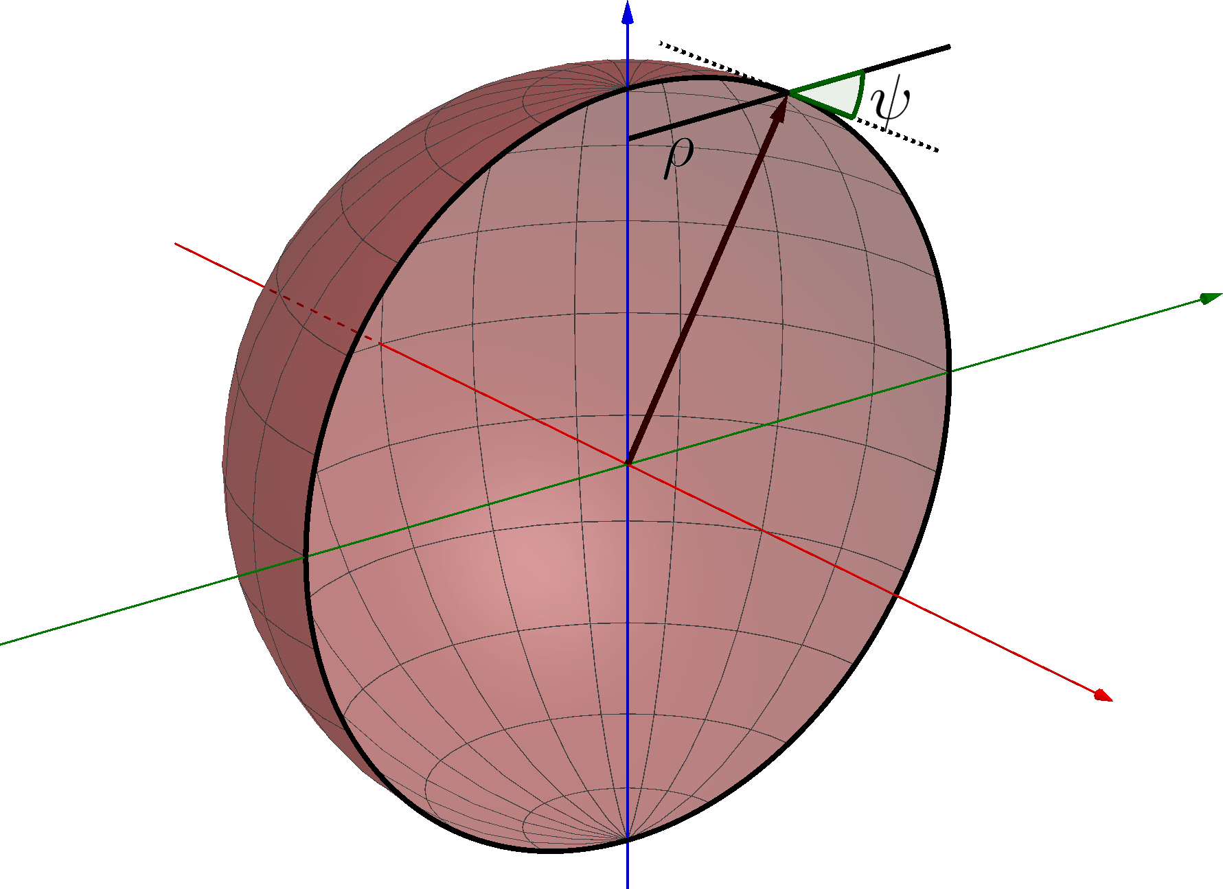
(a) Sphere

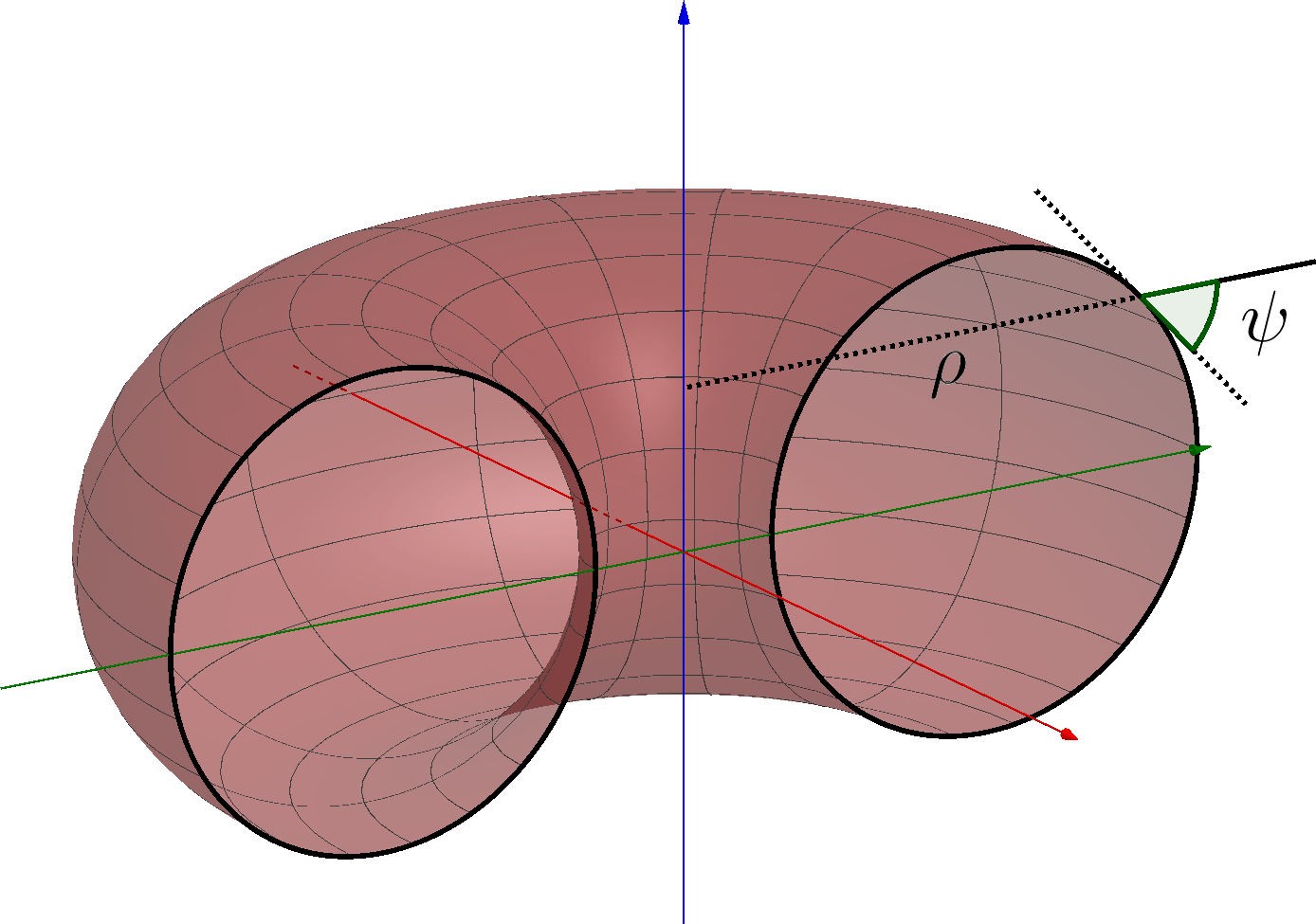
(b) Torus

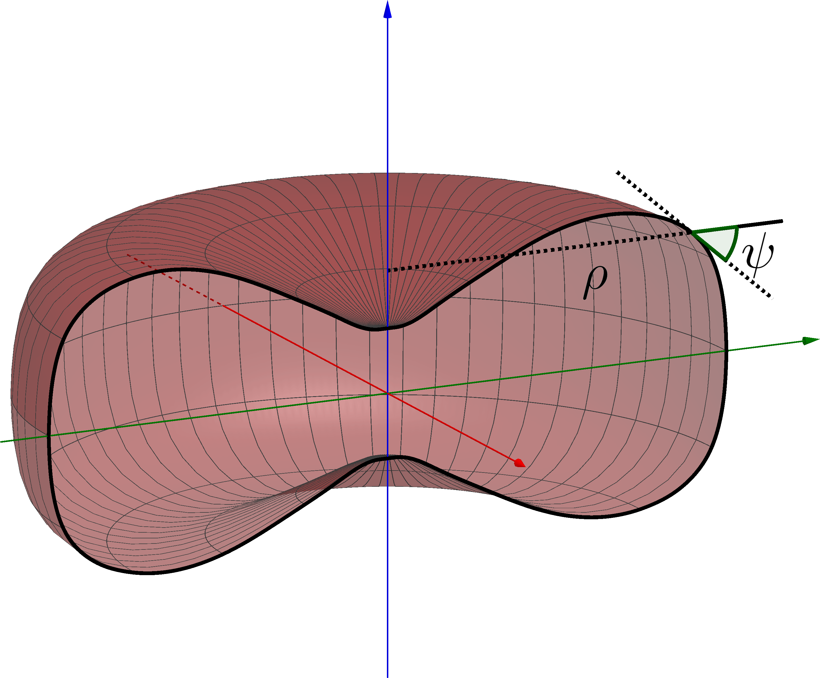
(c) Biconcave discoid

Figure 2: The three axisymmetric biophysical solutions to the Canham–Helfrich model and how they arise as surfaces of revolution. The coordinate $\rho$ measures the perpendicular distance to the $z$-axis (blue), while $\psi$ is the angle between the tangent of the contour and the $\rho$-axis.

Spherical vesicle:

A sphere of radius $R$ (see figure 2(a)) is described by

$$\sin\psi(\rho)=\frac{\rho}{R}~{}~{},$$ (4.141)

which gives rise to the equation

$$0=\Delta pR^{2}+4c_{0}\kappa+2c_{0}^{2}R\kappa+2R\lambda~{}~{}.$$ (4.142)

As was also pointed out in Tu and Ou-Yang (2014), this has two solutions when viewed as an equation for the radius, provided that $\Delta p<0$ and $-4c_{0}\kappa\Delta p+(\kappa c_{0}^{2}+\chi)^{2}>0$. The first condition reflects the fact that the internal pressure must be greater than the external pressure to stabilise the structure.

Torus:

The torus can also be obtained as a surface of revolution (figure 2(b)). This is achieved via

$$\sin\psi(\rho)=\frac{1}{r}\rho+\frac{R}{r}~{}~{},$$ (4.143)

where $R$ is the major axis and $r$ the minor axis. From this, we get the shape equation

$$0 = \left(-\kappa R^{3}+2\kappa r^{2}R\right)+\rho^{2}\left(r^{2}R\left(-\kappa{c_{0}}^{2}-\chi\right)-4\alpha{c_{0}}rR\right)$$ (4.144)

$$+\rho^{3}\left(-2r^{2}\left(\kappa{c_{0}}^{2}+\chi\right)+4\kappa{c_{0}}r+\Delta pr^{3}\right)~{}~{}.$$

Each coefficient of $\{\rho^{0},\rho^{2},\rho^{3}\}$ must vanish independently, giving us three equations

$$R=\sqrt{2}r~{}~{},~{}~{}\chi=\frac{\kappa c_{0}\left(4-c_{0}r\right)}{r}~{}~{},~{}~{}\Delta p=\frac{4\kappa c_{0}}{r^{2}}~{}~{}.$$ (4.145)

The first of these predicts a universal ratio between the major and minor axes. Theoretically predicted in Zhong-Can (1990), this ratio was observed experimentally in Mutz and Bensimon (1991) with high precision.

Biconcave discoid:

The biconcave discoid (figure 2(c)) is the shape of the red blood cell. This axisymmetric vesicle is described by

$$\sin\psi(\rho)=a\rho(\log\rho+b)~{}~{},$$ (4.146)

where $a,b$ are parameters that are related to the characteristics of the discoid. The resulting equation of motion is

$$0= \left(\kappa a^{3}-2\kappa a^{2}b-4\kappa ab^{2}+4\kappa abc_{0}-a\left(\kappa c_{0}^{2}+\chi\right)+4\kappa b^{2}c_{0}-2b\left(\kappa c_{0}^{2}+\chi\right)+\Delta p\right)$$

$$+\log\rho\left(-2\kappa a^{3}-8\kappa a^{2}b+4\kappa a^{2}c_{0}+8\kappa abc_{0}-2a\left(\kappa c_{0}^{2}+\chi\right)\right)$$

$$+\log^{2}\rho\left(-4a^{3}\kappa+4a^{2}\kappa c_{0}\right)\,,$$ (4.147)

which again gives three equations. These equations yield

$$a=c_{0}~{}~{},~{}~{}\chi=\Delta p=0~{}~{}.$$ (4.148)

Thus, we recover the result that the biconcave shape of the red blood cell relies on isotonicity, i.e. that the pressures on each side of the membrane are equal Naito et al. (1996) (see also Tanford (1979)).

5 Discussion & outlook

The majority of the work presented here was of a foundational nature. In order to describe the physical properties of fluid membranes in thermodynamic equilibrium, we developed the submanifold calculus for Newton–Cartan geometry. This parallels how the submanifold calculus of (pseudo-)Riemannian/Euclidean geometry is a pre-requisite for formulating and varying the standard Canham-Helfrich bending energy. We identified the geometric structures characterising timelike submanifolds in NC geometry and obtained the associated integrability conditions. Deriving expressions for the infinitesimal variations and transformation properties of the basic objects allowed us to formulate a generic extremisation problem for broad classes of NC surfaces, including fluid membranes whose equilibrium configurations only depend on geometric properties.

In section 4, we applied this newly developed toolbox to the description of fluid membranes in thermodynamic equilibrium. The novel aspect of these applications is that the dependence on temperature and chemical potential of material coefficients, such as surface tension and bending modulus, is critical for the emergence of wave excitations. This relied on the fact that temperature and chemical potential have a geometric interpretation related to the existence of a timelike isometry in the ambient spacetime. Standard examples of free energies such as the Canham-Helfrich bending energy are straightforwardly generalised by taking into account the geometric interpretation of thermodynamic variables. The resulting free energies are still purely geometric but the derived stresses on the membrane are different than standard results found in the literature. In particular, the Gaussian bending modulus can play a role in the shape of lipid vesicles since the Gaussian curvature cannot be integrated out when material coefficients are not constant. The resulting stresses produce elastic waves when perturbing away from equilibrium thus providing the correct dynamics of fluid membranes.

This paves the way for tackling several open questions, which we plan to address in a future publication Armas et al. :

• The fact that the Gaussian curvature cannot be integrated out in thermal equilibrium suggests that the family of closed lipid vesicles reviewed in section 4.2.3 should be revisited and the effects of the Gaussian bending modulus should be considered (i.e. $a_{3}$ in (4.131)), including the effects on deviations away from equilibrium.

• The lipid vesicle solutions in section 4.2.3 are static solutions, in which $u^{a}=(1,0,0)$. However, in principle such solutions can sustain rotation along the direction $\phi$. The question is thus: is it possible to obtain lipid vesicles with stationary flows?

• From an effective field theory point of view, the Canham–Helfrich bending energy (4.131) does not contain all possible responses that take into account thermal equilibrium. For instance a term quadratic in the extrinsic curvature of the form $u^{a}u^{b}h^{cd}{K_{bc}}K_{ad}$ involving the fluid velocity can be added to (4.131) (similarly to its relativistic counterpart Armas (2013)). However, there are further couplings that involve derivatives of $u_{a}$ such as the square of the fluid acceleration $(u^{a}\mathfrak{D}_{a}u^{b})^{2}$ or the square of the vorticity. Some of these terms are related to the Gaussian curvature and thus, by the Gauss-Codazzi equation (2.73), to combinations of squares of the extrinsic curvature. Therefore, from an effective theory point of view, they cannot be ignored a priori.

• We have shown in section 4.1.2 that taking into account the geometric definitions of temperature and mass chemical potential in equilibrium gives rise to the correct dispersion relation for an elastic membrane when perturbing away from equilibrium. It would now be interesting to consider perturbations away from equilibrium solutions of the Canham–Helfrich model (4.131) using the stresses (4.132)-(4.135). This would shed light on the stability of lipid vesicles.

• The construction of effective actions or free energies in the manner described in this work is appropriate to describe equilibrium configurations. However, including different types of dissipation Napoli and Vergori (2016), either due to viscous flows or diffusion of embedded proteins is of interest Steigmann (2018). In order to include dissipation from an effective action point of view one could consider the more elaborate Schwinger-Keldysh framework Haehl et al. (2016); Jensen et al. (2018); Liu and Glorioso (2018) and adapt it to non-relativistic systems. Alternatively, one may construct the effective theory in a long-wavelength hydrodynamic expansion by classifying potential terms appearing in the currents $\mathcal{T}^{a}$ and $\mathcal{T}^{ab}$ and obtaining constitutive relations (see e.g. Kovtun (2012); Armas (2014)). We plan on addressing this in the near future.

• We focused on extrinsic curvature terms in effective actions (3.98) but it would also be interesting to consider the effect of the external rotation tensor (2.63). In the (pseudo-)Riemannian/Euclidean setting, this corresponds to spinning point particles/membranes Guven (2007); Armas (2013); Armas and Harmark (2014b); Armas and Tarrio (2018) and are directly related to the Frenet curvature and Euler elastica (see e.g.  Guven (2019a); Guven and Manrique (2019); Guven (2019b) for a recent discussion).

• In sections 2 and 3 we formulated the description of a single surface in Newton–Cartan geometry for which the scalars $X^{\mu}$ can be seen as Goldstone modes of spontaneous broken translations at the location of the surface. It would be interesting to extend this further to the case of a foliation of surfaces, in which case the scalars $X^{\mu}$ form a lattice and can be used to describe viscoelasticity as in Armas and Jain (2019).

In this work we considered Newton–Cartan geometry but there are many other types of non-Lorentzian geometries depending on the space-time symmetry group, which can be e.g. Lifshitz, Schrödinger or Aristotelian, which have direct applications for the hydrodynamics of strongly correlated electron systems as well as for the hydrodynamics of flocking behaviour and active matter de Boer et al. (2018a, b); Poovuttikul and Sybesma (2019); Novak et al. (2019). In these contexts, it is required to develop the mathematical description of submanifolds within these different types of ambient spacetimes. The description of surfaces within these geometries will be of interest for surface/edge physics in hard condensed matter.

Appendix A Null reduction of Riemannian surfaces and perfect fluids

In this appendix we provide a completely different approach to formulating the theory of surfaces and fluid membranes in Newton–Cartan geometry. This approach consists in starting from relativistic surfaces and fluid membranes and performing a null reduction so as to obtain results in NC geometry. The purpose of this technical appendix is to provide a non-trivial check of the main results in the core of this paper.

A.1 Submanifolds from null reduction

It is well known that any Newton–Cartan geometry can be obtained as the null reduction of a Lorentzian manifold in one dimension higher equipped with a null killing vector Julia and Nicolai (1995); Christensen et al. (2014b); Hartong et al. (2016). Therefore, if we choose a timelike submanifold in a Lorentzian geometry such that the null Killing vector is tangent to the submanifold, its null reduction provides us with a Newton–Cartan submanifold embedded in a Newton–Cartan ambient spacetime. We illustrate this in the commuting diagram below:

$$\begin{CD}(\widehat{\Sigma}_{p+2},\hat{\gamma})@<{{\hat{u}}^{\hat{\mu}}_{\hat{a}}}<{}<(\widehat{\mathcal{M}}_{d+2},\hat{g})\\ @V{\text{null red.}}V{}V@V{}V{\text{null red.}}V\\ (\Sigma_{p+1},\{\tau|_{\Sigma},\check{h},\check{m}\})@<{}<{u^{\mu}_{a}}<(\mathcal{M}_{d+1},\{\tau,h,m\})\end{CD}$$ (A.149)

In section 2.2, we described how to go from the NC manifold $(\mathcal{M}_{d+1},\{\tau,h,m\})$ to the NC submanifold $(\Sigma_{p+1},\{\tau|_{\Sigma},\check{h},\check{m}\})$, while passing from the Lorentzian manifold $(\widehat{\mathcal{M}}_{d+2},\hat{g})$ to the Newton–Cartan manifold $(\mathcal{M}_{d+1},\{\tau,h,m\})$ is achieved by null reduction.

In this appendix, we will traverse the other route: our goal is to go from $(\widehat{\mathcal{M}}_{d+2},\hat{g})$ to $(\Sigma_{p+1},\{\tau|_{\Sigma},\check{h},\check{m}\})$ via $(\widehat{\Sigma}_{p+2},\hat{\gamma})$. The procedure to go from $(\widehat{\mathcal{M}}_{d+2},\hat{g})$ to $(\widehat{\Sigma}_{p+2},\hat{\gamma})$ is nothing but the theory of submanifolds in Lorentzian geometry and is well known (see e.g. Armas (2013); Armas and Tarrio (2018)). We coordinatise $\widehat{\mathcal{M}}_{d+2}$ with $x^{\hat{\mu}}=(u,x^{\mu})$ and $\widehat{\Sigma}_{p+2}$ with $\hat{\sigma}^{\hat{a}}=(w,\sigma^{a})$. The metric on $\widehat{\mathcal{M}}_{d+2}$ can – by assumption – be written in null reduction form

$$ds_{\widehat{\mathcal{M}}_{d+2}}^{2}=\hat{g}_{\hat{\mu}\hat{\nu}}{\text{d}x}^{\hat{\mu}}{\text{d}x}^{\hat{\nu}}=2\tau_{\mu}{\text{d}x}^{\mu}(\text{d}u-m_{\nu}{\text{d}x}^{\nu})+h_{\mu\nu}{\text{d}x}^{\mu}{\text{d}x}^{\nu}~{}~{}.$$ (A.150)

This line element is invariant under the Newton–Cartan gauge transformations (2.4) and conversely all gauge invariance of this line element are of the form (2.4). The invariance under the $U(1)$ transformation with parameter $\sigma(x^{\mu})$ requires that we vary the higher-dimensional coordinate $u$ as $\delta u=\sigma$. From the higher-dimensional perspective this corresponds to a diffeomorphism that leaves the $x^{\mu}$ unaffected but that shifts $u$ by some function of $x^{\mu}$.

The Lorentzian submanifold is defined via a set of embedding maps $\hat{X}^{\hat{\mu}}(\sigma^{\hat{a}})$ in the usual way. We define the projector

$$\hat{P}^{\hat{\mu}}_{\hat{\nu}}=\hat{u}^{\hat{\mu}}_{\hat{a}}\hat{u}_{\hat{\nu}}^{\hat{a}}=\delta^{\hat{\mu}}_{\hat{\nu}}-\hat{n}^{I}_{\hat{\rho}}\hat{n}^{J}_{\hat{\nu}}\delta_{IJ}\hat{g}^{\hat{\rho}\hat{\mu}}~{}~{},$$ (A.151)

where $\hat{n}^{I}_{\hat{\rho}}$ are the normal one-forms to $\widehat{\Sigma}_{p+2}$ and where $\hat{u}^{\hat{\mu}}_{\hat{a}}={\partial}_{\hat{a}}\hat{X}^{\hat{\mu}}$. We require that the null direction is shared between $\widehat{\mathcal{M}}_{d+2}$ and $\widehat{\Sigma}_{p+2}$, which can be expressed as the requirements

$$\hat{u}^{u}_{w}=1~{}~{},~{}~{}\hat{u}^{u}_{a}=0~{}~{},$$ (A.152)

where the null direction on the submanifold is described by $w$. Further, we want to impose a null reduction analogue of the timelike requirement (2.24). To this end, we introduce a vector $U^{\hat{\mu}}=\left(\frac{\partial}{\partial u}\right)^{\hat{\mu}}=\delta^{\hat{\mu}}_{u}$ so that $U_{\hat{\mu}}=(0,\tau_{\mu})$. Requiring that the null Killing vector field is tangential to the submanifold $\hat{n}_{u}^{I}=U^{\hat{\mu}}\hat{n}^{I}_{\hat{\mu}}=U_{\hat{\mu}}\hat{n}^{\hat{\mu}I}=0$ for all $I$ implies the desired relation $\tau_{\mu}n^{\mu}_{I}=0$ where we have identified $\hat{n}^{\mu}_{I}=n^{\mu}_{I}$. This further implies that $n^{\mu I}=\hat{g}^{\mu\hat{\nu}}\hat{n}^{I}_{\hat{\nu}}=h^{\mu\nu}n^{I}_{\nu}$ in agreement with the timelike constraint. This also implies that $\hat{P}^{\mu}_{\nu}=P^{\mu}_{\nu}$, as well as the normalisation $\hat{g}^{\hat{\mu}\hat{\nu}}\hat{n}^{I}_{\hat{\mu}}\hat{n}^{J}_{\hat{\nu}}=h^{\mu\nu}n^{I}_{\mu}n^{J}_{\nu}=\delta^{IJ}$. Further, the above considerations lead us to conclude that

$$\hat{n}^{uI}=\hat{g}^{u\hat{\mu}}\hat{n}^{I}_{\hat{\mu}}=-\hat{v}^{\mu}n^{I}_{\mu}=-\hat{v}^{I}\,.$$ (A.153)

The metric on $\widehat{\Sigma}_{p+2}$ can also be written in null reduction form

$$ds_{\widehat{\Sigma}_{p+2}}^{2}=\hat{\gamma}_{\hat{a}\hat{b}}{\text{d}x}^{\hat{a}}{\text{d}x}^{\hat{b}} = 2\tau_{a}{\text{d}x}^{a}(\text{d}w-m_{b}{\text{d}x}^{b})+h_{ab}{\text{d}x}^{a}{\text{d}x}^{b}$$ (A.154)

$$= 2\tau_{a}{\text{d}x}^{a}(\text{d}w-\check{m}_{b}{\text{d}x}^{b})+\check{h}_{ab}{\text{d}x}^{a}{\text{d}x}^{b}~{}~{},$$

where we recall the definitions of $\check{h}_{ab}$ and $\check{m}_{a}$ in (2.34) and (2.39), respectively. As manifested in the equations above, the null reduction form of the metric is Galilean boost-invariant and does not distinguish between checked and un-checked metric data. In turn, the Lorentzian metric $\hat{\gamma}$ on $\widehat{\Sigma}_{p+2}$ is the pullback of the metric $\hat{g}$ on $\widehat{\mathcal{M}}_{d+2}$, that is

$$\hat{\gamma}_{\hat{a}\hat{b}}=\hat{u}^{\hat{\mu}}_{\hat{a}}\hat{u}^{\hat{\nu}}_{\hat{b}}\hat{g}_{\hat{\mu}\hat{\nu}}~{}~{},$$ (A.155)

which implies that

$$\tau_{a}=\hat{\gamma}_{aw}=\hat{u}^{\hat{\mu}}_{a}\hat{u}^{\hat{\nu}}_{w}\hat{g}_{\hat{\mu}\hat{\nu}}=\hat{u}^{\mu}_{a}\hat{u}^{u}_{w}\hat{g}_{\mu u}+\hat{u}^{\mu}_{a}\hat{u}^{\nu}_{w}\hat{g}_{\mu\nu}=\hat{u}^{\mu}_{a}\tau_{\mu}+\hat{u}^{\mu}_{a}\hat{u}^{\nu}_{w}\bar{h}_{\mu\nu}~{}~{}.$$ (A.156)

Thus, taking

$$\hat{u}^{\mu}_{w}=0~{}~{},$$ (A.157)

and identifying $\hat{u}^{\mu}_{a}={u}^{\mu}_{a}$ we get the desired relation between the two clock 1-forms, namely $\tau_{a}=u^{\mu}_{a}\tau_{\mu}$. Next, we consider

$$\bar{h}_{ab}=\hat{\gamma}_{ab}=\hat{u}^{\hat{\mu}}_{a}\hat{u}^{\hat{\nu}}_{b}\hat{g}_{\hat{\mu}\hat{\nu}}=\hat{u}^{\mu}_{a}\hat{u}^{\nu}_{b}\hat{g}_{\mu\nu}+\hat{u}^{\mu}_{a}\hat{u}^{u}_{b}\hat{g}_{\mu u}+\hat{u}^{u}_{a}\hat{u}^{\nu}_{b}\hat{g}_{u\nu}=u^{\mu}_{a}u^{\nu}_{b}\bar{h}_{\mu\nu}~{}~{},$$ (A.158)

where we have used (A.152), which again agrees with the results of section 2.2. The relation $\hat{u}^{\hat{\mu}}_{w}\hat{u}^{w}_{\hat{\mu}}=\hat{u}^{w}_{u}=1$ where we used (A.157), fixes $\hat{u}^{w}_{u}=1$. To determine $\hat{u}^{w}_{\mu}$ we bring into play the orthogonality requirement $\hat{u}^{w}_{\hat{\mu}}\hat{n}^{\hat{\mu}I}=\hat{g}^{\hat{\mu}\hat{\nu}}\hat{u}^{w}_{\hat{\mu}}\hat{n}^{I}_{\hat{\nu}}=0$, which translates into the relation

$$\hat{v}^{\mu}n^{I}_{\mu}=\hat{u}^{w}_{\mu}n^{\mu I}~{}~{},$$ (A.159)

where we have used that $\hat{u}^{w}_{u}=1$ and $n^{\mu}_{I}=\delta_{IJ}h^{\mu\nu}n^{J}_{\nu}$. This is only possible if

$${\hat{u}^{w}_{\mu}=\hat{v}^{I}n^{I}_{\mu}~{}~{}.}$$ (A.160)

The null reduction of the ambient inverse metric is

$$\hat{g}^{uu}=2\tilde{\Phi}~{}~{},~{}~{}\hat{g}^{u\mu}=-\hat{v}^{\mu}~{}~{},~{}~{}\hat{g}^{\mu\nu}=h^{\mu\nu}~{}~{},$$ (A.161)

while the relation between $\hat{g}^{-1}$ and $\hat{\gamma}^{-1}$ is given by $\hat{\gamma}^{\hat{a}\hat{b}}=\hat{u}^{\hat{a}}_{\hat{\mu}}\hat{u}^{\hat{b}}_{\hat{\nu}}\hat{g}^{\hat{\mu}\hat{\nu}}$. In turn, the relation $\hat{\gamma}^{ab}=h^{ab}$ requires that $\hat{u}^{a}_{u}=0$. Using this, we can write

$$\hat{\gamma}^{wa}=\hat{u}^{w}_{\hat{\mu}}\hat{u}^{a}_{\hat{\nu}}\hat{g}^{\hat{\mu}\hat{\nu}}=\hat{v}^{I}n^{I}_{\mu}\hat{u}^{a}_{\nu}h^{\mu\nu}+\hat{u}^{a}_{\nu}\hat{g}^{u\nu}\,,$$ (A.162)

where we have used (A.160), which leads us to identify $\hat{u}^{a}_{\mu}=u^{a}_{\mu}$ and, by the orthogonality relation (2.25), leads to $\hat{v}^{a}=u^{a}_{\mu}\hat{v}^{\mu}$ as desired. The relation (A.160) furthermore implies that

$$\hat{\gamma}^{ww}=\hat{u}^{w}_{\hat{\mu}}\hat{u}^{w}_{\hat{\nu}}\hat{g}^{\hat{\mu}\hat{\nu}}=2\tilde{\Phi}-\hat{v}^{I}\hat{v}_{I}=\check{\Phi}~{}~{}.$$ (A.163)

In summary, the Lorentzian objects arrange themselves under submanifold null reduction according to

$$\hat{u}^{\hat{\mu}}_{\hat{a}} \overset{\text{null red.}}{\longrightarrow}\qquad\hat{u}^{\mu}_{a}=u^{\mu}_{a}~{}~{},~{}~{}\hat{u}^{u}_{w}=1~{}~{},~{}~{}\hat{u}^{\mu}_{w}=0~{}~{},~{}~{}\hat{u}^{u}_{a}=0~{}~{},$$ (A.164)

$$\hat{u}_{\hat{\mu}}^{\hat{a}} \overset{\text{null red.}}{\longrightarrow}\qquad\hat{u}^{a}_{\mu}=u^{a}_{\mu}~{}~{},~{}~{}\hat{u}^{w}_{u}=1~{}~{},~{}~{}\hat{u}^{w}_{\mu}=\hat{v}^{I}n^{I}_{\mu}~{}~{},~{}~{}\hat{u}^{a}_{u}=0~{}~{},$$ (A.165)

$$\hat{n}^{I}_{\hat{\mu}} \overset{\text{null red.}}{\longrightarrow}\qquad\hat{n}^{I}_{\mu}=n^{I}_{\mu}~{}~{},~{}~{}\hat{n}^{I}_{u}=0~{}~{},$$ (A.166)

$$\hat{n}_{I}^{\hat{\mu}} \overset{\text{null red.}}{\longrightarrow}\qquad\hat{n}_{I}^{\mu}=n_{I}^{\mu}~{}~{},~{}~{}\hat{n}_{I}^{u}=-\hat{v}_{I}~{}~{}.$$ (A.167)

The metric on $\widehat{\Sigma}_{p+2}$ is

$$ds_{\widehat{\Sigma}_{p+2}}^{2}=2\tau_{a}{\text{d}x}^{a}(\text{d}w-\check{m}_{b}{\text{d}x}^{b})+\check{h}_{ab}{\text{d}x}^{a}{\text{d}x}^{b}~{}~{},$$ (A.168)

while the components of the inverse metric on $\widehat{\Sigma}_{p+2}$ are

$${\hat{\gamma}^{ww}=2\check{\Phi}=2\tilde{\Phi}-\hat{v}^{I}\hat{v}^{I},\qquad\hat{\gamma}^{wa}=-\hat{v}^{a},\qquad\hat{\gamma}^{ab}=h^{ab}~{}~{}.}$$ (A.169)

A.1.1 Null reduction of the connection & the extrinsic curvature

We now consider the null-reduction of the Lorentzian connection. The non-zero components of the higher-dimensional Christoffel symbols are

$$\hat{\Gamma}_{\mu\nu}^{\rho} = \bar{\Gamma}^{\rho}_{(\mu\nu)}=\bar{\Gamma}^{\rho}_{\mu\nu}+\frac{1}{2}\hat{v}^{\rho}\tau_{\mu\nu}~{}~{},$$ (A.170)

$$\hat{\Gamma}_{\mu\nu}^{u} = -\bar{\mathcal{K}}_{\mu\nu}-2\tau_{(\mu}{\partial}_{\nu)}\tilde{\Phi}~{}~{},$$ (A.171)

$$\hat{\Gamma}_{u\mu}^{\rho} = \frac{1}{2}h^{\rho\sigma}\tau_{\mu\sigma}~{}~{},$$ (A.172)

$$\hat{\Gamma}_{u\mu}^{u} = \frac{1}{2}a_{\mu}~{}~{},$$ (A.173)

where

$$\bar{\mathcal{K}}_{\mu\nu}=-\frac{1}{2}\pounds_{\hat{v}}\bar{h}_{\mu\nu}~{}~{},~{}~{}a_{\mu}=\pounds_{\hat{v}}\tau_{\mu}=\hat{v}^{\rho}\tau_{\rho\mu}~{}~{}.$$ (A.174)

The NC extrinsic curvature $\bar{\cal K}_{\mu\nu}$ should not be confused with the submanifold extrinsic curvature $K_{ab}{}^{I}$. The pullback of the ambient TNC extrinsic curvature, $\bar{\mathcal{K}}_{ab}=u^{\mu}_{a}u^{\nu}_{b}\bar{\mathcal{K}}_{\mu\nu}$, is related to the TNC extrinsic curvature on the submanifold $\Sigma_{p+1}$,

$$\bar{\mathcal{K}}^{\Sigma}_{ab}=-\frac{1}{2}\pounds^{\Sigma}_{\hat{v}}\bar{h}_{ab}~{}~{},$$ (A.175)

where $\pounds^{\Sigma}_{\hat{v}}$ denotes the Lie derivative along $\hat{v}^{a}$ on $\Sigma_{p+1}$, in the following way

$$\bar{\mathcal{K}}_{ab}=\bar{\mathcal{K}}^{\Sigma}_{ab}-\tau_{(a}\partial_{b)}(\hat{v}^{I}\hat{v}^{I})+\hat{v}^{I}K_{ab}{{}^{I}}~{}~{}.$$ (A.176)

This can be shown by starting with $\bar{\mathcal{K}}_{ab}=u^{\mu}_{a}u^{\nu}_{b}\bar{\mathcal{K}}_{\mu\nu}$ and using $\hat{v}^{\rho}=\hat{v}^{c}u_{c}^{\rho}+\hat{v}^{I}n^{\rho}_{I}$ in (A.174). The following identity

$$\pounds_{n^{I}}\bar{h}_{\mu\nu}=2\nabla_{(\mu}n_{\nu)}^{I}+2\tau_{(\mu}\partial_{\nu)}\hat{v}^{I}\,,$$ (A.177)

together with equation (2.61) can then be used to derive (A.176).

The higher-dimensional extrinsic curvature $\hat{K}_{\hat{a}\hat{b}}{{}^{I}}$ is determined in terms of the higher-dimensional analogue of the surface covariant derivative of (2.56), which we will call $\hat{D}_{\hat{a}}$. It acts on a mixed tensor $\hat{T}^{\hat{b}\hat{\mu}}$ according to

$$\hat{D}_{\hat{a}}\hat{T}^{\hat{b}\hat{\mu}}={\partial}_{\hat{a}}\hat{T}^{\hat{b}\hat{\mu}}+\hat{\gamma}^{\hat{b}}_{\hat{a}\hat{c}}\hat{T}^{\hat{c}\hat{\mu}}+\hat{u}^{\hat{\nu}}_{\hat{a}}\hat{\Gamma}^{\hat{\mu}}_{\hat{\nu}\hat{\lambda}}\hat{T}^{\hat{b}\hat{\lambda}}~{}~{},$$ (A.178)

where $\hat{\gamma}^{\hat{b}}_{\hat{a}\hat{c}}$ is the Levi-Civita connection of $\hat{\gamma}$, while $\hat{\Gamma}^{\hat{\mu}}_{\hat{\nu}\hat{\lambda}}$ is the Levi-Civita connection of $\hat{g}$. The higher-dimensional extrinsic curvature is

$$\hat{K}_{\hat{a}\hat{b}}{{}^{I}}=\hat{n}_{\hat{\mu}}^{I}\hat{D}_{\hat{a}}\hat{u}^{\hat{\mu}}_{\hat{b}}=\hat{n}_{\hat{\mu}}^{I}\left({\partial}_{\hat{a}}\hat{u}^{\hat{\mu}}_{\hat{b}}+\hat{u}^{\hat{\nu}}_{\hat{a}}\hat{\Gamma}^{\hat{\mu}}_{\hat{\nu}\hat{\lambda}}\hat{u}^{\hat{\lambda}}_{\hat{b}}\right)~{}~{},$$ (A.179)

which using (A.164) and (A.166) means that

$$\hat{K}_{ab}{{}^{I}}=n_{\mu}^{I}D_{a}u^{\mu}_{b}+\frac{1}{2}\hat{v}^{I}{\tau_{ab}}=K_{ab}{{}^{I}}\,,$$ (A.180)

where we have recognised the extrinsic curvature of (2.61). This is invariant under both gauge transformations and Galilean boosts. The other non-zero components of the higher-dimensional extrinsic curvature are $\hat{K}_{wb}{}^{I}=-\frac{1}{2}\tau_{Ib}$.

Below equation (A.150), we have shown that the $U(1)$ gauge transformation is a specific diffeomorphism in the higher-dimensional description. This is a useful way to find out how various objects transform under the $\sigma$ gauge transformation. This also applies to tensors defined on the submanifold $\Sigma_{p+1}$, since they descend from the Lorentzian manifold $\widehat{\Sigma}_{p+2}$. A diffeomorphism of a generic tensor $X_{\hat{a}}{}^{\hat{b}}$ is given by

$$\delta X_{\hat{a}}{}^{\hat{b}}=\hat{\xi}^{\hat{c}}\partial_{\hat{c}}X_{\hat{a}}{}^{\hat{b}}+X_{\hat{c}}{}^{\hat{b}}\partial_{\hat{a}}\hat{\xi}^{\hat{c}}-X_{\hat{a}}{}^{\hat{c}}\partial_{\hat{c}}\hat{\xi}^{\hat{b}}~{}~{}.$$ (A.181)

In order to find the $U(1)$ transformation, we need to choose a diffeomorphism for which $\hat{\xi}^{\hat{a}}=-\sigma\delta^{\hat{a}}_{w}$. Since all objects are independent of $u$ we find that a one-form $X_{a}$ in this case transforms as

$$\delta X_{a}=-X_{w}\partial_{a}\sigma~{}~{},$$ (A.182)

while a vector $X^{b}$ is $U(1)$ invariant. Applying this to the extrinsic curvature $\hat{K}_{ab}{{}^{I}}$ we find

$$\delta_{\sigma}\hat{K}_{ab}{{}^{I}}=-\hat{K}_{aw}{{}^{I}}\partial_{b}\sigma-\hat{K}_{wb}{{}^{I}}\partial_{a}\sigma~{}~{}.$$ (A.183)

Using that $\hat{K}_{wb}{}^{I}=-\frac{1}{2}\tau_{Ib}$ we recover the transformation rule (2.62).

A.1.2 Variations from null reduction

Here we obtain some of the results of section 3.1 using null reduction. We begin with the variations of the normal 1-forms. In the relativistic case, the normal 1-forms can be shown to transform as Armas and Tarrio (2018)

$$\delta\hat{n}^{I}_{\hat{\mu}}=\frac{1}{2}\hat{n}^{\hat{\nu}}_{J}\hat{n}^{J}_{\hat{\mu}}\hat{n}^{{\hat{\rho}}I}\delta\hat{g}_{\hat{\nu}\hat{\rho}}-\hat{n}^{I}_{\hat{\nu}}\hat{u}^{\hat{a}}_{\hat{\mu}}\delta\hat{u}^{\hat{\nu}}_{\hat{a}}+\frac{1}{2}\hat{n}_{\hat{\mu}J}(\hat{n}^{\hat{\nu}J}\delta\hat{n}^{I}_{\hat{\nu}}-\hat{n}^{\hat{\nu}I}\delta\hat{n}^{J}_{\hat{\nu}})~{}~{}.$$ (A.184)

Restricting to $\hat{\mu}=\mu$, the last term simply reduces to $\lambda^{I}{}_{J}n_{\mu}^{J}$. This follows from demanding that $\hat{n}^{I}_{u}=0$ is preserved under transformations, implying that $\delta\hat{n}^{I}_{u}=0$. Ignoring rotations of the normal one-forms, we get

$$\delta n^{I}_{\mu}=-\frac{1}{2}\hat{v}^{\rho}n^{J}_{\rho}n_{\mu J}n^{\nu I}\delta\tau_{\nu}-\frac{1}{2}n^{\nu J}n_{\mu J}\hat{v}^{\rho}n^{I}_{\rho}\delta\tau_{\nu}+\frac{1}{2}{n}^{\rho J}n_{\mu J}n^{\nu I}\delta\bar{h}_{\rho\nu}-{n}^{I}_{\nu}u^{a}_{\mu}\delta u^{\nu}_{a}~{}~{},$$ (A.185)

where we have used that $\hat{n}^{uI}=-\hat{v}^{\mu}n^{I}_{\mu}$. Using the definitions of $\hat{v}$ and $\bar{h}$, we find that the variation can be written as

$${\delta n^{I}_{\mu}=-v^{(I}n^{J)\nu}n_{\mu J}\delta\tau_{\nu}+\frac{1}{2}n^{\rho J}n_{\mu J}n^{\nu I}\delta h_{\rho\nu}-{n}^{I}_{\nu}u^{a}_{\mu}\delta u^{\nu}_{a}~{}~{},}$$ (A.186)

in agreement with the result (3.79) (up to a local $\mathfrak{so}(d-p)$ transformation that we ignored).

With this at hand, we rederive (3.85) using the method of null reduction. The relativistic result reads Armas and Tarrio (2018)

$$\delta_{\hat{X}}\hat{K}_{\hat{a}\hat{b}}{{}^{I}}=-\hat{n}_{\hat{\mu}}^{I}\hat{D}_{\hat{a}}\hat{D}_{\hat{b}}\hat{\xi}^{\hat{\mu}}+\hat{n}_{\hat{\mu}}^{I}\hat{\xi}^{\hat{\lambda}}\hat{u}^{\hat{\nu}}_{\hat{a}}\hat{u}^{\hat{\rho}}_{\hat{b}}\hat{R}_{\hat{\lambda}\hat{\nu}\hat{\rho}}{{}^{\hat{\mu}}}+\hat{\lambda}^{I}{}_{J}\hat{K}_{\hat{a}\hat{b}}{{}^{J}}~{}~{},$$ (A.187)

where

$$\hat{\lambda}^{IJ}=\hat{n}^{\hat{\mu}[I}\hat{n}^{J]\hat{\nu}}\hat{\xi}^{\hat{\rho}}{\partial}_{\hat{\nu}}\hat{g}_{\mu\hat{\rho}}=\hat{n}_{\hat{\rho}}^{[I}\hat{n}^{J]\hat{\nu}}\hat{\Gamma}^{\hat{\rho}}_{\hat{\nu}\hat{\sigma}}\hat{\xi}^{\hat{\sigma}}\,.$$ (A.188)

We keep the null direction fixed, so that

$$\hat{\xi}^{\hat{\mu}}=-\delta\hat{X}^{\hat{\mu}}~{}~{},~{}~{}\hat{\xi}^{u}=0~{}~{}.$$ (A.189)

We are interested in $(\hat{a},\hat{b})=(a,b)$ and since $\hat{n}^{I}_{u}=0=\hat{u}^{u}_{a}$, (A.187) reduces to

$$\delta_{X}\hat{K}_{ab}{{}^{I}}=-n_{\mu}^{I}\hat{D}_{a}\hat{D}_{b}{\xi}^{\mu}+n_{\mu}^{I}\xi^{\lambda}{u}^{\nu}_{a}u^{\sigma}_{b}\hat{R}_{\lambda\nu\sigma}{{}^{\mu}}+\hat{\lambda}^{I}{}_{J}\hat{K}_{ab}{{}^{J}}~{}~{},$$ (A.190)

where $\hat{\xi}^{\mu}=\xi^{\mu}$ so that $\delta\hat{X}^{\mu}=\delta X^{\mu}$. In the absence of torsion, the null reduction of the Riemann tensor gives

$$\hat{R}_{\lambda\nu\sigma}{{}^{\mu}}=-{\partial}_{\lambda}\hat{\Gamma}^{\mu}_{\nu\sigma}+{\partial}_{\nu}\hat{\Gamma}^{\mu}_{\lambda\sigma}-\hat{\Gamma}^{\mu}_{\lambda\hat{\rho}}\hat{\Gamma}^{\hat{\rho}}_{\nu\sigma}+\hat{\Gamma}^{\mu}_{\nu\hat{\rho}}\hat{\Gamma}^{\hat{\rho}}_{\lambda\sigma}=R_{\lambda\nu\sigma}{{}^{\mu}}~{}~{}.$$ (A.191)

Since in the absence of torsion $\hat{D}_{w}\xi^{\mu}=0$ and $\hat{D}_{b}\xi^{\mu}={D}_{b}\xi^{\mu}$, we find that

$$\hat{D}_{a}\hat{D}_{b}{\xi}^{\mu}={D}_{a}{D}_{b}{\xi}^{\mu}~{}~{},$$ (A.192)

while the null reduction of (A.188) gives $\hat{\lambda}^{IJ}=n_{\rho}^{[I}n^{J]\nu}\Gamma^{\rho}_{\nu\sigma}\xi^{\sigma}$ and so we obtain (3.85), as expected.

A.1.3 Note on the reduction of the Lorentzian action

The variational principle for NC surfaces in section 3.2.1 can be obtained from null reduction of the relativistic variational principle Armas (2013), namely

$$\delta S=\int_{\Sigma}\text{d}^{p+1}\sigma\sqrt{-\hat{\gamma}}\left(\frac{1}{2}\hat{T}^{\hat{a}\hat{b}}\delta\hat{\gamma}_{\hat{a}\hat{b}}+\hat{\mathcal{D}}^{\hat{a}\hat{b}}{{}_{I}}\delta\hat{K}_{\hat{a}\hat{b}}{{}^{I}}\right)~{}~{}.$$ (A.193)

The null reduction formulae of the previous section, for instance (A.190), imply that the null reduction of (A.193) will include a dependence on variations of $\hat{K}_{wa}{}^{I}=-\frac{1}{2}\tau_{Ib}$. Such torsion dependent terms were not included in (3.98). The reason, as mentioned throughout the paper is that we have assumed to be working without torsion, that is $\tau_{\mu\nu}=0$ at the expense of only being able to extract the divergence of the energy current instead of the energy current itself.

A.2 Perfect fluid from null reduction

In this section, we consider the null reduction of the equilibrium partition function of a relativistic space-filling perfect fluid, that is a fluid that is not living on a surface. The case in which the fluid is confined to the surface (i.e. a fluid membrane) considered in section 4.1 is a straightforward modification of this analysis. The result provides us with the hydrostatic partition function of a Galilean-invariant perfect fluid.

We begin with the null reduction of the unit normalised relativistic fluid velocity $\hat{u}^{\hat{\mu}}$, which obeys $\hat{g}_{\hat{\mu}\hat{\nu}}\hat{u}^{\hat{\mu}}\hat{u}^{\hat{\nu}}=-1$. We define the non-relativistic fluid velocity $u^{\mu}$ as follows Hartong et al. (2016),

$$u^{\mu}=\frac{\hat{u}^{\mu}}{\hat{u}_{u}}~{}~{},$$ (A.194)

where $\hat{u}_{u}=\hat{g}_{u\hat{\mu}}\hat{u}^{\hat{\mu}}=\tau_{\mu}\hat{u}^{\mu}$. This implies that $\tau_{\mu}u^{\mu}=1$ which is the standard normalisation of the contravariant velocity of a non-relativistic fluid. The relativistic condition

$$\hat{g}_{\hat{\mu}\hat{\nu}}\hat{u}^{\hat{\mu}}\hat{u}^{\hat{\nu}}=\bar{h}_{\mu\nu}\hat{u}^{\mu}\hat{u}^{\nu}+2\tau_{\mu}\hat{u}^{\mu}\hat{u}^{u}=-1~{}~{},$$ (A.195)

can be used to solve for $\hat{u}^{u}$, leading to

$$\hat{u}^{u}=-\frac{1}{2\hat{u}_{u}}-\frac{1}{2}\hat{u}_{u}\bar{h}_{\mu\nu}u^{\mu}u^{\nu}~{}~{}.$$ (A.196)

We still need to find a lower-dimensional interpretation of $\hat{u}_{u}$. This can be achieved as follows. Let $\hat{T}^{\hat{\mu}}{}_{\hat{\nu}}$ be the energy-momentum tensor of the higher-dimensional relativistic theory. For a perfect fluid this is $\hat{T}^{\hat{\mu}}{}_{\hat{\nu}}=\left(\hat{E}+\hat{P}\right)\hat{u}^{\hat{\mu}}{}\hat{u}_{\hat{\nu}}+\hat{P}\delta^{\hat{\mu}}_{\hat{\nu}}$. The mass current of the null reduced theory is given by $\hat{T}^{\mu}{}_{u}$ (see for example Hartong et al. (2016)). In the lower-dimensional theory, this is equal to $nu^{\mu}$, where $n$ is the mass density. Comparing the two expressions yields

$$\hat{u}_{u}^{2}=\frac{n}{\hat{E}+\hat{P}}~{}~{}.$$ (A.197)

We will later find expressions for $\hat{E}$ and $\hat{P}$ in terms of the non-relativistic energy and pressure.

In the hydrostatic partition function approach for a relativistic fluid, one identifies the intensive fluid variables such as temperature and velocity with a timelike Killing vector of an otherwise arbitrary Lorentzian curved background geometry. By varying the metric while keeping the Killing vector fixed, one extracts the fluid energy-momentum tensor. This approach has been applied to non-relativistic fluids on a NC background in Jensen (2014b); Banerjee et al. (2015b) and here we will show how this follows from null reduction. In the higher-dimensional Lorentzian geometry, we assume the existence of a Killing vector $\hat{k}^{\hat{\mu}}$ such that

$$\hat{k}^{\hat{\mu}}=\hat{\beta}\hat{u}^{\hat{\mu}}~{}~{},$$ (A.198)

where $\hat{\beta}$ is the relativistic (inverse) temperature, and $\hat{u}^{\hat{\mu}}$ the relativistic fluid velocity. Just like in the Lorentzian setting, we will introduce a Newton–Cartan Killing vector $k^{\mu}$ that is proportional to the non-relativistic fluid velocity $u^{\mu}$ and that is timelike, where $\tau_{\mu}k^{\mu}$ relates to the non-relativistic temperature. Hence we write

$$k^{\mu}=\beta u^{\mu}~{}~{},$$ (A.199)

where $\beta=\tau_{\mu}k^{\mu}$ is the non-relativistic (inverse) temperature. The null reduction of $\hat{k}^{\hat{\mu}}$ is just $\hat{k}^{\hat{\mu}}=(\hat{k}^{u}\,,k^{\mu})=\beta\left(\hat{\mu},u^{\mu}\right)$, where we write $\hat{k}^{u}=\beta\hat{\mu}$ with $\hat{\mu}$ a parameter to be determined. This means that

$$\beta u^{\mu}=\hat{\beta}\hat{u}^{\mu}~{}~{}.$$ (A.200)

Now, since $\hat{k}^{\hat{\mu}}$ is a Killing vector, we have that

$$\pounds_{\hat{k}}\hat{g}_{\hat{\mu}\hat{\nu}}=0~{}~{},$$ (A.201)

which, after null reduction, turns into the statements

$${\pounds_{k}\tau_{\mu}=0~{}~{},~{}~{}\pounds_{k}\bar{h}_{\mu\nu}=-2\tau_{(\mu}{\partial}_{\nu)}\hat{k}^{u}~{}~{}.}$$ (A.202)

In a NC geometry a Killing vector is defined by setting to zero the transformations in (2.4) (and thus also implying that the variations in (2.7) give zero). Here $\hat{k}^{u}$ is thus a specific $U(1)$ gauge transformation parameter that is associated with the existence of a Killing vector.

The relativistic hydrostatic partition function at ideal order in derivatives is an integral of the pressure which depends on the intensive variables, i.e. scalar quantities built from the Killing vector. One of these is the norm of $\hat{k}^{\hat{\mu}}$ which relates to the relativistic temperature. However, in the case of null reduction we actually have, besides $\hat{k}^{\hat{\mu}}$, another Killing vector which is $U^{\hat{\mu}}=\left(\frac{\partial}{\partial u}\right)^{\hat{\mu}}$. Since $U^{\hat{\mu}}$ is null, we can form only one other scalar, namely

$$\hat{g}_{\hat{\mu}\hat{\nu}}U^{\hat{\mu}}\hat{k}^{\hat{\nu}}=\tau_{\mu}k^{\mu}=\beta~{}~{},$$ (A.203)

which is the non-relativistic (inverse) temperature. The other scalar is of course

$$-\hat{\beta}^{2}=\hat{g}_{\hat{\mu}\hat{\nu}}\hat{k}^{\hat{\mu}}\hat{k}^{\hat{\nu}}=\beta^{2}\left(2\hat{\mu}+\bar{h}_{\mu\nu}u^{\mu}u^{\nu}\right)~{}~{}.$$ (A.204)

This determines the proportionality between the relativistic and non-relativistic temperatures. We define

$$\mu=\hat{\mu}+\frac{1}{2}\bar{h}_{\mu\nu}u^{\mu}u^{\nu}\,.$$ (A.205)

We will see below that $\mu$ is a chemical potential related to the mass conservation, which is a consequence of the null Killing vector and we note that its definition implies $\mu<0$. In the grand canonical ensemble for a system at rest, the partition function is of the form $\mathcal{Z}=\text{Tr}\,e^{-\beta H+\beta\mu N}$, where $H$ is the Hamiltonian and $N$ the conserved mass of the system.

A.2.1 Null reduction of the hydrostatic partition function

At the end of section A.1.1, we discussed the role of the $U(1)$ transformation from the null reduction point of view, and we showed that such a transformation corresponds to a diffeomorphism generated by $\hat{\xi}^{\hat{\mu}}=-\sigma\delta^{\hat{\mu}}_{u}$. Applying this to our Killing vector $\hat{k}^{\hat{\mu}}$, we learn that under $\delta_{\hat{\xi}}\hat{k}^{\hat{\mu}}=\pounds_{\hat{\xi}}\hat{k}^{\hat{\mu}}$, the NC Killing vector $k^{\mu}$ is left inert and that $\hat{k}^{u}$ transforms as

$$\delta_{\sigma}\hat{k}^{u}=k^{\mu}{\partial}_{\mu}\sigma\,.$$ (A.206)

Since $\tau_{\mu}$ is also invariant it follows that $\beta$ also does not transform. Hence, using $\hat{k}^{u}=\beta\hat{\mu}$ and $k^{\mu}=\beta u^{\mu}$, we can write

$$\delta_{\sigma}\hat{\mu}=u^{\mu}{\partial}_{\mu}\sigma\,.$$ (A.207)

It then follows that $\mu$ defined in equation (A.205) is $U(1)$ invariant, making $\mu$ together with $\beta$ the two parameters on which the lower dimensional pressure in the hydrostatic partition function should depend.

In a $d+1$-dimensional theory, the hydrostatic partition function is given by

$$S=\int\text{d}^{d+1}x~{}eP(T,{\mu})~{}~{},$$ (A.208)

where $P$ is the fluid pressure. Next, we vary $S$ keeping the Killing vector fixed, i.e. $\delta k^{\mu}=0=\delta\hat{k}^{u}$. The variation of the temperature is then given by

$$\delta T=\delta(\tau_{\mu}k^{\mu})^{-1}=-(\tau_{\nu}k^{\nu})^{-2}k^{\mu}\delta\tau_{\mu}=-Tu^{\mu}\delta\tau_{\mu}~{}~{},$$ (A.209)

while the variation of the chemical potential reads

$$\delta\mu=\delta\hat{\mu}+\frac{1}{2}u^{\mu}u^{\nu}\delta\bar{h}_{\mu\nu}+\bar{h}_{\mu\nu}u^{\nu}\delta u^{\mu}=\hat{\mu}\frac{\delta T}{T}+\frac{1}{2}u^{\mu}u^{\nu}\delta\bar{h}_{\mu\nu}+\bar{u}^{2}\frac{\delta T}{T}~{}~{}.$$ (A.210)

This allows us to compute

$$\delta P= \left(\frac{{\partial}P}{{\partial}T}\right)_{\mu}\delta T+\left(\frac{{\partial}P}{{\partial}{\mu}}\right)_{T}\delta\mu=s\delta T+n\delta\mu$$ (A.211)

$$= -(sT+n\mu+\frac{1}{2}n\bar{u}^{2})u^{\mu}\delta\tau_{\mu}+\frac{1}{2}nu^{\mu}u^{\nu}\delta\bar{h}_{\mu\nu}\,,$$ (A.212)

where $s$ is the entropy density and $n$ the mass density. Thus, combining our findings, we obtain

$$\delta S = \int\text{d}^{d+1}x~{}e\left(\mathcal{T}^{\mu}\delta\tau_{\mu}+\frac{1}{2}\mathcal{T}^{\mu\nu}\delta\bar{h}_{\mu\nu}\right)$$

$$= \int\text{d}^{d+1}x~{}e\left[\frac{1}{2}\left(Ph^{\mu\nu}+nu^{\mu}u^{\nu}\right)\delta\bar{h}_{\mu\nu}-P\hat{v}^{\mu}\delta\tau_{\mu}-\left(sT+n\mu+\frac{1}{2}n\bar{u}^{2}\right)u^{\mu}\delta\tau_{\mu}\right]~{},$$

leading us to identify the energy current and the Cauchy stress–mass tensor as

$$\mathcal{T}^{\mu}= -P\hat{v}^{\mu}-(sT+n\mu+\frac{1}{2}n\bar{u}^{2})u^{\mu}=-P\hat{v}^{\mu}-(\mathcal{E}+P+\frac{1}{2}n\bar{u}^{2})u^{\mu}~{}~{},$$ (A.214)

$$\mathcal{T}^{\mu\nu}= Ph^{\mu\nu}+nu^{\mu}u^{\nu}~{}~{},$$ (A.215)

where we defined $\mathcal{E}$, the internal energy, via the relation $\mathcal{E}+P=sT+n\mu$. This matches the results of Hartong et al. (2016), where these equations were obtained by directly null reducing the expression for the relativistic energy–momentum tensor.

The relation between the relativistic and non-relativistic currents can be found from

$$\frac{1}{2}\sqrt{-\hat{g}}\hat{T}^{\hat{\mu}\hat{\nu}}\delta\hat{g}_{\hat{\mu}\hat{\nu}}=e\left(\mathcal{T}^{\mu}\delta\tau_{\mu}+\frac{1}{2}\mathcal{T}^{\mu\nu}\delta\bar{h}_{\mu\nu}\right)~{}~{}.$$ (A.216)

Hence the energy current is given by $\mathcal{T}^{\mu}=\hat{T}^{u\mu}$. For a perfect fluid, this is $\mathcal{T}^{\mu}=\left(\hat{E}+\hat{P}\right)\hat{u}^{\mu}\hat{u}^{u}-\hat{P}\hat{v}^{\mu}$. Comparing this with (A.214) implies that we have the identification $\hat{P}=P$, as well as

$$\mathcal{E}+P+\frac{1}{2}n\bar{u}^{2}=-\left(\hat{E}+\hat{P}\right)\hat{u}_{u}\hat{u}^{u}=\frac{1}{2}\left(\hat{E}+\hat{P}\right)+\frac{1}{2}n\bar{u}^{2}\,,$$ (A.217)

where $\bar{u}^{2}=\bar{h}_{\mu\nu}u^{\mu}u^{\nu}$ and where we used (A.194), (A.196) and (A.197). Hence we conclude that, since $\hat{P}=P$, we have $\hat{E}=2\mathcal{E}+P$. Finally, we note that equation (A.197) can be obtained from comparing $\hat{T}^{\mu\nu}=\mathcal{T}^{\mu\nu}$. Replacing $P$ in (A.208) by $\chi$ and confining the fluid to a surface leads to (4.117) upon Wick rotation.

Appendix B Classes of Newton-Cartan geometries

As mentioned in section 2.1.3, while it is not necessary to work with torsion for relevant systems, it is nevertheless formally necessary to introduce it in order to obtain the correct variational calculus (see discussion around (2.13)). Thus it is instructive to briefly mention other types of Newton-Cartan geometry for which different conditions on $\tau_{\mu}$ are considered. In the most general version of NC geometry, “torsional Newton–Cartan geometry” (TNC geometry Christensen et al. (2014a, b); Hartong et al. (2015b)), the clock 1-form is completely unconstrained. A more moderate version, referred to as “twistless torsional Newton–Cartan geometry” (TTNC geometry), requires that the clock 1-form be hypersurface-orthogonal (i.e. it satisfies the Frobenius integrability condition $\tau\wedge\text{d}\tau=0$). We summarise these different notions in table 1 below.

Table 1: The three classes of Newton–Cartan geometries and their properties.

Geometry	Constraint on $\tau$	Causality	Torsion
TNC	None	acausal	yes
TTNC	$\tau\wedge\text{d}\tau=0$	surfaces of absolute simultaneity	yes
NC	$\text{d}\tau=0$	absolute time	no

In fact, these conditions are intimately linked with torsion. In particular if $\tau$ is closed ($\text{d}\tau=0$), there is no torsion, but if $\tau$ is hypersurface-orthogonal ($\tau\wedge\text{d}\tau=0$) the twist vanishes, $\omega^{2}=h^{\mu\rho}h^{\nu\sigma}\omega_{\mu\nu}\omega_{\rho\sigma}=0$, where the twist tensor is given by $\omega_{\mu\nu}=h^{\rho\sigma}h_{\sigma\mu}h^{\lambda\kappa}h_{\kappa\nu}\tau_{\rho\lambda}$. Finally, if the clock 1-form is completely unconstrained, so is the torsion.

When there is no constraint on $\tau_{\mu}$, it was shown in Geracie et al. (2015b) that the spacetime becomes acausal in the sense that given a point $P$ there exists a neighborhood of $P$ such that all points in the neighborhood are separated from $P$ by curves that are spacelike, i.e. their tangent vectors are orthogonal to $\tau_{\mu}$. When $\tau_{\mu}$ is hypersurface orthogonal, the spacetime admits a foliation in terms of constant time slices. At different points on such a hypersurface clocks may tick at a slower or faster rate as time evolves, although all observers on such a constant time slices agree that they are simultaneous with each other. When there is no torsion (and $\tau$ is exact) the rate at which time evolves is the same for all points on the constant time slices and we are dealing with absolute time. In this case the interval between two events $P$ and $Q$ connected by a curve $\gamma$ joining $P$ and $Q$, i.e. $\int_{\gamma}\tau$, is independent of the choice of $\gamma$.

Appendix C Connections on the submanifold

The purpose of this appendix is to find the relation between the NC connections of the ambient spacetime and the submanifold as described in section 2.2.5.

Consider first the projection of the submanifold covariant derivative acting on a vector $V^{\nu}$, that is

$$u^{\mu}_{a}u^{b}_{\nu}\nabla_{\mu}V^{\nu}= u^{\mu}_{a}u^{b}_{\nu}\left({\partial}_{\mu}V^{\nu}+{\Gamma}^{\nu}_{\mu\rho}V^{\rho}\right)={\partial}_{a}(u_{\nu}^{b}V^{\nu})-V^{\nu}{\partial}_{a}u^{b}_{\nu}+u^{\mu}_{a}u^{b}_{\nu}\Gamma^{\nu}_{\mu\rho}V^{\rho}$$

$$= {\partial}_{a}V^{b}-V^{\sigma}(u^{\nu}_{c}u_{\sigma}^{c}+n_{I}^{\nu}n_{\sigma}^{I}){\partial}_{a}u^{b}_{\nu}+u^{\mu}_{a}u^{b}_{\nu}\Gamma^{\nu}_{\mu\rho}(u^{\rho}_{c}u_{\sigma}^{c}+n_{I}^{\rho}n_{\sigma}^{I})V^{\sigma}$$

$$= {{\partial}_{a}V^{b}+\Gamma^{b}_{ac}V^{c}-V^{c}u^{\nu}_{c}{\partial}_{a}u^{b}_{\nu}}-V_{I}h^{bc}\tilde{K}_{ac}{{}^{I}}~{}~{},$$ (C.218)

where we defined

$$\Gamma^{b}_{ca}=u^{\mu}_{a}u^{b}_{\nu}u_{c}^{\rho}\Gamma^{\nu}_{\rho\mu}~{}~{}.$$ (C.219)

Now, if the vector is a pushforward of a submanifold vector as in $V^{\mu}=u^{\mu}_{a}V^{a}$, the last term in the expression above vanishes, which leads us to define

$${\gamma^{b}_{ac}=\Gamma^{b}_{ac}-u^{\mu}_{c}{\partial}_{a}u^{b}_{\mu}~{}~{}.}$$ (C.220)

The connection on the submanifold is also given by (2.57) which we can write using the ambient structures as

$$-\hat{v}^{c}{\partial}_{a}\tau_{b}= -u^{c}_{\mu}u^{\nu}_{a}u^{\rho}_{b}\hat{v}^{\mu}{\partial}_{\nu}\tau_{\rho}-{\hat{v}^{c}u^{\nu}_{a}\tau_{\rho}{\partial}_{\nu}u^{\rho}_{b}}~{}~{},$$ (C.221)

$$h^{cd}{\partial}_{a}\bar{h}_{bd}= u^{c}_{\mu}u^{d}_{\nu}u^{\rho}_{a}u^{\lambda}_{b}u^{\sigma}_{d}{\partial}_{\rho}\bar{h}_{\lambda\sigma}+h^{cd}\bar{h}_{b\lambda}{\partial}_{a}u^{\lambda}_{d}+h^{c\lambda}\bar{h}_{\lambda\sigma}{\partial}_{a}u^{\sigma}_{b}~{}~{}.$$ (C.222)

Substituting these back into (2.57), we find that

$${\gamma}^{c}_{ab}-\Gamma^{c}_{ab}= -{\hat{v}^{c}\tau_{\rho}{\partial}_{a}u^{\rho}_{b}}+\frac{1}{2}h^{cd}\bar{h}_{b\lambda}{\partial}_{a}u^{\lambda}_{d}+\frac{1}{2}h^{c\lambda}\bar{h}_{\lambda\sigma}{\partial}_{a}u^{\sigma}_{b}+\frac{1}{2}h^{cd}\bar{h}_{a\lambda}{\partial}_{b}u^{\lambda}_{d}$$

$$+\frac{1}{2}h^{c\lambda}\bar{h}_{\lambda\sigma}{\partial}_{b}u^{\sigma}_{a}-\frac{1}{2}h^{cd}\bar{h}_{a\lambda}{\partial}_{d}u^{\lambda}_{b}-\frac{1}{2}h^{cd}\bar{h}_{\lambda b}{\partial}_{d}u^{\lambda}_{a}$$

$$= u^{c}_{\sigma}{\partial}_{a}u^{\sigma}_{b}~{}~{},$$ (C.223)

obtaining the result (2.58).

Appendix D Gauss–Bonnet & $(2+1)$-dimensional membranes

For a closed co-dimension one surface embedded in flat $(3+1)$-dimensional Newton–Cartan geometry, the Gauss-Codazzi equation (2.73) relates $K^{2}$ and $K\cdot K$ according to

$$K^{2}-K\cdot K={\mathcal{R}}~{}~{},$$ (D.224)

where ${\mathcal{R}}$ is the spatial Ricci scalar ${\mathcal{R}}=h^{ab}{\mathcal{R}}_{acb}{{}^{c}}$. This is the Ricci scalar of a 2-dimensional spatial metric on constant time slices of $\Sigma$. This can be seen from the perspective of gauging the Bargmann algebra (see e.g. Andringa et al. (2011); Bergshoeff et al. (2015); Festuccia et al. (2016)) as we will briefly review.

In this section we will denote surface tangent space indices as $\bar{a},\bar{b},\ldots=1,2$. It is well known that $(2+1)$-dimensional Newton–Cartan geometry arises as a gauging of $\mathfrak{barg}(2,1)$, which is generated by $(H,P_{\bar{a}},G_{\bar{a}},J_{\bar{a}\hskip 0.5pt\bar{b}},N)$ with the following non-vanishing brackets

$$[H,G_{\bar{a}}]=P_{\bar{a}}~{}~{},~{}~{}[J_{\bar{a}\bar{b}},G_{\bar{c}}]=2\delta_{\bar{c}[\bar{a}}G_{\bar{b}]}~{}~{},~{}~{}[J_{\bar{a}\bar{b}},P_{\bar{c}}]=2\delta_{\bar{c}[\bar{a}}P_{\bar{b}]}~{}~{},$$

$$[J_{\bar{a}\bar{b}},J_{\bar{c}\bar{d}}]=4\delta_{[\bar{a}[\bar{d}}J_{\bar{c}]\bar{b}]}~{}~{},~{}~{}[P_{\bar{a}},G_{\bar{b}}]=N\delta_{\bar{a}\bar{b}}~{}~{}.$$ (D.225)

The gauging procedure then proceeds as follows. We introduce a Lie algebra valued connection

$$\mathcal{A}_{a}=H\tau_{a}+P_{\bar{a}}e^{\bar{a}}_{a}+Nm_{a}+G_{\bar{a}}\omega_{\mu}{{}^{\bar{a}}}+\frac{1}{2}J_{\bar{a}\hskip 0.5pt\bar{b}}\omega_{a}{{}^{\bar{a}\hskip 0.5pt\bar{b}}}~{}~{},$$ (D.226)

with an associated curvature two-form $\mathcal{F}=\text{d}\mathcal{A}+\mathcal{A}\wedge\mathcal{A}$ whose Lie algebra expansion is given by

$$\mathcal{F}_{ab}=HR_{ab}(H)+P_{\bar{a}}\bar{\mathcal{R}}_{ab}{{}^{\bar{a}}}(P)+N\bar{\mathcal{R}}_{ab}(N)+G_{\bar{a}}\bar{\mathcal{R}}_{ab}{{}^{\bar{a}}}(G)+\frac{1}{2}J_{\bar{a}\bar{b}}\bar{\mathcal{R}}_{ab}{{}^{\bar{a}\bar{b}}}(J)~{}~{}.$$ (D.227)

In Hartong and Obers (2015) it is shown that the Riemann tensor is related to the curvatures appearing in the gauging procedure as follows,

$${\mathcal{R}}_{abd}{{}^{c}}=e^{c}_{\bar{a}}\tau_{d}\bar{\mathcal{R}}_{ab}{{}^{\bar{a}}}(G)-e_{d{\bar{a}}}e^{c}_{\bar{b}}\bar{\mathcal{R}}_{ab}{{}^{\bar{a}\bar{b}}}(J)~{}~{}.$$ (D.228)

The curvature of the spatial rotations $\bar{\mathcal{R}}_{ab}{{}^{\bar{a}\bar{b}}}(J)$ is the curvature 2-form of the constant time slices which for (twistless torsional) NC geometry is Riemannian. In $(2+1)$-dimensional Newton–Cartan geometry, therefore, the spatial Ricci scalar $\mathcal{R}$ only depends on the curvature two-form $\bar{\mathcal{R}}_{ab}{{}^{\bar{a}\bar{b}}}(J)$ and we have the usual identities from 2-dimensional Riemannian geometry for the spatial projections of ${\mathcal{R}}_{abd}{{}^{c}}$. For example the vanishing of the 2-dimensional Einstein tensor would read

$$h^{ac}h^{be}{\mathcal{R}}_{abc}{{}^{d}}-\frac{1}{2}\mathcal{R}h^{de}=0\,.$$ (D.229)

In the case of torsionless NC geometry the (2+1)-dimensional integration measure $e$ is just the integration measure on the constant time slices (since the time direction has a trivial measure when we are dealing with absolute time). The Gauss–Bonnet theorem then tells us that

$$\int_{\Sigma}\text{d}^{3}\sigma~{}e{\mathcal{R}}=4\pi\int d\sigma^{0}\chi(\Sigma_{s})~{}~{},$$ (D.230)

where $\chi(\Sigma_{s})$ is the Euler characteristic of the constant time slices $\Sigma_{s}$. Hence, the Gauss–Codazzi equation (D.224) gives us a relation between the coefficients $a_{2},a_{3}$ of (4.131), allowing us to set either $a_{2}$ or $a_{3}$ equal to zero (but only when both $a_{2}$ and $a_{3}$ are constant). In (4.136), we have chosen to set $a_{3}$ to zero.

References

- Canham (1970) P. B. Canham, The minimum energy of bending as a possible explanation of the biconcave shape of the human red blood cell, Journal of theoretical biology 26, 61–81 (1970).
- Helfrich (1973) W. Helfrich, Elastic properties of lipid bilayers: theory and possible experiments, Z. Naturforsch. C 28, 693–703 (1973).
- Keber et al. (2014) F. C. Keber, E. Loiseau, T. Sanchez, S. J. DeCamp, L. Giomi, M. J. Bowick, M. C. Marchetti, Z. Dogic, and A. R. Bausch, Topology and dynamics of active nematic vesicles, Science 345, 1135–1139 (2014).
- Kane and Mele (2005) C. L. Kane and E. J. Mele, topological order and the quantum spin hall effect, Phys. Rev. Lett. 95, 146802 (2005).
- Seifert (1997) U. Seifert, Configurations of fluid membranes and vesicles, Advances in Physics 46, 13–137 (1997).
- Tu and Ou-Yang (2014) Z. C. Tu and Z. C. Ou-Yang, Recent theoretical advances in elasticity of membranes following helfrich’s spontaneous curvature model, (2014), 10.1016/j.cis.2014.01.008.
- Guckenberger and Gekle (2017) A. Guckenberger and S. Gekle, Theory and algorithms to compute helfrich bending forces: a review, Journal of Physics: Condensed Matter 29, 203001 (2017).
- Steigmann (2018) D. J. Steigmann, Mechanics and physics of lipid bilayers, in The Role of Mechanics in the Study of Lipid Bilayers, edited by D. J. Steigmann (Springer International Publishing, Cham, 2018) pp. 1–61.
- Guven and Vázquez-Montejo (2018) J. Guven and P. Vázquez-Montejo, The geometry of fluid membranes: Variational principles, symmetries and conservation laws, in The Role of Mechanics in the Study of Lipid Bilayers, edited by D. J. Steigmann (Springer International Publishing, Cham, 2018) pp. 167–219.
- Streichan et al. (2017) S. J. Streichan, M. F. Lefebvre, N. Noll, E. F. Wieschaus, and B. I. Shraiman, Quantification of myosin distribution predicts global morphogenetic flow in the fly embryo, (2017).
- et al. (2014) R. L. et al., Intestinal crypt homeostasis revealed at single-stem-cell level by in vivo live imaging, Nature 507, 362–365 (2014).
- Delplace et al. (2017) P. Delplace, J. B. Marston, and A. Venaille, Topological origin of equatorial waves, Science 358, 1075–1077 (2017).
- Shankar et al. (2017) S. Shankar, M. J. Bowick, and M. C. Marchetti, Topological sound and flocking on curved surfaces, Phys. Rev. X 7, 031039 (2017).
- Pearce et al. (2019) D. J. G. Pearce, P. W. Ellis, A. Fernandez-Nieves, and L. Giomi, Geometrical control of active turbulence in curved topographies, Phys. Rev. Lett. 122, 168002 (2019).
- Henkes et al. (2018) S. Henkes, M. C. Marchetti, and R. Sknepnek, Dynamical patterns in nematic active matter on a sphere, Phys. Rev. E 97, 042605 (2018).
- Alaimo et al. (2017) F. Alaimo, C. Köhler, and A. Voigt, Curvature controlled defect dynamics in topological active nematics, Scientific reports 7, 5211 (2017).
- Capovilla and Guven (2002) R. Capovilla and J. Guven, Stresses in lipid membranes, Journal of Physics A: Mathematical and General 35, 6233–6247 (2002).
- Capovilla and Guven (2004) R. Capovilla and J. Guven, Second variation of the helfrich–canham hamiltonian and reparametrization invariance, Journal of Physics A: Mathematical and General 37, 5983–6001 (2004).
- Terzi and Deserno (2018) M. M. Terzi and M. Deserno, Lipid membranes: From self-assembly to elasticity, in The Role of Mechanics in the Study of Lipid Bilayers, edited by D. J. Steigmann (Springer International Publishing, Cham, 2018) pp. 105–166.
- Frank (1958) F. C. Frank, I. liquid crystals. on the theory of liquid crystals, Discuss. Faraday Soc. 25, 19–28 (1958).
- Cartan (1923) E. Cartan, Sur les variétés à connexion affine et la théorie de la rélativité généralisée (première partie), Ann. Éc. Norm. Super. 40, 325 (1923).
- Cartan (1924) E. Cartan, Sur les variétés à connexion affine et la théorie de la rélativité généralisée (première partie)(suite), Ann. Éc. Norm. Super. 41, 1 (1924).
- Andringa et al. (2011) R. Andringa, E. Bergshoeff, S. Panda, and M. de Roo, Newtonian Gravity and the Bargmann Algebra, Class.Quant.Grav. 28, 105011 (2011).
- Hansen et al. (2019) D. Hansen, J. Hartong, and N. A. Obers, Action Principle for Newtonian Gravity, Phys. Rev. Lett. 122, 061106 (2019).
- Jensen (2014a) K. Jensen, On the coupling of Galilean-invariant field theories to curved spacetime, (2014a).
- Hartong et al. (2015a) J. Hartong, E. Kiritsis, and N. A. Obers, Schrödinger Invariance from Lifshitz Isometries in Holography and Field Theory, Phys. Rev. D92, 066003 (2015a).
- Christensen et al. (2014a) M. H. Christensen, J. Hartong, N. A. Obers, and B. Rollier, Torsional Newton-Cartan Geometry and Lifshitz Holography, Phys.Rev. D89, 061901 (2014a).
- Christensen et al. (2014b) M. H. Christensen, J. Hartong, N. A. Obers, and B. Rollier, Boundary Stress-Energy Tensor and Newton-Cartan Geometry in Lifshitz Holography, JHEP 1401, 057 (2014b).
- Hartong et al. (2015b) J. Hartong, E. Kiritsis, and N. A. Obers, Lifshitz space-times for Schrödinger holography, Phys. Lett. B746, 318–324 (2015b).
- Harmark et al. (2017) T. Harmark, J. Hartong, and N. A. Obers, Nonrelativistic strings and limits of the AdS/CFT correspondence, Phys. Rev. D96, 086019 (2017).
- Harmark et al. (2018) T. Harmark, J. Hartong, L. Menculini, N. A. Obers, and Z. Yan, Strings with Non-Relativistic Conformal Symmetry and Limits of the AdS/CFT Correspondence, JHEP 11, 190 (2018).
- Harmark et al. (2019) T. Harmark, J. Hartong, L. Menculini, N. A. Obers, and G. Oling, Relating non-relativistic string theories, (2019).
- Jensen (2014b) K. Jensen, Aspects of hot Galilean field theory, (2014b).
- Banerjee et al. (2015a) N. Banerjee, S. Dutta, and A. Jain, Null Fluids - A New Viewpoint of Galilean Fluids, (2015a).
- Kiritsis and Matsuo (2015) E. Kiritsis and Y. Matsuo, Charge-hyperscaling violating Lifshitz hydrodynamics from black-holes, JHEP 12, 076 (2015).
- Hartong et al. (2016) J. Hartong, N. A. Obers, and M. Sanchioni, Lifshitz Hydrodynamics from Lifshitz Black Branes with Linear Momentum, JHEP 10, 120 (2016).
- de Boer et al. (2018a) J. de Boer, J. Hartong, N. A. Obers, W. Sybesma, and S. Vandoren, Perfect Fluids, SciPost Phys. 5, 003 (2018a).
- de Boer et al. (2018b) J. de Boer, J. Hartong, N. A. Obers, W. Sybesma, and S. Vandoren, Hydrodynamic Modes of Homogeneous and Isotropic Fluids, SciPost Phys. 5, 014 (2018b).
- Novak et al. (2019) I. Novak, J. Sonner, and B. Withers, Hydrodynamics without boosts, (2019).
- de Boer et al. (2020) J. de Boer, J. Hartong, E. Have, N. A. Obers, and W. Sybesma, Non-Boost Invariant Fluid Dynamics, (2020).
- Son (2013) D. T. Son, Newton-Cartan Geometry and the Quantum Hall Effect, (2013).
- Geracie et al. (2015a) M. Geracie, D. T. Son, C. Wu, and S.-F. Wu, Spacetime Symmetries of the Quantum Hall Effect, Phys.Rev. D91, 045030 (2015a).
- Gromov and Abanov (2015) A. Gromov and A. G. Abanov, Thermal Hall Effect and Geometry with Torsion, Phys.Rev.Lett. 114, 016802 (2015).
- Geracie et al. (2015b) M. Geracie, K. Prabhu, and M. M. Roberts, Curved non-relativistic spacetimes, Newtonian gravitation and massive matter, J. Math. Phys. 56, 103505 (2015b).
- Armas et al. (2017) J. Armas, J. Bhattacharya, A. Jain, and N. Kundu, On the surface of superfluids, JHEP 06, 090 (2017).
- Armas (2013) J. Armas, How Fluids Bend: the Elastic Expansion for Higher-Dimensional Black Holes, JHEP 09, 073 (2013).
- Armas and Harmark (2014a) J. Armas and T. Harmark, Black Holes and Biophysical (Mem)-branes, Phys. Rev. D90, 124022 (2014a).
- Aminov (2014) Y. Aminov, The geometry of submanifolds (CRC Press, 2014).
- Carter (1993) B. Carter, Perturbation dynamics for membranes and strings governed by Dirac Goto Nambu action in curved space, Phys. Rev. D48, 4835–4838 (1993).
- Carter (1997) B. Carter, Brane dynamics for treatment of cosmic strings and vortons, in Recent developments in gravitation and mathematical physics. Proceedings, 2nd Mexican School, Tlaxcala, Mexico, December 1-7, 1996 (1997).
- Carter (2001) B. Carter, Essentials of classical brane dynamics, 5th Peyresq Meeting on Quantum Spacetime, Brane Cosmology, and Stochastic Effective Theories Peyresq, Haute-Provence, France, June 25-30, 2000, Int. J. Theor. Phys. 40, 2099–2130 (2001).
- Capovilla and Guven (1995) R. Capovilla and J. Guven, Geometry of deformations of relativistic membranes, Phys. Rev. D51, 6736–6743 (1995).
- Armas and Tarrio (2018) J. Armas and J. Tarrio, On actions for (entangling) surfaces and DCFTs, JHEP 04, 100 (2018).
- (54) J. Armas, J. Hartong, E. Have, B. F. Nielsen, and N. Obers, In preparation…, .
- Festuccia et al. (2016) G. Festuccia, D. Hansen, J. Hartong, and N. A. Obers, Torsional Newton-Cartan Geometry from the Noether Procedure, Phys. Rev. D94, 105023 (2016).
- Bergshoeff et al. (2015) E. A. Bergshoeff, J. Hartong, and J. Rosseel, Torsional Newton-Cartan geometry and the Schrodinger algebra, Class. Quant. Grav. 32, 135017 (2015).
- Bekaert and Morand (2014) X. Bekaert and K. Morand, Connections and dynamical trajectories in generalised Newton-Cartan gravity I. An intrinsic view, (2014).
- Hartong and Obers (2015) J. Hartong and N. A. Obers, Hořava-Lifshitz gravity from dynamical Newton-Cartan geometry, JHEP 07, 155 (2015).
- Geracie et al. (2017) M. Geracie, K. Prabhu, and M. M. Roberts, Physical stress, mass, and energy for non-relativistic matter, JHEP 06, 089 (2017).
- Geracie and Son (2014) M. Geracie and D. T. Son, Hydrodynamics on the lowest Landau level, (2014).
- Banerjee et al. (2012) N. Banerjee, J. Bhattacharya, S. Bhattacharyya, S. Jain, S. Minwalla, and T. Sharma, Constraints on Fluid Dynamics from Equilibrium Partition Functions, JHEP 09, 046 (2012).
- Jensen et al. (2012) K. Jensen, M. Kaminski, P. Kovtun, R. Meyer, A. Ritz, and A. Yarom, Towards hydrodynamics without an entropy current, Phys. Rev. Lett. 109, 101601 (2012).
- Armas et al. (2016) J. Armas, J. Bhattacharya, and N. Kundu, Surface transport in plasma-balls, JHEP 06, 015 (2016).
- Haehl et al. (2015) F. M. Haehl, R. Loganayagam, and M. Rangamani, Adiabatic hydrodynamics: The eightfold way to dissipation, JHEP 05, 060 (2015).
- Landau et al. (1989) L. Landau, E. Lifshitz, and J. Sykes, Theory of Elasticity, Course of theoretical physics (Pergamon Press, 1989).
- Naito et al. (1996) H. Naito, M. Okuda, and O.-Y. Zhong-can, Polygonal shape transformation of a circular biconcave vesicle induced by osmotic pressure, Phys. Rev. E 54, 2816–2826 (1996).
- Goñi (2014) F. M. Goñi, The basic structure and dynamics of cell membranes: An update of the singer–nicolson model, Biochimica et Biophysica Acta (BBA) - Biomembranes 1838, 1467 – 1476 (2014), membrane Structure and Function: Relevance in the Cell’s Physiology, Pathology and Therapy.
- Armas et al. (2012) J. Armas, J. Camps, T. Harmark, and N. A. Obers, The Young Modulus of Black Strings and the Fine Structure of Blackfolds, JHEP 02, 110 (2012).
- Różycki and Lipowsky (2015) B. Różycki and R. Lipowsky, Spontaneous curvature of bilayer membranes from molecular simulations: Asymmetric lipid densities and asymmetric adsorption, The Journal of Chemical Physics 142, 054101 (2015).
- Zhong-Can (1990) O.-Y. Zhong-Can, Anchor ring-vesicle membranes, Physical Review A 41, 4517 (1990).
- Mutz and Bensimon (1991) M. Mutz and D. Bensimon, Observation of toroidal vesicles, Phys. Rev. A 43, 4525–4527 (1991).
- Tanford (1979) C. Tanford, Hydrostatic pressure in small phospholipid vesicles, Proceedings of the National Academy of Sciences 76, 3318–3319 (1979).
- Solodukhin (2010) S. N. Solodukhin, Entanglement Entropy in Non-Relativistic Field Theories, JHEP 04, 101 (2010).
- Bergshoeff et al. (2018) E. Bergshoeff, J. Gomis, and Z. Yan, Nonrelativistic String Theory and T-Duality, JHEP 11, 133 (2018).
- Klusoň (2019) J. Klusoň, Non-Relativistic D-brane from T-duality Along Null Direction, (2019).
- Pereñiguez (2019) D. Pereñiguez, p-brane Newton-Cartan Geometry, (2019).
- Gromov et al. (2016) A. Gromov, K. Jensen, and A. G. Abanov, Boundary effective action for quantum Hall states, Phys. Rev. Lett. 116, 126802 (2016).
- Napoli and Vergori (2016) G. Napoli and L. Vergori, Hydrodynamic theory for nematic shells: The interplay among curvature, flow, and alignment, Physical Review E 94, 020701 (2016).
- Haehl et al. (2016) F. M. Haehl, R. Loganayagam, and M. Rangamani, The Fluid Manifesto: Emergent symmetries, hydrodynamics, and black holes, JHEP 01, 184 (2016).
- Jensen et al. (2018) K. Jensen, N. Pinzani-Fokeeva, and A. Yarom, Dissipative hydrodynamics in superspace, JHEP 09, 127 (2018).
- Liu and Glorioso (2018) H. Liu and P. Glorioso, Lectures on non-equilibrium effective field theories and fluctuating hydrodynamics, Proceedings, Theoretical Advanced Study Institute in Elementary Particle Physics: Physics at the Fundamental Frontier (TASI 2017): Boulder, CO, USA, June 5-30, 2017, PoS TASI2017, 008 (2018).
- Kovtun (2012) P. Kovtun, Lectures on hydrodynamic fluctuations in relativistic theories, INT Summer School on Applications of String Theory Seattle, Washington, USA, July 18-29, 2011, J. Phys. A45, 473001 (2012).
- Armas (2014) J. Armas, (Non)-Dissipative Hydrodynamics on Embedded Surfaces, JHEP 09, 047 (2014).
- Guven (2007) J. Guven, Chern-Simons theory and three-dimensional surfaces, Class. Quant. Grav. 24, 1833–1840 (2007).
- Armas and Harmark (2014b) J. Armas and T. Harmark, Constraints on the effective fluid theory of stationary branes, JHEP 10, 063 (2014b).
- Guven (2019a) J. Guven, Conformal symmetry breaking and self-similar spirals, (2019a).
- Guven and Manrique (2019) J. Guven and G. Manrique, Conformal mechanics of planar curves, (2019).
- Guven (2019b) J. Guven, Conformal mechanics of space curves, (2019b).
- Armas and Jain (2019) J. Armas and A. Jain, Viscoelastic hydrodynamics and holography, (2019).
- Poovuttikul and Sybesma (2019) N. Poovuttikul and W. Sybesma, First order non-Lorentzian fluids, entropy production and linear instabilities, (2019).
- Julia and Nicolai (1995) B. Julia and H. Nicolai, Null Killing vector dimensional reduction and Galilean geometrodynamics, Nucl.Phys. B439, 291–326 (1995).
- Banerjee et al. (2015b) N. Banerjee, S. Dutta, and A. Jain, Equilibrium partition function for nonrelativistic fluids, Phys. Rev. D92, 081701 (2015b).