Quantum theory of polarimetry: From quantum operations to Mueller matrices

Abstract

Quantum descriptions of polarization show the rich degrees of freedom underlying classical light. While changes in polarization of light are well-described classically, a full quantum description of polarimetry, which characterizes substances by their effects on incident light’s polarization, is lacking. We provide sets of quantum channels that underlie classical polarimetry and thus correspond to arbitrary Mueller matrices. This allows us to inspect how the quantum properties of light change in a classical polarimetry experiment, and to investigate the extra flexibility that quantum states have during such transformations. Moreover, our quantum channels imply a new method for discriminating between depolarizing and nondepolarizing Mueller matrices, which has been the subject of much research. This theory can now be taken advantage of to provide quantum enhancements in estimation strategies for classical polarimetry and to further explore the boundaries between classical and quantum polarization.

Polarization of light has been studied for centuries Bartholin (1670); Stokes (1851); Chandrasekhar (1950); Goldstein (2003); Gil Pérez and Ossikovski (2016)Azzam and Bashara (1977). Some materials transmit light of one polarization better than another, others change the polarization of light as it passes through Collett (1992), and these qualities are sufficient to discriminate important substances in fields ranging from oceanography Voss and Fry (1984) to biology Boulvert et al. (2004); Ghosh et al. (2009); Tuchin (2016) to astronomy Dulk et al. (1994); Tinbergen (2005). Known as polarimetry, characterizing transformations of incident light’s polarization as a proxy for characterizing materials has found far-reaching applications in classical optics Born and Wolf (1999). We here investigate the nuances added to polarimetry by a quantum description of light.

Polarization has many applications in quantum optics. Each individual photon, analogous to a classical state of light Falkoff and MacDonald (1951); Aiello et al. (2007); Galazo et al. (2018), has its own polarization Beth (1935); Allen et al. (1992). It is further possible for quantum states to appear “classically unpolarized” yet possess “hidden” polarization properties, leading to novel quantum-mechanical polarization effects Prakash and Chandra (1971); Klyshko (1992, 1997); Tsegaye et al. (2000); Usachev et al. (2001); Bushev et al. (2001); Luis (2002); Agarwal and Chaturvedi (2003); Björk et al. (2015a); Luis and Donoso (2016); Shabbir and Björk (2016); Goldberg and James (2017); Bouchard et al. (2017); Goldberg and James (2018). The photon’s polarization degree of freedom is highly useful in quantum information and quantum communication Nielsen and Chuang (2000), having been used for applications such as enhancing measurement sensitivities Mitchell et al. (2004) and distributing quantum keys Gisin et al. (2002); Tang et al. (2014). The applications of quantum polarization are constantly expanding.

One pertinent application is the ability to use the quantum polarization properties of light to increase measurement resolution relative to the classical shot-noise limit Caves (1981) in specific kinds of polarimetry Goldberg and James (2018). Using carefully designed quantum states of light that seem unpolarized from a classical point of view, one can dramatically enhance the sensitivity of rotation measurements, which constitute a subset of polarimetric measurements Goldberg and James (2018). Such a measurement could be used to detect fragile compounds such as biological samples Azzam and Bashara (1977) whose optical activity has previously been masked by nonlinear effects at high intensities and by shot noise at low intensities. The quantum advantage for rotation measurements is achieved in the quantum Fisher information paradigm Helstrom (1967, 1973); Holevo (1973, 1976), in which the best possible measurement sensitivity can be found without having to specify a specific measurement apparatus Giovannetti et al. (2004); Nagaoka (2005); Paris (2009); Tóth and Apellaniz (2014); Demkowicz-Dobrzański et al. (2015); Szczykulska et al. (2016); Sidhu and Kok (2019); Liu et al. (2019); Albarelli et al. (2020); the quantum Fisher information depends only on the input states for a given polarization transformation. However, a full quantum-mechanical description of polarimetry does not yet exist beyond single- and two-photon models Aiello et al. (2007), which have been probed by recent experiments Altepeter et al. (2011); Yoon et al. (2020). We here provide a description of polarimetry using quantum-mechanical operators acting on quantum states of light, in order to facilitate a deeper understanding of polarization of light and its applications. This is important for finding new quantum enhancements in shot-noise-limited polarimetry as well as for discovering the constraints placed by quantum mechanics on classical polarimetry.

To do so, we start by giving a classical explanation of polarization. Polarization is described by the four Stokes parameters, and polarimetry characterizes the $4\times 4$ Mueller matrix governing their linear transformations, constraints on which are well studied Fry and Kattawar (1981); Gil and Bernabeu (1985); Cloude (1986); Barakat (1987); Cloude (1990); Givens and Kostinski (1993); Nagirner (1993); van der Mee (1993); Rao et al. (1998); Gil (2000); van Zyl et al. (2011); Gil et al. (2013); Zakeri et al. (2013). These classical Stokes parameters then correspond to expectation values of non-commuting quantum operators Fano (1949, 1954); Jauch and Rohrlich (1955), leading to a rich higher-order polarization structure. We describe the quantum channels that correspond to Mueller matrices; we highlight the extra freedom allowed by quantum mechanics as well as the mutual constraints between the classical and quantum descriptions that can now be elucidated. For example, classical polarimetry limits the quantum operations to linear transformations of Stokes operators, and classical depolarization is in turn limited to photon-number-nonconserving quantum operations. This leads us to conjecture a quantum-mechanical origin for an oft-assumed tenant of classical polarimetry Cloude (1986); Simon (1987); Kim et al. (1987); Simon et al. (2010); Gamel and James (2011).

Our formalism allows us to specify the action of polarimetric elements on quantum states, which continue to be optimized Sarsen and Valagiannopoulos (2019). This is crucial to quantum-enhanced parameter estimation, whereby the optimal measurement precision for a set of parameters can be found for a given input state and quantum operation. Specifically, quantum enhancements in the simultaneous estimation of multiple parameters exist Humphreys et al. (2013), and can be used to detect classically undetectable parameters Tsang et al. (2016); Paúr et al. (2016); Yang et al. (2016); Tang et al. (2016); Tham et al. (2017); Řehaček et al. (2017); Chrostowski et al. (2017); Parniak et al. (2018). The new framework developed here will allow for similar advantages to be obtained for shot-noise-limited polarimetry.

I Background

I.1 Stokes parameters and degree of polarization

Polarization characterizes the intensity of electromagnetic waves along various component axes. The simplest example is a monochromatic electromagnetic wave propagating in direction $\mathbf{k}$, which can be written as

$$\mathbf{E}\left(\mathbf{r},t\right)=\left(\boldsymbol{h}h+\boldsymbol{v}v\right)\text{e}^{\text{i}\mathbf{k}\cdot\mathbf{r}-\text{i}\omega t},$$ (1)

for complex constants $h$ and $v$ and orthogonal polarization vectors $\boldsymbol{h}$ and $\boldsymbol{v}$ that are transverse to the propagation direction $\mathbf{k}$. The polarization properties of any field $\mathbf{E}$ are characterized by the four Stokes parameters, which measure the total intensity as well as the intensity differences along various axes:

$$S_{0,\text{mono}} =\left|\boldsymbol{h}\cdot\mathbf{E}\right|^{2}+\left|\boldsymbol{v}\cdot\mathbf{E}\right|^{2}=\left|h\right|^{2}+\left|v\right|^{2}$$ (2)

$$S_{1,\text{mono}} =\left|\boldsymbol{h}\cdot\mathbf{E}\right|^{2}-\left|\boldsymbol{v}\cdot\mathbf{E}\right|^{2}=\left(\left|h\right|^{2}-\left|v\right|^{2}\right)$$

$$S_{2,\text{mono}} =2\Re\left[\left(\boldsymbol{h}\cdot\mathbf{E}\right)^{*}\left(\boldsymbol{v}\cdot\mathbf{E}\right)\right]=\left(h^{*}v+hv^{*}\right)$$

$$S_{3,\text{mono}} =2\Im\left[\left(\boldsymbol{h}\cdot\mathbf{E}\right)^{*}\left(\boldsymbol{v}\cdot\mathbf{E}\right)\right]=-\text{i}\left(h^{*}v-hv^{*}\right).$$

There are only three free parameters in the Stokes parameters for a plane wave given by (1), as the Stokes parameters satisfy the identity $S_{0,\text{mono}}^{2}=S_{1,\text{mono}}^{2}+S_{2,\text{mono}}^{2}+S_{3,\text{mono}}^{2}$. This leads to the definition of a vector $\mathbf{S}_{\text{mono}}\equiv\left(S_{1,\text{mono}},S_{2,\text{mono}},S_{3,\text{mono}}\right)$ that, when normalized by $S_{0}$, spans a unit sphere known as the Poincaré sphere Collett (1992). The angular coordinates of this vector and the total intensity $S_{0}$ encompass all of the polarization information of a plane wave.

Quasi-monochromatic or stochastic light requires taking time or ensemble averages of (2) $S_{\mu}=\left\langle S_{\mu,\text{mono}}\right\rangle_{\text{classical}}$, with the vector $\mathbf{S}/S_{0}$ in general lying inside of the Poincaré sphere. This allows us to define the degree of polarization Wiener (1930)

$$p=\frac{\left|\mathbf{S}\right|}{S_{0}}.$$ (3)

All classical beams of light can be written as unique sums of a perfectly polarized and a completely unpolarized beam, and the degree of polarization $p$ quantifies the relative contributions of the two Wolf (1959); Born and Wolf (1999); Collett (1992).

Quantizing the electromagnetic field $\mathbf{E}$ inside a volume $V$ leads to the quantization rules $h\to\sqrt{\frac{\hbar\omega}{2V\epsilon_{0}}}\hat{a}^{\dagger}_{H}$ and $v\to\sqrt{\frac{\hbar\omega}{2V\epsilon_{0}}}\hat{a}^{\dagger}_{V}$ , where the operators obey bosonic commutation relations $\left[\hat{a}_{i},\hat{a}^{\dagger}_{j}\right]=\delta_{ij}$. For notational consistency we choose to discuss annihilation operators in the circularly polarized basis $\hat{a}_{L}\equiv\left(\hat{a}_{H}-\text{i}\hat{a}_{V}\right)/\sqrt{2}$ and $\hat{a}_{R}\equiv\left(\hat{a}_{H}+\text{i}\hat{a}_{V}\right)/\sqrt{2}$. This leads to the Stokes operators defined by Fano (1949, 1954); Jauch and Rohrlich (1955)

$$\hat{S}_{0}=\hat{a}^{\dagger}_{L}\hat{a}_{L}+\hat{a}^{\dagger}_{R}\hat{a}_{R}$$ (4)

$$\hat{S}_{1}=\hat{a}^{\dagger}_{L}\hat{a}_{R}+\hat{a}^{\dagger}_{R}\hat{a}_{L}$$

$$\hat{S}_{2}=-\text{i}\left(\hat{a}^{\dagger}_{L}\hat{a}_{R}-\hat{a}^{\dagger}_{R}\hat{a}_{L}\right)$$

$$\hat{S}_{3}=\hat{a}^{\dagger}_{L}\hat{a}_{L}-\hat{a}^{\dagger}_{R}\hat{a}_{R},$$

which satisfy the $\mathfrak{su}$(2) algebra (up to a factor of 2)

$$\left[\hat{S}_{\mu},\hat{S}_{\nu}\right] =2\text{i}\left(1-\delta_{\mu 0}\right)\left(1-\delta_{\nu 0}\right)\sum_{j=1}^{3}\epsilon_{\mu\nu j}\hat{S}_{j}$$ (5)

$$\hat{S}_{1}^{2} +\hat{S}_{2}^{2}+\hat{S}_{3}^{3}=\hat{S}_{0}^{2}+2\hat{S}_{0},$$

and are related to the classical Stokes parameters by $S_{\mu}=\left\langle\hat{S}_{\mu}\right\rangle$, where $\left\langle\bullet\right\rangle$ denotes the quantum expectation value Jauch and Rohrlich (1955); Collett (1970). Since the Stokes operators do not commute, there is a diverse set of quantum states with identical classical polarization properties. The decomposition of general quantum states into perfectly polarized and completely unpolarized components still exists, but is no longer unique Goldberg and James (2017). For example, the classical two-mode coherent states $\left|\alpha\right\rangle_{L}\otimes\left|\beta\right\rangle_{R}$ that are routinely generated using lasers are perfectly polarized, but so too are the $N$-photon projections of these states Atkins and Dobson (1971); Luis (2016). This diversity has inspired new definitions for the degree of polarization Alodjants and Arakelian (1999); Luis (2002); Klimov et al. (2005); Sánchez-Soto et al. (2006); Luis (2007a, b); Klimov et al. (2010); Björk et al. (2010), and may lead to technological advantages Björk et al. (2015a, b); Bouchard et al. (2017); Goldberg and James (2018).

I.2 Mueller matrices: transformations of Stokes parameters

Polarimetry characterizes materials by how they linearly transform the polarization properties of incident light. In general, all four Stokes parameters can change, leading to the transformation

$$S_{\mu}\to\sum_{\nu=0}^{3}M_{\mu\nu}S_{\nu},$$ (6)

where the $4\times 4$ matrix $M$ is termed the Mueller matrix. The goal of polarimetry is to find the components of $M$ by shining light with known Stokes parameters on a material and measuring the Stokes parameters of the output light Hauge (1980). This is essential for transmission ellipsometry, in which one seeks to compare the change in polarization $M$ to a modelled transformation for light travelling through a given medium Azzam and Bashara (1977).

The uncertainty of the estimated components of $M$ is typically optimized by repeatedly shining bright, perfectly polarized light (large $S_{0}$, $p=1$) on an object, using a different polarization orientation for each repetition, and then using matrix inversion to determine the Mueller matrix Layden et al. (2012). Classically, the four Stokes parameters can be simultaneously estimated Azzam (1985), while the analogous quantum Stokes operators do not commute and thus cannot be simultaneously estimated. However, the classical schemes may be outdone by quantum-inspired ones; recent work implies that certain types of Mueller matrices are more efficiently estimated using unpolarized light Goldberg and James (2018). In this quantum scheme, multiple components of the Mueller matrix may be simultaneously estimated with better-than-classical precision. Because the components of the Mueller matrix are estimated directly, as opposed to an experimenter attempting to measure the non-commuting Stokes operators and then performing a matrix inversion, it is possible to simultanously estimate multiple parameters of a Mueller matrix in quantum-mechanical scenarios. This is in contrast to earlier quantum-mechanical strategies that avoid the non-commutability problem by using ensembles of single photons Ling et al. (2006), and directly makes use of the quantum properties of states of light that are more sophisticated than identical copies of photons. We seek to provide a connection between Mueller matrices and quantum operations such that similar quantum-inspired schemes can be provided for all of polarimetry.

Mueller matrices are broadly categorized as depolarizing or nondepolarizing. Nondepolarizing matrices are those that permit a description in terms of Jones matrices via an SL($2,\mathds{C}$) transformation on the electric field spinor from (1):

$$\mathbf{E}\propto\begin{pmatrix}h\\ v\end{pmatrix}\to\begin{pmatrix}J_{11}&J_{12}\\ J_{21}&J_{22}\end{pmatrix}\begin{pmatrix}h\\ v\end{pmatrix}\equiv\mathbf{J}\mathbf{E},$$ (7)

while depolarizing matrices are necessarily ensemble averages of their nondepolarizing counterparts Kim et al. (1987):

$$\Phi=\mathbf{E}\mathbf{E}^{\dagger}\to\sum_{i}\lambda_{i}\mathbf{J}_{i}\Phi\mathbf{J}_{i}^{\dagger}.$$ (8)

The former do not change the degree of polarization of perfectly polarized incident light and the latter reduce its polarization. This nomenclature is somewhat misleading, however, as partially polarized light can have its degree of polarization both increase and decrease under the effect of both depolarizing and nondepolarizing optical systems Simon (1990). An alternative nomenclature terms nondepolarizing systems as deterministic, due to their realizability as pure Jones matrices, and depolarizing systems are deemed nondeterministic, due to their realizability as ensemble averages of Jones operations Simon (1990). This categorization has an important parallel for quantum systems.

Mueller matrices for elements commonly used to control polarization are tabulated in various sources (see, e.g., Azzam and Bashara (1977)Chipman (1995) and references therein). These include retarders, which maintain the intensity $S_{0}$ and degree of polarization $p$ while rotating the polarization vector $\mathbf{S}$, making them deterministic/nondepolarizing:

$$M_{R}=\begin{pmatrix}1&\mathbf{0}\\ \mathbf{0}^{T}&\mathbf{R}\end{pmatrix}$$ (9)

for three-dimensional rotation matrix $\mathbf{R}$; diattenuators, which differentially transmit light incident with different polarization directions while taking perfectly polarized light to perfectly polarized light at a reduced intensity, and are likewise deterministic/nondepolarizing:

$$\text{e.g.,}\,M_{D}=\begin{pmatrix}\tfrac{q+r}{2}&\tfrac{q-r}{2}&0&0\\ \tfrac{q-r}{2}&\tfrac{q+r}{2}&0&0\\ 0&0&\sqrt{qr}&0\\ 0&0&0&\sqrt{qr}\end{pmatrix},\quad 0\leq q,r\leq 1;$$ (10)

and depolarizers, which maintain the total intensity $S_{0}$ while reducing $p$ of perfectly polarized light, such as

$$M_{d}=\begin{pmatrix}1&\mathbf{0}\\ \mathbf{0}^{T}&\mathbf{m}\end{pmatrix},$$ (11)

for $3\times 3$ symmetric matrices $\mathbf{m}$ with eigenvalues between $-1$ and $1$ Chipman (1995). Setting $r=0$ and $q=1$ in $M_{D}$, for example, yields a Mueller matrix for the commonly-used linear polarizer.

An arbitrary Mueller matrix characterizing a given material can be decomposed into the sequential application of a diattenuator, a retarder, and a depolarizer:

$$M=M_{d}M_{D}M_{R}.$$ (12)

This decomposition is unique for a given ordering of the three components Lu and Chipman (1996). Similarly, an arbitrary Mueller matrix can be decomposed into a positive sum of no more than four nondepolarizing elements Cloude (1986). Multiplication of Mueller matrices is physically interpreted as the sequential application of the associated optical elements, and convex sums of Mueller matrices as the application of spatially or temporally varying optical elements Gil et al. (2013). A quantum description of polarimetry can thus be obtained from quantum descriptions of these optical elements, and an arbitrary Mueller matrix can be obtained by applying the associated quantum operations in the correct sequence or combination.

We briefly mention the physical constraints on the 16 independent components of Mueller matrices (this subject has a significant history Fry and Kattawar (1981); Gil and Bernabeu (1985); Cloude (1986); Barakat (1987); Cloude (1990); Givens and Kostinski (1993); Nagirner (1993); van der Mee (1993); Rao et al. (1998); Gil (2000); van Zyl et al. (2011); Gil et al. (2013); Zakeri et al. (2013)). The chief physical requirement is that Mueller matrices take all physically-viable sets of Stokes parameters to physically-viable sets of Stokes parameters ($p\leq 1$). Further, Mueller matrices must always be Hermitian under a specific change of basis Simon (1982), and the associated Hermitian matrices should be positive Gil and Bernabeu (1985); Cloude (1986); Gil (2000) (quantum-inspired justifications are given in Refs. Simon et al. (2010); Gamel and James (2011)). We will see that there exist diverse sets of quantum operations that both do and do not satisfy these constraints.

I.3 SU(2), Quantum Stokes Operators, and Representations of Rotations

The $\mathfrak{su}\left(2\right)$ algebra mathematically describes $N$-qubit states, which include photons, electrons, and other spin-$N/2$ systems, allowing results obtained in one physical system to be applied to the rest. Many properties of the $\mathfrak{su}\left(2\right)$ algebra play a role in the quantum description of polarimetry. The most important is that $\hat{S}_{0}$ commutes with the other Stokes operators, and thus the relevant Hilbert space is a tensor sum of subspaces with different photon numbers $N$. This ensures that the Stokes parameters never contain any information about superpositions of states with different photon numbers. To wit, quantum coherence between states of light with different numbers of photons is guaranteed to have zero effect on polarization.

SU(2) operations can represented by a variety of triplets of parameters. For example,

$$\hat{R}=\text{e}^{-\text{i}\tfrac{\phi}{2}\hat{S}_{z}}\text{e}^{-\text{i}\tfrac{\theta}{2}\hat{S}_{y}}\text{e}^{-\text{i}\tfrac{\psi}{2}\hat{S}_{z}}=\exp\left(-\text{i}\frac{\chi}{2}\mathbf{\hat{S}}\cdot\mathbf{n}\right)$$ (13)

defines a rotation by a set of Euler angles $\phi\in\left(0,2\pi\right)$, $\theta\in\left(0,\pi\right)$, and $\psi\in\left(0,2\pi\right)$, or by a rotation angle $\chi\in\left(0,2\pi\right)$ for a counter-clockwise rotation around the axis in the $\Theta\in\left(0,\pi\right)$, $\Phi\in\left(0,2\pi\right)$-direction specified by unit vector $\mathbf{n}=\left(\sin\Theta\cos\Phi,\sin\Theta\sin\Phi,\cos\Phi\right)$. Relationships between these sets of angles as well as numerous other properties are tabulated Varshalovich et al. (1988); note that one must include the normalization factor of $\tfrac{1}{2}$ for (4) to agree with the usual SU(2) notation. These rotations have the effect of transforming the Stokes operators as vectors under three-dimensional rotations:

$$\hat{R}\mathbf{\hat{S}}\hat{R}^{\dagger}=\mathbf{R}^{T}\mathbf{\hat{S}},$$ (14)

where $\mathbf{R}$ is a $3\times 3$ rotation matrix that rotates a vector counter-clockwise in accordance with the relevant Euler-angle or angle-axis prescription. The rotation operators also generate linear transformations of the creation and annihilation operators.

Some simple examples suffice to generate the pertinent rotation operation results. A rotation around the $z$-axis yields Leonhardt (2003)

$$\text{e}^{-\text{i}\psi S_{z}/2}\begin{pmatrix}S_{x}\\ S_{y}\\ S_{z}\end{pmatrix}\text{e}^{\text{i}\psi S_{z}/2}=\begin{pmatrix}\cos\psi&\sin\psi&0\\ -\sin\psi&\cos\psi&0\\ 0&0&1\end{pmatrix}\begin{pmatrix}S_{x}\\ S_{y}\\ S_{z}\end{pmatrix},$$ (15)

and the rest of the rotation matrices follow from cyclic permutations of the operators as well as composing rotation operations. The rotation given by (15) is equivalent to applying a relative phase between two orthogonal modes $L$ and $R$, similar to the relative phases that can be applied between a pair of spatial modes Specht et al. (2009), and can be done in a controlled manner Beck et al. (2016). According to the Euler-angle parametrization, we have

$$\mathbf{R}^{T}=\left(\begin{array}[]{ccc}\cos(\theta)\cos(\phi)\cos(\psi)-\sin(\phi)\sin(\psi)&\cos(\psi)\sin(\phi)+\cos(\theta)\cos(\phi)\sin(\psi)&-\cos(\phi)\sin(\theta)\\ -\cos(\theta)\cos(\psi)\sin(\phi)-\cos(\phi)\sin(\psi)&\cos(\phi)\cos(\psi)-\cos(\theta)\sin(\phi)\sin(\psi)&\sin(\theta)\sin(\phi)\\ \cos(\psi)\sin(\theta)&\sin(\theta)\sin(\psi)&\cos(\theta)\\ \end{array}\right)$$ (16)

and

$$\begin{pmatrix}\hat{a}^{\dagger}_{L}\\ \hat{a}^{\dagger}_{R}\end{pmatrix}\to\left(\begin{array}[]{cc}e^{-\frac{1}{2}i(\phi+\psi)}\cos\left(\frac{\theta}{2}\right)&e^{-\frac{1}{2}i(\phi-\psi)}\sin\left(\frac{\theta}{2}\right)\\ -e^{\frac{1}{2}i(\phi-\psi)}\sin\left(\frac{\theta}{2}\right)&e^{\frac{1}{2}i(\phi+\psi)}\cos\left(\frac{\theta}{2}\right)\\ \end{array}\right)\begin{pmatrix}\hat{a}^{\dagger}_{L}\\ \hat{a}^{\dagger}_{R}\end{pmatrix}.$$ (17)

These will be essential in connecting quantum operations to Mueller matrix transformations.

II Quantum operations for Mueller matrices

It is now time to derive quantum operations for arbitrary Mueller matrices. Unitary quantum operations take states $\hat{\rho}\to\mathcal{E}\left(\hat{\rho}\right)=\hat{U}\hat{\rho}\hat{U}^{\dagger}$, enabling the transformations $\hat{S}_{\mu}\to\hat{U}^{\dagger}\hat{S}_{\mu}\hat{U}$. General quantum channels are represented by completely-positive and trace-preserving (CPTP) maps $\mathcal{E}\left(\hat{\rho}\right)=\sum_{l}\hat{K}_{l}\hat{\rho}\hat{K}_{l}^{\dagger}$ that transform the Stokes operators according to

$$\hat{S}_{\mu}\to\sum_{l}\hat{K}_{l}^{\dagger}\hat{S}_{\mu}\hat{K}_{l},\quad\sum_{l}\hat{K}_{l}^{\dagger}\hat{K}_{l}=\hat{\mathds{1}}.$$ (18)

The wide variety of suitable Kraus operators $\hat{K}_{l}$ allows for more diverse transformations than those represented by Mueller matrices. Importantly, the requirement that (6) be valid for the expectation values $\text{Tr}\left(\hat{\rho}\hat{S}_{\mu}\right)$ regardless of quantum state $\hat{\rho}$ implies that the Stokes operators themselves must transform in the same way as the Stokes parameters, via

$$\sum_{l}\hat{K}_{l}^{\dagger}\hat{S}_{\mu}\hat{K}_{l}=\sum_{\nu}M_{\mu\nu}\hat{S}_{\nu},$$ (19)

which dramatically limits the number of quantum operations that can be represented classically. We here focus on those specific operations, leaving the added richness of quantum operations to future study.

The Kraus operator map represented by (18) can be physically interpreted as the action of adding an auxiliary system $v$ in its vacuum state to $\hat{\rho}$, performing a unitary operation on the enlarged system $\hat{\rho}\otimes\hat{0}_{v}$, and then ignoring the state of the auxiliary system. We will show in the following sections that photon-number-conserving unitary operations on $\hat{\rho}$ correspond to retarders, photon-number-conserving unitary operations on $\hat{\rho}\otimes\hat{0}_{v}$ correspond to any combination of retarders and diattenuators, and that depolarization can only be described by operations on $\hat{\rho}\otimes\hat{0}_{v}$ that do not conserve photon number. In other words, photon-number-conserving unitary operations on $\hat{\rho}\otimes\hat{0}_{v}$ can describe all nondepolarizing transformations, and thus describe all of Jones calculus.

Just like in classical polarimetry Gil et al. (2013), quantum channels can be composed of products or sums of quantum channels. The application of Mueller matrix $M_{1}$ followed by Mueller matrix $M_{2}$ corresponds to the composite channel

$$\mathcal{E}_{M_{2}M_{1}}\left(\hat{\rho}\right)=\mathcal{E}_{M_{2}}\left[\mathcal{E}_{M_{1}}\left(\hat{\rho}\right)\right],$$ (20)

and a linear combination of $M_{1}$ and $M_{2}$ corresponds to the channel

$$\mathcal{E}_{p_{1}M_{1}+p_{2}M_{2}}\left(\hat{\rho}\right)=p_{1}\mathcal{E}_{M_{1}}\left(\hat{\rho}\right)+p_{2}\mathcal{E}_{M_{2}}\left(\hat{\rho}\right).$$ (21)

This means that characterizing the channels corresponding to each type of Mueller matrix is sufficient for characterizing all general Mueller matrices.

II.1 Retarders and rotation operators

Representing Mueller matrices for retarders $M_{R}$ by quantum operations is achieved using the rotation operators $\hat{R}$ from above. These operators are manifestly unitary, and their transposes are also rotation operators, obeying $\hat{R}^{T}\left(\phi,\theta,\psi\right)=\hat{R}\left(\psi,-\theta,\phi\right)$. A rotation operation applied to an arbitrary quantum state $\hat{\rho}\to\hat{R}^{T}\hat{\rho}\hat{R}^{*}$ immediately generates the transformation

$$\begin{pmatrix}\hat{S}_{0}\\ \hat{S}_{1}\\ \hat{S}_{2}\\ \hat{S}_{3}\end{pmatrix}\to\hat{R}^{*}\begin{pmatrix}\hat{S}_{0}\\ \hat{S}_{1}\\ \hat{S}_{2}\\ \hat{S}_{3}\end{pmatrix}\hat{R}^{T}=\begin{pmatrix}1&\mathbf{0}\\ \mathbf{0}^{T}&\mathbf{R}\end{pmatrix}\begin{pmatrix}\hat{S}_{0}\\ \hat{S}_{1}\\ \hat{S}_{2}\\ \hat{S}_{3}\end{pmatrix}=M_{R}\begin{pmatrix}\hat{S}_{0}\\ \hat{S}_{1}\\ \hat{S}_{2}\\ \hat{S}_{3}\end{pmatrix}.$$ (22)

The three Mueller matrix parameters encoded in $M_{R}$ are precisely the three SU(2) parameters in $\hat{R}$. This is our first example showing that the transformation of SU$(2)$ operators is directly responsible for classical polarization transformations.

This transformation preserves the commutation relations of $\hat{a}_{L}$ and $\hat{a}_{R}$ since it transforms them by a unitary matrix $\mathbf{U}$:

$$\begin{pmatrix}\hat{a}_{L}\\ \hat{a}_{R}\end{pmatrix}\to\hat{R}^{\dagger}\begin{pmatrix}\hat{a}_{L}\\ \hat{a}_{R}\end{pmatrix}\hat{R}=\mathbf{U}\begin{pmatrix}\hat{a}_{L}\\ \hat{a}_{R}\end{pmatrix}.$$ (23)

No photons are lost or gained in this transformation, as each transformed creation operator remains normalized.

II.2 Diattenuators and rotation operations in larger Hilbert spaces

Diattenuation occurs when different components of the electric field are differentially transmitted by an optical device. For a classical state such as (1), the transformation $h\to\sqrt{q}h$ and $v\to\sqrt{r}v$ represents transmission probabilities $q$ and $r$ for horizontally- and vertically-polarized light, respectively. This classical transformation is represented by the diattenuator Mueller matrix $M_{d}$ exemplified in (10).

Diattenuation along a different axis can be parametrized by a rotation followed first by a linear diattenuation and then by the inverse of the original rotation. These rotations need only be parametrized by two angles because only the direction of the diattenuation axis can be varied, and there is no need to rotate the coordinate system about that axis. The four parameters of a general Mueller matrix representing diattenuation are thus the diattenuation strengths $q$ and $r$ as well as the two angular coordinates of the diattenuation axis.

The quantum analog $\hat{a}_{L}\to\sqrt{q}\hat{a}_{L}$ and $\hat{a}_{R}\to\sqrt{r}\hat{a}_{R}$ immediately yields a Mueller matrix of the same form as in the classical case, this time with diattenuation of left- and right-circularly polarized light due to the definitions of $\hat{a}_{L}$ and $\hat{a}_{R}$, but does not preserve the commutation relations of $\hat{a}_{L}$ and $\hat{a}_{R}$. This prompts using an enlarged Hilbert space to represent this quantum-mechanical transformation.

One method is to add an auxiliary vacuum mode to both $L$ and $R$, perform a rotation between each mode and its corresponding vacuum mode, and then trace over the auxiliary modes. The joint operator

$$\hat{U}_{D}\equiv \hat{R}_{L,R}^{\dagger}\left(0,\theta,\psi\right)\hat{R}_{L,\text{vac}_{1}}\left(0,2\cos^{-1}\sqrt{q},0\right)$$ (24)

$$\quad\times\hat{R}_{R,\text{vac}_{2}}\left(0,2\cos^{-1}\sqrt{r},0\right)\hat{R}_{L,R}\left(0,\theta,\psi\right)$$

acting on the enlarged state $0_{\text{vac}_{1}}\otimes\hat{\rho}\otimes 0_{\text{vac}_{2}}$ yields the desired transformation of $\hat{a}_{L}$ and $\hat{a}_{R}$ in a trace-preserving fashion after tracing out the two vacuum modes (all arguments given in terms of Euler angles). We depict this method schematically in Fig. 1, achieving the transformation

$$\begin{pmatrix}\hat{a}^{\dagger}_{L}\\ \hat{a}^{\dagger}_{R}\end{pmatrix}\to\frac{1}{2}\begin{pmatrix}\sqrt{q}+\sqrt{r}+\left(\sqrt{q}-\sqrt{r}\right)\cos\left(\theta\right)&\text{e}^{\text{i}\psi}\left(\sqrt{q}-\sqrt{r}\right)\sin\left(\theta\right)\\ \text{e}^{-\text{i}\psi}\left(\sqrt{q}-\sqrt{r}\right)\sin\left(\theta\right)&\sqrt{q}+\sqrt{r}+\left(\sqrt{r}-\sqrt{q}\right)\cos\left(\theta\right)\end{pmatrix}\begin{pmatrix}\hat{a}^{\dagger}_{L}\\ \hat{a}^{\dagger}_{R}\end{pmatrix},$$ (25)

from which the elements of Mueller matrix can easily be obtained (see Appendix A for explicit results).

Figure 1: Quantum-circuit schematic of depolarization. A quantum state $\left|\psi\right\rangle_{LR}$ first has its polarization rotated, the two modes each lose population by being coupled to a vacuum mode that is then neglected, and the state is rotated back to its original basis, with the arguments of the rotation operators in the diagram given in (24) in terms of Euler angles. The entire circuit corresponds to the transformation (25) and transforms the Stokes vectors via a diattenuation Mueller matrix for arbitrary input states $\left|\psi\right\rangle_{LR}$.

Another method is to use a single auxiliary vacuum mode $\hat{v}$, and to perform an SU(3) operation $\hat{U}_{LRv}$ on the combined system (see Fig. 2):

$$\hat{\rho}\otimes \hat{0}_{v}\to\hat{U}_{LRv}\hat{\rho}\otimes\hat{0}_{v}\hat{U}_{LRv}^{\dagger}$$ (26)

$$\Rightarrow\begin{pmatrix}\hat{a}_{L}\\ \hat{a}_{R}\\ \hat{v}\end{pmatrix}\to\hat{U}_{LRv}\begin{pmatrix}\hat{a}_{L}\\ \hat{a}_{R}\\ \hat{v}\end{pmatrix}\hat{U}_{LRv}^{\dagger}=\mathbf{U}_{LRv}\begin{pmatrix}\hat{a}_{L}\\ \hat{a}_{R}\\ \hat{v}\end{pmatrix}.$$

The $3\times 3$ unitary matrix $\mathbf{U}_{LRv}$ automatically preserves photon number. If we choose its upper-left $2\times 2$ block to be the matrix elements in (25) then $\hat{U}_{LRv}$ corresponds to pure diattenuation, with four degrees of freedom available in the remaining elements of $\mathbf{U}_{LRv}$. This is our first example of quantum degrees of freedom that have no effect on the classical polarization behaviour.

If we allow for arbitrary $\hat{U}_{LRv}$, then this transformation encompasses all nondepolarizing Mueller matrices. The upper-left $2\times 2$ block of $\mathbf{U}_{LRv}$ has four complex degrees of freedom, corresponding to the four complex elements of a pure Jones transformation matrix, equivalent to the eight real degrees of freedom of SU(3) operators. The corresponding Mueller matrices have only seven real parameters because the Mueller matrices cannot encapsulate absolute phase, neglecting the global phase of the upper-left $2\times 2$ block of $\mathbf{U}_{LRv}$. Many subsequent reparametrizations of $\hat{U}_{LRv}$ in terms of a series of rotation operations exist Reck et al. (1994); Clements et al. (2016); de Guise et al. (2018); one is depicted in Fig. 2. These together encompass all nondepolarizing Mueller matrices.

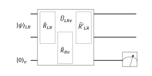
Figure 2: Quantum-circuit diagram of arbitrary combinations of depolarization and rotations. A quantum state $\left|\psi\right\rangle_{LR}$ and an auxiliary vacuum state evolve according to an SU(3) transformation $\hat{U}_{LRv}$, which contains all 7 degrees of freedom of a nondepolarizing Mueller matrix plus an additional phase. The entire circuit corresponds to the transformation (26) and transforms the Stokes vectors via a nondepolarizing Mueller matrix for arbitrary input states $\left|\psi\right\rangle_{LR}$. It can alternatively be decomposed into the product of three rotation operations as per Reck et al. (1994), with the first and last Euler angle of the middle rotation being the same de Guise et al. (2018).

The unitary operations described by (26) account for all deterministic Mueller matrices: arbitrary combinations of the three parameters of retarders and the four parameters of diattenuators. They can be recast into a Kraus operator representation of a quantum channel acting only on $\hat{\rho}$ of the form (18) with some minimum number of Kraus operators, such as through $\hat{K}_{l}=\left\langle l\right|_{v}\hat{U}_{LRv}\left|0\right\rangle_{v}$. While varying the number of Kraus operators represents some freedom in a description of the quantum channel, even the decomposition with the minimum number of Kraus operators is only unique up to unitary transformations $\hat{K}_{l^{\prime}}\to\sum_{n}u_{l^{\prime}l}\hat{K}_{l}$ for some unitary operator with matrix elements $u_{l^{\prime}l}$. We stress that this freedom underlies only the description of the quantum channel for the classical Mueller matrix; the effect of the quantum channel is always the same as that of (26). Because of this we conclude that all classical Mueller matrices that can be described by pure nondepolarizing operations correspond to photon-number-conserving quantum operations within a potentially-enlarged Hilbert space.

It is intriguing that the classical nondepolarizing degrees of freedom contained in $\mathbf{J}\in\text{SL}\left(2,\mathds{C}\right)$ are here recast into degrees of freedom of $\mathbf{U}_{LRv}\in\text{SU}(3)$. These groups certainly do not have the same structure, yet conspire to yield the same physical transformations. Our results show that any Jones matrix $\mathbf{J}$ acting on $\mathbf{E}$ can be represented as a truncated unitary matrix acting on a vector of creation operators $\left(\hat{a}^{\dagger}_{L},\hat{a}^{\dagger}_{R},\cdots\right)^{T}$ if the remaining modes begin in their vacuum states. This truncation always yields a complex $2\times 2$ matrix that can be rescaled to become an element of $\text{SL}(2,\mathds{C})$. Restricting to a single extra mode, such a truncation is equivalent to projecting from points on a hypersphere $S^{5}$ to points on $S^{3}$ Zyczkowski and Sommers (2000). These truncations have been studied from the point of view of random matrices, for which the distribution of points as well as the distribution of the eigenvalues of the truncated unitaries are known analytically Zyczkowski and Sommers (2000), and may be important for predicting the effect of a random nondepolarizing Mueller matrix.

II.3 Depolarizers and number-non-conserving operations

Seeing that number-conserving quantum operations parametrize the seven parameters of nondepolarizing Mueller matrices, the remaining nine free parameters of a general Mueller matrix must be described by quantum operations that do not conserve photon number in an enlarged Hilbert space. One must instead allow for unitary operations that change the total number of excitations in the larger space. As shown explicitly in Moyano-Fernández and Garcia-Escartin (2017), unitary transformations on a state allow one to generate a much larger set of transformations than unitary transformations on creation operators .

Quantum theories of depolarization have been studied Ramos (2005); do Nascimento and Ramos (2005); Ball and Banaszek (2005); Klimov et al. (2008); Réfrégier and Luis (2008); Klimov and Sánchez-Soto (2010); Rivas and Luis (2013). Depending on the desired properties, one can compose various dynamical equations that lead to depolarized quantum states. However, this depolarization is usually restricted to one or two of the degrees of freedom of Mueller matrices; we seek a quantum description that simultaneously encompasses all of the remaining degrees of freedom.

A typical example of a depolarization process is partial depolarization, whereby perfectly polarized light is transformed into light with degree of polarization $p$, with ideal depolarization corresponding to $p=0$:

$$\begin{pmatrix}\hat{S}_{0}\\ \hat{S}_{1}\\ \hat{S}_{2}\\ \hat{S}_{3}\end{pmatrix}\to\begin{pmatrix}1&0&0&0\\ 0&p&0&0\\ 0&0&p&0\\ 0&0&0&p\\ \end{pmatrix}\begin{pmatrix}\hat{S}_{0}\\ \hat{S}_{1}\\ \hat{S}_{2}\\ \hat{S}_{3}\end{pmatrix}.$$ (27)

This is normally described by a quantum channel $\hat{\rho}\to p\hat{\rho}+\left(1-p\right)\hat{\mathds{1}}/\mathcal{N}$ with normalization constant $\mathcal{N}=\text{Tr}(\hat{\mathds{1}})$ Nielsen and Chuang (2000). However, that transformation does not always yield $\hat{S}_{0}\to\hat{S}_{0}$, because the probability of $\hat{\rho}$ being in a particular photon-number subspace is not guaranteed to be the same as the probability of $\hat{\mathds{1}}$ being in that subspace. Knowing the weight $p_{N}$ of $\hat{\rho}$ in each subspace would allow for an appropriate transformation

$$\hat{\rho}\to p\hat{\rho}+\left(1-p\right)\sum_{N}p_{N}\frac{\hat{\mathds{1}}_{N}}{N+1},$$ (28)

but we seek transformations that are independent of the initial state.

One way of achieving (28) is through a continuum of Kraus operators:

$$\hat{\rho}\to\left(\sqrt{p}\hat{\mathds{1}}\right)\hat{\rho}\left(\sqrt{p}\hat{\mathds{1}}\right)^{\dagger}+\int\left(\sqrt{1-p}\hat{R}\right)\hat{\rho}\left(\sqrt{1-p}\hat{R}\right)^{\dagger}d\hat{R},$$ (29)

where the integrand contains a normalized Haar measure $d\hat{R}$ for the rotation operators. This physically corresponds to the effect of random SU(2) rotations Rivas and Luis (2013). The validity of this transformation can be immediately verified using the properties $\int\hat{R}\hat{S}_{0}\hat{R}^{\dagger}d\hat{R}=S_{0}$ and $\int\hat{R}\hat{S}_{i}\hat{R}^{\dagger}d\hat{R}=0$ for $i=1,2,3$. If we seek a unitary operation in an enlarged Hilbert space to describe (29), we require a continuum of orthonormal states $\left|\boldsymbol{\theta}\right\rangle_{v}$ to be populated without transferring any population from the initial system:

$$\hat{\rho}\otimes\hat{0}_{v}\to\hat{U}\hat{\rho}\otimes\hat{0}_{v}\hat{U}^{\dagger},\quad\hat{U}=\int\hat{R}_{LR}\left(\boldsymbol{\theta}\right)\otimes\left|\boldsymbol{\theta}\right\rangle\left\langle 0\right|_{v}d\boldsymbol{\theta}.$$ (30)

This is our first glimpse into the general feature that depolarization channels correspond to transformations that cannot be thought of as photon-number-conserving.

We next seek quantum descriptions of polarization maps described by (11). Since this type of depolarization does not act isotropically on the Stokes operators, perhaps an arbitrary depolarization matrix can be constructed by adding an appropriate weight function $f\left(\hat{R}\right)$ to the integrand in (29). It turns out that Mueller matrices $M_{d}$ with arbitrary $\mathbf{m}$ can indeed be constructed by a weighted integral of SU(2) operations if we allow for arbitrary $f$. However, the corresponding Kraus operators $\hat{K}_{l}\propto\hat{R}_{l}\equiv\hat{R}\left(\phi_{l},\theta_{l},\psi_{l}\right)$ need to incorporate the weight factor $\sqrt{f}$; this restricts $f$ to the set of positive-semidefinite functions, which are not sufficient for constructing all $\mathbf{m}$ while ensuring $\hat{S}_{0}\to\hat{S}_{0}$.

For example, take the rotation operation decomposed into the three Euler angles as per (16) and define the weight function $f\left(\phi,\theta,\psi;a,b,c,d,e,f,g,h,i,j\right)$:

$$f= \left[-4a\sin(\psi)\sin(\phi)+4b\sin(\psi)\cos(\phi)-\pi c\cos(\psi)\right.$$ (31)

$$\left.-4d\cos(\psi)\sin(\phi)+4e\cos(\psi)\cos(\phi)+\pi f\sin(\psi)\right.$$

$$\left.+\pi g\cos(\phi)+\pi h\sin(\phi)+2i\cos(\theta)+j\right]/4\pi^{3}.$$

If we evaluate the effect of the transformation $\int_{0}^{2\pi}d\phi\int_{0}^{\pi}d\theta\int_{0}^{2\pi}d\psi\,f\hat{R}\hat{\rho}\hat{R}^{\dagger}$ (in which the measure differs from the Haar measure by a factor of $\sin\theta$), we find the Mueller matrix

$$M=\begin{pmatrix}j&0&0&0\\ 0&a&b&c\\ 0&d&e&f\\ 0&g&h&i\\ \end{pmatrix},$$ (32)

which for $j=1$, $b=d$, $c=g$, $f=h$ describes a general depolarizer. However, $f$ is clearly negative for some values of its argument, meaning this does not describe a valid Kraus operator map.

In general there are quite a few weight functions that allow for arbitrary parameters $a$ through $i$, but finding ones that are normalized ($j=1$) without compromising the independence of the other parameters is challenging. Here, the requirement of a CPTP map enforces the same constraint as derived classically for Mueller matrices. We see that CPTP maps generating Mueller matrices with $M_{00}=1$ can be formed by positive combinations of SU(2) rotations. Correspondingly, the only classically valid Mueller matrices with $M_{00}=1$ are positive sums of nondepolarizing Mueller matrices that each have $M_{00}=1$ (e.g., Gamel and James (2011)); namely, linear combinations of rotation operations. This intimate connection strongly suggests a quantum-mechanical origin for the requirement that depolarizing Mueller matrices be formed from positive combinations of nondepolarizing Mueller matrices Cloude (1986); Gil (2000); Simon et al. (2010); Gamel and James (2011).

We have not shown that quantum operations corresponding to depolarizing Mueller matrices must be formed from convex combinations of quantum operations corresponding to nondepolarizing Mueller matrices. While a CPTP map that enacts a combination of SU(2) operations is a sufficient condition for generating Mueller matrices with $M_{00}=1$, it is by no means a necessary condition. For example, given that a set of Kraus operators $\left\{\hat{K}_{l}\right\}$ yields a valid depolarizing Mueller matrix, so too must the set of Kraus operators $\left\{\hat{K}_{l^{\prime}}\right\}$, where we can choose

$$\hat{K}_{l}=\sqrt{p_{l}}\hat{R}_{l},\quad\sum_{l}p_{l}=1$$ (33)

$$\hat{K}_{l^{\prime}}=\sum_{l}u_{l^{\prime}l}\hat{K}_{l},\quad\sum_{l^{\prime}}u_{l^{\prime}k}^{*}u_{l^{\prime}l}=\delta_{kl}.$$

Each individual transformation $\hat{K}_{l^{\prime}}\hat{\rho}\hat{K}_{l^{\prime}}^{\dagger}$ does not yield a Mueller matrix; in fact, the individual transformations of the Stokes operators no longer yield a linear combinations of Stokes operators. By no means does quantum mechanics mandate that a depolarizing Mueller matrix be described by a convex combination of processes corresponding to nondepolarizing Mueller matrices.

Still, we hypothesize that CPTP maps that send Stokes operators to linear combinations of Stokes operators always permit a decomposition into convex combinations of CPTP maps corresponding to nondepolarizing Mueller matrices. If we restrict our attention to maps that do not intermix the different photon-number subspaces, the results of Gamel and James (2011) immediately prove our hypothesis: since a map corresponding to a Mueller matrix must have the same behaviour on the Stokes operators regardless of the quantum state, one could work exclusively in the single-photon subspace, on which CPTP maps correspond exactly to the classical result of requiring convex combinations of nondepolarizing Mueller matrices. It is not far-fetched to believe that only those maps that do not intermix the different photon-number subspaces can send Stokes operators to linear combinations of Stokes operators. Validating this claim for general quantum operations will be the result of future work.

Convex combinations of the operations described in (26) are thus sufficient for describing all classical Mueller matrices. If the Kraus operators $\left\{\hat{K}_{l}^{(i)}\right\}_{l}$ correspond to Mueller matrix $M^{(i)}$, we have that the transformation

$$\mathcal{E}\left(\hat{\rho}\right)=\sum_{i}p_{i}\sum_{l}\hat{K}_{l}^{(i)}\hat{\rho}\hat{K}_{l}^{(i)\dagger}$$ (34)

corresponds to the Mueller matrix

$$M=\sum_{i}p_{i}M^{(i)}.$$ (35)

The new set of Kraus operators $\left\{\sqrt{p_{i}}\hat{K}_{l}^{(i)}\right\}_{l,i}$ is sufficient for describing $M$ quantum-mechanically. The freedom within the weights $p_{i}$, which need number no more than four Cloude (1986), provides the remaining degrees of freedom found in arbitrary Mueller matrices. This concludes our quest for determining quantum operations corresponding to all Mueller matrices.

II.3.1 Other descriptions of depolarizers

Quantum mechanics may provide more insight into other forms of depolarizing matrices. Since the lower-right $3\times 3$ submatrix of Mueller matrices representing depolarizers must be symmetric, the remaining three parameters describing arbitrary depolarization come as the vector $\mathbf{P}$ in

$$M_{d}=\begin{pmatrix}1&\mathbf{0}\\ \mathbf{P}^{T}&\mathbf{m}\end{pmatrix}.$$ (36)

There is no way that this can be construed as a positive sum of nondepolarizing Mueller matrices Gil (2000), but this form of depolarizers has indeed been used (e.g. Lu and Chipman (1996)). It is hard to conceive of quantum operations that take $\hat{S}_{i}\to\sum_{j=1}^{3}M_{ij}\hat{S}_{j}+M_{i0}\hat{S}_{0}$ for nonzero $M_{i0}$ that retain $\hat{S}_{0}\to\hat{S}_{0}$, and we will show an explicit example of where this difficulty lies.

One example of a process described by (36) is the operation that takes all incident light and converts it to light of a specific polarization [$\mathbf{m}=\textbf{0}$ and $\mathbf{P}=\left(0,0,1\right)$]. For left-circular polarization, this is the operation

$$\mathcal{E} \left(\hat{\rho}\right)=$$ (37)

$$\sum_{M=0}^{\infty}\sum_{m=0}^{M}\left|M,0\right\rangle\left\langle m,M-m\right|\hat{\rho}\sum_{N=0}^{\infty}\sum_{n=0}^{N}\left|n,N-n\right\rangle\left\langle N,0\right|,$$

where

$$\left|m,n\right\rangle\equiv\frac{\hat{a}^{\dagger}_{L}\vphantom{a}{}^{m}\hat{a}^{\dagger}_{R}\vphantom{a}{}^{n}}{\sqrt{m!n!}}\left|\text{vac}\right\rangle.$$ (38)

However, such a transformation is not trace-preserving, because the Kraus operators sum to $\sum_{N=0,m,n}\left|n,N-n\right\rangle\left\langle m,N-m\right|\neq\hat{\mathds{1}}$.

We can attempt to achieve a trace-preserving transformation by enacting

$$\mathcal{E}\left(\hat{\rho}\right)=\sum_{l=1}^{L}\left[\sum_{M=0}^{\infty}\left|M,0\right\rangle\left(\sum_{m=0}^{M}\left\langle m,M-m\right|\frac{\text{e}^{\text{i}\tfrac{2\pi lm}{L}}}{\sqrt{L}}\right)\right]\hat{\rho}\left[\sum_{N=0}^{\infty}\left(\sum_{n=0}^{N}\frac{\text{e}^{-\text{i}\tfrac{2\pi ln}{L}}}{\sqrt{L}}\left|n,N-n\right\rangle\right)\left\langle N,0\right|\right].$$ (39)

For a fixed maximum particle number $L-1$ this transformation indeed converts all incoming light into left-circularly-polarized light in a trace-preserving manner, due to the orthonormality condition

$$\frac{1}{L}\sum_{l=1}^{L}\text{e}^{\text{i}\tfrac{2\pi l\left(m-n\right)}{L}}=\delta_{mn},\quad\left|m-n\right|<L.$$ (40)

However, in order to generate a Mueller matrix transformation on the Stokes operators, this transformation must hold for arbitrarily large photon numbers. If we allow the formal limit $L\to\infty$, then the Kraus operators

$$\hat{K}_{l}=\sum_{M=0}^{\infty}\sum_{m=0}^{M}\left|M,0\right\rangle\left\langle m,M-m\right|\frac{\text{e}^{\text{i}\tfrac{2\pi lm}{L}}}{\sqrt{L}}$$ (41)

form a CPTP map corresponding to the Mueller matrix

$$M=\begin{pmatrix}1&0&0&0\\ 0&0&0&0\\ 0&0&0&0\\ 1&0&0&0\\ \end{pmatrix}.$$ (42)

The insight gained from quantum mechanics is that the Kraus operators in (41) are not physical. The true limit required is indeed $L\to\infty$, but requires maintaining $L\in\mathds{Z}$. While this bears resemblance to a discrete Fourier transform, the latter requires a substitution of $L\to M$ in (41). In the limit of $L\to\infty$, all of the Kraus operators vanish, obliterating the potential for achieving the desired CPTP map. We see that the trace-preservation condition of quantum mechanics negates the possibility of certain depolarization Mueller matrices being valid for all input states, which is typically an assumption of polarimetry. However, in realistic scenarios with a limited photon number, we see that certain “nonphysical” Mueller matrices become viable! This can help explain the validity of experimentally found Mueller matrices that seem to contradict known physical constraints (see, e.g., Simon et al. (2010)); perhaps the Mueller matrices found would not have been identical for other input states.

III Discussion and conclusions

The main feature of quantum polarimetry is that the quantum Stokes operators must transform according to Mueller calculus, regardless of the quantum state in question, for the former to agree with the predictions of classical polarimetry. A few simple quantum operations provide the building blocks for quantum polarimetry, and the degrees of freedom of an arbitrary Mueller matrix represent the various ways in which these building blocks can be combined.

One implication of the quantum channels described here is that all of polarimetry can be described in a trace-preserving manner. Total probability can always be conserved while explaining both deterministic and nondeterministic Mueller matrices, albeit with some information leaking to the environment about the states and transformations in question. The quantum channels can then be further decomposed into quantum master equations for the time evolution of systems evolving under nondepolarizing and depolarizing channels; and, conversely, it can immediately be seen whether a given quantum master equation corresponds to a classical Mueller-matrix transformation.

Another important result is the distinction between depolarizing and nondepolarizing processes, which has garnered much attention Gil and Bernabeu (1985); Simon (1987, 1990); Anderson and Barakat (1994); Cloude and Pottier (1995); Gil (2000); Zakeri et al. (2013). By assessing whether a process can be described by an operation that conserves photon number in an enlarged Hilbert space, one can immediately discern whether the associated Mueller matrix is nondepolarizing. All processes that require descriptions whereby modes in an enlarged Hilbert space are excited without de-exciting modes in the Hilbert space of $L$ and $R$ must be deemed depolarizing. We hope that this distinction proves useful in future studies of depolarization.

It is well-known that nondepolarizing Mueller matrices can be represented in the proper orthochronous Lorentz group Barakat (1981). However, there is no such constraint on the corresponding Kraus operators; the projections

$$\hat{K}_{l}=\left\langle l\right|_{v}\hat{U}_{LRv}\left|0\right\rangle_{v}=\left\langle 0\right|_{v}\hat{U}_{LRv}\left|0\right\rangle_{v}\frac{\left(\alpha_{1}\hat{a}_{L}+\alpha_{2}\hat{a}_{R}\right)^{l}}{\sqrt{l!}}$$ (43)

need not form a group ($\alpha_{1}$ and $\alpha_{2}$ are components of $\mathbf{U}_{LRv}$ as per Appendix A). For a $4\times 4$ Lorentz matrix $\Lambda$, we can find many decompositions

$$\sum_{l}\hat{K}_{l}^{\dagger}\hat{S}_{\mu}\hat{K}_{l}=\sum_{\nu}\Lambda_{\mu\nu}\hat{S}_{\nu},$$ (44)

and the Kraus operators conspire to yield a Lorentz transformation. We have shown that the classical degrees of freedom found in $\Lambda_{\mu\nu}$ correspond to the degrees of freedom in truncated unitary matrices acting on vectors of creation operators. Since this is equivalent to a $2\times 2$ complex matrix acting on $\left(\hat{a}^{\dagger}_{L},\hat{a}^{\dagger}_{R}\right)^{T}$, it is equivalent to a $2\times 2$ complex Jones matrix $\mathbf{J}$ acting on $\mathbf{E}$ with the same matrix elements (up to a change of basis from linear to circular coordinate systems), and Jones matrices can indeed represent the Lorentz group. One arena in which this equivalence can be exploited is in the study of the aggregate properties of random nondepolarizing Mueller matrices.

We have conjectured above that quantum channels are responsible for all Mueller matrices being expressible as positive sums of nondepolarizing Mueller matrices (Ref. Simon et al. (2010) has recently shown that only such sums are permissible for transformations of spatially-dependent Stokes operators). A subset of the conjecture is that all quantum channels that take $\hat{S}_{0}\to\hat{S}_{0}$ while taking the other Stokes operators to linear combinations of Stokes operators must be able to be expressed as positive sums of nondepolarizing channels. This is related to studies of SU(2)-covariant channels, which give conditions for quantum channels to commute with SU(2) operations Keyl and Werner (1999); Boileau et al. (2008); Gour and Spekkens (2008); Marvian Mashhad (2012); Streltsov et al. (2017); specifically, this is related to channels for which

$$\text{e}^{\text{i}\theta\hat{S}_{0}}\mathcal{E}\left(\rho\right)\text{e}^{-\text{i}\theta\hat{S}_{0}}=\mathcal{E}\left(\text{e}^{\text{i}\theta\hat{S}_{0}}\rho\text{e}^{-\text{i}\theta\hat{S}_{0}}\right),$$ (45)

which have interesting physical implications Morris et al. (2019). However, such channels imply not only $\hat{S}_{0}\to\hat{S}_{0}$ but also $\hat{S}_{0}^{n}\to\hat{S}_{0}^{n}$ for arbitrary integer $n$, which is a more stringent requirement than that of polarimetry. Inspection of the transformation

$$\frac{\hat{\mathds{1}}_{N}}{N+1}\to\frac{1}{2}\left(\frac{\hat{\mathds{1}}_{N-1}}{N}+\frac{\hat{\mathds{1}}_{N+1}}{N+2}\right),$$ (46)

for example, shows the preservation of expectation values of $\hat{S}_{0}$ but not $\hat{S}_{0}^{2}$. This requirement automatically prevents the intermixing of subspaces with different photon numbers, whereas we conjecture that the intermixing of subspaces is prevented automatically by only limiting the linear transformations of Stokes operators (we expect this to be intimately linked with no-cloning arguments Keyl and Werner (1999)). The connection to covariant channels may be an optimal starting point for proving our conjecture.

Polarimetry is concerned with measurement; the goal is to characterize the changes effected by an intervening medium on an arbitrary input state. Armed with a quantum description of polarimetry, we can now discuss quantum strategies for estimating the elements of a Mueller matrix. It is well-known that quantum parameter estimation offers dramatic enhancements over classical parameter estimation for particular input states (see Sidhu and Kok (2019)Liu et al. (2019) for thorough recent reviews). A necessary ingredient for finding such an enhancement is knowing how a transformed quantum state varies with the parameter being estimated. This is an important application of our work; by explicitly finding an expression

$$\hat{\rho}^{\prime}\left(\boldsymbol{\lambda}\right)=\mathcal{E}_{\boldsymbol{\lambda}}\left(\hat{\rho}\right)=\sum_{l}\hat{K}_{l}\left(\boldsymbol{\lambda}\right)\hat{\rho}\hat{K}_{l}^{\dagger}\left(\boldsymbol{\lambda}\right)$$ (47)

for the dependence of a transformed state $\hat{\rho}^{\prime}$ on a set of parameters $\boldsymbol{\lambda}$, we can investigate the states that are most sensitive to changes in the parameters being measured Ji et al. (2008). In the case of polarimetry, the parameters $\boldsymbol{\lambda}$ correspond to the 16 degrees of freedom of a Mueller matrix, and we can now ascertain how arbitrary quantum states vary with changes in Mueller matrix parameters. This can be used in the quantum Fisher information paradigm to search for states with the potential to be more sensitive to Mueller matrix parameters than classical polarization states without needing to specify a specific measurement scheme. For example, the usefulness of polarization-squeezed states in reducing fluctuations in parameter estimation can be investigated in vacuo Alodzhants et al. (1995); Alodjants et al. (1998); Korolkova et al. (2002), similar to the usefulness of quadrature-squeezed light in interferometry Caves (1981); Yurke et al. (1986); Dowling (1998).

Some relevant works have discussed quantum methods for simultaneously measuring a few degrees of freedom of a Mueller matrix. Estimating a single rotation parameter is akin to phase estimation, which has been considerably optimized Collaboration (2011), and estimating a single attenuation parameter can be equivalent to transmission measurements, for which all Fock states outperform classical states of light Adesso et al. (2009); Yoon et al. (2020). One study showed the tradeoff in measuring a single rotation angle around a known axis together with a single attenuation parameter Crowley et al. (2014), which can be cast into the product of Mueller matrices $M_{R}$ describing rotations around a known axis and $M_{D}$ describing isotropic diattenuation [(10) with $q=r$] . There, suitably-chosen quantum states offer enhanced sensitivities over classical measurements. More recently, quantum advantages have been for simultaneously measuring all three rotation parameters Goldberg and James (2018). The search for quantum states and quantum estimation strategies that offer such advantages in the simultaneous estimation of all 16 degrees of freedom of a Mueller matrix certainly merits future study.

Quantum channels allow for more sophisticated transformations than those described by Mueller matrices. This opens the door to new avenues of characterizing substances thought to be described by Mueller matrices, through an analysis of the nonlinear transformations of Stokes parameters enacted by a substance. The quantum polarimetry described here is a crucial building block for such analyses.

We have exhaustively shown how to describe classical polarimetry by transformations on quantum states. The components of Mueller matrices can now be directly related to the parameters of quantum channels, from which we ascertain the variety of quantum transformations of light that lead to the same classical measurement results. This underscores the importance of quantum polarization for improving classical measurements and better understanding the true nature of light.

Appendix A Explicit results

For the pure diattenuation described by (24) and Fig. 1 in the main text, one can write the corresponding transformation matrix $\mathbf{T}$:

$$\hat{U}_{D}^{\dagger}\begin{pmatrix}\hat{v}^{\dagger}_{1}\\ \hat{a}^{\dagger}_{L}\\ \hat{a}^{\dagger}_{R}\\ \hat{v}_{2}^{\dagger}\end{pmatrix}\hat{U}_{D}=\mathbf{T}\begin{pmatrix}\hat{v}^{\dagger}_{1}\\ \hat{a}^{\dagger}_{L}\\ \hat{a}^{\dagger}_{R}\\ \hat{v}_{2}^{\dagger}\end{pmatrix}.$$ (48)

This $\mathbf{T}$ matrix is given by:

$$\left(\begin{array}[]{cccc}\sqrt{q}&\text{e}^{-\frac{\text{i}\psi}{2}}\sqrt{1-q}\cos\left(\frac{\theta}{2}\right)&\text{e}^{\frac{\text{i}\psi}{2}}\sqrt{1-q}\sin\left(\frac{\theta}{2}\right)&0\\ -\text{e}^{\frac{\text{i}\psi}{2}}\sqrt{1-q}\cos\left(\frac{\theta}{2}\right)&\frac{1}{2}\left[\sqrt{q}+\sqrt{r}+\left(\sqrt{q}-\sqrt{r}\right)\cos\left(\theta\right)\right]&\frac{1}{2}\text{e}^{\text{i}\psi}\left(\sqrt{q}-\sqrt{r}\right)\sin\left(\theta\right)&-\text{e}^{\frac{\text{i}\psi}{2}}\sqrt{1-r}\sin\left(\frac{\theta}{2}\right)\\ -\text{e}^{-\frac{\text{i}\psi}{2}}\sqrt{1-q}\sin\left(\frac{\theta}{2}\right)&\frac{1}{2}\text{e}^{-\text{i}\psi}\left(\sqrt{q}-\sqrt{r}\right)\sin\left(\theta\right)&\frac{1}{2}\left[\sqrt{q}+\sqrt{r}+\left(\sqrt{r}-\sqrt{q}\right)\cos\left(\theta\right)\right]&\text{e}^{-\frac{\text{i}\psi}{2}}\sqrt{1-r}\cos\left(\frac{\theta}{2}\right)\\ 0&\text{e}^{-\frac{\text{i}\psi}{2}}\sqrt{1-r}\sin\left(\frac{\theta}{2}\right)&-\text{e}^{\frac{\text{i}\psi}{2}}\sqrt{1-r}\cos\left(\frac{\theta}{2}\right)&\sqrt{r}\\ \end{array}\right).$$ (49)

While $\mathbf{T}$ is unitary, its action on $\hat{a}^{\dagger}_{L}$ and $\hat{a}^{\dagger}_{R}$ after tracing out the two vacuum modes is not unitary, with the matrix in (25) corresponding only to the middle $2\times 2$ block of $\mathbf{T}$. The extra available degrees of freedom of the outer elements of $\mathbf{T}$ do not affect the polarimetric results. The Mueller matrix for this transformation is given by

$$M_{D}= \left(\begin{array}[]{cccc}\frac{q+r}{2}&\frac{1}{2}(q-r)\cos(\psi)\sin(\theta)\\ \frac{1}{2}(q-r)\cos(\psi)\sin(\theta)&\frac{1}{4}\left\{q+r+2\sqrt{qr}+\left[\cos^{2}(\theta)-\cos(2\psi)\sin^{2}(\theta)\right]\left(-q-r+2\sqrt{qr}\right)\right\}\\ \frac{1}{2}(q-r)\sin(\theta)\sin(\psi)&\frac{1}{4}\left(q+r-2\sqrt{qr}\right)\sin^{2}(\theta)\sin(2\psi)\\ \frac{1}{2}(q-r)\cos(\theta)&\frac{1}{4}\left(q+r-2\sqrt{qr}\right)\cos(\psi)\sin(2\theta)\\ \end{array}\right.$$ (50)

$$\left.\begin{array}[]{cccc}\frac{1}{2}(q-r)\sin(\theta)\sin(\psi)&\frac{1}{2}(q-r)\cos(\theta)\\ \frac{1}{4}\left(q+r-2\sqrt{qr}\right)\sin^{2}(\theta)\sin(2\psi)&\frac{1}{4}\left(q+r-2\sqrt{qr}\right)\cos(\psi)\sin(2\theta)\\ \frac{1}{4}\left\{q+r+2\sqrt{qr}+\left[\cos^{2}(\theta)+\cos(2\psi)\sin^{2}(\theta)\right]\left(-q-r+2\sqrt{qr}\right)\right\}&\frac{1}{4}\left(q+r-2\sqrt{qr}\right)\sin(2\theta)\sin(\psi)\\ \frac{1}{4}\left(q+r-2\sqrt{qr}\right)\sin(2\theta)\sin(\psi)&\frac{1}{4}\left[q+r+2\sqrt{qr}+\cos(2\theta)\left(q+r-2\sqrt{qr}\right)\right]\\ \end{array}\right).$$

For the SU(3) matrix $\mathbf{U}_{LRv}$ in (26) depicted schematically in Fig. 2 of the main text, we put the eight real degrees of freedom in the components $\alpha_{1}$, $\alpha_{2}$, $\beta_{1}$, and $\beta_{2}$:

$$\mathbf{U}_{LRv}=\begin{pmatrix}\alpha_{1}&\alpha_{2}&\sqrt{1-\left|\alpha_{1}\right|^{2}-\left|\alpha_{2}\right|^{2}}\text{e}^{\text{i}\theta_{a3}}\\ \beta_{1}&\beta_{2}&\sqrt{1-\left|\beta_{1}\right|^{2}-\left|\beta_{2}\right|^{2}}\text{e}^{\text{i}\theta_{b3}}\\ \sqrt{1-\left|\alpha_{1}\right|^{2}-\left|\beta_{1}\right|^{2}}\text{e}^{\text{i}\theta_{v1}}&\sqrt{1-\left|\alpha_{2}\right|^{2}-\left|\beta_{2}\right|^{2}}\text{e}^{\text{i}\theta_{v2}}&\sqrt{\left|\alpha_{1}\right|^{2}+\left|\beta_{1}\right|^{2}+\left|\alpha_{2}\right|^{2}+\left|\beta_{2}\right|^{2}-1}\text{e}^{\text{i}\theta_{v3}}\\ \end{pmatrix}.$$ (51)

The five angles are determined by the orthogonality equations between each pair of rows and columns, of which one is redundant; for example,

$$\alpha_{1}\beta_{1}^{*}+\alpha_{2}\beta_{2}^{*}+\sqrt{\left(1-\left|\alpha_{1}\right|^{2}-\left|\alpha_{2}\right|^{2}\right)\left(1-\left|\beta_{1}\right|^{2}-\left|\beta_{2}\right|^{2}\right)}\text{e}^{\text{i}\left(\theta_{a3}-\theta_{b3}\right)}=0.$$ (52)

There are no remaining degrees of freedom in this minimal description of a quantum channel corresponding to a nondepolarizing Mueller matrix.

References

- Bartholin (1670) E. Bartholin, Philosophical Transactions of the Royal Society of London: Giving Some Accounts of the Present Undertakings, Studies, and Labours, of the Ingenious, in Many Considerable Parts of the World 5, 2041 (1670).
- Stokes (1851) G. G. Stokes, Transactions of the Cambridge Philosophical Society 9, 399 (1851).
- Chandrasekhar (1950) S. Chandrasekhar, Radiative Transfer (Clarendon Press, 1950).
- Goldstein (2003) D. Goldstein, Polarized light (Dekker, Abingdon, 2003).
- Gil Pérez and Ossikovski (2016) J. J. G. Gil Pérez and R. Ossikovski, Polarized Light and the Mueller Matrix Approach (CRC Press, 2016).
- Azzam and Bashara (1977) R. M. A. Azzam and N. M. Bashara, Ellipsometry and polarized light (North-Holland Pub. Co., 1977).
- Collett (1992) E. Collett, Polarized light: fundamentals and applications (Marcel Dekker, Inc., 1992).
- Voss and Fry (1984) K. J. Voss and E. S. Fry, Appl. Opt. 23, 4427 (1984).
- Boulvert et al. (2004) F. Boulvert, B. Boulbry, G. L. Brun, B. L. Jeune, S. Rivet, and J. Cariou, Journal of Optics A: Pure and Applied Optics 7, 21 (2004).
- Ghosh et al. (2009) N. Ghosh, M. F. G. Wood, S.-h. Li, R. D. Weisel, B. C. Wilson, R.-K. Li, and I. A. Vitkin, Journal of Biophotonics 2, 145 (2009).
- Tuchin (2016) V. V. Tuchin, Journal of biomedical optics 21, 071114 (2016).
- Dulk et al. (1994) G. A. Dulk, Y. Leblanc, and A. Lecacheux, Astronomy and Astrophysics 286, 683 (1994).
- Tinbergen (2005) J. Tinbergen, Astronomical Polarimetry (Cambridge University Press, 2005).
- Born and Wolf (1999) M. Born and E. Wolf, Principles of optics: electromagnetic theory of propagation, interference and diffraction of light., 7th ed. (Cambridge University Press, 1999).
- Falkoff and MacDonald (1951) D. Falkoff and J. MacDonald, JOSA 41, 861 (1951).
- Aiello et al. (2007) A. Aiello, G. Puentes, and J. P. Woerdman, Phys. Rev. A 76, 032323 (2007).
- Galazo et al. (2018) R. Galazo, I. Bartolomé, L. Ares, and A. Luis, arXiv preprint arXiv:1811.12636 (2018).
- Beth (1935) R. A. Beth, Phys. Rev. 48, 471 (1935).
- Allen et al. (1992) L. Allen, M. W. Beijersbergen, R. J. C. Spreeuw, and J. P.. Woerdman, Physical Review A 45, 8185 (1992).
- Prakash and Chandra (1971) H. Prakash and N. Chandra, Phys. Rev. A 4, 796 (1971).
- Klyshko (1992) D. Klyshko, Physics Letters A 163, 349 (1992).
- Klyshko (1997) D. M. Klyshko, Journal of Experimental and Theoretical Physics 84, 1065 (1997).
- Tsegaye et al. (2000) T. Tsegaye, J. Söderholm, M. Atatüre, A. Trifonov, G. Björk, A. V. Sergienko, B. E. A. Saleh, and M. C. Teich, Phys. Rev. Lett. 85, 5013 (2000).
- Usachev et al. (2001) P. Usachev, J. Söderholm, G. Björk, and A. Trifonov, Optics Communications 193, 161 (2001).
- Bushev et al. (2001) P. A. Bushev, V. P. Karassiov, A. V. Masalov, and A. A. Putilin, Optics and Spectroscopy 91, 526 (2001).
- Luis (2002) A. Luis, Phys. Rev. A 66, 013806 (2002).
- Agarwal and Chaturvedi (2003) G. S. Agarwal and S. Chaturvedi, Journal of Modern Optics 50, 711 (2003), http://dx.doi.org/10.1080/09500340308235179 .
- Björk et al. (2015a) G. Björk, M. Grassl, P. de la Hoz, G. Leuchs, and L. L. Sánchez-Soto, Physica Scripta 90, 108008 (2015a).
- Luis and Donoso (2016) A. Luis and G. Donoso, Phys. Rev. A 94, 063858 (2016).
- Shabbir and Björk (2016) S. Shabbir and G. Björk, Phys. Rev. A 93, 052101 (2016).
- Goldberg and James (2017) A. Z. Goldberg and D. F. V. James, Phys. Rev. A 96, 053859 (2017).
- Bouchard et al. (2017) F. Bouchard, P. de la Hoz, G. Björk, R. Boyd, M. Grassl, Z. Hradil, E. Karimi, A. Klimov, G. Leuchs, J. Řeháček, and L. Sánchez-Soto, Optica 4, 1429 (2017).
- Goldberg and James (2018) A. Z. Goldberg and D. F. V. James, Physical Review A 98, 032113 (2018).
- Nielsen and Chuang (2000) M. A. Nielsen and I. L. Chuang, Quantum Computation and Quantum Information (Cambridge University Press, Cambridge, 2000).
- Mitchell et al. (2004) M. W. Mitchell, J. S. Lundeen, and A. M. Steinberg, Nature 429, 161 (2004).
- Gisin et al. (2002) N. Gisin, G. Ribordy, W. Tittel, and H. Zbinden, Rev. Mod. Phys. 74, 145 (2002).
- Tang et al. (2014) Z. Tang, Z. Liao, F. Xu, B. Qi, L. Qian, and H.-K. Lo, Phys. Rev. Lett. 112, 190503 (2014).
- Caves (1981) C. M. Caves, Phys. Rev. D 23, 1693 (1981).
- Helstrom (1967) C. Helstrom, Physics Letters A 25, 101 (1967).
- Helstrom (1973) C. W. Helstrom, International Journal of Theoretical Physics 8, 361 (1973).
- Holevo (1973) A. Holevo, Journal of Multivariate Analysis 3, 337 (1973).
- Holevo (1976) A. Holevo, in Proceedings of the Third Japan—USSR Symposium on Probability Theory (Springer, 1976) pp. 194–222.
- Giovannetti et al. (2004) V. Giovannetti, S. Lloyd, and L. Maccone, Science 306, 1330 (2004), http://science.sciencemag.org/content/306/5700/1330.full.pdf .
- Nagaoka (2005) H. Nagaoka, in Asymptotic Theory Of Quantum Statistical Inference: Selected Papers (2005) pp. 100–112.
- Paris (2009) M. G. A. Paris, International Journal of Quantum Information 07, 125 (2009).
- Tóth and Apellaniz (2014) G. Tóth and I. Apellaniz, Journal of Physics A: Mathematical and Theoretical 47, 424006 (2014).
- Demkowicz-Dobrzański et al. (2015) R. Demkowicz-Dobrzański, M. Jarzyna, and J. Kołodyński (Elsevier, 2015) pp. 345 – 435.
- Szczykulska et al. (2016) M. Szczykulska, T. Baumgratz, and A. Datta, Advances in Physics: X 1, 621 (2016).
- Sidhu and Kok (2019) J. S. Sidhu and P. Kok, arXiv preprint arXiv:1907.06628 (2019).
- Liu et al. (2019) J. Liu, H. Yuan, X.-M. Lu, and X. Wang, Journal of Physics A: Mathematical and Theoretical 53, 023001 (2019).
- Albarelli et al. (2020) F. Albarelli, M. Barbieri, M. Genoni, and I. Gianani, Physics Letters A , 126311 (2020).
- Altepeter et al. (2011) J. B. Altepeter, N. N. Oza, M. Medić, E. R. Jeffrey, and P. Kumar, Opt. Express 19, 26011 (2011).
- Yoon et al. (2020) S.-J. Yoon, J.-S. Lee, C. Rockstuhl, C. Lee, and K.-G. Lee, arXiv e-prints , arXiv:2001.06177 (2020), arXiv:2001.06177 [quant-ph] .
- Fry and Kattawar (1981) E. S. Fry and G. W. Kattawar, Appl. Opt. 20, 2811 (1981).
- Gil and Bernabeu (1985) J. J. Gil and E. Bernabeu, Optica Acta: International Journal of Optics 32, 259 (1985), https://doi.org/10.1080/713821732 .
- Cloude (1986) S. R. Cloude, Optik 75, 26 (1986).
- Barakat (1987) R. Barakat, Journal of Modern Optics 34, 1535 (1987), https://doi.org/10.1080/09500348714551471 .
- Cloude (1990) S. R. Cloude, “Conditions for the physical realisability of matrix operators in polarimetry,” (1990).
- Givens and Kostinski (1993) C. R. Givens and A. B. Kostinski, Journal of Modern Optics 40, 471 (1993).
- Nagirner (1993) D. Nagirner, Astronomy and Astrophysics 275, 318 (1993).
- van der Mee (1993) C. V. M. van der Mee, Journal of Mathematical Physics 34, 5072 (1993), https://doi.org/10.1063/1.530343 .
- Rao et al. (1998) A. V. G. Rao, K. S. Mallesh, and Sudha, Journal of Modern Optics 45, 955 (1998), https://doi.org/10.1080/09500349808230890 .
- Gil (2000) J. J. Gil, JOSA A 17, 328 (2000).
- van Zyl et al. (2011) J. J. van Zyl, M. Arii, and Y. Kim, IEEE Transactions on Geoscience and Remote Sensing 49, 3452 (2011).
- Gil et al. (2013) J. J. Gil, I. S. José, and R. Ossikovski, J. Opt. Soc. Am. A 30, 32 (2013).
- Zakeri et al. (2013) A. Zakeri, M. H. M. Baygi, and K. Madanipour, Appl. Opt. 52, 7859 (2013).
- Fano (1949) U. Fano, J. Opt. Soc. Am. 39, 859 (1949).
- Fano (1954) U. Fano, Phys. Rev. 93, 121 (1954).
- Jauch and Rohrlich (1955) J. M. Jauch and F. Rohrlich, The Theory of Photons and Electrons, Addison-Wesley series in advanced physics (Addison-Wesley, 1955).
- Simon (1987) R. Simon, Journal of Modern Optics 34, 569 (1987), https://doi.org/10.1080/09500348714550541 .
- Kim et al. (1987) K. Kim, L. Mandel, and E. Wolf, J. Opt. Soc. Am. A 4, 433 (1987).
- Simon et al. (2010) B. N. Simon, S. Simon, F. Gori, M. Santarsiero, R. Borghi, N. Mukunda, and R. Simon, Physical review letters 104, 023901 (2010).
- Gamel and James (2011) O. Gamel and D. F. V. James, Opt. Lett. 36, 2821 (2011).
- Sarsen and Valagiannopoulos (2019) A. Sarsen and C. Valagiannopoulos, Phys. Rev. B 99, 115304 (2019).
- Humphreys et al. (2013) P. C. Humphreys, M. Barbieri, A. Datta, and I. A. Walmsley, Phys. Rev. Lett. 111, 070403 (2013).
- Tsang et al. (2016) M. Tsang, R. Nair, and X.-M. Lu, Phys. Rev. X 6, 031033 (2016).
- Paúr et al. (2016) M. Paúr, B. Stoklasa, Z. Hradil, L. L. Sánchez-Soto, and J. Rehacek, Optica 3, 1144 (2016).
- Yang et al. (2016) F. Yang, A. Tashchilina, E. S. Moiseev, C. Simon, and A. I. Lvovsky, Optica 3, 1148 (2016).
- Tang et al. (2016) Z. S. Tang, K. Durak, and A. Ling, Opt. Express 24, 22004 (2016).
- Tham et al. (2017) W.-K. Tham, H. Ferretti, and A. M. Steinberg, Phys. Rev. Lett. 118, 070801 (2017).
- Řehaček et al. (2017) J. Řehaček, Z. Hradil, B. Stoklasa, M. Paúr, J. Grover, A. Krzic, and L. L. Sánchez-Soto, Phys. Rev. A 96, 062107 (2017).
- Chrostowski et al. (2017) A. Chrostowski, R. Demkowicz-Dobrzański, M. Jarzyna, and K. Banaszek, International Journal of Quantum Information 15, 1740005 (2017), https://doi.org/10.1142/S0219749917400056 .
- Parniak et al. (2018) M. Parniak, S. Borówka, K. Boroszko, W. Wasilewski, K. Banaszek, and R. Demkowicz-Dobrzański, Phys. Rev. Lett. 121, 250503 (2018).
- Wiener (1930) N. Wiener, Acta Mathematica 55, 117 (1930).
- Wolf (1959) E. Wolf, Il Nuovo Cimento (1955-1965) 13, 1165 (1959).
- Collett (1970) E. Collett, American Journal of Physics 38, 563 (1970), http://dx.doi.org/10.1119/1.1976407 .
- Atkins and Dobson (1971) P. W. Atkins and J. C. Dobson, Proceedings of the Royal Society of London A: Mathematical, Physical and Engineering Sciences 321, 321 (1971), http://rspa.royalsocietypublishing.org/content/321/1546/321.full.pdf .
- Luis (2016) A. Luis, Progress in Optics 61, 283 (2016).
- Alodjants and Arakelian (1999) A. P. Alodjants and S. M. Arakelian, Journal of Modern Optics 46, 475 (1999).
- Klimov et al. (2005) A. B. Klimov, L. L. Sánchez-Soto, E. C. Yustas, J. Söderholm, and G. Björk, Phys. Rev. A 72, 033813 (2005).
- Sánchez-Soto et al. (2006) L. L. Sánchez-Soto, J. Söderholm, E. C. Yustas, A. B. Klimov, and G. Björk, Journal of Physics: Conference Series 36, 177 (2006).
- Luis (2007a) A. Luis, Phys. Rev. A 75, 053806 (2007a).
- Luis (2007b) A. Luis, Optics Communications 273, 173 (2007b).
- Klimov et al. (2010) A. B. Klimov, G. Björk, J. Söderholm, L. S. Madsen, M. Lassen, U. L. Andersen, J. Heersink, R. Dong, C. Marquardt, G. Leuchs, and L. L. Sánchez-Soto, Phys. Rev. Lett. 105, 153602 (2010).
- Björk et al. (2010) G. Björk, J. Söderholm, L. L. Sánchez-Soto, A. B. Klimov, I. Ghiu, P. Marian, and T. A. Marian, Optics Communications 283, 4440 (2010), electromagnetic Coherence and Polarization.
- Björk et al. (2015b) G. Björk, A. B. Klimov, P. de la Hoz, M. Grassl, G. Leuchs, and L. L. Sánchez-Soto, Phys. Rev. A 92, 031801 (2015b).
- Hauge (1980) P. Hauge, Surface Science 96, 108 (1980).
- Layden et al. (2012) D. Layden, M. F. G. Wood, and I. A. Vitkin, Opt. Express 20, 20466 (2012).
- Azzam (1985) R. M. A. Azzam, Optica Acta: International Journal of Optics 32, 1407 (1985).
- Ling et al. (2006) A. Ling, K. P. Soh, A. Lamas-Linares, and C. Kurtsiefer, Phys. Rev. A 74, 022309 (2006).
- Simon (1990) R. Simon, Optics Communications 77, 349 (1990).
- Chipman (1995) R. A. Chipman, “Handbook of optics,” (McGraw-Hill, 1995) Chap. 22: Polarimetry, 2nd ed.
- Lu and Chipman (1996) S.-Y. Lu and R. A. Chipman, J. Opt. Soc. Am. A 13, 1106 (1996).
- Simon (1982) R. Simon, Optics Communications 42, 293 (1982).
- Varshalovich et al. (1988) D. A. Varshalovich, A. N. Moskalev, and V. K. Khersonskii, Quantum theory of angular momentum : irreducible tensors, spherical harmonics, vector coupling coefficients, 3nj symbols (World Scientific Pub, 1988).
- Leonhardt (2003) U. Leonhardt, Reports on Progress in Physics 66, 1207 (2003).
- Specht et al. (2009) H. P. Specht, J. Bochmann, M. Mücke, B. Weber, E. Figueroa, D. L. Moehring, and G. Rempe, Nature Photonics 3, 469 (2009).
- Beck et al. (2016) K. M. Beck, M. Hosseini, Y. Duan, and V. Vuletić, Proceedings of the National Academy of Sciences 113, 9740 (2016), https://www.pnas.org/content/113/35/9740.full.pdf .
- Reck et al. (1994) M. Reck, A. Zeilinger, H. J. Bernstein, and P. Bertani, Phys. Rev. Lett. 73, 58 (1994).
- Clements et al. (2016) W. R. Clements, P. C. Humphreys, B. J. Metcalf, W. S. Kolthammer, and I. A. Walmsley, Optica 3, 1460 (2016).
- de Guise et al. (2018) H. de Guise, O. Di Matteo, and L. L. Sánchez-Soto, Phys. Rev. A 97, 022328 (2018).
- Zyczkowski and Sommers (2000) K. Zyczkowski and H.-J. Sommers, Journal of Physics A: Mathematical and General 33, 2045 (2000).
- Moyano-Fernández and Garcia-Escartin (2017) J. J. Moyano-Fernández and J. C. Garcia-Escartin, Optics Communications 382, 237 (2017).
- Ramos (2005) R. V. Ramos, Journal of Modern Optics 52, 2093 (2005), https://doi.org/10.1080/09500340500147208 .
- do Nascimento and Ramos (2005) J. C. do Nascimento and R. V. Ramos, Microwave and Optical Technology Letters 47, 497 (2005), https://onlinelibrary.wiley.com/doi/pdf/10.1002/mop.21210 .
- Ball and Banaszek (2005) J. L. Ball and K. Banaszek, Open Systems & Information Dynamics 12, 121 (2005).
- Klimov et al. (2008) A. B. Klimov, J. L. Romero, L. L. Sánchez-Soto, A. Messina, and A. Napoli, Phys. Rev. A 77, 033853 (2008).
- Réfrégier and Luis (2008) P. Réfrégier and A. Luis, J. Opt. Soc. Am. A 25, 2749 (2008).
- Klimov and Sánchez-Soto (2010) A. B. Klimov and L. L. Sánchez-Soto, Physica Scripta T140, 014009 (2010).
- Rivas and Luis (2013) A. Rivas and A. Luis, Phys. Rev. A 88, 052120 (2013).
- Anderson and Barakat (1994) D. G. M. Anderson and R. Barakat, J. Opt. Soc. Am. A 11, 2305 (1994).
- Cloude and Pottier (1995) S. R. Cloude and E. Pottier, Optical Engineering 34, 1599 (1995).
- Barakat (1981) R. Barakat, Optics Communications 38, 159 (1981).
- Keyl and Werner (1999) M. Keyl and R. F. Werner, Journal of Mathematical Physics 40, 3283 (1999), https://doi.org/10.1063/1.532887 .
- Boileau et al. (2008) J.-C. Boileau, L. Sheridan, M. Laforest, and S. D. Bartlett, Journal of Mathematical Physics 49, 032105 (2008), https://doi.org/10.1063/1.2884583 .
- Gour and Spekkens (2008) G. Gour and R. W. Spekkens, New Journal of Physics 10, 033023 (2008).
- Marvian Mashhad (2012) I. Marvian Mashhad, Symmetry, Asymmetry and Quantum Information, Ph.D. thesis, University of Waterloo (2012).
- Streltsov et al. (2017) A. Streltsov, G. Adesso, and M. B. Plenio, Rev. Mod. Phys. 89, 041003 (2017).
- Morris et al. (2019) B. Morris, B. Yadin, M. Fadel, T. Zibold, P. Treutlein, and G. Adesso, arXiv e-prints , arXiv:1908.11735 (2019), arXiv:1908.11735 [quant-ph] .
- Ji et al. (2008) Z. Ji, G. Wang, R. Duan, Y. Feng, and M. Ying, IEEE Transactions on Information Theory 54, 5172 (2008).
- Alodzhants et al. (1995) A. Alodzhants, S. Arakelyan, and A. Chirkin, Journal of Experimental and Theoretical Physics 81, 34 (1995).
- Alodjants et al. (1998) A. Alodjants, S. Arakelian, and A. Chirkin, Applied Physics B: Lasers & Optics 66 (1998).
- Korolkova et al. (2002) N. Korolkova, G. Leuchs, R. Loudon, T. C. Ralph, and C. Silberhorn, Phys. Rev. A 65, 052306 (2002).
- Yurke et al. (1986) B. Yurke, S. L. McCall, and J. R. Klauder, Phys. Rev. A 33, 4033 (1986).
- Dowling (1998) J. P. Dowling, Phys. Rev. A 57, 4736 (1998).
- Collaboration (2011) The L.I.G.O. Scientific Collaboration, Nature Physics 7, 962 (2011).
- Adesso et al. (2009) G. Adesso, F. Dell’Anno, S. De Siena, F. Illuminati, and L. A. M. Souza, Phys. Rev. A 79, 040305 (2009).
- Crowley et al. (2014) P. J. D. Crowley, A. Datta, M. Barbieri, and I. A. Walmsley, Phys. Rev. A 89, 023845 (2014).