Theory and applications of parton pseudodistributions

Abstract

We review the basic theory of the parton pseudodistributions approach and its applications to lattice extractions of parton distribution functions. The crucial idea of the approach is the realization that the correlator $M(z,p)$ of the parton fields is a function ${\cal M}(\nu,-z^{2})$ of Lorentz invariants $\nu=-(zp)$, the Ioffe time, and the invariant interval $z^{2}$. This observation allows to extract the Ioffe-time distribution ${\cal M}(\nu,-z^{2})$ from Euclidean separations $z$ accessible on the lattice. Another basic feature is the use of the ratio ${\mathfrak{M}}(\nu,-z^{2})\equiv{\cal M}(\nu,-z^{2})/{\cal M}(0,-z^{2})$, that allows to eliminate artificial ultraviolet divergence generated by the gauge link for space-like intervals. The remaining $z^{2}$-dependence of the reduced Ioffe-time distribution ${\mathfrak{M}}(\nu,-z^{2})$ corresponds to perturbative evolution, and can be converted into the scale-dependence of parton distributions $f(x,\mu^{2})$ using matching relations. The $\nu$-dependence of ${\mathfrak{M}}(\nu,-z^{2})$ governs the $x$-dependence of parton densities $f(x,\mu^{2})$. The perturbative evolution was successfully observed in exploratory quenched lattice calculation. The analysis of its precise data provides a framework for extraction of parton densities using the pseudodistributions approach. It was used in the recently performed calculations of the nucleon and pion valence quark distributions. We also discuss matching conditions for the pion distribution amplitude and generalized parton distributions, the lattice studies of which are now in progress.

PACS numbers:12.38.-t, 11.15.Ha, 12.38.Gc

1 Introduction: Why pseudo-PDFs?

Feynman’s parton distribution functions[1] (PDFs) $f(x)$ are the basic building blocks for the description of hard inclusive processes in quantum chromodynamics (QCD). Generically, they are defined through matrix elements of bilocal operators of the $\langle p|\phi(0)\phi(z)|p\rangle\equiv M(z,p)$ type taken on the light cone $z^{2}=0$.

Since PDFs accumulate nonperturbative information about the hadron structure, they are a natural candidate for a lattice study. However, the intervals, that are strictly on the light cone, are not accessible on Euclidean lattices. Still, it is possible to perform lattice simulations for small space-like $z^{2}$, and to arrange then some method of reaching the $z^{2}=0$ limit.

The starting idea is to take the equal-time interval $z=\{0,0,0,z_{3}\}$. It was put forward in Refs. [2, 3] and emphasized by X. Ji in the paper [4] that strongly stimulated further development in the lattice studies of the PDFs (see Ref. [5] for a recent review and references). Other objects for a lattice investigation include the pion distribution amplitude[6] (DA), a function playing a fundamental role in perturbative QCD studies of hard exclusive processes, and generalized parton distributions[7, 8, 9].

By Lorentz invariance, the matrix element $M(z,p)$ is a function of the Ioffe time[10] $(pz)\equiv-\nu$ and of the interval $z^{2}$. Writing it as a function of these invariants, $M(z,p)\equiv{\cal M}(\nu,-z^{2})$, one deals with the Ioffe-time pseudodistribution[11] ${\cal M}(\nu,-z^{2})$, which is a generalization of the light-cone Ioffe-time distribution[12] (ITD) ${\cal I}(\nu,\mu^{2})$ onto space-like intervals $z^{2}$. By definition, ${\cal I}(\nu,\mu^{2})$ is a Fourier transform of the light-cone PDF $f(x,\mu^{2})$, with the Ioffe time $\nu$ being the variable that is Fourier-conjugate to the parton momentum fraction variable $x$.

Analogously, taking the Fourier transform in $\nu$ of the pseudo-ITD ${\cal M}(\nu,-z^{2})$ gives the pseudo-PDF[11] ${\cal P}(x,-z^{2})$. By construction, ${\cal P}(x,-z^{2})$ is a Lorentz-covariant function, just like ${\cal M}(\nu,-z^{2})$. This means that the “$x$” variable is also Lorentz-invariant. It does not depend on a specific frame choice. In particular, there is no need to take an infinite momentum frame to define it. It can be shown[13, 14] that, for any contributing Feynman diagram, ${\cal P}(x,-z^{2})$ has the same support $-1\leq x\leq 1$ as the light-cone PDFs $f(x,\mu^{2})$ do, even though $z^{2}$ is space-like.

Hence, the pseudo-PDF ${\cal P}(x,z_{3}^{2})$ is the most natural generalization of the light-cone PDF $f(x,\mu^{2})$ onto space-like intervals. For $f(x,\mu^{2})$, the usual interpretation of the scale $\mu$ is that $1/\mu$ characterizes the distances at which the hadron structure is probed. In this sense, when one takes $z=\{0,0,0,z_{3}\}$, the scale $z_{3}$ in ${\cal P}(x,z_{3}^{2})$ is literally the distance at which the hadron structure is probed.

Thus, the $z_{3}$-dependence of the pseudo-ITD ${\cal M}(\nu=z_{3}p_{3},z_{3}^{2})$ comes in two ways. First, the $z_{3}$-dependence may be accompanied by the $p_{3}$-dependence: it comes through the product $z_{3}p_{3}=\nu$. The $\nu$-dependence of ${\cal M}(\nu,z_{3}^{2})$ converts into the $x$-dependence of ${\cal P}(x,z_{3}^{2})$ . The remaining $z_{3}^{2}$-dependence of ${\cal M}(\nu,z_{3}^{2})$ specifies how the $x$-shape of ${\cal P}(x,z_{3}^{2})$ changes with the change of the probing distance $z_{3}$.

In fact, the dependence on the probing distance may be interpreted in terms of the distribution of the parton’s transverse momentum[11]. Recall, that $\nu$ and $z^{2}$ are Lorentz invariants. Therefore, the pseudo-ITD ${\cal M}(\nu,-z^{2})$ is the same universal function of them, no matter how $\nu$ and $z^{2}$ were obtained from specific choices of $z$ and $p$. In particular, taking $z$ on the light front, $z=\{z_{+}=0,z_{-},z_{\perp}\}$, and a longitudinal $p=\{p_{+},p_{-},0_{\perp}\}$ gives ${\cal M}(\nu,z_{\perp}^{2})$, where $\nu=-p_{+}z_{-}$. In this situation, the $\nu$-dependence of ${\cal M}(\nu,z_{\perp}^{2})$ determines the $x$-distribution of the longitudinal “plus”-component of the parton momentum, while its $z_{\perp}^{2}$-dependence determines the distribution of its transverse momentum $k_{\perp}$.

Hence, the two arguments of the pseudo-ITD ${\cal M}(\nu,-z^{2})$ correspond to two different physical phenomena. Its dependence on the Ioffe time $\nu$ converts into the $x$-dependence of the pseudo-PDF ${\cal P}(x,-z^{2})$, which characterizes how the parton momentum increases with the increase of the hadron momentum. On the other hand, the dependence on $z^{2}$ characterizes a distribution of that part of the parton momentum that does not depend on the hadron momentum, so it may be connected with a “primordial” parton momentum distribution in the hadron rest frame[11].

In Ref. [4], it was proposed to convert the matrix element $M(z_{3},p)$ into the quasi-PDF $Q(y,p_{3})$. This is achieved by taking the Fourier transform of ${\cal M}(z_{3}p_{3},z_{3}^{2})$ with respect to $z_{3}$. The resulting function $Q(y,p_{3})$ characterizes the fraction $y$ of the third component of the hadron momentum $p_{3}$ carried by the parton. This fraction may take any value, from $-\infty$ to $\infty$, there is no restriction on it.

Since $z_{3}$ enters both in $\nu$ and $z_{3}^{2}$, the $y$-shape of $Q(y,p_{3})$ is governed both by the $\nu$-dependence of the pseudo-ITD ${\cal M}(\nu,z_{3}^{2})$ and by its $z_{3}^{2}$-dependence. Thus, the two different physical phenomena reflected in the $\nu$- and $z_{3}^{2}$-dependences of ${\cal M}(\nu,z_{3}^{2})$ are mixed in $Q(y,p_{3})$. Writing $z_{3}$ as $\nu/p_{3}$, one can convert the $z_{3}$-integral of ${\cal M}(z_{3}p_{3},z_{3}^{2})$ into the $\nu$-integral of ${\cal M}(\nu,\nu^{2}/p_{3}^{2})$. For large $p_{3}$, the second argument tends to zero, and one essentially deals with the $\nu$-integral of ${\cal M}(\nu,0)$, which gives the light-cone PDF $f(x)$. In other words, the $y$-shape of $Q(y,p_{3})$ depends on $p_{3}$, and reaches the PDF limit $f(y)$ when $p_{3}\to\infty$, i.e. in the infinite momentum frame. Taking the large-$p_{3}$ limit for $Q(y,p_{3})$ is the main idea[15] of the quasi-PDF approach.

To have a large momentum is always a challenge for a lattice simulation. Thus, the question is to which extent the efforts to get a large $p_{3}$ are justified. If the reason is to get a small value for the second argument of ${\cal M}(\nu,\nu^{2}/p_{3}^{2})$, then this can be achieved by simply taking a small $z_{3}$. And one can take then any value of $p_{3}$, from zero to the achievable maximum. For instance, in the lattice study performed in Ref. [17], there were 7 values of $p_{3}=p(2\pi/L)$, with $0\leq p\leq 6$. In other words, for each value of $z_{3}$, there were 7 values of the Ioffe-time parameter $\nu$, instead of just one value of $\nu$ obtained in a measurement for the largest achievable $p_{3}$. As we discussed, it is the $\nu$-dependence of ${\cal M}(\nu,z_{3}^{2})$ that determines the $x$-dependence of PDFs, and the pseudo-PDF approach allows to get a detailed information about it.

In this connection, we want to mention that another approach, the good lattice cross-sections, that was proposed and developed in Refs. [18, 19], is also based on the factorization in the coordinate space and the analysis of the Ioffe-time dependence.

In the present paper, we review the basic ideas of the pseudo-PDF approach formulated in Refs. [11, 20], further developed in Refs. [21, 22, 23, 24, 25, 26] and used in lattice analyses of Refs. [17, 27, 28].

In Sec. 2, we discuss the general aspects of the PDF concept. We start by illustrating the parton idea by using the simplest example of the handbag diagram for a scalar analog of deep inelastic scattering, and continue by outlining modifications necessary in a theory with spin-1/2 quarks and gauge fields. We describe the Ioffe-time distributions and the ratio method that is a very essential element of the pseudo-PDF approach. It allows, in particular, to efficiently get rid of the link-related ultraviolet divergences that are artifacts of using space-like field correlators. We also discuss in this section some general properties of the quasi-PDFs, in particular, their relation to the transverse-momentum dependence of parton distributions. We show that such a dependence described a “TMD” ${\cal F}(x,k_{p}erp^{2})$ is determined by the $z^{2}$-dependence of the pseudo-ITD ${\cal M}(\nu,-z^{2})$.

In Sec. 3, we investigate the nonperturbative aspects of the $P$-dependence of quasi-PDFs using some simple models for the TMD ${\cal F}(x,k_{p}erp^{2})$. We describe the main features of the nonperturbative evolution of the quasi-PDFs, in particular, the rate of approach of quasi-PDFs $Q(y,P)$ to their $P\to\infty$ limit that give the light-cone PDFs. We discuss the role of target-mass corrections $\sim(M^{2}/P^{2})^{n}$, and argue that they are actually much smaller than the $\sim(\langle k_{\perp}^{2}\rangle/P^{2})^{n}$ transverse-momentum corrections.

In Sec. 4, we give a discussion of the perturbative structure of the ITDs at one-loop level, concentrating both on the link-related ultraviolet divergences and on the infrared aspects connected with the perturbative evolution. A special attention is given to matching relations that allow to convert the $z_{3}^{2}$-dependence of the reduced ITD into the $\mu^{2}$-dependence of the light-cone PDFs.

In the next two sections, we discuss the results of lattice calculations[17, 27] guided by the pseudo-PDF approach ideas. We concentrate on applications of the pseudo-PDF approach concepts, skipping the questions related to actual lattice extraction of the data, the analysis of discretization errors, finite-volume effects, etc.

The results of the exploratory lattice study[17] based on the pseudo-PDF approach are described in Sec. 5. The high statistical accuracy of its data allows to perform a lattice study of perturbative evolution, the phenomenon that no other lattice simulations were able to detect yet. The analysis of the quenched data forms a basis for future studies of the perturbative evolution within lattice setups that are closer to the real-world QCD.

The results of a recent calculation[27] with dynamical fermions are discussed in Sec. 6. The PDFs extracted in this study are in much better agreement with phenomenological studies. However, larger statistical errors of the data do not allow to detect perturbative evolution.

In Sec. 7, we describe the derivation of matching relations for the pion distribution amplitude and generalized parton distributions that are necessary in the ongoing and future efforts for extraction of these distributions from the lattice.

Sec. 8 contains the summary of the paper.

The derivation of the spectral property $|x|\leq 1$ for the pseudo-PDFs is outlined in the Appendix.

2 Parton distributions

2.1 Handbag diagram and pseudo-PDFs

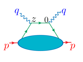
Figure 1: General handbag diagram for a virtual forward Compton amplitude in coordinate representation.

Historically, parton distributions were introduced to describe deep inelastic scattering (DIS). The usual starting point of DIS analysis is the forward Compton amplitude $T(q,p)$ which, in the lowest approximation, is given by a handbag diagram (see Fig. 1). To skip inessential complications related to spin (they do not affect the very concept of parton distributions and may be included when needed), we start with a simple example of a scalar handbag diagram, and write it in the coordinate representation

$$T(q,p)=\int{\differential^{4}z}\,e^{-i(qz)}\,D(z)\,\langle p|\phi(0)\phi(z)|p\rangle\ ,$$ (2.1)

where $D(z)=-i/4\pi^{2}z^{2}$ is the scalar massless propagator, $p$ is the target momentum and $q$ is the momentum of the hard probe.

The matrix element $\langle p|\phi(0)\phi(z)|p\rangle\equiv M(z,p)$ accumulates information about the target. To proceed with the $\differential^{4}z$ integral, one needs to know something about the dependence of $M(z,p)$ on the coordinate $z$.

It can be shown [14, 13] that, for each of contributing Feynman diagrams, $M(z,p)$ has the following representation (see Appendix A for some details)

$${M}(z,p) =\int_{-1}^{1}\differential x\,e^{-ix(pz)}\,{\cal P}(x,-z^{2})\ ,$$ (2.2)

where ${\cal P}(x,-z^{2})$ is the parton pseudodistribution function or pseudo-PDF, introduced in Ref. [11]. In the simplest case, when ${\cal P}(x,-z^{2})$ has no $z^{2}$-dependence, so that ${\cal P}(x,-z^{2})=f(x)$, the $\differential^{4}z$ integral becomes trivial, and we get

$$T_{0}(q,p)=-\int_{-1}^{1}\differential x\,\frac{f(x)}{(q+xp)^{2}+i\epsilon}\ ,$$ (2.3)

which is the well-known parton-model expression for the forward Compton amplitude, with $f(x)$ being the parton distribution function (PDF).

Note that Eq. (2.2) introduces the momentum fraction variable $x$ in an absolutely covariant way. One has no need to assume that $z^{2}=0$ or $p^{2}=0$ or to take an infinite momentum frame, etc., to define $x$. Of course, since the representation (2.2) works in general case, it also works if we take $z$ on the light cone. In particular, taking $z$ that has the light-cone “minus” component $z_{-}$ only, gives the representation

$$\langle p|\phi(0)\phi(z_{-})|p\rangle=\int_{-1}^{1}\differential x\,{\cal P}(x,0)\,e^{-ixp_{+}z_{-}}\,\ ,$$ (2.4)

which has the standard interpretation that $x$ is the fraction of the light-cone “plus” component $p_{+}$ of the target momentum carried by the parton.

However, we want to emphasize that $p$ in Eq. (2.3) is the actual hadron momentum satisfying $p^{2}=M^{2}$. In particular, writing

$$(q+xp)^{2}=2(qp)(x-x_{\rm Bj})+x^{2}M^{2}$$ (2.5)

(with $x_{\rm Bj}=-q^{2}/2(pq)$ is the Bjorken variable), and taking the imaginary part, we get the $\xi$-scaling expression [29, 30] for the relevant structure function

$$W_{0}(q,p)= \int_{0}^{1}dx\,f(x)\ \delta[2(qp)(x-x_{\rm Bj})+x^{2}M^{2}]=\frac{f(\xi_{\rm N})}{2(pq)\sqrt{1+\frac{4x_{\rm Bj}^{2}M^{2}}{Q^{2}}}}\ ,$$ (2.6)

where $Q^{2}=-q^{2}$ and $\xi_{N}$ is the Nachtmann variable[29]

$$\xi_{N}=\frac{2x_{\rm Bj}}{1+\sqrt{1+{4x_{\rm Bj}^{2}M^{2}}/{Q^{2}}}}\ .$$ (2.7)

Thus, Eq. (2.6) allows to calculate target-mass corrections.

On dimensional grounds, one may expect that further terms in the formal $z^{2}$-expansion ${\cal P}(x,-z^{2})=f(x)+z^{2}f_{4}(x)\ +\ldots+(z^{2})^{n}f_{2(n+1)}(x)+\ldots$ will be accompanied by extra $(1/Q^{2})^{n}$ factors, i.e. that such “higher twist” contributions to $T(q,p)$ are suppressed by powers of $1/Q^{2}$ for large $Q^{2}$. However, the light-cone singularity of the massless scalar propagator (which is $D(z)\sim 1/z^{2}$) is canceled by the $z^{2}$ factors, resulting in contributions containing $\delta^{4}(q+xp)$ and its derivatives. In DIS, $q$ is not proportional to $p$, and such contributions are treated as zero.

Thus, if ${\cal P}(x,-z^{2})$ is analytic on the light cone, the scalar handbag diagram is given by the twist-2 part alone. For spin-1/2 partons, the propagator $S^{c}(z)\sim\not{z}/(z^{2})^{2}$ is more singular, and the handbag diagram contains twist-2 and twist-4 terms. The twist-2 part is given by $\xi$-scaling expressions [29, 30] involving the twist-2 PDF $f(x)$, while the twist-4 part requires an independent function related to $\bar{\psi}D^{2}\psi$-type operators.

2.2 Light-cone singularities and factorization

One cannot use a formal $z^{2}$-expansion if ${\cal P}(x,-z^{2})$ is singular for $z^{2}=0$. In QCD and other renormalizable theories, ${\cal P}(x,-z^{2})$ has $\sim\ln(-z^{2})$ terms. These singularities are perfectly integrable when embedded in the expression (2.1) for $T(q,p)$: they just produce logarithmic $\ln(-q^{2})$ contributions that violate a strict dimensional scaling present in $T_{0}(q,p)$.

On the other hand, taking $z^{2}=0$ in the pseudo-PDFs themselves produces ultraviolet divergences in the perturbative expressions for matrix elements of $\phi(0)\phi(z)$ operators. Introducing some UV cut-off $\Lambda$ converts $\ln(-1/z^{2})$ into $\ln\Lambda^{2}$, and the resulting PDFs depend on the cut-off scale, $f(x)\to f(x,\Lambda^{2})$. The usual procedure is to use the dimensional regularization (DR) for momentum integrals $\differential^{4}k\to(\mu^{2})^{\epsilon}\differential^{4-2\epsilon}k$. After subtraction of the $1/\epsilon$ poles, one gets PDFs depending on the DR renormalization scale $\mu$. For the minimal $\overline{\rm MS}$ subtraction, one obtains the standard $\overline{\rm MS}$ parton densities $f(x)\to f(x,\mu^{2})$.

It should be emphasized that, if one keeps $z^{2}$ spacelike, then ${\cal P}(x,-z^{2})$ is finite, and no regularization for the $\ln(-z^{2})$ terms is needed. In this sense, the interval $z^{2}$ serves as an UV cut-off, and one may treat ${\cal P}(x,-z^{2})$ as just another type of a PDF, that is defined in a peculiar “$z^{2}$”-scheme rather in the $\overline{\rm MS}$ scheme. In fact, the PDFs of this $z^{2}$-scheme are more physical than the $\overline{\rm MS}$ ones. One may say that they literally measure the hadron structure at distances $d=\sqrt{-z^{2}}$.

However, the established standard is to use the $\overline{\rm MS}$-scheme PDFs $f(x,\mu^{2})$. In the expression for $T(q,p)$, written in terms of the momentum invariants $q^{2}=-Q^{2}$ and $x_{\rm B}=Q^{2}/2(pq)$, they appear through the factorization formula

$$T(x_{\rm B},Q^{2}) =\int_{-1}^{1}\frac{\differential x}{|x|}\,t(x_{\rm B}/x,Q^{2}/\mu^{2})\,f(x,\mu^{2})\ +\ {\rm higher\ twists}\,\ ,$$ (2.8)

in which the scaling-violating $\ln Q^{2}$ terms are split into the “short-distance” part $\ln Q^{2}/\mu^{2}$ present in the coefficient function $t(x_{\rm B}/x,Q^{2}/\mu^{2})$ and the evolution logarithms $\ln\mu^{2}$ present in the scale-dependent PDF $f(x,\mu^{2})$. This formula is obtained by applying the operator product expansion (OPE) to $T(q,p)$ written as

$$T(q,p)=\int{\differential^{4}z}\,e^{-i(qz)}\,\langle p|j(0)j(z)|p\rangle\ ,$$ (2.9)

i.e., in terms of the probing currents $j(0)$, $j(z)$. Similarly, one can apply the OPE to the product of fields $\phi(0)\phi(z)$ defining the pseudo-PDF. In non-gauge theories,

$${\cal P}(x,-z^{2})= \int_{-1}^{1}\frac{\differential w}{w}\,C(w,z^{2}\mu^{2})\,f(x/w,\mu^{2})+{\cal O}(z^{2})\ .$$ (2.10)

In this expression, the $\ln(-z^{2})$ terms are split between the coefficient function $C(w,z^{2}\mu^{2})$ and the PDF $f(x/w,\mu^{2})$. Here we write the factorization relation in the form following from the nonlocal light-cone OPE [31, 32] (see also Ref. [21]).

2.3 Gauge theories

In QCD, the quarks have spin 1/2, and the handbag diagram for the Compton amplitude is given by

$$T^{\mu\nu}(q,p)=\int{d^{4}z}\,e^{-i(qz)}\langle p|\bar{\psi}(0) \gamma^{\nu}\,S^{c}(-z)\,\gamma^{\mu}\,\psi(z)|p\rangle\ ,$$ (2.11)

where $S^{c}(z)=\not{z}/2\pi^{2}(z^{2})^{2}$ is the propagator for a massless fermion. Writing $\gamma^{\nu}\,\not{z}\,\gamma^{\mu}$ as $\left[g^{\nu\beta}g^{\mu\alpha}+g^{\nu\beta}g^{\mu\alpha}-g^{\mu\nu}g^{\alpha\beta}+i\epsilon^{\mu\nu\alpha\beta}\gamma_{5}\right]z_{\beta}\gamma_{\alpha}$ we get matrix elements $\langle p|\bar{\psi}(0)\,\gamma_{\alpha}\,\psi(z)|p\rangle$ and $\langle p|\bar{\psi}(0)\,\gamma_{5}\gamma_{\alpha}\,\psi(z)|p\rangle$ corresponding to unpolarized and polarized PDFs, respectively.

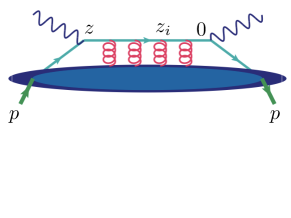
Figure 2: Structure of QCD factorization for DIS in covariant gauges.

Furthermore, in gauge theories, the handbag contribution in covariant gauges should be complemented by diagrams corresponding to operators $\bar{\psi}(0)\ldots\not{A}(z_{i})\ldots\psi(z)$ containing twist-0 gluonic field $A_{\mu_{i}}(z_{i})$ inserted into the fermion line between the points $z$ and $0$ (see Fig. 2). The sum of gluon insertions is equivalent to substituting the free propagator $S^{c}(z_{1}-z_{2})$ by a propagator ${\cal S}^{c}(z_{1},z_{2};A)$ of a quark in an external gluonic field $A$. This propagator satisfies the Dirac equation

$$i\left[\frac{\not{\partial}}{\partial z_{1}}-ig\not{A}(z_{1})\right]{\cal S}^{c}(z_{1},z_{2};A)=-\delta^{4}(z_{1}-z_{2})\ .$$ (2.12)

The solution of this equation may be written in the form

$${\cal S}^{c}(z_{1},z_{2};A)=E(z_{1},z_{2};A){\mathfrak{S}}^{c}_{\rm FS}(z_{1},z_{2};A)$$ (2.13)

involving the straight-line exponential

$${E}(z_{1},z_{2};A)\equiv P\exp{\left[ig\,\int_{0}^{1}dt\,(z_{2}^{\alpha}-z_{1}^{\alpha})\,A_{\alpha}((1-t)z_{1}+tz_{2})\right]}\ .$$ (2.14)

In its turn, the factor ${\mathfrak{S}}^{c}_{\rm FS}$ satisfies the Dirac equation (2.12) with the general vector potential $A^{\mu}(z)$ substituted [33, 34, 35] by the vector potential ${\mathfrak{A}}^{\mu}(z;z_{1})$ in the Fock-Schwinger (FS) gauge [36, 37] $(z-z_{1})_{\mu}{\mathfrak{A}}^{\mu}(z,z_{1})=0\ .$ It is given by

$${\mathfrak{A}}^{\mu}(z;z_{1})=(z-z_{1})_{\nu}\int_{0}^{1}\,\differential s\,s\,G^{\mu\nu}(z_{1}+s(z-z_{1}))\,.$$ (2.15)

Here, $z$ denotes the location of the field, while $z_{1}$ specifies the “fixed point” of the FS gauge, and in our case refers to an end-point in the Compton amplitude. Since the field-strength tensor $G^{\mu\nu}$ has twist equal to (at least) 1, the insertion of this field into the free propagator results in power $(\Lambda^{2}/Q^{2})^{l}$ corrections to the Compton amplitude. Thus, we can write

$${\cal S}^{c}(0,z;A)=E(0,z;A){S}_{c}(z)+{\rm higher\ twists}\ .$$ (2.16)

As a result, at the leading-twist level, we deal with matrix elements of the

$${M}^{\alpha}(z,p)\equiv\langle p|\bar{\psi}(0)\,\Gamma^{\alpha}\,{E}(0,z;A)\psi(z)|p\rangle\$$ (2.17)

type, where $\Gamma^{\alpha}=\gamma^{\alpha}$ or $\gamma_{5}\gamma^{\alpha}$. When $\Gamma^{\alpha}=\gamma^{\alpha}$, the function ${\cal M}^{\alpha}(z,p)$ may be decomposed into $p^{\alpha}$ and $z^{\alpha}$ parts

$${M}^{\alpha}(z,p)=2p^{\alpha}{\cal M}(-(zp),-z^{2})+z^{\alpha}{\cal M}_{z}(-(zp),-z^{2})\ .$$ (2.18)

Defining the relevant light-cone PDF, one takes $z=z_{-}$ (which means $z_{+}=0$) and $\alpha=+$. As a result, the $z^{\alpha}$-part drops out, and PDF is determined by the ${\cal M}(\nu,0)$ amplitude only. On the lattice, taking $z=z_{3}$, we choose $\alpha=0$ to eliminate the $z^{\alpha}$-contamination[14] and define the pseudo-ITD ${\cal M}(\nu,z_{3}^{2})$ by

$${M}^{0}(z_{3},p)=2p^{0}{\cal M}(\nu,z_{3}^{2})\ .$$ (2.19)

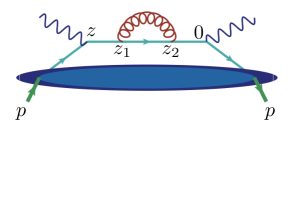
Figure 3: Self-energy correction to the quark propagator

It should be noted that the quark self-energy diagram (see Fig.  3) cannot be factorized into a tree-level coefficient function and the matrix element $\langle p|\bar{\psi}(0)\ldots A^{\alpha_{1}}(z_{1})\ldots A^{\alpha_{1}}(z_{2})\ldots\psi(z)|p\rangle$. Its entire contribution belongs to the one-loop part of the coefficient function. This means that the definition (2.17) of ${M}^{\alpha}(z,p)$ should imply that the $A^{\alpha_{i}}(t_{i}z)$-fields in the expansion of the exponential (2.14) are not contracted with each other. In other words, the contributions corresponding to the link self-energy corrections (see Fig. 4) should be excluded.

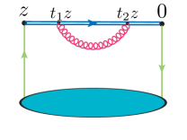
Figure 4: Self-energy correction to the gauge link.

However, when the matrix element (2.17) is calculated on the lattice, such contributions are included automatically: the lattice “does not know” about this restriction. Moreover, the link self-energy diagram produces ultraviolet divergences when $z$ is off the light cone. These divergences require an additional UV regularization. Fortunately, these divergences (and also link-vertex UV divergences) are multiplicative[38, 39, 40, 41, 42, 43, 44] (see also recent papers [45, 46, 47]). They form a factor $Z(-z^{2}/a^{2})$, where $a$ is a UV cut-off, e.g., the lattice spacing. This factor should be included in the right-hand side of the OPE (2.10). Thus, to get the PDF $f(x,\mu^{2})$ from the pseudo-PDF ${\cal P}(x,-z^{2})$ one should “renormalize” the latter by dividing it by $Z(-z^{2}/a^{2})$.

2.4 Ioffe-time distributions

The pseudo-PDF representation (2.2) separates the dependence $M(z,p)$ on its two $z$-dependent Lorentz invariants, the Ioffe time $(pz)\equiv-\nu$ and the interval $z^{2}$ (see Fig. 5). Writing $M(z,p)$ as a function of $\nu$ and $z^{2}$, we get the Ioffe-time pseudodistribution ${\cal M}(\nu,-z^{2})$. Inverting Eq. (2.2) gives the relation

$${\cal P}(x,-z^{2}) =\frac{1}{2\pi}\,\int_{-\infty}^{\infty}\differential\nu\,e^{-ix\nu}\,{\cal M}(\nu,-z^{2})$$ (2.20)

that tells us that the pseudo-PDF is a Fourier transform of the pseudo-ITD ${\cal M}(\nu,-z^{2})$ with respect to $\nu$ for fixed $z^{2}$. When $z$ is on the light cone, $z^{2}=0$, we deal with the light-cone PDF $f(x,\mu^{2})$ and the light-cone Ioffe-time distribution

$${\cal I}(\nu,\mu^{2})=\int_{-1}^{1}\differential x\,e^{ix\nu}\,f(x,\mu^{2})\,$$ (2.21)

introduced originally in Ref. [12]. In terms of the ITDs, the factorization relation (2.10) takes the form

$${\cal M}(\nu,-z^{2})/Z(-z^{2}/a^{2})= \int_{-1}^{1}{\differential w}\,C(w,z^{2}\mu^{2})\,{\cal I}(w\nu,\mu^{2})+{\cal O}(z^{2})\ .$$ (2.22)

Combining (2.22) and (2.21), we obtain a kernel relation

$${\cal M}(\nu,-z^{2})/Z(-z^{2}/a^{2})= \int_{-1}^{1}{\differential x}\,R(x\nu,-z^{2}\mu^{2})\,{f}(x,\mu^{2})+{\cal O}(z^{2})\$$ (2.23)

that directly connects the renormalized pseudo-ITD with the light-cone PDF through the kernel

$$R(x\nu,-z^{2}\mu^{2})= \int_{-1}^{1}{\differential w}\,e^{iwx\nu}\,C(w,z^{2}\mu^{2})\,\ .$$ (2.24)

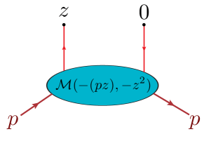
Figure 5: Ioffe-time distribution.

The pseudo-PDF strategy is to start with the standard lattice choice[2, 3, 4] of taking an equal-time interval $z=\{0,0,0,z_{3}\}$ and extract the ${\cal M}(\nu,-z^{2})$ as a function of $\nu$ and $z^{2}$. As we discussed, it is the $\nu$-dependence of ${\cal M}(\nu,-z^{2})$ that governs the $x$-dependence of PDFs. When $z=\{0,0,0,z_{3}\}$, we have $\nu=p_{3}z_{3}$ and $z^{2}=-z_{3}^{2}$.

The basic idea of the pseudo-PDF approach is that it does not matter if $\nu$ is given by $-p_{+}z_{-}$ or by $p_{3}z_{3}$. In both cases, one deals with the same functional dependence of ${\cal M}(\nu,-z^{2})$ on $\nu$. Using the relations (2.22), (2.23), we can (at least, in principle) extract light-cone functions $f(x,\mu^{2})$ from the “Euclidean” pseudo-PDF ${\cal M}(\nu,z_{3}^{2})$.

It is worth stressing here that the applicability of the basic perturbative relations (2.22), (2.23) is determined solely by the size of $z_{3}^{2}$. One can take small $p_{3}$ (even $p_{3}=0$), and use perturbative QCD as far as $z_{3}^{2}$ is sufficiently small. The size of the momentum $p_{3}$ changes the magnitude of $\nu=p_{3}z_{3}$, but it does not affect the applicability of the perturbative expansion.

Another key element of the pseudo-PDF approach is the elimination of the problematic UV $Z$-factor by introducing[11] the reduced Ioffe-time pseudodistribution

$${\mathfrak{M}}(\nu,z_{3}^{2})\equiv\frac{{\cal M}(\nu,z_{3}^{2})}{{\cal M}(0,z_{3}^{2})}\ .$$ (2.25)

Since $Z(z_{3}^{2}/a^{2})$ does not depend on $\nu$, the $Z$-factors of the numerator and denominator cancel. The remaining $z_{3}^{2}$-dependence of ${\mathfrak{M}}(\nu,z_{3}^{2})$ for small $z_{3}^{2}$ is completely determined by the evolution logarithms, and may be calculated perturbatively using OPE in the form of Eqs. (2.22), (2.23). Note also that the denominator factor

$${\cal M}(0,z_{3}^{2})=\int_{-1}^{1}\differential x\,{\cal P}(x,z_{3}^{2})\,$$ (2.26)

is just the lowest moment of the pseudo-PDF. Thus, there is nothing singular here in taking $p_{3}=0$. Moreover, if the local limit $z_{3}\to 0$ corresponds to a conserved current, then ${\cal M}(0,z_{3}^{2})$ does not have the evolution $z_{3}^{2}$-dependence, which provides a further simplification.

The ratio (2.25) may be also used for elimination of the $Z(z_{3}^{2}/a^{2})$-factor in the quasi-PDF approach discussed in the next Section. However, the quasi-PDF practitioners prefer to use the RI/MOM method (see Ref. [16] for a review), in which ${\cal M}(\nu,z_{3}^{2})$ is divided by the matrix element $m(z_{3},p_{R})=\langle p_{R}|{\cal O}(z_{3})|p_{R}\rangle$ of the same bilocal operator ${\cal O}(z_{3})$ sandwiched between parton (quark or gluon) states taken at some reference momentum $p_{R}$. A usual choice is to take spacelike $p_{R}$ with large virtuality, which raises the questions about gauge invariance of such matrix elements. This difficulty is avoided if ${\cal M}(\nu,z_{3}^{2})$ is divided by the vacuum matrix element $\langle 0|{\cal O}(z_{3})|0\rangle$, as suggested in Ref. [48]. Still, both of these alternatives have the disadvantage that the denominator of the ratio should be obtained from a separate calculation, and this increases systematic errors.

2.5 Quasi-PDFs

To define the parton quasi-distribution functions[4] or quasi-PDFs $Q(y,P)$, one takes the separation $z=\{0,0,0,z_{3}\}$ and momentum $p=(E,{\bf 0}_{\perp},P)$ in the same direction. Then $Q(y,P)$ is given by the Fourier transform of the matrix element $M(z_{3},P)$ with respect to $z_{3}$

$$Q(y,P) =\frac{P}{2\pi}\,\int_{-\infty}^{\infty}dz_{3}\,e^{-iyPz_{3}}\,M(z_{3},P)\ .$$ (2.27)

The inverse representation has the form of a plane-wave decomposition

$$M(z_{3},P)= \int_{-\infty}^{\infty}dy\,e^{iyPz_{3}}\,Q(y,P)\,$$ (2.28)

in which the function $Q(y,P)$ describes what fraction $yP$ of the hadron’s third momentum component is carried by a specified parton.

It is easy to find a relation between the quasi-PDF $Q(y,P)$ and the pseudo-PDF ${\cal P}(x,z_{3}^{2})$ corresponding to the $z=z_{3}$ separation. Indeed, adjusting the definition (2.2) of the pseudo-PDF to this particular case,

$$M(z_{3},p) =\int_{-1}^{1}dx\,e^{ixz_{3}P}\,{\cal P}(x,z_{3}^{2})\ ,$$ (2.29)

and using this result in the definition (2.27) of the quasi-PDF gives

$$Q(y,P)=\frac{P}{2\pi}\int_{-1}^{1}dx\,\int_{-\infty}^{\infty}dz_{3}\,e^{-i(y-x)Pz_{3}}\,{\cal P}(x,z_{3}^{2})\ .$$ (2.30)

This expression shows that the quasi-PDFs $Q(y,P)$ are defined on the whole real $y$-axis, despite the fact that the pseudo-PDFs ${\cal P}(x,z_{3}^{2})$ have support on the limited segment $-1\leq x\leq 1$ only.

Another straightforward, but important observation is that when a pseudo-PDF does not depend on its second variable, $z_{3}^{2}$, i.e., if ${\cal P}(x,z_{3}^{2})=f(x)$, then the integral over $z_{3}$ in Eq. (2.30) gives $\delta(y-x)/P$, so that the resulting quasi-PDF $Q(y,P)$ has no dependence on $P$ and coincides with the light-cone distribution $f(y)$.

Alternatively, when ${\cal P}(x,z_{3}^{2})$ depends on $z_{3}^{2}$, the integral over $z_{3}$ gives a nontrivial function

$$R(x,y-x,P)\equiv\frac{P}{2\pi}\int_{-\infty}^{\infty}dz_{3}\,e^{-i(y-x)Pz_{3}}\,{\cal P}(x,z_{3}^{2})\$$ (2.31)

that produces $Q(y,P)$ after the subsequent $x$-integration,

$$Q(y,P)=\int_{-1}^{1}dx\,R(x,y-x,P)\ .$$ (2.32)

Thus, it is the $z_{3}^{2}$-dependence of ${\cal P}(x,z_{3}^{2})$ (or, equivalently, of ${\cal M}(\nu,z_{3}^{2})$) that is responsible for the deviation of quasi-PDFs from lightcone PDFs. In particular, it generates the parts of $Q(y,P)$ outside the PDF support region $|y|\leq 1$.

Eq. (2.32) has a simple physical interpretation: the fraction $yP$ of the third momentum component carried by the parton comes from two sources: (i) from the longitudinal motion of the hadron as a whole (which gives $xP$), and (ii) from the part $(y-x)P$ that is generated by a nontrivial dependence of ${\cal P}(x,z_{3}^{2})$ on $z_{3}^{2}$. In its turn, the $z^{2}$-dependence of ${\cal P}(x,-z^{2})$ is related to spatial distribution of partons inside hadrons.

2.6 Transverse Momentum Dependent PDFs

Recall that ${\cal P}(x,-z^{2})$ is a function defined in a covariant manner by Eq. (2.2). This means that if we choose the spacelike part of $z$ in a plane $z_{\perp}=\{z_{1},z_{2}\}$ perpendicular to the $z_{3}$ direction, the resulting pseudo-PDF will be given by ${\cal P}(x,z_{\perp}^{2})$, i.e., by the same function, but with $z_{3}^{2}$ substituted by $z_{\perp}^{2}$. As a result, it is possible to show that the pseudo-PDF ${\cal P}(x,-z^{2})$ for space-like $z$ has a simple interpretation in terms of the transverse momentum-dependent (TMD) PDFs.

Take again the frame where $p=(E,{\bf 0}_{\perp},P)$ and choose a separation $z$ for which the lightcone component $z_{+}$ vanishes, $z_{+}=0$, and only $z_{-}$ and $z_{\perp}=\{z_{1},z_{2}\}$ are non-zero. With this choice, we have $\nu=-p_{+}z_{-}$ for the Ioffe time, and $z^{2}=-z_{\perp}^{2}$ for the interval. The TMD can be defined in a standard way through a two-dimensional Fourier transform with respect to $z_{\perp}$, which gives

$${\cal P}(x,z_{\perp}^{2}) =\int{d^{2}k_{\perp}}\,e^{-i(k_{\perp}z_{\perp})}{\cal F}(x,k_{\perp}^{2})\$$ (2.33)

when inverted. This is equivalent to the following representation of the original matrix element,

$${\cal M}(\nu,z_{\perp}^{2}) =\int_{-1}^{1}dx\,\,e^{ix\nu}\int{d^{2}k_{\perp}}\,e^{-i(k_{\perp}z_{\perp})}{\cal F}(x,k_{\perp}^{2})\ .$$ (2.34)

Due to the invariance with respect to rotations in the $z_{\perp}$ plane, the TMD defined in this way depends on $k_{\perp}^{2}$ only.

Eq. (2.34) corresponds to a plane-wave decomposition in which the parton carries a longitudinal $xp_{+}$ fraction (with $-1\leq x\leq 1$), but it also has a transverse momentum $k_{\perp}$. Since $k_{\perp}$ is Fourier-conjugate to $z_{\perp}$, we may say that the transverse momentum dependence of TMDs is governed by the $z^{2}$-dependence of pseudo-ITDs. Similarly, the dependence of ${\cal M}(\nu,z_{\perp}^{2})$ on $\nu$ governs the $x$-dependence of ${\cal F}(x,k_{\perp}^{2})$, i.e. the longitudinal momentum structure of the hadron.

Though the definition of the quasi-PDF is based on a matrix element involving a purely “longitudinal” separation $z=z_{3}$, the Lorentz invariance tells us that the dependence of ${\cal M}(\nu,z_{3}^{2})$ on $z_{3}^{2}$ is given by the same function that defines the TMD by Eq. (2.34). This observation allows us to get a relation between quasi-PDFs and TMDs. To this end, we take $z_{\perp}=\{0,\nu/P\}$ in Eq. (2.34) and insert the resulting representation into the definition (2.27) of the quasi-PDF. We obtain [14, 11]

$$Q(y,P)= \,P\int_{-1}^{1}dx\,\int_{-\infty}^{\infty}dk_{1}{\cal F}(x,k_{1}^{2}+(y-x)^{2}P^{2})\ .$$ (2.35)

This relation shows again that the quasi-PDF variable $y$ has the $-\infty<y<\infty$ support, simply because the value of the transverse momentum component $k_{2}$ in ${\cal F}(x,k_{1}^{2}+k_{2}^{2})$ is not limited.

We also see once more that the third component $k_{3}=yP$ of the parton momentum is composed from the part $xP$, coming from the motion of the hadron as a whole, and the remaining fraction $(y-x)P$ coming from the same physics that generates the transverse momentum dependence of the TMDs.

2.7 TMD parametrization

Since the pseudo-PDF ${\cal P}(x,z_{\perp}^{2})$ defining the TMD ${\cal F}(x,k_{\perp}^{2})$ has the same functional form as the pseudo-PDF ${\cal P}(x,-z^{2})$ for a general spacelike $z$, we can use TMDs to parametrize the $z^{2}$-dependence of a generic matrix element $M(z,p)$ for an arbitrary spacelike $z$. To this end, let us take the TMD definition (2.33) and integrate over the angle between ${\bf k}_{\perp}$ and ${\bf z}_{\perp}$. This gives

$${\cal P}(x,z_{\perp}^{2}) =2\pi\,\int_{0}^{\infty}\,dk_{\perp}\,k_{\perp}J_{0}\left(k_{\perp}z_{\perp}\right)\,{\cal F}(x,k_{\perp}^{2})\ ,$$ (2.36)

where $J_{0}$ is the Bessel function. Use now the fact that ${\cal P}(x,-z^{2})$ is a function defined by a covariant relation (2.2). This implies that, for a general spacelike $z$, one can write the representation for the generic matrix element $M(z,p)$ in terms of the TMD,

$$\langle p| \phi(0)\phi(z)|p\rangle=\,2\pi\,\int_{-1}^{1}dx\,e^{-ix(pz)}\int_{0}^{\infty}\,dk\,k\,J_{0}\left(k\sqrt{-z^{2}}\right)\,{\cal F}(x,k^{2})\ .$$ (2.37)

Here, we intentionally dropped “$\perp$” in the notation for the momentum variable. By this change, we stress that $k$ is just an integration parameter of this representation. While ${\cal F}(x,k^{2})$ is a function that coincides with the TMD, one does not need to specify a “transverse” plane and treat $k$ as the magnitude of a 2-dimensional momentum in that plane.  In particular, nothing prevents us from choosing $z$ in a purely longitudinal direction, i.e. from taking $z=\{0,0,0,z_{3}\}$. Then we can write

$$\langle p| \phi(0)\phi(z_{3})|p\rangle=\,2\pi\,\int_{-1}^{1}dx\,e^{ixPz_{3}}\int_{0}^{\infty}dk\,k\,J_{0}\left(kz_{3}\right)\,{\cal F}(x,k^{2})\$$ (2.38)

without asking (or answering) the question: in which plane “$k$” is supposed to be? As written, “$k$” is just a scalar variable in a particular representation (2.38) for the matrix element.

2.8 Taylor expansion

The TMD parametrization (2.37) is very general. It just reflects the Lorentz invariance (the fact that matrix element $M(z,p)$ depends on $(pz)$ and $z^{2}$) and spectral properties of Feynman diagrams (the limits on $x$ are $-1\leq x\leq 1$), as given by the underlying pseudo-PDF representation (2.2). It holds for any diagram, whether it is regular for $z^{2}=0$, or has $\ln(-z^{2})$ singularities.

However, it is instructive to give a derivation of Eq. (2.2) for the case when the matrix elements $M(z,p)$ is regular for $z=0$ to the extent that all the coefficients of a formal Taylor expansion

$$\langle p|\phi(0)\phi(z)|p\rangle=\sum_{N=0}^{\infty}\frac{1}{N!}z_{\mu_{1}}\ldots z_{\mu_{N}}\ \langle p|\phi(0)\,{\partial}^{\mu_{1}}\ldots{\partial}^{\mu_{N}}\phi(0)|p\rangle\$$ (2.39)

are finite. Now the information about the hadron is contained in the matrix elements
$\langle p|\phi(0){\partial}^{\mu_{1}}\ldots{\partial}^{\mu_{N}}\phi(0)|p\rangle$ of local operators. Due to Lorentz invariance, they may be written as

$$\langle p|\phi(0){\partial}^{\mu_{1}}\ldots {\partial}^{\mu_{N}}\phi(0)|p\rangle=(-i)^{N}\,p^{\mu_{1}}\ldots p^{\mu_{n}}\,A_{N}^{(0)}$$

$$+{\rm terms\ containing}\ g^{\mu_{i}\mu_{j}}\ .$$ (2.40)

Utilizing the fact that the $\mu_{k}$ indices are symmetrized in the Taylor expansion by the $z_{\mu_{1}}\ldots z_{\mu_{n}}$ factor, we may use a more organized expression

$$\langle p|\phi(0)(z\partial)^{N}\phi(0)|p\rangle=(-i)^{N}\sum_{l=0}^{[N/2]}(-z^{2}\Lambda^{2})^{l}(pz)^{N-2l}A_{N}^{(l)}\ .$$ (2.41)

The information about the hadron structure is now accumulated in the constants $A_{N}^{(l)}$. The momentum scale $\Lambda$ is introduced to secure that all $A_{N}^{(l)}$’s have the same dimension. In general, one needs $[N/2]$ (the integer part of $N/2$) constants to parametrize this matrix element. Treating the constants $A_{N}^{(l)}$ as $x^{N}$ moments of some functions $F_{l}(x)$

$$A_{N}^{(l)}=\frac{N!}{(N-2l)!}\int_{-1}^{1}dx\,x^{N-2l}\,F_{l}(x)\ ,$$ (2.42)

we obtain the desired pseudo-PDF representation for the matrix element,

$$\langle p|\phi(0)\phi(z)|p\rangle= \int_{-1}^{1}dxe^{-ix(pz)}\,\sum_{l=0}^{\infty}(-z^{2}\Lambda^{2})^{l}F_{l}(x)$$

$$\equiv\int_{-1}^{1}dxe^{-ix(pz)}\ {\cal P}(x,-z^{2})\ .$$ (2.43)

As we have seen in Section 2.1, the lowest $l=0$ term produces the twist-2 contribution to the forward Compton amplitude The function $F_{0}(x)\equiv f(x)$ coincides with the twist-2 light-cone PDF.

2.9 Twist decomposition

Usually the twist-2 contribution (2.6) for DIS is obtained using the twist decomposition, which is a standard way to parametrize the $z^{2}$-dependence of the generic matrix element. It involves expansion of $z^{\mu_{1}}\ldots z^{\mu_{n}}$ factor in Eq. (2.39) over traceless tensors $\{z_{\mu_{1}}\ldots z_{\mu_{n}}\}$. In the case of scalar fields, it is possible to derive [49]

$$\langle p|\phi(0)\phi(z)|p\rangle= \sum_{l=0}^{\infty}\left(\frac{z^{2}}{4}\right)^{l}\sum_{N=0}^{\infty}\frac{N+1}{l!(N+l+1)!}\langle p|\phi(0)\{z{\partial}\}^{N}({\partial}^{2})^{l}\phi(0)|p\rangle\ ,$$ (2.44)

where we use the notation

$$\{z\partial\}^{n}\equiv\{z_{\mu_{1}}\ldots z_{\mu_{n}}\}\,\partial^{\mu_{1}}\ldots\partial^{\mu_{n}}\ .$$ (2.45)

We can parametrize the matrix elements entering Eq. (2.44) by

$$\langle p|\phi(0)\{z{\partial}\}^{N}({\partial}^{2})^{l}\phi(0)|p\rangle=\lambda^{2l}(-i)^{N}\{zp\}^{N}\,B_{N}^{(l)}\ ,$$ (2.46)

where the overall scale $\lambda$ with the dimension of mass is introduced in order to have the coefficients $B_{N}^{(l)}$ with the same dimension. This gives the twist decomposition

$$\langle p|\phi(0)\phi(z)|p\rangle= \sum_{l=0}^{\infty}\frac{1}{l!}\,\left(\frac{\lambda^{2}z^{2}}{4}\right)^{l}\sum_{N=0}^{\infty}\frac{N+1}{(N+l+1)!}\,(-i)^{N}\{zp\}^{N}\,B_{N}^{(l)}\$$ (2.47)

involving the powers of $z^{2}$ and traceless combinations $\{zp\}^{N}$.

Alternatively, if one applies the Taylor expansion to $e^{-ix(pz)}$ and the Bessel function $J_{0}\left(k\sqrt{-z^{2}}\right)$ of the TMD representation (2.37), one gets a series which also involves the powers of $z^{2}$, but they are accompanied by simple powers $(zp)^{N}$,

$$\langle p| \phi(0)\phi(z)|p\rangle=\sum_{l=0}^{\infty}\frac{1}{(l!)^{2}}\left(\frac{\Lambda^{2}z^{2}}{4}\right)^{l}\,\sum_{N=0}^{\infty}\frac{1}{N!}\,(-i)^{N}(zp)^{N}\,C_{N}^{(l)}\ .$$ (2.48)

The coefficients $C_{N}^{(l)}$ here are the combined moments of the TMD

$$C_{N}^{(l)}=\,2\pi\,\int_{-1}^{1}dx\,x^{N}\int_{0}^{\infty}\,dk\,k\,(k^{2})^{l}\,{\cal F}(x,k^{2})\ .$$ (2.49)

To shorten formulas, we may switch here back $k\to k_{\perp}$ in the notation for the integration variable, and also write the resulting $2\pi k_{\perp}dk_{\perp}$ as $d^{2}k_{\perp}$. We can do this because the TMD ${\cal F}(x,k_{\perp}^{2})$ does not depend on the polar angle. Then

$$C_{N}^{(l)}=\int_{-1}^{1}dx\,x^{N}\int_{0}^{\infty}\,d^{2}k_{\perp}\,(k_{\perp}^{2})^{l}\,{\cal F}(x,k_{\perp}^{2})\equiv\langle x^{N}k_{\perp}^{2l}\rangle_{\cal F}\ .$$ (2.50)

We emphasize again that $k$ or $k_{\perp}$ should be understood simply as scalar integration variables. We do not need to specify in which plane $k_{\perp}$ is.

An obvious advantage of the TMD representation (2.37) is that, unlike the twist decomposition (2.47), it displays the $z$-dependence of $M(z,p)$ by a closed formula rather than by a double series. Furthermore, the $(pz)$-dependence in Eq. (2.37) comes through the plane waves $e^{-ix(pz)}$. As a result, most integrals over $z$ (such as the integral (2.27) producing quasi-PDFs) are straightforward.

In contrast, the twist decomposition (2.47) is a series expansion over combinations $\{pz\}^{n}$ involving a rather complicated traceless tensor $\{z_{\mu_{1}}\ldots z_{\mu_{n}}\}\$. This results in an involved procedure for integrations over $z$. Furthermore, the task of summing series in $\{pz\}^{n}$ structures into a closed form is rather tricky. In fact, even when successful, the results of such a summation involve imaginary exponentials of $(pz)\pm\sqrt{(pz)^{2}-p^{2}z^{2}}$ which are next to impossible to integrate in a general case.

Another practical advantage of the TMD representation is that it describes the $z^{2}$-dependence through Eq. (2.37) involving a “spectral function” ${\cal F}(x,k^{2})$ that has a clear physical interpretation of a transverse momentum distribution. Based on this interpretation, one may expect that ${\cal F}(x,k^{2})$ is a function finite for $k=0$ and monotonically decreasing with $k$ when $k$ increases. One should not expect oscillations or other exotics in its $k$-dependence.

Taking some model for ${\cal F}(x,k^{2})$, one can get a model for the pseudo-PDF,

$${\cal P}(x,-z^{2})=\,2\pi\,\int_{0}^{\infty}\,dk\,k\,J_{0}\left(k\sqrt{-z^{2}}\right)\,{\cal F}(x,k^{2})\ .$$ (2.51)

The pseudo-PDF representation (2.2) gives then a model for the ITD.

3 Nonperturbative evolution of soft quasi-PDFs

Having a model for ${\cal F}(x,k^{2})$ and using the quasi-PDF/TMD relation (2.35), one can get a model for the quasi-PDF and study qualitative features of possible $P$-dependence patterns of the quasi-PDFs $Q(y,P)$. Such models were proposed originally in our paper [14].

3.1 Models for soft quasi-PDFs

Since our goal is to study general features of the $P$-dependence, it makes sense to take simple, but still realistic models. In this respect, the collinear model ${\cal F}(x,k_{\perp}^{2})=f(x)\delta(k_{\perp}^{2})/\pi$ is not realistic, since it gives $\langle k_{\perp}^{2}\rangle=0$. Next in complexity are factorized models, in which ${\cal F}(x,k_{\perp}^{2})$ is given by a product

$${\cal F}(x,k_{\perp}^{2})=f(x)K(k_{\perp}^{2})$$ (3.1)

of a collinear PDF $f(x)$ and a $k_{\perp}^{2}$-dependent factor $K(k_{\perp}^{2})$. Such models are used on a daily basis by TMD practitioners (see, e.g. Ref. [50]), with the Gaussian form

$$K_{G}(k_{\perp}^{2})= \frac{1}{\pi\Lambda^{2}}e^{-k_{\perp}^{2}/\Lambda^{2}}$$ (3.2)

being the most popular choice. For the Ioffe-time pseudo-distribution ${\cal M}(\nu,z_{3}^{2})$, this corresponds to the factorized Ansatz

$${\cal M}^{\rm soft}(\nu,z_{3}^{2})={\cal I}^{\rm soft}(\nu,0){\cal M}(0,z_{3}^{2})\$$ (3.3)

for its soft part. In this case, the soft part of the reduced ITD ${\mathfrak{M}}(\nu,z_{3}^{2})$ does not have $z_{3}^{2}$-dependence and coincides with ${\cal I}^{\rm soft}(\nu,0)$. While there seem to be no first-principle reasons for such a factorization property for ${\cal M}^{\rm soft}(\nu,z_{3}^{2})$, it has been actually observed in a recent lattice study of the Ioffe-time pseudo-distributions in Ref. [17]. It is also supported by the pioneering study[51] of the TMDs in the lattice QCD performed a decade ago.

Using the factorized model (3.1) with the Gaussian shape (3.2) gives the following model for the quasi-PDF

$$Q_{G}(y,P)= \frac{P}{\Lambda\sqrt{\pi}}\,\int_{-1}^{1}dx\,f(x)\,e^{-(x-y)^{2}P^{2}/\Lambda^{2}}\ .$$ (3.4)

It is instructive to choose $f(x)$ in the form

$$f(x)=\frac{315}{32}\,\sqrt{x}(1-x)^{3}\theta(x>0)$$ (3.5)

obtained in Ref. [17] for the soft part of the $u_{v}(x)-d_{v}(x)$ nucleon PDF. It was extracted from the lattice data using the pseudo-PDF-based method proposed in our paper [11]. Our goal is to investigate, what kind of quasi-PDFs one would get for such a PDF in the Gaussian factorized model.

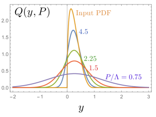
Figure 6: Evolution of $Q(y,P)$ in the Gaussian model for $P/\Lambda=0.75,1.5,2.25,4.5$ compared to the limiting PDF $f(y)=\frac{315}{32}\,\sqrt{y}(1-y)^{3}$.

The curves are shown in Fig. 6. One can see that the quasi-PDFs have large parts outside the support segment $0\leq y\leq 1$ of the input PDFs. As we have already emphasized in Sec. IIF, it is the $z_{3}^{2}$ dependence of the pseudo-ITD ${\cal M}(\nu,z_{3}^{2})$ that generates those parts of the quasi-PDFs that are outside the $-1\leq y\leq 1$ region. When $P$ increases, the quasi-PDFs in Fig. 6 shrink inside the $0\leq y\leq 1$ segment. In particular, the area under the negative-$y$ part of $Q^{\rm soft}(y,P)$ quickly decreases for large $P$, and vanishes in the $P\to\infty$ limit.

The change of quasi-PDFs with $P$ in our Gaussian model is very close to that actually observed in the lattice QCD calculations for the $u_{v}(x)-d_{v}(x)$ nucleon PDF reported in Ref. [52]. In fact, our curves corresponding to $P/\Lambda$ in multiples of 0.75, namely for $P/\Lambda=0.75,1.5,2.25$ are close to the curves of Ref. [52] obtained for the momentum values in the same 1, 2, 3 multiples of $p=2\pi/L$ (i.e., for $p=2\pi/L,4\pi/L,6\pi/L$, correspondingly). This is a very suggestive indication that the major role in forming the observed shape of quasi-PDFs is played by the non-perturbative physics reflecting the hadron size.

Looking at the curves shown in Fig. 6, one sees that the maximal value of the quasi-PDF $Q(y,P)$ for $P=2.25\Lambda$ is more than twice lower than the maximal value of the input PDF. A natural conclusion is that the $P=2.25\Lambda$ momentum is simply too small. Namely, to convert $Q(y,P=2.25\Lambda)$ into the input PDF, one needs corrections of the same size as the $Q(y,P=2.25\Lambda)$ quasi-PDF itself. It is necessary to at least double $P$ to get a quasi-PDF that is sufficiently close to the limiting PDF form. Only then one may have some hope that the remaining gap may be fixed by adding corrections that are not too large compared to the starting approximation.

Larger values of $P$, namely, $P=10\pi/L$, were reached in the lattice calculation of Ref. [53]. One may check that the quasi-PDF obtained in that paper is very close to the $P/\Lambda=4.5$ curve of Fig. 6. While being much closer to the input PDF, the $P/\Lambda=4.5$ curve still shows strong artifacts of unfinished nonperturbative evolution, in particular, a rather large signal for negative $y$.

From the value $P=1.29$ GeV indicated in Ref. [52] for the highest momentum $p=6\pi/L$, we can also estimate the magnitude $\Lambda^{2}\approx(600$ MeV)² of the effective Gaussian parameter. This is much larger than $\langle k_{\perp}^{2}\rangle\approx(300$ MeV)² that one would expect from the transverse momentum distribution. However, ${\cal M}^{\rm soft}(\nu,z_{3}^{2})$ in this case reflects both the $z_{3}$-dependence induced by the nonperturbative dependence of TMDs and also the $z_{3}$ dependence of the gauge-link-related $Z(z_{3}^{2}/a^{2})$ factor. The latter was not removed in the calculation of Ref. [52].

A more recent lattice calculation [54] includes renormalization of the link-related UV singularities. This procedure should eliminate, to some extent, the nonperturbative $z_{3}^{2}$-dependence of the $Z(z_{3}^{2}/a^{2})$ factor from the renormalized data. Still, the $z_{3}^{2}$-dependence induced by the transverse-momentum distribution may be there. Indeed, the quasi-PDF shown in Fig. 29 of Ref. [54] has all the features of unfinished nonperturbative evolution.

3.2 Rate of approach

One may also be interested in which way the finite-$P$ quasi-PDF curves approach the limiting PDF curve. To get the answer in a short analytic form, let us take a very simple input PDF $f(x)=1-x$ and the same Gaussian Ansatz (3.2) for the $k_{\perp}$-dependence. In this case, we have

$$Q(y,P)= \frac{1}{2}(1-y)\Big{[}\text{erf}\left[{(1-y)}P/{\Lambda}\right]+\text{erf}\left[{y}P/{\Lambda}\right]\Big{]}$$

$$+\frac{\Lambda}{2\sqrt{\pi}P}\left[e^{-{(1-y)^{2}}P^{2}/{\Lambda^{2}}}-e^{-{y^{2}}P^{2}/{\Lambda^{2}}}\right]\ ,$$ (3.6)

where the error function is defined by

$$\text{ erf}(z)=\frac{2}{\sqrt{\pi}}\int_{0}^{z}dt\,e^{-t^{2}}\ .$$ (3.7)

For large $z$, it may be approximated by

$$\text{ erf}(z)=1-\frac{e^{-z^{2}}}{\sqrt{\pi}z}\left[1-\frac{1}{2z^{2}}-\ldots\right]\ .$$ (3.8)

As a result, the approach to the $P\to\infty$ limit is governed by the exponentials $e^{-(1-y)P^{2}/\Lambda^{2}}$ and $e^{-yP^{2}/\Lambda^{2}}$. In particular, at the middle of the $0\leq y\leq 1$ interval, we have

$$Q(1/2,P)=\frac{1}{2}\text{erf}\left(\frac{P}{2\Lambda}\right)=\frac{1}{2}-\frac{\Lambda e^{-P^{2}/4\Lambda^{2}}}{\sqrt{\pi}P}\left[1-\frac{2\Lambda^{2}}{P^{2}}-\ldots\right]\ .$$ (3.9)

Thus, the approach to the limiting value is exponential $\sim e^{-P^{2}/4\Lambda^{2}}$ rather than a powerlike.

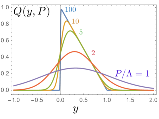
Figure 7: Evolution of $Q(y,P)$ in the Gaussian model for $P/\Lambda=1,2,5,10,100$. The limiting PDF is $f(y)=(1-y)$.

At the end-points, one of the exponentials converts into 1, so these are special cases. The input PDF $f(y)=1-y$ vanishes for $y=1$, and the quasi-PDF approaches this limit according to

$$Q(1,P)= \frac{\Lambda}{2\sqrt{\pi}P}\left[1-e^{-{P^{2}}/{\Lambda^{2}}}\right]\ ,$$ (3.10)

i.e. like $\sqrt{\Lambda^{2}/P^{2}}$ rather than $\Lambda^{2}/P^{2}$. The non-analytic behavior with respect to $\Lambda^{2}/P^{2}$ is present at another end-point as well

$$Q(0,P)=\frac{1}{2}\text{erf}\left(\frac{P}{\Lambda}\right)+\frac{\Lambda}{2\sqrt{\pi}P}\left[1-e^{-{P^{2}}/{\Lambda^{2}}}\right]$$

$$=\frac{1}{2}+\frac{\Lambda}{2\sqrt{\pi}P}\left[1-2e^{-{P^{2}}/{\Lambda^{2}}}\left(1-\frac{\Lambda^{2}}{4P^{2}}-\ldots\right)\right]\ .$$ (3.11)

As one can see, at $y=0$, the quasi-PDF approaches 1/2, the average of its $0_{+}$ and $0_{-}$ limits of the input PDF at that point. The curves for $Q(y,P)$ in this model are shown in Fig. 7.

It is also instructive to look at the curves illustrating the $P$-dependence of quasi-PDFs at particular values of $y$ (see Fig. 8). It is clear that having just three points, at $P/\Lambda=0.75,1.5$ and 2.25, it is rather difficult to make an accurate extrapolation to correct $P=\infty$ values.

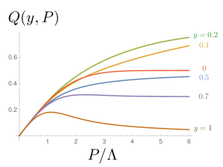
Figure 8: $P$-dependence of $Q(y,P)$ in the Gaussian model for indicated values of $y$.

Summarizing, we see that the $k_{\perp}$ effects generate a very nontrivial pattern of nonperturbative evolution of the quasi-PDFs $Q(y,P)$. We also observed that, in the case of a Gaussian TMD, this evolution cannot be described by a ${\cal O}(\Lambda^{2}/P^{2})$ corrections on the point-by-point basis in $y$-variable.

3.3 Expansion in $1/P^{2l}$

Using the TMD parametrization (2.38), we can write a formal $1/P^{2l}$ expansion for the quasi-PDF $Q(y,P)$

$$Q(y,P)\Rightarrow f(y)+\sum_{l=1}^{\infty}\int d^{2}k_{\perp}\frac{k_{\perp}^{2l}}{4^{l}P^{2l}(l!)^{2}}\,\frac{\partial^{2l}}{\partial y^{2l}}{\cal F}(y,k_{\perp}^{2})\ .$$ (3.12)

Thus, the scale $\Lambda^{2}$ characterizing the size of the higher-twist $1/P^{2l}$ corrections is set by the magnitude of the $k_{\perp}^{2l}$ moments of the soft TMD ${\cal F}^{\rm soft}(y,k_{\perp}^{2})$. We attached the subscript “soft” here, because it is evident that the $k_{\perp}^{2l}$ moments diverge for the hard part that has the $\sim 1/k_{\perp}^{2}$ behavior for large $k_{\perp}$. Furthermore, Eq. (3.12), “as is”, has a mathematical meaning only if the TMD decreases faster than any inverse power of $k_{\perp}^{2}$ for large $k_{\perp}$, say, like a Gaussian $e^{-k_{\perp}^{2}/\Lambda^{2}}$ or an exponential $e^{-k_{\perp}/\Lambda}$. Such distributions may be called as “very soft”.

3.4 Target-mass corrections

According to the TMD parametrization (2.38), the difference between the quasi-PDF $Q(y,P)$ and the PDF $f(y)$ in Eq. (3.12) is described by the $k_{\perp}^{2l}$ moments of TMDs. Thus, the size of all the $(\Lambda^{2}/P^{2})^{l}$ corrections in the relation between $Q(y,P)$ and $f(y)$ is determined by these moments, and the scale $\Lambda^{2}$ is set by the average value $\langle k_{\perp}^{2}\rangle_{\cal F}$ of the transverse momentum.

Still, a usual statement [4, 52, 53] is that there are two types of $(1/P^{2})^{l}$ contributions: target-mass corrections $(M^{2}/P^{2})^{l}$ and higher-twist corrections $(\lambda^{2}/P^{2})^{l}$. There is no contradiction. Indeed, while there is no explicit source of target mass corrections visible in the TMD parametrization, such terms do appear if one converts it into the twist decomposition. The latter can be obtained by expanding $(z\partial)^{n}$ in Eq. (2.41) over traceless combinations. Take the simplest nontrivial case $n=2$. Then

$$(z\partial)^{2}= \{z\partial\}^{2}+\frac{1}{4}z^{2}\partial^{2}\ ,$$ (3.13)

where $\{z\partial\}^{2}$ is the notation defined in Eq. (2.45). Parametrizing the matrix element

$$\langle p|\phi(0)\partial^{2}\phi(0)|p\rangle=\lambda^{2}\langle p|\phi(0)\phi(0)|p\rangle.$$ (3.14)

we introduce the higher-twist scale $\lambda^{2}$ generated by $\partial^{2}$. One may interpret $\lambda^{2}$ as the average of $(-k^{2})$, or parton virtuality. By equations of motion, $\partial^{2}\phi=g\psi\phi$, so one may also interpret $\lambda^{2}$ as the average strength of the gluon field $g\psi$. Since powers of $\partial^{2}$ are accompanied by powers of $z^{2}$, one gets $(\lambda^{2}/P^{2})^{l}$ corrections for quasi-PDFs. From this physical interpretation, one would expect that the higher-twist scale $\lambda^{2}$ is close to the average transverse momentum scale $\Lambda^{2}$.

The target mass correction $M^{2}/P^{2}$ appears when one parametrizes the matrix element of the traceless part

$$\langle p|\phi(0)\{z\partial\}^{2}\phi(0)|p\rangle=\{zp\}^{2}\langle x^{2}\rangle_{f}$$ (3.15)

and then expands the traceless combination $\{zp\}^{2}$ over the powers of the usual scalar product $(pz)$ and $z^{2}$,

$$\{zp\}^{2}= (zp)^{2}-\frac{1}{4}z^{2}M^{2}\ .$$ (3.16)

Hence, applying the twist decomposition (3.13) to the matrix element, we have

$$\langle p|\phi(0)(z\partial)^{2}\phi(0)|p\rangle=-\left[(zp)^{2}-\frac{1}{4}z^{2}M^{2}\right]\,\langle x^{2}\rangle_{f}+\frac{z^{2}}{4}\,\lambda^{2}\ .$$ (3.17)

On the other hand, using the TMD parametrization (3.12), we get

$$\langle p|\phi(0)(z\partial)^{2}\phi(0)|p\rangle=-\,(zp)^{2}\,\langle x^{2}\rangle_{f}+\frac{z^{2}}{2}\langle k_{\perp}^{2}\rangle_{\cal F}\ .$$ (3.18)

This gives a relation between the parameters of the TMD parametrization and those of the twist decomposition

$$\,\lambda^{2}+M^{2}\langle x^{2}\rangle_{f}=2\langle k_{\perp}^{2}\rangle_{\cal F}\ .$$ (3.19)

This outcome may be also obtained by a direct application of $\partial^{2}$ to the TMD parametrization (2.37) and then taking $z=0$. In the momentum representation, $\partial^{2}$ results in $(-k^{2})$, the parton virtuality. Thus, we may say that it is given by a kinematical term $(-x^{2}M^{2})$ and a contribution due to the parton’s transverse momentum.

When $\partial^{2}\phi=0$, or for “on-shell” quarks, the average transverse momentum $\langle k_{\perp}^{2}\rangle_{\cal F}$ is completely determined by the proton mass and the twist-2 parton distribution $f(x)$. This was known for a long time[55, 56]. Moreover, it may be shown[57] that, if one neglects all the higher-twist contributions, the TMD can be expressed in terms of the twist-2 PDF $f(x)$

$${\cal F}_{\rm twist-2}(x,k_{\perp}^{2})=-\frac{1}{x\pi M^{2}}\,\ f^{\prime}(x+k_{\perp}^{2}/xM^{2})\ .$$ (3.20)

Since $f(x)$ has the $0\leq x\leq 1$ support, this TMD has a peculiar restriction $k_{\perp}^{2}\leq x(1-x)M^{2}$, conflicting with the expectation that the values of $k_{\perp}$ are not limited.

When the higher twists are nonzero, the question is essentially which basis to choose for $1/P^{2l}$ corrections. If one uses the twist decomposition, then the operators $\phi(\partial^{2})^{l}\phi$ are accompanied by $(\lambda^{2}/P^{2})^{l}$ overall factor, and there are also further target mass corrections in powers of $M^{2}/P^{2}$ generated by traceless structures.

On the other hand, if one chooses the TMD parametrization, then there is only one source of $1/P^{2l}$ corrections. They are produced by the $k_{\perp}^{2l}$ moments of TMDs. In this sense, the TMD ${\cal F}(x,k_{\perp}^{2})$ serves as a generating function for corrections in powers of $\Lambda^{2}/P^{2}$. This is a clear advantage of the TMD parametrization.

Nevertheless, one can imagine a scenario when it would be more preferable to use the twist decomposition. Namely, when the matrix elements of operators with powers of $\partial^{2}$ are much smaller than the target mass correction terms. Then, in particular, the moment $\langle k_{\perp}^{2}\rangle_{\cal F}$ will be dominated by $M^{2}\langle x^{2}\rangle_{f}/2$ and could be calculated from the twist-2 PDF $f(x)$. Thus, it is instructive to make an estimate. Take a simple model for valence quark PDF $f(x)=\frac{35}{32}(1-x)^{3}/\sqrt{x}$, then

$$\frac{M^{2}}{2}\int_{0}^{1}dx\,x^{2}f(x)=\frac{M^{2}}{66}\approx 0.013\,{\rm GeV}^{2}\ .$$ (3.21)

This should be compared to, say, the value ${\langle k_{\perp}^{2}\rangle}_{G}=\Lambda^{2}$, that gives a Gaussian TMD (3.2). Even if one takes $\Lambda$ as small as 300 MeV, $\Lambda^{2}$ is numerically about 0.1  GeV², So, there are no reasons to expect that the target-mass corrections are larger than the $k_{\perp}$ effects. In fact, all the evidence is that they are much smaller.

It should be also emphasized that the “target-mass corrections” appear only within the twist decomposition. The latter may be obtained from the TMD parametrization (2.37) by an artificial procedure of expanding the $e^{-ix(pz)}$ factor there over the traceless combinations $\{pz\}^{k}$. In this sense, the target-mass corrections are created “by hand”. If one chooses to work with the TMD parametrization, there are no kinematical target mass corrections. All the $1/P^{2l}$ corrections are described by the $k_{\perp}^{2l}$ moments of the TMDs.

The same is true for the twist decomposition of the pseudo-PDF representation (2.2): there is no need to expand $e^{-ix(pz)}$ there over $\{pz\}^{k}$.

One may wonder, why did we have the target mass corrections in the expression (2.6) for the handbag structure function? The answer was given at the end of Sec. 2.1: if ${\cal P}(x,-z^{2})$ is analytic on the light cone, the scalar handbag diagram is given by the twist-2 part alone, because the powers $(-z^{2})^{l}$ from the Taylor expansion of ${\cal P}(x,-z^{2})$ cancel the $1/z^{2}$ singularity of the scalar propagator, resulting in contributions that are treated as zero. The remaining terms are purely twist-2 contribution.

3.5 Quasi-PDFs for twist-2 part

As discussed in Ref. [57], the quasi-PDFs built from the twist-2 terms may be calculated in explicit form. This gives a possibility to check, to which extent the resulting curves agree with the curves obtained in actual lattice calculations.

Let us investigate a scenario when all the higher-twist operators involving powers of $\partial^{2}$ vanish, and the $k_{\perp}^{2l}$ moments of the TMD are completely determined by the twist-2 target mass effects. The matrix element $\langle p|\phi(0)\phi(z)|p\rangle$ is given then by its twist-2 part

$$\langle p|\phi(0)\phi(z)|p\rangle|_{\rm twist-2}= \int_{-1}^{1}dx\,f(x)\sum_{n=0}^{\infty}(-ix)^{n}\,\frac{\{zp\}^{n}}{n!}\ .$$ (3.22)

In fact, the structures $\{zp\}^{n}$ built from the traceless combinations may be written in terms of simple powers,

$$\{zp\}^{n}=(zp)^{n}\frac{[1+r]^{n+1}-[1-r]^{n+1}}{2^{n+1}r}\ ,$$ (3.23)

where $r=\sqrt{1-z^{2}p^{2}/(zp)^{2}}$ (see, e.g., Ref. [49]). This result further simplifies when $z=z_{3}$ and $p=(E,0_{\perp},P)$. Then we have $r=\sqrt{1+M^{2}/P^{2}}=E/P$ and

$$\{zp\}^{n}=(-1)^{n}z_{3}^{n}\frac{[P+E]^{n+1}-[P-E]^{n+1}}{2^{n+1}E}\ .$$ (3.24)

For the twist-2 part of the operator $\phi(0)\phi(z)$, this gives

$$\langle p|\phi(0)\phi(z_{3})|p\rangle|_{\rm twist-2}=\int_{-1}^{1}dx\,f(x)\left[\frac{E+P}{2E}e^{ixz_{3}(P+E)/2}+\frac{E-P}{2E}e^{ixz_{3}(P-E)/2}\right]\ ,$$ (3.25)

and we get the “twist-2 part” of the quasi-PDF in the form

$$Q_{\rm twist-2}(y,P)= \,\frac{1}{1+2\Delta}\left[f\left(y/(1+{\Delta}\right)+f\left(-y/\Delta\right)\right]\ ,$$ (3.26)

where

$$\Delta=\frac{E-P}{2P}=\frac{M^{2}}{4P^{2}}+\ldots\ \ .$$

This result (in somewhat different way and notations) was originally obtained in Ref. [58]. The derivation presented above was given in our paper [57].

Let us see what kind of quasi-PDFs one would get for some model PDF. To begin with, we note that since the quasi-PDFs $Q(y,P)$ for negative $y$ may come both from the $y>0$ and $y<0$ parts of the PDF $f(y)$, it makes sense to split $f(y)$ in these two parts and analyze quasi-PDFs coming from each of them separately.

We will take the input PDF that is nonzero for positive $y$ only. For illustration, we take again the model PDF (3.5) obtained in Ref. [17] using the approach based on reduced pseudo-ITD. The shape and the $P$-dependence of the twist-2 quasi-PDFs shown in Fig. 9 may be compared to that of the quasi-PDFs given by the Gaussian model and shown in Fig. 6.

Again, we have a signal for negative $y$ despite the fact that the input PDF is zero in that region. The area under the negative-$y$ part of the curve decreases when $P$ increases and vanishes in the $P\to\infty$ limit. One can see also that the curve for $P=M$ is as close to the input PDF as the $P=4.5\Lambda$ (i.e., $P\sim$ 2.5 GeV) curve of the Gaussian model shown in Fig. 6. This is a direct illustration of the fact that the $M^{2}/P^{2}$ corrections in this case are much smaller than the $\Lambda^{2}/P^{2}$ corrections of the Gaussian model.

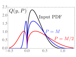
Figure 9: Twist-2 part of $Q(y,P)$ for $P=M/2$ and $P=M$ compared to the limiting PDF $f(y)=\frac{315}{32}\sqrt{y}(1-y)^{3}\theta(0<y<1)$.

Concluding this section, we repeat again that we see no reason to artificially split the $(\Lambda^{2}/P^{2})^{l}$ transverse-momentum corrections into the target-mass and higher twist terms. As we observed, the target-mass part in such a split gives a numerically very small portion. Furthermore, the only estimate we can imagine for the higher-twist terms is that they are given, like in Eq. (3.19), by appropriate $k_{\perp}$ moments of the TMD and kinematical $M^{2}$-dependent terms. The latter exactly cancel the target-mass corrections coming from the lower-twist operators. This returns us to the TMD parametrization, and the whole idea of spitting looses any sense.

Thus, the power $1/P^{2l}$ corrections reflect the transverse momentum effects only, and in the (realistic) situation when TMDs are not known, these corrections are not calculable from first principles. Furthermore, as we have seen in Sect. 3.2, the formally power-like $1/P^{2l}$ terms combine in a non-power $P$-dependence for the difference between the quasi-PDFs $Q(y,P)$ and the PDF $f(y)$, the exact form of which is again determined by the TMD. The only way to “scientifically” get rid of the transverse-momentum corrections is to reach sufficiently large values of $P$, for which the nonperturbative evolution of quasi-PDFs may be neglected.

At these large $P^{2}$, one should be able to see the perturbative $\ln P^{2}$ evolution of quasi-PDFs $Q(y,P)$. It has the same origin as the DGLAP (for Dokshitzer-Gribov-Lipatov-Altarelli-Parisi [60, 59, 61]) $\ln\mu^{2}$-dependence of the light-cone PDFs $f(x,\mu^{2})$. Strictly speaking, only when this DGLAP-related $\ln P^{2}$-dependence is observed, one may use the perturbative matching relations that convert the $\ln P^{2}$ -dependence of quasi-PDFs into the $\mu^{2}$-dependence of the light-cone PDFs.

However, the results of all available lattice quasi-PDF calculations, e.g., those of Refs. [52, 53, 54], show the features of unfinished nonperturbative evolution. The only reliable way to get rid of it is to use sufficiently large momenta $P$. In practice, this means that one should reach $P\gtrsim 2.5$ GeV. First, this is not a simple task and, second, the data at the highest achievable momentum are the least reliable.

In fact, the perturbative matching between the lattice data for $M(z_{3},P)$ and the light-cone PDFs is applicable when $z_{3}$ is small enough, like $z_{3}\lesssim 0.5$ fm. The momentum $P$ may be small, even zero. In what follows, we discuss the derivation of the perturbative matching that is used in the pseudo-PDF approach.

4 Perturbative QCD corrections at one loop

To convert $z_{3}^{2}$-dependence of the reduced pseudo-PDFs into the $\mu^{2}$-dependence of the light-cone PDFs, one should know the OPE coefficient function $C(w,z^{2}\mu^{2})$ (see Eq. (2.10)). An important fact is that the OPE can be established in the operator form, i.e. without specifying the matrix element in which the operators are embedded. One should just calculate a modification of the original bilocal operator by gluon corrections.

4.1 Link-related UV divergences

As mentioned already, switching off the light cone comes with a penalty in the form of ultraviolet divergences generated by the gauge link. It is convenient and instructive to analyze them in the Feynman gauge.

4.1.1 Link self-energy

The largest UV-related contribution comes from the self-energy correction to the gauge link (see Fig. 4). At one loop, it is given by

$$\Gamma_{\Sigma}(z)= ({i}g)^{2}\,C_{F}\,\frac{1}{2}\,\int_{0}^{1}\differential t_{1}\,\int_{0}^{1}\differential t_{2}\,z^{\mu}z^{\nu}\,D_{\mu\nu}^{c}[z_{3}(t_{2}-t_{1})]\ ,$$ (4.1)

where $D_{\mu\nu}^{c}[z_{3}(t_{2}-t_{1})]$ is the gluon propagator for the line connecting the points $t_{1}z_{3}$ and $t_{2}z_{3}$. For massless gluons, we have $D_{\mu\nu}^{c}(z)=-g_{\mu\nu}/4\pi^{2}z^{2}$, and end up with a divergent expression

$$\int_{0}^{1}\differential t_{1}\,\int_{0}^{1}\frac{\differential t_{2}}{(t_{2}-t_{1})^{2}}\,.$$ (4.2)

Though these integrals involve just dimensionless parameters $t_{1},t_{2}$, the divergence has an ultraviolet origin. As suggested by Polyakov[38], it may be regularized for spacelike $z$ by using the prescription $1/z_{3}^{2}\to 1/(z_{3}^{2}+a^{2})$ for the gluon propagator. This regularization softens the gluon propagator at distances $z_{3}\sim$ several $a$, and eliminates its singularity at $z_{3}=0$. In this respect, it is similar to the UV regularization produced by a finite lattice spacing $a_{L}$. In fact, a comparison with the gluon propagator in the lattice perturbation theory establishes a simple connection $a=a_{L}/\pi$ between these two cut-offs[62]. After the regularization, we have the expression

$$\Sigma(z_{3},a)= -g^{2}\,C_{F}\,\frac{z_{3}^{2}}{8\pi^{2}}\,\int_{0}^{1}\differential t_{1}\,\int_{0}^{1}\,\frac{\differential t_{2}}{z_{3}^{2}(t_{2}-t_{1})^{2}+a^{2}}$$ (4.3)

that clearly shows that, for a fixed $a$ the correction $\Sigma(z_{3},a)$ vanishes at $z_{3}=0$. The fact that $\Sigma(z_{3}=0,a)=0$ means that, at fixed $a$, $\Sigma$ gives no corrections to the vector current, i.e. the number of the valence quarks is not changed.

Calculating the integrals gives[62]

$$\Sigma(z_{3},a)=-\,C_{F}\,\frac{\alpha_{s}}{2\pi} \left[\,2\frac{|z_{3}|}{a}\,\tan^{-1}\left(\frac{|z_{3}|}{a}\right)-\ln\left(1+\frac{z_{3}^{2}}{a^{2}}\right)\right]\ .$$ (4.4)

If we keep $z_{3}$ fixed and take the small-$a$ limit, the result

$$\Sigma(z_{3},a)|_{a\to 0}= -\,C_{F}\,\frac{\alpha_{s}}{2\pi}\left[\,\frac{\pi|z_{3}|}{a}-2-\ln\frac{z_{3}^{2}}{a^{2}}+{\cal O}(a^{2}/z_{3}^{2})\right]\$$ (4.5)

(see also Ref. [45]) shows a linear divergence $\sim|z_{3}|/a$ in the $a\to 0$ limit. It also shows a logarithmic divergence $\ln{z_{3}^{2}}/{a^{2}}$. According to the all-order studies [39, 40, 41] of the Wilson loops renormalization, the one-loop correction (4.4) exponentiates. As a result, we get a strong damping factor for large $|z_{3}|$. In terms of the lattice spacing, it reads

$$Z_{\rm link}(z_{3},a_{L})\simeq e^{-A|z_{3}|/a_{L}}\ ,$$ (4.6)

with $A=C_{F}\pi\alpha_{s}/2\approx 2\alpha_{s}$. Taking $\alpha_{s}=0.2$ for an estimate, we get suppression by a factor of 10 starting with $z_{3}=6a_{L}$. Note also that the $Z$-factor is a function of $z_{3}/a_{L}$, i.e., it changes when the lattice spacing is changed. Hence, it is a lattice artifact, not related to actual physical phenomena in the continuum theory. As discussed already, extracting PDFs, one should divide it out. Still, it is interesting to check if the actual lattice simulations are in agreement with its perturbative estimate.

4.1.2 Vertex contribution

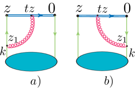
Figure 10: Insertions of gluons coming out of the gauge link.

The UV divergent contributions are also present in the diagrams involving gluons that connect the gauge link with the quarks, see Fig. 10. Regularizing the gluon propagator by $1/z_{3}^{2}\to 1/(z_{3}^{2}+a^{2})$, we extract the UV-singular term in the form

$$O^{\alpha}_{\rm UV}(z,a)= \frac{g^{2}}{4\pi^{2}}\,C_{F}\,\bar{\psi}(0)\gamma^{\alpha}\psi(0)\int_{0}^{1}d\beta\,\int_{0}^{1}\differential t\,\frac{tz_{3}^{2}}{t^{2}z_{3}^{2}+a^{2}/(1-\beta)}\,.$$ (4.7)

Taking integrals over $t$ and $\beta$ gives the expression

$$O^{\alpha}_{\rm UV}(z,a)= \frac{\alpha_{s}}{2\pi}\,C_{F}\,\bar{\psi}(0)\gamma^{\alpha}\psi(0)\left[\left(1+\frac{a^{2}}{z_{3}^{2}}\right)\,\ln\left(1+\frac{z_{3}^{2}}{a^{2}}\right)-1\right]\$$ (4.8)

that contains the same $\ln\left(1+{z_{3}^{2}}/{a^{2}}\right)$ logarithmic term as in the self-energy correction (4.4). In the $a\to 0$ limit, this result agrees with that obtained in Ref. [45]. The $\ln(1+z_{3}^{2}/a^{2})$ structure may be combined with the UV divergences generated by the link self-energy diagrams. Again, for a fixed $a$, the $O^{\alpha}_{\rm UV}(z_{3},a)$ contribution vanishes in the $z_{3}^{2}\to 0$ limit. Just like in the case of the link self-energy corrections, the UV divergences coming from vertex diagrams exponentiate in higher orders.

The UV divergent term comes from the configuration when the exchanged gluon ends coincide. The study performed in Ref. [21] shows that there is also an UV-finite contribution coming from the regions where the point $z_{1}$ is close to some position on the link. The combined contribution of two diagrams shown in Fig. 10 is given by

$$O^{\alpha}_{\rm reg}(z_{3},a=0)= \,\frac{\alpha_{s}}{2\pi}\,C_{F}\,\int_{0}^{1}du\int_{0}^{1}\differential v\,\bar{\psi}(uz_{3})\gamma^{\alpha}\psi(\bar{v}z_{3})$$

$$\times\left\{\delta(v)\left[\frac{\bar{u}}{u}\right]_{+}+\delta(u)\left[\frac{\bar{v}}{v}\right]_{+}\right\}\ .$$ (4.9)

We use the notation $\bar{v}=1-v,\bar{u}=1-u$, etc. The plus-prescription is defined by

$$\,\int_{0}^{1}du\left[\frac{\bar{u}}{u}\right]_{+}F(u)=\,\int_{0}^{1}du\,\frac{\bar{u}}{u}\,[F(u)-F[0]\ ,$$ (4.10)

assuming that $F(0)$ is finite. Now, it is the plus-prescription structure of Eq. (4.9) which guarantees that this term gives no corrections to the local current.

4.2 Evolution terms

The contributions considered in the previous section do not have singularities when the quark virtuality $k^{2}$ vanishes, i.e. they do not need any IR regularization. In particular, the logarithm $\ln(1+z_{3}^{2}/a^{2})$ has $a$ as an UV cut-off, while $z_{3}^{2}$ stays on its IR side. However, vertex diagrams also contain additional contributions that are infrared divergent in the $k^{2}\to 0$ limit.

Of course, on the lattice everything will be finite. Just like the finite lattice spacing provides a UV cut-off, the finite hadron size provides an IR cut-off. Unfortunately, the exact form of the IR regularization imposed by the hadron size is not known. To get a feeling, let us take an infrared regularization by a mass term. A typical Schwinger’s $\alpha$-parameter integral producing an IR singularity then has the form

$$L_{K}(z_{3}^{2})=\int_{0}^{\infty}\frac{d\alpha}{\alpha}e^{-z_{3}^{2}/4\alpha-\alpha m^{2}}\ ,$$ (4.11)

where $m$ is the mass (see, e.g., Ref. [21] for details). One can see that

$$L_{K}(z_{3}^{2})= 2K_{0}(mz_{3})=-\ln\left(m^{2}z_{3}^{2}\frac{e^{2\gamma_{E}}}{4}\right)+{\cal O}(z_{3}^{2})\ ,$$ (4.12)

where $K_{0}(mz_{3})$ is the modified Bessel function. It has a $\ln z_{3}^{2}$ singularity for small $z_{3}$, and exponentially decreases when $z_{3}$ exceeds $1/m$. Since we want $m$ to mimic the IR cut-off imposed by the hadron size, numerically $m$ should be of an order of 0.5 GeV. Another type of the IR regularization is provided by a sharp cut-off

$$L_{G}(z_{3}^{2})=\int_{0}^{\Lambda^{2}}\frac{d\alpha}{\alpha}e^{-z_{3}^{2}/4\alpha}=\Gamma[0,z_{3}^{2}\Lambda^{2}/4]=-\ln\left(z_{3}^{2}\Lambda^{2}\frac{e^{\gamma_{E}}}{4}\right)+{\cal O}(z_{3}^{2})\$$ (4.13)

applied to Eq. (4.11). The incomplete gamma-function $\Gamma(0,z_{3}^{2}\Lambda^{2}/4)$ has a logarithmic singularity for small $z_{3}^{2}$, while for large $z_{3}^{2}$ it has a Gaussian $e^{-z_{3}^{2}\Lambda^{2}/4}$ fall-off.

As we discussed, the UV link-related $Z$-factor also has a rapid $e^{-A|z|/a}$ decrease for large $|z|$. Thus, one needs to very precisely divide it out from the lattice data to be able to see the fall-off reflecting the finite hadron size.

For both cases, the IR-singular contribution from vertex diagrams is given[32] by

$$O^{\alpha}_{\rm log}(z_{3}) =\,L_{R}(z_{3}^{2})\,\frac{\alpha_{s}}{2\pi}\,C_{F}\,\int_{0}^{1}du\int_{0}^{1}\differential v$$

$$\times\,\left\{\delta(u)\left[\frac{\bar{v}}{v}\right]_{+}+\delta(v)\left[\frac{\bar{u}}{u}\right]_{+}\right\}\,\bar{\psi}(uz_{3})\gamma^{\alpha}\psi(\bar{v}z_{3})\ ,$$ (4.14)

where $R$ is either $K$ or $G$. One may also use the IR dimensional regularization. In the $\overline{\rm MS}$ scheme, $L_{\overline{\rm MS}}(z_{3}^{2})=-\ln\left(\mu^{2}z_{3}^{2}{e^{2\gamma_{E}}}/{4}\right)$. However, one should realize that the lattice cannot provide the dimensional IR regularization, and the data will not show the $\ln(z_{3}^{2})$ behavior beyond a few lattice spacings.

Note that, in contrast to the UV divergent contribution, the $L_{R}(z_{3}^{2}\Lambda^{2})$ functions are singular in the $z_{3}^{2}\to 0$ limit, and the parameter $|z_{3}|$ in the integrals of Eqs. (4.12), (4.13) works like an ultraviolet rather than an infra-red cut-off.

The integrals producing the IR-singular terms, also contain an IR finite part

$$O^{\alpha}_{\rm Fin}(z)= -\,\frac{\alpha_{s}}{\pi}\,C_{F}\int_{0}^{1}du\int_{0}^{1}\differential v\,\bar{\psi}(uz)\gamma^{\alpha}\psi(\bar{v}z)\left[\delta(u)\,s_{+}(v)+\delta(v)\,s_{+}(u)\right]\ ,$$ (4.15)

where $s_{+}(u)$ is the plus-prescription version of $s(u)$ given by

$$s(u) \equiv\int_{u}^{1}\differential t\,\frac{\ln t}{t^{2}}=\frac{1-u+\log(u)}{u}\ .$$ (4.16)

4.3 Quark-gluon exchange contribution

There is also an IR-singular contribution given by the diagram 11a containing a gluon exchange between two quark lines. It is given by

$$O^{0}_{\rm exch}(z_{3}) =\,\frac{\alpha_{s}}{2\pi}\,C_{F}\,\int_{0}^{1}du\int_{0}^{1-u}\differential v\,\left\{L_{R}(z_{3}^{2})\,-1\right\}\,\bar{\psi}(uz_{3})\gamma^{0}\psi(\bar{v}z_{3})\$$ (4.17)

for $R=K,G$. For DR in the $\overline{\rm MS}$ scheme, $L_{R}-1$ should be substituted by $L_{\overline{\rm MS}}+1$. Unlike the vertex part, the exchange contribution (4.17) does not have the plus-prescription form.

One should also include the quark self-energy diagrams, one of which is shown in Fig. 11b. As usual, we should take just a half of each, absorbing the other halves into the soft part. Since the quark momentum is not changed, these terms have the $\delta(u)\delta(v)$ structure in the $u,v$-integral.

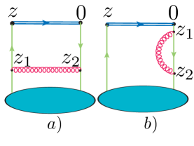
Figure 11: a) Gluon exchange diagram. b) One of quark self-energy correction diagrams.

4.4 One-loop correction in the operator form

Combining all the one-loop corrections[21] to the ${\cal O}^{0}(z_{3})$ operator gives

$$\delta {\cal O}^{0}(z_{3})=-\frac{\alpha_{s}}{2\pi}\,C_{F}\,\int_{0}^{1}du\int_{0}^{1-u}\differential v\,\bar{\psi}(uz_{3})\gamma^{0}\psi(\bar{v}z_{3})$$

$$\times\left\{\left(\delta(v)\left[\frac{\bar{u}}{u}\right]_{+}+\delta(u)\left[\frac{\bar{v}}{v}\right]_{+}+1\right)\ln\left[z_{3}^{2}\mu_{\rm IR}^{2}\frac{e^{2\gamma_{E}}}{4}\right]\right.$$

$$\left.\hskip 28.45274pt+2\left(\delta(v)\left[\frac{\ln u}{u}\right]_{+}+\delta(u)\left[\frac{\ln v}{v}\right]_{+}-1\right)\right.+Z(z_{3})\delta(u)\delta(v)\Bigr{\}}\ .$$ (4.18)

In this result, we assume the dimensional regularization and the $\overline{\rm MS}$ scheme subtraction for the IR singularities, with $\mu_{\rm IR}$ serving as the scale parameter. The function $Z(z_{3})$ accumulates information about corrections associated with the UV-divergent contributions like (4.4), (4.8). This function in the $\overline{\rm MS}$ scheme is known (see Ref. [63]), but we do not need its explicit form in the pseudo-PDF approach. As we discussed in Sec. 2.4, such terms cancel when one forms the reduced Ioffe-time pseudodistributions.

4.5 Matching for parton distribution functions

In the PDF case, the one-loop correction to ${M}^{0}(z_{3},p)$ is given by the forward matrix element $\langle p|\delta{\cal O}^{0}(z_{3})|p\rangle$. The right-hand-side of Eq. (4.18) brings then the matrix element

$$\langle p|\bar{\psi}(uz_{3})\Gamma^{0}\psi(\bar{v}z_{3})|p\rangle\equiv{\cal M}_{0}(u\nu,\bar{v}\nu)\ ,$$ (4.19)

where $\nu=p_{3}z_{3}$ is the Ioffe time [10]. The structure of Eq. (4.18) implies a scenario in which the $z_{3}^{2}$-dependence at short distances is determined by the “hard” logarithms $\ln z_{3}^{2}$ generated from the initially “soft” distribution ${\cal M}_{0}(\nu,z_{3}^{2})$ having only a polynomial dependence on $z_{3}^{2}$ that is negligible for small $z_{3}^{2}$. For this reason, we skip the $z_{3}^{2}$-dependence in the argument of ${\cal M}_{0}$-functions, leaving just their $\nu$-dependence.

The “vertex” terms containing $\delta(u)$ or $\delta(v)$ are trivially reduced to one-dimensional integrals in which we change $u$ or $v$ to $1-w$. Using translation invariance for the “box” terms having a $u,v$-independent coefficient function, we get

$$\,\int_{0}^{1}du\int_{0}^{1-u}\differential v\,{\cal M}_{0}((1-u-v)\nu)=\int_{0}^{1}\differential w\,(1-w){\cal M}_{0}(w\nu)\ .$$ (4.20)

We can represent $(1-w)$ as the sum of the term $(1-w)_{+}$ that has the plus-prescription at $w=1$ and the delta-function term $\frac{1}{2}\delta(\bar{w})$ that we add to $Z(z_{3})$, denoting the changed $Z$-function by $\widetilde{Z}(z_{3})$. As a result, we have

$${\cal M}(\nu,z_{3}^{2}) =\Biggl{[}1-\frac{\alpha_{s}}{2\pi}\,C_{F}\widetilde{Z}(z_{3})\Biggr{]}{\cal M}_{0}(\nu)-\frac{\alpha_{s}}{2\pi}\,C_{F}\,\int_{0}^{1}\differential w\,{\cal M}_{0}(w\nu)$$

$$\times\Biggl{\{}\frac{1+w^{2}}{1-w}\ln\left(z_{3}^{2}\mu_{\rm IR}^{2}\frac{e^{2\gamma_{E}+1}}{4}\right)+4\frac{\ln(1-w)}{1-w}-2(1-w)\Biggr{\}}_{+}\ .$$ (4.21)

The combination

$$B(w)= \left[\frac{1+w^{2}}{1-w}\right]_{+}\$$ (4.22)

is the non-singlet Altarelli-Parisi (AP) evolution kernel [59].

The next step is to introduce the reduced Ioffe-time pseudodistribution (2.25) of Refs. [11, 20, 17]. When the momentum $p$ is also oriented in the $z_{3}$ direction, i.e., $p=\{E,0_{\perp},p_{3}\}$, the function ${\cal M}(0,z_{3}^{2})$ corresponds to the “rest-frame” $p_{3}=0$ distribution. According to Eq. (4.21), it is given by

$${\cal M}(0,z_{3}^{2}) ={\cal M}_{0}(0)\Biggl{[}1-\frac{\alpha_{s}}{2\pi}\,C_{F}\widetilde{Z}(z_{3})\Biggr{]}\ .$$ (4.23)

As a result, the $\widetilde{Z}(z_{3})$ terms disappear from the ${\cal O}(\alpha_{s})$ correction to the ratio ${\cal M}(\nu,z_{3}^{2})/{\cal M}(0,z_{3}^{2})$. Such a cancellation of ultraviolet terms for ${\mathfrak{M}}(\nu,z_{3}^{2})$ will persist in higher $\alpha_{s}$ orders, reflecting the multiplicative renormalizability of the ultraviolet divergences[46, 45, 47] of ${\cal M}(\nu,z_{3}^{2})$.

A similar calculation can be performed for the light-cone Ioffe-time distribution[12] ${\cal I}(\nu,\mu^{2})$ obtained by taking $z^{2}=0$ in ${\mathfrak{M}}(\nu,-z^{2})$ and regularizing the resulting UV singularities by dimensional regularization and the $\overline{\rm MS}$ subtraction specified by a factorization scale $\mu$. The result may be symbolically written as

$${\cal I}(\nu,\mu^{2})={\mathfrak{M}}_{0}(\nu)- \frac{\alpha_{s}}{2\pi}\,C_{F}\,\int_{0}^{1}\differential w\,B(w)\ln\left(\mu_{\rm IR}^{2}/\mu^{2}\right){\mathfrak{M}}_{0}(w\nu)\ .$$ (4.24)

As a result, we get the matching condition[64, 21, 22, 65, 63]

$${\mathfrak{M}}(\nu,z_{3}^{2})={\cal I}(\nu, \mu^{2})-\frac{\alpha_{s}}{2\pi}\,C_{F}\,\int_{0}^{1}\differential w\,{\cal I}(w\nu,\mu^{2})\Biggl{\{}\Biggl{[}\frac{1+w^{2}}{1-w}\Biggr{]}_{+}\,$$

$$\times\ln\left(z_{3}^{2}\mu^{2}\frac{e^{2\gamma_{E}+1}}{4}\right)+4\frac{\ln(1-w)}{1-w}-2(1-w)\Biggr{\}}_{+}\$$ (4.25)

that relates ${\mathfrak{M}}(\nu,z_{3}^{2})$ with the light-cone ITD ${\cal I}(\nu,\mu^{2})$. Note that this relation works for small $z_{3}^{2}$ only, namely, in the region where the IR sensitive factors $L_{R}(z_{3}^{2})$ may be approximated by $\ln z_{3}^{2}$. In this region, ${\mathfrak{M}}(\nu,z_{3}^{2})$ satisfies the DGLAP evolution equation

$$\frac{d}{d\ln z_{3}^{2}}\,{\mathfrak{M}}(\nu,z_{3}^{2}) =-\frac{\alpha_{s}}{2\pi}\,C_{F}\int_{0}^{1}du\,B(u){\mathfrak{M}}(u\nu,z_{3}^{2})\ .$$ (4.26)

Eq. (4.25) allows to get ${\cal I}(\nu,\mu^{2})$ using lattice data on ${\mathfrak{M}}(\nu,z_{3}^{2})$. After that, inverting the Fourier transform (2.21) one should be able to get $f(x,\mu^{2})$. However, lattice calculations provide ${\mathfrak{M}}(\nu,z_{3}^{2})$ and, hence, ${\cal I}(\nu,\mu^{2})$ in a rather limited range of $\nu$, which makes taking this Fourier transform rather tricky (see Ref. [66] for a detailed discussion). An easier way was proposed in our paper [11]. The idea is to assume some parametrization for ${f}(x,\mu^{2})$ similar to those used in global fits (see, e.g., Ref. [67]), and to fit its parameters using ${\cal I}(\nu,\mu^{2})$ extracted from the lattice data through Eq. (4.25).

An equivalent realization of this idea (similar to that of Ref. [68]) is to use the kernel relation (2.23), i.e., to substitute ${\cal I}(\nu,\mu^{2})$ by its definition (2.21) as a Fourier transform of PDF. This converts (4.25) into

$${\mathfrak{M}}(\nu,z_{3}^{2})=\int_{-1}^{1}\differential x\,\left[e^{ix\nu}-\frac{\alpha_{s}}{2\pi}\,C_{F}R(x\nu,z_{3}^{2}\mu^{2})\right]\,{f}(x,\mu^{2})\ .\$$ (4.27)

The kernel $R(x\nu,z_{3}^{2}\mu^{2})$ is given by the Fourier transform (2.24) of the coefficient function, and may be calculated as a closed-form expression[63, 25].

The PDF $f(x)$ may be split in its symmetric $f^{+}(x)$ and antisymmetric $f^{-}(x)$ parts. For positive $x$, they are related to the quark $f_{q}(x)$ and antiquark $f_{\bar{q}}(x)$ distributions through $f^{+}(x)=f_{q}(x)-f_{\bar{q}}(x)$ and $f^{-}(x)=f_{q}(x)+f_{\bar{q}}(x)$, respectively (see, e.g., Ref. [17]). The real part of $R(y,z_{3}^{2}\mu^{2})$ generates then the real part of ${\mathfrak{M}}(\nu,z_{3}^{2})$ from $f^{+}(x)$, while the imaginary part of $R(y,z_{3}^{2}\mu^{2})$ connects the imaginary part of ${\mathfrak{M}}(\nu,z_{3}^{2})$ with $f^{-}(x)$. In particular, for the real part we have

$${\rm Re}\,R(\nu x,z_{3}^{2}\mu^{2})=\Biggl{\{}\frac{1-\cos(\nu x)}{\nu^{2}x^{2}}-\frac{2\sin(\nu x)}{\nu x}+2\,\sin(\nu x)\,\text{Si}(\nu x)\,$$

$$+2\,\cos(\nu x)\left(\text{Ci}(\nu x)-\log(\nu x)-\gamma_{E}+\frac{3}{4}\right)\Biggr{\}}\ln\left(z_{3}^{2}\mu^{2}\frac{e^{2\gamma_{E}+1}}{4}\right)$$

$$+2{\rm Re}\left[i\nu xe^{i\nu x}\,_{3}F_{3}(1,1,1;2,2,2;-i\nu x)\right]+\cos(\nu x)-2\,\frac{1-\cos(\nu x)}{\nu^{2}x^{2}}\,,$$ (4.28)

where $\text{Ci}(y)$ and $\text{Si}(y)$ are the integral cosine and sine functions, and ${}_{3}F_{3}(1,1,1;2,2,2;-iy)$ is a hypergeometric function. Thus, assuming some parametrizations for the $f^{\pm}(x,\mu^{2})$ distributions, one can fit their parameters and $\alpha_{s}$ using Eqs. (4.27), (4.28) and the lattice data for ${\mathfrak{M}}(\nu,z_{3}^{2})$.

Note that, despite the terms with $\nu x$ factors in their denominators, the kernel $R(\nu x,z_{3}^{2}\mu^{2})$ vanishes for $\nu x=0$. To this end, recall that, according to its definition (2.24), the kernel $R(0,z_{3}^{2}\mu^{2})$ is given by the $w$-integral of the coefficient function $C(w,z^{2}\mu^{2})$ that has the plus-prescription form in our case.

5 Exploratory quenched lattice study

5.1 General features

An exploratory lattice study of the reduced pseudo-ITD ${\mathfrak{M}}(\nu,z_{3}^{2})$ for the valence $u_{v}(x)-d_{v}(x)$ parton distribution in the nucleon has been reported in Ref. [17]. The calculations were performed in the quenched approximation on $32^{3}\times 64$ lattices, for the lattice spacing $a=0.093$ fm at the pion mass of $601(1)$ MeV and the nucleon mass of $1411(4)$MeV. Seven lattice momenta $p\,(2\pi/L)$, with $p=0,\ldots 6$ were used. The maximal momentum reached is $2.5\,$GeV. This simplified setup has allowed to get very precise data in a very short time, and its results are a very instructive illustration of applications in the theory of the pseudo-PDFs.

5.2 Rest-frame amplitude

The basic idea of the pseudo-PDF approach is to get information about the reduced pseudo-ITD. To this end, one needs to measure the ratio $R(z_{3},p_{3})=M(z_{3},p_{3})/M(z_{3},p_{3}=0)$. As we discussed, the rest-frame amplitude $M(z_{3},0)$ is basically given by the link UV-factor $Z_{\rm link}(z_{3}/a_{L})$, that exponentially decreases for large $z_{3}$ (see Eq. (4.6)). Thus, if $M(z_{3},p_{3})$ and $M(z_{3},p_{3}=0)$ are obtained from independent measurements, then the errors in the main amplitude $M(z_{3},p_{3})$ are magnified by the $1/M(z_{3},p_{3}=0)$ factor which is very large for large $z_{3}$. For this reason, in Ref. [17], the calculations were performed directly for the ratio $R(z_{3},p_{3})$ itself, rather than for the numerator and denominator independently.

However, one can also calculate the rest-frame amplitude separately, and analyze its $z_{3}$-behavior. The amplitude $M(z_{3},p_{3})$ has a real and imaginary parts. Its real part is an even function of $\nu=p_{3}z_{3}$, while the imaginary part is odd in $\nu$. Hence, the imaginary part should vanish for $p_{3}=0$. Indeed, the results for the imaginary part of $M(z_{3},p_{3}=0)$ obtained in Ref. [17] are compatible with zero. The real part was found to be a symmetric function of $z_{3}$, as expected. The results for $z_{3}\geq 0$ are displayed in Fig. 12. The curve shown there is the exponentiated version

$$Z_{\rm pert}(z_{3}/a_{L})=\exp\left\{-\,C_{F}\,\frac{\alpha_{s}}{2\pi}\left[\,2\frac{\pi|z_{3}|}{a_{L}}\,\tan^{-1}\left(\frac{\pi|z_{3}|}{a_{L}}\right)-2\ln\left(1+\frac{\pi^{2}z_{3}^{2}}{a_{L}^{2}}\right)\right]\right\}\$$ (5.1)

of the UV factors coming from the one-loop link self-energy (4.4) and vertex (4.8) corrections, in which we substituted the Polyakov regularization parameter $a$ by the lattice spacing $a_{L}$ using the correspondence $a=a_{L}/\pi$ found in Ref. [62]. The value of $\alpha_{s}$ obtained from the fit is 0.19. Thus, the “nonperturbative” renormalization factor $Z(z_{3}/a)$ in this particular lattice simulation was found to be very accurately reproduced by the perturbative formula. This fact, in our opinion, deserves a further study. Still, whatever its form, the UV $Z$-factor completely cancels out in the ratio ${\cal M}(\nu,z_{3}^{2})/{\cal M}(0,z_{3}^{2})$ defining the reduced Ioffe-time pseudodistribution.

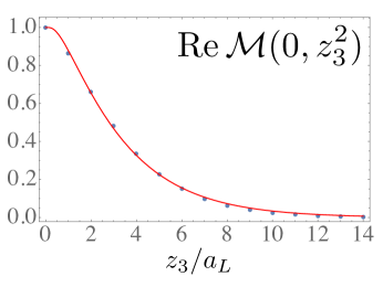
Figure 12: Real part of the rest-frame amplitude $M(z_{3},p_{3}=0)={\cal M}(0,z_{3}^{2})$.

5.3 Reduced Ioffe-time distributions

On the left panel of Fig. 13, we plot the results for the real part of the ratio ${\cal M}(Pz_{3},z_{3}^{2})/{\cal M}(0,z_{3}^{2})$ taken at six values of the momentum $P$ and plotted as a function of $z_{3}$ . One can see that the curves decrease much slower with $z_{3}$ than ${\cal M}(0,z_{3}^{2})$ of Fig. 12. The curves look similar to each other, all of them having a broad Gaussian-like shape. However, the width decreases with $P$.

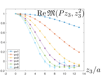
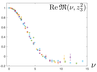
Figure 13: Left: Real part of the reduced distribution ${\mathfrak{M}}(Pz_{3},z_{3}^{2})$ plotted as a function of $z_{3}$. Here, $P=2\pi p/L$. Right: The same data plotted as a function of $\nu=Pz_{3}$.

On the right panel of Fig. 13 , we plot the same data, but change the axis to $\nu=Pz_{3}$. Now the data practically fall on the same curve. The situation is similar for the imaginary part. An evident interpretation of this outcome is that the numerator ${\cal M}(\nu,z_{3}^{2})$ and the denominator ${\cal M}(0,z_{3}^{2})$ of the ratio defining the reduced pseudo-ITD ${\mathfrak{M}}(\nu,z_{3}^{2})$ have similar dependence on $z_{3}^{2}$. In other words, the data indicate that the $z_{3}^{2}$-dependence of ${\mathfrak{M}}(\nu,z_{3}^{2})$ factorizes from its $\nu$-dependence, ${\mathfrak{M}}(\nu,z_{3}^{2})\approx{\cal I}(\nu){\mathfrak{M}}(0,z_{3}^{2})$.

Still, one can also notice some apparently random scatter of the points corresponding to the same value of $\nu$. In fact, there is a regularity in this scatter. On the left panel of Fig. 14, we show the data corresponding to “large” $z_{3}$-values: from $7a_{L}$ to $14a_{L}$. As one can see, there is some scatter for the points with the largest values of $\nu$ in the region $\nu\gtrsim 10$, where the finite-volume effects become important.

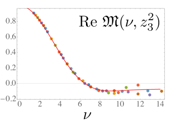
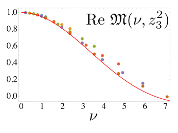
Figure 14: Real part of ${\mathfrak{M}}(\nu,z_{3}^{2})$ for $z_{3}$ ranging from $7a_{L}$ to $14a_{L}$ (left) and from $a_{l}$ to $6a_{L}$ (right).

Otherwise, practically all the points lie on the curve

$${\cal R}(\nu)= \int_{0}^{1}\differential x\,\cos(\nu x)\,f_{v}(x)$$ (5.2)

generated by the function

$$f_{v}(x)=\frac{315}{32}\sqrt{x}(1-x)^{3}\,.$$ (5.3)

Its shape was obtained by taking normalized $x^{a}(1-x)^{b}$-type functions and fixing the parameters $a,b$ by fitting the data.

Recall that the real part of the light-cone ITD ${\cal I}(\nu)$ corresponds to the cosine Fourier transform of the valence distribution $q_{v}(x)=u_{v}(x)-d_{v}(x)$

$${\cal I}_{R}(\nu)\equiv{\rm Re}\,{\cal I}(\nu)= \int_{0}^{1}\differential x\,\cos(\nu x)\,q_{v}(x)\ .$$ (5.4)

On the right panel of Fig. 14, we show the points in the region of “small” $z_{3}$, ranging in the interval $a_{L}\leq z_{3}\leq 6a_{L}$. In this case, all the points lie higher than the curve for $R(\nu)$. Since ${\mathfrak{M}}(\nu,z_{3}^{2})$, according to Eq. (4.25), contains the evolution logarithm $\ln z_{3}^{2}$ in the region of small $z_{3}^{2}$, one may conjecture that the observed higher values of ${\rm Re}\,{\mathfrak{M}}$ for smaller-$z_{3}$ points may be a consequence of the evolution.

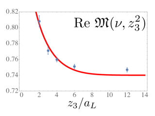
Figure 15: Dependence on $z_{3}$ for $\nu=3\pi/4\approx 2.3562$.

In Fig. 15 we show a typical pattern of the $z_{3}$-dependence of the lattice points. We took there the “magic” Ioffe-time value $\nu=3\pi/4$ that may be obtained from five different combinations of $z_{3}$ and $P$ values used in Ref. [17]. The shape of the eye-ball fit line is given by the incomplete gamma-function $\Gamma(0,z_{3}^{2}/30a_{L}^{2})$. This function conforms to our expectation that the $z_{3}$-dependence of the IR-sensitive factors $L_{R}(z_{3})$ in (4.14), (4.17) should have a perturbative logarithmic $\ln(1/z_{3}^{2})$ behaviour for small $z_{3}$, and rapidly vanish for $z_{3}$ larger than the hadron size $R_{\rm hadr}$. We can estimate that $R_{\rm hadr}$ in this lattice simulation is of an order of $6a_{L}\approx 0.55$ fm. Looking at Fig. 15, we may also say that perturbative evolution “stops” for $z_{3}\gtrsim 5a_{L}$. In this sense, the overall curve based on Eq. (5.3) corresponds to a “low normalization point”, i.e., to the region, where the perturbative evolution is absent.

5.4 Building $\overline{\rm MS}$ ITD

Thus, we see that the data of Fig. 15 show a logarithmic evolution behavior in the small $z_{3}$ region. Still, the $z_{3}$-behavior starts to visibly deviate from a pure logarithmic $\ln z_{3}^{2}$ pattern for $z_{3}\gtrsim 5a$. Thus, $z_{3}\leq 4a$ is the “logarithmic region” where one may use Eq. (4.25) to construct the light-cone $\overline{\rm MS}$ ITD. To this end, it is convenient to invert it and write

$${\cal I}(\nu, \mu^{2})={\mathfrak{M}}(\nu,z_{3}^{2})+\frac{\alpha_{s}}{2\pi}\,C_{F}\,\int_{0}^{1}\differential w\,{\mathfrak{M}}(w\nu,z_{3}^{2})$$

$$\times\Biggl{\{}\Biggl{[}\frac{1+w^{2}}{1-w}\Biggr{]}_{+}\,\ln\left(z_{3}^{2}\mu^{2}\frac{e^{2\gamma_{E}+1}}{4}\right)+4\frac{\ln(1-w)}{1-w}-2(1-w)\Biggr{\}}_{+}\ .\$$ (5.5)

Let us start with the real part of this relation. At the leading order in $\alpha_{s}$, we have ${\cal I}_{R}(\nu,\mu^{2})={\rm Re}\ {\mathfrak{M}}(\nu,z_{3}^{2})$. In its turn, ${\rm Re}\ {\mathfrak{M}}(\nu,z_{3}^{2})$ is given by ${\cal R}(\nu)$ of Eq. (5.2) plus scatter, which we intend to describe by the $\ln z_{3}^{2}$ part of the ${\cal O}(\alpha_{s})$ correction. This means that we should approximate ${\rm Re}\,{\mathfrak{M}}(w\nu,z_{3}^{2})$ by ${\cal R}(w\nu)$ in the ${\cal O}(\alpha_{s})$ term. Using further the definition (5.2) of $R(\nu)$ in terms of $f_{v}(x)$ given by (5.3) we get

$${\cal I}_{R}(\nu, \mu^{2})={\rm Re}\,{\mathfrak{M}}(\nu,z_{3}^{2})+\frac{\alpha_{s}}{2\pi}\,C_{F}\,\int_{0}^{1}\differential x\,f_{v}(x)\,{\rm Re}\,R(x\nu,z_{3}^{2})\ ,\$$ (5.6)

where ${\rm Re}\,R(x\nu,z_{3}^{2})$ is the kernel specified by Eq. (4.28).

The next step is to check if the actual $z_{3}^{2}$-dependence of the data on ${\mathfrak{M}}(\nu,z_{3}^{2})$ plus the $\ln z_{3}^{2}$-dependence of the one-loop correction produce together the result that has no (or little) $z_{3}^{2}$-dependence. In the worst case scenario, this will not happen for any value of $\alpha_{s}$, the only free parameter that we have. This will mean that our data are simply inconsistent with the DGLAP evolution equation.

Fortunately, as it was found in the original paper [17], the $z_{3}^{2}$-dependence of the data matches $\ln z_{3}^{2}$-dependence of the one-loop correction if one takes $\alpha_{s}/\pi=0.1$. Using this value in Eq. (5.6) and the data on ${\rm Re}\ {\mathfrak{M}}(\nu,z_{3}^{2})$, one can generate the “data points” for ${\cal I}_{R}(\nu,\mu^{2})$. This was done in Ref. [22] for $\mu=1/a_{L}$ that corresponds to $\mu=2.15$ GeV. The results are shown in the left panel of Fig. 16.

     

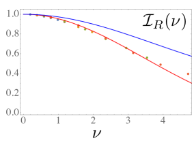
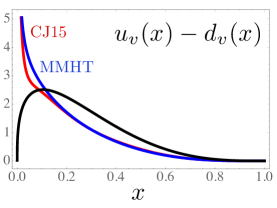
Figure 16: Left: Function ${\cal I}_{R}(\nu,\mu^{2})$ for $\mu=1/a_{L}$ calculated using the data with $z_{3}$ from $a_{L}$ to $4a_{L}$. The upper curve corresponds to the ITD of the CJ15 global fit PDF. Right: Curve for $u_{v}(x)-d_{v}(x)$ at $\mu=2.15$ GeV built from the data shown on the left compared to CJ15 and MMHT global fits.

One can see that all the points for ${\cal I}_{R}(\nu,\mu^{2})$ are close to some universal curve with a rather small scatter. The curve itself was obtained by fitting the points by the cosine transform of a normalized $Nx^{a}(1-x)^{b}$ distribution, which gave $a=0.35$ and $b=3$. The magnitude of the scatter illustrates the error of the fit for the ITD in the $\nu\leq 4$ region. For comparison, we show the ITD obtained from the global fit PDFs corresponding to the CJ15 global fit.[67] One can see that our ITD is systematically below the curve based on the global fit PDFs.

The “mathematical” reason for the discrepancy may be understood from the right panel of Fig. 16, where we compare the normalized $Nx^{0.35}(1-x)^{3}$ $\equiv q_{v}(x,\mu=2.15$ GeV) distribution to CJ15 [67] and MMHT 2014 [69] global fit PDFs, taken at the scale $\mu=2.15$ GeV. Unlike the $\sim x^{0.35}$ function, these PDFs are singular for small $x$, which leads to the enhancement of ITDs for large and moderate values of $\nu$.

The singular small-$x$ behavior of the global fit PDFs reflects the Regge dynamics, in particular, the parameters of the $\rho$-trajectory. Since the $\rho$-meson may be treated as a resonance in the two-pion system, a possible “physical” reason for the discrepancy lies in the simplified features of the lattice simulation used in Ref. [17]: the quenched approximation and very large pion mass.

5.5 Imaginary part

Imaginary part of the pseudo-ITD may be considered in a similar way. It corresponds to the sine Fourier transform

$${\rm Im}\,{\mathfrak{M}}(\nu)= \int_{0}^{1}\differential x\,\sin(\nu x)\,[q(x)+\bar{q}(x)]$$ (5.7)

of the function given by the sum $q(x)+\bar{q}(x)$ of quark and antiquark distributions. This function differs from the valence combination $q_{v}(x)=q(x)-\bar{q}(x)$ by $2\bar{q}(x)=2[\bar{u}(x)-\bar{d}(x)]$. In the left panel of Fig. 17, we show the data for large $z_{3}$ values $z_{3}\geq 7a$. Just like in the case of the real part (see Fig. 14), the points with $\nu\lesssim 10$ are close to a universal curve. Representing $q(x)+\bar{q}(x)=q_{v}(x)+2\bar{q}(x)$ and taking $f(x)$ of Eq. (5.3) as $q_{v}(x)$, the difference is fitted to be given by

$$\bar{q}(x)\approx 0.1\,[20x\,(1-x)^{3}]\,.$$ (5.8)

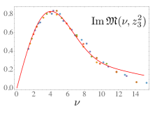
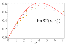
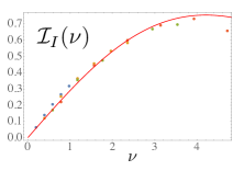
Figure 17: Left: Imaginary part of ${\mathfrak{M}}(\nu,z_{3}^{2})$ for $z_{3}$ ranging from $7a_{L}$ to $13a_{L}$. Middle: The same for $z_{3}$ from $a_{L}$ to $4a_{L}$. In both cases, the curve corresponds to $q(x)+\bar{q}(x)=f_{v}(x)+2\bar{q}(x)$, with $f_{v}(x)$ given by Eq. (5.3) and $\bar{q}(x)$ given by Eq. (5.8). Right: Function ${\cal I}_{I}(\nu,\mu^{2})$ for $\mu=1/a_{L}$ calculated using the data with $z_{3}\leq 4a$. The curve is described in the text.

In the middle panel of Fig. 17, we show data with $z_{3}\leq 4a$. All these points are below the curve obtained by fitting the $z_{3}\geq 7a$ data. This is in agreement with the fact that, in the region $\nu\lesssim 6$, the perturbative evolution decreases the imaginary part of the pseudo-ITD when $z_{3}$ decreases. The construction of the $\overline{\rm MS}$ function ${\rm Im}\,{\cal I}(\nu,\mu^{2})\equiv{\cal I}_{I}(\nu,\mu^{2})$ proceeds in the same way as for the real part.

The results are shown in the right panel of Fig. 17. Again, all the points are rather close to a universal curve with a rather small scatter. The curve shown corresponds to the sine Fourier transform of the sum of the valence distribution $q_{v}(x,\mu=1/a_{L})$ obtained from the study of the real part, and the antiquark contribution $2\bar{q}(x,\mu=1/a_{L}$). The latter was found from the fit to be given by $\bar{q}(x,\mu=1/a_{L}=2.15$ GeV$)=0.07[20x(1-x)^{3}]$.

Note that the result for $\bar{q}(x)$ is a positive function of $x$, which means that $\bar{u}(x)>\bar{d}(x)$ in the lattice simulation of Ref. [17]. For the quenched approximation, this is a natural outcome: in the absence of quark loops, the ratio $\bar{u}/\bar{d}$ reflects the number of the $u$- and $d$-quarks in the proton.

6 Calculation with dynamical fermions

A calculation with dynamical fermions was reported in Ref. [23]. The analysis was performed using three lattice ensembles for a pion mass of about 400 MeV. Two lattice spacings have been used. For the lattice spacings $a=$ 0.127 fm, the calculations have been performed on $24^{3}\times 64$ and $32^{3}\times 96$ lattices. For a smaller lattice spacing of 0.94 fm, a $32^{3}\times 64$ lattice was used. All three ensembles have produced similar results, perfectly compatible between themselves.

The dynamical calculations are more time-consuming and noisy compared to the quenched calculations, so the results have bigger statistical errors than those of Ref. [17]. Still, the structure of the pseudo-ITDs in both calculations is very similar, and their analysis follows the same steps.

6.1 Rest-frame amplitude

As discussed earlier in Sec. 2.4, 4.1, 5.2, the rest-frame amplitude ${\cal M}(0,z_{3}^{2})$ within the pseudo-PDF approach plays the role of the UV-renormalization $Z$-factor. In Fig. 18, we show the results for two explored lattice spacings of 0.094 fm and 0.127 fm. In the latter case, we show the points for a bigger $32^{2}\times 96$ lattice. The results obtained on a smaller $24^{3}\times 64$ lattice practically coincide with them. Just like in the quenched calculation, these points are well described by the perturbative formula (5.1) (shown by a curve in Fig. 18), but now with the value of 0.26 for the $\alpha_{s}$.

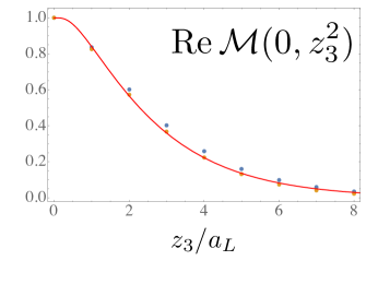
Figure 18: Real part of the rest-frame amplitude ${\cal M}(0,z_{3}^{2})$ for lattice spacings 0.094 fm (higher points) and 0.127 fm.

Note that the points for the two different lattice spacings are plotted as functions of the ratio $z_{3}/a_{L}$ rather than versus the physical distance $z_{3}$. Such a choice is suggested by the perturbative calculation that shows that the $Z$-factor should be a function of $z/a_{L}$. Indeed, one can see that the two sets of points in Fig. 18 are very close to each other. The points corresponding to the 0.094 fm lattice spacing are just slightly above the curve in Fig. 18 describing the 0.127 fm points. In fact, the 0.094 fm points are also well described by the perturbative formula (5.1), if one uses a smaller value $\alpha_{s}=0.24$.

The fact that the $Z$-factor was found to be given by a function of $z_{3}/a_{L}$ (modulo a natural change of $\alpha_{s}$ to a smaller value in the case of a smaller lattice spacing) is a clear demonstration that it is an artifact of the lattice calculation rather than a function describing physical effects.

6.2 Reduced Ioffe-time distributions

The data on the reduced pseudo-ITD are shown in Fig. 19 for the lattice spacing 0.094 fm (left) and for 0.127 fm on the large $32^{3}\times 96$ lattice (right). The curves in both cases correspond to $e^{-0.05\nu^{2}}$, and were drawn to demonstrate that the results in both cases are rather similar. The data on ${\mathfrak{M}}(\nu,z_{3}^{2})$ have been used to obtain the light-cone ITD ${\cal I}(\nu,\mu^{2})$ at the scale $\mu=2$ GeV using a technique similar to that described in Sec. 5.3.

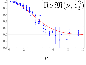
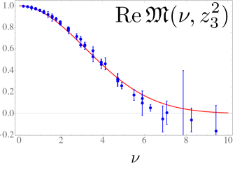
Figure 19: Real part of ${\mathfrak{M}}(\nu,z_{3}^{2})$ for lattice spacing 0.094 fm (left) and 0.127 fm (right).

The function ${\cal I}(\nu,\mu^{2})$ is plotted on the left panel of Fig. 20. The light-cone PDF $q_{v}(x)=u_{v}(x)-d_{v}(x)$ extracted from this ${\cal I}(\nu,\mu^{2})$ is shown on the right panel. The central line for the result of this calculation with dynamical fermions is in a much better agreement with phenomenological curves. Still, the error band is very wide, which calls for a simulation having a better statistics.

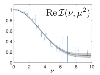
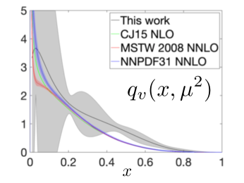
Figure 20: Real part of the light-cone ITD ${\cal I}(\nu,\mu^{2})$ (left) and the valence PDF $q_{v}(x,\mu^{2})$ (right) for $\mu=2$ GeV extracted from the data for lattice spacing 0.094 fm.

6.3 Moments

The basic matching relation (4.25) has a $w$-convolution structure in its ${\cal O}(\alpha_{s})$ part. However, it may be converted into a product form if one considers the $x^{n}$ moments

$$b_{n}(z_{3}^{2})\equiv\int_{0}^{1}\differential xx^{n}{\mathfrak{P}}(x,z_{3}^{2})=\left.i^{n}\frac{\partial^{n}\,{\mathfrak{M}}(\nu,z_{3}^{2})}{\partial\nu^{n}}\right|_{\nu=0}\$$ (6.1)

of the renormalized pseudo-PDF ${\mathfrak{P}}(x,z_{3}^{2})\equiv{\cal P}(x,z_{3}^{2})/{\cal M}(0,z_{3}^{2})$. This gives

$$b_{n}(z_{3}^{2})=K_{n}(z_{3}^{2}\mu^{2})a_{n}(\mu^{2})+{\cal O}(z_{3}^{2}\Lambda^{2}_{\rm QCD},\alpha_{s}^{2})\ ,$$ (6.2)

a connection between $b_{n}(z_{3}^{2})$ and the $x^{n}$ moments

$$a_{n}(\mu^{2})=\int_{0}^{1}\differential xx^{n}{f}(x,\mu^{2})\$$ (6.3)

of the light-cone PDF $f(x,\mu^{2})$. The kernel $K_{n}(z_{3}^{2}\mu^{2})$ is given by[23]

$$K_{n}(z^{2}\mu^{2},\alpha_{s})=1-\frac{\alpha_{s}}{2\pi}C_{F}\left[\gamma_{n}\ln\left(z^{2}\mu^{2}\frac{e^{2\gamma_{E}+1}}{4}\right)+l_{n}\right]\,,$$ (6.4)

where the anomalous dimensions

$$\gamma_{n}=\int_{0}^{1}\differential u\,B(u)u^{n}=\frac{1}{(n+1)(n+2)}-\frac{1}{2}-2\sum_{k=2}^{n+1}\frac{1}{k}$$ (6.5)

are the moments of the Altarelli-Parisi kernel $B(u)$, and the coefficients

$$l_{n}=2\left[\left(\sum_{k=1}^{n}\frac{1}{k}\right)^{2}+\sum_{k=1}^{n}\frac{1}{k^{2}}+\frac{1}{2}-\frac{1}{(n+1)(n+2)}\right]$$ (6.6)

are the moments of the remaining terms in the second line of Eq. (4.25). Thus, one can now obtain the $\overline{\rm MS}$ moments directly from the reduced ITD ${\mathfrak{M}}(\nu,z^{2})$ by using

$$a_{n}(\mu^{2})=(-i)^{n}\frac{1}{K_{n}(z_{3}^{2}\mu^{2},\alpha_{s})}\left.\frac{\partial^{n}\,{\mathfrak{M}}(\nu,z^{2})}{\partial\nu^{n}}\right|_{\nu=0}+O(z_{3}^{2}\Lambda^{2}_{\rm QCD},\alpha_{s}^{2})\,.$$ (6.7)

The first moment $a_{1}\equiv\langle x\rangle$ is obtained from the slope of the imaginary part of ${\mathfrak{M}}(\nu,z^{2})$, while $a_{2}\equiv\langle x^{2}\rangle$ from the $\nu^{2}$-fit of the real part. The results for $\langle x\rangle$ and $\langle x^{2}\rangle$ obtained from all three ensembles are presented in Ref. [27]. In Fig. 21, we show the results for $\langle x^{2}\rangle$ from the 0.094 fm ensemble.

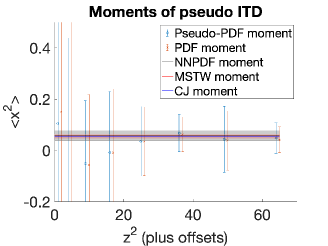
Figure 21: The $\langle x^{2}\rangle$ moment of the pseudo-PDF obtained from the 0.094 fm ensemble and compared to phenomenologically determined PDF moments from the NLO global fit CJ15nlo [67], and the NNLO global fits MSTW2008nnlo68cl_nf4 [70] and NNPDF31_nnlo_pch_as_0118_mc_164 [71], all evolved to 2 GeV.

7 Matching in nonforward kinematics

The matching relations (4.25) for PDFs were derived from the operator expression (4.18) for the one-loop correction by inserting it into a forward matrix element $\langle p|\ldots|p\rangle$. The same expression (4.18) may be used to deal with nonforward matrix elements[25]. In the simplest case, we have the $\langle 0|\ldots|p\rangle$ matrix element corresponding to the pion distribution amplitude. A more complicated case is the matrix element $\langle p_{2}|\ldots|p_{1}\rangle$ corresponding to a non-singlet generalized parton distribution (GPD).

7.1 Matching relation for the pion distribution amplitude

Within a framework of covariant quantum field theory, the pion distribution amplitude was introduced in our 1977 paper (see Ref. [6]). The starting point of the definition is the matrix element

$$M^{\alpha}(z,p)=\langle 0|\bar{\psi}(0)\,\gamma^{\alpha}\,\gamma_{5}{\hat{E}}(0,z;A)\psi(z)|p\rangle\ ,$$ (7.1)

with $z$ taken on the light cone. Here, $|p\rangle$ is a pion state with momentum $p$. In Ref. [72], a similar object was introduced within the light-front quantization formalism (see Ref. [73] for comparison of the two definitions).

For lattice applications, we take $z=z_{3}$ and the $\alpha=0$ component to eliminate the $z^{\alpha}$ contamination from the decomposition of $M^{\alpha}(z,p)$ over Lorentz structures and extract the $p^{\alpha}{\cal M}(\nu,-z^{2})$ part. The reduced Ioffe-time distribution is built through ${\mathfrak{M}}(\nu,z_{3}^{2})={\cal M}(\nu,z_{3}^{2})/{\cal M}(0,z_{3}^{2})$.

As shown in Ref. [13], for all contributing Feynman diagrams we have

$${\cal M}(\nu,z_{3}^{2}) =\int_{0}^{1}\differential x\,e^{ix\nu}\,{\cal F}(x,z_{3}^{2})\ .$$ (7.2)

The function ${\cal F}(x,z_{3}^{2})$ is the pion pseudodistribution amplitude (pseudo-DA). Similarly to pseudo-PDFs, we get a covariantly defined variable $x$, having in this case the $0\leq x\leq 1$ support. To exploit the symmetry properties of ${\cal F}(x,z_{3}^{2})$ with respect to the $x\to 1-x$ interchange, it is convenient to use the $(-z/2,z/2)$ endpoints instead of $(0,z)$. The relation between the two cases is provided by translation invariance,

$$\widetilde{\cal M}(\nu,z_{3}^{2})\equiv\langle 0|\bar{\psi}(-z_{3}/2)\,\ldots\psi(z_{3}/2)|p\rangle =e^{-i\nu/2}{\cal M}(\nu,z_{3}^{2})\ .$$ (7.3)

Using explicit form (4.18) of the one-loop correction, (4.18) and parametrizing

$$\langle 0|\bar{\psi}(uz_{3})\, \ldots\psi(\bar{v}z_{3})|p\rangle=e^{iu\nu}{\cal M}_{0}[(1-u-v)\nu]\ ,\$$ (7.4)

one may derive the matching condition for the pion DA[25]

$$\widetilde{\mathfrak{M}}(\nu,z_{3}^{2})=\widetilde{\mathcal{I}}(\nu,\mu^{2})-\frac{\alpha_{s}}{2\pi}\,C_{F}\,\int_{0}^{1}\differential w\,\widetilde{\mathcal{I}}(w\nu,\mu^{2})$$

$$\times\Biggl{\{}\ln\left[z_{3}^{2}\mu^{2}\frac{e^{2\gamma_{E}+1}}{4}\right]\Biggr{(}\Biggl{[}\frac{2w}{1-w}\Biggr{]}_{+}\,\cos(\bar{w}\nu/2)+\frac{\sin(\bar{w}\nu/2)}{\nu/2}-\frac{1}{2}\delta(\bar{w})\Biggr{)}$$

$$+4\Biggl{[}\frac{\ln(1-w)}{1-w}\Biggr{]}_{+}\cos(\bar{w}\nu/2)-2\frac{\sin(\bar{w}\nu/2)}{\nu/2}+\delta(\bar{w})\Biggr{\}}\ .$$ (7.5)

We use here the “tilded” light-cone ITD $\widetilde{\cal I}(\nu,\mu^{2})$ corresponding to the $(-z/2,z/2)$ endpoints. It is related to the light-cone pion DA $\Phi(x,\mu^{2})$ by

$$\widetilde{\cal I}(\nu,\mu^{2}) =\int_{0}^{1}\differential x\,e^{i(x-1/2)\nu}\,\Phi(x,\mu^{2})\ .$$ (7.6)

Thus, if $\Phi(x,\mu^{2})$ is even (odd) with respect to the $x\to 1-x$ interchange, then $\widetilde{\cal I}(\nu,\mu^{2})$ is even (odd) function of $\nu$.

To extract $\Phi(x,\mu^{2})$, we recommend, just like in the PDF case, to assume some parametrization for it, say, $N(x\bar{x})^{a}$ times some polynomial of $x$, and then to fit the parameters of the model by $\widetilde{\cal I}(\nu,\mu^{2})$ extracted from the lattice data. Another way is to use a kernel relation, analogous to Eq. (4.27), which expresses $\widetilde{\mathfrak{M}}(\nu,z_{3}^{2})$ in terms of $\Phi(x,\mu^{2})$. It is straightforward to calculate the analog of the $R(x\nu,z_{3}^{2}\mu^{2})$ in a closed form. The further procedure is to fit $\alpha_{s}$ and the parameters of the model for the light-cone DA $\Phi(x,\mu^{2})$ using the lattice data for the reduced pseudo-DA $\widetilde{\mathfrak{M}}(\nu,z_{3}^{2})$.

7.2 Definitions and kinematics of GPDs

In the case of GPDs, we should consider a nonforward matrix element $\langle p_{2}|\ldots|p_{1}\rangle$ involving hadronic states with two different momenta. The simplest case is the pion. It has just one light-cone GPD $H(x,\xi,t;\mu^{2})$ that may be defined[8] by

$$\langle p_{2}| \bar{\psi}(-z/2)\gamma^{\alpha}\hat{E}(-z/2,z/2;A)\psi(z/2)|p_{1}\rangle$$

$$=2{\cal P}^{\alpha}\int_{-1}^{1}\differential x\,e^{-ix({\cal P}z)}\,H(x,\xi,t;\mu^{2})\ ,\,\$$ (7.7)

(see also Refs. [7, 9]), where the coordinate $z$ has only the $z_{-}$ light-cone component and the choice $\alpha=+$ is made to eliminate the $z^{\alpha}$ part. As usual, $\mu$ is the factorization scale. Note that this definition involves the $(-z/2,z/2)$ endpoints, which simplifies the analysis of the $x\to-x$ symmetry properties of $H(x,\xi,t;\mu^{2})$.

The momentum ${\cal P}=(p_{1}+p_{2})/2$ here is the average of the hadron momenta. The skewness variable $\xi$ is related to the plus-component of their difference $p_{1}-p_{2}\equiv r$. Namely, $\xi=r^{+}/2{\cal P}^{+}$. One more variable is given by the invariant momentum transfer $t=(p_{1}-p_{2})^{2}$. In principle, the right-hand side of Eq. (7.7) may have also the $r^{\alpha}$ term. However, when we take $\alpha=+$, such a term is redundant, since $r^{+}=2\xi{\cal P}^{+}$.

A similar definition holds for the spin non-flip GPD $H(x,\xi,t;z^{2})$ of the nucleon. One should just substitute $2{\cal P}^{+}$ by $\bar{u}(p_{2})\gamma^{+}u(p_{1})$.

For a general case, the skewness $\xi$ may be defined as

$$\xi=\frac{(p_{1}z)-(p_{2}z)}{(p_{1}z)+(p_{2}z)}\ .$$ (7.8)

Thus, we deal with two Ioffe-time invariants $\nu_{1}\equiv-(p_{1}z)$ and $\nu_{2}\equiv-(p_{2}z)$. For lattice applications, we choose $z=z_{3}$. Decomposing $p_{1}=\{E_{1},\Delta_{1,\perp},P_{1}\}$ and $p_{2}=\{E_{2},\Delta_{2,\perp},P_{2}\}$, we have $\nu_{1}=P_{1}z_{3}$ and $\nu_{2}=P_{2}z_{3}$. The skewness variable is given by

$$\xi= \frac{\nu_{1}-\nu_{2}}{\nu_{1}+\nu_{2}}=\frac{P_{1}-P_{2}}{P_{1}+P_{2}}\,\,.\$$ (7.9)

Using the $\xi$-definition (7.9), we may write $P_{1}=(1+\xi)P$ and $P_{2}=(1-\xi)P$, where $P\equiv{\cal P}_{3}$.

Again, we choose $\alpha=0$ to eliminate the $z^{\alpha}$ part from the parametrization of $\langle p_{2}|\bar{\psi}(-z/2)\gamma^{\alpha}\hat{E}(-z/2,z/2;A)\psi(z/2)|p_{1}\rangle$ for $z=z_{3}$. Note that the $\Delta_{\perp}^{\alpha}$ contributions will be also absent in the parametrization. Hence, we can define the double Ioffe-time pseudodistribution $\widetilde{M}(\nu_{1},\nu_{2},t;z_{3}^{2})$

$$\langle p_{2}|\bar{\psi}(-z_{3}/2)\gamma^{0}\ldots\psi(z_{3}/2)|p_{1}\rangle=2{\cal P}^{0}\widetilde{M}(\nu_{1},\nu_{2},t;z_{3}^{2})\,.\$$ (7.10)

We use here the “tilde” notation indicating that $\widetilde{M}(\nu_{1},\nu_{2},t;z_{3}^{2})$ parametrizes the operator with the $(-z_{3}/2,z_{3}/2)$ endpoints. Denoting $\nu=(\nu_{1}+\nu_{2})/2$, we define the generalized Ioffe-time pseudodistribution (pseudo-GITD) by

$$\widetilde{M}(\nu_{1},\nu_{2},t;z_{3}^{2})=\widetilde{\cal M}(\nu,\xi,t;z_{3}^{2})\ .$$ (7.11)

It is related to the pseudo-GPD by

$$\widetilde{\cal M}(\nu,\xi,t;z_{3}^{2})=e^{i\xi\nu}\,\int_{-1}^{1}\differential x\,e^{ix\nu}\,{\cal H}\left(x,\xi,t;z_{3}^{2}\right)\,.\$$ (7.12)

Using the operator expression (4.18) for the one-loop contribution gives the matching relation for GPDs

$$\widetilde{\mathfrak{M}}(\nu,\xi,t,z_{3}^{2})=\widetilde{\mathcal{I}}(\nu,\xi,t,\mu^{2})-\frac{\alpha_{s}}{2\pi}\,C_{F}\,\int_{0}^{1}\differential w\,\widetilde{\mathcal{I}}(w\nu,\xi,t,\mu^{2})$$

$$\times\Biggl{\{}\ln\left[z_{3}^{2}\mu^{2}\frac{e^{2\gamma_{E}+1}}{4}\right]\Biggr{(}\Biggl{[}\frac{2w}{1-w}\Biggr{]}_{+}\,\cos(\bar{w}\xi\nu)+\frac{\sin(\bar{w}\xi\nu)}{\xi\nu}-\frac{1}{2}\delta(\bar{w})\Biggr{)}$$

$$+4\Biggl{[}\frac{\ln(1-w)}{1-w}\Biggr{]}_{+}\cos(\bar{w}\xi\nu)-2\frac{\sin(\bar{w}\xi\nu)}{\xi\nu}+\delta(\bar{w})\Biggr{\}}\ \ .$$ (7.13)

Its structure is similar to the matching relation (7.5) for the pion DA. Eq. (7.13) relates the reduced pseudo-GITD

$$\widetilde{\mathfrak{M}}(\nu,\xi,t,z_{3}^{2})\equiv\frac{\widetilde{\cal M}(\nu,\xi,t,z_{3}^{2})}{\widetilde{\cal M}(0,0,0,z_{3}^{2})}\ .$$ (7.14)

with the light-cone GITD

$$\widetilde{\mathcal{I}}(\nu,\xi,t,\mu^{2})=\int_{-1}^{1}\differential x\,e^{ix\nu}H(x,\xi,t;\mu^{2})\ .$$ (7.15)

We propose again to extract $H(x,\xi,t;\mu^{2})$ by taking some parametrization for it, and then to fit its parameters by using the lattice data on $\widetilde{\mathfrak{M}}(\nu,\xi,t,z_{3}^{2})$. Building the model, one should take into account the polynomiality property [8, 7, 9] of GPDs, i.e., the requirement that, in the non-singlet case, the $x^{N}$ moment of $H(x,\xi,t;\mu^{2})$ should be a polynomial of the $N$th degree in $\xi$. An efficient way to satisfy this requirement is to use the double distribution Ansatz [74].

Another (but equivalent) strategy is to convert (7.13) into a kernel relation. It is obtained by writing the light-cone GITD $\widetilde{\mathcal{I}}(\nu,\xi,t,\mu^{2})$ in terms of $H(x,\xi,t;\mu^{2})$ using Eq. (7.15). The kernel relation allows then to fit the parameters of $H(x,\xi,t;\mu^{2})$ from the lattice data on $\widetilde{\mathfrak{M}}(\nu,\xi,t,z_{3}^{2})$.

7.3 Lattice implementation

Lattice measurements involve a discrete set of values both for coordinates $z_{3}=n_{z}a$ and for longitudinal momenta $P_{1}=2\pi N_{1}/L$, $P_{2}=2\pi N_{2}/L$, where $L=na$ is the lattice size in the $z_{3}$ direction. Hence, possible values of the Ioffe-time parameters are given by discrete sets $\nu_{1}=2\pi n_{z}N_{1}/n$ and $\nu_{2}=2\pi n_{z}N_{2}/n$. As a result, possible values for skewness are given by rational numbers

$$\xi=\frac{P_{1}-P_{2}}{P_{1}+P_{2}}=\frac{N_{1}-N_{2}}{N_{1}+N_{2}}\ .$$ (7.16)

Changing $N_{1}$ and $N_{2}$ from 0 to 6, one ends up with 13 possible values for $\xi$. They range from 0 to 1 and represent rather well the whole $0\leq\xi\leq 1$ segment. A complication is that, varying the skewness $\xi$, one also changes the value of the momentum transfer $t$. For given $\xi$, the momentum transfer has its minimal value $t_{0}$ that is achieved for purely longitudinal initial and final momenta,

$${t_{0}}= -\frac{8\xi^{2}{M^{2}}}{1-\xi^{2}+{M^{2}}/{P^{2}}+\sqrt{(1-\xi^{2}+{M^{2}}/{P^{2}})^{2}+4\xi^{2}{M^{2}}/{P^{2}}}}\ .$$ (7.17)

To relax the correlation between the values of $t$ and $\xi$, one may add a transverse component $\Delta_{\perp}$ to the momentum transfer. In particular, taking $p_{1}=\{E_{1},\Delta_{\perp},P_{1}\}$ and $p_{2}=\{E_{2},0_{\perp},P_{2}\}$, gives

$$t=2M^{2}+2P_{1}P_{2}-\Delta_{\perp}^{2}-2\sqrt{M^{2}+P_{1}^{2}+\Delta_{\perp}^{2}}\sqrt{M^{2}+P_{2}^{2}}\,.\$$ (7.18)

A possible further strategy is to choose first some particular values of $P_{1}$ and $P_{2}$. This fixes the value of $\xi$ and $\nu$. The next step is to take several different values of $\Delta_{\perp}$ to change $t$. That will give the $t$-dependence for fixed $\xi$ and $\nu$. After this, changing $z_{3}$, we will change $\nu$ leaving $\xi$ and $t$ unchanged. Finally, using the matching conditions to convert the $\nu$-dependence into the $x$-dependence, we will end up with $H(x,\xi,t;\mu^{2})$ for a fixed $\xi$ as a function of $x$ and $t$.

8 Summary

In this paper, we reviewed the basic ideas of the pseudo-PDF approach to extraction of parton densities from lattice calculations, and also discussed the results of practical implementations of these ideas.

The main object of this approach, the Ioffe-time pseudodistribution ${\cal M}(\nu,-z^{2})$, is just the matrix element $M(z,p)$ of the correlator of parton fields, written in terms of two Lorentz invariants, the Ioffe time $\nu=-(pz)$ and $z^{2}$. We have emphasized that it is exactly this matrix element that enters into the handbag contribution for the forward Compton amplitude in the DIS analysis. And it is this matrix element that is the starting object for a lattice extraction of PDFs both in the quasi-PDF and pseudo-PDF approaches.

The crucial idea of the pseudo-PDF approach is the realization that it does not matter how the product $(pz)$ is composed. One can build it using a light-front separation $z=\{z_{+}=0,z_{-},z_{\perp}\}$ or a Euclidean separation $z=\{0,0,0,z_{3}\}$. In both cases, the function ${\cal M}(\nu,-z^{2})$ is the same. This observation allows to calculate ${\cal M}(\nu,-z^{2})$ on the lattice.

A distinct feature of the pseudo-PDF approach is to study ${\cal M}(\nu,-z^{2})$ “as is”, without converting it into an auxiliary object, such as a quasi-PDF. Since the OPE provides a direct relation (2.23) between the renormalized ${\cal M}(\nu,-z^{2})$ and the light-cone PDF $f(x,\mu^{2})$, no such intermediaries are necessary.

The “renormalization” of ${\cal M}(\nu,-z^{2})$ is needed because it contains artificial ultraviolet divergences generated by the gauge link for space-like intervals. In the present paper, we discussed these divergences in some detail. We argued that they may be eliminated by just dividing ${\cal M}(\nu,-z^{2})$ with the rest-frame function ${\cal M}(0,-z^{2})$. This procedure is very simple and transparent. It allows to avoid the use of more complicated tricks such as the RI/MOM scheme method (see Refs. [5, 16] for its recent reviews and references).

The remaining $z^{2}$-dependence of ${\cal M}(\nu,-z^{2})/{\cal M}(0,-z^{2})$ corresponds to perturbative evolution, and can be converted into the scale-dependence of the light-cone PDFs $f(x,\mu^{2})$ using matching relations. We gave such relations for nonsinglet PDFs, for the pion DA, and for nonsinglet GPDs. All of them have been obtained from one and the same operator expression (4.18) for the one-loop corrections.

Matching conditions rely on perturbation theory, so they are valid for small $z_{3}^{2}$ only. Furthermore, the applicability of the OPE is determined solely by the size of $z_{3}^{2}$. The size of the momentum $p_{3}$ changes the magnitude of $\nu=p_{3}z_{3}$, but it does not affect the applicability of the perturbative QCD expansion. We have emphasized that one can take small $p_{3}$ (even $p_{3}=0$), and use perturbative QCD as far as $z_{3}^{2}$ is sufficiently small.

The perturbative evolution was successfully observed in the exploratory quenched lattice calculation[17]. The analysis of its very precise data provides a methodological framework for extraction of parton densities using the pseudodistribution approach. This framework has been used in recent calculations[27, 28] of the nucleon and pion valence quark distributions. It is also used in the ongoing calculations of the pion distribution amplitude and generalized parton distributions.

Appendix A Spectral properties of pseudo-PDFs

Pseudo-PDFs correspond to the generic matrix element (see Fig. 22)

$$\langle p|\phi(0)\phi(z)|p\rangle=\frac{1}{\pi^{2}}\int{d^{4}k}\,e^{-ikz}\,\chi(k,p)\ ,$$ (1.19)

where the momentum space function $\chi(k,p)$ is an analog of the Bethe-Salpeter amplitude [75]. The complications related to spin do not affect the spectral properties, so we use simplified scalar notations.

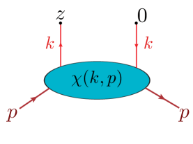
Figure 22: Structure of generic matrix element.

The function $\chi(k,p)$ depends on the momenta $k$ and $p$. The analysis of Feynman diagrams in the Schwinger $\alpha$-representation (see, e.g., Ref. [76]) tells that, a general scalar handbag diagram $d_{i}$ of the Fig. 22 type may be written as

$$i\chi_{d_{i}}(k,p)=i^{l}\,\frac{P({\rm c.c.})}{(4\pi i)^{2L}}\int_{0}^{\infty}\prod_{j=1}^{l}d\alpha_{j}[D(\alpha)]^{-2}$$

$$\times\exp\left\{ik^{2}\frac{A(\alpha)}{D(\alpha)}+i\frac{(p-k)^{2}B_{s}(\alpha)+(p+k)^{2}B_{u}(\alpha)}{D(\alpha)}\right\}$$

$$\times\exp\left\{ip^{2}\frac{C(\alpha)}{D(\alpha)}-i\sum_{j}\alpha_{j}(m_{j}^{2}-i\epsilon)\right\}\ ,$$ (1.20)

where ${P({\rm c.c.})}$ is the relevant product of coupling constants, $L$ is the number of loops of the diagram, $l$ is the number of its lines, and the argument $(\alpha)$ of the $A,B,C,D$ functions should be understood as $(\{\alpha_{d_{i}}\})$. Using this representation, we get

$$i\chi(k,p)=\int_{0}^{\infty}d\lambda\,\int_{-1}^{1}dx\,e^{i\lambda[k^{2}-2x(kp)+i\epsilon]}\,F(x,\lambda;p^{2})$$ (1.21)

where the function $F(x,\lambda;p^{2})$ is given by the sum over all contributing diagrams,

$$F(x,\lambda;p^{2})=\sum_{d_{i}}\int_{0}^{\infty}d\lambda_{d_{i}}\delta(\lambda-\lambda_{d_{i}})\int_{-1}^{1}\differential x_{d_{i}}\delta(x-x_{d_{i}})\ \,F_{d_{i}}(x_{d_{i}},\lambda_{d_{i}};p^{2})\ ,$$ (1.22)

with the functions $F_{d_{i}}(x_{d_{i}},\lambda_{d_{i}};M^{2})$ specific for each diagram, and

$$\lambda_{d_{i}}= \frac{A_{d_{i}}(\alpha)+{B_{s}}_{\,d_{i}}(\alpha)+{B_{u}}_{\,d_{i}}(\alpha)}{D_{d_{i}}(\alpha)}\ \ ,$$ (1.23)

$$x_{d_{i}}= \frac{{B_{s}}_{\,d_{i}}(\alpha)-{B_{u}}_{\,d_{i}}(\alpha)}{A_{\,d_{i}}(\alpha)+{B_{s}}_{\,d_{i}}(\alpha)+{B_{u}}_{\,d_{i}}(\alpha)}\ .$$ (1.24)

Eq. (1.21) expresses an evident fact that the function $\chi(k,p)$ depends on $k$ through the Lorentz invariants $(kp)$ and $k^{2}$. A nontrivial property is that $A(\alpha)$, $B_{s}(\alpha)$, $B_{u}(\alpha)$, $C(\alpha)$ and $D(\alpha)$ are non-negative functions, namely, sums of products of non-negative $\alpha_{j}$-parameters of a diagram. This immediately gives $0\leq\lambda\leq\infty$. The limits for $x$ in general case are obviously $-1\leq x\leq 1$. The negative $x$ values appear when $B_{u}(\alpha)\neq 0$, which happens for some nonplanar diagrams. Integrating over $\lambda$ in Eq. (1.21) gives a Nakanishi-type representation[77] for this amplitude.

Note that no restrictions are imposed on $k$ and $p$ in Eq. (1.21). In particular, $p$ is the actual external momentum with $p^{2}=M^{2}$. Transforming Eq. (1.21) to the coordinate representation and changing $\lambda=1/\sigma$ gives

$$\langle p|\phi(0)\phi(z)|p\rangle= \int_{0}^{\infty}d\sigma\int_{-1}^{1}\differential x\,\Phi(x,\sigma;M^{2})\,\,e^{-ix(pz)-i\sigma{(z^{2}-i\epsilon)}/{4}}\,\$$ (1.25)

where

$$\Phi(x,\sigma;M^{2})=\exp[-ix^{2}M^{2}/\sigma]F(x,1/\sigma;M^{2})$$ (1.26)

is the Virtuality Distribution Function[78, 79] (VDF) and Eq. (1.25) is the VDF representation. It basically reflects the fact that the matrix element $\langle p|\phi(0)\phi(z)|p\rangle$ depends on $z$ through $(pz)$ and $z^{2}$.

The main non-trivial feature of the representations (1.21), (1.25) is in their specific limits of integration over $x$ and $\lambda$ (or $\sigma$). These are dictated by the properties of the contributing Feynman diagrams, in particular, by positivity of the functions $A,B,D$ determining $x$ and $\lambda$. It should be emphasized that these functions are determined purely by denominators of propagators, and are not affected by their numerators present in non-scalar theories.

Thus, the VDF representation (1.25) is valid for any diagram and reflects very general features of quantum field theory. On these grounds, we assume that it holds nonperturbatively. Integrating over $\sigma$, we get the pseudo-PDF representation

$$\langle p|\phi(0)\phi(z)|p\rangle= \int_{-1}^{1}\differential x\,{\cal P}(x,-z^{2})\,\,e^{-ix(pz)}\,\ .$$ (1.27)

Eq. (1.27) gives a covariant definition of $x$ as a variable that is Fourier-conjugate to the Ioffe time $(pz)$. To define $x$, we do not need to assume that $p^{2}=0$ or that $z^{2}=0$. We also do not need to base the definition of $x$ on the ideas of the light-front quantization, the analysis in the infinite momentum frame, Sudakov variables, etc.

References

- [1] R. P. Feynman, “Photon-hadron interactions”, Reading, 282p (1972)
- [2] W. Detmold and C. J. D. Lin, Phys. Rev. D 73, 014501 (2006)
- [3] V. Braun and D. Müller, Eur. Phys. J. C 55, 349 (2008)
- [4] X. Ji, Phys. Rev. Lett. 110, 262002 (2013)
- [5] K. Cichy and M. Constantinou, Adv. High Energy Phys. 2019, 3036904 (2019)
- [6] A. V. Radyushkin, JINR preprint P2-10717 (1977); [hep-ph/0410276].
- [7] D. Müller, D. Robaschik, B. Geyer, F.-M. Dittes and J. Hořejši, Fortsch. Phys. 42, 101 (1994)
- [8] X. D. Ji, Phys. Rev. Lett. 78, 610 (1997)
- [9] A. V. Radyushkin, Phys. Rev. D 56, 5524 (1997)
- [10] B. L. Ioffe, Phys. Lett. 30B, 123 (1969)
- [11] A. V. Radyushkin, Phys. Rev. D 96, no. 3, 034025 (2017)
- [12] V. Braun, P. Gornicki and L. Mankiewicz, Phys. Rev. D 51, 6036 (1995)
- [13] A. V. Radyushkin, Phys. Lett. 131B, 179 (1983)
- [14] A. Radyushkin, Phys. Lett. B 767, 314 (2017)
- [15] X. Ji, Sci. China Phys. Mech. Astron. 57, 1407 (2014)
- [16] Y. Zhao, Int. J. Mod. Phys. A 33, no. 36, 1830033 (2019)
- [17] K. Orginos, A. Radyushkin, J. Karpie and S. Zafeiropoulos, Phys. Rev. D 96, no. 9, 094503 (2017)
- [18] Y. Q. Ma and J. W. Qiu, Phys. Rev. D 98, no. 7, 074021 (2018)
- [19] Y. Q. Ma and J. W. Qiu, Phys. Rev. Lett. 120, no. 2, 022003 (2018)
- [20] A. Radyushkin, PoS QCDEV 2017, 021 (2017) [arXiv:1711.06031
- [21] A. V. Radyushkin, Phys. Lett. B 781, 433 (2018)
- [22] A. Radyushkin, Phys. Rev. D 98, no. 1, 014019 (2018)
- [23] J. Karpie, K. Orginos and S. Zafeiropoulos, JHEP 1811, 178 (2018)
- [24] A. V. Radyushkin, Phys. Lett. B 788, 380 (2019)
- [25] A. V. Radyushkin, Phys. Rev. D 100, no. 11, 116011 (2019)
- [26] I. Balitsky, W. Morris and A. Radyushkin, arXiv:1910.13963
- [27] B. Joó, J. Karpie, K. Orginos, A. Radyushkin, D. Richards and S. Zafeiropoulos, JHEP 1912, 081 (2019)
- [28] B. Joó, J. Karpie, K. Orginos, A. V. Radyushkin, D. G. Richards, R. S. Sufian and S. Zafeiropoulos, Phys. Rev. D 100, no. 11, 114512 (2019)
- [29] O. Nachtmann, Nucl. Phys. B 63, 237 (1973)
- [30] H. Georgi and H. D. Politzer, Phys. Rev. D 14, 1829 (1976).
- [31] S. A. Anikin and O. I. Zavyalov, Annals Phys. 116, 135 (1978).
- [32] I. I. Balitsky and V. M. Braun, Nucl. Phys. B 311, 541 (1989)
- [33] A. V. Efremov and A. V. Radyushkin, JINR-E2-11535.
- [34] A. V. Efremov and A. V. Radyushkin, Theor. Math. Phys. 44, 774 (1981) [Teor. Mat. Fiz. 44, 327 (1980)].
- [35] A. V. Efremov and A. V. Radyushkin, Riv. Nuovo Cim. 3N2, 1 (1980)
- [36] V. Fock, Sowjet. Phys. 12, 404 (1937)
- [37] J. S. Schwinger, Phys. Rev. 82, 664 (1951)
- [38] A. M. Polyakov, Nucl. Phys. B 164, 171 (1980)
- [39] V. S. Dotsenko and S. N. Vergeles, Nucl. Phys. B 169, 527 (1980)
- [40] R. A. Brandt, F. Neri and M. a. Sato, Phys. Rev. D 24, 879 (1981)
- [41] S. Aoyama, Nucl. Phys. B 194, 513 (1982)
- [42] N. S. Craigie and H. Dorn, Nucl. Phys. B 185, 204 (1981)
- [43] H. Dorn, Fortsch. Phys. 34, 11 (1986)
- [44] E. Bagan and P. Gosdzinsky, Phys. Lett. B 320, 123 (1994)
- [45] T. Ishikawa, Y. Q. Ma, J. W. Qiu and S. Yoshida, Phys. Rev. D 96, no. 9, 094019 (2017)
- [46] X. Ji, J. H. Zhang and Y. Zhao, Phys. Rev. Lett. 120, no. 11, 112001 (2018)
- [47] J. Green, K. Jansen and F. Steffens, Phys. Rev. Lett. 121, no. 2, 022004 (2018)
- [48] V. M. Braun, A. Vladimirov and J. H. Zhang, Phys. Rev. D 99, no. 1, 014013 (2019)
- [49] A. V. Radyushkin, Fiz. Elem. Chast. Atom. Yadra 14, 58 (1983)
- [50] M. Anselmino, M. Boglione, J. O. Gonzalez Hernandez, S. Melis and A. Prokudin, JHEP 1404, 005 (2014)
- [51] B. U. Musch, P. Hagler, J. W. Negele and A. Schafer, Phys. Rev. D 83, 094507 (2011)
- [52] H. W. Lin, J. W. Chen, S. D. Cohen and X. Ji, Phys. Rev. D 91, 054510 (2015)
- [53] C. Alexandrou, K. Cichy, M. Constantinou, K. Hadjiyiannakou, K. Jansen, F. Steffens and C. Wiese, Phys. Rev. D 96, no. 1, 014513 (2017)
- [54] C. Alexandrou, K. Cichy, M. Constantinou, K. Hadjiyiannakou, K. Jansen, A. Scapellato and F. Steffens, Phys. Rev. D 99, no. 11, 114504 (2019)
- [55] R. Barbieri, J. R. Ellis, M. K. Gaillard and G. G. Ross, Nucl. Phys. B 117, 50 (1976)
- [56] R. K. Ellis, W. Furmanski and R. Petronzio, Nucl. Phys. B 212, 29 (1983)
- [57] A. Radyushkin, Phys. Lett. B 770, 514 (2017)
- [58] J. W. Chen, S. D. Cohen, X. Ji, H. W. Lin and J. H. Zhang, Nucl. Phys. B 911, 246 (2016)
- [59] G. Altarelli and G. Parisi, Nucl. Phys. B 126, 298 (1977)
- [60] V. N. Gribov and L. N. Lipatov, Sov. J. Nucl. Phys. 15, 438 (1972) [Yad. Fiz. 15, 781 (1972)].
- [61] Y. L. Dokshitzer, Sov. Phys. JETP 46, 641 (1977) [Zh. Eksp. Teor. Fiz. 73, 1216 (1977)].
- [62] J. W. Chen, X. Ji and J. H. Zhang, Nucl. Phys. B 915, 1 (2017)
- [63] T. Izubuchi, X. Ji, L. Jin, I. W. Stewart and Y. Zhao, Phys. Rev. D 98, no. 5, 056004 (2018)
- [64] X. Ji, J. H. Zhang and Y. Zhao, Nucl. Phys. B 924, 366 (2017)
- [65] J. H. Zhang, J. W. Chen and C. Monahan, Phys. Rev. D 97, no. 7, 074508 (2018)
- [66] J. Karpie, K. Orginos, A. Rothkopf and S. Zafeiropoulos, JHEP 1904, 057 (2019)
- [67] A. Accardi, L. T. Brady, W. Melnitchouk, J. F. Owens and N. Sato, Phys. Rev. D 93, no. 11, 114017 (2016)
- [68] K. Cichy, L. Del Debbio and T. Giani, JHEP 1910, 137 (2019)
- [69] L. A. Harland-Lang, A. D. Martin, P. Motylinski and R. S. Thorne, Eur. Phys. J. C 75, no. 5, 204 (2015)
- [70] A. D. Martin, W. J. Stirling, R. S. Thorne and G. Watt, Eur. Phys. J. C 63, 189 (2009)
- [71] R. D. Ball et al. [NNPDF Collaboration], Eur. Phys. J. C 77, no. 10, 663 (2017)
- [72] G. P. Lepage and S. J. Brodsky, Phys. Rev. D 22, 2157 (1980)
- [73] A. V. Radyushkin, Phys. Rev. D 95, no. 5, 056020 (2017)
- [74] A. V. Radyushkin, Phys. Rev. D 59, 014030 (1999)
- [75] E. E. Salpeter and H. A. Bethe, Phys. Rev. 84, 1232 (1951)
- [76] N. Nakanishi, Graph Theory and Feynman Integrals, Gordon and Breach, New York, (1971)
- [77] N. Nakanishi, Prog. Theor. Phys. Suppl. 43, 1 (1969)
- [78] A. V. Radyushkin, Phys. Lett. B 735, 417 (2014)
- [79] A. V. Radyushkin, Phys. Rev. D 93, no. 5, 056002 (2016)