Alternating conditional gradient method for
convex feasibility problems

Abstract

The classical convex feasibility problem in a finite dimensional Euclidean space is studied in the present paper. We are interested in two cases. First, we assume to know how to compute an exact project onto one of the sets involved and the other set is compact such that the conditional gradient (CondG) method can be used for computing efficiently an inexact projection on it. Second, we assume that both sets involved are compact such that the CondG method can be used for computing efficiently inexact projections on them. We combine alternating projection method with CondG method to design a new method, which can be seen as an inexact feasible version of alternate projection method. The proposed method generates two different sequences belonging to each involved set, which converge to a point in the intersection of them whenever it is not empty. If the intersection is empty, then the sequences converge to points in the respective sets whose distance is equal to the distance between the sets in consideration.

Keywords: Convex feasibility problem, alternating projection method, conditional gradient method, inexact projections.

AMS: 65K05, 90C30, 90C25.

1 Introduction

The classic convex feasibility problem consists of finding a point in the intersection of two sets. It is formally state as follows:

$$\mbox{find }x_{*}\in A\cap B,$$ (1)

where $A,B\subset\mathbb{R}^{n}$ are convex, closed, and nonempty sets. Although we are not concerned with practical issues at this time, we emphasize that several practical applications appear modeled as Problem (1); see for example [14, 15, 27] and references therein. Among the methods to solve Problem (1), the alternating projection method is one of the most interesting and popular, with a long history dating back to J. von Neumann [34]. Since this seminal work, the alternating projection method has attracted the attention of the scientific community working on optimization, papers dealing with this method include [1, 8, 11]. Perhaps one of the factors that explains this interest is its simplicity and ease of implementation, making application to large-scale problems very attractive. Several variants of this method have arisen and several theoretical and practical issues related to it have been discovered over the years, resulting in a wide literature on the subject. For a historical perspective of this method; see, for exemple [3] and a complete annotated bibliography of books and review can be found in [10].

The aim of this paper is present a new method to solve Problem 1. The proposed method is based on the alternating projection method. For design the method, the conditional gradient method (CondG method) also known as Frank-Wolfe algorithm developed by Frank and Wolfe in 1956 [20] (see also [31]) is used to compute feasible inexact projections on the sets in consideration, which will be named as alternating conditional gradient (ACondG) method. We present two versions of the method. First, we assume that we know how to compute an exact project onto one of the sets involved. Besides, we assume that the other set is compact with a special structure such that CondG method can be used for computing efficiently feasible inexact projections on it. Second, we assume that both sets are compact with special structures such that the CondG method can be used for computing feasible inexact projections on them. The ACondG method proposed, generates two sequences $(x^{k})_{k\in\mathbb{N}}\subset A$ and $(y^{k})_{k\in\mathbb{N}}\subset B$. The mains obtained results are as follows. If $A\cap B\neq\varnothing$, then the sequences $(x^{k})_{k\in\mathbb{N}}$ and $(y^{k})_{k\in\mathbb{N}}$ converge to a point $x^{*}$ belonging to $A\cap B$. If $A\cap B=\varnothing$, then the sequences $(x^{k})_{k\in\mathbb{N}}$ and $(y^{k})_{k\in\mathbb{N}}$, converge respectively to $x^{*}\in A$ and $y^{*}\in B$ satisfying $\|x^{*}-y^{*}\|=dist(A,B)$, where $dist(A,B)$ denotes the distance between the sets $A$ and $B$.

From a practical point of view, considering methods that use inexact projections are particularly interesting. Indeed, one drawback of methods that use exact projections is the need to solve a quadratic problem at each stage, which may substantially increasing the cost per iteration if the number of unknowns is large. In fact, it may not be justified to carry out exact projections when the iterates are far from the solution of the problem. For this reason, seeking to make the alternating projection method more efficient, we use the CondG method to compute feasible inexact projections rather than exact ones. It is noteworthy that the CondG method is easy to implement, has low computational cost per iteration, and readily exploits separability and sparsity, resulting in high computational performance in different classes of compact sets, see [19, 21, 24, 29, 31]. Therefore, we believe that all of these features accredit the method as being quite appropriate for our purpose, which has also been used for similar aims [12, 22, 25, 33]. As aforementioned, the proposed method performs iterations alternately on the sets $A$ and $B$ only approximately, but them become increasingly accurate in relation to the progress of previous iterations. Therefore, the resulting method can be seen as an inexact version of the classical alternate projection method. It is worth noting that others approximate projections have been widely used in the literature. For instance, approximate projection can be performed by projecting onto the hyperplane separating the set and the point to be projected, see [23], and for more examples, see [4, 9, 16, 17, 18, 28]. However, inexact projections obtained in this way are infeasible to the set to be projected, in contrast with feasible inexact projections propose here. Moreover, as far as we know, the combination of the conditional method with the alternate directions method for designing a new method to solve Problem (1) has not yet been considered.

The organization of the paper is as follows. In section 2, we present some notation and basic results used in our presentation. In section 3 we describe the conditional gradient method and present some results related to it. In sections 4 and we present, respectively, the first and second version of inexact alternating projection method to solve Problem (1). Some numerical experiments are provided in section 6. We conclude the paper with some remarks in section 7.

Notation. We denote: ${\mathbb{N}}=\{0,1,2,\ldots\}$, $\langle\cdot,\cdot\rangle$ is the usual inner product, $\|\cdot\|$ is the Euclidean norm, and $[v]_{i}$ is the $i$-th component of the vector $v$.

2 Preliminaries

In this section, we present some preliminary results used throughout the paper. The projection onto a closed convex set $C\subset\mathbb{R}^{n}$ is the mapping $P_{C}:\mathbb{R}^{n}\to C$ defined by

$$P_{C}(v):=\arg\min_{z\in C}\|v-z\|.$$

In the next lemma we present some important properties of the projection mapping.

Lemma 1.

Let $C\subset\mathbb{R}^{n}$ be any nonempty closed and convex set and $P_{C}$ the projection mapping onto $C$. For all $v\in\mathbb{R}^{n}$, the following properties hold:

1. $\langle v-P_{C}(v),z-P_{C}(v)\rangle\leq 0$, for all $z\in C$;

2. $\|{P}_{C}(v)-z\|^{2}\leq\|v-z\|^{2}-\|{P}_{C}(v)-v\|^{2}$, for all $z\in C$;

3. the projection mapping $P_{C}$ is continuous.

Proof.

The items (i) and (iii) are proved in [5, Proposition 3.10, Theorem 3.14]. For item (ii), combine $\|v-z\|^{2}=\|{P}_{C}(v)-v\|^{2}+\|{P}_{C}(v)-z\|^{2}-2\langle{P}_{C}(v)-v,{P}_{C}(v)-z\rangle$ with item (i). ∎

Let $C,D\subset\mathbb{R}^{n}$ be convex, closed, and nonempty sets. Define the distance between the sets $C$ and $D$ by $dist(C,D):=\inf\{\|v-w\|:~{}v\in C,w\in D\}$.

Lemma 2.

Let $C$ be a compact and convex set and $D$ be a closed and convex set. Assume that the sequences $(v^{k})_{k\in\mathbb{N}}\subset C$ and $(w^{k})_{k\in\mathbb{N}}\subset D$ satisfy the following two conditions:

• $\lim_{k\to+\infty}\|v^{k+1}-v^{k}\|=0$ and $\lim_{k\to+\infty}\|w^{k+1}-w^{k}\|=0$;

• $\lim_{k\to+\infty}\|w^{k+1}-P_{D}(v^{k})\|=0$ and $\lim_{k\to+\infty}\|v^{k+1}-P_{C}(w^{k+1})\|=0$.

Then, each cluster point ${\bar{v}}$ of $(v^{k})_{k\in\mathbb{N}}$ is a fixed point of $P_{C}P_{D}$, i.e., ${\bar{v}}=P_{C}P_{D}({\bar{v}})$. Moreover, $\lim_{k\to\infty}\|v^{k}-w^{k}\|=dist(C,D)$ and $\lim_{k\to\infty}(v^{k}-w^{k})=P_{C-D}(0)$, where $P_{C-D}(0):=\arg\min_{v\in C,w\in D}\|v-w\|$.

Proof.

Let ${\bar{v}}$ be a cluster point of $(v^{k})_{k\in\mathbb{N}}$. Let $(v^{k_{j}})_{j\in\mathbb{N}}$ be a subsequence of $(v^{k})_{k\in\mathbb{N}}$ with $\lim_{{j}\to+\infty}v^{k_{j}}={\bar{v}}$ and consider $(w^{k_{j}+1})_{j\in\mathbb{N}}$ which is a subsequence of $(w^{k+1})_{k\in\mathbb{N}}$. Since $C$ is compact, $(v^{k})_{k\in\mathbb{N}}\subset C$ and $\lim_{k\to+\infty}\|w^{k+1}-P_{D}(v^{k})\|=0$, we conclude that $(w^{k_{j}+1})_{j\in\mathbb{N}}$ is bounded. Thus, there exists a cluster point ${\bar{w}}$ of $(w^{k_{j}+1})_{j\in\mathbb{N}}$ and a subsequence $(w^{k_{\ell}+1})_{\ell\in\mathbb{N}}$ of $(w^{k_{j}+1})_{j\in\mathbb{N}}$ with $\lim_{{\ell}\to+\infty}w^{k_{\ell}+1}={\bar{w}}$. Futhermore, the corresponding subsequence $(v^{k_{\ell}})_{j\in\mathbb{N}}$ of $(v^{k_{j}})_{j\in\mathbb{N}}$ also satisfies $\lim_{{\ell}\to+\infty}v^{k_{\ell}}={\bar{v}}$. Due to $(\|v^{k+1}-v^{k}\|^{2})_{k\in\mathbb{N}}$ and $(\|w^{k+1}-w^{k}\|^{2})_{k\in\mathbb{N}}$ converge to zero, we also have $\lim_{{\ell}\to+\infty}v^{k_{\ell}+1}={\bar{v}}$ and $\lim_{{\ell}\to+\infty}w^{k_{\ell}}={\bar{w}}$. Moreover, it follows from Lemma 1 (ii) and conditions (c1) and (c2) that

$${\bar{w}}=P_{D}({\bar{v}}),\qquad{\bar{v}}=P_{C}({\bar{w}}),$$

respectively. Hence, last equalities imply ${\bar{v}}=P_{C}P_{D}({\bar{v}})$ and, by using [11, Theorem 2], we have $\|{\bar{v}}-P_{D}({\bar{v}})\|=dist(C,D)$. Therefore, we conclude that each cluster point ${\bar{v}}$ of $(v^{k})_{k\in\mathbb{N}}$ is a fixed point of $P_{C}P_{D}$, i.e., ${\bar{v}}=P_{C}P_{D}({\bar{v}})$, which proves the first statement. Moreover, for each subsequence $(v^{k_{\ell}})_{\ell\in\mathbb{N}}$ of $(v^{k})_{k\in\mathbb{N}}$ such that $\lim_{{\ell}\to+\infty}v^{k_{\ell}}={\bar{v}}$, there exists a subsequence $(w^{k_{\ell}})_{\ell\in\mathbb{N}}$ of $(w^{k})_{k\in\mathbb{N}}$ with $\lim_{{\ell}\to+\infty}w^{k_{\ell}}=P_{D}({\bar{v}})$ and $\|{\bar{v}}-P_{D}({\bar{v}})\|=dist(C,D)$. Consequently, the sequence $(\|v^{k}-w^{k}\|)_{k\in\mathbb{N}}$ converges to the distance between $A$ and $B$, i.e., $\lim_{k\to\infty}\|v^{k}-w^{k}\|=dist(C,D)$ and this proves the second statement. Considering that $D$ is a closed convex set and $C$ is a compact convex set, it follows that $C-D$ is also a closed and convex set, which implies $P_{C-D}(0)$ is a singleton. Therefore, we obtain that $(v^{k}-w^{k})_{k\in\mathbb{N}}$ converges to $P_{A-B}(0)$, i.e., $\lim_{k\to\infty}(v^{k}-w^{k})=P_{C-D}(0)$ (see, [2, Lemma 2.3]), concluding the proof of the lemma. ∎

Definition 1.

Let $S$ be a nonempty subset of $\mathbb{R}^{n}$. A sequence $(v^{k})_{k\in\mathbb{N}}\subset\mathbb{R}^{n}$ is said to be quasi-Fejér convergent to $S$, if and only if, for all $v\in S$ there exists $k_{0}\geq 0$ and a summable sequence $(\epsilon_{k})_{k\in\mathbb{N}}$, such that $\|v^{k+1}-v\|^{2}\leq\|v^{k}-v\|^{2}+\epsilon_{k}$ for all $k\geq k_{0}$. If for all $k\in\mathbb{N}$, $\epsilon_{k}=0$, the sequence $(v^{k})_{k\in\mathbb{N}}$ is said to be Fejér convergent to $S$.

Lemma 3.

Let $(v^{k})_{k\in\mathbb{N}}$ be quasi-Fejér convergent to $S$. Then, the following conditions hold:

• the sequence $(v^{k})_{k\in\mathbb{N}}$ is bounded;

• for all $v\in S$, the sequence $(\|v^{k}-v\|)_{k\in\mathbb{N}}$ is convergent.

• if a cluster point ${\bar{v}}$ of $(v^{k})_{k\in\mathbb{N}}$ belongs to $S$, then $(v^{k})_{k\in\mathbb{N}}$ converges to ${\bar{v}}$.

3 Conditional gradient (CondG) method

In the following we remind the classical conditional gradient method (CondG_C) to compute feasible inexact projections with respect to a compact convex set $C$ and some results related to it. We also prove two important inequalities related to this method that will be useful to establish our main results. For presenting the method, we assume the existence of a linear optimization oracle (or simply LO oracle) capable of minimizing linear functions over the constraint set $C$. We formally state the CondG_C method to calculate an inexact projection of $v\in{\mathbb{R}}^{n}$ with respect $u\in C$, with the following input data: a relative error tolerance function $\varphi:{\mathbb{R}}^{n}\times{\mathbb{R}}^{n}\times{\mathbb{R}}^{n}\to{\mathbb{R}}_{+}$ satisfying the following inequality

$$\varphi_{\gamma,\theta,\lambda}(u,v,w)\leq\gamma\|v-u\|^{2}+\theta\|w-v\|^{2}+\lambda\|w-u\|^{2},\qquad\forall~{}u,v,w\in{\mathbb{R}}^{n},$$ (2)

where $\gamma,\theta,\lambda\geq 0$ are given forcing parameters.

Input:

Take $\gamma,\theta,\lambda\in{\mathbb{R}}_{+}$, $v\in{\mathbb{R}}^{n}$, $u,w\in C$, and $\varphi_{\gamma,\theta,\lambda}$. Set $w_{0}=w$ and $\ell=0$.

Step 1.

Use a LO oracle to compute an optimal solution $z_{\ell}$ and the optimal value $s_{\ell}^{*}$ as

$$z_{\ell}:=\arg\min_{z\in C}\,\langle w_{\ell}-v,~{}z-w_{\ell}\rangle,\qquad s_{\ell}^{*}:=\langle w_{\ell}-v,~{}z_{\ell}-w_{\ell}\rangle.$$ (3)

Step 2.

If $-s^{*}_{\ell}\leq\varphi_{\gamma,\theta,\lambda}(u,v,w_{\ell})$, then stop. Set $w^{+}:=w_{\ell}$.

Step 3.

Compute $\alpha_{\ell}\in\,(0,1]$ and $w_{\ell+1}$ as

$$w_{\ell+1}:=w_{\ell}+\alpha_{\ell}(z_{\ell}-w_{\ell}),\qquad{\alpha}_{\ell}:=\min\left\{1,\frac{-s^{*}_{\ell}}{\|z_{\ell}-w_{\ell}\|^{2}}\right\}.$$ (4)

Step 4.

Set $\ell\leftarrow\ell+1$, and go to step 1.

Output:

$w^{+}:=w_{\ell}$.

Algorithm 1 CondG_C method $w^{+}$:=CondG_C $(\varphi_{\gamma,\theta,\lambda},u,v)$

Let us describe the main features of CondG_C method; for further details, see, for example, [6, 29, 30]. Let $v\in{\mathbb{R}}^{n}$, $\psi:\mathbb{R}^{n}\to\mathbb{R}$ be defined by $\psi(z):=\|z-v\|^{2}/2$, and $C\subset{\mathbb{R}}^{n}$ a convex compact set. It is worth mentioning that the above CondG_C method can be viewed as a specialized version of the classic conditional gradient method applied to the problem $\min_{z\in C}\psi(z)$. In this case, (3) is equivalent to $s_{\ell}^{*}:=\min_{z\in C}\langle\psi^{\prime}(w_{\ell}),~{}z-w_{\ell}\rangle$. Since $\psi$ is convex we have

$$\psi(z)\geq\psi(w_{\ell})+\langle\psi^{\prime}(w_{\ell}),~{}z-w_{\ell}\rangle\geq\psi(w_{\ell})+s_{\ell}^{*},\qquad\forall~{}z\in C.$$

Set $w_{*}:=\arg\min_{z\in C}\psi(z)$ and $\psi^{*}:=\min_{z\in C}\psi(z)$. Letting $z=x_{*}$ in the last inequality we obtain that $\psi(w_{\ell})\geq\psi^{*}\geq\psi(w_{\ell})+s_{\ell}^{*}$, which implies that $s_{\ell}^{*}\leq 0$. Thus, we conclude that

$$-s_{\ell}^{*}=\langle v-w_{\ell},~{}z_{\ell}-w_{\ell}\rangle\geq 0\geq\langle v-w_{*},~{}z-w_{*}\rangle,\qquad\forall~{}z\in C.$$

Therefore, we state the stopping criteria as $-s_{\ell}^{*}\leq\varphi_{\gamma,\theta,\lambda}(u,v,w_{\ell})$. Moreover, if the CondG_C method computes $w_{\ell}\in C$ satisfying $-s_{\ell}^{*}\leq\varphi_{\gamma,\theta,\lambda}(u,v,w_{\ell})$, then the method terminates. Otherwise, it computes the stepsize $\alpha_{\ell}=\arg\min_{\alpha\in[0,1]}\psi(w_{\ell}+\alpha(z_{\ell}-w_{\ell}))$ using exact minimization. Since $z_{\ell}$, $w_{\ell}\in C$ and $C$ is convex, we conclude from (4) that $w_{\ell+1}\in C$, thus the CondG_C method generates a sequence in $C$. Finally, (3) implies that $\langle v-w_{\ell},~{}z-w_{\ell}\rangle\leq-s_{\ell}^{*}$, for all $z\in C$. Hence, considering the stopping criteria $-s_{\ell}^{*}\leq\varphi_{\gamma,\theta,\lambda}(u,v,w_{\ell})$, we conclude that the output of CondG_C method is a feasible inexact projection $w^{+}=\mbox{CondG${}_{C}$}\,(\varphi_{\gamma,\theta,\lambda},u,v)$ of the point $v\in{\mathbb{R}}^{n}$ with respect $u\in C$ onto $C$, i.e.,

$$\langle v-w^{+},~{}z-w^{+}\rangle\leq\varphi_{\gamma,\theta,\lambda}(u,v,w^{+}),\qquad\forall~{}z\in C.$$ (5)

Remark 1.

Since $C\subset{\mathbb{R}}^{n}$ is a closed convex set, then by Lemma 1 (i) together with (5) we obtain, for any $v\in{\mathbb{R}}^{n}$ and $u\in C$, that ${P}_{C}(v)=\mbox{CondG${}_{C}$}\,(\varphi_{0,0,0},u,v)$, where ${P}_{C}(v)$ denotes the exact projection of $v$ onto $C$ and $\varphi_{0,0,0}(u,v,w)\equiv 0$.

The following two theorem state well-known convergence rate for classic conditional gradient method applied to problem $\min_{z\in C}\psi(z)$, see [24, 29, 31]. Let us first remind some basic properties of the function $\psi$ over the set $C$:

• $\psi(z)=\psi(w)+\langle\psi^{\prime}(w),~{}z-w\rangle+\|z-w\|^{2}/2$, for all $z,w\in C$;

• $\psi(z)-\psi(w_{*})\geq\|z-w_{*}\|^{2}/2$, for all $z\in C$;

• $\|\psi^{\prime}(z)\|\geq\psi(w_{*})=d(v,C)$, for all $z\in C$.

Since $C$ is a compact set, we define the diameter of $C$ by $d_{C}:=\max_{z,w\in C}\|z-w\|$. The statement of the first convergence result is as follows.

Theorem 4.

Let $\{w_{\ell}\}$ be the sequence generated by Algorithm 1. Then, $\psi(w_{\ell})-\psi(w_{*})\leq(8d_{C}^{2})/\ell$, for all $\ell\geq 1$. Consequently, (by using item (ii) above) we have $\|w_{\ell}-w_{*}\|\leq 4d_{C}/\ell$, for all $\ell\geq 1$.

The rate of convergence in Theorem 4 is improved for $\alpha_{C}$-strongly convex. We say that a convex set $C$ is $\alpha_{C}$-strongly convex if, for any $z,w\in C$, $t\in[0,1]$ and any vector $u\in{\mathbb{R}}^{n}$, it holds that $tz+(1-t)w+(\alpha_{C}/2)t(1-t)\|z-w\|^{2}u\in C$.

Theorem 5.

Assume that $C$ is a $\alpha_{C}$-strongly convex set. Let $\{w_{\ell}\}$ be the sequence generated by Algorithm 1 and set $q:=\max\{1/2,1-\alpha_{C}d(v,C)/8\}<1$. Then, $\psi(w_{\ell+1})-\psi(w_{*})\leq q\left(\psi(w_{\ell})-\psi(w_{*})\right)$, for all $\ell\geq 1$. Consequently, we have an exponentially convergence rate as follows $\psi(w_{\ell})-\psi(w_{*})\leq(\psi(w_{0})-\psi(w_{*}))q^{\ell}$, for all $\ell\geq 1$. Furthermore, (by using item (ii) above) we have $\|w_{\ell}-w_{*}\|\leq(\psi(w_{0})-\psi(w_{*}))q^{\ell}$, for all $\ell\geq 1$.

Let us present two useful properties of CondG_C method that will play important roles in the remainder of this paper.

Lemma 6.

Let $v\in{\mathbb{R}}^{n}$, $u\in C$, $\gamma,\theta,\lambda\geq 0$ and $w^{+}=\mbox{CondG${}_{C}$}\,(\varphi_{\gamma,\theta,\lambda},u,v)$. Then, there holds

$$\|w^{+}-z\|^{2}\leq\|v-z\|^{2}+\frac{2\gamma+2\lambda}{1-2\lambda}\|v-u\|^{2}-\frac{1-2\theta}{1-2\lambda}\|w^{+}-v\|^{2},\qquad z\in C,$$ (6)

for $0\leq\lambda<1/2$. Consequently, if $z=P_{C}(v)$ then

$$\|w^{+}-P_{C}(v)\|^{2}\leq\frac{2\gamma+2\lambda}{1-2\lambda}\|v-u\|^{2}+\frac{2\theta}{1-2\lambda}\|w^{+}-v\|^{2}.$$ (7)

Proof.

First, note that $\|w^{+}-z\|^{2}=\|v-z\|^{2}-\|v-w^{+}\|^{2}+2\langle v-w^{+},z-w^{+}\rangle$, for all $z\in C$. Since $w^{+}=\mbox{CondG${}_{C}$}\,(\varphi_{\gamma,\theta,\lambda},u,v)$, combining the last inequality with (5) and (2), after some algebraic manipulation, we obtain

$$\|w^{+}-z\|^{2}\leq\|v-z\|^{2}+2\gamma\|v-u\|^{2}-(1-2\theta)\|v-w^{+}\|^{2}+2\lambda\|w^{+}-u\|^{2},\qquad z\in C.$$ (8)

On the other hand, $\|w^{+}-u\|^{2}=\|w^{+}-v\|^{2}+\|u-v\|^{2}-2\langle w^{+}-v,u-v\rangle$, which implies that

$$\|w^{+}-u\|^{2}=\|u-v\|^{2}-\|w^{+}-v\|^{2}+2\langle v-w^{+},u-w^{+}\rangle.$$

Since $w^{+}=\mbox{CondG${}_{C}$}\,(\varphi_{\gamma,\theta,\lambda},u,v)$ and $u\in C$, using (5) with $z=u$ and (2) with $w=w^{+}$, after some calculations, the last equation implies

$$\|w^{+}-u\|^{2}\leq\frac{1+2\gamma}{1-2\lambda}\|v-u\|^{2}-\frac{1-2\theta}{1-2\lambda}\|w^{+}-v\|^{2}.$$

Combining last inequality with (8) we obtain (6). We proceed to prove (7). First note that letting $z=P_{B}(v)$ into inequality (6), the resulting inequality can be equivalently rewriting as follows

$$\|w^{+}-P_{C}(v)\|^{2}\leq\|v-P_{C}(v)\|^{2}-\|w^{+}-v\|^{2}+\frac{2\gamma+2\lambda}{1-2\lambda}\|v-u\|^{2}-\frac{2\lambda-2\theta}{1-2\lambda}\|w^{+}-v\|^{2}.$$

Thus, considering that $\|v-P_{C}(v)\|^{2}-\|w^{+}-v\|^{2}\leq 0$ and $0\leq\lambda<1/2$ the desired inequality follows, which concludes the proof. ∎

Corollary 7.

Assume that set $E:=\{z\in C:\|z-P_{D}(z)\|=dist(C,D)\}\neq\varnothing$. Let $v\in D$, $u\in C$, $\gamma,\theta,\lambda\geq 0$, $w^{+}=\mbox{CondG${}_{C}$}\,(\varphi_{\gamma,\theta,\lambda},u,v)$. Then, for each ${\bar{z}}\in E$, there holds

$$\|w^{+}-{\bar{z}}\|^{2}\leq\|u-{\bar{z}}\|^{2}+2\langle u-v,P_{D}(\bar{z})-v\rangle+\frac{2\gamma+2\theta}{1-2\lambda}\|v-u\|^{2}-\frac{2\lambda-2\theta}{1-2\lambda}\|w^{+}-v\|^{2}.$$

for $0\leq\lambda<1/2$.

Proof.

Applying (6) of Lemma 6 with $z={\bar{z}}$ we obtain

$$\|w^{+}-{\bar{z}}\|^{2}\leq\|v-{\bar{z}}\|^{2}+\frac{2\gamma+2\lambda}{1-2\lambda}\|v-u\|^{2}-\frac{1-2\theta}{1-2\lambda}\|w^{+}-v\|^{2},$$

which is equivalently to

$$\|w^{+}-{\bar{z}}\|^{2}\leq\|v-{\bar{z}}\|^{2}-\|w^{+}-v\|^{2}+\frac{2\gamma+2\theta}{1-2\lambda}\|v-u\|^{2}-\frac{2\lambda-2\theta}{1-2\lambda}\|w^{+}-v\|^{2}.$$ (9)

First, note that $\|u-v\|^{2}+\|v-{\bar{z}}\|^{2}=\|u-{\bar{z}}\|^{2}+2\langle u-v,{\bar{z}}-v\rangle$. It turns out that $\langle u-v,{\bar{z}}-v\rangle=\langle u-v,{\bar{z}}-P_{D}(\bar{z})\rangle+\langle u-v,P_{D}({\bar{z}})-v\rangle$. Hence, from these two equalities, we obtain

$$\|u-v\|^{2}+\|v-{\bar{z}}\|^{2}=\|u-{\bar{z}}\|^{2}+2\langle u-v,{\bar{z}}-P_{D}(\bar{z})\rangle+2\langle u-v,P_{D}({\bar{z}})-v\rangle.$$ (10)

Due to $\bar{z}\in E$, we have $\|\bar{z}-P_{B}(\bar{z})\|=dist(C,D)\leq\|w^{+}-v\|$ and, by Cauchy-Schwartz inequality, $2\langle u-v,\bar{z}-P_{D}(\bar{z})\rangle\leq 2\|u-v\|\|\bar{z}-P_{D}(\bar{z})\|\leq\|u-v\|^{2}+\|\bar{z}-P_{D}(\bar{z})\|^{2}$. These inequalities imply $2\langle u-v,\bar{z}-P_{D}(\bar{z})\rangle\leq\|u-v\|^{2}+\|w^{+}-v\|^{2}$, which combined with (10) yields

$$\|u-v\|^{2}+\|v-{\bar{z}}\|^{2}\leq\|u-{\bar{z}}\|^{2}+\|u-v\|^{2}+\|w^{+}-v\|^{2}+2\langle u-v,P_{D}({\bar{z}})-v\rangle.$$

This inequality is equivalente to $\|v-{\bar{z}}\|^{2}-\|w^{+}-v\|^{2}\leq\|u-{\bar{z}}\|^{2}+2\langle u-v,P_{D}({\bar{z}})-v\rangle$, which together with (9) yields the desired result. ∎

Let us end this section by presenting some examples of functions satisfying (2).

Example 1.

The functions $\varphi_{1},\varphi_{3},\varphi_{3},\varphi_{4},\varphi_{5},:{\mathbb{R}}^{n}\times{\mathbb{R}}^{n}\times{\mathbb{R}}^{n}\to{\mathbb{R}}_{+}$ defined by $\varphi_{1}(u,v,w):=\gamma\|v-u\|^{2}$, $\varphi_{2}(u,v,w):=\theta\|w-v\|^{2}$, $\varphi_{3}(u,v,w):=\gamma\theta\|v-u\|\|w-v\|$ and $\varphi_{5}(u,v,w)=\gamma\|v-u\|^{2}+\theta\|w-v\|^{2}+\lambda\|w-u\|^{2}$ satisfy (2).

4 The ACondG method with inexact projection onto one set

Next we present our first version of inexact alternating projection method to solve Problem (1), by using the CondG method to compute feasible inexact projections with respect to one of the sets in consideration, which will be named as alternating conditional gradient-1 (ACondG-1) method. For that, we assume that to find an exact project onto the convex set $B$, not necessarily compact, is an easy task. We also assume that $A$ is a convex and compact set and the projection onto it can be approximate by using the CondG_A method. In this case, the ACondG-1 method with feasible inexact projections onto one of the sets, for solving the classic feasibility Problem (1), is formally defined as follows:

Step 0.

Let $(\lambda_{k})_{k\in\mathbb{N}}$, $(\gamma_{k})_{k\in\mathbb{N}}$ and $(\theta_{k})_{k\in\mathbb{N}}$ be sequences of nonnegative real numbers and the associated function $\varphi_{k}:=\varphi_{\gamma_{k},\theta_{k},\lambda_{k}}$, as defined in (2). Let $x_{0}\in A$. If $x^{0}\in B$, then stop. Otherwise, initialize $k\leftarrow 0$.

Step 1.

Compute $P_{B}(x^{k})$ and set the next iterate $y^{k+1}$ as follows

$$y^{k+1}:=P_{B}(x^{k}).$$ (11)

If $y_{k+1}\in A$, then stop.

Step 2.

Use Agorithm 1 to compute $\mbox{CondG${}_{A}$}\,(\varphi_{k},x^{k},y^{k+1})$ and set the iterate $x^{k+1}$ as follows

$$x^{k+1}:=\mbox{CondG${}_{A}$}\,(\varphi_{k},x^{k},y^{k+1}).$$ (12)

If $x_{k+1}\in B$, then stop.

Step 3.

Set $k\leftarrow k+1$, and go to Step 1.

Algorithm 2 CondG method with inexact projection onto one set (ACondG-1)

First of all note that $x^{k}\in A$ and $y^{k}\in B$. Thus, if Algorithm 2 stops, it means that a point belonging to $A\cap B$ has been found. Therefore, we assume that $(x^{k})_{k\in\mathbb{N}}$ and $(y^{k})_{k\in\mathbb{N}}$ generated by Algorithm 2 are infinity sequences. In the following we will analyze Algorithm 2 first assuming that $A\cap B$ is nonempty and, then, considering that $A\cap B$ is empty.

4.1 The ACondG-1 method for two sets with nonempty intersection

In this section we assume that $A\cap B\neq\varnothing$. To proceed with the convergence analysis of ACondG-1 method we need to assume that the forcing sequences $(\lambda_{k})_{k\in\mathbb{N}}$, $(\gamma_{k})_{k\in\mathbb{N}}$ and $(\theta_{k})_{k\in\mathbb{N}}$ satisfy

$$\theta_{k}\leq\theta<1/2,\qquad 2\gamma_{k}+4\lambda_{k}<\sigma<1\qquad k=0,1,\ldots,$$ (13)

where ${\theta}$ and $\sigma$ are positive real constants.

Theorem 8.

The sequences $(x^{k})_{k\in\mathbb{N}}$ and $(y^{k})_{k\in\mathbb{N}}$ converge to a point belonging to $A\cap B\neq\varnothing$.

Proof.

Take any ${\bar{x}}\in A\cap B$. From (11) we have $y^{k+1}=P_{B}(x^{k})$. Then, applying Lemma 1 (ii) with $C=B$, $v=x^{k}$, and $z={\bar{x}}$, we conclude

$$\|y^{k+1}-{\bar{x}}\|^{2}\leq\|x^{k}-{\bar{x}}\|^{2}-\|y^{k+1}-x^{k}\|^{2}.$$ (14)

Using (12) and applying (6) of Lemma 6 with $v=y^{k+1}$, $u=x^{k}$, $\gamma=\gamma_{k}$, $\theta=\theta_{k}$, $\lambda=\lambda_{k}$, $\varphi_{k}=\varphi_{\gamma_{k},\theta_{k},\lambda_{k}}$, $w^{+}=x^{k+1}$, $z={\bar{x}}$, and $C=A$, we obtain

$$\|x^{k+1}-{\bar{x}}\|^{2}\leq\|y^{k+1}-{\bar{x}}\|^{2}+\frac{2\gamma_{k}+2\lambda_{k}}{1-2\lambda_{k}}\|x^{k}-y^{k+1}\|^{2}-\frac{1-2\theta_{k}}{1-2\lambda_{k}}\|x^{k+1}-y^{k+1}\|^{2}.$$ (15)

Therefore, the combination of (14) with (15) yields

$$\|x^{k+1}-{\bar{x}}\|^{2}\leq\|x^{k}-{\bar{x}}\|^{2}-\frac{1-2\gamma_{k}-4\lambda_{k}}{1-2\lambda_{k}}\|x^{k}-y^{k+1}\|^{2}-\frac{1-2\theta_{k}}{1-2\lambda_{k}}\|x^{k+1}-y^{k+1}\|^{2}.$$ (16)

Hence, (13) and (16) imply that $(x^{k})_{k\in\mathbb{N}}$ is Féjer convergent to $A\cap B\neq\varnothing$. Thus, by Lemma 3 (i), $(x^{k})_{k\in\mathbb{N}}$ is bounded. Also, using Lemma 3 (ii), we conclude that $(\|x^{k}-{\bar{x}}\|)_{k\in\mathbb{N}}$ converges. Consequently, from (14) we obtain that $(y^{k})_{k\in\mathbb{N}}$ is also bounded. Since $A$ and $B$ are closed sets, $(x^{k})_{k\in\mathbb{N}}\subset A$, and $(y^{k})_{k\in\mathbb{N}}\subset B$, all cluster cluster points of these sequences belong to the sets $A$ and $B$, respectively. Now, using (16) together with (13), we obtain

$$0<(1-\sigma)\|x^{k}-y^{k+1}\|^{2}\leq\|x^{k}-{\bar{x}}\|^{2}-\|x^{k+1}-{\bar{x}}\|^{2}.$$

Since the right hand side of the last inequality converges to zero, $(\|y^{k+1}-x^{k}\|)_{k\in\mathbb{N}}$ also converges to zero. Thus all cluster points of $(x^{k})_{k\in\mathbb{N}}$ are also clusters points of $(y^{k})_{k\in\mathbb{N}}$, proving that there exists ${\hat{x}}\in A\cap B$ a cluster point of $(x^{k})_{k\in\mathbb{N}}$ and $(y^{k})_{k\in\mathbb{N}}$. Therefore, from Lemma 3 (iii) we conclude that $(x^{k})_{k\in\mathbb{N}}$ and $(y^{k})_{k\in\mathbb{N}}$ converge to a same point in $A\cap B$. ∎

4.2 The ACondG-1 method for two sets with empty intersection

In the following we assume that the sets $A$ and $B$ have empty intersection, i.e., $A\cap B=\varnothing$. Since $A$ is a compact set and the projection mapping $P_{B}$ is continuous we have

$$\zeta:=\sup\{\|x-P_{B}(u)\|:~{}x,u\in A\}<+\infty.$$ (17)

Let us also assume in this section that $(\lambda_{k})_{k\in\mathbb{N}}$, $(\gamma_{k})_{k\in\mathbb{N}}$ and $(\theta_{k})_{k\in\mathbb{N}}$ are summable,

$$\sum_{k\in\mathbb{N}}\gamma_{k}<\infty,\qquad\quad\sum_{k\in\mathbb{N}}\theta_{k}<\infty,\qquad\quad\sum_{k\in\mathbb{N}}\lambda_{k}<\infty.$$ (18)

In addition, we consider $0\leq\lambda_{k}<1/2$, for all $k=0,1,\ldots$.

Theorem 9.

The sequences $(x^{k})_{k\in\mathbb{N}}$ and $(y^{k})_{k\in\mathbb{N}}$ converge, respectively, to $x^{*}\in A$ and $y^{*}\in B$ satisfying $\|x^{*}-y^{*}\|=dist(A,B)$.

Proof.

Since $(x^{k})_{k\in\mathbb{N}}\subset A$ and $y^{k+1}=P_{B}(x^{k})$, by using (17) we have $\|y^{k+1}-x^{k}\|\leq\zeta$ and $\|x^{k+1}-y^{k+1}\|\leq\zeta$. Thus, applying inequality (7) of Lemma 6 with $v=y^{k+1}$, $u=x^{k}$, $\gamma=\gamma_{k}$, $\theta=\theta_{k}$, $\lambda=\lambda_{k}$, $\varphi_{k}=\varphi_{\gamma_{k},\theta_{k},\lambda_{k}}$, $w^{+}=x^{k+1}$, and $C=A$, we obtain

$$\|x^{k+1}-P_{A}(y^{k+1})\|^{2} \leq\frac{2\gamma_{k}+2\lambda_{k}}{1-2\lambda_{k}}\|y^{k+1}-x^{k}\|^{2}+\frac{2\theta_{k}}{1-2\lambda_{k}}\|x^{k+1}-y^{k+1}\|^{2}$$

$$\leq\frac{2\gamma_{k}+2\theta_{k}+2\lambda_{k}}{1-2\lambda_{k}}\zeta^{2}.$$

Since (18) implies that $\lim_{k\to+\infty}\gamma_{k}=0$, $\lim_{k\to+\infty}\theta_{k}=0$, and $\lim_{k\to+\infty}\lambda_{k}=0$, the last inequality yields

$$\lim_{k\to+\infty}\|x^{k+1}-P_{A}(y^{k+1})\|=0.$$ (19)

On the other hand, applying Lemma 1 (ii) with $C=B$, $v=x^{k}$, and $z=y^{k}\in B$, and taking into account $\eqref{eq:P_A(x^k)}$, we have

$$\|y^{k+1}-y^{k}\|^{2}\leq\|x^{k}-y^{k}\|^{2}-\|y^{k+1}-x^{k}\|^{2}.$$ (20)

Applying inequality (6) of Lemma 6 with $v=y^{k+1}$, $u=x^{k}$, $\gamma=\gamma_{k}$, $\theta=\theta_{k}$, $\lambda=\lambda_{k}$, $\varphi_{k}=\varphi_{\gamma_{k},\theta_{k},\lambda_{k}}$, $w^{+}=x^{k+1}$, $z=x^{k}$ and $C=A$, and summing the obtained inequality with (20), after some algebraic manipulations, we obtain

$$\|x^{k+1}-x^{k}\|^{2}+\|y^{k+1}-y^{k}\|^{2}\leq\|x^{k}-y^{k}\|^{2}-\|x^{k+1}-y^{k+1}\|^{2}\\ +\frac{2\gamma_{k}+2\lambda_{k}}{1-2\lambda_{k}}\|y^{k+1}-x^{k}\|^{2}+\frac{2\theta_{k}-2\gamma_{k}}{1-2\lambda_{k}}\|x^{k+1}-y^{k+1}\|^{2}.$$

Since $\|y^{k+1}-x^{k}\|\leq\zeta$ and $\|x^{k+1}-y^{k+1}\|\leq\zeta$, we conclude from the above inequality that

$$\|x^{k+1}-x^{k}\|^{2}+\|y^{k+1}-y^{k}\|^{2}\leq\|x^{k}-y^{k}\|^{2}-\|x^{k+1}-y^{k+1}\|^{2}+\frac{2\gamma_{k}+2\theta_{k}+2\lambda_{k}}{1-2\lambda_{k}}\zeta^{2}.$$

Thus, using (18) and that $\lim_{k\to+\infty}\lambda_{k}=0$, the last inequality yields

$$\sum_{k\in\mathbb{N}}\left(\|x^{k+1}-x^{k}\|^{2}+\|y^{k+1}-y^{k}\|^{2}\right)\leq\|x^{0}-y^{0}\|^{2}+\zeta^{2}\sum_{k\in\mathbb{N}}\frac{2\gamma_{k}+2\theta_{k}+2\lambda_{k}}{1-2\lambda_{k}}<+\infty,$$

which implies that both sequences $(\|x^{k+1}-x^{k}\|^{2})_{k\in\mathbb{N}}$ and $(\|y^{k+1}-y^{k}\|^{2})_{k\in\mathbb{N}}$ converge to zero. Hence, considering (11) and (19), we can apply Lemma 2 with $C=A$ and $D=B$, $v^{k}=x^{k}$ and $w^{k}=y^{k}$, for all $k=0,1,\ldots$, to conclude that each cluster point ${\bar{x}}$ of $(x^{k})_{k\in\mathbb{N}}$ is a fixed point of $P_{A}P_{B}$, i.e., ${\bar{x}}=P_{A}P_{B}({\bar{x}})$, $\lim_{k\to\infty}\|x^{k}-P_{B}(x^{k})\|=dist(A,B)$ and $\lim_{k\to\infty}(x^{k}-P_{B}(x^{k}))=P_{A-B}(0)$.

Now, we are going to prove that the whole sequence $(x^{k})_{k\in\mathbb{N}}$ converges. For that, consider the set $E=\{x\in A:\|x-P_{B}(x)\|=dist(A,B)\}$. We already proved that all clusters point of $(x^{k})_{k\in\mathbb{N}}$ belong to $E$. Applying Corollary 7 with $v=y^{k+1}$, $u=x^{k}$, $w^{+}=x^{k+1}$, ${\bar{z}}={\bar{x}}\in E$, $\gamma=\gamma_{k}$, $\theta=\theta_{k}$, $\lambda=\lambda_{k}$, $\varphi_{k}=\varphi_{\gamma_{k},\theta_{k},\lambda_{k}}$, $C=A$, and $D=B$, we obtain

$$\|x^{k+1}-{\bar{x}}\|^{2}\leq\|x^{k}-{\bar{x}}\|^{2}+2\langle x^{k}-y^{k+1},P_{B}({\bar{x}})-y^{k+1}\rangle\\ +\frac{2\gamma_{k}+2\lambda_{k}}{1-2\lambda_{k}}\|y^{k+1}-x^{k}\|^{2}-\frac{2\lambda_{k}-2\theta_{k}}{1-2\lambda_{k}}\|x^{k+1}-y^{k+1}\|^{2}.$$

Since $y^{k+1}=P_{B}(x^{k})$, applying Lemma 1 (i) with $v=x^{k}$ and $z=P_{B}({\bar{x}})$ we have

$$\|x^{k+1}-{\bar{x}}\|^{2}\leq\|x^{k}-{\bar{x}}\|^{2}+\frac{2\gamma_{k}+2\lambda_{k}}{1-2\lambda_{k}}\|y^{k+1}-x^{k}\|^{2}-\frac{2\lambda_{k}-2\theta_{k}}{1-2\lambda_{k}}\|x^{k+1}-y^{k+1}\|^{2}.$$

Therefore, due to $\|y^{k+1}-x^{k}\|\leq\zeta$, $\|x^{k+1}-y^{k+1}\|\leq\zeta$ and $0\leq\lambda_{k}<1/2$, it follows that

$$\|x^{k+1}-{\bar{x}}\|^{2}\leq\|x^{k}-{\bar{x}}\|^{2}+\zeta^{2}\frac{2\gamma_{k}+2\theta_{k}+2\lambda_{k}}{1-2\lambda_{k}}.$$ (21)

By using (18) and taking into account that $\lim_{k\to+\infty}\lambda_{k}=0$, we obtain

$$\sum_{k\in\mathbb{N}}\zeta^{2}\frac{2\gamma_{k}+2\theta_{k}+2\lambda_{k}}{1-2\lambda_{k}}<\infty,$$

which combined with (21) implies that $(x^{k})_{k\in\mathbb{N}}$ is quasi-Féjer convergent to the set $E$. Since the sequence $(x^{k})_{k\in\mathbb{N}}$ has a cluster point belonging to $E$, it follows that the whole sequence converge to a point $x^{*}\in E$. Hence, it follows from (11) that $\lim_{k\to+\infty}y^{k+1}=P_{B}(x^{*})$. Therefore, setting $y^{*}=P_{B}(x^{*})$ and due to $x^{*}=P_{A}P_{B}(x^{*})$ we also have $y^{*}=P_{B}P_{A}(y^{*})$. By using [11, Theorem 2] we obtain that $\|y^{*}-P_{A}(y^{*}))\|=dist(A,B)$, which concludes the proof. ∎

5 The ACondG method with inexact projections onto two sets

In this section, we present our second version of inexact alternating projection method to solve Problem (1), by using the CondG method for compute feasible inexact projections with respect to both sets in consideration. This method will be named as alternating conditional gradient-2 (ACondG-2) method. Let us we assume that $A$ and $B$ are convex and compact sets. The ACondG-2 method, is formally defined as follows:

Step 0.

Let $(\lambda_{k})_{k\in\mathbb{N}}$, $(\gamma_{k})_{k\in\mathbb{N}}$ and $(\theta_{k})_{k\in\mathbb{N}}$ be sequences of nonnegative real numbers and the associated function $\varphi_{k}:=\varphi_{\gamma_{k},\theta_{k},\lambda_{k}}$, as defined in (2). Let $x_{0}\in A$, $y_{0}\in B$. If $x^{0}\in B$ or $y^{0}\in A$, then stop. Otherwise, initialize $k\leftarrow 0$.

Step 1.

Using Agorithm 1, compute $\mbox{CondG${}_{B}$}\,(\varphi_{k},y^{k},x^{k})$ and set the next iterate $y^{k+1}$ as

$$y^{k+1}:=\mbox{CondG${}_{B}$}\,(\varphi_{k},y^{k},x^{k}).$$ (22)

If $y_{k+1}\in A$, then stop.

Step 2.

Using Agorithm 1, compute $\mbox{CondG${}_{A}$}\,(\varphi_{k},x^{k},y^{k+1})$ and and set the next iterate $x^{k+1}$ as

$$x^{k+1}:=\mbox{CondG${}_{A}$}\,(\varphi_{k},x^{k},y^{k+1}).$$

If $x^{k+1}\in B$, then stop.

Step 3.

Set $k\leftarrow k+1$, and go to Step 1.

Algorithm 3 ACondG method with inexact projection onto two sets (ACondG-2)

As for Algorithm 2, if Algorithm 3 stops, it means that a point belonging to $A\cap B$ has been found. Therefore, hereafter we assume that $(x^{k})_{k\in\mathbb{N}}$ and $(y^{k})_{k\in\mathbb{N}}$ generated by Algorithm 3 are infinity sequences. We will proceed with the convergence analysis of ACondG-2 method by considering the cases where $A\cap B\neq\varnothing$ and $A\cap B=\varnothing$.

5.1 The ACondG-2 method for two sets with nonempty intersection

Let us assume that $A$ and $B$ have nonempty intersection, that is, $A\cap B\neq\varnothing$. Additionally, suppose that the forcing sequences $(\lambda_{k})_{k\in\mathbb{N}}$, $(\gamma_{k})_{k\in\mathbb{N}}$ and $(\theta_{k})_{k\in\mathbb{N}}$ satisfy

$$\theta_{k}\leq{\bar{\theta}}<1/4,\qquad 2\gamma_{k}+4\lambda_{k}<{\sigma}<1,\qquad 2\gamma_{k}+2\theta_{k}+2\lambda_{k}<\rho<1,$$ (23)

for all $k=0,1,\ldots$, where ${\bar{\theta}}$, ${\sigma}$ and $\rho$ are positive real constants.

Theorem 10.

The sequences $(x^{k})_{k\in\mathbb{N}}$ and $(y^{k})_{k\in\mathbb{N}}$ converge to a point belonging to set $A\cap B\neq\varnothing$.

Proof.

Let $x^{*}\in A\cap B$ and $k\in\mathbb{N}$. Applying (6) of Lemma 6 with $v=x^{k}$, $u=y^{k}$, $\gamma=\gamma_{k}$, $\theta=\theta_{k}$, $\lambda=\lambda_{k}$, $\varphi_{k}=\varphi_{\gamma_{k},\theta_{k},\lambda_{k}}$, $w^{+}=y^{k+1}$, $z=x^{*}$, and $C=B$, we have

$$\|y^{k+1}-x^{*}\|^{2}\leq\|x^{k}-x^{*}\|^{2}+\frac{2\gamma_{k}+2\lambda_{k}}{1-2\lambda_{k}}\|x^{k}-y^{k}\|^{2}-\frac{1-2\theta_{k}}{1-2\lambda_{k}}\|y^{k+1}-x^{k}\|^{2}.$$ (24)

On the other hand, applying (6) of Lemma 6 with $v=y^{k+1}$, $u=x^{k}$, $\gamma=\gamma_{k}$, $\theta=\theta_{k}$, $\lambda=\lambda_{k}$, $\varphi_{k}=\varphi_{\gamma_{k},\theta_{k},\lambda_{k}}$, $w^{+}=x^{k+1}$, $z=x^{*}$, and $C=A$, we obtain

$$\|x^{k+1}-x^{*}\|^{2}\leq\|y^{k+1}-x^{*}\|^{2}+\frac{2\gamma_{k}+2\lambda_{k}}{1-2\lambda_{k}}\|y^{k+1}-x^{k}\|^{2}-\frac{1-2\theta_{k}}{1-2\lambda_{k}}\|x^{k+1}-y^{k+1}\|^{2}.$$ (25)

Combining inequalities (24) and (25) we conclude that

$$\|x^{k+1}-x^{*}\|^{2}\leq\|x^{k}-x^{*}\|^{2}-\frac{1-2\theta_{k}}{1-2\lambda_{k}}\|y^{k+1}-x^{k+1}\|^{2}\\ +\frac{2\gamma_{k}+2\lambda_{k}}{1-2\lambda_{k}}\|y^{k}-x^{k}\|^{2}-\frac{1-2\gamma_{k}-2\theta_{k}-2\lambda_{k}}{1-2\lambda_{k}}\|x^{k}-y^{k+1}\|^{2}.$$ (26)

Thus, taking into account (23), the inequality (26) implies

$$\|x^{k+1}-x^{*}\|^{2}+\frac{1}{2}\|x^{k+1}-y^{k+1}\|^{2}\leq\|x^{k}-x^{*}\|^{2}+\frac{1}{2}\|x^{k}-y^{k}\|^{2}.$$ (27)

In particular, (27) implies that the sequence $(\|x^{k}-x^{*}\|^{2}+\frac{1}{2}\|x^{k}-y^{k}\|^{2})_{k\in\mathbb{N}}$ is non-increasing. Hence, it converges and, moreover, $(x^{k})_{k\in\mathbb{N}}$ is bounded. We also have from (23) and (26) that

$$\|x^{k}-y^{k+1}\|^{2}\leq\frac{1}{\rho}\Big{[}\Big{(}\|x^{k}-x^{*}\|^{2}+\frac{1}{2}\|x^{k}-y^{k}\|^{2}\Big{)}-\Big{(}\|x^{k+1}-x^{*}\|^{2}+\frac{1}{2}\|x^{k+1}-y^{k+1}\|^{2}t\Big{)}\Big{]}.$$ (28)

In its turn, applying (6) of Lemma 6 with $v=y^{k+1}$, $u=x^{k}$, $\gamma=\gamma_{k}$, $\theta=\theta_{k}$, $\lambda=\lambda_{k}$, $\varphi_{k}=\varphi_{\gamma_{k},\theta_{k},\lambda_{k}}$, $w^{+}=x^{k+1}$, $z=x^{k}$ and $C=A$, we have

$$\|x^{k+1}-x^{k}\|^{2}\leq\|y^{k+1}-x^{k}\|^{2}+\frac{2\gamma_{k}+2\lambda_{k}}{1-2\lambda_{k}}\|y^{k+1}-x^{k}\|^{2}-\frac{1-2\theta_{k}}{1-2\lambda_{k}}\|x^{k+1}-y^{k+1}\|^{2}.$$

Thus, by using the two first inequalities in (23), we have $\|x^{k+1}-x^{k}\|\leq 2\|y^{k+1}-x^{k}\|$, which after apply triangular inequality, yields $\|x^{k+1}-y^{k+1}\|\leq 3\|x^{k}-y^{k+1}\|$. Hence, since (28) implies $\sum_{k\in\mathbb{N}}\|x^{k}-y^{k+1}\|^{2}<+\infty$, we obtain $\sum_{k\in\mathbb{N}}\|x^{k}-y^{k}\|^{2}<+\infty$. In particular, this inequality implies that $(\|x^{k}-y^{k}\|)_{k\in\mathbb{N}}$ converges to zero. Hence, $(x^{k})_{k\in\mathbb{N}}$ and $(y^{k})_{k\in\mathbb{N}}$ has the same cluster points. Taking into account that $(x^{k})_{k\in\mathbb{N}}\subset A$ and $(y^{k})_{k\in\mathbb{N}}\subset B$, we conclude that all cluster points of $(x^{k})_{k\in\mathbb{N}}$ and $(y^{k})_{k\in\mathbb{N}}$ are in $A\cap B\neq\varnothing$. Finally, the combination of (25) with (23) implies

$$\|x^{k+1}-x^{*}\|^{2}\leq\|x^{k}-x^{*}\|^{2}+2\|x^{k}-y^{k}\|^{2},$$

and considering that $\sum_{k\in\mathbb{N}}\|x^{k}-y^{k}\|^{2}<+\infty$, we conclude that $(x^{k})_{k\in\mathbb{N}}$ is quasi-Féjer convergence to $A\cap B\neq\varnothing$. Since all clusters point of $(x^{k})_{k\in\mathbb{N}}$ belongs to $A\cap B$, Lemma 3(iii) implies that it converges to a point in $A\cap B$. Therefore, due to the cluster points of $(x^{k})_{k\in\mathbb{N}}$ and $(y^{k})_{k\in\mathbb{N}}$ are the same, the results follows and the proof is concluded. ∎

5.2 The ACondG-2 method for two sets with empty intersection

Now, we assume that the sets $A$ and $B$ have empty intersection, that is, $A\cap B=\varnothing$. Since $A$ and $B$ are bounded we have

$$\omega:=\sup\{\|x-y\|:~{}x\in A,~{}y\in B\}<+\infty.$$

As in section 4.2, we also assume that $(\lambda_{k})_{k\in\mathbb{N}}$, $(\gamma_{k})_{k\in\mathbb{N}}$ and $(\theta_{k})_{k\in\mathbb{N}}$ are summable, i.e., satisfy (18), and that $0\leq\lambda_{k}<1/2$, for all $k=0,1,\ldots$.

Theorem 11.

The sequences $(x^{k})_{k\in\mathbb{N}}$ and $(y^{k})_{k\in\mathbb{N}}$ converge respectively to $x^{*}\in A$ and $y^{*}\in B$ which satisfy $\|x^{*}-y^{*}\|=dist(A,B)$.

Proof.

Let $x\in A$ and $y\in B$. Applying (7) of Lemma 6 with $v=x^{k}$, $u=y^{k}$, $w^{+}=y^{k+1}$, $\gamma=\gamma_{k}$, $\theta=\theta_{k}$, $\lambda=\lambda_{k}$, $\varphi_{k}=\varphi_{\gamma_{k},\theta_{k},\lambda_{k}}$, and $C=B$, we have

$$\|y^{k+1}-P_{B}(x^{k})\|^{2}\leq\frac{2\gamma_{k}+2\lambda_{k}}{1-2\lambda_{k}}\|x^{k}-y^{k}\|^{2}+\frac{2\theta_{k}}{1-2\lambda_{k}}\|y^{k+1}-x^{k}\|^{2}.$$

Considering that $(x^{k})_{k\in\mathbb{N}}\subset A$ and $(y^{k})_{k\in\mathbb{N}}\subset B$, we have $\|x^{k}-y^{k}\|\leq\omega$ and $\|y^{k+1}-x^{k}\|\leq\omega$. Moreover, (18) implies that $\lim_{k\to+\infty}\gamma_{k}=0$, $\lim_{k\to+\infty}\theta_{k}=0$, and $\lim_{k\to+\infty}\lambda_{k}=0$. Thus, from the above inequality, we obtain

$$\lim_{k\to+\infty}\|y^{k+1}-P_{B}(x^{k})\|^{2}=0.$$ (29)

Applying again (7) of Lemma 6 with $v=y^{k+1}$, $u=x^{k}$, $w^{+}=x^{k+1}$, $\gamma=\gamma_{k}$, $\theta=\theta_{k}$, $\lambda=\lambda_{k}$, $\varphi_{k}=\varphi_{\gamma_{k},\theta_{k},\lambda_{k}}$ and $C=A$, we can also conclude that

$$\lim_{k\to+\infty}\|x^{k+1}-P_{A}(y^{k+1})\|^{2}=0.$$ (30)

On the other hand, applying (6) of Lemma 6 with $v=x^{k}$, $u=y^{k}$, $w^{+}=y^{k+1}$ $z=y^{k}$, $\gamma=\gamma_{k}$, $\theta=\theta_{k}$, $\lambda=\lambda_{k}$, $\varphi_{k}=\varphi_{\gamma_{k},\theta_{k},\lambda_{k}}$, and $C=B$, it follows that

$$\|y^{k+1}-y^{k}\|^{2}\leq\|x^{k}-y^{k}\|^{2}+\frac{2\gamma_{k}+2\lambda_{k}}{1-2\lambda_{k}}\|x^{k}-y^{k}\|^{2}-\frac{1-2\theta_{k}}{1-2\lambda_{k}}\|y^{k+1}-x^{k}\|^{2}.$$

Now, applying (6) of Lemma 6 with $v=y^{k+1}$, $u=x^{k}$, $w^{+}=x^{k+1}$, $z=x^{k}$, $\gamma=\gamma_{k}$, $\theta=\theta_{k}$, $\lambda=\lambda_{k}$, $\varphi_{k}=\varphi_{\gamma_{k},\theta_{k},\lambda_{k}}$, and $C=A$, we obtain

$$\|x^{k+1}-x^{k}\|^{2}\leq\|y^{k+1}-x^{k}\|^{2}+\frac{2\gamma_{k}+2\lambda_{k}}{1-2\lambda_{k}}\|y^{k+1}-x^{k}\|^{2}-\frac{1-2\theta_{k}}{1-2\lambda_{k}}\|x^{k+1}-y^{k+1}\|^{2}.$$

Summing the above two previous inequalities we conclude

$$\|x^{k+1}-x^{k}\|^{2}+\|y^{k+1}-y^{k}\|^{2}\leq\frac{1+2\gamma_{k}}{1-2\lambda_{k}}\|x^{k}-y^{k}\|^{2}\\ -\frac{1-2\theta_{k}}{1-2\lambda_{k}}\|x^{k+1}-y^{k+1}\|^{2}+\frac{2\theta_{k}+2\gamma_{k}}{1-2\lambda_{k}}\|y^{k+1}-x^{k}\|^{2}.$$

Thus, considering that $\|x^{k+1}-y^{k+1}\|\leq\omega$, $\|x^{k}-y^{k}\|\leq\omega$, and $\|y^{k+1}-x^{k}\|\leq\omega$ and after some algebraic manipulations, we have

$$\|x^{k+1}-x^{k}\|^{2}+\|y^{k+1}-y^{k}\|^{2}\leq\|x^{k}-y^{k}\|^{2}-\|x^{k+1}-y^{k+1}\|^{2}+\frac{4\gamma_{k}+4\theta_{k}+2\lambda_{k}}{1-2\lambda_{k}}\omega^{2}.$$

Consequently, using (18) and that $\lim_{k\to+\infty}\lambda_{k}=0$, we obtain

$$\sum_{k\in\mathbb{N}}\left(\|x^{k+1}-x^{k}\|^{2}+\|y^{k+1}-y^{k}\|^{2}\right)\leq\|x^{0}-y^{0}\|^{2}+\omega^{2}\sum_{k\in\mathbb{N}}\frac{4\gamma_{k}+4\theta+2\lambda_{k}}{1-2\lambda_{k}}<+\infty,$$ (31)

which implies that $(\|x^{k+1}-x^{k}\|^{2})_{k\in\mathbb{N}}$ and $(\|y^{k+1}-y^{k}\|^{2})_{k\in\mathbb{N}}$ converge to zero. Hence, considering (29) and (30), we can apply Lemma 2 with $C=A$ and $D=B$, $v^{k}=x^{k}$ and $w^{k}=y^{k}$, for all $k=0,1,\ldots$, to conclude that each cluster point ${\bar{x}}$ of $(x^{k})_{k\in\mathbb{N}}$ is a fixed point of $P_{A}P_{B}$, i.e., ${\bar{x}}=P_{A}P_{B}({\bar{x}})$, $\lim_{k\to\infty}\|x^{k}-P_{B}(x^{k})\|=dist(A,B)$ and $\lim_{k\to\infty}(x^{k}-P_{B}(x^{k}))=P_{A-B}(0)$.

Now, we are going to prove that the whole sequence $(x^{k})_{k\in\mathbb{N}}$ converges. For that, consider the set $E=\{x\in A:\|x-P_{B}(x)\|=dist(A,B)\}$. We already proved that all clusters point of $(x^{k})_{k\in\mathbb{N}}$ belong to $E$. Take ${\bar{x}}\in E$. Applying Corollary 7 with $v=y^{k+1}$, $u=x^{k}$, $w^{+}=x^{k+1}$, ${\bar{z}}={\bar{x}}$, $\gamma=\gamma_{k}$, $\theta=\theta_{k}$, $\lambda=\lambda_{k}$, $\varphi_{k}=\varphi_{\gamma_{k},\theta_{k},\lambda_{k}}$, $C=A$ and $D=B$, we obtain

$$\|x^{k+1}-{\bar{x}}\|^{2}\leq\|x^{k}-{\bar{x}}\|^{2}+2\langle x^{k}-y^{k+1},P_{B}({\bar{x}})-y^{k+1}\rangle\\ +\frac{2\gamma_{k}+2\theta_{k}}{1-2\lambda_{k}}\|y^{k+1}-x^{k}\|^{2}-\frac{2\lambda_{k}-2\theta_{k}}{1-2\lambda_{k}}\|x^{k+1}-y^{k+1}\|^{2}.$$

Now, by using (22) we have $y^{k+1}=\mbox{CondG${}_{B}$}\,(\varphi_{k},y^{k},x^{k})$. Hence, it follows from (5) that $\langle x^{k}-y^{k+1},P_{B}(\bar{x})-y^{k+1}\rangle\leq\varphi_{\gamma_{k},\theta_{k},\lambda_{k}}(y^{k},x^{k},y^{k+1})$. Then, from (2) we have

$$\langle x^{k}-y^{k+1},P_{B}(\bar{x})-y^{k+1}\rangle\leq\gamma_{k}\|x^{k}-y^{k}\|^{2}+\theta_{k}\|y^{k+1}-x^{k}\|^{2}+\lambda_{k}\|y^{k+1}-y^{k}\|^{2}.$$

Therefore, due to $\|x^{k}-y^{k}\|\leq\omega$, $\|y^{k+1}-x^{k}\|\leq\omega$, $\|x^{k+1}-y^{k+1}\|\leq\omega$ and $0\leq\lambda_{k}<1/2$, it follows from the last inequality and (5.2) that

$$\|x^{k+1}-{\bar{x}}\|^{2}\leq\|x^{k}-{\bar{x}}\|^{2}+\omega^{2}\left(2\gamma_{k}+2\theta_{k}+\frac{2\gamma_{k}+4\theta_{k}}{1-2\lambda_{k}}\right)+\|y^{k+1}-y^{k}\|^{2}.$$ (32)

By using (18), (31) and that $\lim_{k\to+\infty}\lambda_{k}=0$, we obtain

$$\sum_{k\in\mathbb{N}}\left[\omega^{2}\left(2\gamma_{k}+2\theta_{k}+\frac{2\gamma_{k}+4\theta_{k}}{1-2\lambda_{k}}\right)+\|y^{k+1}-y^{k}\|^{2}\right]<\infty,$$

which combined with (32) implies that $(x^{k})_{k\in\mathbb{N}}$ is quasi-Féjer convergent to $E$. Since the sequence $(x^{k})_{k\in\mathbb{N}}$ has a cluster point belonging to $E$, it follows that the whole sequence converges to a point $x^{*}\in E$. Finally, we also know that $(x^{k}-y^{k})_{k\in\mathbb{N}}$ converges. Considering that $y^{k}=x^{k}+(y^{k}-x^{k})\in B$, for all $k=0,1,\ldots$, we conclude that $(y^{k})_{k\in\mathbb{N}}$ also converges to a point $y^{*}\in B$. Hence, it follows from (29) that $\lim_{k\to+\infty}y^{k}=P_{B}(x^{*})$. Therefore, $y^{*}=P_{B}(x^{*})$ and due to $x^{*}=P_{A}P_{B}(x^{*})$ we also have $y^{*}=P_{B}P_{A}(y^{*})$ and, by using [11, Theorem 2], we obtain $\|y^{*}-P_{A}(y^{*}))\|=dist(A,B)$, which concludes the proof. ∎

6 Numerical examples

The purpose of this section is illustrate the practical behavior and demonstrate the potential advantages of the ACondG-1 and ACondG-2 algorithms over their exact counterparts. The exact schemes correspond to Algorithm 2 and Algorithm 3 where the projections are calculated exactly. More specifically, $y^{k+1}:=P_{B}(x^{k})$ in Step 1 of Algorithm 3 and $x^{k+1}:=P_{A}(y^{k+1})$ in Step 2 of Algorithms 2 and 3. The exact projection of a vector $v$ onto a set $C$ is computed by solving the convex quadratic problem

$$\min_{z\in C}\frac{1}{2}\|z-v\|^{2}.$$ (33)

For future reference, we will call the exact schemes by ExactAlg2 and ExactAlg3 corresponding to ACondG-1 and ACondG-2, respectively. All codes were implemented in Fortran 90 and are freely available at https://orizon.ime.ufg.br/.

In our implementations, sets $A$ and $B$ are described in the general form

$$A:=\left\{z\in\mathbb{R}^{n}\colon h_{A}(z)=0,~{}g_{A}(z)\leq 0\right\},\quad\quad B:=\left\{z\in\mathbb{R}^{n}\colon h_{B}(z)=0,~{}g_{B}(z)\leq 0\right\},$$

where $h_{A}\colon\mathbb{R}^{n}\to\mathbb{R}^{m_{A}}$, $g_{A}\colon\mathbb{R}^{n}\to\mathbb{R}^{p_{A}}$, $h_{B}\colon\mathbb{R}^{n}\to\mathbb{R}^{m_{B}}$, and $g_{B}\colon\mathbb{R}^{n}\to\mathbb{R}^{p_{B}}$ are continuously differentiable functions. The feasibility violations at a given point $z\in\mathbb{R}^{n}$ with respect to sets $A$ and $B$ are measured, respectively, by

$$c_{A}(z):=\max\left\{\|h_{A}(z)\|_{\infty},\|V_{A}(z)\|_{\infty}\right\}\quad\mbox{and}\quad c_{B}(z):=\max\left\{\|h_{B}(z)\|_{\infty},\|V_{B}(z)\|_{\infty}\right\},$$

where

$$[V_{A}(z)]_{i}=\max\{0,[g_{A}(z)]_{i}\},\quad\quad[V_{B}(z)]_{j}=\max\{0,[g_{B}(z)]_{j}\},$$

$i=1,\ldots,p_{A},$ and $j=1,\ldots,p_{B}$. The algorithms are successfully stopped at iteration $k$, declaring that a feasible point was found, if

$$c_{B}(x^{k+1})\leq\varepsilon_{feas}\quad\mbox{or}\quad c_{A}(y^{k+1})\leq\varepsilon_{feas},$$

where $\varepsilon_{feas}>0$ is an algorithmic parameter. We also consider a stopping criterion related to lack of progress: the algorithms terminate if, for two consecutive iterations, it holds that

$$\|x^{k+1}-x^{k}\|_{\infty}\leq\varepsilon_{lack}\quad\mbox{and}\quad\|y^{k+1}-y^{k}\|_{\infty}\leq\varepsilon_{lack},$$

where $\varepsilon_{lack}>0$ is also an algorithmic parameter. Note that the latter criterion should be satisfied if the intersection between sets A and B is empty.

In the CondG scheme given by Algorithm 1, for computing the optimal solution $z_{\ell}$ at Step 1, we used the software Algencan [7], an augmented Lagrangian code for general nonlinear optimization programming. Algencan was also used to solve (33) in the exact versions of the algorithms.

Function $\varphi_{\gamma,\theta,\lambda}$ related to the degree of inexactness of the projections was set to be equal to the right hand side of (2). The forcing sequences $(\gamma_{k})_{k\in\mathbb{N}}$, $(\theta_{k})_{k\in\mathbb{N}}$, and $(\lambda_{k})_{k\in\mathbb{N}}$ are defined in an adaptive manner. We first choose $\gamma_{0}$, $\theta_{0}$, and $\lambda_{0}$ satisfying either condition (13) or (23) for ACondG-1 and ACondG-2 algorithms, respectively. For the subsequent iterations if, between two consecutive iterations, enough progress is observed in terms of feasibility with respect to the sets $A$ or $B$, the parameters are not updated. Otherwise, the parameters are decreased by a fixed factor. This means that when a lack of progress is verified, the forcing parameters are decreased requiring more accurate projections. Formally, for $k\geq 1$, we set

$$(\gamma_{k},\theta_{k},\lambda_{k}):=\left\{\begin{array}[]{rl}(\gamma_{k-1},\theta_{k-1},\lambda_{k-1}),&\mbox{if }c_{B}(x^{k})\leq\tau c_{B}(x^{k-1})\mbox{ or }c_{A}(y^{k})\leq\tau c_{A}(y^{k-1}),\\ \delta(\gamma_{k-1},\theta_{k-1},\lambda_{k-1}),&\mbox{otherwise,}\\ \end{array}\right.$$

where $\tau,\delta\in(0,1)$ are algorithmic parameters. Since $(\gamma_{k})_{k\in\mathbb{N}}$, $(\theta_{k})_{k\in\mathbb{N}}$, and $(\lambda_{k})_{k\in\mathbb{N}}$ are non-increasing sequences, either condition (13) or (23), according to the chosen method, holds for all $k\geq 0$. Moreover, observe that if $A\cap B=\varnothing$, then there exists $k_{0}\in\mathbb{N}$ such that $(\gamma_{k},\theta_{k},\lambda_{k})=\delta(\gamma_{k-1},\theta_{k-1},\lambda_{k-1})$ for all $k>k_{0}$. Thus, $(\gamma_{k},\theta_{k},\lambda_{k})=\delta^{k-k_{0}}(\gamma_{k_{0}},\theta_{k_{0}},\lambda_{k_{0}})$ for all $k>k_{0}$. As consequence, $(\lambda_{k})_{k\in\mathbb{N}}$, $(\gamma_{k})_{k\in\mathbb{N}}$ and $(\theta_{k})_{k\in\mathbb{N}}$ are summable, because $\delta\in(0,1)$.

In our tests we set $\varepsilon_{feas}=\varepsilon_{lack}=10^{-8}$, $\gamma_{0}=0.1-\varepsilon_{feas}$, $\theta_{0}=\lambda_{0}=0.2-\varepsilon_{feas}$, $\tau=0.9$, and $\delta=0.1$.

6.1 ACondG-1 algorithm

In this subsection we consider the problem of finding a point in the intersection of a region delimited by an ellipse and a half-plane. Given $z_{0}^{A}\in\mathbb{R}^{2}$, $\theta\in[-\pi,\pi]$, $a,b>0$, and defining

$$D(a,b):=\begin{bmatrix}1/a^{2}&0\\ 0&1/b^{2}\end{bmatrix}\quad\mbox{and}\quad R(\theta):=\begin{bmatrix}\cos\theta&\sin\theta\\ -\sin\theta&\cos\theta\end{bmatrix},$$ (34)

we take

$$A=\left\{z\in\mathbb{R}^{2}\colon\displaystyle\left\langle D(a,b)R(\theta)(z-z_{0}^{A}),~{}R(\theta)(z-z_{0}^{A})\right\rangle-1\leq 0\right\}.$$ (35)

Let $\beta\in\mathbb{R}$ a parameter and define

$$B=\left\{z\in\mathbb{R}^{2}\colon-[z]_{1}+\beta\leq 0\right\}.$$ (36)

Clearly, there exists an explicit expression for the projection onto $B$. It is worth mentioning that ellipses satisfy the assumptions of Theorem 5; see [24, Lemma 2]. In our tests, we set $z_{0}^{A}=[0,0]^{T}$, $\theta=-\pi/4$, $a=2$, and $b=1/5$ in (35) for defining $A$, and considered different values of $\beta$ in (36) for $B$. Parameter $\beta$ allows to control the existence of points in the intersection of sets $A$ and $B$.

Table 1 shows the performance of ACondG-1 and ExactAlg2 algorithms on eight instances of the considered problem, while Figure 1 illustrates some “solutions”. The initial point $x^{0}$ of each instance was taken to be the center $z_{0}^{A}$. In the table, the first column contains the considered values of $\beta$ and “$A\cap B$” informs whether the intersection of sets $A$ and $B$ is empty or not. Observe that in the first four instances there are points at the intersection of $A$ and $B$, while in the last four the intersection is empty. For each algorithm, “SC” informs the satisfied stopping criterion where “C” denotes convergence meaning that the algorithm found a point in $A\cap B$ and “L” means that the algorithms stopped due to lack of progress, “it” is the number of iterations, and “$\min\{c_{B}(x^{*}),c_{A}(y^{*})\}$” is the smallest feasibility violation with respect to sets $A$ and $B$ at the final iterates.

		ACondG-1			ExactAlg2
$\beta$	$A\cap B$	SC	it	$\min\{c_{B}(x^{*}),c_{A}(y^{*})\}$	SI	it	$\min\{c_{B}(x^{*}),c_{A}(y^{*})\}$
1.30		C	5	0.00D+00	L	46	1.47D-08
1.35		C	20	0.00D+00	L	53	1.44D-08
1.40		C	29	0.00D+00	L	78	2.11D-08
1.42	$\neq\varnothing$	C	120	0.00D+00	L	348	5.67D-08
1.43		L	45	8.73D-03	L	110	8.73D-03
1.45		L	24	2.87D-02	L	49	2.87D-02
1.50		L	19	7.87D-02	L	28	7.87D-02
1.60	$=\varnothing$	L	9	1.79D-01	L	19	1.79D-01

Table 1: Performance of ACondG-1 and ExactAlg2 algorithms on eight instances of the problem of finding a point in $A\cap B$, where the sets are given as $\eqref{setA-1}$ and $\eqref{setB-1}$.

(a) ACondG-1 ($\beta=1.30$)

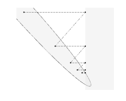
(b) ExactAlg2 ($\beta=1.30$)

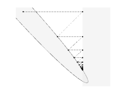
(c) ACondG-1 ($\beta=1.50$)

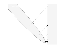
(d) ExactAlg2 ($\beta=1.50$)

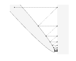
Figure 1: Behavior of ACondG-1 and ExactAlg2 algorithms on the problem of finding a point in $A\cap B$, where the sets are given as $\eqref{setA-1}$ and $\eqref{setB-1}$ with $\beta=1.30$ and $\beta=1.50$.

In the first four instances, ACondG-1 algorithm converged to a solution. In fact, in these cases, we emphasize that a feasible point has been found, not just an infeasible point satisfying the prescribed feasibility tolerance. On the other hand, ExactAlg2 failed to achieve the required feasibility tolerance $\varepsilon_{feas}=10^{-8}$ in all instances, stopping for lack of progress. For ExactAlg2, we point out that the feasibility violation measure $\min\{c_{B}(x^{k+1}),c_{A}(y^{k+1})\}$ arrived $\mathcal{O}(10^{-8})$ after 39, 45, 69, and 331 iterations for $\beta=1.30$, $1.35$, $1.40$, and $1.42$, respectively. This mean that ACondG-1 used $87.2\%$, $55.6\%$, $58.0\%$, and $63,4\%$ fewer iterations for finding a feasible point than ExactAlg2 for achieve $\mathcal{O}(10^{-8})$ in the feasibility violation measure. This seems surprising at first, because in most applications, an inexact algorithm has a low cost per iteration compared to its exact version, although the overall number of iterations tends to increase. Figures 1(a) and (b) show the behavior of ACondG-1 and ExactAlg2 algorithms for $\beta=1.30$. As can be seen, the iterates of ExactAlg2 are always at the boundary of set $A$, getting stuck at infeasible points near the intersection of the sets. In contrast, ACondG-1 goes into the interior of set $A$ approaching the intersection faster and reaching a feasible point.

In the four infeasible instances, as expected, both algorithms stopped for lack of progress reaching the same feasibility violation measure. However, as shown in Table 1, ACondG-1 required, on average, $48.7\%$ fewer iterations than ExactAlg2 to stop. Figures 1(c) and (d) show the behavior of ACondG-1 and ExactAlg2 algorithms for $\beta=1.50$. Observe that, as $k$ grows, the forcing parameters go to zero and the iterations of ACondG-1 become exact ones. This can be seen by noting that the iterates $x^{k}$, for large $k$, belong to the boundary of the ellipse.

6.2 ACondG-2 algorithm

Now we consider the problem of finding a point in the intersection of regions delimited by two ellipses. Let $A$ as in section 6.1. For defining $B$, let $z_{0}^{B}\in\mathbb{R}^{2}$ and set

$$B=\left\{z\in\mathbb{R}^{2}\colon\displaystyle\left\langle D(c,d)R(\vartheta)(z-z_{0}^{B}),~{}R(\vartheta)(z-z_{0}^{B})\right\rangle-1\leq 0\right\},$$ (37)

where $D(\cdot,\cdot)$ and $R(\cdot)$ are given as (34), $\vartheta=\pi/3$, $c=2$, and $d=2/5$.

In our tests, we defined $z_{0}^{B}=[\cdot,1/2]^{T}$ and considered different values for the first coordinate $[z_{0}^{B}]_{1}$. As for parameter $\beta$ in section 6.1, $[z_{0}^{B}]_{1}$ can be used to determine whether or not there are points at the intersection of $A$ and $B$. Table 2 shows the performance of ACondG-2 and ExactAlg3 algorithms on eight instances of the problem corresponding to the values of $[z_{0}^{B}]_{1}$ given in the first column. The remaining columns are as defined for Table 1. In each instance, the initial points were taken to be the centers of the ellipses, i.e., $x^{0}=z_{0}^{A}$ and $y^{0}=z_{0}^{B}$. Figure 2 shows the behavior of the methods in the particular cases where $[z_{0}^{B}]_{1}=2.30$ and $[z_{0}^{B}]_{1}=2.50$.

		ACondG-2			ExactAlg3
$[z_{0}^{B}]_{1}$	$A\cap B$	SC	it	$\min\{c_{B}(x^{*}),c_{A}(y^{*})\}$	SI	it	$\min\{c_{B}(x^{*}),c_{A}(y^{*})\}$
2.30		C	2	0.00D+00	L	40	2.71D-08
2.35		C	2	0.00D+00	L	127	4.60D-08
2.357		C	8	0.00D+00	L	398	7.63D-08
2.358	$\neq\varnothing$	C	155	0.00D+00	L	699	1.06D-07
2.359		L	724	1.50D-04	L	8378	7.31D-05
2.36		L	304	1.01D-03	L	1091	1.00D-03
2.40		L	23	4.01D-02	L	57	4.01D-02
2.50	$=\varnothing$	L	15	1.59D-01	L	25	1.59D-01

Table 2: Performance of ACondG-2 and ExactAlg3 algorithms on eight instances of the problem of finding a point in $A\cap B$, where the sets are given as $\eqref{setA-1}$ and $\eqref{setB-2}$.

(a) ACondG-2 ($[z_{0}^{B}]_{1}=2.30$)

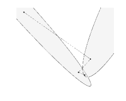
(b) ExactAlg3 ($[z_{0}^{B}]_{1}=2.30$)

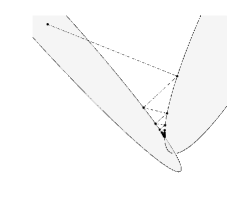
(c) ACondG-2 ($[z_{0}^{B}]_{1}=2.50$)

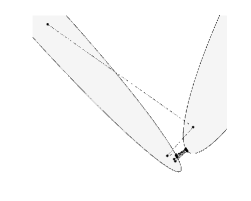
(d) ExactAlg3 ($[z_{0}^{B}]_{1}=2.50$)

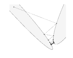
Figure 2: Behavior of ACondG-2 and ExactAlg3 algorithms on the problem of finding a point in $A\cap B$, where the sets are given as $\eqref{setA-1}$ and $\eqref{setB-2}$ with $[z_{0}^{B}]_{1}=2.30$ and $[z_{0}^{B}]_{1}=2.50$.

In the four feasible instances, ACondG-2 found a point in the intersection of $A$ and $B$ while ExactAlg3 stopped due to lack of progress. As for the exact scheme in the previous section, ExactAlg3 got stuck at infeasible points near the intersection of the sets, see Figure 2(b). We report that, with respect to ExactAlg3, the feasibility violation measure $\min\{c_{B}(x^{k+1}),c_{A}(y^{k+1})\}$ arrived $\mathcal{O}(10^{-8})$ after 35, 118, and 386 iterations for the first three instances, respectively, and $\mathcal{O}(10^{-7})$ after 526 iterations for the fourth instance. In its turn, as can be seen from Table 2, ACondG-2 found a feasible point in 2, 2, 8, and 155 iterations, respectively, showing the huge performance difference between the methods for this class of problem. As suggested by Figure 2(a), since the iterates lie in the interior of the two sets, ACondG-2 may be able to find a feasible point very quickly.

For the infeasible instances, the feasibility violation measure arrived, respectively, $\mathcal{O}(10^{-4})$, $\mathcal{O}(10^{-3})$, $\mathcal{O}(10^{-2})$, and $\mathcal{O}(10^{-1})$ after 33, 5, 3, and 2 iterations for ACondG-2 and after 82, 15, 5, and 2 for ExactAlg3. This shows that, for the chosen set of problems, ACondG-2 approaches the nearest region between $A$ and $B$ faster than ExactAlg3, see Figures 2(c) and (d). On average, ACondG-2 required $65.7\%$ fewer iterations than ExactAlg3 for stopping due to lack of progress. On the other hand, in some instances, ExactAlg3 obtained a final iterate with a smaller feasibility violation measure. This can be explained by the fact that algorithms use different numerical approaches to calculate projections.

Last but not least, the performance of the methods presented throughout the numerical results section should be taken as an illustration of the capabilities of the introduced methods with respect to their exact counterparts, taking into account that they correspond to small problems with specific structures. More precise conclusions should be made after numerical experiments using problems of different classes and scales.

7 Conclusions

In the present paper, we proposed a new method to solve Problem (1) by combining CondG method with the alternate directions method. As suggested by the numerical experiments, the proposed method seems promising. Let us highlight some aspects observed during the numerical tests. In the chosen set of test problems, the inexact methods performed fewer iterations than the exact ones. In particular, whenever the intersection of the involved sets has a nonempty interior, the methods converged in a finite number of iterations. These phenomena deserve further investigations. It would also be interesting to extend ACondG method to the convex feasibility problem with multiple involved sets. Finally, the CondG method can also be used to design inexact versions of several projection methods, including but not limited to averaged projections method [32], Han’s method [26] (see also [2]) or more generally Dykstra’s alternating projection method [2]. For more variants of projections methods see [13, Section III]. For instance, one inexact version of averaged projection method for two sets is stated as follows:

Step 0.

Let $(\lambda_{k})_{k\in\mathbb{N}}$, $(\gamma_{k})_{k\in\mathbb{N}}$, and $(\theta_{k})_{k\in\mathbb{N}}$ be sequences of nonnegative real numbers and $\varphi_{k}:=\varphi_{\gamma_{k},\theta_{k},\lambda_{k}}$, as defined in (2). Let $x_{0}\in A$, $y_{0}\in B$, and set $z_{0}:=(x_{0}+y_{0})/2$. Initialize $k\leftarrow 0$.

Step 1.

If $z^{k}\in A\cap B$, then stop.

Step 2.

Using Agorithm 1, compute $\mbox{CondG${}_{A}$}\,(\varphi_{k},x^{k},z^{k})$ and $\mbox{CondG${}_{B}$}\,(\varphi_{k},y^{k},z^{k})$ and set the next iterate $z^{k+1}$ as

$$z^{k+1}:=\frac{1}{2}\left[\mbox{CondG${}_{A}$}\,(\varphi_{k},x^{k},z^{k})+\mbox{CondG${}_{B}$}\,(\varphi_{k},y^{k},z^{k})\right].$$

Step 3.

Set $k\leftarrow k+1$, and go to Step 1.

Algorithm 4 Averaged projection method with inexact projections onto two sets

References

- [1] H. H. Bauschke and J. M. Borwein, On the convergence of von Neumann’s alternating projection algorithm for two sets, Set-Valued Anal., 1 (1993), pp. 185–212.
- [2] H. H. Bauschke and J. M. Borwein, Dykstra’s alternating projection algorithm for two sets, J. Approx. Theory, 79 (1994), pp. 418–443.
- [3] H. H. Bauschke and J. M. Borwein, On projection algorithms for solving convex feasibility problems, SIAM Rev., 38 (1996), pp. 367–426.
- [4] H. H. Bauschke and P. L. Combettes, A weak-to-strong convergence principle for Fejér-monotone methods in Hilbert spaces, Math. Oper. Res., 26 (2001), pp. 248–264.
- [5] H. H. Bauschke and P. L. Combettes, Convex analysis and monotone operator theory in Hilbert spaces, CMS Books in Mathematics/Ouvrages de Mathématiques de la SMC, Springer, New York, 2011.
- [6] A. Beck and M. Teboulle, A conditional gradient method with linear rate of convergence for solving convex linear systems, Math. Methods Oper. Res., 59 (2004), pp. 235–247.
- [7] E. G. Birgin and J. M. Martínez, Practical augmented Lagrangian methods for constrained optimization, SIAM, 2014.
- [8] L. M. Brègman, Finding the common point of convex sets by the method of successive projection, Dokl. Akad. Nauk SSSR, 162 (1965), pp. 487–490.
- [9] A. Cegielski, S. Reich, and R. Zalas, Regular sequences of quasi-nonexpansive operators and their applications, SIAM J. Optim., 28 (2018), pp. 1508–1532.
- [10] Y. Censor and A. Cegielski, Projection methods: an annotated bibliography of books and reviews, Optimization, 64 (2015), pp. 2343–2358.
- [11] W. Cheney and A. A. Goldstein, Proximity maps for convex sets, Proc. Amer. Math. Soc., 10 (1959), pp. 448–450.
- [12] K. L. Clarkson, Coresets, sparse greedy approximation, and the Frank-Wolfe algorithm, ACM Trans. Algorithms, 6 (2010), pp. Art. 63, 30.
- [13] P. L. Combettes, The foundations of set theoretic estimation, Proceedings of the IEEE, 81 (1993), pp. 182–208.
- [14] P. L. Combettes, The convex feasibility problem in image recovery, Advances in imaging and electron physics- Vo. 95, P. Hawkes, ed., Academic Press, New York,, (1996), pp. 155–270.
- [15] P. L. Combettes, Hard-constrained inconsistent signal feasibility problems, EEE Trans. Signal Process., 47, (1999), pp. 2460–2468.
- [16] P. L. Combettes, Quasi-Fejérian analysis of some optimization algorithms, in Inherently parallel algorithms in feasibility and optimization and their applications (Haifa, 2000), vol. 8 of Stud. Comput. Math., North-Holland, Amsterdam, 2001, pp. 115–152.
- [17] R. Díaz Millán, S. B. Lindstrom, and V. Roshchina, Comparing averaged relaxed cutters and projection methods: Theory and examples, Special Springer Volume commemorating Jon Borwein, Springer Proceedings in Mathematics Statistics, to appear, (2019).
- [18] D. Drusvyatskiy and A. S. Lewis, Local linear convergence for inexact alternating projections on nonconvex sets, Vietnam J. Math., 47 (2019), pp. 669–681.
- [19] J. C. Dunn, Convergence rates for conditional gradient sequences generated by implicit step length rules, SIAM J. Control Optim., 18 (1980), pp. 473–487.
- [20] M. Frank and P. Wolfe, An algorithm for quadratic programming, Nav. Res. Log., (1956), pp. 95–110.
- [21] R. M. Freund and P. Grigas, New analysis and results for the Frank-Wolfe method, Math. Program., 155 (2016), pp. 199–230.
- [22] M. Fukushima, A modified Frank-Wolfe algorithm for solving the traffic assignment problem, Transportation Res. Part B, 18 (1984), pp. 169–177.
- [23] M. Fukushima, A relaxed projection method for variational inequalities, Math. Programming, 35 (1986), pp. 58–70.
- [24] D. Garber and E. Hazan, Faster rates for the frank-wolfe method over strongly-convex sets, Proceedings of the 32Nd International Conference on International Conference on Machine Learning - Volume 37, (2015), pp. 541–549.
- [25] M. L. N. Gonçalves and J. G. Melo, A Newton conditional gradient method for constrained nonlinear systems, J. Comput. Appl. Math., 311 (2017), pp. 473–483.
- [26] S.-P. Han, A successive projection method, Math. Programming, 40 (1988), pp. 1–14.
- [27] R. Hesse, D. R. Luke, and P. Neumann, Alternating projections and Douglas-Rachford for sparse affine feasibility, IEEE Trans. Signal Process., 62 (2014), pp. 4868–4881.
- [28] A. N. Iusem, A. Jofré, and P. Thompson, Incremental constraint projection methods for monotone stochastic variational inequalities, Math. Oper. Res., 44 (2019), pp. 236–263.
- [29] M. Jaggi, Revisiting frank-wolfe: Projection-free sparse convex optimization, Proceedings of the 30th International Conference on International Conference on Machine Learning - Volume 28, ICML’13 (2013), pp. I–427–I–435.
- [30] G. Lan and Y. Zhou, Conditional gradient sliding for convex optimization, SIAM J. Optim., 26 (2016), pp. 1379–1409.
- [31] E. S. Levitin and B. T. Poljak, Minimization methods in the presence of constraints, USSR Computational mathematics and mathematical physics, 6 (1966), pp. 1–50.
- [32] A. S. Lewis, D. R. Luke, and J. Malick, Local linear convergence for alternating and averaged nonconvex projections, Found. Comput. Math., 9 (2009), pp. 485–513.
- [33] R. Luss and M. Teboulle, Conditional gradient algorithms for rank-one matrix approximations with a sparsity constraint, SIAM Rev., 55 (2013), pp. 65–98.
- [34] J. von Neumann, Functional Operators. II. The Geometry of Orthogonal Spaces, Annals of Mathematics Studies, no. 22, Princeton University Press, Princeton, N. J., 1950.