The disordered lattice free field pinning model approaching criticality

Abstract.

We continue the study, initiated in [21], of the localization transition of a lattice free field $\phi=(\phi(x))_{x\in{\mathbb{Z}}^{d}}$, $d\geq 3$, in presence of a quenched disordered substrate. The presence of the substrate affects the interface at the spatial sites in which the interface height is close to zero. This corresponds to the Hamiltonian

$$\sum_{x\in{\mathbb{Z}}^{d}}(\beta\omega_{x}+h)\delta_{x},$$

where $\delta_{x}=\mathbf{1}_{[-1,1]}(\phi(x))$, and $(\omega_{x})_{x\in{\mathbb{Z}}^{d}}$ is an IID centered field. A transition takes place when the average pinning potential $h$ goes past a threshold $h_{c}(\beta)$: from a delocalized phase $h<h_{c}(\beta)$, where the field is macroscopically repelled by the substrate, to a localized one $h>h_{c}(\beta)$ where the field sticks to the substrate. In [21] the critical value of $h$ is identified and it coincides, up to the sign, with the $\log$-Laplace transform of $\omega=\omega_{x}$, that is $-h_{c}(\beta)=\lambda(\beta):=\log{\mathbb{E}}[e^{\beta\omega}]$. Here we obtain the sharp critical behavior of the free energy approaching criticality:

$$\lim_{u\searrow 0}\frac{\textsc{f}(\beta,h_{c}(\beta)+u)}{u^{2}}=\frac{1}{2\,\mathrm{Var}\left(e^{\beta\omega-\lambda(\beta)}\right)}.$$

Moreover, we give a precise description of the trajectories of the field in the same regime: the absolute value of the field is $\sqrt{2\sigma_{d}^{2}|\log(h-h_{c}(\beta))|}$ to leading order when $h\searrow h_{c}(\beta)$ except on a vanishing fraction of sites ($\sigma_{d}^{2}$ is the single site variance of the free field).
2010 Mathematics Subject Classification: 60K35, 60K37, 82B27, 82B44
Keywords: Lattice Free Field, Disordered Pinning Model, Localization Transition, Critical Behavior, Disorder Relevance, Multiscale Analysis

1. Introduction

1.1. Disorder and critical phenomena: an overview, till the free field pinning case

A fundamental issue in statistical mechanics is the effect of disorder, synonymous of random environment and (with more old fashioned language) of impurities, on phase transitions. The issue is very general and applies to any statistical model that exhibits a phase transition: in mathematical terms, a phase transition happens at a given value, called critical, of a parameter (the temperature, an external field,$\ldots$) when one or more observables on the system have a singular, i.e. non-analytic, behavior in the parameter we are considering, at the critical value. The behavior of systems approaching criticality is particularly interesting because of the appearance of universal behaviors that are, to a certain extent, characterized in terms of critical exponents (e.g. [16, 17]). Consider now a spatially homogeneous model, i. e. a model in which the interactions are translation invariant, that has a phase transition. If we modify the interactions by perturbing them in a spatially random way, we obtain, for every realization of the randomness, a different non homogeneous model (that we call disordered): does the phase transition survive to the introduction of this randomness? And, if it does, is the nature of the transition affected? That is, are the critical exponents the same as in the homogeneous case?

In spite of the general nature of the problem, phase transitions and critical phenomena are under control only for particular homogeneous models, or classes of homogeneous models. The most famous one, and first (nontrivial) one to be solved (in 1944, by Lars Onsager) is the two dimensional Ising model (on square lattice, with ferromagnetic interactions and in absence of external field): this model has been at the heart of the activity of a large community of researchers since. A part of this community, mostly on the physical side, focused on the issue that interests us, that is whether Onsager’s results withstand the introduction of disorder, for example a small amount of disorder. And it is precisely in the Ising model context that A. B. Harris [23] took an approach to this question that turned out to be very successful in the physical community. Harris’ approach is based on the renormalization group and can be summed up (in a vague but hopefully evocative fashion) by saying that one has to consider what is the effect of the renormalization transformation on the disorder when the system is close to criticality. If the renormalization tends to suppress the disorder then one expects that on large scale the disorder will be irrelevant, and the critical phenomenon will not be affected by the disorder. On the other hand, if disorder is enhanced by the renormalization group transformation, one generically expects that the critical behavior is affected by the disorder, that is therefore dubbed relevant. The success of Harris’ arguments is in part due to the fact that he was able to make them boil down to a very simple criterion, called Harris criterion.

In spite of the fact that these ideas are around since at least 45 years and that they are commonly applied in physics, from the mathematical viewpoint the understanding of the Harris criterion is very limited, notably for the original example of the two dimensional Ising model (see [20, Ch. 5] for a review). Only more recently (see [2, 20] and references therein) the Harris criterion prediction has been proven in full for a class of statistical mechanics models: the pinning models.

Keeping at a very informal level, pinning models can be visualized as interface pinning models. An effective $d+1$ dimensional interface is modeled by considering a random function from ${\mathbb{Z}}^{d}$ to ${\mathbb{R}}$ (or to ${\mathbb{Z}}$): examples include the Lattice Free Field (LFF) or other gradient fields like the massless fields or the Solid On Solid (SOS) models (see e.g. [17, Ch.8] for an introduction to the LFF or [18, 29, 30] for more advanced material). In $d=1$ these interface models just reduce to random walk models. The pinning potential is a reward that is introduced via an energy term (we are taking a Gibbsian viewpoint of the probability law of the model) that rewards or penalizes the visit to level zero (if the interface takes values in ${\mathbb{Z}}$) or a neighborhood of level $0$ (if the interface takes values in ${\mathbb{R}}$): we call these visits contacts. The intensity of the reward is parametrized by a variable $h$, and it can become a penalization if we change the sign of $h$. In the disordered case we simply make $h$ depend on $x$: the parametrization we choose is $h+\beta\omega_{x}$, where $(\omega_{x})_{x\in{\mathbb{Z}}^{d}}$ are IID centered random variables (with suitable integrability properties), and $\beta\geq 0$.

As already understood in [15], the $d=1$ model has an intrinsic independence structure that allows in particular a generalization of the model that turns out to be very important in the Harris criterion perspective: in mathematical terms the model can be rewritten (for every value of $d$) just in terms of the point process represented by the location of the contacts and if $d=1$ the contact set is just a renewal process (if the interface takes values in ${\mathbb{Z}}$, otherwise it is a Markov renewal process)[19, 20]. This is not only precious in solving the model – notably, the $d=1$ homogeneous case is exactly solvable – but it offers an immediate natural generalization to the large class of renewal pinning models. So for $d=1$, in the generalized context we just hinted to, one can obtain models for which Harris criterion predicts disorder irrelevance and other ones for which it predicts disorder relevance. We refer to [19, 20] for the large literature on $1+1$ dimensional pinning and renewal pinning. But we want to stress that if the irrelevant disorder results are very satisfactory (and they are proven exactly when Harris criterion predicts irrelevance), relevant disorder results are much weaker. This is not surprising: Harris criterion does not bear information about what the critical behavior is, if disorder is relevant. Nevertheless, it has been shown that, when the Harris criterion predicts disorder relevance, the critical behavior is not the same as the one of the homogeneous model. What the disordered critical behavior really is remains mathematically a fully open issue. Substantial progress on this problem has been recently achieved, but not for the pinning models itself: the critical behavior of a relevant disorder case for one class of copolymer pinning models and of a simplified version of the hierarchical pinning model have been identified respectively in [1] and in [9].

The $d>1$ case is a priori more difficult to handle and, above all, the contact set does not enjoy the independence (renewal) structure of the $d=1$ case: it is replaced by a more geometric spatial Markov property. The problem has been attacked in [11, 21, 24] by using the LFF as interface model: the homogeneous model turns out to be solvable (or, at least, has a certain degree of solvability) and, as far as the questions we raise, in a rather elementary way. In particular, it displays a delocalization to localization transition at a critical value $h_{c}$, as $h$ grows. It is also rather straightforward to see that this transition survives when disorder is introduced, that is for $\beta>0$. A peculiar feature of this transition is that $h_{c}$, or $h_{c}(\beta)$ when $\beta>0$, separates the regime $h<h_{c}(\beta)$ in which the contact fraction is zero (delocalized regime), and the regime $h>h_{c}(\beta)$ in which the contact fraction is positive (localized regime).

What is instead much less obvious [21, 24] is the identification of the critical value $h_{c}(\beta)$, along with estimates on the contact fraction of the system that show that disorder is relevant in all dimensions $d\geq 2$. In particular, for $d\geq 3$, the case on which we focus here, we have proven in [21] that the contact fraction approaching criticality, i.e. $h\searrow h_{c}(\beta)$, is bounded above and below by $h-h_{c}(\beta)$ times a positive constant (different for lower and upper bound). This result has been established only for Gaussian disorder, while for more general disorder a lower bound of $(h-h_{c}(\beta))^{c}$, $c>1$ is a constant that depends on $d$. Therefore the contact fraction is (Lipschitz) continuous for $\beta>0$ and this is sufficient to infer that disorder is relevant. In fact for $\beta=0$ the contact fraction is discontinuous at the critical value.

The content of the work we present now is:

1. showing that, when $h\searrow h_{c}(\beta)$, the contact fraction behaves like $h-h_{c}(\beta)$ times a constant that depends on $\beta$ and on the law of the disorder, on which we make only integrability assumptions;

2. providing precise path estimates in the same limit. That is, describing the trajectories on which the system concentrates near criticality.

Precise contact fraction estimates like the ones in point (1) typically demand at least a heuristic understanding of the path behavior of point (2). Therefore in our context they demand a good understanding of the localization mechanism for the disordered system near criticality. This is one of the main achievements of our analysis.

On the other hand, the step from (1) to (2) is by no mean evident and, as a matter of fact, it is technically the most demanding part of our analysis, involving in particular a full multiscale analysis.

1.2. The model’s building blocks: Lattice Free Field and disorder

We set $\Lambda_{N}:=\llbracket 0,N\rrbracket^{d}$, $d\geq 3$, $N\in{\mathbb{N}}$, and consider the centered free field on this set. That is, we consider a Gaussian family of centered random variables $(\phi(x))_{x\in{\mathbb{Z}}^{d}}$, whose law is denoted by ${\mathbf{P}}_{N}$, with ${\mathbf{E}}_{N}[\phi(x)\phi(y)]:=G_{N}(x,y)$ where $G_{N}(\cdot,\cdot)$ is the Green function associated with the simple symmetric random walk on ${\mathbb{Z}}^{d}$ killed upon exiting $\mathring{\Lambda}_{N}:=\llbracket 1,N-1\rrbracket^{d}$. More explicitly, if $P_{x}$ denotes the distribution law of a simple symmetric continuous time random walk $(S_{t})_{t\geq 0}$ with jump rate one in each direction and initial condition $S_{0}=x$, then

$$G_{N}(x,y)\,=\,E_{x}\left[\int_{0}^{\tau_{N}}\mathbf{1}_{\{S_{t}=y\}}\mathrm{d}t\right]\,,\ \ \text{ with }\ \ \tau_{N}:=\inf\left\{t>0:\,S_{t}\notin\mathring{\Lambda}_{N}\right\}\,.$$ (1.1)

It is well known that the Green function $G(\cdot,\cdot)$ of the simple random walk without killing (obtained by replacing $\tau_{N}$ in (1.1) by $\infty$) exists for $d\geq 3$. We let ${\mathbf{P}}$ denote the law of the Gaussian field on ${\mathbb{Z}}^{d}$ with covariance $G(\cdot,\cdot)$. We also set $\sigma_{d}^{2}:=G(0,0)$.

Let us recall from now some well known random walk estimates in transient dimensions that we will repeatedly use. First of all $\lim_{x\to\infty}|x|^{d-2}G(0,x)$ exists and it is positive, so in particular we can find $C_{d}>1$ such that for every $x\neq 0$

$$C_{d}^{-1}|x|^{2-d}\,\leq\,G(0,x)\,\leq\,C_{d}|x|^{2-d}\,.$$ (1.2)

Moreover

$$0\leq\,G(0,0)-G_{N}(0,0)\,=\,O\left(1/N^{d-2}\right)\,,$$ (1.3)

and, always aiming at comparing the Green function and its killed version, we have that for any sequence $z_{N}$ such that $\lim_{N\to\infty}\mathrm{dist}(z_{N},\Lambda^{\complement}_{N})=\infty$ (e.g. $z_{N}:=\lceil N/2\rceil(1,1,\dots,1)$) for every $x,y\in{\mathbb{Z}}^{d}$

$$G(x,y)=G(0,y-x)=\lim_{N\to\infty}G_{N}(x+z_{N},y+z_{N})\,.$$ (1.4)

Of course, for $x\in{\mathbb{Z}}^{d}$ and $A\subset{\mathbb{Z}}^{d}$, $\mathrm{dist}(x,A):=\min_{y\in A}|x-y|$ and we make the choice (irrelevant in most of the cases, but of some importance for some geometric constructions) that $|\cdot|$ denotes the $\ell_{1}$ distance in ${\mathbb{Z}}^{d}$, that is $|x|=\sum_{j=1}^{d}|x_{j}|$ (but for $x\in{\mathbb{R}}^{d}$ we use $|x|$ for the Euclidean norm).

The disorder, or random environment, $(\omega_{x})_{x\in{\mathbb{Z}}^{d}}$ is a family of IID random variables, ${\mathbb{P}}$ is its law. Free field and disorder are independent. We assume that

$$\lambda(s)\,:=\,\log{\mathbb{E}}\left[\exp\left(s\omega\right)\right]\,<\,\infty\ \ \text{ for every }s\in{\mathbb{R}}\,,$$ (1.5)

and that $\lambda^{\prime}(\cdot)$ is not a constant, i. e. $\omega$ is not a constant. In (1.5) we have dropped the index $x$ for obvious reasons. Without loss of generality we assume ${\mathbb{E}}[\omega]=0$: this is largely irrelevant because $\omega$ appears in the model in the form $\beta\omega-\lambda(\beta)$ which is invariant under the transformation $\omega\mapsto\omega+$constant. However, ${\mathbb{E}}[\omega]=0$ assures that $\lambda(\cdot)$ is increasing on the positive semi-axis and decreasing in the negative one, and this is practical.

The generalization of the results to the case in which we assume (1.5) only, say, for $|s|$ smaller than a constant is not straightforward. The full hypothesis (1.5) is used for a cut-off estimate, see Section A.2, that is probably not necessary but it does not appear to be easy to circumvent. On the other hand, a part of the main results (notably, the probability upper bound) can be obtained under very mild hypothesis on the lower (negative) tail of $\omega$, in particular for this results (1.5) is exploited only for $s>0$. For sake of readability we will make precise this aspect only in the technical part of the work (see Remark 2.1).

1.3. The disordered lattice free field pinning model

The model we consider is the disordered pinning model based on the LFF with law ${\mathbf{P}}_{N}$. For $\beta\geq 0$ and $h\in{\mathbb{R}}$ we set

$$\frac{\mathrm{d}{\mathbf{P}}_{N,\omega,\beta,h}}{\mathrm{d}{\mathbf{P}}_{N}}(\phi)\,:=\,\frac{1}{Z_{N,\omega,\beta,h}}e^{\sum_{x\in\Lambda_{N}}(\beta\omega_{x}-\lambda(\beta)+h)\delta_{x}}\,,\ \ \text{ with }\ \delta_{x}:=\mathbf{1}_{[-1,1]}(\phi(x))\,,$$ (1.6)

where of course $Z_{N,\omega,\beta,h}$ is the normalization constant (or partition function)

$$Z_{N,\omega,\beta,h}\,:=\,{\mathbf{E}}_{N}\left[\exp\left(\sum_{x\in\Lambda_{N}}(\beta\omega_{x}-\lambda(\beta)+h)\delta_{x}\right)\right]\,.$$ (1.7)

We will often use the notation

$${\mathcal{F}}_{A}^{\phi}\,:=\,\sigma(\phi(x):\,x\in A)\,.$$ (1.8)

Note that ${\mathbf{P}}_{N,\omega,\beta,h}$ does not change if we replace summing over $x\in\Lambda_{N}$ with $x\in\mathring{\Lambda}_{N}$ or any other set $\Lambda$, $\mathring{\Lambda}_{N}\subset\Lambda\subset\Lambda_{N}$. $Z_{N,\omega,\beta,h}$ is affected by such a change, but only in a trivial way and, in particular, the free energy density (that we will simply call free energy)

$$\textsc{f}(\beta,h)\,:=\,\lim_{N\to\infty}\frac{1}{|\Lambda_{N}|}{\mathbb{E}}\log Z_{N,\omega,\beta,h}\,,$$ (1.9)

is clearly not affected either. The proof of the existence of the limit in (1.9) can be found in [11]: the argument is based on the almost super-additive behavior of the sequence $({\mathbb{E}}\log Z_{N,\omega,\beta,h})_{N\in{\mathbb{N}}}$. We will come back to to this issue (see Proposition 3.2) because a sharp super-additive behavior for a modified partition function, that gives rise to the same free energy, is going to be important, notably for the lower bound on the free energy in Section 3. Here are some basic, but crucial, properties of the free energy (see the introduction of [21] for full details):

• The map $(\beta,h)\mapsto\textsc{f}(\beta,h)$ is convex, moreover it is non decreasing in $h\in{\mathbb{R}}$ for $\beta$ fixed and in $\beta\geq 0$ for $h$ fixed;

• The inequality $\textsc{f}(\beta,h)\geq 0$ holds because of the rough entropic repulsion estimate $\log{\mathbf{P}}_{1}(\phi(x)>1$ for every $x\in\mathring{\Lambda}_{N})=o(|\Lambda_{N}|)$ which is easily derived by exploiting the continuum symmetry of the LFF [28];

• By Jensen’s inequality, we have $\textsc{f}(\beta,h)\leq\textsc{f}(0,h)$ (annealed bound)  .

The convexity and monotonicity properties in $h$ lead to identifying

$$h_{c}(\beta)\,:=\,\inf\{h:\,\textsc{f}(\beta,h)>0\}\,=\,\inf\{h:\,\partial_{h}\textsc{f}(\beta,h)>0\}\,,$$ (1.10)

as a critical point, provided that $h_{c}(\beta)\not=\pm\infty$. Elementary estimates lead to excluding $h_{c}(\beta)\not=\pm\infty$, but much more than that is true: in [21] is shown that $h_{c}(\beta)=0$ for every $\beta\geq 0$. Again we refer to the introduction of [21] for full details, but we stress that establishing $h_{c}(\beta)\geq 0$ is a rather straightforward consequence of comparison with the model without disorder: of course $\textsc{f}(0,h)=0$ for $h\leq 0$ and a very moderate amount of work leads to

$$\textsc{f}(0,h)\stackrel{{\scriptstyle h\searrow 0}}{{\sim}}c_{d}h\,,\ \ \text{ with }c_{d}\,:=\,{\mathbf{P}}(\phi(0)\in[-1,1])\,=\,P(\sigma_{d}{\mathcal{N}}\in[-1,1])\,,$$ (1.11)

and ${\mathcal{N}}$ is our notation for a standard Gaussian variable. In particular (1.11) yields $h_{c}(0)=0$ and, in turn, from the annealed bound we obtain $h_{c}(\beta)\geq h_{c}(0)$. Remark also that from the annealed bound we extract $\textsc{f}(\beta,h)\leq ch$, for any $c>c_{d}$ and $h>0$ small. However this result is poor precisely because disorder is relevant for this model: the main result in [21] is that if $\omega_{x}$’s are standard Gaussian variables then for $h\in(0,1)$

$$C_{-}(\beta)h^{2}\,\leq\,\textsc{f}(\beta,h)\,\leq\,C_{+}(\beta)h^{2}\,,$$ (1.12)

with $C_{\pm}(\beta)>0$ satisfying $\lim_{\beta\searrow 0}\beta^{2}C_{\pm}(\beta)=c_{\pm}>0$, and $c_{-}<c_{+}$. We remark that, exploiting the convexity of $\textsc{f}(\beta,\cdot)$ and the fact that $\partial_{h}\log Z_{N,\omega,\beta,h}={\mathbf{E}}_{N,\omega,\beta,h}[\sum_{x\in\Lambda_{N}}\delta_{x}]$, one readily obtains that the infinite volume contact density $\rho(\beta,h):=\lim_{N}\rho_{N}(\beta,h)$, with $\rho_{N}(\beta,h):={\mathbf{E}}_{N,\omega,\beta,h}\left[\sum_{x\in\Lambda_{N}}\delta_{x}/{|\Lambda_{N}|}\right]$, exists except possibly for countably many values of $h$: the non decreasing function $\rho(\beta,\cdot)$ may have jumps and, when it does, its value is not well defined at the jump. In order to avoid this nuisance we extend the definition of $\rho(\beta,h)$ choosing the right continuous version of $\rho(\beta,\cdot)$ (the results that follow are exactly the same for the left continuous version). From (1.12) one easily obtains

$$2C_{-}(\beta)h\,\leq\,\rho(\beta,h)\,\leq\,4C_{+}(\beta)h\,,$$ (1.13)

for every $h\in(0,1)$ for the lower bound and for every $h\in(0,1/2)$ for the upper bound, see Remark 1.3.

Also results for general disorder are given in [21], but they are rougher than (1.12), in the sense that, in the lower bound in (1.12), $h^{2}$ is replaced by $h$ to a large power. Nevertheless, the results we just cited show that disorder is relevant for the model we consider: the critical behavior changes when disorder is switched on.

1.4. The main results

The first main result of this paper is a sharp version of (1.12), valid for general disorder distribution. We prove that $\textsc{f}(\beta,h)$ is asymptotically proportional to $h^{2}$ when $h\searrow 0$ and identify the value of the constant in front of $h^{2}$.

Theorem 1.1.

For every $\beta>0$ we have that

$$\textsc{f}(\beta,h)\stackrel{{\scriptstyle h\searrow 0}}{{\sim}}\chi(\beta)h^{2}\,,$$ (1.14)

with

$$\chi(\beta)\,:=\,\frac{1}{2\mathrm{Var}(e^{\beta\omega_{x}-\lambda(\beta)})}=\frac{1}{2(e^{\lambda(2\beta)-2\lambda(\beta)}-1)}\,.$$ (1.15)

Theorem 1.1 sums up quantitative upper and lower bounds (Propositions 2.2 and 3.1 respectively) that bear more information on the rate of convergence of (1.14). Moreover one easily extracts from (1.14) the following asymptotic equivalence on the contact fraction (cf. Remark 1.3)

$$\rho(\beta,h)\stackrel{{\scriptstyle h\searrow 0}}{{\sim}}2\chi(\beta)h\,.$$ (1.16)

Of course (1.16) gives already a precise information on the behavior of the trajectories with law ${\mathbf{P}}_{N,\omega,\beta,h}$ in the infinite volume limit and near criticality. Our second main result, Theorem 1.2 below, goes much farther in this direction.

Recall, cf. the end of Section 1.2, that $\sigma_{d}$ denotes the standard deviation of the one site marginal of the infinite volume LFF. The following result shows that asymptotically most of the points in the field are located around height $\sigma_{d}\sqrt{2\log(1/h)}$.

Theorem 1.2.

Given $\varepsilon>0$, there exists $h_{0}(\varepsilon)>0$ such that for every $h\in(0,h_{0}(\varepsilon))$ we can find $c:=c(\varepsilon,h)>0$ and $N_{0}:=N_{0}(\omega,\varepsilon,h)$, with ${\mathbb{P}}(N_{0}<\infty)=1$, such that ${\mathbb{P}}(\mathrm{d}\omega)$-a.s. we have for $N>N_{0}$

$${\mathbf{P}}_{N,\omega,\beta,h}\left(\left|\left\{{x\in\Lambda_{N}}:\,\left|{|\phi(x)|}{{(\log(1/h))^{-1/2}}}-\sqrt{2}\,\sigma_{d}\right|>\varepsilon\right\}\right|\,\geq\,\varepsilon N^{d}\right)\,\leq\,e^{-cN^{d}}\,.$$ (1.17)

This result considerably refines previous estimates obtained on the trajectories. In [21] it was only proved that typically most point are above height $c_{d}\sqrt{\log(1/h)}$ (in absolute value) for an explicit non-optimal constant $c_{d}$.

Remark 1.3.

The arguments to go from (1.12) to (1.13) and from (1.14) to (1.16) are standard, but we sketch them here. If $f:[0,\infty)\to[0,\infty)$ is a convex increasing function such that $C_{1}h^{2}\leq f(h)\leq C_{2}h^{2}$ for $h\in[0,h_{0}]$, with $C_{1}>0$, then convexity directly yields $\partial f(h)\geq 2C_{1}h$. Here $\partial f(\cdot)$ is either the upper or the lower differential of $f$. Since $\partial f(\cdot)$ is non decreasing we have that, for every $h\in[0,h_{0}/2]$, $\partial f(u)\geq\partial f(h)\mathbf{1}_{[h,\infty)}(u)$. By integrating from $0$ to $2h$ this inequality we obtain $\partial f(h)h\leq f(2h)\leq 4C_{2}h^{2}$, that is $\partial f(h)\leq 4C_{2}h$. On the other hand, if $C_{2}=(1+\varepsilon^{2})C_{1}$, then by integrating $\partial f(u)\geq 2C_{1}u\mathbf{1}_{(0,h)}(u)+\partial f(h)\mathbf{1}_{[h,\infty)}(u)$ for $u$ going from $0$ to $(1+\varepsilon)h\leq h_{0}$ we obtain that $\partial f(h)\leq 2C_{1}h(1+3\varepsilon)$, for $\varepsilon\in[0,1]$.

1.5. Discussion of the results, relevant literature and organization of the paper

Localization strategy and sketch of proofs

A key point and one of the main novelty of our work is that we identify the localization mechanism. And this mechanism is crucially suggested by the argument for the upper bound on the free energy. The upper bound we give is a universal bound: it holds for an arbitrary random contact set. More explicitly: the partition function (1.7) depends only on the random field $(\delta_{x})_{x\in\mathring{\Lambda}_{N}}$ or, equivalently, on the random set $\{x\in\mathring{\Lambda}_{N}:\,\delta_{x}=1\}$, and we give an upper bound on the free energy density not only for $\delta_{x}=\mathbf{1}_{[-1,1]}(\phi(x))$ with $\phi$ the LFF on $\Lambda_{N}$ with zero boundary conditions, but with an arbitrary law of $(\delta_{x})_{x\in\mathring{\Lambda}_{N}}$. Moreover this bound is saturated by choosing $(\delta_{x})_{x\in\mathring{\Lambda}_{N}}$ IID Bernoulli variables of a parameter $p$ chosen to be the value $p(\beta,h)$ that maximizes the function

$$p\mapsto{\mathbb{E}}\log\left(1+p\left(\exp\left(\beta\omega-\lambda(\beta)+h\right)\right)\right)\,.$$ (1.18)

In the limit $h\searrow 0$ we obtain that $p(\beta,h)\sim 2\chi(\beta)h$. Why should the contact set that we obtain from the LFF be close to saturating this bound too? At a heuristic level the reason is a combination of two well known facts on the LFF:

1. the continuum symmetry of the LFF that makes rigid vertical translations of the interface little expensive (this is of course very much in the logic of the entropic repulsion phenomena [4, 5, 12, 13, 28])

2. large excursions of the LFF have very mild correlations (an issue underlying [5, 13] and developed in detail in [10]).

This suggests the following behavior for the field when $h>0$ is small: the field shifts away from level $0$, precisely it shifts to a level $u(\beta,h)$, or $-u(\beta,h)$, so that the probability that $\phi(x)\sim{\mathcal{N}}(\sigma_{d}^{2},\pm u(\beta,h))$ belongs to $[-1,1]$ is equal to $p(\beta,h)$. As the reader might expect in view of Theorem 1.2, it turns out that $u(\beta,h)$ is asymptotically equivalent to the square root of $2\sigma_{d}^{2}\log(1/h)$.

To substantiate this localization strategy we need to provide a lower bound. This is achieved by considering the field with boundary conditions $u(\beta,h)$ – the value of the free energy does not depend on on this choice – and via a two step decomposition of the LFF that is in the spirit of several earlier works: in three or more dimension the LFF can be written as the superposition of a field with small variance, and spatially power law decaying covariance, and a field that accounts for almost all the variance of the original field, but with exponentially decaying covariance: it is for example the case of the decomposition of the field theory literature [7, 16] in which $G=G_{\epsilon}+(G-G_{\epsilon})$ where $G_{\epsilon}$ is the Green function of a walk with a rate of death $\epsilon>0$, see [13, Sec. 4] for a probabilistic presentation. We propose instead a decomposition that is much more geometrically structured: we write $\phi$ as a power law correlated field (with small variance) plus independent fields that are compactly supported over boxes (i.e. hypercubes). The boxes have edge length proportional to $h^{-c}$, $c>0$ a small constant, and they overlap only near the boundary. Recalling that the boundary of the LFF is set to height $u(\beta,h)$, hence the mean of the field is $u(\beta,h)$, in each one of these boxes we typically expect no contact, because the contact density is proportional to $h$ and the volume of each box is $h^{-cd}$ (and $c$ is small, in particular $c<1/d$). On this scale we are able to perform an accurate analysis that shows that the leading contribution to the free energy in each of these boxes is given by configurations with one or two contacts. The errors introduced by the power law correlated field (with small variance) and by the overlap regions turn out to be higher order corrections.

The next step is proving that the trajectories of the field behave like what is suggested by the asymptotic of the free energy and its proof. This is a matter of proving upper and lower bounds on the height of the field with law ${\mathbf{P}}_{N,\omega,\beta,h}$, that is

$$\begin{split}\text{(A)}&\quad{\mathbf{P}}_{N,\omega,\beta,h}\left(\left|\left\{{x\in\Lambda_{N}}:\,\frac{|\phi(x)|}{\sqrt{\log(1/h)}}\,<\,\sqrt{2}\,\sigma_{d}-\varepsilon\right\}\right|\geq\varepsilon N^{d}\right)\,\leq\,e^{-cN^{d}}\,,\\ \text{(B)}&\quad{\mathbf{P}}_{N,\omega,\beta,h}\left(\left|\left\{{x\in\Lambda_{N}}:\,\frac{|\phi(x)|}{\sqrt{\log(1/h)}}\,>\,\sqrt{2}\,\sigma_{d}+\varepsilon\right\}\right|\geq\varepsilon N^{d}\right)\,\leq\,e^{-cN^{d}}\,.\end{split}$$ (1.19)

Showing (A), that is that the field shifts, except possibly for $\varepsilon|\Lambda_{N}|$ sites, to a height of at least $(1-\varepsilon)(2\sigma_{d}^{2}\log(1/h))^{1/2}$ is not too difficult. In fact, again by a two scale argument (but rather standard, in the spirit of the arguments in [5, 13] and already exploited in [21]) one establishes that if one partitions $\Lambda_{N}$ in boxes of edge length $L$ (large but fixed), in most of these boxes there is a point in which the field is close to the correct height $(2\sigma_{d}^{2}\log(1/h))^{1/2}$. This is incompatible with having a density of sites on which the field is below $(1-\varepsilon)(2\sigma_{d}^{2}\log(1/h))^{1/2}$, because it forces a density of sites $x$ to have a neighbor $y$ with $|\phi(x)-\phi(y)|\geq c(\log(1/h))^{1/2}$ ($c>$ small but not depending on $h$). And this is highly penalized by the LFF Hamiltonian.

The lower bound on the trajectory we just outlined is relatively short and it is just a refinement of the argument in [21]. On the other hand, showing (B) in (1.19), that is that the field shifts, except possibly for $\varepsilon|\Lambda_{N}|$ sites, to a height of at most $(1+\varepsilon)(2\sigma_{d}^{2}\log(1/h))^{1/2}$ is substantially harder and requires novel arguments. This is because being too close to the pinning region, i.e. level zero, is directly penalized. However the fact that the field is too far from the pinning region in a small (but positive) density of sites says that it cannot collect the expected amount of rewards on those sites, but this does not exclude, at least not in an obvious way, that these rewards are collected elsewhere. After all, only rare spikes hit the pinning potential region with the strategy we have outlined. This estimate therefore has to exploit a more collective behavior of the field and the keyword at this stage is certainly rigidity of the interface. But, in practice, implementing a proof along the reasoning that we just sketched is not straightforward and the control from above of the trajectories comes via two non trivial and technically demanding estimates:

1. a control of the contact fraction on mesoscopic scales, notably down to the boxes of volumes that are just a bit larger than $h^{-2}$: we stress that these boxes become large when $h\searrow 0$, but they are of constant size with respect to $N$;

2. an estimate of the rigidity of the field that demands a full multiscale analysis.

Open problems: sign of $\phi$ and disordered induced symmetry breaking

An obvious question at this stage is: what about the sign of the field? It is natural to conjecture that for small values of $h$ most sites are located on the same side of the interface. On the other hand, we believe that $N^{-d}\sum_{x\in\Lambda_{N}}\mathbf{1}_{\{\phi_{x}>0\}}$ converges to $1/2$ for sufficiently large values of $h$, since, in that regime, most sites are favorable to contact. This corresponds to the following convergence in law (conjectural) statement on ${\mathbf{P}}_{N,\omega,\beta,h}$ for $h>0$:

$$\frac{1}{N^{d}}\sum_{x\in\Lambda_{N}}\mathbf{1}_{\{\phi_{x}>0\}}\stackrel{{\scriptstyle N\to\infty}}{{\Rightarrow}}\rho_{\beta}(h)\mathrm{Ber}(1/2)+(1-\rho_{\beta}(h))(1-\mathrm{Ber}(1/2))\,,$$ (1.20)

where $\rho_{\beta}(h)\in[1/2,1)$ and approaches $1$ as $h\searrow 0$, while $\rho_{\beta}(h)=1/2$ when $h$ is above a threshold. According to this conjecture, the interface lies above level zero in a majority of sites if Ber$(1/2)=1$ and $\rho_{\beta}(h)>1/2$: $\rho_{\beta}(h)$ is precisely the density of these sites. In this case there is therefore a density $1-\rho_{\beta}(h)$ of sites below level zero and, by symmetry, if Ber$(1/2)=0$, i.e. the interface lies below level zero in a majority of sites, the density of sites above zero is $1-\rho_{\beta}(h)$. This phenomenon disappears when, for $h$ above a threshold, $\rho_{\beta}(h)$ becomes $1/2$, and the right-hand side of (1.20) becomes equal to $1/2$ too.

As we already pointed out, the value $1/2$ for the parameter of the limiting Bernoulli variable comes from symmetry. We believe that this probability for the field to be mostly positive is very sensitive to boundary condition: if we replace the centered LFF $\phi$ that defines the model with $\phi+c$, any $c>0$, we expect (1.21) to become

$$\lim_{N\to\infty}\frac{1}{N^{d}}\sum_{x\in\Lambda_{N}}\mathbf{1}_{\{\phi_{x}>0\}}\,=\,\rho_{\beta}(h)\,,$$ (1.21)

in ${\mathbf{P}}_{N,\omega,\beta,h}$-probability.

Obtaining a proof of (1.20) and/or (1.21) appears to be very challenging. Nevertheless, sidetracking farther, we observe that they suggest to the following consideration concerning Gibbs states for the disordered model. It seems reasonable to expect that for positive values of $h$ there is a unique translation invariant Gibbs state associated with the homogenous model (we warn the reader that already this step is speculative and it represents in itself a challenging conjecture). On the other hand, (1.20)-(1.21) indicate that for the disordered model there are at least two Gibbs states: one corresponding the limit obtained with positive boundary condition (i.e., $c>0$) and another one corresponding to the limit with negative boundary condition.

Comparison with another interface repulsion phenomenon

The disorder-induced repulsion phenomenon highlighted in the present paper bears some analogy with the entropic repulsion phenomenon observed in the SOS model constrained to remain positive and recently studied in detail by one of the authors [25, 26]. The introduction of disorder has in fact effects that are very similar to those induced by the imposing a positivity constraint to the SOS model: the phase transition is smoothened, it vanishes like of $(h-h_{c})^{\nu}$ with $\nu\geq 2$ approaching the critical point (as opposed to linearly for the model without constraint), and the interface is repelled to a distance from level zero that diverges in this limit.

While the specific mechanisms that triggers these phenomena are different for the two models, two common ingredients can be identified. Firstly, in both models, the contact set is well approximated (at least at a heuristic level) by an IID Bernoulli field. Secondly, the optimal value for the contact fraction $p$ is obtained by optimizing the balance between a reward which is proportional to $(h-h_{c})p$ and a penalty term which takes the form $p^{\mu}$ for some $\mu>1$. Then one can easily conclude that the optimal balance between penalties occurs for a contact fraction of order $(h-h_{c})^{\frac{1}{\mu-1}}$, which therefore yields a critical exponent for the free energy equal to $\frac{\mu}{\mu-1}$. We have $\mu=2$ for the disordered pinning and $\mu\in(1,2)$ for SOS (the specific value depends on the lattice, it is equal to $3/2$ on ${\mathbb{Z}}^{2}$).

One important difference between the two models lies in the origin of the penalty term. In the disordered model we study here, this penalty term is produced by the second order term in the Taylor expansion of (1.18). We have

$${\mathbb{E}}\left[\log\left(1+p\left(\exp\left(\beta\omega-\lambda(\beta)+h\right)\right)\right)\right]=ph-\frac{p^{2}}{2}e^{2h}\mathrm{Var}\left(\exp\left(\beta\omega-\lambda(\beta)\right)\right)+O(p^{3}).\$$ (1.22)

This quadratic terms in $p$ indicates by how much Jensen’s inequality fails to be an equality, in other words it quantifies by how much the disorder can fail to self average for a fixed contact fraction: recall (observation right after (1.18)) that $p$ becomes asymptotically proportional to $h$ when $h\searrow 0$, so the first two terms in the right-hand side of (1.22) are competing with each other. For SOS, the penalty term comes from a rewriting of the model, which transforms the wall constraint into a shift of $h$ and an additional penalty for pairs of neighboring contact points, and a similar first versus second order competition arises.

Remark 1.4.

Note that the LFF pinning model in presence of a hard wall (studied in [6, 22]) presents a different phenomenology, since the critical exponent changes from $1$ to $\infty$ when the hard wall constraint is introduced. Informally the reason why this happens is that in that case the penalty term induced by the hard wall constraint is of the form $p\sqrt{|\log p|}$ instead of $p^{\mu}$, which results in a much smaller optimal value for $p$.

Entropic repulsion and critical disordered pinning

Entropic repulsion models (like [5, 12, 13, 28] for LFF and [8] for SOS) have already entered the discussion and there is of course more than a flavor of a connection between our results and entropic repulsion phenomena. There is however the substantial difference that the repulsion phenomenon we observe is to a height that is finite, and diverges only approaching the critical point. We believe that a direct connection between the wall repulsion studied in [5, 12, 13, 28] can be made with the critical disordered pinning model: we quickly develop this next, just keeping at a heuristic level.

The main question is: what is the typical value $u(N)$ for $|\phi(x)|$, for $x$ in the bulk of the box, at the critical point, that is, under the measure ${\mathbf{P}}_{N,\omega,\beta,0}$. Clearly Theorem 1.2 indicates that $\lim_{n}u(N)=\infty$ and, at an intuitive level, the pinning strength $\beta\omega_{x}-\lambda(\beta)$ is negative, i.e. repulsive, on average, but of course there is a density of sites that are attracting the interface. Let us recall the mechanism which induces entropic repulsion for the the measure ${\mathbf{P}}_{N}(\cdot\,|\,\phi(x)\geq 0$ for every $x\in\Lambda_{N})$. We let $u_{\mathrm{wall}}(N)$ denote the typical bulk height under this measure (note that a softer potential would lead to a similar heuristics). The height $u_{\mathrm{wall}}(N)$ can be understood as the one that balances the two penalties $N^{d-2}u$ that accounts for shifting the field away from level zero in the bulk and $N^{d}\exp(-u_{N}^{2}/(2\sigma_{d}^{2}))$ that comes from the penalization coming from hitting the penalized (or forbidden) region: if we want to minimize the sum of these two quantities, we find that $u_{\mathrm{wall}}(N)$ has to be asymptotically equivalent to the square root of ${4\sigma_{d}^{2}\log N}$ (see [5, 12, 13]). In the critical disordered model the penalization coming from the potential is weaker: it is proportional to $N^{d}(\exp(-u_{N}^{2}/(2\sigma_{d}^{2})))^{2}$, as it is strongly suggested by the leading $p^{2}$ in the Taylor expansion of (1.18) at $h=0$ (see (1.22)). This leads to a (conjectured) repulsion $u(N)^{2}\sim{2\sigma_{d}^{2}\log N}$ for the critical disordered pinning model.

On the other hand, we believe that the square root of ${4\sigma_{d}^{2}\log N}$ corresponds to the typical height for negative values of $h$ both in the homogeneous and disordered case. We mention in relation to this problem the disordered entropic repulsion model studied in [3]: for the repulsion mechanism of [3], quenched and annealed models have, to leading order, the same behavior.

Organization of the paper

In Section 2 and 3, we prove quantitative upper bound and lower bounds for the free energy respectively. The proof of Theorem 1.2 is also split into two sections: Section 4 for (A) in (1.19) and Section 5 for (B) in (1.19).

The four sections – upper and lower bounds on the free energy, lower and upper bound on the height of the field – are almost completely independent from the technical viewpoint.

Acknowledgements: This work has been performed in part while G.G. was visiting IMPA with the support of the Franco-Brazilian network in mathematics. G.G. also acknowledges support from grant ANR-15-CE40-0020. H.L. acknowledges support from a productivity grant from CNPq and a Jovem Cientísta do Nosso Estado grant from FAPERJ.

2. Proof of Theorem 1.1: Upper bound on the free energy

Let us first present the quantitative bound proved in this section. As anticipated in the introduction, for the results in this section we can sensibly weaken the assumptions on $\omega$.

Remark 2.1.

The main result of this section, that is Proposition 2.2, holds (and it is proven) assuming less than (1.5). More precisely for Proposition 2.2 we only require (1.5) for $s>0$ on the upper tail of the disorder. For the lower tail we assume that ${\mathbb{E}}[\omega_{-}]<\infty$, with the notation $\omega_{-}=-\omega\mathbf{1}_{\{\omega<0\}}$ for the negative part. An analogous standard notation for the positive part is used below. Like before, we keep the convention that ${\mathbb{E}}[\omega]=0$.

Proposition 2.2.

For every $\beta>0$ there exists a constant $C_{\beta}$ such that for every $h\in[0,1]$

$$\textsc{f}(\beta,h)\,\leq\,\chi(\beta)h^{2}+C_{\beta}h^{3}\,.$$ (2.1)

To achieve this bound, we do not rely at all on the fact that $(\delta_{x})_{x\in\Lambda_{N}}$ is the contact set of the LFF. We instead prove a general statement which says that the averaged $\log$ partition function associated to any point process $(\delta_{x})_{x\in\Lambda_{N}}$ – or any family of Bernoulli random variables (with arbitrary parameters and correlations) – is always smaller than the one obtained when the $(\delta_{x})_{x\in\Lambda_{N}}$ are IID Bernoulli variables with an optimal density.

Proposition 2.3.

Consider $\Lambda$ a finite non empty set, $(\xi_{x})_{x\in\Lambda}$ a field of IID random variables satisfying ${\mathbb{P}}(\xi\geq-1)=1$ and ${\mathbb{E}}[(\log(1+\xi))_{+}]<\infty$. Moreover we assume that ${\mathbf{P}}_{\Lambda}$ is the probability distribution of an arbitrary random vector $(\delta_{x})_{x\in\Lambda}$ on $\{0,1\}^{\Lambda}$. Then we have

$${\mathbb{E}}\log{\mathbf{E}}_{\Lambda}\left[\prod_{\{x\ :\ \delta_{x}=1\}}(1+\xi_{x})\right]\leq|\Lambda|\max_{p\in[0,1]}{\mathbb{E}}\left[\log\left(1+p\xi\right)\right]\,,$$ (2.2)

with the convention $\prod_{\{x\in\emptyset\}}(1+\xi_{x})=1$.

Proposition 2.2 then follows from Proposition 2.3 by solving the corresponding optimization problem. This is what we do first.

Proof of Proposition 2.2.

As a consequence of (2.2) for $\xi_{x}\,:=\,e^{\beta\omega_{x}-\lambda(\beta)+h}-1$ we have

$${\mathbb{E}}\log Z_{N,\omega,\beta,h}\leq|\Lambda_{N}|\max_{p\in[0,1]}{\mathbb{E}}\left[\log\left(1+p\xi\right)\right]\,,$$ (2.3)

and thus for every $\beta>0$ and every $h$ we have

$$\textsc{f}(\beta,h)\,\leq\,\max_{p\in[0,1]}{\mathbb{E}}\left[\log\left(1+p\left(e^{\beta\omega-\lambda(\beta)+h}-1\right)\right)\right]\,.$$ (2.4)

We are now going to expand the right-hand side for $h\searrow 0$, and everything we are going to require is that $\lambda(3\beta)<\infty$. We use the fact that the maximum is achieved for some $p$ that we call $p_{h}$ (which is unique as shown in the proof of Proposition 2.3 although it is not needed in the argument here). First of all remark that $\lim_{h\searrow 0}p_{h}=0$. Indeed if we set $p_{0}=\limsup_{h\searrow 0}p_{h}$, using dominated convergence and the definition of $p_{h}$, we have, for some positive sequence $h_{n}$ tending to $0$

$$\lim_{n\to\infty}\max_{p\in[0,1]}{\mathbb{E}}\left[\log\left(1+p\left(e^{\beta\omega-\lambda(\beta)+h_{n}}-1\right)\right)\right]={\mathbb{E}}[\log(1+p_{0}(e^{\beta\omega-\lambda(\beta)}-1))]\,.$$ (2.5)

The right-hand side is non-negative (set $p=0$ in the left-hand side ) while by the (strict) Jensen’s inequality the left-hand side is strictly negative if $p_{0}>0$ since $\beta>0$ and the distribution of $\omega$ is non degenerate. Therefore $p_{0}=0$.

To conclude, we analyse the asymptotic behavior ${\mathbb{E}}[\log(1+p(e^{\beta\omega-\lambda(\beta)+h}-1))]$ in the limit when $p,h\searrow 0$ via Taylor expansion. This will allow to determine the asymptotics for $p_{h}$ and subsquently also that of r.h.s of (2.4). We use the elementary bound

$$-(x_{-})^{3}\,\leq\,\log(1+x)-x+\frac{1}{2}x^{2}\,\leq\,\frac{1}{3}x^{3},$$ (2.6)

where the upper bounds holds for every $x>-1$, while the lower bound holds for $x>-0.8156\ldots$. Since we have assumed that $\lambda(3\beta)<\infty$ we obtain that

$${\mathbb{E}}\left[\log\left(1+p\left(e^{\beta\omega-\lambda(\beta)+h}-1\right)\right)\right]-p(e^{h}-1)+\frac{p^{2}}{2}\left(e^{\lambda(2\beta)-2\lambda(\beta)+2h}-2e^{h}+1\right)\,=\,O\left(p^{3}\right)\,,$$ (2.7)

and this readily entails ($\chi(\beta)$ is given in (1.15))

$${\mathbb{E}}\left[\log\left(1+p\left(e^{\beta\omega-\lambda(\beta)+h}-1\right)\right)\right]\,=ph-\frac{p^{2}}{4\chi(\beta)}+\,O\left(p^{3}\right)+O(p^{2}h)+O(ph^{2})\,.$$ (2.8)

We stress that an expression (that depends on $p$, $h$ and $\beta$) is $O(p)$ (or $O(h)$, etc$\ldots$) means that there exists a constant $C_{\beta}$ such that its absolute value is bounded by $C_{\beta}p$ (or by $C_{\beta}h$, etc$\ldots$) for all $h$ and $p$ sufficiently small. It follows then by simple computations (using the fact that $p_{h}$ is the maximizer and that it tends to $0$) that $p_{h}\sim 2h\chi(\beta)$ and by bootstrap (using the fact that the left-hand side  in (2.8) is $O(h^{3})$) we obtain that

$$p_{h}\,=\,2h\chi(\beta)+O(h^{2})\,.$$ (2.9)

Therefore (2.1) follows and the proof of Proposition 2.2 is complete. ∎

Remark 2.4.

For future use let us remark that what we have just proven implies that, with $\xi_{x}\,:=\,e^{\beta\omega_{x}-\lambda(\beta)+h}-1$, we have that for every $\beta>0$ there exists $C_{\beta}>0$ such that

$$\max_{p\in[0,1]}{\mathbb{E}}\left[\log\left(1+p\xi\right)\right]\,\leq\,\chi(\beta)h^{2}+C_{\beta}h^{3}\,,$$ (2.10)

for every $h\in[0,1]$.

Proof of Proposition 2.3.

Let us first observe that we can restrict to the case when ${\mathbb{E}}[\xi]>0$. When this is not the case, by Jensen’s inequality the left hand side of (2.2) is bounded above by $0$ and thus, considering the case $p=0$, the inequality holds.

By analyzing the function $p\mapsto\log(1+p\xi)$, which is in particular strictly concave and smooth for $p\in(0,1)$, one readily establishes also that

$$[0,1]\ni p\mapsto{\mathbb{E}}\left[\log(1+p\xi)\right]\in{\mathbb{R}}\cup\{-\infty\}\,,$$ (2.11)

is a strictly concave smooth function which is continuous up to the boundary points. More precisely, keeping in mind that $(\log(1+p\xi))_{+}=\log(1+p\xi_{+})$ and $(\log(1+p\xi))_{-}=-\log(1-p\xi_{-})$, we have that the function in (2.11)

• converges to zero when $p\searrow 0$. This is a consequence of the Dominated Convergence Theorem: $(\log(1+p\xi))_{+}\leq(\log(1+\xi))_{+}$ (recall that ${\mathbb{E}}[(\log(1+\xi))_{+}]<\infty$) and $(\log(1+p\xi))_{-}$ is bounded for $p$ away from one;

• converges to its boundary values when $p\nearrow 1$: the boundary value is finite if ${\mathbb{E}}[(\log(1+\xi))_{-}]<\infty$ and it takes values $-\infty$ otherwise. This follows because $(\log(1+p\xi))_{+}$ is non decreasing in $p$ to the limit value $(\log(1+\xi))_{+}$ that has bounded expectation and because also $(\log(1+p\xi))_{-}$ is non decreasing in $p$.

Let $p_{\star}$ denote the (unique) value of $p$ for which the maximum in (2.4) is attained.

Let us argue first that $p_{\star}>0$. In fact, $p_{\star}=0$ is not possible because the function (2.11) takes value zero for $p=0$, but its derivative is equal to ${\mathbb{E}}[\xi/(1+p\xi)]$ which approaches ${\mathbb{E}}\xi>0$ (see the beginning of the proof) for $p\searrow 0$: this follows by separating once again the case of $\xi$ positive, for which we apply the Monotone Convergence Theorem, and $\xi$ negative, for which the integrand is bounded.

Suppose now that $p_{\star}\in(0,1)$ (the case $p_{\star}=1$ is treated at the end). In this case we exploit the fact that the first derivative of the map (2.11) is zero at $p_{\star}$ and we obtain

$${\mathbb{E}}\left[\frac{\xi}{1+p_{\star}\xi}\right]=0\ \ \text{ which implies }\ \ {\mathbb{E}}\left[\frac{1}{1+p_{\star}\xi}\right]=1\,.$$ (2.12)

Reintroducing the dependence on $x$ we set

$$Y_{\Lambda}\,:=\,\prod_{x\in\Lambda}(1+p_{\star}\xi_{x})\,.$$ (2.13)

With the notation

$$Z_{\Lambda,\xi}\,:=\,{\mathbf{E}}_{\Lambda}\left[\prod_{\{x\ :\ \delta_{x}=1\}}(1+\xi_{x})\right]\,,$$ (2.14)

we have

$$\begin{split}{\mathbb{E}}\log Z_{\Lambda,\xi}\,&=\,{\mathbb{E}}\log\left[Z_{\Lambda,\xi}(Y_{\Lambda})^{-1}\right]+{\mathbb{E}}\log Y_{\Lambda}\\ &\leq\log{\mathbb{E}}\left[Z_{\Lambda,\xi}(Y_{\Lambda})^{-1}\right]+|\Lambda|{\mathbb{E}}\log(1+p_{\star}\xi).\end{split}$$ (2.15)

Hence to conclude it suffices to show that ${\mathbb{E}}\left[Z_{\Lambda,\xi}(Y_{\Lambda})^{-1}\right]\leq 1$. To establish this we introduce a new law $\widetilde{\mathbb{P}}$ for the disorder

$$\frac{\mathrm{d}\widetilde{\mathbb{P}}}{\mathrm{d}{\mathbb{P}}}(\omega)\,:=\,(Y_{\Lambda}(\omega))^{-1}\,,$$ (2.16)

where ${\mathbb{E}}[Y_{\Lambda}^{-1}]=1$ because of the second equality in (2.12). Under this new probability, the variables $\xi_{x}$ are still IID and we have from (2.12)

$$\widetilde{\mathbb{E}}\left[1+\xi_{x}\right]\,=\,1\,.$$ (2.17)

Hence for this reason we have (recall the convention that a product over an empty set is equal to one)

$${\mathbb{E}}\left[Z_{\Lambda,\xi}(Y_{\Lambda})^{-1}\right]\,=\,\widetilde{\mathbb{E}}Z_{\Lambda,\xi}={\mathbf{E}}_{\Lambda}\widetilde{\mathbb{E}}\left[\prod_{x\in\Lambda:\,\delta_{x}=1}(1+\xi_{x})\right]\,=\,1\,.$$ (2.18)

We are left with the case $p_{\star}=1$. In this case the derivative of the map (2.11) must be positive for every $p\in(0,1)$, that is ${\mathbb{E}}\left[(1+p\xi)^{-1}\right]<1$ for every $p\in(0,1)$, so ${\mathbb{E}}\left[(1+\xi)^{-1}\right]\leq 1$: the continuity for $p\nearrow 1$ is established by splitting the expectations according to $\xi\geq 0$, in this case the integrand is bounded, and $\xi<0$ for which we can apply the Monotone Convergence Theorem. We use again (2.15), even if in this case $1/Y_{\Lambda}$ is not a probability density. But we can argue directly that

$${\mathbb{E}}\left[Z_{\Lambda,\xi}(Y_{\Lambda})^{-1}\right]\,=\,{\mathbf{E}}_{\Lambda}{\mathbb{E}}\left[\prod_{x\in\Lambda}\frac{1}{(1+\xi_{x})}\prod_{x\in\Lambda:\,\delta_{x}=1}(1+\xi_{x})\right]\\ =\,{\mathbf{E}}_{\Lambda}\prod_{x\in\Lambda:\,\delta_{x}=0}{\mathbb{E}}\left[\frac{1}{(1+\xi_{x})}\right]\,\leq\,1\,.$$ (2.19)

This completes the proof of Proposition 2.3. ∎

3. Proof of Theorem 1.1: Lower bound on the free energy

The lower bound we obtain on the free energy is in a sense less precise than the upper bound since the correction we obtain is $h^{2+\varepsilon}$ instead of $h^{3}$.

Proposition 3.1.

Choose $\beta>0$. There exist $\varepsilon=\varepsilon_{d}$ and $C_{\beta}=C_{\beta,d}>0$ such that for every $h>0$

$$\textsc{f}(\beta,h)\,\geq\,\chi(\beta)h^{2}-C_{\beta}h^{2+\varepsilon}\,.$$ (3.1)

Note that we can assume that $h$ is sufficiently small whenever needed. Indeed if (3.1) holds for $h<h_{0}=h_{0}(d,\beta)$ and a constant $C_{\beta}$ then it necessary holds for all $h>0$ with a modified constant $C^{\prime}_{\beta}=\max(C_{\beta},\chi(\beta)h_{0}^{-\varepsilon})$) (this choice makes the right-hand side  in (3.1) negative for $h>h_{0}$).

The proof of Proposition 3.1 is essentially self-contained except for a result of super-additivity connected to the existence of the free energy that we cite from [21]. For this result we introduce

$$\widetilde{\Lambda}_{N}\,:=\,\llbracket 1,N\rrbracket^{d}\,,$$ (3.2)

and we let $\partial\Lambda_{N}:=\Lambda_{N}\setminus\mathring{\Lambda}_{N}$ denote the internal boundary of $\Lambda_{N}$ and set

$$\delta^{u}_{x}\,:=\,\mathbf{1}_{[u-1,u+1]}(\phi(x))\,.$$ (3.3)

Proposition 3.2 ([21, Prop. 4.2]).

For every $\beta>0$, every $h\in{\mathbb{R}}$ and every $u\in{\mathbb{R}}$ we have that

$$\textsc{f}(\beta,h)\,=\,\lim_{N\to\infty}\frac{1}{N^{d}}{\mathbb{E}}{\mathbf{E}}\left[\log{\mathbf{E}}\left[e^{\sum_{x\in\widetilde{\Lambda}_{N}}(\beta\omega_{x}-\lambda(\beta)+h)\delta^{u}_{x}}\Big{|}\,{\mathcal{F}}^{\phi}_{\partial\Lambda_{N}}\right]\right]\,.$$ (3.4)

Moreover for every $N$

$$\textsc{f}(\beta,h)\,\geq\,\frac{1}{N^{d}}{\mathbb{E}}{\mathbf{E}}\left[\log{\mathbf{E}}\left[e^{\sum_{x\in\widetilde{\Lambda}_{N}}(\beta\omega_{x}-\lambda(\beta)+h)\delta^{u}_{x}}\Big{|}\,{\mathcal{F}}^{\phi}_{\partial\Lambda_{N}}\right]\right]\,.$$ (3.5)

Proposition 3.2 deserves some discussion. The point is that it introduces a different partition function: let us discuss first the case $u=0$. The main difference in this case is that we are not considering $0$ boundary conditions, but boundary conditions that are random and that they are sampled from a LFF, so they are zero only in some averaged sense (there is also the milder difference that the contacts are only the ones in the box $\widetilde{\Lambda}_{N}$ which is slightly smaller than $\Lambda_{N}$). When we introduce $u\neq 0$ we can think of this new partition function as the partition function of the model in which the boundary conditions are not sampled from a LFF with mean zero, but with mean $-u$: we have then written the partition function by exploiting the continuum symmetry of the LFF and we have translated the region in which the contact potential acts up by $u$ and reset the boundary mean to zero. Proposition 3.4 states two facts:

• The free energy associated to this new model coincides with the free energy of the original model, and this regardless of the value of $u$;

• The free energy dominates its finite $N$ approximation, if we choose the modified partition function we have just introduced for the finite $N$ approximation: this is proven in [21] as a direct consequence of the fact that the logarithm of the modified partition function forms a super-additive sequence.

The proof of Proposition 3.1, which involves several steps, is given in Section 3.1. Before going through it we provide (in Section 3.1 below) a quick exposition the main underlying ideas, and introduce in Section 3.2 a decomposition of the field which serves as an important technical tool for the proof.

3.1. Sketch of proof for Proposition 3.1

The intuition behind our proof of Proposition 3.1 comes from the inequality (2.2), which implies that for every choice of $u$ and $N$

$$\log{\mathbf{E}}\left[e^{\sum_{x\in\widetilde{\Lambda}_{N}}(\beta\omega_{x}-\lambda(\beta)+h)\delta^{u}_{x}}\Big{|}\,{\mathcal{F}}^{\phi}_{\partial\Lambda_{N}}\right]\leq|\widetilde{\Lambda}_{N}|\max_{p\in[0,1]}{\mathbb{E}}\left[\log\left(1+p[e^{\beta\omega-\lambda(\beta)+h}-1]\right)\right].$$ (3.6)

We observe that this inequality is an equality if $(\delta^{u}_{x})_{x\in{\mathbb{Z}}^{d}}$ is replaced by a field of Bernoulli variable with parameter $p(\beta,h)$ which is the maximizer of the right-hand side of (3.6) . Hence our strategy relies on fixing $N$ large so that the influence of the boundary condition vanishes, and the value of $u$ in such a way that $(\delta^{u}_{x})_{x\in{\mathbb{Z}}^{d}}$ resembles an IID Bernoulli field with optimal density. This is achieved by fixing $u=u(\beta,h)$ in such a way so that ${\mathbb{E}}[\delta^{u}_{x}]=2h\chi(\beta)$ (recall that from (2.9) this ensures that the density is close to optimal). Moreover, at a heuristical level, when $h\searrow 0$, the dependence between the variables $(\delta^{u}_{x})_{x\in\widetilde{\Lambda}_{N}}$ vanishes: indeed as our fixed density vanishes, we have $u(\beta,h)\to\infty$, and high peaks of the LFF are known to display some asymptotic independence (see [10] for an illustration). Most of the challenge is then to transform this intuition of asymptotic independence into a quantitative statement.

The strategy of proof is the following: we split $\widetilde{\Lambda}_{N}$ into smaller boxes of edge length $M$ with $1\ll M\ll N$, and we wish to consider the contribution of each box separately. To do so we write $\phi$ as a sum of “local” fields whose compact supports corresponds roughly to a box, plus a negligible rest (see Proposition 3.3). It is not possible for the support of the local field to match exactly with boxes and they must display some overlap, but we play with an extra parameter $1\ll L\ll M$ to make the total area of overlapping region negligible.

Once this decomposition is made, we need to show the following two estimates:

• The contribution per site to the free energy inside the region where there is no overlap is given to leading order in $h\searrow 0$ by $\chi(\beta)h^{2}$. This is the content of Lemma 3.8.

• The contribution per site to the free energy in regions where the support of different local fields intersect is larger than $-h^{2-\varepsilon}$. While the second estimate might seem very rough, it turns out to be sufficient for our purpose since the overlap of the supports of local fields only accounts for a small portion of the box $\widetilde{\Lambda}_{N}$.

3.2. A finite range decomposition of the free field

Let us explain in this section our decomposition of $\phi$ into a sum of random field supported cubic boxes plus a random field of much smaller amplitude (which contains all the long range correlations).

Throughout the text we use cube for hyper-cube. When $d\geq 3$, given $L\geq 1$ ($L$ will later be chosen as a function of $h$ that diverges in the limit $h\searrow 0$, so we can think of $L$ as a large integer). We choose the support of the local fields to be cubes of edge length $M=L^{2}+L$ while the length $L$ corresponds to the width of the overlap region between the support of two neighboring local fields.

Proposition 3.3.

If $\phi=(\phi(x))_{x\in{\mathbb{Z}}^{d}}$ is a LFF on ${\mathbb{Z}}^{d}$, then one can construct a collection of independent random fields $\{\phi_{0},(\phi^{(z)})_{z\in{\mathbb{Z}}^{d}}\}$ (with non negative covariance entries) which satisfy the following properties

• We have

  $$\phi\stackrel{{\scriptstyle\mathrm{law}}}{{=}}\phi_{0}+\sum_{z\in{\mathbb{Z}}^{d}}\phi^{(z)}\,,$$ (3.7)

• The field $\phi_{0}$ satisfies

  $$\sup_{x}\mathrm{Var}(\phi_{0}(x))\,=\begin{cases}O\left(L^{-1}(\log L)\right)&\text{ if }d=3,\\ O\left(L^{-1}\right)&\text{ if }d\geq 4.\end{cases}$$ (3.8)

• The fields $\phi^{(z)}$ are identically distributed up to a lattice translation and they are supported in a box of diameter $M+L$. More precisely we have $\phi^{(z)}(\cdot)\stackrel{{\scriptstyle\mathrm{law}}}{{=}}\phi^{(0)}(\cdot-Mz)$ for every $z$ and almost surely

  $$\mathrm{Supp}\left(\phi^{(z)}\right)\,=\,Mz+\llbracket 1,M+L-1\rrbracket^{d}.$$ (3.9)

  where $\mathrm{Supp}\left(\phi^{(z)}\right):=\{x\in{\mathbb{Z}}^{d}\ :\ \phi^{(z)}(x)\neq 0\}$.

One way to picture the decomposition is thinking that the support of the $z$-local field are the integer points in $(0,M+L)$ translated by $Mz$. The supports of the fields $\phi^{(z)}$ and $\phi^{(z^{\prime})}$, $z\neq z^{\prime}$, do not overlap if $|z-z^{\prime}|\geq 2$ (recall that $|\cdot|$ denotes the $l_{1}$ norm). If $|z-z^{\prime}|=1$ they do overlap, but at most on $(M+L-1)^{d-1}(L-1)$ sites. There are regions (of size $(L-1)^{d}$ sites: the corners) where $2^{d}$ local fields overlap and this is the maximal number of overlapping fields.

Proof.

We first decompose $\phi(x)$ into $(L+1)^{d}$ independent fields

$$\phi(x)=(L+1)^{-d/2}\sum_{y\in\llbracket 0,L\rrbracket^{d}}\varphi^{(y)}(x)\,,$$ (3.10)

where $\left(\varphi^{(y)}\right)_{y\in\llbracket 0,L\rrbracket^{d}}$ are IID infinite volume LFF. Then we introduce the grid ${\mathbb{H}}_{M}$

$${\mathbb{H}}_{M}\,:=\,\{x\in{\mathbb{Z}}^{d}:\,\textrm{ther exists }i\in\llbracket 1,d\rrbracket\textrm{ such that }x_{i}\in M{\mathbb{Z}}\}\,,$$ (3.11)

which splits the lattice ${\mathbb{Z}}^{d}$ into cubic boxes of edge length $M-1$. Let us also introduce the translations of ${\mathbb{H}}_{M}$:

$${\mathbb{H}}^{(y)}_{M}\,:=\,y+{\mathbb{H}}_{M}\,,$$ (3.12)

which will be used for $y\in\llbracket 0,L\rrbracket^{d}$ and the boxes (with boundaries) delimited by ${\mathbb{H}}^{(y)}_{M}$ are:

$$B_{M}^{(y,z)}\,:=\,\prod_{i=1}^{d}\llbracket y_{i}+Mz_{i},y_{i}+M(z_{i}+1)\rrbracket\quad\text{ for }y\in\llbracket 0,L\rrbracket^{d}\text{ and }\ z\in{\mathbb{Z}}^{d}\,.$$ (3.13)

We let $H^{(y)}$ be the harmonic extension of the restriction of $\varphi^{(y)}$ to ${\mathbb{H}}_{M}^{(y)}$, which is the solution of the system

$$\begin{cases}\left(\Delta H^{(y)}\right)(x)=0&\text{ for }x\in{\mathbb{Z}}^{d}\setminus{\mathbb{H}}^{(y)}_{M}\,,\\ H^{(y)}(x)=\varphi^{(y)}(x)&\text{ for }x\in{\mathbb{H}}^{(y)}_{M}\,.\end{cases}$$ (3.14)

Recall that $H^{(y)}(\cdot)$ is the conditional expectation of $\varphi^{(y)}$ knowing its value on ${\mathbb{H}}^{(y)}_{M}$, that is

$${\mathbb{E}}\left[\varphi^{(y)}(x)\,\bigg{|}\,{\mathcal{F}}^{\varphi^{(y)}}_{{\mathbb{H}}^{(y)}_{M}}\right]\,=\,H^{(y)}(x)\,.$$ (3.15)

Now we define the fields

$$\psi^{(y,z)}(x)\,:=\,\left(\varphi^{(y)}(x)-H^{(y)}(x)\right)\mathbf{1}_{B_{M}^{(y,z)}}(x)\,,$$ (3.16)

and it follows from the spatial Markov property that, for every $y$, the random fields $\{\psi^{(y,z)}\}_{z\in{\mathbb{Z}}^{d}}$ are independent, and $\psi^{(y,z)}$ is a free field on $B_{M}^{(y,z)}$ with zero boundary conditions. We are now ready to make the fields $\phi_{0}$ and $\phi^{(z)}$ explicit:

$$\begin{split}\phi_{0}(x)&:=(L+1)^{-d/2}\sum_{y\in\llbracket 0,L\rrbracket^{d}}H^{(y)}(x),\\ \phi^{(z)}(x)&:=(L+1)^{-d/2}\sum_{y\in\llbracket 0,L\rrbracket^{d}}\psi^{(y,z)}(x).\end{split}$$ (3.17)

The support property of $\phi^{(z)}$ is evident, so it remains to show that (3.8) holds. This is a consequence of the bound (Lemma A.4 for a proof)

$$\mathrm{Var}\left(H^{(y)}(x)\right)\,\leq\,C_{d}\left(\left(\mathrm{dist}\left(x,{\mathbb{H}}^{(y)}\right)+1\right)^{2-d}\right)\,.$$ (3.18)

In fact since $\left(\varphi^{(y)}\right)_{y\in\llbracket 0,L\rrbracket^{d}}$ is a family of independent fields, from (3.18) we have

$$\begin{split}\mathrm{Var}\left(\phi_{0}(x)\right)\,&=\,\frac{1}{(L+1)^{d}}\sum_{y\in\llbracket 0,L\rrbracket^{d}}\mathrm{Var}\left(H^{(y)}(x)\right)\\ &\leq\,\frac{C_{d}}{(L+1)^{d}}\sum_{y\in\llbracket 0,L\rrbracket^{d}}\frac{1}{\left(\mathrm{dist}\left(x,{\mathbb{H}}^{(y)}\right)+1\right)^{d-2}}\,,\end{split}$$ (3.19)

and simple symmetry arguments, assuming $L>1$, show that the last expression is bounded by the case in which $-x_{j}$ is equal to the (upper or lower) integer part of $L/2$ for every $j$: this corresponds to summing on $y$ over a cube of edge length $L+1$ centered, up to parity issues, at $x$. We now assume $L$ even to simplify the notations: the last expression in (3.19) is therefore bounded for every $x$ by

$$\begin{split}\frac{2^{d}C_{d}}{(L+1)^{d}}\sum_{y\in\llbracket 0,L/2\rrbracket^{d}}\frac{1}{\left(\mathrm{dist}\left(0,{\mathbb{H}}^{(y)}\right)+1\right)^{d-2}}\,&\leq\,\frac{C_{d}2^{2d}}{(L+1)^{d}}\sum_{\begin{subarray}{c}y\in\llbracket 0,L/2\rrbracket^{d}:\\ y_{1}\leq y_{2}\leq\ldots\leq y_{d}\end{subarray}}\frac{1}{\left(y_{1}+1\right)^{d-2}}\\ &\leq\,\frac{C_{d}2^{2d}\left(\tfrac{L}{2}+1\right)^{d-1}}{(L+1)^{d}}\sum_{y=0}^{L/2}\frac{1}{\left(y+1\right)^{d-2}}\,,\end{split}$$ (3.20)

which, separating the cases $d=3$ and $d>3$, directly yields the desired estimate. This completes the proof of Proposition 3.3. ∎

3.3. Proof of Proposition 3.1

Step 1: Choice of the finite size parameters

Recall that by Proposition 3.2 it suffices to show that there exists $h_{0}>0$ such that for every $h\in(0,h_{0})$ there exist $N$ and $u$ such that

$${\mathbb{E}}{\mathbf{E}}\left[\log{\mathbf{E}}\left[e^{\sum_{x\in\widetilde{\Lambda}_{N}}(\beta\omega_{x}-\lambda(\beta)+h)\delta^{u}_{x}}\Big{|}\,{\mathcal{F}}^{\phi}_{\partial\Lambda_{N}}\right]\right]\,\geq\,N^{d}\left(\chi(\beta)h^{2}-C_{\beta}h^{2+\varepsilon}\right)\,.$$ (3.21)

So $N$ may (and will) depend on $h$ as well as $u$. In view of exploiting the finite range decomposition of Proposition 3.3 we introduce also an $h$ dependent quantity $L$ and recall that $M=L^{2}+L$:

$$L\,:=\,h^{-\frac{1}{\kappa_{d}}},\quad k\,=\,h^{-10},\quad\text{and }N\,=\,kM+L\,=\,kL^{2}+(k+1)L\,\stackrel{{\scriptstyle h\searrow 0}}{{\sim}}\,{h^{-10-\tfrac{2}{\kappa_{d}}}}\,,$$ (3.22)

where $\kappa_{d}\geq 4d$ is a positive integer that depends only on $d$ (the choice is made just after (3.61) below). We drop integer parts in the notation for the sake of readability. Finally we fix $u_{h}$ (we will often omit the subscript for better readability) to be the unique positive solution $u$ to the equation

$${\mathbf{P}}\left(\sigma_{d}{\mathcal{N}}\in[u-1,u+1]\right)\,=\,2h\chi(\beta)\,.$$ (3.23)

Note that the left-hand side of (3.23) decreases from ${\mathbf{P}}(\sigma_{d}{\mathcal{N}}\in[-1,+1])$ to zero when $u$ goes from $0$ to $\infty$. Hence a unique solution $u_{h}$ to (3.23) exists if (and only if) $h\in[0,{\mathbf{P}}(\sigma_{d}{\mathcal{N}}\in[-1,+1])/(2\chi(\beta))]$ (which we assume). Lemma 3.4 below provides a sharp asymptotic expression for $u_{h}$ along with a useful technical estimate.

We need a preliminary notation: for $a>0$ and $h>0$ small we set

$$u(a,h)\,:=\,\sigma_{d}\sqrt{2\log(1/h)}+1-\frac{\sigma_{d}}{2}\frac{\log\log(1/h)}{\sqrt{2\log(1/h)}}-\sigma_{d}\frac{\log\left(2a\sqrt{\pi}\right)}{\sqrt{2\log(1/h)}}\,.$$ (3.24)

Lemma 3.4.

For $h\searrow 0$

$$u_{h}\,=\,u\left(2\chi(\beta),h\right)+o\left(1/\sqrt{\log(1/h)}\right)\,,$$ (3.25)

and if $0\leq r(h)=o(1/\sqrt{\log(1/h)})$ then both for $I_{h}=[0,r(h)]$ and $I_{h}=[-r(h),0]$ we have

$${\mathbf{P}}\left(\sigma_{d}{\mathcal{N}}-u_{h}+1\in I_{h}\right)\,=\,\frac{2\chi(\beta)}{\sigma_{d}^{2}}\,u_{h}h\,r(h)(1+o(1))\,.$$ (3.26)

On the other hand, for every choice of two positive constants $c$ and $C$ we have for $h$ sufficiently small

$${\mathbf{P}}\left(\sigma_{d}{\mathcal{N}}\geq u_{h}-1+c\right)\,\leq\,h\left(\log(1/h)\right)^{-C}\,.$$ (3.27)

Proof of Lemma 3.4. Everything is based on the well known asymptotic ($x\nearrow\infty$) estimate

$${\mathbf{P}}({\mathcal{N}}>x)\,=\,\frac{1}{x\sqrt{2\pi}}\exp\left(-\frac{x^{2}}{2}\right)\left(1+O\left(\frac{1}{x^{2}}\right)\right)\,,$$ (3.28)

which in particular implies (via a relatively cumbersome computation) that

$${\mathbf{P}}\left(u(a,h)+\sigma_{d}{\mathcal{N}}\in[-1,1]\right)\stackrel{{\scriptstyle h\searrow 0}}{{\sim}}ah\,,$$ (3.29)

and we point out that the result is the same if $[u_{h}-1,u_{h}+1]$ is replaced by $[u_{h}-1,u_{h}-1+c]$, any $c>0$: that is, the contribution to the asymptotic behavior is all near $u_{h}-1$. Using (3.29) together with (3.23) we readily extract (3.25).

At this point it is rather straightforward to realize that (3.27) holds (this is is just a quantitative version of the observation that we just made that the contribution to the asymptotic behavior is all near $u_{h}-1$): the leading effect generated by a shift by $c$ in the Gaussian term is $\exp(-(2c/\sigma_{d})\sqrt{2\log(1/h)})$, that is a factor that vanishes faster than any power of $1/\log(1/h)$ and this is the content of (3.27).

The estimate for (3.26) requires more care. For $I_{h}=[-r(h),0]$ (the argument for $I_{h}=[0,r(h)]$ is essentially the same) we have

$${\mathbf{P}}\left(\sigma_{d}{\mathcal{N}}-u_{h}+1\in[-r(h),0]\right)\,=\,\int_{u_{h}-1-r(h)}^{u_{h}-1}g_{\sigma_{d}}(z)\mathrm{d}z\,,$$ (3.30)

with $g_{\sigma}(\cdot)$ the density of $\sigma{\mathcal{N}}$. For $r(h)=o(1/\sqrt{\log(1/h)})$ one directly verifies that

$$\lim_{h\searrow 0}\sup_{z:\,|z-u_{h}+1|\leq r(h)}\left|\frac{g_{\sigma_{d}}(z)}{g_{\sigma_{d}}(u_{h}-1)}\,-\,1\,\right|\,=0\,,$$ (3.31)

so that

$$\int_{u_{h}-1-r(h)}^{u_{h}-1}g_{\sigma_{d}}(z)\mathrm{d}z\,=\,r(h)g_{\sigma_{d}}(u_{h}-1)(1+o(1)).$$ (3.32)

Using the asymptotic equivalence (3.28) and (3.23) we have, when $h\searrow 0$

$$g_{\sigma_{d}}(u_{h}-1)=\frac{u_{h}}{\sigma^{2}_{d}}{\mathbf{P}}\left(\sigma_{d}{\mathcal{N}}\in[u_{h}-1,u_{h}+1]\right)(1+o(1))=\,\frac{2\chi(\beta)hu_{h}}{\sigma_{d}^{2}}(1+o(1)).\,$$ (3.33)

Then we can conclude that (3.26) holds exploiting also the asymptotic expression (3.25) for $u_{h}$. The proof of Lemma 3.4 is therefore complete. ∎

Step 2: field decomposition and boundary control estimate

Let us use the decomposition (3.7) of Proposition 3.3 for the LFF. Using the information we have concerning the support of $\phi^{(z)}$, we see that the value of $\phi(x)$ for $x\in\partial\Lambda_{N}$ is not affected by the realization of $(\phi^{(z)})_{z\in{\mathbb{Z}}^{d}\setminus\llbracket 0,k-1\rrbracket^{d}}$. Hence letting

$${\mathbf{P}}^{0}_{N}\,,\ {\mathbf{P}}^{1}_{N}\textrm{ and }{\mathbf{P}}^{2}_{N}\,,$$ (3.34)

denote, respectively, the distribution of

$$\phi_{0}\,,\ \ \left(\phi^{(z)}\right)_{z\in\llbracket 0,k-1\rrbracket^{d}}\textrm{ and }(\phi^{(z)})_{z\in{\mathbb{Z}}^{d}\setminus\llbracket 0,k-1\rrbracket^{d}}\,,$$ (3.35)

we obtain from Jensen’s inequality that

$${\mathbf{E}}\left[\log{\mathbf{E}}\left[e^{\sum_{x\in\widetilde{\Lambda}_{N}}(\beta\omega_{x}-\lambda(\beta)+h)\delta^{u}_{x}}\,\Big{|}\,{\mathcal{F}}^{\phi}_{\partial\Lambda_{N}}\right]\right]\,\geq\\ {\mathbf{E}}^{0}_{N}\otimes{\mathbf{E}}^{2}_{N}\left[\log{\mathbf{E}}^{1}_{N}\left[e^{\sum_{x\in\widetilde{\Lambda}_{N}}(\beta\omega_{x}-\lambda(\beta)+h)\delta^{u}_{x}}\right]\right].$$ (3.36)

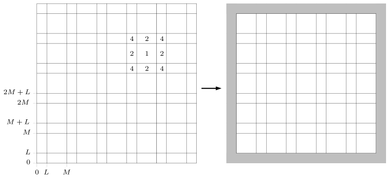
Figure 1. On the left there is the set $\Lambda_{N}$, covered by partially superposed boxes of edge length $M+L$ (the picture is drawn for $d=2$ just for the sake of visualization purpose: $d2$ is not a relevant dimension for our problem ). One of this boxes is highlighted by the numbers $1$, $2$ and $4$: one (and only one) of the fields $\phi^{(z)}$ is supported, for a well chosen $z=z_{\star}\in{\mathbb{Z}}^{d}$, exactly on this box. On the region marked by $1$, of edge length $M-L$, only one field $\phi^{(z)}$ is non zero, that is $\phi^{(z)}(x)=0$ for every $z\neq z_{\star}$ and $x$ in the region marked by $1$. In the regions, belonging to the frame of region $1$, marked by $2$ and $4$, there are respectively $2$ and $4$ values of $z$ (one is $z_{\star}$) for which the $\phi^{(z)}$ fields are non zero. Of course this frame is much smaller than the box ($M\sim L^{2}$). moreover in dimension $d$ there are regions in which up to $2^{d}$ fields superpose. Step 2 in the proof consists in showing that we can erase the contacts in the shadowed frame of the large box $\Lambda_{N}$ at little price: we will see that in the end this fully deals with the boundary effects because the long range correlations of the field are all carried by the field $\phi_{0}$ and we get rid of this field in Step 3.

Now let us show that one can replace $\widetilde{\Lambda}_{N}$ in (3.36) by a smaller set in order to avoid boundary effects. Set

$$\Lambda^{\prime}_{N}=\llbracket L+1,kM\rrbracket^{d}\quad\text{ and }\quad\Gamma_{N}:=\widetilde{\Lambda}_{N}\setminus\Lambda^{\prime}_{N}\,.$$ (3.37)

We are going to prove:

Lemma 3.5.

For $h\geq 0$ we have ${\mathbf{P}}^{0}_{N}\otimes{\mathbf{P}}^{2}_{N}$ a.s.

$${\mathbb{E}}\log{\mathbf{E}}^{1}_{N}\left[e^{\sum_{x\in\widetilde{\Lambda}_{N}}(\beta\omega_{x}-\lambda(\beta)+h)\delta^{u}_{x}}\right]\,\geq\,{\mathbb{E}}\log{\mathbf{E}}^{1}_{N}\left[e^{\sum_{x\in\Lambda^{\prime}_{N}}(\beta\omega_{x}-\lambda(\beta)+h)\delta^{u}_{x}}\right]-\lambda(\beta)|\Gamma_{N}|\,.$$ (3.38)

Since the cardinality of $\Gamma_{N}$ is $O(N^{d-1}L)$, our choice of parameter makes the last term negligible with respect to $N^{d}h^{2+\varepsilon}$, and thus combining (3.36) and (3.38), the inequality (3.21) follows if $\varepsilon<1/\kappa_{d}$ (which we therefore assume) and if we show that

$${\mathbb{E}}{\mathbf{E}}^{0}_{N}\log{\mathbf{E}}^{1}_{N}\left[e^{\sum_{x\in\Lambda^{\prime}_{N}}(\beta\omega_{x}-\lambda(\beta)+h)\delta^{u}_{x}}\right]\,\geq\,N^{d}\left(\chi(\beta)h^{2}-C_{\beta}h^{2+\varepsilon}\right).$$ (3.39)

Note that the expectation w.r.t. to ${\mathbf{P}}^{2}_{N}$ is not displayed because $\phi$ restricted to $\Lambda^{\prime}_{N}$ is completely determined by $\phi_{0}$ and $\left(\phi^{(z)}\right)_{z\in\llbracket 0,k-1\rrbracket^{d}}$.

Proof of Lemma 3.5. We let $\mu^{A}_{N}$ be the probability measure defined by

$$\frac{\mathrm{d}\mu^{A}_{N}}{\mathrm{d}{\mathbf{P}}^{1}_{N}}\left((\phi^{(z)})_{z\in\llbracket 0,k-1\rrbracket}\right)=\frac{e^{\sum_{x\in A}(\beta\omega_{x}-\lambda(\beta)+h)\delta^{u}_{x}}}{{\mathbf{E}}^{1}_{N}\left[e^{\sum_{x\in A}(\beta\omega_{x}-\lambda(\beta)+h)\delta^{u}_{x}}\right]},$$ (3.40)

that is the distribution of $(\phi^{(z)})_{z\in\llbracket 0,k-1\rrbracket}$ when interactions with sites in $A$ are taken into account (this measure depends on the realization of $\phi_{0}$ and possibly also of that of $\phi^{(z)}$ for $z\notin\llbracket 0,k-1\rrbracket$). We have

$$\log{\mathbf{E}}^{1}_{N}\left[e^{\sum_{x\in\widetilde{\Lambda}_{N}}(\beta\omega_{x}-\lambda(\beta)+h)\delta^{u}_{x}}\right]\\ =\log{\mathbf{E}}^{1}_{N}\left[e^{\sum_{x\in\Lambda^{\prime}_{N}}(\beta\omega_{x}-\lambda(\beta)+h)\delta^{u}_{x}}\right]+\log\mu^{\Lambda^{\prime}_{N}}_{N}\left[e^{\sum_{x\in\Gamma_{N}}(\beta\omega_{x}-\lambda(\beta)+h)\delta^{u}_{x}}\right],$$ (3.41)

And thus (3.38) follows by Jensen’s inequality as follows:

$${\mathbb{E}}\log\mu^{\Lambda^{\prime}_{N}}_{N}\left[e^{\sum_{x\in\Gamma_{N}}(\beta\omega_{x}-\lambda(\beta)+h)\delta^{u}_{x}}\right]\,\geq\,{\mathbb{E}}\mu^{\Lambda^{\prime}_{N}}_{N}\left[\sum_{x\in\Gamma_{N}}(\beta\omega_{x}-\lambda(\beta)+h)\delta^{u}_{x}\right]\,\geq\,-\lambda(\beta)|\Gamma_{N}|\,,$$ (3.42)

and in the last step we have used the fact that $\mu^{\Lambda^{\prime}_{N}}_{N}$ does not depend on $\{\omega_{x}\}_{x\in\Gamma_{N}}$ and then we have just used that $\sum_{x\in\Gamma_{N}}\delta^{u}_{x}\leq|\Gamma_{N}|$. The proof of Lemma 3.5 is complete. ∎

Step 3: getting rid of the base field $\phi_{0}$

Our next step is to get rid of the dependence in $\phi_{0}$ in (3.39). We can do this combining two facts. Firstly from (3.8) and our choice of the parameters we know that with an overwhelming large probability $\phi_{0}$ is small everywhere. Secondly, from (3.26), we know that the expectation ${\mathbf{E}}^{1}_{N}[\delta^{u}_{x}]$ for $x\in\delta^{u}_{x}$ is not much affected by small variations of $\phi_{0}$. Let us define the event ${\mathcal{C}}_{N}$ by

$${\mathcal{C}}_{N}\,:=\,\left\{\left|\phi_{0}(x)\right|\,\leq\,L^{-1/3}\text{ for every }x\in\Lambda^{\prime}_{N}\right\}\,.$$ (3.43)

A simple union bound using the estimate on the variance (3.8) yields immediately for $h$ small

$${\mathbf{P}}^{0}_{N}\left({\mathcal{C}}^{\complement}_{N}\right)\,\leq\,\exp\left(-L^{1/4}\right)\,.$$ (3.44)

By applying Jensen’s inequality we have also that for every realization of $\phi_{0}$

$${\mathbb{E}}\log{\mathbf{E}}^{1}_{N}\left[e^{\sum_{x\in\Lambda^{\prime}_{N}}(\beta\omega_{x}-\lambda(\beta)+h)\delta^{u}_{x}}\right]\,\geq\,{\mathbf{E}}^{1}_{N}{\mathbb{E}}\left[{\sum_{x\in\Lambda^{\prime}_{N}}(\beta\omega_{x}-\lambda(\beta)+h)\delta^{u}_{x}}\right]\,\geq\,-|\Lambda^{\prime}_{N}|\lambda(\beta),$$ (3.45)

and therefore

$${\mathbb{E}}{\mathbf{E}}^{0}\log{\mathbf{E}}^{1}_{N}\left[e^{\sum_{x\in\Lambda^{\prime}_{N}}(\beta\omega_{x}-\lambda(\beta)+h)\delta^{u}_{x}}\right]\\ \geq{\mathbb{E}}{\mathbf{E}}^{0}_{N}\left[\log{\mathbf{E}}^{1}_{N}\left[e^{\sum_{x\in\Lambda^{\prime}_{N}}(\beta\omega_{x}-\lambda(\beta)+h)\delta^{u}_{x}}\right]\mathbf{1}_{{\mathcal{C}}_{N}}\right]-\lambda(\beta)N^{d}\,{\mathbf{P}}^{0}_{N}\left({\mathcal{C}}^{\complement}_{N}\right)\,.$$ (3.46)

Now recalling (3.44) and (3.22), this implies that (3.39) follows if one proves that for every $\phi_{0}\in{\mathcal{C}}_{N}$

$${\mathbb{E}}\log{\mathbf{E}}^{1}_{N}\left[e^{\sum_{x\in\Lambda^{\prime}_{N}}(\beta\omega_{x}-\lambda(\beta)+h)\delta^{u}_{x}}\right]\,\geq\,N^{d}\left(\chi(\beta)h^{2}-C_{\beta}h^{2+\varepsilon}\right)\,.$$ (3.47)

Note that expressions like for example the leftmost sides of (3.45)–(3.47) are now random variables: they are measurable with respect to the $\sigma$-field generated by $\phi_{0}$. We are going to see that not averaging over $\phi_{0}$ is typically not a problem, at least as long as $\phi_{0}\in{\mathcal{C}}_{N}$. The key result in this direction says that the contact density is not very much affected by conditioning with respect to $\phi_{0}$, as long as $\phi_{0}\in{\mathcal{C}}_{N}$. It will be repeatedly used in the remainder. Here it is:

Lemma 3.6.

For every $\phi_{0}\in{\mathcal{C}}_{N}$, $x\in\Lambda^{\prime}_{N}$ and $h$ sufficiently small we have

$$\left|{\mathbf{E}}^{1}_{N}[\delta^{u}_{x}]-2\chi(\beta)h\right|\,\leq\,hL^{-1/4}\,.$$ (3.48)

Proof of Lemma 3.6. We introduce the practical notation

$$\phi_{1}(x)\,:=\,\sum_{z\in\llbracket 0,k-1\rrbracket^{d}}\phi^{(z)}(x)\,$$ (3.49)

(note that the summation defining $\phi_{1}(x)$ contains between one and $2^{d}$ non-zero terms), and for $x\in\Lambda^{\prime}_{N}$ we have that

$$\begin{split}{\mathbf{E}}^{1}_{N}\left[\delta^{u}_{x}\right]\,&=\,{\mathbf{P}}^{1}_{N}\left(\phi_{1}(x)\in[u-1-\phi_{0}(x),u+1-\phi_{0}(x)]\right)\\ &=\,{\mathbf{P}}\left(\sqrt{\sigma_{d}^{2}-\mathrm{Var}\left(\phi_{0}(x)\right)}\,{\mathcal{N}}\in{[u-1-\phi_{0}(x),u+1-\phi_{0}(x)]}\right)\,,\end{split}$$ (3.50)

where ${\mathbf{P}}$ in the last line is just the law of ${\mathcal{N}}\sim{\mathcal{N}}(0,1)$, which is of course the only random variable in the expression. Now, for small $h$ and assuming that ${\mathcal{C}}_{N}$ holds, by monotonicity the right-hand side  in (3.50) is maximized when $\phi_{0}(x)=L^{1/3}$ and minimized when $\phi_{0}(x)=-L^{1/3}$. If we set $\widetilde{\sigma}:=\sqrt{\sigma_{d}^{2}-\mathrm{Var}\left(\phi_{0}(x)\right)}$, (3.8) (and the fact that $u$ is asymptotically proportional to $\log L$) implies that for $h$ sufficiently small we have

$$\begin{split}\frac{\sigma_{d}}{\widetilde{\sigma}}[u-1+L^{-1/3},u+1+L^{1/3}]\supset[u-1+2L^{-1/3},u+1],\\ \frac{\sigma_{d}}{\widetilde{\sigma}}[u-1-L^{-1/3},u+1-L^{1/3}]\subset[u-1-L^{-1/3},u+1],\end{split}$$

so that

$${\mathbf{P}}\left(\sigma_{d}\,{\mathcal{N}}\in[u-1+2L^{-1/3},u+1]\right)\,\leq\,{\mathbf{E}}^{1}_{N}\left[\delta^{u}_{x}\right]\,\leq\,{\mathbf{P}}\left(\sigma_{d}\,{\mathcal{N}}\in{[u-1-L^{-1/3},u+1]}\right)\,.$$ (3.51)

Now, using (3.26) we obtain that

$$\left|{\mathbf{E}}^{1}_{N}[\delta^{u}_{x}]-2\chi(\beta)h\right|\,\leq\,h{\mathbf{P}}\left(\sigma_{d}\,{\mathcal{N}}\in{[u-1-L^{-1/3},u-1+2L^{-1/3}]}\right)\,\leq\,Chu_{h}L^{-1/3}\,,$$ (3.52)

with $C=C(\beta,d)$ which can be easily read out from (3.26). The proof of Lemma 3.6 is therefore complete. ∎

Step 4: reducing to estimates on $M$-boxes.

We are now going to state two technical results. The first (Lemma 3.8) is (3.47), but with $\Lambda^{\prime}_{N}$ replaced by the set of vertices $x$ which are in the support of a unique $\phi^{(z)}$

$$\Lambda^{\prime\prime}_{N}:=\left\{x\in\Lambda^{\prime}_{N}\ :\ \exists z,\ \phi_{1}(x)=\phi^{(z)}(x),\ {\mathbf{P}}^{1}_{N}-\text{a.s.}\right\}.$$ (3.53)

Note that our condition $L\ll M$ ensures that $|\Lambda^{\prime\prime}_{N}|\sim|\Lambda^{\prime}_{N}|$. The reason why the quantity with $\Lambda^{\prime\prime}_{N}$ is easier to handle is that by independence of the $\phi^{(z)}$, the partition function can be factorized (and its $\log$ becomes simply a sum). For technical reason, we prove in fact (3.47) with $\Lambda^{\prime\prime}_{N}$ but also with an additional constraint of the fields $\phi^{(z)}$.

The second result (Lemma 3.9) states that the portion of the domain that we leave out, i.e. $\Lambda^{\prime}_{N}\setminus\Lambda^{\prime\prime}_{N}$, gives a negligible contribution, this is where the constraint imposed in the statement of the first result are used.

Both results are needed for our proof, but while the second is of a technical nature, the first contains the key second moment argument on which the proof relies.

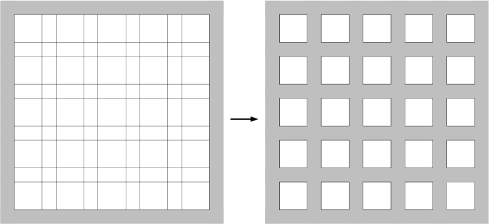
Figure 2. In Step 4 to Step 6 we show that it is sufficient to consider the system in which the contacts in the shadowed grid-like region are erased. The independence properties of the $\phi^{(z)}$ fields reduce the problem to estimate the contributions to the free energy in each of the non shadowed boxes of edge length $M-L$. One important ingredient is also the fact that, for every such a box, we introduce a constraint on the $\phi^{(z)}$ fields whose support intersects the box or its frame (the box with the frame is a box of edgelenth $M+L$). This constraint limits the number of contacts that can take place in this box and its frame. A second moment argument turns out to be very efficient thanks to this control on the number of contacts.

Let us observe that $\Lambda^{\prime\prime}_{N}$ is a disjoint union of cubes of diameter $M-L$

$$\Lambda^{\prime\prime}_{N}\,=\,\bigcup_{z\in\llbracket 0,k-1\rrbracket^{d}}{\mathcal{B}}^{(z)}_{L}\,,$$ (3.54)

where

$${\mathcal{B}}^{(z)}_{L}\,:=\,\llbracket L+1,M\rrbracket^{d}+zM\,.$$ (3.55)

The space between cubes being much smaller than the cube diameter, $\Lambda^{\prime\prime}_{N}$ covers most of the original box. Furthermore let us also introduce

$${\mathcal{D}}_{N}\,:=\,\operatorname*{\bigcap}_{z\in\llbracket 0,k-1\rrbracket^{d}}{\mathcal{D}}^{(z)}_{N}\ \ \textrm{ with }\ \ {\mathcal{D}}^{(z)}_{N}\,:=\,\left\{\phi^{(z)}:\,\left|\left\{x\,:\,\phi^{(z)}(x)\geq 2^{-d}(u-2)\right\}\right|\leq\kappa_{d}\right\}\,.$$ (3.56)

where $\kappa_{d}$ is fixed in such a way that

$$1-{\mathbf{P}}^{1}_{N}\left({\mathcal{D}}^{(z)}_{N}\right)\,=\,{\mathbf{P}}^{1}_{N}\left(\left|\left\{x\ :\ \phi^{(z)}(x)\geq 2^{-d}(u-2)\right\}\right|>\kappa_{d}\right)\,\leq\,h^{2}\,.$$ (3.57)

Note that ${\mathcal{D}}_{N}$ limits the number of contact points. Let us show that we can find $\kappa_{d}$ such that (3.57) holds.

Lemma 3.7.

For any $c>0$ we can find $\kappa=\kappa(d,c)\in{\mathbb{N}}$ such that for $h$ small

$${\mathbf{P}}^{1}_{N}\left(\left|\left\{x\ :\ \phi^{(z)}(x)\geq c\sqrt{2\log(1/h)}\right\}\right|>\kappa\right)\,\leq\,h^{2}\,.$$ (3.58)

Of course (3.57) holds by Lemma 3.7 by choosing a value of $c\in(0,2^{-d}\sigma_{d})$ and then fixing $\kappa_{d}=\max(\kappa(d,c),4d)$ (the requirement $\kappa_{d}\geq 4d$ is due to (3.90) below).

Proof.

By a union bound the probability on the left-hand side of (3.58) is not larger than

$$(M+L)^{d\kappa}\max_{x_{1},\ldots,x_{\kappa}}{\mathbf{P}}^{1}_{N}\left(\phi^{(z)}(x_{j})\geq c\sqrt{2\log(1/h)}\textrm{ for }j=1,\ldots,\kappa\right)\,\leq\\ (2M)^{d\kappa}\max_{x_{1},\ldots,x_{\kappa}}{\mathbf{P}}^{1}_{N}\left(\sum_{j=1}^{\kappa}\phi^{(z)}(x_{j})\geq c\kappa\sqrt{2\log(1/h)}\right)\,,$$ (3.59)

where of course the $x_{j}$’s are in the support of $\phi^{(z)}$. We are therefore reduced to estimating the variance of $\sum_{j=1}^{\kappa}\phi^{(z)}(x_{j})$. The first observation is that we can replace ${\mathbf{P}}^{1}_{N}$ with ${\mathbf{P}}$, that is we can work with the free field in ${\mathbb{Z}}^{d}$ (this is just because $G(x,y)$ is larger than the covariance of $\phi^{(z)}$ for every choice of $x$ and $y$). The next step is realizing that this variance is maximal when the $x_{j}$ are closely packed: more precisely that the maximum of the variance is bounded above by a constant that depends only on the dimension time the variance of the case in which the set $\{x_{1},\ldots,x_{\kappa}\}$ is replaced by the cube of edge length equal to $\lceil\kappa^{1/d}\rceil$ (of course this cube contains more than $\kappa$ points, unless $\kappa^{1/d}$ is an integer number: the full argument is left to the reader and can be found for example in [21, Lemma 6.11] where one can refer also for an explicit constant (that is however largely overestimated). The computation for the cube is straightforward and yields a variance which behaves for $\kappa$ large like $C_{d}\kappa^{(d+2)/d}$. Therefore

$$\begin{split}{\mathbf{P}}^{1}_{N}\left(\sum_{j=1}^{\kappa}\phi^{(z)}(x_{j})\geq c\kappa\sqrt{2\log(1/h)}\right)\,&\leq\,{\mathbf{P}}\left(\sigma_{d}{\mathcal{N}}\,\geq\,c\,C_{d}^{-1/2}\kappa^{1-(d+2)/(2d)}\sqrt{2\log(1/h)}\right)\\ &\leq\,h^{c^{2}\kappa^{(d-2)/d}/(C_{d}\sigma_{d}^{2})}\,=\,h^{c^{\prime}_{d}\kappa^{(d-2)/d}}\,.\end{split}$$ (3.60)

Therefore

$${\mathbf{P}}^{1}_{N}\left(\left|\left\{x\ :\ \phi^{(z)}(x)\geq 2^{-d}(u-2)\right\}\right|>\kappa\right)\,\leq\,2^{d\kappa}h^{-2d+c^{\prime}_{d}\kappa^{(d-2)/d}}\,\leq\,h^{2}\,,$$ (3.61)

with the last step that holds if $\kappa$ is chosen so that $c^{\prime}_{d}\kappa^{(d-2)/d}>2d+2$ and if $h$ is sufficiently small. Therefore $\kappa(d,c)$ is identified and the proof of Lemma 3.7 is complete. ∎

Here is the first of the two results that we announced:

Lemma 3.8.

For every $\phi_{0}\in{\mathcal{C}}_{N}$ we have (note that $|{\mathcal{B}}^{(z)}_{L}|=(M-L)^{d}=L^{2d}$)

$${\mathbb{E}}\log{\mathbf{E}}^{1}_{N}\left[e^{\sum_{x\in{\mathcal{B}}_{L}^{(z)}}(\beta\omega_{x}-\lambda(\beta)+h)\delta^{u}_{x}}\mathbf{1}_{{\mathcal{D}}^{(z)}_{N}}\right]\,\geq\,L^{2d}(\chi(\beta)h^{2}-C_{\beta}h^{2+\varepsilon}).$$ (3.62)

As a consequence for $\phi_{0}\in{\mathcal{C}}_{N}$ we have

$$\begin{split}{\mathbb{E}}\log{\mathbf{E}}^{1}_{N}\left[e^{\sum_{x\in\Lambda^{\prime\prime}_{N}}(\beta\omega_{x}-\lambda(\beta)+h)\delta^{u}_{x}}\mathbf{1}_{{\mathcal{D}}_{N}}\right]\,&=\sum_{z\in\llbracket 0,k-1\rrbracket^{d}}{\mathbb{E}}\log{\mathbf{E}}^{1}_{N}\left[e^{\sum_{x\in{\mathcal{B}}_{L}^{(z)}}(\beta\omega_{x}-\lambda(\beta)+h)\delta^{u}_{x}}\mathbf{1}_{{\mathcal{D}}^{(z)}_{N}}\right]\\ &\geq\,N^{d}(\chi(\beta)h^{2}-C_{\beta}h^{2+\varepsilon})\,.\end{split}$$ (3.63)

Of course this is not yet sufficient to conclude as there is no direct way to show that adding the sites of $\Lambda^{\prime}_{N}\setminus\Lambda^{\prime\prime}_{N}$ has a positive contribution on the free energy.

We will in fact content ourselves with showing that this contribution is not too negative. This is the object of our second result. It requires the introduction of some further notation. We define for $A\subset\Lambda^{\prime}_{N}$, $\widetilde{Z}_{A,\omega}$ as a partition function restricted to ${\mathcal{D}}_{N}$ for which the interaction is present only for sites in $A$

$$\widetilde{Z}_{A,\omega}\,:=\,{\mathbf{E}}^{1}_{N}\left[e^{\sum_{x\in A}(\beta\omega_{x}-\lambda(\beta)+h)\delta^{u}_{x}}\mathbf{1}_{{\mathcal{D}}_{N}}\right]\,.$$ (3.64)

Moreover we define

$$K_{h}\,:=\,\inf\{K\geq\sqrt{\log 1/h}:\,{\mathbb{E}}[|\omega_{x}|\,;\,|\omega_{x}|>K]\leq h^{3}\}\,.$$ (3.65)

The condition $K\geq\sqrt{\log 1/h}$ is artificial, but it is convenient for us to have $\lim_{h\searrow 0}K_{h}=\infty$. Since we have assumed ${\mathbb{E}}[\exp(t\omega_{x})]<\infty$ for every $t\in{\mathbb{R}}$ we have that $K_{h}=o(\log(1/h))$. We set

$$\mkern 1.5mu\overline{\mkern-1.5mu\omega\mkern-1.5mu}\mkern 1.5mu_{x}\,:=\,\omega_{x}\mathbf{1}_{\{|\omega_{x}|\leq K_{h}\}}.$$ (3.66)

Here is the second result.

Lemma 3.9.

For every $\gamma>0$ there exists $h_{0}$ such that for all $h\in[0,h_{0}]$ we have

$${\mathbb{E}}\log\widetilde{Z}_{B,\mkern 1.5mu\overline{\mkern-1.5mu\omega\mkern-1.5mu}\mkern 1.5mu}-{\mathbb{E}}\log\widetilde{Z}_{A,\mkern 1.5mu\overline{\mkern-1.5mu\omega\mkern-1.5mu}\mkern 1.5mu}\,\geq\,-h^{2-\gamma}\left|B\setminus A\right|\,,$$ (3.67)

for every $A$ and $B$ with $A\subset B\subset\Lambda^{\prime}_{N}$

Let us show that combining Lemma 3.8 and Lemma 3.9 we obtain (3.47) (and the proof of Proposition 3.1 is therefore reduced to proving the two lemmas). First of all just by restricting the expectation to the event ${\mathcal{D}}_{N}$ we have

$${\mathbb{E}}\log{\mathbf{E}}^{1}_{N}\left[e^{\sum_{x\in\Lambda^{\prime}_{N}}(\beta\omega_{x}-\lambda(\beta)+h)\delta^{u}_{x}}\right]\,\geq{\mathbb{E}}\log{\mathbf{E}}^{1}_{N}\left[e^{\sum_{x\in\Lambda^{\prime}_{N}}(\beta\omega_{x}-\lambda(\beta)+h)\delta^{u}_{x}}\mathbf{1}_{{\mathcal{D}}_{N}}\right]$$ (3.68)

The next step is to remark that we can replace $\omega_{x}$ by $\mkern 1.5mu\overline{\mkern-1.5mu\omega\mkern-1.5mu}\mkern 1.5mu_{x}$ without changing much the expectation. In fact, by applying Lemma A.3 with $K=K_{h}$ we see that for any $A\subset\Lambda^{\prime}_{N}$ we have

$$\left|{\mathbb{E}}\left[\log\widetilde{Z}_{A,\omega}\right]-{\mathbb{E}}\left[\log\widetilde{Z}_{A,\mkern 1.5mu\overline{\mkern-1.5mu\omega\mkern-1.5mu}\mkern 1.5mu}\right]\right|\leq\beta|A|h^{3}.$$ (3.69)

In particular, using (3.69) for $A=\Lambda^{\prime}_{N}$ we see that it is sufficient to prove (3.47) for

$${\mathbb{E}}\left[\log\widetilde{Z}_{\Lambda^{\prime}_{N},\mkern 1.5mu\overline{\mkern-1.5mu\omega\mkern-1.5mu}\mkern 1.5mu}\right]={\mathbb{E}}\left[\log\widetilde{Z}_{\Lambda^{\prime\prime}_{N},\mkern 1.5mu\overline{\mkern-1.5mu\omega\mkern-1.5mu}\mkern 1.5mu}\right]+{\mathbb{E}}\left[\log\widetilde{Z}_{\Lambda^{\prime}_{N},\mkern 1.5mu\overline{\mkern-1.5mu\omega\mkern-1.5mu}\mkern 1.5mu}-\log\widetilde{Z}_{\Lambda^{\prime\prime}_{N},\mkern 1.5mu\overline{\mkern-1.5mu\omega\mkern-1.5mu}\mkern 1.5mu}\right]$$ (3.70)

We now use Lemma 3.8 and (3.69) to bound the first term and Lemma 3.9 for the second one and we obtain that for $\gamma>0$ and $h$ sufficiently small (allowed to depend on $\gamma$)

$${\mathbb{E}}\log{\mathbf{E}}^{1}_{N}\left[e^{\sum_{x\in\Lambda^{\prime}_{N}}(\beta\omega_{x}-\lambda(\beta)+h)\delta^{u}_{x}}\right]\geq\,N^{d}(\chi(\beta)h^{2}-C_{\beta}h^{2+\varepsilon})-|\Lambda^{\prime}_{N}\setminus\Lambda^{\prime\prime}_{N}|h^{2-\gamma}\,.$$ (3.71)

Now it suffices to recall the choice of the parameters and to choose $\gamma=1/2\kappa_{d}$ and (3.22) allows to conclude that (3.47) holds for some $\varepsilon>0$. More precisely we have

$$|\Lambda^{\prime}_{N}\setminus\Lambda^{\prime\prime}_{N}|\leq d(k+1)LN^{d-1}\leq 2dN^{d}L^{-1}=2dN^{d}h^{\frac{1}{\kappa}_{d}}.$$ (3.72)

As announced, this means that we are just left with proving Lemma 3.8 and Lemma 3.9. This is the content of the next two steps of the proof.

Step 5: the second moment estimate (proof of Lemma 3.8)

To see that (3.63) follows from (3.62), one simply observes that once $\phi_{0}$ is fixed, $(\delta^{u}_{x})_{x\in{\mathcal{B}}_{L}^{(z)}}$ is determined by $\phi^{(z)}$. Hence, since ${\mathbf{P}}^{1}_{N}$ is a product measure (recall the support properties of $\phi^{(z)}$ and the definition (3.55) of ${\mathcal{B}}^{(z)}_{L}$), the expectation can be factorized. Applying (3.62) to each term of the sum thus obtained we have

$${\mathbb{E}}\log{\mathbf{E}}^{1}_{N}\left[e^{\sum_{x\in\Lambda^{\prime}_{N}}(\beta\omega_{x}-\lambda(\beta)+h)\delta^{u}_{x}}\right]\geq|\Lambda^{\prime\prime}_{N}|(\chi(\beta)h^{2}-C_{\beta}h^{2+\varepsilon}),$$

and we conclude (modifying the value of $C_{\beta}$ if necessary) by using the fact that our choice of parameters implies $|\Lambda^{\prime\prime}_{N}|\geq N^{d}(1-h^{\varepsilon})$.

Let us now turn to the important part which is the proof of (3.62). Since the result does not depend on $z$ let us assume that $z=0$ and write ${\mathcal{B}}$ for ${\mathcal{B}}^{(z)}_{L}$. With this notational simplification we remark the splitting:

$${\mathbb{E}}\log{\mathbf{E}}^{1}_{N}\left[e^{\sum_{x\in{\mathcal{B}}}(\beta\omega_{x}-\lambda(\beta)+h)\delta^{u}_{x}}\mathbf{1}_{{\mathcal{D}}^{(0)}_{N}}\right]\,=\\ {\mathbb{E}}\log\frac{{\mathbf{E}}^{1}_{N}\left[e^{\sum_{x\in{\mathcal{B}}}(\beta\omega_{x}-\lambda(\beta)+h)\delta^{u}_{x}}\mathbf{1}_{{\mathcal{D}}^{(0)}_{N}}\right]}{{\mathbb{E}}{\mathbf{E}}^{1}_{N}\left[e^{\sum_{x\in{\mathcal{B}}}(\beta\omega_{x}-\lambda(\beta)+h)\delta^{u}_{x}}\mathbf{1}_{{\mathcal{D}}^{(0)}_{N}}\right]}+\log{\mathbb{E}}{\mathbf{E}}^{1}_{N}\left[e^{\sum_{x\in{\mathcal{B}}}(\beta\omega_{x}-\lambda(\beta)+h)\delta^{u}_{x}}\mathbf{1}_{{\mathcal{D}}^{(0)}_{N}}\right]\\ =\,{\mathbb{E}}\log{\mathbf{E}}^{1,h}_{N}\left[e^{\sum_{x\in{\mathcal{B}}}(\beta\omega_{x}-\lambda(\beta))\delta^{u}_{x}}\,\Big{|}\,{{\mathcal{D}}^{(0)}_{N}}\right]+\log{\mathbb{E}}{\mathbf{E}}^{1}_{N}\left[e^{h\sum_{x\in{\mathcal{B}}}\delta^{u}_{x}}\mathbf{1}_{{\mathcal{D}}^{(0)}_{N}}\right]\,,$$ (3.73)

and in the last step we have introduced the homogeneous pinning Gibbs measure ${\mathbf{P}}^{1,h}_{N}$. Let us first estimate the last addendum in (3.73). We have

$$\begin{split}\log{\mathbf{E}}^{1}_{N}\left[e^{\sum_{x\in{\mathcal{B}}}h\delta^{u}_{x}}\mathbf{1}_{{\mathcal{D}}^{({0})}_{N}}\right]\,&\geq\,h\,{\mathbf{E}}^{1}_{N}\left[\sum_{x\in{\mathcal{B}}}\delta^{u}_{x}\,\bigg{|}\,{\mathcal{D}}^{({0})}_{N}\right]+\log{\mathbf{P}}^{1}_{N}({\mathcal{D}}^{({0})}_{N})\\ &\geq\,h\,{\mathbf{E}}^{1}_{N}\left[\left(\sum_{x\in{\mathcal{B}}}\delta^{u}_{x}\right)\mathbf{1}_{{\mathcal{D}}^{({0})}_{N}}\right]+\log{\mathbf{P}}^{1}_{N}({\mathcal{D}}^{({0})}_{N})\\ &=\,h\,{\mathbf{E}}^{1}_{N}\left[\sum_{x\in{\mathcal{B}}}\delta^{u}_{x}\right]-h{\mathbf{E}}^{1}_{N}\left[\left(\sum_{x\in{\mathcal{B}}}\delta^{u}_{x}\right)\mathbf{1}_{\left({\mathcal{D}}^{({0})}_{N}\right)^{\complement}}\right]+\log{\mathbf{P}}^{1}_{N}({\mathcal{D}}^{({0})}_{N})\\ &\geq\,L^{2d}\left(2\chi(\beta)h^{2}+O\left(h^{2}L^{-1/4}\right)\right)-L^{2d}h^{3}-2h^{2}\\ &\geq\,L^{2d}\left(2\chi(\beta)h^{2}-C_{\beta}h^{2+\varepsilon}\right)\,,\end{split}$$ (3.74)

where in the step before the last one the three terms correspond to the three terms in the previous line and we have used, in order, (3.48), then (3.57) together with $\sum_{x\in{\mathcal{B}}}\delta^{u}_{x}\leq L^{2d}$ and finally again (3.57).

We are left with estimating first addendum in (3.73). Note that since ${\mathbf{P}}^{1,h}_{N}(\cdot\ |\,{\mathcal{D}}^{({0})}_{N})$ is a small modification of ${\mathbf{P}}^{1}_{N}$, the probability of making one contact in ${\mathcal{B}}$ is small also under the former measure. In fact

$$\begin{split}{\mathbf{P}}^{1,h}_{N}\left(\sum_{x\in{\mathcal{B}}}\delta^{u}_{x}\,\geq\,1\,\bigg{|}\,{\mathcal{D}}^{({0})}_{N}\right)\,&=\,\frac{{\mathbf{E}}^{1}_{N}\left[e^{h\sum_{x\in{\mathcal{B}}}\delta^{u}_{x}}\mathbf{1}_{\left\{\sum_{x\in{\mathcal{B}}}\delta^{u}_{x}\,\geq\,1\right\}\cap{\mathcal{D}}^{(0)}_{N}}\right]}{{\mathbf{E}}^{1}_{N}\left[e^{h\sum_{x\in{\mathcal{B}}}\delta^{u}_{x}}\mathbf{1}_{{\mathcal{D}}^{(0)}_{N}}\right]}\\ &\leq\,\frac{e^{h\kappa_{d}}{\mathbf{P}}^{1}_{N}\left({\left\{\sum_{x\in{\mathcal{B}}}\delta^{u}_{x}\,\geq\,1\right\}\cap{\mathcal{D}}^{(0)}_{N}}\right)}{{\mathbf{P}}^{1}_{N}\left({{\mathcal{D}}^{(0)}_{N}}\right)}\\ &\leq\,(1+2\kappa_{d}h){\mathbf{P}}^{1}_{N}\left({\left\{\sum_{x\in{\mathcal{B}}}\delta^{u}_{x}\,\geq\,1\right\}\cap{\mathcal{D}}^{(0)}_{N}}\right)\\ &\leq\,(1+2\kappa_{d}h){\mathbf{P}}^{1}_{N}\left(\sum_{x\in{\mathcal{B}}}\delta^{u}_{x}\,\geq\,1\right)\\ &\leq\,(1+2\kappa_{d}h)\sum_{x\in{\mathcal{B}}}{\mathbf{E}}^{1}_{N}\left[\delta^{u}_{x}\right]\,\leq\,C_{1}(\beta)L^{2d}h\,,\end{split}$$ (3.75)

where in the second inequality we used (3.57) and in the last one we have used (3.48) and $C_{1}(\beta):=4\chi(\beta)$. As a consequence we have for every $\omega$

$${\mathbf{E}}^{1,h}_{N}\left[e^{\sum_{x\in{\mathcal{B}}}(\beta\omega_{x}-\lambda(\beta))\delta^{u}_{x}}\,\bigg{|}\,{\mathcal{D}}^{({0})}_{N}\right]\,\geq\,1-C_{1}(\beta)L^{2d}h\,.$$ (3.76)

Hence using the formula $\log(1+y)\geq y-\frac{1}{2(1-\eta)}y^{2}$, valid for all $y\geq-\eta$ and $\eta\in(0,1)$, with $\eta=C_{1}(\beta)L^{2d}h$ we obtain that

$${\mathbb{E}}\log{\mathbf{E}}^{1,h}_{N}\left[e^{\sum_{x\in{\mathcal{B}}}(\beta\omega_{x}-\lambda(\beta))\delta^{u}_{x}}\,\Big{|}\,{\mathcal{D}}^{({0})}_{N}\right]\\ \geq\,-\frac{1}{2(1-C_{1}(\beta)L^{2d}h)}\left({\mathbb{E}}\left({\mathbf{E}}^{1}_{N}\left[e^{\sum_{x\in{\mathcal{B}}}(\beta\omega_{x}-\lambda(\beta))\delta^{u}_{x}}\,\Big{|}\,{\mathcal{D}}^{({0})}_{N}\right]^{2}\right)-1\right)\\ \geq\,-\frac{1}{2}\left(1+2C_{1}(\beta)L^{2d}h\right)\left(\left(\widetilde{\mathbf{E}}^{1}_{N}\right)^{\otimes 2}\left[e^{\sum_{x\in{\mathcal{B}}}(\lambda(2\beta)-2\lambda(\beta))\delta^{(1)}_{x}\delta^{(2)}_{x}}\right]-1\right)\,,$$ (3.77)

where the last inequality it is simply the fact that $1+2x\geq 1/(1-x)$ pour $x\in[0,1/2]$, so we are assuming $C_{1}(\beta)L^{2d}h\leq 1/2$, and we have introduced the notation

$$\widetilde{\mathbf{P}}^{1}_{N}(\cdot)\,:=\,{\mathbf{P}}^{1}_{N}\left(\cdot\,\Big{|}{\mathcal{D}}^{({0})}_{N}\right)\,.$$ (3.78)

The notation $\delta^{(i)}_{x}$, $i=1,2$ denote the set of contact point for the two marginals $\phi^{(i)}$, $i=1,2$ of the product measure $\left(\widetilde{\mathbf{P}}^{1}_{N}\right)^{\otimes 2}$. Now taking advantage of the fact that, because of the restriction to ${\mathcal{D}}^{(0)}_{N}$, under $\left(\widetilde{\mathbf{P}}^{1}_{N}\right)^{\otimes 2}$ we have $\sum_{x\in{\mathcal{B}}}\delta^{(1)}_{x}\delta^{(2)}_{x}\leq\kappa_{d}$, we deduce that

$$\left(\widetilde{\mathbf{E}}^{1}_{N}\right)^{\otimes 2}\left[e^{\sum_{x\in{\mathcal{B}}}(\lambda(2\beta)-2\lambda(\beta))\delta^{(1)}_{x}\delta^{(2)}_{x}}\right]\,\leq\,1-\left(\widetilde{\mathbf{P}}^{1}_{N}\right)^{\otimes 2}\left(\sum_{x\in{\mathcal{B}}}\delta^{(1)}_{x}\delta^{(2)}_{x}\geq 1\right)+\\ e^{\lambda(2\beta)-2\lambda(\beta)}\left(\widetilde{\mathbf{P}}^{1}_{N}\right)^{\otimes 2}\left(\sum_{x\in{\mathcal{B}}}\delta^{(1)}_{x}\delta^{(2)}_{x}=1\right)+e^{\kappa_{d}(\lambda(2\beta)-2\lambda(\beta))}\left(\widetilde{\mathbf{P}}^{1}_{N}\right)^{\otimes 2}\left(\sum_{x\in{\mathcal{B}}}\delta^{(1)}_{x}\delta^{(2)}_{x}\geq 2\right)\\ =\,1+\left(e^{\lambda(2\beta)-2\lambda(\beta)}-1\right)\left(\widetilde{\mathbf{P}}^{1}_{N}\right)^{\otimes 2}\left(\sum_{x\in{\mathcal{B}}}\delta^{(1)}_{x}\delta^{(2)}_{x}=1\right)\\ +\left(e^{\kappa_{d}(\lambda(2\beta)-2\lambda(\beta))}-1\right)\left(\widetilde{\mathbf{P}}^{1}_{N}\right)^{\otimes 2}\left(\sum_{x\in{\mathcal{B}}}\delta^{(1)}_{x}\delta^{(2)}_{x}\geq 2\right).$$ (3.79)

In the following lemma (whose proof we postpone), we compute a sharp upper bound for the second term in the sum, and show that the third one is negligible.

Lemma 3.10.

Set $\varepsilon=1/(4\kappa_{d})$. There exists $h_{0}=h_{0}(\beta,d)$ such that for $h\in(0,h_{0}(\beta,d))$ and $\phi_{0}\in{\mathcal{C}}_{N}$ we have

$$\left(\widetilde{\mathbf{E}}^{1}_{N}\right)^{\otimes 2}\left(\sum_{x\in{\mathcal{B}}}\delta^{(1)}_{x}\delta^{(2)}_{x}\right)\,\leq\,\left((2\chi(\beta)h)^{2}+h^{2+\varepsilon}\right)L^{2d}\,,$$ (3.80)

and

$$\left(\widetilde{\mathbf{P}}^{1}_{N}\right)^{\otimes 2}\left(\sum_{x\in{\mathcal{B}}}\delta^{(1)}_{x}\delta^{(2)}_{x}\geq 2\right)\,\leq\,h^{2+\varepsilon}L^{2d}\,.$$ (3.81)

The application of Lemma 3.10 to (3.79) yields (for adequate choice of constants)

$$\left(\widetilde{\mathbf{E}}^{1}_{N}\right)^{\otimes 2}\left[e^{\sum_{x\in{\mathcal{B}}}(\lambda(2\beta)-2\lambda(\beta))\delta^{(1)}_{x}\delta^{(2)}_{x}}\right]-1\,\geq\\ \frac{1}{2\chi(\beta)}\left((2\chi(\beta)h)^{2}+Ch^{2+\varepsilon}\right)L^{2d}-Ch^{2+\varepsilon}\left(e^{\kappa_{d}(\lambda(2\beta)-2\lambda(\beta))}-1\right)L^{2d}\\ =\,\left(2\chi(\beta)h^{2}-C^{\prime}h^{2+\varepsilon}\right)L^{2d}\,,$$ (3.82)

and going back to (3.77) we get (for a different constant $C$)

$${\mathbb{E}}\log{\mathbf{E}}^{1,h}_{N}\left[e^{\sum_{x\in{\mathcal{B}}}(\beta\omega_{x}-\lambda(\beta))\delta^{u}_{x}}\,\Big{|}\,{\mathcal{D}}^{({0})}_{N}\right]\,\geq\,\left(\chi(\beta)h^{2}-Ch^{2+\varepsilon}\right)L^{2d}\,,$$ (3.83)

and we are done with the proof of Lemma 3.8. ∎

Proof of Lemma 3.10. The proof relies essentially on controlling the first and second moment of the sum $\sum_{x\in{\mathcal{B}}}\delta^{(1)}_{x}\delta^{(2)}_{x}$. For what concerns (3.80) we observe that

$$\left(\widetilde{\mathbf{E}}^{1}_{N}\right)^{\otimes 2}\left(\sum_{x\in{\mathcal{B}}}\delta^{(1)}_{x}\delta^{(2)}_{x}\right)\,=\,\sum_{x\in{\mathcal{B}}}\left(\widetilde{\mathbf{E}}^{1}_{N}\left[\delta^{u}_{x}\right]\right)^{2}\,,$$ (3.84)

and that

$$\begin{split}\widetilde{\mathbf{E}}^{1}_{N}\left[\delta^{u}_{x}\right]\,=\,\frac{{\mathbf{E}}^{1}_{N}\left[\delta^{u}_{x}\mathbf{1}_{{\mathcal{D}}_{N}^{(0)}}\right]}{{\mathbf{P}}^{1}_{N}\left({\mathcal{D}}_{N}^{(0)}\right)}\,\leq\,(1+2h^{2}){\mathbf{E}}^{1}_{N}\left[\delta^{u}_{x}\right]\,&\leq\,(1+2h^{2})\left(2\chi(\beta)h+hL^{-1/4}\right)\\ &\leq\,2\chi(\beta)h+h^{1+b}\,,\end{split}$$ (3.85)

and in the last step $b$ is any positive number smaller than $1/(4\kappa_{d})$ and the step holds for $h$ smaller that a constant that depends on $\beta$, $d$ and on the choice of $b$. Therefore the square of this last expression is bounded by $(2\chi(\beta)h)^{2}+h^{2+b}$, for example $b=1/(5\kappa_{d})$ for $h$ smaller than a constant that depends only on $\beta$ and $d$. The proof of (3.80) is therefore complete.

For what concerns (3.81) we start like for (3.80), that is we get rid of the conditioning with respect to ${\mathcal{D}}_{N}^{(0)}$ and then we proceed with a union bound:

$$\begin{split}\left(\widetilde{\mathbf{P}}^{1}_{N}\right)^{\otimes 2}\left(\sum_{x\in{\mathcal{B}}}\delta^{(1)}_{x}\delta^{(2)}_{x}\geq 2\right)\,&\leq\,(1+2h^{2})^{2}\left({\mathbf{P}}^{1}_{N}\right)^{\otimes 2}\left(\sum_{x\in{\mathcal{B}}}\delta^{(1)}_{x}\delta^{(2)}_{x}\geq 2\right)\\ \,&\leq\,(1+2h^{2})^{2}\sum_{x,y\in{\mathcal{B}}:\,x\neq y}\left({\mathbf{P}}^{1}_{N}\right)^{\otimes 2}\left(\delta^{(1)}_{x}\delta^{(2)}_{x}\delta^{(1)}_{y}\delta^{(2)}_{y}=1\right)\\ \,&=\,(1+2h^{2})^{2}\sum_{x,y\in{\mathcal{B}}:\,x\neq y}{\mathbf{P}}^{1}_{N}\left(\delta^{u}_{x}\delta^{u}_{y}=1\right)^{2}\\ \,&\leq\,(1+2h^{2})^{2}L^{4d}\max_{x\neq y}{\mathbf{P}}^{1}_{N}\left(\delta^{u}_{x}\delta^{u}_{y}=1\right)^{2}\,.\end{split}$$ (3.86)

We proceed by observing that (recall (3.49))

$$\begin{split}{\mathbf{P}}^{1}_{N}\left(\delta^{u}_{x}\delta^{u}_{y}=1\right)\,&\leq\,{\mathbf{P}}^{1}_{N}\left(\phi_{1}(x)\geq u-1-\phi_{0}(x),\,\phi_{1}(y)\geq u-1-\phi_{0}(x)\right)\\ &\leq\,{\mathbf{P}}^{1}_{N}\left(\phi_{1}(x)+\phi_{1}(y)\geq 2u-3\right)\,.\end{split}$$ (3.87)

This is just a Gaussian tail estimate for a centered Gaussian variable with variance equal to $\mathrm{Var}(\phi(x)+\phi(y)-\phi_{0}(x)-\phi_{0}(y))=\mathrm{Var}(\phi(x)+\phi(y))-\mathrm{Var}(\phi_{0}(x)+\phi_{0}(y))$ and, for $x\neq 0$, it is therefore smaller than $\mathrm{Var}(\phi(x)+\phi(y)=2(1+p(d))\sigma^{2}_{d}$, where $p(d)\in(0,1)$ is the probability that the the simple random walk, starting from the origin, revisits the origin. The constant $p(d)$ has an expression in terms of an integral involving a Bessel function (see for example [14, Section 5.9]), in particular $p(d)$ decreases to zero as $d$ becomes large: here we will just use $p(d)\leq p(3)=0.3405\ldots<7/20$). Hence we are left with estimating

$${\mathbf{P}}^{1}_{N}\left(\delta^{u}_{x}\delta^{u}_{y}=1\right)\,\leq\,{\mathbf{P}}\left(\sqrt{2(1+p(d))}\sigma_{d}{\mathcal{N}}\,\geq\,2u-3\right)\,,$$ (3.88)

and (3.28), along with the fact that $u_{h}$ is asymptotically equivalent to $\sigma_{d}\sqrt{2\log(1/h)}$, readily yields that

$${\mathbf{P}}^{1}_{N}\left(\delta^{u}_{x}\delta^{u}_{y}=1\right)\,\leq\,h^{1+b}\,,$$ (3.89)

for every $b\in(0,(1-p(d))/(1+p(d)))$, and $h$ sufficiently small. Going back to (3.86)we conclude that

$$\left(\widetilde{\mathbf{P}}^{1}_{N}\right)^{\otimes 2}\left(\sum_{x\in{\mathcal{B}}}\delta^{(1)}_{x}\delta^{(2)}_{x}\geq 2\right)\,\leq\,L^{4d}h^{2+2b}\,=\,L^{2d}h^{2+2b-2d/\kappa_{d}}\,,$$ (3.90)

for every $b\in(0,(1-p(d))/(1+p(d)))$ and $h$ sufficiently small. Since $(1-x)/(1+x)>(1-2x)$ for every $x>0$ we can choose $b=1-2p(d)>1-7/10=3/10$. Since $2b-2d/\kappa_{d}>3/5-2d/\kappa_{d}\geq 1/10>1/(4\kappa_{d})$ (for the last inequality and the one before the last one, recall that $\kappa_{d}$ is chosen to be at least $4d$) and this completes the proof of Lemma 3.10. ∎

Step 6: the proof of Lemma 3.9

Of course it is sufficient to prove the result for $B=A\cup\{x\}$, because then the general results can be obtained by adding vertices one by one. We just have to prove then that

$${\mathbb{E}}\log\widetilde{\nu}^{A,\mkern 1.5mu\overline{\mkern-1.5mu\omega\mkern-1.5mu}\mkern 1.5mu}\left(e^{(\beta\mkern 1.5mu\overline{\mkern-1.5mu\omega\mkern-1.5mu}\mkern 1.5mu_{x}-\lambda(\beta)+h)\delta^{u}_{x}}\right)\geq-Ch^{2-\gamma}.$$ (3.91)

where $\widetilde{\nu}^{A,\mkern 1.5mu\overline{\mkern-1.5mu\omega\mkern-1.5mu}\mkern 1.5mu}$ denotes to the distribution of $(\phi^{(z)})_{z\in{\mathbb{Z}}^{d}}$ associated with the partition function $\widetilde{Z}_{A,\mkern 1.5mu\overline{\mkern-1.5mu\omega\mkern-1.5mu}\mkern 1.5mu}$, cf. (3.64): note that it depends only on $(\mkern 1.5mu\overline{\mkern-1.5mu\omega\mkern-1.5mu}\mkern 1.5mu_{y})_{y\in A}$. We are going to show a stronger statement than (3.91): in fact we are going to show that (3.91) holds also if we average only with respect to $\mkern 1.5mu\overline{\mkern-1.5mu\omega\mkern-1.5mu}\mkern 1.5mu_{x}$ (we use the notation ${\mathbb{E}}_{x}$) and we freeze the realization of $(\mkern 1.5mu\overline{\mkern-1.5mu\omega\mkern-1.5mu}\mkern 1.5mu_{y})_{y\neq x}$. Setting $p_{A,\mkern 1.5mu\overline{\mkern-1.5mu\omega\mkern-1.5mu}\mkern 1.5mu}=p_{A,\mkern 1.5mu\overline{\mkern-1.5mu\omega\mkern-1.5mu}\mkern 1.5mu,\beta,h}:=\widetilde{\nu}^{A,\mkern 1.5mu\overline{\mkern-1.5mu\omega\mkern-1.5mu}\mkern 1.5mu}(\delta^{u}_{x}=1)$ – it is a random variable measurable with respect to $(\mkern 1.5mu\overline{\mkern-1.5mu\omega\mkern-1.5mu}\mkern 1.5mu_{y})_{y\in A}$ – we have

$$\begin{split}{\mathbb{E}}_{x}\log\widetilde{\nu}^{A,\mkern 1.5mu\overline{\mkern-1.5mu\omega\mkern-1.5mu}\mkern 1.5mu}\left[e^{(\beta\mkern 1.5mu\overline{\mkern-1.5mu\omega\mkern-1.5mu}\mkern 1.5mu_{x}-\lambda(\beta)+h)\delta^{u}_{x}}\right]\,&=\,{\mathbb{E}}_{x}\log\left(1+p_{A,\mkern 1.5mu\overline{\mkern-1.5mu\omega\mkern-1.5mu}\mkern 1.5mu}\left(e^{\beta\mkern 1.5mu\overline{\mkern-1.5mu\omega\mkern-1.5mu}\mkern 1.5mu_{x}-\lambda(\beta)+h}-1\right)\right)\,\\ &\geq\,-p_{A,\mkern 1.5mu\overline{\mkern-1.5mu\omega\mkern-1.5mu}\mkern 1.5mu}^{2}\left(e^{\lambda(2\beta)-2\lambda(\beta)}-1\right)\,,\end{split}$$ (3.92)

where in the last step holds if $p_{A,\mkern 1.5mu\overline{\mkern-1.5mu\omega\mkern-1.5mu}\mkern 1.5mu}\leq 1/2$, so we can use the inequality $\log(1+y)\geq y-y^{2}$ that holds for $y\geq-1/2$: in fact $p_{A,\mkern 1.5mu\overline{\mkern-1.5mu\omega\mkern-1.5mu}\mkern 1.5mu}\leq 1/2$ yields $p_{A,\mkern 1.5mu\overline{\mkern-1.5mu\omega\mkern-1.5mu}\mkern 1.5mu}(e^{\beta\mkern 1.5mu\overline{\mkern-1.5mu\omega\mkern-1.5mu}\mkern 1.5mu-\lambda(\beta)}-1)\geq-1/2$ for every value of $\mkern 1.5mu\overline{\mkern-1.5mu\omega\mkern-1.5mu}\mkern 1.5mu$ and $\beta$.

Hence we are reduced to proving that for every $\beta$, $d$ and every $\gamma>0$ there exists $h_{0}$ such that for every finite subset $A$ of ${\mathbb{Z}}^{d}$, every $h\in(0,h_{0})$, every $\phi_{0}\in{\mathcal{C}}_{N}$ and every realization of $\mkern 1.5mu\overline{\mkern-1.5mu\omega\mkern-1.5mu}\mkern 1.5mu$

$$p_{A,\mkern 1.5mu\overline{\mkern-1.5mu\omega\mkern-1.5mu}\mkern 1.5mu}\,\leq\,h^{1-\gamma/2}\,.$$ (3.93)

Recalling (3.48), the strategy is now to show that $\widetilde{\nu}_{A}$ is not too different from ${\mathbf{P}}^{1}_{N}$. And, since $\phi_{0}$ is fixed, $\phi(x)$ is determined by the realization $\phi^{(z)}$ for at most $2^{d}$ values of $z$. We will prove that conditioned to all the rest, the marginal distribution of $\phi^{(z)}$ has a bounded Radon-Nikodym derivative. Namely (recall that $|\mkern 1.5mu\overline{\mkern-1.5mu\omega\mkern-1.5mu}\mkern 1.5mu_{x}|\leq K_{h}$, with $K_{h}$ given in (3.65)):

Lemma 3.11.

For every $z$, $A$ and every measurable subset $B$ of ${\mathbb{R}}^{{\mathbb{Z}}^{d}}$ we have that when $\phi^{(y)}\in{\mathcal{D}}^{(y)}_{N}$ for $y\neq z$,

$$\widetilde{\nu}^{A,\mkern 1.5mu\overline{\mkern-1.5mu\omega\mkern-1.5mu}\mkern 1.5mu}\left(\phi^{(z)}\in B\ \big{|}\ \phi^{(y)},y\neq z\right)\,\leq\,2e^{\beta K_{h}3^{d+1}\kappa_{d}}{\mathbf{P}}^{1}_{N}\left(\phi^{(z)}\in B\right)\,.$$ (3.94)

We want to apply Lemma 3.11 to estimate from above $\widetilde{\nu}^{A,\mkern 1.5mu\overline{\mkern-1.5mu\omega\mkern-1.5mu}\mkern 1.5mu}\left(\delta^{u}_{x}=1\right)$ and for this we observe that the event $\delta^{u}_{x}=1$ relies only on the realization of finitely many $\phi^{(z)}$. More precisely

$$\left\{(\phi^{(z)})_{z\in{\mathbb{Z}}^{d}}:\,\delta^{u}_{x}=1\right\}\,=\,\left\{(\phi^{(z)})_{z\in{\mathbb{Z}}^{d}}:\,\sum_{z\in I_{x}}\phi^{(z)}(x)\in[u-1,u+1]-\phi_{0}(x)\right\}\,,$$ (3.95)

where the set $I_{x}:=\{z:x\in\mathrm{Supp}(\phi^{(z)})\}$, contains at least one point and at most $2^{d}$. An immediate consequence of Lemma 3.11 is that the Radon-Nykodym derivative with repect to ${\mathbf{P}}^{1}_{N}$ of the distribution of $(\phi^{(z)})_{z\in I_{x}}$ under $\widetilde{\nu}^{A,\mkern 1.5mu\overline{\mkern-1.5mu\omega\mkern-1.5mu}\mkern 1.5mu}$ is bounded above by

$$(2e^{\beta K_{h}3^{d+1}\kappa_{d}})^{|I_{x}|}\leq(2e^{\beta K_{h}3^{d+1}\kappa_{d}})^{2^{d}}$$ (3.96)

As the event in (3.95) depends only on $(\phi^{(z)})_{z\in I_{x}}$ we have in particular (recall that $K_{h}=o(\log(1/h))$)

$$\widetilde{\nu}^{A,\mkern 1.5mu\overline{\mkern-1.5mu\omega\mkern-1.5mu}\mkern 1.5mu}\left(\delta^{u}_{x}=1\right)\leq(2e^{\beta K_{h}3^{d+1}\kappa_{d}})^{2^{d}}{\mathbf{P}}^{1}_{N}\left(\delta^{u}_{x}=1\right)\,\leq\,(2e^{\beta K_{h}3^{d+1}\kappa_{d}})^{2^{d}}3\chi(\beta)h\,\leq\,h^{-\gamma/2}h\,,$$ (3.97)

where we have applied (3.48) in the inequality before the last one. ∎

Proof of Lemma 3.11.

We recall that

$$\widetilde{\mathcal{B}}_{z}\,=\,(L^{2}+L)z+\llbracket 1,L^{2}+2L-1\rrbracket^{d}\,=\,Mz+\llbracket 1,M+L-1\rrbracket^{d}\,.$$ (3.98)

is the support of $\phi^{(z)}$. Now the conditional Radon-Nikodym derivative given $\phi^{(y)}$, $y\neq z$ is equal to

$$\frac{e^{\sum_{x\in\widetilde{\mathcal{B}}_{z}\cap A}(\beta\mkern 1.5mu\overline{\mkern-1.5mu\omega\mkern-1.5mu}\mkern 1.5mu_{x}-\lambda(\beta)+h)\delta^{u}_{x}}\mathbf{1}_{{\mathcal{D}}^{(z)}_{N}}}{{\mathbf{E}}^{1,(z)}_{N}\left[e^{\sum_{x\in\widetilde{\mathcal{B}}_{z}\cap A}(\beta\mkern 1.5mu\overline{\mkern-1.5mu\omega\mkern-1.5mu}\mkern 1.5mu_{x}-\lambda(\beta)+h)\delta^{u}_{x}}\mathbf{1}_{{\mathcal{D}}^{(z)}_{N}}\right]}$$ (3.99)

where the superscript $(z)$ in the expectation underlines that the average is taken only w.r.t. $\phi^{(z)}$. We consider the sum over $\widetilde{\mathcal{B}}_{z}\cap A$ and not $A$ because terms coming from $x\in(\widetilde{\mathcal{B}}_{z})^{\complement}$ are completely determined by $\phi^{(y)}$, $y\neq z$ and therefore cancel out in the numerator and denominator.

Because of the restriction to ${\mathcal{D}}_{N}$ there are at most $3^{d}\kappa_{d}$ contacts in $\widetilde{\mathcal{B}}_{z}$. Indeed if $\delta^{u}_{x}=0$ for some $x\in\widetilde{\mathcal{B}}_{z}$ then there must exist $z^{\prime}$ with $|z-z^{\prime}|\leq 1$ for which $\phi^{(z^{\prime})}(x)\geq 2^{-d}(u-2)$ (because otherwise the sum $\sum_{y\in{\mathbb{Z}}^{d}}\phi^{(y)}$ which contains at most $2^{d}$ non-zero terms is smaller than $u-2$). We conclude using the constraint ${\mathcal{D}}^{(z^{\prime})}_{N}$ and the fact that there are $3^{d}$ choices for $z^{\prime}$. Thus using our uniform bound on $\mkern 1.5mu\overline{\mkern-1.5mu\omega\mkern-1.5mu}\mkern 1.5mu$ we have

$$\left|\sum_{x\in\widetilde{\mathcal{B}}_{z}\cap A}(\beta\mkern 1.5mu\overline{\mkern-1.5mu\omega\mkern-1.5mu}\mkern 1.5mu_{x}-\lambda(\beta)+h)\delta^{u}_{x}\,\right|\leq\,3^{d}\kappa_{d}\left(\beta K_{h}+|h|+\lambda(\beta)\right)\leq\frac{1}{2}3^{d+1}\kappa_{d}\beta K_{h}\,,$$ (3.100)

where the last inequality is valid for $h$ small enough (recall that $K_{h}$ diverges when $h\to 0$). Using this bound on the numerator and denominator we obtain that the Radon Nykodym is bounded above by

$$\frac{1}{{\mathbf{P}}^{1}_{N}\left({\mathcal{D}}^{(z)}_{N}\right)}e^{3^{d+1}\kappa_{d}\beta K_{h}}\,,$$ (3.101)

which yields the desired estimates because ${\mathbf{P}}^{1}_{N}({\mathcal{D}}^{(z)}_{N})\geq 1/2$. ∎

4. Proof of Theorem 1.2: Lower bound on the height

The main object of this Section is to prove inequality (A) in (1.19) holds. It can be reformulated as follows:

Proposition 4.1.

Given $\varepsilon>0$, for all $h\leq h_{0}(\varepsilon)$, there exists $c(\varepsilon,h)>0$ such that almost surely for $N$ sufficiently large (depending on $\omega$) we have

$${\mathbf{P}}_{N,\omega,\beta,h}\left(\sum_{x\in\mathring{\Lambda}_{N}}\mathbf{1}_{\{|\phi(x)|\leq(1-\varepsilon)\sigma_{d}\sqrt{2\log(1/h)}\}}\geq\varepsilon N^{d}\right)\,\leq\,e^{-cN^{d}}\,.$$ (4.1)

For simplicity we redefine from now till the end, that is the entire Sections 4 and 5, the value of $u_{h}$ by keeping only the leading behavior, that is we set

$$u_{h}\,:=\,\sigma_{d}\sqrt{2\log(1/h)}\,.$$ (4.2)

Recalling (3.23)-(3.25), we see that the newly defined $u_{h}$ coincides to first order with the one used in Section 3.

The proof of Proposition 4.1 is divided into three steps. To each step is devoted one of the subsections that follow.

4.1. Step 1: Upper bound on the contact fraction

The first important ingredient to prove Proposition 4.1 is a quantitative control on the contact density under ${\mathbf{P}}_{N,\omega,\beta,h}$. We know the contact density is close to the optimal density $p_{h}$ when $h\searrow 0$, and in this limit $p_{h}\sim 2\chi(\beta)h$ (see (2.9)). But we can extract from Theorem 1.1 also upper and lower Large Deviations estimates: for our arguments we just need a control from above, and this is what we are going to develop next. Given $\eta>0$ we set

$$B_{N,\eta}\,:=\,\left\{\phi\in{\mathbb{R}}^{\mathring{\Lambda}_{N}}\,:\,\frac{1}{N^{d}}\sum_{x\in\mathring{\Lambda}_{N}}\delta_{x}\,\leq\,\left(2\chi(\beta)+\eta\right)h\right\}\,.$$ (4.3)

Then we have the following:

Lemma 4.2.

For every $\eta>0$, there exists constant $c(\beta,\eta)>0$ and $h_{0}$ such that for all $h\in(0,h_{0})$,we have almost-surely for $N$ sufficiently large

$${\mathbf{P}}_{N,\omega,\beta,h}\left(B^{\complement}_{N,\eta}\right)\leq e^{-ch^{2}N^{d}}.$$ (4.4)

Remark 4.3.

Actually we only need to show the result for one positive value of $\eta$, no need to choose it arbitrarily small. In fact, we are going to apply Lemma 4.2 with $\eta=\chi(\beta)$. Nevertheless, we feel that a precise result gives more intuition about the proof.

Proof.

Given an event $A$, we use the notation $Z_{N,\omega,\beta,h}(A)$ for the partition function restricted to the set $A$ that is

$$Z_{N,\omega,\beta,h}(A)={\mathbf{P}}_{N,\omega,\beta,h}(A)Z_{N,\omega,\beta,h}.$$ (4.5)

For every $v>0$, using the convexity of $v\mapsto\log Z_{N,\omega,\beta,h+v}\left(B^{\complement}_{N,\eta}\right)$ and the fact that its derivative at the origin is

$${\mathbf{E}}_{N,\omega,\beta,h}\left[\sum_{x\in\mathring{\Lambda}_{N}}\delta_{x}\ \Bigg{|}\ B^{\complement}_{N,\eta}\right]\,\geq\,(2\chi(\beta)+\eta)hN^{d}\,,$$ (4.6)

we have

$$\log\frac{Z_{N,\omega,\beta,h+v}}{Z_{N,\omega,\beta,h}}\,\geq\,\log\frac{Z_{N,\omega,\beta,h+v}\left(B^{\complement}_{N,\eta}\right)}{Z_{N,\omega,\beta,h}}\,\geq\,(2\chi(\beta)+\eta)hvN^{d}+\log{\mathbf{P}}_{N,\omega,\beta,h}\left(B^{\complement}_{N,\eta}\right)\,,$$ (4.7)

where we have used that

$${\mathbf{P}}_{N,\omega,\beta,h}\left(B^{\complement}_{N,\eta}\right)\,=\frac{Z_{N,\omega,\beta,h}\left(B^{\complement}_{N,\eta}\right)}{Z_{N,\omega,\beta,h}}.$$ (4.8)

Dividing by $N^{d}$ and taking the limit in (4.7) we obtain that ${\mathbb{P}}(\mathrm{d}\omega)$-a.s.

$$\limsup_{N\to\infty}\frac{1}{N^{d}}\log{\mathbf{P}}_{N,\omega,\beta,h}\left(B^{\complement}_{N,\eta}\right)\,\leq\,\textsc{f}(\beta,h+v)-\textsc{f}(\beta,h)-(2\chi(\beta)+\eta)hv\,.$$ (4.9)

Choose now $v=bh$ with $b:=\eta/(2\chi(\beta))$. By applying the precise asymptotic results of Theorem 1.1 we obtain

$$\textsc{f}(\beta,h+v)-\textsc{f}(\beta,h)-(2\chi(\beta)+\eta)hv\stackrel{{\scriptstyle h\searrow 0}}{{\sim}}h^{2}\left(\chi(\beta)b^{2}-\eta b\right)\,=\,-h^{2}\frac{\eta^{2}}{4\chi(\beta)}\,,$$ (4.10)

which completes the proof of Lemma 4.2. ∎

4.2. Step 2: lower bound on harmonic averages

We introduce a length $L\in{\mathbb{N}}$ sufficiently large (how large is specified below) and divide $\Lambda_{N}$ into disjoint cubes of edge length $L$. We introduce the disjoint cubes $C_{L}^{z}:=\llbracket 0,L\rrbracket^{d}+zL$ and their centers $x_{L}(z):=zL+(1,\ldots,1)\lfloor L/2\rfloor$. We choose $L$ so that the variance of a zero-boundary free field on $C^{z}_{L}$ at the center of the cube is close to variance of the infinite volume field (recall (1.3))

$$\sigma^{2}_{d,L}:=G_{L}(x_{L}(0),x_{L}(0))\geq\sigma^{2}_{d}(1-\varepsilon/2).$$ (4.11)

We consider only $z\in\llbracket 0,\lfloor N/L\rfloor-1\rrbracket^{d}=:I_{N,L}$ meaning that we consider cubes for which $C_{L}^{z}\subset\Lambda_{N}$. We let $H_{L}(z)$ denote the harmonic average, at the center $x_{L}(z)$ of the cube $C_{L}^{z}$, of the field on the boundary of $C_{L}^{z}$

$$H_{L}(z)\,:=\,\sum_{x\in\partial C_{L}^{z}}p_{L,z}(x)\phi(x)\,.$$ (4.12)

where $\partial C_{L}^{z}:=C_{L}^{z}\setminus(\llbracket 1,L-1\rrbracket^{d}+zL)$ is the internal boundary of $C_{L}^{z}$ and $p_{L,z}(x)$ is the probability that a simple symmetric random walk issued from the center $x_{L}(z)$ hits $\partial C_{L}^{z}$ at $x$.

We are going to show that for most $z$’s, $H_{L}(z)$ lies above height $(1-\varepsilon/2)u_{h}$. We introduce the event

$$F_{N,\varepsilon}\,:=\,\left\{\phi\in{\mathbb{R}}^{\mathring{\Lambda}_{N}}:\,\left|\Xi_{N,L}(\phi)\right|\,\leq\,\frac{\varepsilon}{2L^{d}}N^{d}\right\}\,,$$ (4.13)

where

$$\Xi_{N,L}(\phi)\,:=\,\left\{z\in I_{N,L}:\,\left|H_{L}(z)\right|\,\leq(1-\varepsilon/2)u_{h}\right\}\,,$$ (4.14)

is a random subset of $I_{N,L}$.

Lemma 4.4.

Given $\varepsilon>0$, the exists $h_{0}(\varepsilon)$ such for all $h\in(0,h_{0})$, there exists $c(\varepsilon,h)>0$ for which for all $N$ sufficiently large we have

$${\mathbf{P}}_{N,\omega,\beta,h}\left(F^{\complement}_{N,\varepsilon}\right)\,\leq e^{-cN^{d}}.$$ (4.15)

Proof.

Using Lemma 4.2 we can in fact look only at the probability of $F_{N,\varepsilon}^{\complement}\cap B_{N,\eta}$ for some arbitrary value of $\eta$. We choose $\eta=\chi(\beta)$ and simply denote the corresponding event by $B_{N}$. Now we have for any event $A$ and $h>0$

$$\begin{split}{\mathbb{E}}\left[{\mathbf{P}}_{N,\omega,\beta,h}\left(A\cap B_{N}\right)\right]\,&\,={\mathbb{E}}\left[\frac{Z_{N,\omega,\beta,h}\left(A\cap B_{N}\right)}{Z_{N,\omega,\beta,h}}\right]\\ &\leq\,{\mathbb{E}}\left[Z_{N,\omega,\beta,h}\left(A\cap B_{N}\right)\right]/{\mathbf{P}}_{N}\left(\forall x\in\mathring{\Lambda}_{N},\ \phi(x)>1\right)\\ &=\,{\mathbf{E}}_{N}\left[e^{h\sum_{x\in\mathring{\Lambda}_{N}}\delta_{x}}\mathbf{1}_{A\cap B_{N}}\right]\Big{/}{\mathbf{P}}_{N}\left(\forall x\in\mathring{\Lambda}_{N},\ \phi(x)>1\right)\,,\end{split}$$ (4.16)

where we have simply bounded the denominator by the contribution of trajectories with no contacts. Given that the probability in the denominator behaves sub-exponentially in the volume $N^{d}$ (recall the entropic repulsion estimates discussed below (1.9)) and that the number of contact is bounded above by $3\chi(\beta)hN^{d}$, we have for $N$ sufficiently large

$${\mathbb{E}}\left[{\mathbf{P}}_{N,\omega,\beta,h}\left(A\cap B_{N}\right)\right]\leq e^{4\chi(\beta)h^{2}N^{d}}{\mathbf{P}}_{N}\left(A\cap B_{N}\right)\,.$$ (4.17)

Hence to prove (4.15) it is sufficient to show that

$${\mathbf{P}}_{N}\left(F_{N,\eta,\varepsilon}^{\complement}\cap B_{N}\right)\,\leq\,e^{-5\chi(\beta)h^{2}N^{d}}\,,$$ (4.18)

and then apply the Borel-Cantelli via a Markov inequality bound. We are in fact going to show that for any realization of $H_{L}$ for which $|\Xi_{N,L}(\phi)|>\frac{\varepsilon}{2L^{2}}N^{d},$

$${\mathbf{P}}_{N}\left(B_{N}\,\big{|}\,H_{L}(z),\,z\in I_{N,L}\right)\,\leq\,e^{-5\chi(\beta)h^{2}N^{d}}\,.$$ (4.19)

The Markov property for the LFF states that under ${\mathbf{E}}_{N}$ the random variables $\phi(x_{L}(z))-H_{L}(z)$ are IID Gaussian variables with variance $\sigma^{2}_{d,L}$, which are indendent of $(H_{L}(z))_{z\in I_{N,L}}$. In particular, conditioned to $H_{L}$, $(\delta_{x_{L}(z)})_{z\in\llbracket 0,\lfloor N/L\rfloor-1\rrbracket^{d}}$ are independent Bernoulli variables with respective parameters

$$q_{z}\left(H_{L}\right)\,:=\,\frac{1}{\sqrt{2\pi}}\int_{-1}^{1}\exp\left(-\frac{(t-H_{L}(z))^{2}}{2\sigma^{2}_{d,L}}\right)\mathrm{d}t\,.$$ (4.20)

Note in particular that the above expression is decreasing in $|H(z)|$ and using also (4.11) we see that for $z\in\Xi_{N,L}$

$$\begin{split}q_{z}\left(H_{L}\right)\,&\geq\,\frac{1}{\sqrt{2\pi}}\int_{-1}^{1}\exp\left(-\frac{(t-(1-\varepsilon/2)u_{h})^{2}}{2\sigma^{2}_{d,L}}\right)\mathrm{d}t\\ &=\,P\left(\sigma_{d}{\mathcal{N}}\in\left[a_{\varepsilon}u_{h}-1/a_{\varepsilon},a_{\varepsilon}u_{h}-1/a_{\varepsilon}\right]\right)=:\mkern 1.5mu\overline{\mkern-1.5muq\mkern-1.5mu}\mkern 1.5mu(h,d,L,\varepsilon)\,,\end{split}$$ (4.21)

where in the intermediate step we used $a_{\varepsilon}:=(1-\varepsilon/2)^{1/2}$. Replacing $u_{h}$ by its value (4.2) and using (3.28) in a rough way, we obtain that $\mkern 1.5mu\overline{\mkern-1.5muq\mkern-1.5mu}\mkern 1.5mu\geq h^{1-\varepsilon/2}$, at least for $h$ sufficiently small.

Hence in particular, considering within $\mathring{\Lambda}_{N}$ only the points of the form $x_{L}(z)$ with $z\in\Xi_{N,L}$ we obtain that, conditioned to $H$, when $|\Xi_{N,L}|>\frac{\varepsilon}{2L^{2}}N^{d}$, the quantity $\sum_{x\in\mathring{\Lambda}_{N}}\delta_{x}$ stochastically dominates a binomial random variable of parameters $\mkern 1.5mu\overline{\mkern-1.5muq\mkern-1.5mu}\mkern 1.5mu$ and $\lceil\varepsilon/(2L^{2})\rceil N^{d}$ (we then omit the integer part for notational convenience. We have thus

$${\mathbf{P}}_{N}\left(B_{N}\ \big{|}\ H_{L}(z),z\in I_{N,L}\right)\,\leq\,P\left(\textrm{Bin}(\varepsilon N^{d}/(2L^{d}),h^{1-\eta/2})\,>\,3\chi(\beta)hN^{d}\right),$$ (4.22)

where $\textrm{Bin}(n,p)$ denotes a binomial random variable of parameters $n$ and $p$. By the first inequality in Lemma A.1 applied with $n=\varepsilon N^{d}/(2L^{d})$ and $\Delta=6\chi(\beta)h^{\varepsilon/2}L^{d}/\varepsilon$, it is just a matter of choosing $h$ suitably small to get to

$${\mathbf{P}}_{N}\left(B_{N}\ |\ \mkern 1.5mu\overline{\mkern-1.5mu\phi\mkern-1.5mu}\mkern 1.5mu(z),z\in I_{N,L}\right)\,\leq\,\exp\left(-\frac{\varepsilon h^{1-\varepsilon/2}}{2L^{d}}N^{d}\right)\,,$$ (4.23)

which largely proves (4.19). ∎

4.3. Step 3: positive density of low sites is incompatible with harmonic average lower bound

Now let us consider the event whose probability we wish to bound in Proposition 4.1 which is

$$A_{N,\varepsilon}:=\left\{\phi\in{\mathbb{R}}^{\mathring{\Lambda}_{N}}:\,\sum_{x\in\mathring{\Lambda}_{N}}\mathbf{1}_{\{|\phi(x)|\leq(1-\varepsilon)u_{h}\}}\,\geq\,\varepsilon N^{d}\right\}\,.$$ (4.24)

Using Lemma 4.2 and Lemma 4.4, it is sufficient to prove that the probability of $A_{N,\varepsilon}\cap B_{N}\cap F_{N,\varepsilon}$ decays exponentially with the volume. From (4.17) (with $A=A_{N,\varepsilon}\cap F_{N,\varepsilon}$) we deduce that

$${\mathbb{E}}\left[{\mathbf{P}}_{N,\omega,\beta,h}\left(A_{N,\varepsilon}\cap B_{N}\cap F_{N,\varepsilon}\right)\right]\leq e^{4\chi(\beta)h^{2}N^{d}}{\mathbf{P}}_{N}\left(A_{N,\varepsilon}\cap B_{N}\cap F_{N,\varepsilon}\right)\,.$$ (4.25)

Hence we are left with showing that

$${\mathbf{P}}_{N}\left(A_{N,\varepsilon}\cap F_{N,\varepsilon}\right)\,\leq\,e^{-5\chi(\beta)h^{2}N^{d}}.$$ (4.26)

Now to conclude we need observe that on the event $A_{N,\varepsilon}\cap F_{N,\varepsilon}$ the Hamiltonian $H_{N}(\phi)$ is anomalously large. Indeed, on $A_{N,\varepsilon}$ , we have necessarily

$$\left|\left\{z\in\llbracket 0,(N/L)-1\rrbracket\ :\ \exists x\in zL+\llbracket 1,L\rrbracket^{d},|\phi(x)|\leq(1-\varepsilon)u_{h}\right\}\right|\,\geq\,\varepsilon\frac{3N^{d}}{4L^{d}},$$ (4.27)

and hence on $A_{N,\varepsilon}\cap F_{N,\varepsilon}$ we have

$$\left|\left\{z\ :\ |H(z)|\geq(1-\varepsilon/2)u_{h}\text{ and }\exists x\in zL+\llbracket 1,L\rrbracket^{d},|\phi(x)|\leq(1-\varepsilon)u_{h}\right\}\right|\,\geq\,\varepsilon\frac{N^{d}}{4L^{d}}.$$ (4.28)

Note that for each $z$ which satisfies the property in the right-hand side  of (4.28) we can find $x_{1}\in zL+\llbracket 1,L\rrbracket^{d}$ such that $|\phi(x_{1})|\leq(1-\varepsilon)u_{h}$, and since $H_{L}(z)$ is a weighted average of the values of $\phi$ on the boundary of $zL+\llbracket 0,L\rrbracket^{d}$, there exists $x_{2}$ in the boundary of $zL+\llbracket 0,L\rrbracket^{d}$ such that $|\phi(x_{2})|\leq(1-\varepsilon/2)u_{h}$.

Considering a path of minimal length (which in this case has to be smaller than $dL$) between $x_{1}$ and $x_{2}$, we obtain that there exists a pair of neighbors $y_{1}\in zL+\llbracket 0,L\rrbracket^{d}$ $y_{2}\in zL+\llbracket 1,L\rrbracket^{d}$, such that

$$|\phi(x_{1})-\phi(x_{2})|\geq\frac{\varepsilon}{2dL}u_{h}.$$ (4.29)

Given that these edges are necessarily distinct for different values of $z$, we obtain that

$$A_{N,\varepsilon}\cap F_{N,\varepsilon}\subset\left\{\phi\in{\mathbb{R}}^{\mathring{\Lambda}_{N}}\ :\ \sum_{\begin{subarray}{c}\{x,y\}\in\Lambda_{N}\\ x\sim y\end{subarray}}(\phi(x)-\phi(y))^{2}\geq\frac{\varepsilon^{3}u^{2}_{h}}{16d^{2}L^{d+2}}N^{d}\right\}$$ (4.30)

To conclude, we observe that ${\varepsilon^{3}u^{2}_{h}}/(16dL^{d+1})$ can be made arbitrarily large by choosing $h$ small, and use that by [21, (B.8)] one can find $C>0$ such that

$${\mathbf{P}}_{N}\left(\sum_{\begin{subarray}{c}\{x,y\}\in\Lambda_{N}\\ x\sim y\end{subarray}}(\phi(x)-\phi(y))^{2}\geq CN^{d}\right)\,\leq\,e^{-N^{d}}.$$ (4.31)

Therefore (4.26) holds and the proof of Proposition 4.1 is therefore complete. ∎

5. Proof of Theorem 1.2: Upper bound on the height

In this Section we prove inequality (B) in (1.19). We keep the definition in the previous section (4.2) for the value of $u_{h}$.

Proposition 5.1.

Given $\varepsilon>0$, for all $h\leq h_{0}(\varepsilon)$, there exists $c=c(\varepsilon,h)>0$ and $N_{0}(\varepsilon,h,\omega)$, with $N_{0}=N_{0}(\varepsilon,h,\omega)<\infty$ ${\mathbb{P}}(\mathrm{d}\omega)$-a.s., such that ${\mathbb{P}}(\mathrm{d}\omega)$-a.s. $N\geq N_{0}$ we have

$${\mathbf{P}}_{N,\omega,\beta,h}\left({\mathcal{D}}(N,\varepsilon)\right)\,\leq\,e^{-cN^{d}}\ \ \ \ \text{ with }\ {\mathcal{D}}(N,\varepsilon)\,:=\,\left\{\sum_{x\in\mathring{\Lambda}_{N}}\mathbf{1}_{\{|\phi(x)|\geq(1+\varepsilon)u_{h}\}}\geq\varepsilon N^{d}\right\}\,.$$ (5.1)

The proof will be achieved through various steps of which we give here a quick sketch that could be useful as a guideline:

1. Section 5.1: construction of a hierarchy of (almost) coverings of $\Lambda_{N}$. To prove Proposition 5.1 we need to exploit the fact that the contact fraction is close to $p_{h}:=2h\chi(\beta)$. However, a statement about the global density like Lemma 4.2 is not sufficient. We need and will show that if we divide $\Lambda_{N}$ into boxes (hyper-cubes) – we will call them level-$0$ boxes – of volume roughly $h^{-2}$, the empirical contact density in most of these boxes is close to $p_{h}$. Such a statement is only about level-$0$ boxes, but later on in the proof we will need a full hierarchy of boxes. In such hierarchy, level-$0$ is the lowest level, the highest being the one of $\Lambda_{N}$ itself. It is more practical to introduce from the start the full hierarchy even if up to Subsection 5.5 only level-$0$ is used. For a part of the argument the level-$0$ boxes will be further split into $6^{d}$ sub-boxes that will be called elementary boxes.

2. Section 5.2: control of contact density on elementary boxes. We will introduce an event ${\mathcal{C}}(N,\delta)$, with $\delta>0$ a parameter that is simply going to be chosen proportional to $\varepsilon$ in the end, on which the field has approximately the correct contact fraction in most of the elementary boxes (that are just a further partition of each of the level-$0$ boxes into a finite number, precisely $6^{d}$, boxes). We will show that the ${\mathbf{P}}_{N,\omega,\beta,h}$ probability of the complement of ${\mathcal{C}}(N,\delta)$ is negligible, in the sense that it is $O(\exp(-cN^{d}))$ for some $c>0$.

3. Section 5.3: the main body of the argument. We write $\phi=\psi+\mkern 1.5mu\overline{\mkern-1.5mu\psi\mkern-1.5mu}\mkern 1.5mu$, with $\psi$ and $\mkern 1.5mu\overline{\mkern-1.5mu\psi\mkern-1.5mu}\mkern 1.5mu$ independent. This decomposition is similar to the one made in Section 3.2: $\mkern 1.5mu\overline{\mkern-1.5mu\psi\mkern-1.5mu}\mkern 1.5mu$ has small variance and contains the long range correlations, while the field $\psi$ has no correlations when we consider sites that belong to different level-$0$ boxes. We introduce at this stage one more event, called ${\mathcal{B}}(N,\delta)$ that contains the requirements we demand on the $\mkern 1.5mu\overline{\mkern-1.5mu\psi\mkern-1.5mu}\mkern 1.5mu$ and such that the ${\mathbf{P}}_{N,\omega,\beta,h}$ probability of the complement of ${\mathcal{B}}(N,\delta)$ is $O(\exp(-cN^{d}))$. In a nutshell, what we require on $\mkern 1.5mu\overline{\mkern-1.5mu\psi\mkern-1.5mu}\mkern 1.5mu$ is that it is close to being affine on most of the level-$0$ bowes and we do this by passing through second order discrete derivatives of $\phi$: arguments would have been much more straightforward if we were able to show (with the proper exponential probability estimate) that the field $\mkern 1.5mu\overline{\mkern-1.5mu\psi\mkern-1.5mu}\mkern 1.5mu$ is small or that $\mkern 1.5mu\overline{\mkern-1.5mu\psi\mkern-1.5mu}\mkern 1.5mu$ is almost flat, i.e. its gradient is small: the point is that we would like to get rid of $\mkern 1.5mu\overline{\mkern-1.5mu\psi\mkern-1.5mu}\mkern 1.5mu$ and exploit the independence properties of $\psi$. We will however explain why we cannot prove this. Nevertheless, working with locally affine $\mkern 1.5mu\overline{\mkern-1.5mu\psi\mkern-1.5mu}\mkern 1.5mu$ will turn out to be sufficient to bound in a satisfactory way the ${\mathbf{P}}_{N,\omega,\beta,h}$ probability of ${\mathcal{B}}(N,\delta)\cap{\mathcal{C}}(N,\delta)\cap{\mathcal{D}}(N,\varepsilon)$. For readability we split this section into two and we devote a separate section to the probability estimates on the $\psi$ field inside the level-$0$ boxes.

4. Section 5.4: Level-$0$ estimates. Here we exploit the fact that we are in ${\mathcal{C}}(N,\delta)$, hence with a control on the contact density in most of the level-$0$ boxes, and in ${\mathcal{B}}(N,\delta)$, hence with a strong control on the long range correlated field $\mkern 1.5mu\overline{\mkern-1.5mu\psi\mkern-1.5mu}\mkern 1.5mu$ (in most of the level-$0$ boxes). We pick any of the good level-$0$ boxes and develop geometric arguments, coupled with probability bounds, that show that it is improbable that the absolute value of the field goes above level $(1+\varepsilon)u_{h}$.

5. Section 5.5: the multiscale bound. This section is devoted to bounding the probability of the complement of ${\mathcal{B}}(N,\delta)$ and this is the step in which the multiscale construction introduced in Section 5.1 is exploited.

5.1. Construction of nested (almost) coverings of $\Lambda_{N}$

Before stating the main result of this subsection we must introduce some notations. As announced, we want to cover $\Lambda_{N}$ with cubic boxes with volume $c(\log(1/h)/h)^{2}$, $c$ a positive constant: we will call them level-0 boxes. On top of this we want to construct a hierarchy of boxes: for each $i\geq 1$ we want to construct boxes of level $i$ which are obtained by grouping $2^{d}$ disjoint boxes at level $i-1$ (meaning that boxes at level $i$ of the hierarchy will have volume asymptotically equivalent to $2^{i}c(\log(1/h)/h)^{2}$). Finally, on top of this we require that at each level of the hierarchy, some amount of free space is left between the boxes. We stop the procedure once we reach $\Lambda_{N}$. Since we want to cover most of $\Lambda_{N}$ with level-0 boxes, in the sense that we want that the fraction of uncovered sites can be made arbitrarily small, it turns out to be more practical for the construction to start from the top level box, that is $\Lambda_{N}$, and work down to when we get to level-$0$.

This structure will be of fundamental importance for the multiscale analysis introduced in Section 5.5. We introduce it beforehand because the statement about the local contact density presented in Section 5.2 needs to be formulated in terms of level-$0$ boxes in our hierarchy, but we stress that up to Section 5.5 we are going to need only the level-0 of this construction.

Set $\widetilde{N}_{0}:=N$ and define $\widetilde{N}_{j}$ recursively for $j\geq 1$. Given $\varkappa\in(0,1)$ we set also

$$\widetilde{N}_{j}\,:=\,\left\lfloor\frac{\widetilde{N}_{j-1}-4\left\lfloor\widetilde{N}_{j-1}^{1-\varkappa}\right\rfloor}{2}\right\rfloor\,,$$ (5.2)

and

$$J(h,N)\,:=\,\inf\left\{j\geq 1\ :\ \widetilde{N}_{j+1}\leq 7(\log(1/h)/h)^{2/d}\right\}\,.$$ (5.3)

The parameter $\varkappa$ can be chosen arbitrarily in $(0,1)$, for example $\varkappa=1/2$, but this time readability is helped if we do not make the constant explicit. Note also that, if $h$ is sufficiently small and $N>7(\log(1/h)/h)^{2/d}$, we have

$$7(\log(1/h)/h)^{2/d}\leq\widetilde{N}_{J}\leq 15(\log(1/h)/h)^{2/d}\,.$$ (5.4)

Then we construct recursively a sequence $(\widetilde{\mathcal{C}}_{j})_{0\leq j\leq J}$ of collections of $2^{dj}$ disjoint boxes of edge length $\widetilde{N}_{j}$ within $\Lambda_{N}$.

• We let $\widetilde{\mathcal{C}}_{j}=\{\widetilde{B}_{j,k},k\in\llbracket 1,2^{dj}\rrbracket\}$ denote the collection of boxes at step $j$. We initiate with $\widetilde{B}_{0,1}:=\Lambda_{N}$ and $\widetilde{\mathcal{C}}_{0}:=\{\Lambda_{N}\}$.

• Now for $j\geq 1$, given $B_{j-1,k_{0}}$ a generic box in $\widetilde{\mathcal{C}}_{j-1}$ we introduce the $2^{d}$ disjoint hypercubes $\{\widetilde{B}_{j,k}:\,k\in\llbracket 2^{d}k_{0}+1,2^{d}(k_{0}+1)\rrbracket\}$ of edge length $\widetilde{N}_{j}$ satisfying $\widetilde{B}_{j,k}\subset\widetilde{B}_{j-1,k_{0}}$. The cubes $\widetilde{B}_{j,k}$ are placed inside $\widetilde{B}_{j-1,k_{0}}$ as explained in Fig. 3. If we consider the $d$ hyperplanes that bisect $\widetilde{B}_{j-1,k_{0}}$ and are orthogonal respectively to $e_{1},e_{2},\ldots,e_{d}$ we split $\widetilde{B}_{j-1,k_{0}}$ into $2^{d}$ chambers and the $2^{d}$ disjoint hypercubes we have just introduced are simply placed at the center of each chamber.

• We also introduce the conditioning grid $\widetilde{G}_{j}$: for every $\widetilde{B}_{j-1,k_{0}}$ we build a portion of the grid by considering the union of the external boundary of $\widetilde{B}_{j-1,k_{0}}$ and of the portion in $\widetilde{B}_{j-1,k_{0}}$ of the $d$ bisecting hyperplanes we have introduced at the previous point (they are the boundaries of the $2^{d}$ chambers). We repeat the procedure for each one of the $2^{d(j-1)}$ hypercubes $\widetilde{B}_{j-1,k_{0}}$ and, by considering the union of the sets we have constructed we obtain $\widetilde{G}_{j}$ (that has therefore $2^{d(j-1)}$ connected components). We add to this collection $\widetilde{G}_{0}$ which is ${\mathbb{Z}}\setminus\mathring{\Lambda}$: we could have added just the external boundary, but this is notationally convenient. In practice, it is more compact to work with the cumulative grid, we define the cumulative grid for $j=0,1,\ldots$ by

  $$\widetilde{\mathbb{G}}_{j}\,:=\,\bigcup_{j^{\prime}=0}^{j}G_{j^{\prime}}\,.$$ (5.5)

Remark 5.2.

In the above construction, bisecting hyperplanes’ and at the center of each chamber have to be considered after integer rounding if necessary (so that the hyperplanes and the boxes $\widetilde{B}_{j}$ are subsets of ${\mathbb{Z}}^{d}$).

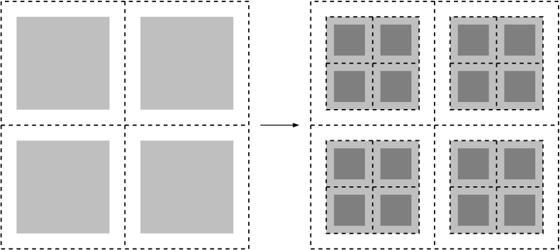
Figure 3. We draw two bisecting steps of the construction of the nested almost coverings of $\Lambda_{N}$, going say from level $j-1$ to $j$ and from level $j$ to $j+1$ in the preliminary version of the construction (that is before inversion: but of course we can view it the other way around ). The dashed lines in the two figures mark a portion of the conditioning grid, but they are also the boundary of boxes: notably on the left the largest cube (square in the figure) delimited by dashed line is one of the $\widetilde{B}$ boxes at level $j-1$, say $\widetilde{B}_{j-1,k_{0}}$. This box contains $2^{d}$ boxes of level $j$: they are denoted by $\widetilde{B}_{j,k}$, $k\in\llbracket 2^{d}k_{0}+1,2^{d}k_{0}+2^{d}\rrbracket$. This operation is then repeated in the drawing in the right and if we choose one of this boxes, say $\widetilde{B}_{j,k_{1}}$, the next level boxes inside $\widetilde{B}_{j,k_{1}}$ are $\widetilde{B}_{j+1,k}$ with $k\in\llbracket 2^{d}k_{1}+1,2^{d}k_{1}+2^{d}\rrbracket$.

Now we introduce for $j=0,1,\ldots,J$ the decreasing sequence of sets (that are all unions of hypercubes) with $\widetilde{D}_{0}:=\Lambda_{N}$ and for $j=1,\ldots,J$

$$\widetilde{D}_{j}\,:=\,\bigcup_{\widetilde{B}\in\widetilde{\mathcal{C}}_{j}}\widetilde{B}\,.$$ (5.6)

Now we reverse the order by introducing for $j=0,\ldots,J$

$$N_{j}\,:=\,\widetilde{N}_{J-j},\ \ \ \ B_{j}\,:=\,\widetilde{B}_{J-j},\ \ \ \ \ D_{j}:=\widetilde{D}_{J-j},\ \ \ \ G_{j}\,:=\,\widetilde{G}_{J-j},\ \ \ \ {\mathbb{G}}_{j}\,:=\,\widetilde{\mathbb{G}}_{J-j}\,.$$ (5.7)

Note that with this order reversing, $N_{j}$ is close to $2^{j}N_{0}$ and $N_{0}$ does not depend much on $N$ (cf. (5.4)), namely $h^{2/d}N_{0}/(\log(1/h))^{2/d}\in[7,15]$. Furthermore, with our construction, the fraction of $\Lambda_{N}$ which is not covered by level zero boxes $B_{0,k}$ is small. The content of this paragraph is made more precise and quantitative by:

Lemma 5.3.

With the notations specified above, for every $\varkappa>0$ there exists $C_{\varkappa}>0$ and $h_{0}>0$ such that for every $j\geq 1$ and every $h\in(0,h_{0}]$ we have

$$2^{j}N_{0}\,\leq\,N_{j}\,\leq\,(1+C_{\varkappa}N^{-\varkappa}_{0})2^{j}N_{0}\,.$$ (5.8)

In particular we have for $C^{\prime}_{\varkappa}=2dC_{\varkappa}$

$$\frac{\left|\bigcup_{k=1}^{2^{dJ}}B_{0,k}\right|}{N^{d}}\geq\left(1-C^{\prime}_{\varkappa}N_{0}^{-\varkappa}\right)\,.$$ (5.9)

Proof.

The lower bound in (5.8) is immediate since (5.2) implies $N_{j}\geq 2N_{j-1}$. As for the upper bound in (5.8), by definition $N_{0}=\widetilde{N}_{J}\geq 7((1/h)\log(1/h))^{2/d}$ (recall (5.4)), (5.2) implies that, if $h$ is sufficiently small, for every $j\geq 1$ we have

$$N_{j}\leq 2N_{j-1}+10(N_{j-1})^{1-\varkappa}\,=\,2N_{j-1}\left(1+5N_{j-1}^{-\varkappa}\right)\,.$$ (5.10)

Hence iterating and using the lower bound we obtain

$$\frac{N_{j}}{N_{0}}\leq 2^{j}\prod_{i=1}^{j}\left(1+5N^{-\varkappa}_{i-1}\right)\leq 2^{j}\prod_{i=0}^{\infty}\left(1+5(2^{i}N_{0})^{-\varkappa}\right)\,\leq\,2^{j}\left(1+C_{\varkappa}N_{0}^{-\varkappa}\right)\,,$$ (5.11)

with $C_{\varkappa}=6/(1-2^{-\varkappa})$. Therefore (5.8) is proven. The inequality (5.9) comes from the fact that from (5.8) we have

$$\frac{\left|\bigcup_{k=1}^{2^{dJ}}B_{0,k}\right|}{N^{d}}=\left(\frac{2^{J}N_{0}}{N_{J}}\right)^{d}\geq(1+C_{\varkappa}N^{-\varkappa}_{0})^{-d}\,,$$ (5.12)

from which the result follows. ∎

Finally, we divide the level-$0$ boxes, whose edge length $N_{0}$ satisfies (because of (5.4))

$$7(\log(1/h)/h)^{2/d}\,\leq\,N_{0}\,\leq\,15(\log(1/h)/h)^{2/d}\,,$$ (5.13)

into $6^{d}$ cubes of edge length $\lfloor N_{0}/6\rfloor$. More precisely $\mkern 1.5mu\overline{\mkern-1.5muB\mkern-1.5mu}\mkern 1.5mu_{6^{d}k+i}$, $i=1,\dots,6^{d}$ are obtained by dividing $B_{0,k}$, see Fig. 4. We set $\mkern 1.5mu\overline{\mkern-1.5muN\mkern-1.5mu}\mkern 1.5mu_{h}=\lfloor N_{0}/6\rfloor$ and set $\mkern 1.5mu\overline{\mkern-1.5mu{\mathcal{C}}\mkern-1.5mu}\mkern 1.5mu_{0}:=\{\mkern 1.5mu\overline{\mkern-1.5muB\mkern-1.5mu}\mkern 1.5mu_{l},l\in\llbracket 1,6^{d}2^{dJ}\rrbracket\}$. Note that (5.9) is also valid for $\bigcup_{l}\mkern 1.5mu\overline{\mkern-1.5muB\mkern-1.5mu}\mkern 1.5mu_{l}$, possibly increasing the value of $C^{\prime}_{\varkappa}$. Moreover $\mkern 1.5mu\overline{\mkern-1.5muN\mkern-1.5mu}\mkern 1.5mu_{h}$ depends on $N$ only mildly: in fact from (5.4) we have

$$(\log(1/h)/h)^{2/d}\,\leq\,\mkern 1.5mu\overline{\mkern-1.5muN\mkern-1.5mu}\mkern 1.5mu_{h}\leq 3(\log(1/h)/h)^{2/d}\,.$$ (5.14)

We refer to $\mkern 1.5mu\overline{\mkern-1.5muB\mkern-1.5mu}\mkern 1.5mu_{l}$ as an elementary box and to $B_{0,k}$ as a level-$0$ box.

We let

$$K\,:=\,2^{dJ}\ \textrm{ and }\mkern 1.5mu\overline{\mkern-1.5muK\mkern-1.5mu}\mkern 1.5mu\,:=\,6^{d}2^{dJ}\,,$$ (5.15)

denote the number of as level-$0$ boxes and elementary boxes respectively.

5.2. Control of the contact density in elementary boxes

For $k\in\llbracket 1,\mkern 1.5mu\overline{\mkern-1.5muK\mkern-1.5mu}\mkern 1.5mu\rrbracket$ let us define $\zeta(k)$ to be the contact fraction inside $\mkern 1.5mu\overline{\mkern-1.5muB\mkern-1.5mu}\mkern 1.5mu_{k}$.

$$\zeta(k):=\frac{1}{\mkern 1.5mu\overline{\mkern-1.5muN\mkern-1.5mu}\mkern 1.5mu_{h}^{d}}\sum_{x\in\mkern 1.5mu\overline{\mkern-1.5muB\mkern-1.5mu}\mkern 1.5mu_{k}}\mathbf{1}_{[-1,1]}(\phi(x))\,,$$ (5.16)

and let ${\mathcal{C}}(N,\delta)$ be the event that most boxes have a contact fraction reasonably close to the optimal value $p_{h}=2\chi(\beta)h$

$${\mathcal{C}}(N,\delta):=\left\{\#\left\{k\in\llbracket 1,\mkern 1.5mu\overline{\mkern-1.5muK\mkern-1.5mu}\mkern 1.5mu\rrbracket\ :\ \frac{\zeta(k)}{\chi(\beta)h}\not\in[1,3]\right\}\,\leq\,\delta\mkern 1.5mu\overline{\mkern-1.5muK\mkern-1.5mu}\mkern 1.5mu\right\}\,.$$ (5.17)

In the end $\delta$ will be chosen proportional to $\varepsilon$. Our first step is to prove that ${\mathcal{C}}(N,\delta)$ has probability close to one.

Lemma 5.4.

Choose an arbitrary value of $\delta>0$. Then there exists $h_{0}>0$ such that for $h\in(0,h_{0}]$ there exists $c=c(h)>0$ and $N_{h}>0$ such that for $h\in(0,h_{0}]$ and $N\geq N_{h}$ we have

$${\mathbb{E}}\left[{\mathbf{P}}_{N,\omega,\beta,h}\left({\mathcal{C}}(N,\delta)^{\complement}\right)\right]\,=e^{-c(h)\delta N^{d}}.$$ (5.18)

Remark 5.5.

The result would be valid also replacing $[1,3]$ by an arbitrarily small interval centered at $2$, but this is useless for the rest of the proof and, with our choice, we avoid introducing one more parameter.

Proof.

We are going to prove an upper bound on $Z_{N,\omega,\beta,h}\left({\mathcal{C}}(N,\delta)^{\complement}\right)$ which shows that it is typically much smaller than $Z_{N,\omega,\beta,h}$. More precisely, by the Markov inequality it is sufficient to show that for every $h>0$ small there exists $\theta\in(0,1)$ such that

$$\limsup_{N\to\infty}\frac{1}{\theta N^{d}}\log{\mathbb{E}}\left[Z_{N,\omega,\beta,h}\left({\mathcal{C}}(N,\delta)^{\complement}\right)^{\theta}\right]<\textsc{f}(\beta,h).$$ (5.19)

We decompose $Z_{N,\omega,\beta,h}\left({\mathcal{C}}(N,\delta)^{\complement}\right)$ according to the position of atypical density blocks. Given $I\subset\llbracket 1,\mkern 1.5mu\overline{\mkern-1.5muK\mkern-1.5mu}\mkern 1.5mu\rrbracket$ we set

$${\mathcal{A}}_{I}\,:=\,\left\{\left\{k\ :\ \left|\zeta(k)-2\chi(\beta)h\right|\,\leq\,{\chi(\beta)}h\right\}=I\right\}\,,$$ (5.20)

so ${\mathcal{C}}(N,\delta)^{\complement}$ coincides with the union of the events ${\mathcal{A}}_{I}$ with $|I|\geq\delta\mkern 1.5mu\overline{\mkern-1.5muK\mkern-1.5mu}\mkern 1.5mu$. We then observe that for $\theta\in(0,1]$

$$Z_{N,\omega,\beta,h}\left({\mathcal{C}}(N,\delta)^{\complement}\right)^{\theta}\leq\sum_{\{I\ :\ |I|\geq\delta\mkern 1.5mu\overline{\mkern-1.5muK\mkern-1.5mu}\mkern 1.5mu\}}Z_{N,\omega,\beta,h}\left({\mathcal{A}}_{I}\right)^{\theta}\,,$$ (5.21)

where we have used the elementary inequality $(\sum_{j}a_{j})^{\theta}\leq\sum_{j}a_{j}^{\theta}$ that holds for $a_{j}>0$. Therefore

$${\mathbb{E}}\left[Z_{N,\omega,\beta,h}\left({\mathcal{C}}(N,\delta)^{\complement}\right)^{\theta}\right]\leq 2^{\mkern 1.5mu\overline{\mkern-1.5muK\mkern-1.5mu}\mkern 1.5mu}\max_{|I|\geq\delta\mkern 1.5mu\overline{\mkern-1.5muK\mkern-1.5mu}\mkern 1.5mu}{\mathbb{E}}\left[Z_{N,\omega,\beta,h}\left({\mathcal{A}}_{I}\right)^{\theta}\right].$$ (5.22)

Now we can use the fact that $\mkern 1.5mu\overline{\mkern-1.5muK\mkern-1.5mu}\mkern 1.5mu\leq(N/\mkern 1.5mu\overline{\mkern-1.5muN\mkern-1.5mu}\mkern 1.5mu_{h})^{d}$ (simply because the boxes are disjoint), and we obtain that

$$\frac{1}{\theta N^{d}}\log{\mathbb{E}}\left[Z_{N,\omega,\beta,h}\left({\mathcal{C}}(N,\delta)^{\complement}\right)^{\theta}\right]\leq\frac{\log 2}{\theta\mkern 1.5mu\overline{\mkern-1.5muN\mkern-1.5mu}\mkern 1.5mu^{d}_{h}}+\frac{1}{\theta N^{d}}\max_{|I|\geq\delta\mkern 1.5mu\overline{\mkern-1.5muK\mkern-1.5mu}\mkern 1.5mu}\log{\mathbb{E}}\left[Z_{N,\omega,\beta,h}\left({\mathcal{A}}_{I}\right)^{\theta}\right].$$ (5.23)

If one sets $\theta=\theta_{h}:=(\log 1/h)^{-1}$, the first term on the right-hand side  is $O(h^{2}(\log 1/h)^{-1})$. Hence we can conclude if we show that there exists $c>0$ such that for $h$ sufficiently small

$$\frac{1}{\theta_{h}N^{d}}\max_{|I|\geq\delta\mkern 1.5mu\overline{\mkern-1.5muK\mkern-1.5mu}\mkern 1.5mu}\log{\mathbb{E}}\left[Z_{N,\omega,\beta,h}\left({\mathcal{A}}_{I}\right)^{\theta_{h}}\right]\leq\chi(\beta)(1-c\delta)h^{2}\,.$$ (5.24)

For this we use the following technical lemma, whose proof is postponed till the end of the proof we are developing.

Lemma 5.6.

Recall that $\xi_{x}=e^{h+\beta\omega_{x}-\lambda(\beta)}-1$. For any measure on ${\mathbf{P}}_{\Lambda}$ on $\{0,1\}^{\Lambda}$ and every $\theta\in(0,1)$ we have for every $h\geq 0$ that

$${\mathbb{E}}\left[{\mathbf{E}}_{\Lambda}\left[\prod_{\{x\ :\ \delta_{x}=1\}}(1+\xi_{x})\right]^{\theta}\right]\leq\left(\max_{p\in(0,1]}{\mathbb{E}}\left[(1+p\xi)^{\theta}\right]\right)^{|\Lambda|}.$$ (5.25)

In the limit where $\theta$ and $h$ tend to zero we have

$$\frac{1}{\theta}\max_{p\in(0,1)}\log{\mathbb{E}}\left[(1+p\xi)^{\theta}\right]=\chi(\beta)h^{2}+O(h^{2}\theta)+O(h^{3}).$$ (5.26)

If furthermore ${\mathbf{P}}_{\Lambda}$ is such that for $\eta>0$ and $h>0$

$${\mathbf{P}}_{\Lambda}\left(\left|\frac{1}{|\Lambda|}\sum_{x\in\Lambda}\delta_{x}-2\chi(\beta)h\right|\geq\eta h\right)\,=\,1\,,$$ (5.27)

then there exist $C=C_{\beta}>0$, $h_{0}=h_{0,\beta,\eta}$ and $\theta_{0}=\theta_{0,\beta}$ such that for all $h\in(0,h_{0}]$ and $\theta\in(0,\theta_{0}]$ and for all $\Lambda$

$$\frac{1}{\theta|\Lambda|}\log{\mathbb{E}}\left[{\mathbf{E}}_{\Lambda}\left[\prod_{\{x\ :\ \delta_{x}=1\}}(1+\xi_{x})\right]^{\theta}\right]\,\leq\,\chi(\beta)\left(1-\frac{\eta^{2}}{4\chi(\beta)^{2}}\right)h^{2}+\frac{\log 2}{\theta|\Lambda|}+C(h^{2}\theta+h^{3})\,.$$ (5.28)

Remark 5.7.

The inequality (5.28) is valid for all size of boxes. However it provides a better bound than (5.26) only if $\theta|\Lambda|$ is much larger than $h^{-2}$.

Consider $I\subset\llbracket 1,\mkern 1.5mu\overline{\mkern-1.5muK\mkern-1.5mu}\mkern 1.5mu\rrbracket$ with $|I|\geq\delta\mkern 1.5mu\overline{\mkern-1.5muK\mkern-1.5mu}\mkern 1.5mu$. Let $k_{1}\leq\dots\leq k_{|I|}$ denote the elements of $I$. We can prove by induction that for every $j\leq|I|$

$$T_{1}(I,j)\,:=\,\frac{1}{\theta_{h}}\log{\mathbb{E}}\left[\left({\mathbf{E}}_{N}\left[e^{\sum_{x\in\bigcup_{1\leq i\leq j}\mkern 1.5mu\overline{\mkern-1.5muB\mkern-1.5mu}\mkern 1.5mu_{k_{i}}}(\beta\omega_{x}-\lambda(\beta)+h)\delta_{x}}\ \bigg{|}\ {\mathcal{A}}_{I}\right]\right)^{\theta_{h}}\right]\,\leq\,\frac{j}{2}\chi(\beta)h^{2}\mkern 1.5mu\overline{\mkern-1.5muN\mkern-1.5mu}\mkern 1.5mu_{h}^{d}.$$ (5.29)

The result for $j=1$ is a direct consequence of (5.28): we work with $\eta=\chi(\beta)$ and then we use that $1/(\mkern 1.5mu\overline{\mkern-1.5muN\mkern-1.5mu}\mkern 1.5mu_{h}^{d}\theta_{h})=O(h^{2}/\log(1/h))\ll h^{2}$, so that the term $(\log 2)/(\theta_{h}|\Lambda|)$, as well as the term $C(h^{2}\theta_{h}+h^{3})$, can be absorbed into the leading order, for $h$ sufficiently small. Now for $j>1$, we just need to apply (5.28) to the measure $\mu$ defined by

$$\mu(A):=\frac{{\mathbf{E}}_{N}\left[e^{\sum\limits_{x\in\left(\cup_{1\leq i\leq j-1}\mkern 1.5mu\overline{\mkern-1.5muB\mkern-1.5mu}\mkern 1.5mu_{k_{i}}\right)}(\beta\omega_{x}-\lambda(\beta)+h)\delta_{x}}\mathbf{1}_{A}\ \bigg{|}\ {\mathcal{A}}_{I}\right]}{{\mathbf{E}}_{N}\left[e^{\sum\limits_{x\in\left(\cup_{1\leq i\leq j-1}\mkern 1.5mu\overline{\mkern-1.5muB\mkern-1.5mu}\mkern 1.5mu_{k_{i}}\right)}(\beta\omega_{x}-\lambda(\beta)+h)\delta_{x}}\ \bigg{|}\ {\mathcal{A}}_{I}\right]}\,.$$ (5.30)

We obtain that

$$\log{\mathbb{E}}\left[\left(\frac{{\mathbf{E}}_{N}\left[e^{\sum\limits_{x\in\left(\cup_{1\leq i\leq j}\mkern 1.5mu\overline{\mkern-1.5muB\mkern-1.5mu}\mkern 1.5mu_{k_{i}}\right)}(\beta\omega_{x}-\lambda(\beta)+h)\delta_{x}}\ \ \bigg{|}\ {\mathcal{A}}_{I}\right]}{{\mathbf{E}}_{N}\left[e^{\sum\limits_{x\in\left(\cup_{1\leq i\leq j-1}\mkern 1.5mu\overline{\mkern-1.5muB\mkern-1.5mu}\mkern 1.5mu_{0,k_{i}}\right)}(\beta\omega_{x}-\lambda(\beta)+h)\delta_{x}}\ \ \bigg{|}\ {\mathcal{A}}_{I}\right]}\right)^{\theta_{h}}\right]\\ \\ =\log{\mathbb{E}}\left[\mu\left(e^{\sum_{x\in\mkern 1.5mu\overline{\mkern-1.5muB\mkern-1.5mu}\mkern 1.5mu_{k_{j}}}(\beta\omega_{x}-\lambda(\beta)+h)\delta_{x}}\right)^{\theta_{h}}\right]\,\leq\,\frac{1}{2}\theta_{h}\mkern 1.5mu\overline{\mkern-1.5muN\mkern-1.5mu}\mkern 1.5mu^{d}_{h}\chi(\beta)h^{2}$$ (5.31)

where the inequality is obtained by applying (5.28), in the same way as for the case $j=1$, when averaging with respect to $(\omega_{x})_{x\in\mkern 1.5mu\overline{\mkern-1.5muB\mkern-1.5mu}\mkern 1.5mu_{k_{j}}}$. This completes the induction argument and (5.29) is proven.

Using the same trick and (5.25)-(5.26) we obtain that

$$T_{2}(I)\,:=\,\frac{1}{\theta_{h}}\log{\mathbb{E}}\left[\left(\frac{{\mathbf{E}}_{N}\left[e^{\sum_{x\in\mathring{\Lambda}_{N}}(\beta\omega_{x}-\lambda(\beta)+h)\delta_{x}}\ \ \Big{|}\ {\mathcal{A}}_{I}\right]}{{\mathbf{E}}_{N}\left[e^{\sum_{x\in\bigcup_{i\in I}\mkern 1.5mu\overline{\mkern-1.5muB\mkern-1.5mu}\mkern 1.5mu_{k_{i}}}(\beta\omega_{x}-\lambda(\beta)+h)\delta_{x}}\ \ \Big{|}\ {\mathcal{A}}_{I}\right]}\right)^{\theta_{h}}\right]\\ \leq\,\left[(N-1)^{d}-|I|\mkern 1.5mu\overline{\mkern-1.5muN\mkern-1.5mu}\mkern 1.5mu^{d}_{h}\right](\chi(\beta)h^{2}+C\theta_{h}h^{2})\,.$$ (5.32)

Finally, combining (5.29) and (5.32), by apply the Cauchy-Schwarz inequality we obtain

$$\begin{split}\frac{2}{\theta_{h}}\log{\mathbb{E}}\left[Z_{N,\omega,\beta,h}\left({\mathcal{A}}_{I}\right)^{(\theta_{h}/2)}\right]&\leq\,\frac{2}{\theta_{h}}\log{\mathbb{E}}\left[\left({{\mathbf{E}}_{N}\left[e^{\sum_{x\in\mathring{\Lambda}_{N}}(\beta\omega_{x}-\lambda(\beta)+h)\delta_{x}}\ \ \Big{|}\ {\mathcal{A}}_{I}\right]}\right)^{\theta_{h}/2}\right]\\ &\leq\,T_{1}(I,|I|)+T_{2}(I)\,\leq\,\chi(\beta)h^{2}\left(N^{d}-\frac{1}{2}|I|\mkern 1.5mu\overline{\mkern-1.5muN\mkern-1.5mu}\mkern 1.5mu^{d}_{h}\right)+C\theta_{h}h^{2}N^{d}\\ &\leq\,\left(1-\frac{\delta}{3}\right)\chi(\beta)h^{2}N^{d}\,,\end{split}$$ (5.33)

which is (5.24) with $c=1/3$, except for the (clearly irrelevant) fact that $\theta_{h}$ is replaced by $\theta_{h}/2$. ∎

Proof of Lemma 5.6.

The inequality (5.25) can be proven using the approach that lead to (2.2), but we give here a different proof. We proceed by induction on $N=|\Lambda|$. Note that we can assume without loss of generality that $\Lambda:=\llbracket 0,N\rrbracket$ and write ${\mathbf{E}}_{N}$ for ${\mathbf{E}}_{\Lambda}$. The result is obvious for $N=0$. Now given $N\geq 1$ set

$$p_{N}(\xi_{1},\dots,\xi_{N-1}):=\frac{{\mathbf{E}}_{N}\left[\prod_{\{x\in\llbracket 1,N-1\rrbracket\ :\ \delta_{x}=1\}}\left(1+\xi_{x}\right)\delta_{N}\right]}{{\mathbf{E}}_{N}\left[\prod_{\{x\in\llbracket 1,N-1\rrbracket\ :\ \delta_{x}=1\}}\left(1+\xi_{x}\right)\right]}\ ,$$ (5.34)

together with

$$Z_{N}(\xi):={\mathbf{E}}_{N}\left[\prod_{\{x\in\llbracket 1,N\rrbracket\ :\ \delta_{x}=1\}}(1+\xi_{x})\right]\ \ \ \text{ and }\ \ \ \widetilde{Z}_{N}(\xi):={\mathbf{E}}_{N}\left[\prod_{\{x\in\llbracket 1,N-1\rrbracket\ :\ \delta_{x}=1\}}(1+\xi_{x})\right].$$ (5.35)

Note that

$$Z_{N}(\xi)\,=\,\widetilde{Z}_{N}(\xi)(1+p_{N}\xi_{N})\,,$$ (5.36)

and by raising both sides to the power $\theta$ and taking the average with respect to $\xi_{N}$ we obtain

$${\mathbb{E}}\left[Z^{\theta}_{N}(\xi)\ \big{|}\ (\xi_{x})_{1\leq x\leq N-1}\right]=\widetilde{Z}_{N}^{\theta}(\xi){\mathbb{E}}\left[(1+p_{N}\xi_{N})^{\theta}\right]\leq\widetilde{Z}_{N}^{\theta}(\xi)\max_{p\in(0,1]}{\mathbb{E}}\left[(1+p\xi)^{\theta}\right]\,,$$ (5.37)

and by taking the average with respect to all other variables on both sides we obtain that

$${\mathbb{E}}\left[Z^{\theta}_{N}(\xi)\right]\,\leq\,{\mathbb{E}}\left[\widetilde{Z}^{\theta}_{N}(\xi)\right]\max_{p\in(0,1]}{\mathbb{E}}\left[(1+p\xi)^{\theta}\right]\,.$$ (5.38)

We can now take the supremum over ${\mathbf{P}}_{N}$ and we can conclude the induction step because

$$\sup_{{\mathbf{P}}_{N}}{\mathbb{E}}\left[\widetilde{Z}^{\theta}_{N}(\xi)\right]\,=\,\sup_{{\mathbf{P}}_{N-1}}{\mathbb{E}}\left[Z^{\theta}_{N-1}(\xi)\right]\,.$$ (5.39)

The bound (5.25) is therefore established.

As for the optimizing problem (5.26) we can proceed as for Proposition 2.2 using Taylor expansion and showing first that $p_{h,\theta}$ tends to $0$, then that $p_{h,\theta}\sim 2\chi(\beta)h$, then $p_{h,\theta}=2\chi(\beta)h+O(\theta h)+O(h^{2})$ and then the final claim. We do not detail these steps.

For what concerns (5.28) (recall that we are therefore assuming (5.27)), at the cost of loosing a factor two in the estimate on ${\mathbb{E}}[Z^{\theta}_{N}]$ we can assume that one of the following holds

$${\mathbf{P}}_{N}\left(\sum_{x=1}^{N}\delta_{x}\geq(2\chi(\beta)+\eta)hN\right)\,=\,1\,\text{ or }{\mathbf{P}}_{N}\left(\sum_{x=1}^{N}\delta_{x}\leq(2\chi(\beta)-\eta)hN\right)\,=\,1\,.$$ (5.40)

Using Hölder inequality we have that for every positive random variable $g$

$${\mathbb{E}}\left[Z_{N}^{\theta}\right]\,\leq\,{\mathbb{E}}[Z_{N}g^{\theta-1}]^{\theta}{\mathbb{E}}[g^{\theta}]^{1-\theta}\,.$$ (5.41)

Now we set $g=\prod_{x\in\llbracket 1,N\rrbracket}(1+q\xi^{\prime})^{\frac{1}{1-\theta}}$ with $\xi^{\prime}=e^{\beta\omega-\lambda(\beta)}-1$ (using $\xi$ instead of $\xi^{\prime}$ would give an analogous result but computations are easier with $\xi^{\prime}$). We are going to set $q=q_{\pm}:=(2\chi(\beta)\pm\eta)h$ depending on which assumption we have on the contact fraction.

The following asymptotic statements hold in the limit where both $q$ and $\theta$ go to zero

$$\begin{split}{\mathbb{E}}\left[(1+q\xi^{\prime})^{-1}\right]&=1+q^{2}\mathrm{Var}(\xi^{\prime})+O(q^{3}),\\ {\mathbb{E}}\left[(1+\xi^{\prime})(1+q\xi)^{-1}\right]&=1-q\mathrm{Var}(\xi^{\prime})+O(q^{2}),\\ {\mathbb{E}}\left[(1+q\xi^{\prime})^{\frac{\theta}{1-\theta}}\right]&=1-\frac{\theta(1-2\theta)}{2(1-\theta)^{2}}\mathrm{Var}(\xi^{\prime})q^{2}+O(\theta q^{3}).\end{split}$$ (5.42)

Note in particular performing a second order expansion in $h$ that for fixed $\eta$ with our choice of $q$ we have for $h$ sufficiently small (depending on $\eta$ and on $\beta$)

$$\begin{split}e^{h}{\mathbb{E}}\left[(1+\xi^{\prime})(1+q_{-}\xi^{\prime})^{-1}\right]\,&\geq\,{\mathbb{E}}\left[(1+q_{-}\xi^{\prime})^{-1}\right],\\ e^{h}{\mathbb{E}}\left[(1+\xi^{\prime})(1+q_{+}\xi^{\prime})^{-1}\right]\,&\leq\,{\mathbb{E}}\left[(1+q_{+}\xi^{\prime})^{-1}\right].\end{split}$$ (5.43)

If $\sum_{x\in\llbracket 0,N\rrbracket}\delta_{x}\leq Nq_{-}$, ${\mathbf{P}}_{N}$-a.s. we can replace $\sum\delta_{x}$ by its upper bound $q_{-}|\Lambda|$ and altogether we obtain

$${\mathbb{E}}\left[Z_{N}^{\theta}\right]\leq\left(e^{h}{\mathbb{E}}\left[(1+\xi^{\prime})(1+q_{-}\xi)^{-1}\right]\right)^{q_{-}N\theta}\\ \times\left({\mathbb{E}}\left[(1+q_{-}\xi)^{-1}\right]\right)^{(1-q_{-})N\theta}\left({\mathbb{E}}\left[(1+q_{-}\xi^{\prime})^{\frac{\theta}{1-\theta}}\right]\right)^{N(1-\theta)}.$$ (5.44)

Hence applying (5.43) we obtain

$$\frac{1}{N\theta}\log{\mathbb{E}}\left[Z_{N}^{\theta}\right]\leq q_{-}h-\frac{q^{2}_{-}}{2}\mathrm{Var}(\xi^{\prime})+O(\theta q^{2})+O(q^{3})\\ =\,\left(\chi(\beta)-\frac{\eta^{2}}{4\chi(\beta)}\right)h^{2}+O(h^{2}\theta)+O(h^{3}).$$ (5.45)

In the same manner when $\sum_{x\in\llbracket 0,N\rrbracket}\delta_{x}\geq Nq_{+}$, ${\mathbf{P}}_{N}$-a.s. we have

$${\mathbb{E}}\left[Z_{N}^{\theta}\right]\leq\left(e^{h}{\mathbb{E}}\left[(1+\xi^{\prime})(1+q_{+}\xi)^{-1}\right]\right)^{q_{+}N\theta}\\ \times\left({\mathbb{E}}\left[(1+q_{+}\xi)^{-1}\right]\right)^{(1-q_{+})N\theta}\left({\mathbb{E}}\left[(1+q_{+}\xi^{\prime})^{\frac{\theta}{1-\theta}}\right]\right)^{N(1-\theta)}.$$ (5.46)

and we obtain

$$\frac{1}{N\theta}\log{\mathbb{E}}\left[Z_{N}^{\theta}\right]\leq q_{+}h-\frac{q^{2}_{+}}{2}\mathrm{Var}(\xi^{\prime})+O(\theta q^{2})+O(q^{3})\\ =\,\left(\chi(\beta)-\frac{\eta^{2}}{4\chi(\beta)}\right)h^{2}+O(h^{2}\theta)+O(h^{3}).$$ (5.47)

This completes the proof of Lemma 5.6. ∎

5.3. The main body of the argument (Proof of Proposition 5.1)

We start by an important preliminary result. By using the control we have on the local contact density and on the free energy, we are going to show that if the probability of a sequence of events decays exponentially in the volume size under ${\mathbf{P}}_{N}$ with a rate suitably controlled from below, then it also decays exponentially under ${\mathbf{P}}_{N,\omega,\beta,h}$. Said differently, the result we are going to state allows to neglect the environment and to reduce the estimates to Gaussian field estimates.

Lemma 5.8.

Recall $\varepsilon_{d}>0$ from Propositon 3.1. Consider for $h\leq h_{0}$, $N$ larger than a suitable $N_{0}(h)$ and a sequence of events $A_{N}$ such that ${\mathbf{P}}_{N}(A_{N})\leq\exp(-h^{2+\eta}N^{d})$, with $\eta\in(0,\varepsilon_{d})$. Then there exists $h^{\prime}_{0}>0$ and $N^{\prime}_{0}(h,\omega)$ such that for every $h\leq h^{\prime}_{0}$ and $N\geq N^{\prime}_{0}(h)$

$${\mathbf{P}}_{N,\omega,\beta,h}\left(A_{N}\right)\,\leq\,\exp(-N^{d}h^{2+\eta}/4)\,.$$ (5.48)

Proof.

Because $N^{-d}\log Z_{N,\omega,\beta,h}$ converges, it is sufficient to show that (recall (4.5))

$$\frac{1}{N^{d}}\log Z_{N,\omega,\beta,h}\left(A_{N}\right)\,\leq\,\textsc{f}(\beta,h)-h^{2+\eta}/3\,.$$ (5.49)

We are going to show first that

$$\frac{1}{N^{d}}{\mathbb{E}}\left[\log Z_{N,\omega,\beta,h}\left(A_{N}\right)\right]\leq\textsc{f}(\beta,h)-h^{2+\eta}/2.$$ (5.50)

To see this, we note that we have (using Proposition 2.3 for ${\mathbf{P}}_{N}(\ \cdot\ |\ A_{N})$ and keeping into account Remark 2.4)

$${\mathbb{E}}\left[\log Z_{N,\omega}\left(A_{N}\right)\right]=\log{\mathbf{P}}_{N}(A_{N})+{\mathbb{E}}\log{\mathbf{E}}_{N}\left[e^{\sum_{x\in\mathring{\Lambda}_{N}}(\beta\omega_{x}-\lambda(\beta)+h)\delta_{x}}\ \big{|}\ A_{N}\right]\\ \leq\,-N^{d}h^{2+\eta}+|\mathring{\Lambda}_{N}|(h^{2}\chi(\beta)+C_{\beta}h^{3})\,.$$ (5.51)

We have used $Z_{N}$ as a shortcut for $Z_{N,\omega,\beta,h}$ and we recall that $\mathring{\Lambda}_{N}=\llbracket 1,N-1\rrbracket^{d}$, hence $|\mathring{\Lambda}_{N}|\leq N^{d}$. Now in view of Proposition 3.1, (5.51) implies that (5.50) holds for $h$ sufficiently small.

Now to conclude we only need to show that $\log Z_{N,\omega}(A_{N})$ is concentrated around its mean. This follows from a standard concentration argument, for which we introduce a cut-off $M_{N}:=N^{d/6}$ on the disorder variables $\mkern 1.5mu\overline{\mkern-1.5mu\omega\mkern-1.5mu}\mkern 1.5mu_{x}:=\omega_{x}\mathbf{1}_{\{|\omega_{x}|\leq M_{N}\}}$. A union bound and the finiteness of the exponential moment of all orders for $\omega$ implies that for $N$ sufficiently large we have

$${\mathbb{P}}\left(\exists x\in\Lambda_{N},\ |\omega_{x}|\geq M_{N}\right)\,\leq\,e^{-N^{d/6}}\,.$$ (5.52)

Therefore, by Azuma’s inequality applied to the martingale $({\mathbb{E}}[\log\mkern 1.5mu\overline{\mkern-1.5muZ\mkern-1.5mu}\mkern 1.5mu_{N,\mkern 1.5mu\overline{\mkern-1.5mu\omega\mkern-1.5mu}\mkern 1.5mu}(A_{N})\ |\ {\mathcal{G}}_{n}])^{|\mathring{\Lambda}_{N}|}_{n=0}$, where ${\mathcal{G}}_{n}:=\sigma(\omega_{x_{i}},i\leq n)$ and $x_{1},\dots,x_{|\mathring{\Lambda}_{N}|}$ is an arbitrary enumeration of $\mathring{\Lambda}_{N}$, we obtain that there

$${\mathbb{P}}\left(|\log Z_{N,\mkern 1.5mu\overline{\mkern-1.5mu\omega\mkern-1.5mu}\mkern 1.5mu}(A_{N})-{\mathbb{E}}[\log Z_{N,\mkern 1.5mu\overline{\mkern-1.5mu\omega\mkern-1.5mu}\mkern 1.5mu}(A_{N})]|\geq u\right)\,\leq\,e^{-\frac{cu^{2}}{N^{d}M^{2}_{N}}}\,,$$ (5.53)

with $c=1/(\beta+\lambda(\beta)+h)^{2}$. Applying this for $u=N^{3d/4}$ and using (5.52) to bound the probability of $\{Z_{N,\omega}(A_{N})\neq\{Z_{N,\mkern 1.5mu\overline{\mkern-1.5mu\omega\mkern-1.5mu}\mkern 1.5mu}(A_{N})|\}$ we obtain (for $c^{\prime}=c\wedge 1$)

$${\mathbb{P}}\left(\left|\log Z_{N,\omega}(A_{N})-{\mathbb{E}}[\log Z_{N,\mkern 1.5mu\overline{\mkern-1.5mu\omega\mkern-1.5mu}\mkern 1.5mu}(A_{N})\right|>N^{3d/4}\right)\leq 2e^{-c^{\prime}N^{d/6}}$$ (5.54)

At this point wee can conclude by observing that the difference between ${\mathbb{E}}[\log Z_{N,\mkern 1.5mu\overline{\mkern-1.5mu\omega\mkern-1.5mu}\mkern 1.5mu}(A_{N})]$ and ${\mathbb{E}}[\log Z_{N,\omega}(A_{N})]$ is small: this follows by applying Lemma A.3 with $K=M_{N}$ that yields

$${\mathbb{E}}\left[\left|\log Z_{N,\omega}(A_{N})-\log Z_{N,\mkern 1.5mu\overline{\mkern-1.5mu\omega\mkern-1.5mu}\mkern 1.5mu}(A_{N})\right|\right]\,\leq\,\beta N^{d}{\mathbb{E}}\left[|\omega_{x}|;\,|\omega_{x}|>M_{N}\right]\,\leq\,\exp\left(-N^{d/6}\right)\,,$$ (5.55)

for $N$ sufficiently large, again because all exponential moments of $\omega$ are finite. This completes the proof of Lemma 5.8. ∎

Proof of Proposition 5.1. We aim at applying Lemma 5.8 so to reduce the proof of Proposition 5.1 to proving a statement about ${\mathbf{P}}_{N}$. However this fails if applied directly to ${\mathcal{D}}(N,\varepsilon)$ because ${\mathbf{P}}_{N}({\mathcal{D}}(N,\varepsilon))$ does not decrease exponentially in the volume (due to the massless character of the LFF, see e.g. [5]). However, we will show that the event ${\mathcal{C}}(N,\delta)\cap{\mathcal{D}}(N,\varepsilon)$ does not have this drawback and Lemma 5.4 assures that we can limit ourselves to studying this event. More formally, thanks to Lemma 5.4 and Lemma 5.8 it suffices to show that given $\varepsilon>0$ there exist $\delta>0$ and $\eta<\varepsilon_{d}$ such that for $h$ sufficiently small for all $N$ sufficiently large, we have

$$\frac{1}{N^{d}}\log{\mathbf{P}}_{N}\left({\mathcal{C}}(N,\delta)\cap{\mathcal{D}}(N,\varepsilon)\right)\,\leq\,-h^{2+\eta}.$$ (5.56)

To prove (5.56) we are going to use a decomposition of $\phi$ into a field $\psi$ which is independent in each level-$0$ boxes, and a field $\mkern 1.5mu\overline{\mkern-1.5mu\psi\mkern-1.5mu}\mkern 1.5mu$ which displays long range correlation but has a small amplitude.

Recall that ${\mathbb{G}}_{0}$ denotes a grid which isolates each of the boxes at level zero of the hierarchy. By the Markov property of the LFF, we can write

$$\phi=\phi_{\Lambda_{N}}\stackrel{{\scriptstyle\text{(law)}}}{{=}}\psi+\mkern 1.5mu\overline{\mkern-1.5mu\psi\mkern-1.5mu}\mkern 1.5mu\,,$$ (5.57)

where $\mkern 1.5mu\overline{\mkern-1.5mu\psi\mkern-1.5mu}\mkern 1.5mu$ is the harmonic continuation of the restriction of $\phi$ to ${\mathbb{G}}_{0}$, that is the solution of

$$\begin{cases}\Delta\mkern 1.5mu\overline{\mkern-1.5mu\psi\mkern-1.5mu}\mkern 1.5mu(x)=0,\text{ for all }x\in\mathring{\Lambda}_{N}\setminus{\mathbb{G}}_{0},\\ \mkern 1.5mu\overline{\mkern-1.5mu\psi\mkern-1.5mu}\mkern 1.5mu(x)=\phi,\text{ for }x\in{\mathbb{G}}_{0}\,,\end{cases}$$ (5.58)

and $\psi$ a free field on $\mathring{\Lambda}_{N}\setminus{\mathbb{G}}_{0}$ with $0$ boundary condition: therefore $\psi$ is a collection of independent free fields on each of the level-$0$ boxes, and $\mkern 1.5mu\overline{\mkern-1.5mu\psi\mkern-1.5mu}\mkern 1.5mu$ carries all the long range correlations of $\phi$. We are going to reduce the proof of (5.56) to that of the two following facts about $\psi$ and $\mkern 1.5mu\overline{\mkern-1.5mu\psi\mkern-1.5mu}\mkern 1.5mu$ (rigorously stated as Proposition 5.10 and Proposition 5.12 below):

• With very large probability on most level-$0$ boxes $B_{0,k}$, the field $\mkern 1.5mu\overline{\mkern-1.5mu\psi\mkern-1.5mu}\mkern 1.5mu$ is almost flat (in the sense that it is very close to an affine function). We mean by this that the probability of the complement is smaller than $e^{-N^{d}h^{b}}$ for a value of $b<2$: this is largely sufficient because also a value of $b$ slight larger than $2$ would have been sufficient (see Lemma 5.8).

• When $\mkern 1.5mu\overline{\mkern-1.5mu\psi\mkern-1.5mu}\mkern 1.5mu$ is flat on the box $B_{0,k}$, the probability of having both the right number of contact (that is, about $2\mkern 1.5mu\overline{\mkern-1.5muN\mkern-1.5mu}\mkern 1.5mu^{d}_{0}\chi(\beta)h$) in each of the $6^{d}$ elementary boxes inside $B_{0,k}$, and a density of high points is small.

To conclude from these two statements, we only need to use the fact that conditioned to $\mkern 1.5mu\overline{\mkern-1.5mu\psi\mkern-1.5mu}\mkern 1.5mu$, the various level $0$ boxes are independent.

Remark 5.9.

The fact that the $0$ level boxes are separated from the grid of a distance equal (up to integer rounding) to $N_{0}^{1-\varkappa}$ and recalling that $N_{0}\approx(\log(1/h)/h)^{2/d}$, more precisely (5.13), readily yields (use (1.3)) that the variance of $\psi_{x}$ can differ from $\sigma_{d}^{2}$ at most of a term $O(1/N_{0}^{(d-2)(1-\varkappa)})$, that is by $O(h^{c})$ with $c$ a positive constant. In view of the estimates we aim at, these variations of the variance turn out to be irrelevant: details will be given in due times but the reason is simply that for every $b>0$

$$\frac{P\left((1+\epsilon(h)){\mathcal{N}}\geq b\log(1/h)\right)}{P\left({\mathcal{N}}\geq b\log(1/h)\right)}-1\,=\,O\left(h^{c^{\prime}}\right)\,,$$ (5.59)

if $\epsilon(h)=O(h^{c})$. Moreover the distance from the conditioning grid is not only used at level-$0$, but at all levels. However for the higher levels it is used to assure that harmonic extension has a small variance uniformly in the box: the tool we use in that case is Lemma A.4.

Let us give a more quantitative version of $(A)$ and $(B)$. First let us define for $e$ and $g$ two unit vectors (not necessarily distinct) of the canonical base of ${\mathbb{R}}^{d}$ $\nabla_{eg}\mkern 1.5mu\overline{\mkern-1.5mu\psi\mkern-1.5mu}\mkern 1.5mu$ to be the bi-gradient of $\mkern 1.5mu\overline{\mkern-1.5mu\psi\mkern-1.5mu}\mkern 1.5mu$ in directions $e$ and $g$

$$\nabla_{eg}\mkern 1.5mu\overline{\mkern-1.5mu\psi\mkern-1.5mu}\mkern 1.5mu(x)\,:=\,\mkern 1.5mu\overline{\mkern-1.5mu\psi\mkern-1.5mu}\mkern 1.5mu(x+e+g)-\mkern 1.5mu\overline{\mkern-1.5mu\psi\mkern-1.5mu}\mkern 1.5mu(x+e)-\mkern 1.5mu\overline{\mkern-1.5mu\psi\mkern-1.5mu}\mkern 1.5mu(x+g)+\mkern 1.5mu\overline{\mkern-1.5mu\psi\mkern-1.5mu}\mkern 1.5mu(x)\,.$$ (5.60)

Now for $k\in\llbracket 1,K\rrbracket$ (recall $K=2^{dJ}$ is the number of level-$0$ boxes) we set

$$\|\nabla_{eg}\mkern 1.5mu\overline{\mkern-1.5mu\psi\mkern-1.5mu}\mkern 1.5mu\|_{\infty,k}\,:=\,\max_{x\in B_{0,k}}|\nabla_{eg}\mkern 1.5mu\overline{\mkern-1.5mu\psi\mkern-1.5mu}\mkern 1.5mu(x)|\,.$$ (5.61)

Finally we let ${\mathcal{B}}(N,\delta)$ the event that all bi-gradients are small on most boxes, that is

$${\mathcal{B}}(N,\delta)\,:=\,\left\{\left|\{k\in\llbracket 1,K\rrbracket\ :\ \|\nabla_{eg}\mkern 1.5mu\overline{\mkern-1.5mu\psi\mkern-1.5mu}\mkern 1.5mu\|_{\infty,k}\geq N^{-2}_{0}\}\right|\leq\delta K\right\}\,.$$ (5.62)

Here is the result we need on the even ${\mathcal{B}}(N,\delta)$: it is proven in Section 5.5.

Proposition 5.10.

For any $\delta>0$ and for $h$ sufficiently small

$${\mathbf{P}}_{N}\left({\mathcal{B}}(N,\delta)^{\complement}\right)\,\leq\,e^{-N^{d}h^{11/6}}\,.$$ (5.63)

By putting together Lemma 5.8 and Lemma 5.10 we have that for every $\eta>0$, $h$ sufficiently small and $N\geq N_{0}(\omega,\delta,\eta,h)$

$${\mathbf{P}}_{N,\omega,\beta,h}\left({\mathcal{B}}(N,\delta)^{\complement}\right)\,\leq\,e^{-h^{2+\eta}N^{d}}\,.$$ (5.64)

But since $11/6<2$ we can avoid Lemma 5.8 and obtain in a more direct way from Lemma 5.10 that the right-hand side in (5.64) can be improved to $e^{-h^{2-\eta}N^{d}}$, any $\eta<1/6$, but this is irrelevant for what follows.

Remark 5.11.

The reason for us to consider bi-gradient of of $\mkern 1.5mu\overline{\mkern-1.5mu\psi\mkern-1.5mu}\mkern 1.5mu$ instead of $\mkern 1.5mu\overline{\mkern-1.5mu\psi\mkern-1.5mu}\mkern 1.5mu$ or its gradient is that the spatial correlations of the bi-gradient are summable (which is not the case for neither $\mkern 1.5mu\overline{\mkern-1.5mu\psi\mkern-1.5mu}\mkern 1.5mu$ nor for its gradient). The corresponding statement for $\psi$ or for the gradient of $\psi$ would not hold for this reason.

Given $k\in\llbracket 1,K\rrbracket$, and recalling that $\mkern 1.5mu\overline{\mkern-1.5muB\mkern-1.5mu}\mkern 1.5mu_{6^{d}k+i}$, $i=1,\dots,6^{d}$ are disjoint boxes of edge length $\mkern 1.5mu\overline{\mkern-1.5muN\mkern-1.5mu}\mkern 1.5mu_{h}$ located in $B_{0,k}$ we define ${\mathcal{E}}^{(1)}(k)$ to be the event that all elementary boxes in $B_{0,k}$ have a typical contact density. Recalling (5.16) we set

$${\mathcal{E}}^{(1)}(k):=\bigcap_{i=1}^{6^{d}}\left\{\frac{\zeta(6^{d}k+i)}{\chi(\beta)h}\in[1,3]\ \right\},$$ (5.65)

We let ${\mathcal{E}}^{(2)}(k)={\mathcal{E}}^{(2)}(k,\delta,\varepsilon)$ be the event that the box $B_{0,k}$ displays a density $\delta$ of high points (recall $u_{h}=\sigma_{d}\sqrt{2\log(1/h)}$)

$${\mathcal{E}}^{(2)}(k):=\left\{\sum_{x\in B_{0,k}}\mathbf{1}_{\{|\phi(x)|\geq(1+\varepsilon)u_{h}\}}\geq\delta N^{d}_{0}\right\}$$ (5.66)

Our second result is that ${\mathcal{E}}^{(1)}(k)\cap{\mathcal{E}}^{(2)}(k)$ is unlikely in boxes where the bi-gradient of $\mkern 1.5mu\overline{\mkern-1.5mu\psi\mkern-1.5mu}\mkern 1.5mu$ are small: to the the proof is devoted Section 5.4.

Proposition 5.12.

Given $\eta>0$ there exists $h_{0}(\eta,\delta,\varepsilon)>0$ such that if $h\leq h_{0}(\eta,\delta,\varepsilon)$ and $\max_{e,g}\|\nabla_{eg}\mkern 1.5mu\overline{\mkern-1.5mu\psi\mkern-1.5mu}\mkern 1.5mu\|_{\infty,k}\leq N^{-2}_{0}$ we have

$${\mathbf{P}}_{N}\left({\mathcal{E}}^{(1)}(k)\cap{\mathcal{E}}^{(2)}(k)\ \Big{|}\ \mkern 1.5mu\overline{\mkern-1.5mu\psi\mkern-1.5mu}\mkern 1.5mu\right)\,\leq\,\eta\,.$$ (5.67)

By Proposition 5.10, in order to get to (5.56) it is sufficient to show that

$${\mathbf{P}}_{N}\left({\mathcal{C}}(N,\delta)\cap{\mathcal{D}}(N,\varepsilon)\cap{\mathcal{B}}(N,\delta)\right)\,\leq\,\exp\left(-h^{2+\eta}N^{d}\right)\,,$$ (5.68)

for some small $\delta>0$ (which is allowed to depend on $\varepsilon$). We are going to show that whenever $\mkern 1.5mu\overline{\mkern-1.5mu\psi\mkern-1.5mu}\mkern 1.5mu\in{\mathcal{B}}(N,\delta)$ we have

$${\mathbf{P}}_{N}\left({\mathcal{C}}(N,\delta)\cap{\mathcal{D}}(N,\varepsilon)\ \big{|}\ \mkern 1.5mu\overline{\mkern-1.5mu\psi\mkern-1.5mu}\mkern 1.5mu\right)\,\leq\,\exp\left(-h^{2+\eta}N^{d}\right)\,.$$ (5.69)

Now we record as a lemma the observation that when ${\mathcal{C}}(N,\delta)\cap{\mathcal{D}}(N,\varepsilon)$ holds then ${\mathcal{E}}^{(1)}(k)\cap{\mathcal{E}}^{(2)}(k)$ holds in a lot of boxes: also the proof of this result is delayed till the end of the main argument.

Lemma 5.13.

Given $\varepsilon>0$ sufficiently small and $\delta\leq\varepsilon/(6^{d}+4)$ then we have for all $N$ sufficiently large

$${\mathcal{C}}(N,\delta)\cap{\mathcal{D}}(N,\varepsilon)\cap{\mathcal{B}}(N,\delta)\subset\left\{\sum_{k=1}^{K}\mathbf{1}_{{\mathcal{E}}^{(1)}(k)\cap{\mathcal{E}}^{(2)}(k)}\mathbf{1}_{\{\max_{e,g}\|\nabla_{eg}\mkern 1.5mu\overline{\mkern-1.5mu\psi\mkern-1.5mu}\mkern 1.5mu\|_{\infty,k}<N^{-2}_{0}\}}\geq\delta K\right\}\,.$$ (5.70)

According to Proposition 5.12, conditioning to $\mkern 1.5mu\overline{\mkern-1.5mu\psi\mkern-1.5mu}\mkern 1.5mu$ and assuming $\mkern 1.5mu\overline{\mkern-1.5mu\psi\mkern-1.5mu}\mkern 1.5mu\in{\mathcal{B}}(N,\delta)$ the sum

$$\sum_{\{k\ :\ \max_{e,g}\|\nabla_{eg}\mkern 1.5mu\overline{\mkern-1.5mu\psi\mkern-1.5mu}\mkern 1.5mu\|_{\infty,k}\leq N^{-2}_{0}\}}\mathbf{1}_{{\mathcal{E}}^{(1)}(k)\cap{\mathcal{E}}^{(2)}(k)}$$ (5.71)

is stochastically dominated by a binomial of parameters $\eta$ and $K$. We choose $\eta:=\delta/3$ and from the second bound in Lemma A.1 applied for $\Delta=3$, we obtain that when $\mkern 1.5mu\overline{\mkern-1.5mu\psi\mkern-1.5mu}\mkern 1.5mu\in{\mathcal{B}}(N,\delta)$

$$\begin{split}{\mathbf{P}}_{N}\left(\sum_{\{k\ :\ \max_{e,g}\|\nabla_{eg}\mkern 1.5mu\overline{\mkern-1.5mu\psi\mkern-1.5mu}\mkern 1.5mu\|_{\infty,k}\leq N^{-2}_{0}\}}\mathbf{1}_{{\mathcal{E}}^{(1)}(k)\cap{\mathcal{E}}^{(2)}(k)}\geq\delta K\ \bigg{|}\ \mkern 1.5mu\overline{\mkern-1.5mu\psi\mkern-1.5mu}\mkern 1.5mu\right)\,&\leq\,P\left(\mathrm{Bin}(K,\delta/3)\geq\delta K\right)\\ &\leq\,e^{-(\delta/2)K}\,.\end{split}$$ (5.72)

But $K=2^{dJ}=(N/N_{0})^{d}\geq cN^{d}h^{2}(\log h)^{-2}$ for some $c>0$, this is sufficient to conclude that (5.69) holds. This completes the proof of (5.56) and therefore Proposition 5.1 is established. ∎

Proof of Lemma 5.13.

We need to show that on the event ${\mathcal{C}}(N,\delta)\cap{\mathcal{D}}(N,\varepsilon)\cap{\mathcal{B}}(N,\delta)$ we have

$$\sum_{k=1}^{K}\mathbf{1}_{{\mathcal{E}}^{(1)}(k)^{\complement}}+\sum_{k=1}^{K}\mathbf{1}_{{\mathcal{E}}^{(2)}(k)^{\complement}}+\sum_{k=1}^{K}\mathbf{1}_{\{\max_{e,g}\|\nabla_{eg}\mkern 1.5mu\overline{\mkern-1.5mu\psi\mkern-1.5mu}\mkern 1.5mu\|_{\infty,k}\geq N^{-2}_{0}\}}\leq(1-\delta)K.$$ (5.73)

First of all on ${\mathcal{C}}(N,\delta)$, recall (5.17), we have

$$\sum_{k=1}^{K}\mathbf{1}_{{\mathcal{E}}^{(1)}(k)^{\complement}}\,\leq\,\delta\mkern 1.5mu\overline{\mkern-1.5muK\mkern-1.5mu}\mkern 1.5mu\,=\,6^{d}\delta K\,.$$ (5.74)

Moreover on ${\mathcal{D}}(N,\varepsilon)$

$$\varepsilon N^{d}\leq\sum_{x\in\mathring{\Lambda}_{N}}\mathbf{1}_{\{|\phi(x)|\geq(1+\varepsilon)u_{h}\}}\,\leq\,N^{d}_{0}\sum_{k=1}^{K}\mathbf{1}_{{\mathcal{E}}^{(2)}(k)}+\delta N_{0}^{d}K+(N^{d}-KN^{d}_{0})\,,$$ (5.75)

where the first term follows estimating from above with $N_{0}^{d}$ the number of points that are two high in a box $B_{0,k}$ where there are at least $\delta N_{0}^{d}$ points that are two high, the second accounts for the fact that in all other boxes (overestimated by all boxes tout court) there at most $\delta N_{0}^{d}$ high points, and the third accounts for the points that are not in the level $0$ boxes. Recalling that $(N/N_{0})^{d}\geq K$, if $h$ is sufficiently small (so that the term $(N^{d}-KN^{d}_{0})/N^{d}$ is small), we have

$$\sum_{k=1}^{K}\mathbf{1}_{{\mathcal{E}}^{(2)}(k)^{\complement}}\leq(1+2\delta-\varepsilon)K\,.$$ (5.76)

Finally the third sum is smaller than $\delta K$ by the definition of ${\mathcal{B}}(N,\delta)$. Collecting all the estimates we see that on ${\mathcal{C}}(N,\delta)\cap{\mathcal{D}}(N,\varepsilon)\cap{\mathcal{B}}(N,\delta)$ the the left-hand side of (5.73) is bounded above by $(1+6^{d}+3\delta-\varepsilon)K$. Since $\delta\leq\varepsilon/(6^{d}+4)$, (5.73) holds and the proof of Lemma 5.13 is complete. ∎

5.4. Level-$0$ estimates: the proof of Proposition 5.12

A first observation is the following

Lemma 5.14.

If $\max_{e,g}\|\nabla_{eg}\mkern 1.5mu\overline{\mkern-1.5mu\psi\mkern-1.5mu}\mkern 1.5mu\|_{\infty,k}\leq N^{-2}_{0}$, then there exists $a\in{\mathbb{R}}$ and $b\in{\mathbb{R}}^{d}$ such that for all $x\in B_{0,k}$ we have,

$$\forall x\in B_{k}\ \ \ |\mkern 1.5mu\overline{\mkern-1.5mu\psi\mkern-1.5mu}\mkern 1.5mu(x)-a+b\cdot x|\leq d^{2}.$$ (5.77)

Proof.

We can replace without loss of generality $B_{0,k}$ by $\llbracket-N_{0}/2,N_{0}/2\rrbracket^{d}$ with appropriate rounding. We set

$$a\,:=\,\mkern 1.5mu\overline{\mkern-1.5mu\psi\mkern-1.5mu}\mkern 1.5mu(0)\ \text{ and }\ b_{i}\,:=\,\mkern 1.5mu\overline{\mkern-1.5mu\psi\mkern-1.5mu}\mkern 1.5mu(e)-\mkern 1.5mu\overline{\mkern-1.5mu\psi\mkern-1.5mu}\mkern 1.5mu(0)\,.$$ (5.78)

We have for every $x\in\llbracket-N_{0}/2,N_{0}/2\rrbracket^{d}$ and $i\in\llbracket 1,d\rrbracket$

$$\left|\mkern 1.5mu\overline{\mkern-1.5mu\psi\mkern-1.5mu}\mkern 1.5mu(x+e)-\mkern 1.5mu\overline{\mkern-1.5mu\psi\mkern-1.5mu}\mkern 1.5mu(x)-b_{i}\right|\,\leq\,dN^{-1}_{0}\,,$$ (5.79)

simply because the term in the absolute value can be written as the sum of at most $N_{0}d$ terms of the form $\nabla_{eg}\mkern 1.5mu\overline{\mkern-1.5mu\psi\mkern-1.5mu}\mkern 1.5mu(z)$. Using this we see that

$$\left|\mkern 1.5mu\overline{\mkern-1.5mu\psi\mkern-1.5mu}\mkern 1.5mu(y)-\mkern 1.5mu\overline{\mkern-1.5mu\psi\mkern-1.5mu}\mkern 1.5mu(0)-b\cdot y\right|\,\leq\,d^{2}\,,$$ (5.80)

since the term in the absolute value can be written as the sum of at most $N_{0}d$ terms of the form $\mkern 1.5mu\overline{\mkern-1.5mu\psi\mkern-1.5mu}\mkern 1.5mu(x+e)-\mkern 1.5mu\overline{\mkern-1.5mu\psi\mkern-1.5mu}\mkern 1.5mu(x)-b_{i}$. ∎

We recall that if we work on $\mkern 1.5mu\overline{\mkern-1.5mu\psi\mkern-1.5mu}\mkern 1.5mu\in{\mathcal{B}}(N,\delta)$, most level-$0$ boxes are good in the sense that they satisfy the bi-gradient requirement of Lemma 5.14. We assume that the (good) level-$0$ box $B_{k}$ we are considering is centered at $0$, that $\mkern 1.5mu\overline{\mkern-1.5mu\psi\mkern-1.5mu}\mkern 1.5mu(0)\geq 0$ and that $b_{i}\geq 0$ for all $i$: by symmetry this yields no loss of generality, as we explain in the caption of Figure 4. We set ($\cdot$ is the scalar product)

$$H_{0}(x)\,:=\,a+b\cdot x\,,$$ (5.81)

so Lemma 5.14 implies that $\max_{x\in B_{k}}|\mkern 1.5mu\overline{\mkern-1.5mu\psi\mkern-1.5mu}\mkern 1.5mu(x)-H_{0}(x)|\leq d^{2}$. We set $y_{1}:=(\mkern 1.5mu\overline{\mkern-1.5muN\mkern-1.5mu}\mkern 1.5mu_{h},\mkern 1.5mu\overline{\mkern-1.5muN\mkern-1.5mu}\mkern 1.5mu_{h},\dots,\mkern 1.5mu\overline{\mkern-1.5muN\mkern-1.5mu}\mkern 1.5mu_{h})$, $y_{2}:=2y_{1}$, $y_{3}:=3y_{1}$ and we let $\mkern 1.5mu\overline{\mkern-1.5muB\mkern-1.5mu}\mkern 1.5mu_{i}$ denote the cube of edge length $\mkern 1.5mu\overline{\mkern-1.5muN\mkern-1.5mu}\mkern 1.5mu_{h}$ whose maximal corner (for the lexicographic order) is $y_{i}$, see Figure 4 and its caption.

Figure 4. A level-$0$ box $B_{0,k}$, of edge length $N_{0}$, is partitioned into $6^{d}$ boxes (hypercubes) $\mkern 1.5mu\overline{\mkern-1.5muB\mkern-1.5mu}\mkern 1.5mu_{1},\ldots,\mkern 1.5mu\overline{\mkern-1.5muB\mkern-1.5mu}\mkern 1.5mu_{6^{d}}$ of edge length $\mkern 1.5mu\overline{\mkern-1.5muN\mkern-1.5mu}\mkern 1.5mu_{0}$, up to integer rounding (so it may be that only a subset of $B_{k}$ is really covered (but what is left out is just a negligible fraction, $O(1/N_{0})$, of the sites in $B_{k}$). Note that we have relabeled the elementary boxes contained in $B_{0,k}$ both because they were originally labeled with indexes going from $6^{d}k+1$ to $6^{d}(k+1)$ and because we have made a specific choice of the first three elementary boxes that minimizes notations. With reference to (5.78), the drawing considers the case $a\geq 0$ and, in the case on the left, $b=(b_{1},\ldots,b_{d})$ has non negative entries. In this case the three steps analysis – see points $(i)$-$(iii)$ – just focuses on three elementary boxes $\mkern 1.5mu\overline{\mkern-1.5muB\mkern-1.5mu}\mkern 1.5mu_{1}$ to $\mkern 1.5mu\overline{\mkern-1.5muB\mkern-1.5mu}\mkern 1.5mu_{3}$. Whenever one or more entries of $b$ are non positive it suffices to change of quadrant, like in the case on the right. And if $a\leq 0$ it suffices to change the orientation and choose the elementary boxes marked by $\star$. So the $2^{d+1}$ cases that we need to analyse are all equivalent.

To prove Propositionı5.12, we are going to distinguish three cases.

• $H_{0}(y_{1})\leq(1-\delta)u_{h}$. In this case $H_{0}$ is small in the whole $\mkern 1.5mu\overline{\mkern-1.5muB\mkern-1.5mu}\mkern 1.5mu_{1}$ and this yields, with large probability, too many contacts with respect to what ${\mathcal{E}}^{(1)}$ allows.

• $H_{0}(y_{2})\geq(1+\delta)u_{h}$. In this case $H_{0}$ is large in $\mkern 1.5mu\overline{\mkern-1.5muB\mkern-1.5mu}\mkern 1.5mu_{3}$, which implies that, with large probability, there are too few contacts in this box with respect to what is required by ${\mathcal{E}}^{(1)}$.

• $H_{0}(y_{1})\geq(1-\delta)u_{h}$ and $H_{0}(y_{2})\leq(1+\delta)u_{h}$. In this case $H_{0}(y_{3})\leq(1+3\delta)u_{h}$, meaning in particular that $|H_{0}(x)|\leq(1+3\delta)u_{h}$ on the full level $0$ box (because of our assumption $a$ and $b_{i}$ positive). This makes ${\mathcal{E}}^{(2)}$ unlikely if one chooses $\delta=\varepsilon/6$ and $h$ sufficiently small.

We will treat cases $(ii)$ and $(iii)$ using first moment estimates and Markov inequality. Case $(i)$ requires a less straightforward second moment computation.

The case (i)

On $\mkern 1.5mu\overline{\mkern-1.5muB\mkern-1.5mu}\mkern 1.5mu_{1}$ we have $-d^{2}\leq\mkern 1.5mu\overline{\mkern-1.5mu\psi\mkern-1.5mu}\mkern 1.5mu\leq(1-\delta)u_{h}+d^{2}$. Hence we have for $h$ sufficiently small

$${\mathbf{E}}_{N}\left[\sum_{x\in\mkern 1.5mu\overline{\mkern-1.5muB\mkern-1.5mu}\mkern 1.5mu_{1}}\mathbf{1}_{[-1,1]}(\phi(x))\ \bigg{|}\ \mkern 1.5mu\overline{\mkern-1.5mu\psi\mkern-1.5mu}\mkern 1.5mu\right]\,\geq\,\mkern 1.5mu\overline{\mkern-1.5muN\mkern-1.5mu}\mkern 1.5mu^{d}_{h}P\left(\sigma_{d}{\mathcal{N}}\in(1-\delta)u_{h}+d^{2}+[0,2]\right)\,\geq\,\mkern 1.5mu\overline{\mkern-1.5muN\mkern-1.5mu}\mkern 1.5mu^{d}_{h}h^{1-\delta},$$ (5.82)

where we have taken the worst case scenario for $\mkern 1.5mu\overline{\mkern-1.5mu\psi\mkern-1.5mu}\mkern 1.5mu$ and we have added a shift of one to compensate for the boundary effects on the variance, cf. Remark 5.9: the effect of the boundary on the variance is $O(h^{c})$ so a shift of a unit is largely sufficient because $u_{h}=O(\sqrt{\log(1/h)})$. The probability in the intermediate term turns out to be bounded below by $h^{b}$ for every $b>(1-\delta)^{2}$ by a direct Gaussian estimate. So the choice $b=1-\delta$ yields the lower bound of $h^{1-\delta}$ and (5.82) holds. We now proceed to a second moment estimate to get a concentration result on the number of contacts. The most technical estimate of this step is in the following lemma:

Lemma 5.15.

When $|x-y|\geq|\log h|^{2}$ and $|v_{1}|,|v_{2}|\leq u_{h}-1$ we have

$${\mathbf{E}}_{N}\left[\mathbf{1}_{[-1,1]}(\psi(x)+v_{1})\mathbf{1}_{[-1,1]}(\psi(y)+v_{2})\right]\\ \leq(1+C|\log h|^{-1}){\mathbf{E}}_{N}\left[\mathbf{1}_{[-1,1]}(\psi(x)+v_{1})\right]{\mathbf{E}}_{N}\left[\mathbf{1}_{[-1,1]}(\psi(y)+v_{2})\right]\,,$$ (5.83)

with $C$ a constant that depends only on $d$.

Proof.

We need to bound ${\mathbf{E}}_{N}[\mathbf{1}_{[-1,1]}(\psi(y)+v_{2})\ |\ \psi(x)]$ when $\psi(x)\in[-1,1]-v_{1}$. Let $\sigma^{2}_{y}$ denote the variance of $\psi(y)$ and $(\sigma^{(x)}_{y})^{2}$ is the variance of $\psi(y)$ conditional to $\psi(x)$: let us remark from now that these variances are bounded below by the variance of the field on one site conditioned to its nearest neighbors, that is $1/(2d)$. The covariance of $\psi(x)$ and $\psi(y)$, that is ${\mathbf{E}}_{N}[\psi(x)\psi(y)]$, is denoted, as usual, by $G_{N}(x,y)$. Recall that, by standard computations on bi-variate Gaussian vectors, ${\mathbf{E}}_{N}[\psi(y)|\psi(x)]=c_{N}(x,y)\psi(x)$ with

$$c_{N}(x,y)\,:=\,\frac{G_{N}(x,y)}{\sigma_{x}^{2}}\,\leq\,2dG(0,y-x)\,\leq C|\log h|^{2(2-d)}\,,$$ (5.84)

with $C$ a constant that depends only on $d$: in this proof we re-use $C$ precisely in this sense, possibly updating its value. Moreover for the conditional variance we have the formula

$$(\sigma^{(x)}_{y})^{2}\,=\,\left(1-\left(\frac{G_{N}(x,y)}{\sigma_{x}\sigma_{y}}\right)^{2}\right)\sigma_{y}^{2}\,=\,\sigma_{y}^{2}-\left(c_{N}(x,y)\sigma_{x}\right)^{2}\,.$$ (5.85)

Therefore (5.84) and (5.85) yield

$$(\Delta\sigma)^{2}\,:=\,\sigma^{2}_{y}-(\sigma^{(x)}_{y})^{2}\,\,=\,\left(c_{N}(x,y)\sigma_{x}\right)^{2}\,\leq\,G(0,0)C^{2}\,|\log h|^{4(2-d)}\,.$$ (5.86)

Now we remark that we have

$$\begin{split}{\mathbf{E}}_{N}[\mathbf{1}_{[-1,1]}(\psi(y)+v_{2})]&=\frac{1}{\sqrt{2\pi}\sigma_{y}}\int_{[-1,1]}e^{-\frac{(u-v_{2})^{2}}{2\sigma^{2}_{y}}}\mathrm{d}u,\\ {\mathbf{E}}_{N}[\mathbf{1}_{[-1,1]}(\psi(y)+v_{2})\ |\ \psi(x)=z]&=\frac{1}{\sqrt{2\pi}\sigma^{(x)}_{y}}\int_{[-1,1]}e^{-\frac{(u-v_{2}-c_{N}(x,y)z)^{2}}{2(\sigma^{(x)}_{y})^{2}}}\mathrm{d}u\,,\end{split}$$ (5.87)

with some small abuse of notation in the second identity. We aim at controlling the ratio between these two quantities. For this it is sufficient to observe that for every $|z|,|v_{2}|\leq u_{h}$ and $|u|\leq 1$

$$\begin{split}\frac{\sigma_{y}}{\sigma^{(x)}_{y}}e^{\frac{(u-v_{2})^{2}}{2\sigma^{2}_{y}}-\frac{(u-v_{2}-c_{N}(x,y)z)^{2}}{2(\sigma^{(x)}_{y})^{2}}}\,&=\,\sqrt{1+\left(\frac{\Delta\sigma}{\sigma^{(x)}_{y}}\right)^{2}}e^{-\frac{(u-v_{2})^{2}(\Delta\sigma)^{2}}{2\sigma^{2}_{y}(\sigma^{(x)}_{y})^{2}}+\frac{(u-v_{2})^{2}-(u-v_{2}-c_{N}(x,y)z)^{2}}{2(\sigma^{(x)}_{y})^{2}}}\\ &\leq\,\sqrt{1+\left(\frac{\Delta\sigma}{\sigma^{(x)}_{y}}\right)^{2}}e^{\frac{|u-v_{2}|c_{N}(x,y)|z|}{(\sigma^{(x)}_{y})^{2}}}\,\leq\,1+\frac{C}{|\log h|}\,,\end{split}$$ (5.88)

where in the last inequality we have used (5.84) and (5.85), obtaining thus an upper bound of $1+C\max(|\log h|^{4(2-d)},u_{h}^{2}|\log h|^{2(2-d)})$ and the worst case estimate is for $d=3$. We have therefore completed the proof of Lemma 5.15. ∎

Using (5.83) when $|x-y|\geq|\log h|^{2}$ and $\mathbf{1}_{[-1,1]}(\phi(x))\mathbf{1}_{[-1,1]}(\phi(y))\leq\mathbf{1}_{[-1,1]}(\phi(x))$ when $|x-y|<(\log h)^{2}$ we obtain that

$${\mathbf{E}}_{N}\left[\sum_{x,y\in\mkern 1.5mu\overline{\mkern-1.5muB\mkern-1.5mu}\mkern 1.5mu_{1}}\mathbf{1}_{[-1,1]}(\phi(x))\mathbf{1}_{[-1,1]}(\phi(y))\ \bigg{|}\ \mkern 1.5mu\overline{\mkern-1.5mu\psi\mkern-1.5mu}\mkern 1.5mu\right]\\ \leq(1+C|\log h|^{-1})\left({\mathbf{E}}_{N}\left[\sum_{x\in\mkern 1.5mu\overline{\mkern-1.5muB\mkern-1.5mu}\mkern 1.5mu_{1}}\mathbf{1}_{[-1,1]}(\phi(x))\ \bigg{|}\ \mkern 1.5mu\overline{\mkern-1.5mu\psi\mkern-1.5mu}\mkern 1.5mu\right]\right)^{2}\\ +(\log h)^{2d}{\mathbf{E}}_{N}\left[\sum_{x\in\mkern 1.5mu\overline{\mkern-1.5muB\mkern-1.5mu}\mkern 1.5mu_{1}}\mathbf{1}_{[-1,1]}(\phi(x))\ \bigg{|}\ \mkern 1.5mu\overline{\mkern-1.5mu\psi\mkern-1.5mu}\mkern 1.5mu\right]\,.$$ (5.89)

This inequality can be written in compact form if we call $V_{N}$ the conditional variance of $\sum_{x\in\mkern 1.5mu\overline{\mkern-1.5muB\mkern-1.5mu}\mkern 1.5mu_{1}}\mathbf{1}_{[-1,1]}(\phi(x))$ and $m_{N}$ the conditional mean, which, by (5.82), is bounded below by $\mkern 1.5mu\overline{\mkern-1.5muN\mkern-1.5mu}\mkern 1.5mu_{h}^{d}h^{1-\delta}\geq h^{-1-\delta}$ (by (5.14)):

$$\frac{V_{N}}{m_{N}^{2}}\,\leq\,\frac{C}{|\log h|}+\frac{|\log h|^{2d}}{m_{N}}\,\leq\,\frac{2C}{|\log h|}\,.$$ (5.90)

Therefore, using again (5.82), we see that for every $\eta>0$

$${\mathbf{P}}_{N}\left(\sum_{x\in\mkern 1.5mu\overline{\mkern-1.5muB\mkern-1.5mu}\mkern 1.5mu_{1}}\mathbf{1}_{[-1,1]}(\phi(x))\leq\mkern 1.5mu\overline{\mkern-1.5muN\mkern-1.5mu}\mkern 1.5mu^{d}_{h}h^{1-\delta/2}\,\bigg{|}\,\mkern 1.5mu\overline{\mkern-1.5mu\psi\mkern-1.5mu}\mkern 1.5mu\right)\,\leq\,\,\eta\,,$$ (5.91)

by choosing $h$ small, and, by recalling (5.65), we see that in the case $(i)$, inequality (5.67) holds.

The case (ii)

In this case it suffices to observe that

$${\mathbf{E}}_{N}\left[\sum_{x\in\mkern 1.5mu\overline{\mkern-1.5muB\mkern-1.5mu}\mkern 1.5mu_{3}}\mathbf{1}_{[-1,1]}(\phi(x))\ \bigg{|}\ \mkern 1.5mu\overline{\mkern-1.5mu\psi\mkern-1.5mu}\mkern 1.5mu\right]\,\leq\,\mkern 1.5mu\overline{\mkern-1.5muN\mkern-1.5mu}\mkern 1.5mu^{d}_{h}P\left(\sigma_{d}{\mathcal{N}}\geq(1+\delta)u_{h}-d^{2}\right)\\ \leq\,\mkern 1.5mu\overline{\mkern-1.5muN\mkern-1.5mu}\mkern 1.5mu^{d}_{h}\exp\left(-\frac{\left((1+\delta)u_{h}-d^{2}\right)^{2}}{2\sigma_{d}^{2}}\right)\,\leq\mkern 1.5mu\overline{\mkern-1.5muN\mkern-1.5mu}\mkern 1.5mu^{d}_{h}h^{1+\delta}\,,$$ (5.92)

where, in the last step, we have used (4.2) and from this, applying Markov’s inequality we have (recall (5.65))

$${\mathbf{P}}\left({\mathcal{E}}^{(1)}\ |\ \bar{\psi}\right)\leq{\mathbf{P}}_{N}\left(\sum_{x\in\mkern 1.5mu\overline{\mkern-1.5muB\mkern-1.5mu}\mkern 1.5mu_{3}}\mathbf{1}_{[-1,1]}(\phi(x))\geq h\chi(\beta)\mkern 1.5mu\overline{\mkern-1.5muN\mkern-1.5mu}\mkern 1.5mu^{d}_{h}\ \bigg{|}\ \mkern 1.5mu\overline{\mkern-1.5mu\psi\mkern-1.5mu}\mkern 1.5mu\right)\,\leq\,(\chi(\beta))^{-1}h^{-\delta}\,.$$ (5.93)

So, also in the case (ii) we have that (5.67) holds.

The case (iii)

Here again just a first moment estimate suffices. As we pointed out $H_{0}(x)\leq(1+3\delta)u_{h}$ for every $x$ in the level-$0$ box $B_{k}$ we are considering. So $\mkern 1.5mu\overline{\mkern-1.5mu\psi\mkern-1.5mu}\mkern 1.5mu(x)\leq(1+3\delta)u_{h}+d^{2}$ for $x\in B_{k}$ and if we choose $\delta\leq\varepsilon/6$ we have that for $h$ sufficiently small

$${\mathbf{E}}_{N}\left[\sum_{x\in B_{k}}\mathbf{1}_{(-(1+\varepsilon)u_{h},(1+\varepsilon)u_{h})^{\complement}}(\phi(x))\ \bigg{|}\ \mkern 1.5mu\overline{\mkern-1.5mu\psi\mkern-1.5mu}\mkern 1.5mu\right]\,\leq\,2N_{0}^{d}P\left(\sigma_{d}{\mathcal{N}}\geq\varepsilon u_{h}/2\right)\,\leq\,2N_{0}^{d}h^{\varepsilon^{2}/5}\,,$$ (5.94)

and the Markov inequality immediately yields that the conditional probability of the event ${\mathcal{E}}^{(2)}$, defined in (5.66), can be made arbitrarily small, in particular smaller than $\eta$, by choosing $h$ smaller than a suitable constant (that depends on $\varepsilon$). Therefore also in the case $(iii)$ we obtain (5.67).

This completes the proof of Proposition 5.12. ∎

5.5. The multiscale bound: proof of Proposition 5.10

Recall the two scale decomposition (5.57) and that we need to control $\mkern 1.5mu\overline{\mkern-1.5mu\psi\mkern-1.5mu}\mkern 1.5mu$. We start by a notational remark: we have $\mkern 1.5mu\overline{\mkern-1.5mu\psi\mkern-1.5mu}\mkern 1.5mu={\mathbf{E}}\left[\phi_{\Lambda_{N}}|{\mathbb{G}}_{0}\right]$ and $\psi=\phi_{\Lambda_{N}}-{\mathbf{E}}\left[\phi_{\Lambda_{N}}|{\mathbb{G}}_{0}\right]$, where we set for conciseness ${\mathbf{E}}[\,\cdot\,|A]:={\mathbf{E}}[\,\cdot\,|{\mathcal{F}}_{A}]$. We recall that we use the notation of $\phi_{A}$ for the free field with $0$ boundary conditions outside $A\subset{\mathbb{Z}}^{d}$. In fact, in this section we avoid using ${\mathbf{P}}_{N}$: the law of $\phi$ under ${\mathbf{P}}_{N}$ just coincides with the law of $\phi_{\mathring{\Lambda}_{N}}$ (and the probability is just denoted by ${\mathbf{P}}$). By noticing that ${\mathbf{E}}[\phi_{\Lambda_{N}}|{\mathbb{G}}_{J}]=0$ simply because by definition ${\mathbb{G}}_{J}=\widetilde{\mathbb{G}}_{0}=\Lambda_{N}^{\complement}$ we see that

$$\mkern 1.5mu\overline{\mkern-1.5mu\psi\mkern-1.5mu}\mkern 1.5mu\,=\,\sum_{j=1}^{J}\psi_{j}\,,$$ (5.95)

where

$$\psi_{j}\,:=\,{\mathbf{E}}\left[\phi_{\Lambda_{N}}\,\big{|}\,{\mathbb{G}}_{j-1}\right]-{\mathbf{E}}\left[\phi_{\Lambda_{N}}\,\big{|}\,{\mathbb{G}}_{j}\right]\,.$$ (5.96)

By constructions, the field $\psi_{j}(x)$ and $\psi_{j}(y)$ are independent if $x$ and $y$ belong to different level-$j$ boxes. And of course $(\psi_{j})_{1,\dots,J}$ is a family of independent fields. This independence is going to play a crucial role.

Let us recall now the definitions (5.60)-(5.62). From (5.95) of course we have

$$\left|\nabla_{eg}\mkern 1.5mu\overline{\mkern-1.5mu\psi\mkern-1.5mu}\mkern 1.5mu(x)\right|\,\leq\,\sum_{j=1}^{J}\left|\nabla_{eg}\psi_{j}(x)\right|\,.$$ (5.97)

Proof of proof of Proposition 5.10. With reference to (5.97): we need to estimate the left-hand side and we are going to do so by estimating every level-$k$ separately. We start by estimating the variance of $\nabla_{eg}\psi_{j}(x)$ and for this we use

$$\mathrm{Var}\left(\nabla_{eg}\psi_{j}(x)\right)\,=\,{\mathbf{E}}\left[\mathrm{Var}_{{\mathbb{G}}_{j}}\left({\mathbf{E}}\left[\nabla_{eg}\phi_{\Lambda_{N}}(x)\,\big{|}\,{\mathbb{G}}_{j-1}\right]\right)\right]\,\leq\,\mathrm{Var}\left({\mathbf{E}}\left[\nabla_{eg}\phi_{\Lambda_{N}}(x)\,\big{|}\,{\mathbb{G}}_{j-1}\right]\right)\,,$$ (5.98)

where $\mathrm{Var}_{{\mathbb{G}}_{j}}(\cdot)$ is the variance with respect to ${\mathbf{P}}(\cdot|{\mathbb{G}}_{j})$. But we can go even farther: in fact

$$\mathrm{Var}\left(\nabla_{eg}\psi_{j}(x)\right)\,\leq\,\mathrm{Var}\left({\mathbf{E}}\left[\nabla_{eg}\phi(x)\,\big{|}\,{\mathbb{G}}_{j-1}\right]\right)\,,$$ (5.99)

where $\phi$ is now the infinite volume field (note the difference between the right(most)-hand sides in (5.98) and (5.99)). This is simply because, using the same trick we have repeatedly used up to now, $\phi$ can be written as sum of two independent fields: the first one is the trace of the infinite volume LFF over the complement of $\Lambda_{N}$ harmonically continued in $\Lambda_{N}$ and the second one is a free field with Dirichlet boundary conditions outside $\Lambda_{N}$. Hence the variance in right-hand side of (5.99) can be written as the sum of two variances and one of them coincides with the right-hand side of (5.98) and (5.99) holds.

At this point we can apply Lemma A.5, together with Lemma 5.3, to the right-hand side of (5.99) and we see that for every $j\in\llbracket 1,2^{J}\rrbracket$

$$\max_{e,g}\max_{k\in\llbracket 1,2^{d(J-j+1)}\rrbracket}\max_{x\in B_{j-1,k}}\mathrm{Var}\left(\nabla_{eg}\psi_{j}(x)\right)\,\leq\,\frac{C}{N_{j}^{d+3/2}}\,,$$ (5.100)

where the exponent $3/2$ has been chosen arbitrarily in $(1,2)$ (we could even choose $2$ if we introduce a logarithmic correction, see Lemma A.5), but any number larger than $1$ suffices for our purposes. $C$ is just a $d$ dependent constant and it has been chosen also to compensate the fact that for readability we replaced $N_{j-1}$ with $N_{j}$. From (5.100) we directly obtain the Gaussian tail estimate

$${\mathbf{P}}\left(\left|\nabla_{eg}\psi_{j}(x)\right|\,\geq\,\frac{h^{4/d}}{j^{2}{(\log(1/h))^{2}}}\right)\,\leq\,2\exp\left(-\frac{h^{8/d}N_{j}^{d+3/2}}{2Cj^{4}(\log(1/h))^{4}}\right)\,,$$ (5.101)

uniformly in $e$, $g$ and in $x$ in all the level-$(j-1)$ boxes. Therefore, by a union bound, we have that if $\check{B}_{j}$ is the union of the $2^{d}$ level-$(j-1)$ boxes contained in the level-$j$ box $B_{j}$

$${\mathbf{P}}\left(\max_{e,g}\max_{x\in\check{B}_{j}}\left|\nabla_{eg}\psi_{j}(x)\right|\,\geq\,\frac{h^{4/d}}{j^{2}(\log(1/h))^{2}}\right)\,\leq\\ 2d^{2}N_{j}^{d}\exp\left(-\frac{h^{8/d}N_{j}^{d+3/2}}{2Cj^{4}(\log(1/h))^{4}}\right)\,=:\,p_{j}(h)\,.$$ (5.102)

Now we remark that (5.13) implies

$$h^{8/d}N_{0}^{d+3/2}\,\geq\,h^{(8/d)-(2/d)(d+3/2)}\,\geq\,h^{-1/3}\,,$$ (5.103)

and for $h$ sufficiently small we have for every $j\in\llbracket 1,J\rrbracket$

$$\log p_{j}(h)\,\leq\,-\frac{h^{-1/3}2^{j(d+3/2)}}{2Cj^{4}(\log(1/h))^{4}}+d\log N_{j}+\log(2d^{2})\,\leq\,-\frac{h^{-1/4}2^{jd}\exp(j)}{j^{4}}\,,$$ (5.104)

because $d\log N_{j}\leq jd\log 2+\log(1/h)$ for $h$ small and in the last step we have used $2^{3/2}>e$. We record explicitly the bound that we will use

$$p_{j}(h)\,\leq\,\exp\left(-\frac{h^{-1/4}2^{jd}\exp(j)}{j^{4}}\right)\,,$$ (5.105)

and that we choose $h$ sufficiently small to guarantee that $\sup_{j}p_{j}(h)<1$. But we are going to choose $h$ small to satisfy also the stronger requirement that for given $\eta>0$ we have $p_{j}(h)<(1/2)^{2j^{2}/\eta}$ for every $j$: we are going to choose $\eta:=6\delta/\pi^{2}$, with $\delta$ the constant entering the definition (5.62) of ${\mathcal{B}}(N,\delta)$, but this is going to be irrelevant till the very last steps of the proof. We can then apply the binomial bound in Lemma A.2 and obtain

$${\mathbf{P}}\left(\#\left\{k\in\llbracket 1,2^{d(J-j+1)}\rrbracket:\,\max_{e,g}\max_{x\in\check{B}_{j,k}}\left|\nabla_{eg}\psi_{j}(x)\right|\,\geq\,\frac{h^{4/d}}{j^{2}(\log(1/h))^{2}}\right\}\,\geq\,\frac{\eta}{j^{2}}2^{d(J-j+1)}\right)\\ \leq\,\left(p_{j}(h)\right)^{\eta 2^{d(J-j+1)}/j^{2}}\,\leq\,\exp\left(-\eta\frac{h^{-1/4}2^{d(J+1)}\exp(j)}{j^{6}}\right)\,.$$ (5.106)

Using the independence of $(\psi_{j})_{j=1,\ldots,J}$ we can control all levels at the same time:

$${\mathbf{P}}\left(\exists j\in\llbracket 1,J\rrbracket\textrm{ s.t. }\#\left\{k:\,\max_{e,g}\max_{x\in\check{B}_{j,k}}\left|\nabla_{eg}\psi_{j}(x)\right|\,\geq\,\frac{h^{4/d}}{j^{2}(\log(1/h))^{2}}\right\}\,\geq\,\frac{\eta}{j^{2}}2^{d(J-j+1)}\right)$$

$$\begin{split}&\leq\,1-\prod_{j=1}^{J}\left(1-\exp\left(-\eta\frac{h^{-1/4}2^{d(J+1)}\exp(j)}{j^{6}}\right)\right)\\ &\leq\,1-\prod_{j=1}^{J}\left(1-\exp\left(-2\eta h^{-1/5}2^{d(J+1)}j\right)\right)\\ &\leq\,1-\exp\left(\frac{1}{2}\sum_{j=1}^{\infty}\exp\left(-2\eta h^{-1/5}2^{d(J+1)}j\right)\right)\\ &\leq\,\exp\left(-\eta h^{-1/5}2^{d(J+1)}\right)\,\leq\,\exp\left(-h^{2-\frac{1}{6}}N^{d}\right)\,,\end{split}$$ (5.107)

Now we recall (5.97) and the definition (5.62) of the event ${\mathcal{B}}(N,\delta)$ and we see that on the complementary of the event whose probability is estimated in (LABEL:eq:estpr41) we have that

$$\max_{e,g}\|\nabla_{eg}\mkern 1.5mu\overline{\mkern-1.5mu\psi\mkern-1.5mu}\mkern 1.5mu\|_{\infty,k}\,\leq\,\frac{h^{4/d}}{(\log(1/h))^{2}}\sum_{j=1}^{\infty}\frac{1}{j^{2}}\,\leq\,\frac{1}{N_{0}^{2}}\,,$$ (5.108)

except for at most a fraction $\delta=\eta\sum_{j\in{\mathbb{N}}}j^{-2}$ of the $K=2^{dJ}$ level-$0$ boxes. This completes the proof of Proposition 5.10. ∎

Appendix A Technical estimates

A.1. Standard binomial bounds

$\textrm{Bin}(n,p)$ denotes a binomial random variable of parameters $n$ and $p$.

Lemma A.1.

For $\Delta\in[0,1/6]$ we have

$$P\left(\mathrm{Bin}(n,p)\,\leq\,p\Delta n\right)\,\leq\,\exp(-np/2)\,,$$ (A.1)

and for $\Delta\geq 3$

$$P\left(\mathrm{Bin}(n,p)\,\geq\,p\Delta n\right)\,\leq\,\exp(-np/2)\,.$$ (A.2)

Proof. For $\Delta\in[0,1/p]$ set with

$$f(p,\Delta)\,:=\,p\Delta\log\Delta+(1-p\Delta)\log((1-p\Delta)/(1-p)).$$ (A.3)

By the exponential Markov inequality we have that for every $\Delta\in[0,1]$

$$P\left(\mathrm{Bin}(n,p)\,\leq p\Delta n\right)\,\leq\,\exp\left(-nf(p,\Delta)\right)\,,$$ (A.4)

and for every $\Delta\in[1,1/p]$

$$P\left(\mathrm{Bin}(n,p)\,\geq p\Delta n\right)\,\leq\,\exp\left(-nf(p,\Delta)\right)\,.$$ (A.5)

The convexity of $p\mapsto f(p,\Delta)$ yields $f(p,\Delta)\geq p\partial_{p}f(0,\Delta)=p(1-\Delta(1+\log(1/\Delta)))$, so the result follows because $1-\Delta(1+\log(1/\Delta))\geq 1/2$ for $\Delta\leq 1/6$ and $\Delta\geq 3$. ∎

Lemma A.2.

Given $\eta>0$ such that $p\leq(1/2)^{2/\eta}$, we have $P(\mathrm{Bin}(n,p)\geq\eta n)\leq p^{\eta n/2}$.

Proof.

If follows by remarking that

$$P(\mathrm{Bin}(n,p)\geq\eta n)\,=\,\sum_{k\geq\eta n}\left(\begin{array}[]{c}n\\ k\end{array}\right)p^{k}(1-p)^{k}\,\leq\,p^{\eta n}\sum_{k\geq\eta n}\left(\begin{array}[]{c}n\\ k\end{array}\right)\,\leq\,p^{\eta n}2^{n}\,\,.$$ (A.6)

∎

A.2. A disorder cut-off estimate

Let us consider a finite subset $A$ of ${\mathbb{Z}}^{d}$ and an arbitrary measure ${\mathbf{P}}$ on ${\mathbb{R}}^{{\mathbb{Z}}^{d}}$ and the corresponding product $\sigma$-algebra, with ${\mathcal{B}}$ a measurable event in this $\sigma$-algebra. We set $Z_{A,\omega}({\mathcal{B}}):={\mathbf{E}}[\exp(\sum_{x\in A}(\beta\omega_{x}-\lambda(\beta)+h)\delta_{x})\mathbf{1}_{\mathcal{B}}]$ with $\delta_{x}$ a random variable on the probability space we just introduced taking only values $0$ or $1$. For $K>0$ we introduce also $\mkern 1.5mu\overline{\mkern-1.5mu\omega\mkern-1.5mu}\mkern 1.5mu_{x}:=\omega_{x}\mathbf{1}_{|\omega_{x}|\leq K}$ and

$$L_{K}\,:=\,{\mathbb{E}}\left[|\omega_{x}|;\,|\omega_{x}|>K\right]\,.$$ (A.7)

Lemma A.3.

We have

$$\big{|}{\mathbb{E}}\left[\log Z_{A,\omega}({\mathcal{B}})\right]-{\mathbb{E}}\left[\log Z_{A,\mkern 1.5mu\overline{\mkern-1.5mu\omega\mkern-1.5mu}\mkern 1.5mu}({\mathcal{B}})\right]\big{|}\,\leq\,\beta|A|L_{K}.$$ (A.8)

Proof.

We can assume ${\mathcal{P}}({\mathcal{B}})>0$. We have

$${\mathbb{E}}\left[\log\mathbb{Z}_{A,\omega}\right]-{\mathbb{E}}\left[\log Z_{A,\mkern 1.5mu\overline{\mkern-1.5mu\omega\mkern-1.5mu}\mkern 1.5mu}\right]={\mathbb{E}}\log{\mathbf{E}}_{A,\mkern 1.5mu\overline{\mkern-1.5mu\omega\mkern-1.5mu}\mkern 1.5mu}\left[\exp\left(\beta\sum_{x\in A}\omega_{x}\mathbf{1}_{\{|\omega_{x}|>K\}}\delta_{x}\right)\right]\,,$$ (A.9)

where we have introduced the measure ${\mathbf{P}}_{A,\mkern 1.5mu\overline{\mkern-1.5mu\omega\mkern-1.5mu}\mkern 1.5mu}$ associated to the partition function $Z_{A,\mkern 1.5mu\overline{\mkern-1.5mu\omega\mkern-1.5mu}\mkern 1.5mu}({\mathcal{B}})$ neglecting ${\mathcal{B}}$ in the notation for conciseness. As we trivially have (for every realization of $\phi$)

$$\sum_{x\in A}\omega_{x}\mathbf{1}_{\{\omega_{x}<-K\}}\,\leq\,\sum_{x\in A}\omega_{x}\mathbf{1}_{\{|\omega_{x}|>K\}}\delta_{x}\,\leq\,\sum_{x\in A}\omega_{x}\mathbf{1}_{\{\omega_{x}>K\}}\,,$$ (A.10)

the right-hand side of (A.9) is smaller, respectively larger, than

$$\beta{\mathbb{E}}\left[\sum_{x\in A}\omega_{x}\mathbf{1}_{\{\omega_{x}>K\}}\right]\,,\quad\text{ respectively }\beta{\mathbb{E}}\left[\sum_{x\in A}\omega_{x}\mathbf{1}_{\{\omega_{x}<-K\}}\right]\,,$$ (A.11)

both of which in absolute value are smaller than

$$\beta|A|{\mathbb{E}}\left[|\omega_{x}|\mathbf{1}_{\{|\omega_{x}|>K\}}\right]\,=\,\beta|A|L_{K}\,.$$ (A.12)

∎

A.3. Harmonic extension estimates

For the next result $B\neq\emptyset$ is an arbitrary finite connected subset of ${\mathbb{Z}}^{d}$ and $H=H_{B}$ is the harmonic extension of the trace on ${\mathbb{Z}}^{d}\setminus B$ of a LFF $\phi$, that is $\Delta H(x)=0$ for every $x\in B$ and $H(x)=\phi(x)$ for $x\in{\mathbb{Z}}^{d}\setminus B$. We recall for this section that $G(\cdot,\cdot)$ is the Green function of the walk in ${\mathbb{Z}}^{d}$, cf. Section 1.2.

Lemma A.4.

For $d\geq 3$ for every $x\in B$ we have

$$\mathrm{Var}\left(H(x)\right)\,\leq\,C_{d}\left(\left(\mathrm{dist}\left(x,{\mathbb{Z}}^{d}\setminus B\right)+1\right)^{2-d}\right)\,,$$ (A.13)

with $C_{d}>0$ the constant appearing in (1.2).

Proof.

We use that for $x\in B$ we have

$$\mathrm{Var}\left(H(x)\right)\,=\,\mathrm{Var}\left(\phi(x)\right)-\mathrm{Var}\left(\phi^{B}_{x}\right)\,,$$ (A.14)

with $\phi^{B}$ a free field with zero boundary conditions in ${\mathbb{Z}}^{d}\setminus B$. A proof of (A.14) is for example in [4, p. 1676]. If we reinterpret this formula in random walk terms we have that the variance under analysis is the expected number of visits to $x$ (by the walk that starts from $x$) after hitting the external boundary of $B$. If we call $p_{x}(z)$, $z\in{\mathbb{Z}}^{d}\setminus B$, the hitting probability of the walk issued from $x$ – of course $p_{x}(z)>0$ only if dist$(z,B)=1$ – then, by using (1.2), we get to

$$\mathrm{Var}\left(H(x)\right)\,=\,\sum_{z}p_{x}(z)G(z,x)\,\leq\,C_{d}\sum_{z}\frac{p_{x}(z)}{(|z-x|+1)^{d-2}}\,\leq\,\frac{C_{d}}{\left(\mathrm{dist}(x,{\mathbb{Z}}^{d}\setminus B)+1\right)^{d-2}}\,.$$ (A.15)

∎

Next we consider the case of $B=\mathring{\Lambda}_{M}=\llbracket 1,M-1\rrbracket^{d}$ of (the trace of) and infinite volume LFF on ${\mathbb{Z}}^{d}\setminus\mathring{\Lambda}_{M}$. So now $H=H_{\mathring{\Lambda}_{M}}$. The covariance of $H$ can be written for $x,y\in\Lambda_{M}$ as

$$\mkern 1.5mu\overline{\mkern-1.5muG\mkern-1.5mu}\mkern 1.5mu(x,y)\,:=\,{\mathbf{E}}_{x}\left[\sum_{n=\tau_{M}}^{\infty}\mathbf{1}_{\{X_{n}=y\}}\right]\,,$$ (A.16)

with $\tau_{M}$ the hitting time of the internal boundary of $\Lambda_{M}$ as in (1.1).

Lemma A.5.

For every $d\geq 3$ and every $\kappa>1$ there is $C>0$ such that for every $r\geq 2$

$$\sup_{x:\,\mathrm{dist}(x,\Lambda_{M}^{\complement})\geq r}\mathrm{Var}\left(H(x)-H(x+e)-H(x+g)+H(x+e+g)\right)\,\leq\,C\frac{(\log(r))^{\kappa}}{r^{d+2}}\,.$$ (A.17)

Proof. Setting $p_{M}(x,y):=P_{x}(X_{\tau_{M}}=y)$ we have

$$\mathrm{Var}(H(x)-H(x+e)-H(x+g)+H(x+e+g))\,=\\ \sum_{y\in\partial\Lambda_{M}}\left[p_{M}(x,y)-p_{M}(x+e,y)-p_{M}(x+g,y)+p_{M}(x+e+g,y)\right]\\ \times(G(y,x)-G(y,x+e)-G(y,x+g)+G(y,x+e+g))\,.$$ (A.18)

The proof therefore follows if we show that for every $i,j\in\{1,\ldots,d\}$ and every $x$ and $y$

$$\left|G(y,x)-G(y,x+e)-G(y,x+g)+G(y,x+e+g)\right|\,\leq\,C/|x-y|^{d}\,,$$ (A.19)

with $C$ a positive constant that depends only on $d$, and that for every $x\in\Lambda_{M}$ at distance at least $r$ from $\Lambda_{M}^{\complement}$ we have

$$\sum_{y\in\partial\Lambda_{M}}\left|p_{M}(x,y)-p_{M}(x+e,y)-p_{M}(x+g,y)+p_{M}(x+e+g,y)\right|\,\leq\,Cr^{-2}(\log r)^{\kappa}\,,$$ (A.20)

with $C$ a positive constant that depends only on $d$ and $\kappa$.

For what concerns (A.19), the bound follows directly from the asymptotic Green function estimate in the limit when $|x|\to\infty$ [27, Th. 4.3.1],

$$G(0,x)-\frac{c_{d}}{|x|^{d-2}}\,=\,O\left(\frac{1}{|x|^{d}}\right)\,,$$ (A.21)

where $c_{d}$ is a positive constant.

For what concerns (A.20) we observe the left-hand side of (A.20) coincides with four times the total variation distance between the distribution of $X_{\tau_{M}}$ for the simple random walk starting with respective initial condition $\frac{1}{2}(\delta_{x}+\delta_{x+e+g})$ and $\frac{1}{2}(\delta_{x+e}+\delta_{x+g})$. The factor four comes from the usual factor two that relates the $L^{1}$ norm and the total distance and the fact two that comes from normalizing the initial measures. We let $P_{1}$ and $P_{2}$ denote the respective law of these two walks. Set $t:=r^{2}/(\log r)^{\kappa}$. We have

$$\left\|P_{1}(X_{\tau_{M}}\in\cdot)-P_{2}(X_{\tau_{M}}\in\cdot)\right\|_{TV}\\ \leq\,\left\|P_{1}(X_{t}\in\cdot)-P_{2}(X_{t}\in\cdot)\right\|_{TV}+P_{1}\left(\tau_{M}<t\right)+P_{2}\left(\tau_{M}t\right)\,.$$ (A.22)

The validity of (A.22) follows by observing that

$$\sum_{y\in\partial\Lambda_{M}}\left|P_{1}(X_{\tau_{M}}=y,\,\tau_{M}\geq t)-P_{2}(X_{\tau_{M}}=y,\,\tau_{M}\geq t)\right|\,=\\ \sum_{y\in\partial\Lambda_{M}}\left|\sum_{x\in\Lambda_{M}}\big{(}P_{1}(X_{\tau_{M}}=y,\,X_{t}=x,\,\tau_{M}\geq t)-P_{2}(X_{\tau_{M}}=y,\,X_{t}=x,\,\tau_{M}\geq t)\big{)}\right|\\ =\,\sum_{y\in\partial\Lambda_{M}}\left|\sum_{x\in\Lambda_{M}}P_{x}(X_{\tau_{M}}=y)\big{(}P_{1}(X_{t}=x,\,\tau_{M}\geq t)-P_{2}(X_{t}=x,\,\tau_{M}\geq t)\big{)}\right|\\ \leq\,\sum_{x\in\Lambda_{M}}\left(\sum_{y\in\partial\Lambda_{M}}P_{x}(X_{\tau_{M}}=y)\right)\big{|}P_{1}(X_{t}=x,\,\tau_{M}\geq t)-P_{2}(X_{t}=x,\,\tau_{M}\geq t)\big{|}\\ \leq\,2\left\|P_{1}(X_{t}\in\cdot)-P_{2}(X_{t}\in\cdot)\right\|_{TV}+P_{1}\left(\tau_{M}<t\right)+P_{2}\left(\tau_{M}<t\right)\,,$$ (A.23)

where $P_{x}$ is used in the obvious sense. From (A.23) one easily obtains (A.22)

Now we estimate the right-hand side of (A.22): for the last two terms we observe that, with $P=P_{1}$ or $P=P_{2}$, we can apply directly [27, Prop. 2.1.2, part 2] and we have that there exists a constant $C$ that depends only on $d$ such that

$$P\left(\tau_{M}<t\right)\,\leq\,C\exp\left(-r^{2}/(Ct)\right)\,=\,C\exp\left(-(\log(t))^{\kappa}\right)/C\,,$$ (A.24)

which is much smaller than any power than $1/t$ because $\kappa>1$.

We can therefore focus on the the right-hand side of (A.22). We have (translating every coordinate by $x$ and using the symmetries),

$$\|P_{1}(X_{n}\in\cdot)-P_{2}(X_{n}\in\cdot)\|_{TV}\,=\,\frac{1}{4}\sum_{z\in{\mathbb{Z}}^{d}}\left|p_{t}(z)-p_{t}(z+e)-p_{t}(z+g)+p_{t}(z+e+g)\right|\,,$$ (A.25)

where $p_{t}(z)=P_{0}(X_{t}=z)$. Using the Local Central Limit Theorem [27, Theorem 2.1.1 and Theorem 2.1.3] we have for some $d$ dependent constant $C$

$$\left|p_{t}(z)-\frac{1}{(\sqrt{2\pi t})^{d/2}}e^{-\frac{|z|^{2}}{2t}}\right|\,\leq\,C\left(t^{-\frac{d+2}{2}}\left(\frac{|z|^{4}}{t^{2}}+1\right)e^{-\frac{|z|^{2}}{2t}}+t^{-\frac{d+3}{2}}\right)\,.$$ (A.26)

On the other hand, it is elementary to see that $p_{t}(z)\leq\exp(-z^{2}/t)$ so we choose $b\in(0,1/(2d))$ and we have

$$\sum_{z\in{\mathbb{Z}}^{d}}\left|p_{t}(z)-p_{t}(z+e)-p_{t}(z+g)+p_{t}(z+e+g)\right|\,\leq\\ Ct^{-d/2}\sum_{|z|\leq t^{b+1/2}}\left|e^{-\frac{|z|^{2}}{2t}}+e^{-\frac{|z+e+g|^{2}}{2t}}-e^{-\frac{|z+e|^{2}}{2t}}-e^{-\frac{|z+g|^{2}}{2t}}\right|\\ +Ct^{-d/2}\sum_{|z|\leq t^{b+1/2}}\left(\frac{1}{t}\left(\frac{|z|^{4}}{t^{2}}+1\right)e^{-\frac{|z|^{2}}{2t}}+\frac{1}{t^{3/2}}\right)+2\sum_{|z|>t^{b+1/2}}\exp(-z^{2}/t)\,.$$ (A.27)

It is straightforward to see that the last line if bounded by $C/t$. We are therefore left with controlling the second line of (A.27): we use Taylor formula and we obtain that there exists $C>0$ such that for every choice of $i$ and $j$ and for every $|z|\leq t^{b+1/2}$ we have

$$\left|e^{-\frac{|z|^{2}}{2t}}+e^{-\frac{|z+e+g|^{2}}{2t}}-e^{-\frac{|z+e|^{2}}{2t}}-e^{-\frac{|z+g|^{2}}{2t}}\right|\,\leq\,\frac{C}{2t}\left(1+\frac{z_{i}^{2}+z_{j}^{2}}{t}\right)e^{-\frac{|z|^{2}}{2t}}\,\leq\,\frac{C}{t}\,,$$ (A.28)

where the last inequality holds for $t$ sufficiently large. Altogether we obtain that

$$\|P_{1}[X_{t}\in\cdot]-P_{2}[X_{t}\in\cdot]\|_{TV}\leq\frac{C}{t}\,,$$ (A.29)

for a $C$ depending only on $d$ and $\kappa$ and the proof of (A.20) is complete.

The proof of Lemma A.5 is thus completed. ∎

References

- [1] Q. Berger, G. Giacomin and H. Lacoin, Disorder and critical phenomena: the copolymer model, Probab. Theory Rel. Fields, 174 (2019), 787–819.
- [2] Q. Berger and H. Lacoin, Pinning on a defect line: characterization of marginal disorder relevance and sharp asymptotics for the critical point shift, J. Inst. Math. Jussieu 17 (2018), 305-346.
- [3] D. Bertacchi and G. Giacomin, Enhanced interface repulsion from quenched hard-wall randomness, Probab. Theory Rel. Fields, 124 (2002), 487-516.
- [4] E. Bolthausen, J.-D. Deuschel and G. Giacomin, Entropic repulsion and the maximum of the two-dimensional harmonic crystal, Ann. Probab. 29 (2001), 1670-1692.
- [5] E. Bolthausen, J.-D. Deuschel and O. Zeitouni, Entropic repulsion of the lattice free field, Commun. Math. Phys. 170 (1995), 417-443.
- [6] E. Bolthausen, J.-D. Deuschel and O. Zeitouni, Absence of a wetting transition for a pinned harmonic crystal in dimensions three and larger, J. Math. Phys. 41 (2000), 1211-1223.
- [7] D. C Brydges, G. Guadagni and P. K. Mitter, Finite range decomposition of Gaussian processes, J. Statist. Phys. 115 (2004), 415-449.
- [8] P. Caputo, E. Lubetzky, F. Martinelli, A. Sly, and F.L. Toninelli Dynamics of (2+1) -dimensional SOS surfaces above a wall: Slow mixing induced by entropic repulsion Ann. Probab. 42 (2014) 1516-1589.
- [9] X. Chen, V. Dagard, B. Derrida, Y. Hu, M. Lifshits and Z. Shi, The Derrida–Retaux conjecture on recursive models, arXiv:1907.01601
- [10] A. Chiarini, A. Cipriani and R. S. Hazra, A note on the extremal process of the supercritical Gaussian Free Field, Electron. Comm. Probab. 20 (2015) 74.
- [11] L. Coquille and P. Miłoś, A note on the discrete Gaussian free field with disordered pinning on , , Stoch. Proc. and Appl. 123 (2013) 3542-3559.
- [12] J.-D. Deuschel, Entropic repulsion of the lattice free field. II. The 0-boundary case, Commun. Math. Phys. 181 (1996), 647-665.
- [13] J.-D. Deuschel and G. Giacomin, Entropic repulsion for the free field: pathwise characterization in , Commun. Math. Phys. 206 (1999), 447-462.
- [14] S. Finch, Mathematical Constants, Encyclopedia of Mathematics and its Applications, Cambridge University Press, 2003.
- [15] M. E. Fisher, Walks, walls, wetting, and melting, J. Statist. Phys. 34 (1984), 667-729.
- [16] R. Fernández, J. Fröhlich, and A. D. Sokal, Random walks, critical phenomena, and triviality in quantum field theory, Texts and Monographs in Physics, Springer-Verlag, Berlin, 1992.
- [17] S. Friedli and Y. Velenik, Statistical mechanics of lattice systems. A concrete mathematical introduction, Cambridge University Press, Cambridge, 2018.
- [18] T. Funaki, Stochastic interface models, École d’été de probablités de Saint-Flour XL-2010, Lecture Notes in Mathematics 1869, Springer, 2005 pp 103-274.
- [19] G. Giacomin, Random polymer models, Imperial College Press, World Scientific (2007).
- [20] G. Giacomin, Disorder and critical phenomena through basic probability models, École d’été de probablités de Saint-Flour XL-2010, Lecture Notes in Mathematics 2025, Springer, 2011.
- [21] G. Giacomin and H. Lacoin, Pinning and disorder relevance for the lattice Gaussian free field, J. Eur. Math. Soc. (JEMS) 20 (2018), 199-257.
- [22] G. Giacomin and H. Lacoin, Disorder and wetting transition: The pinned harmonic crystal in dimension three or larger , Ann. Appl. Probab. 28 (2018), 577-606.
- [23] A. B. Harris, Effect of random defects on the critical behaviour of Ising models J. Phys. C 7 (1974), 1671-1692.
- [24] H. Lacoin, Pinning and disorder for the Gaussian free field II: the two dimensional case, to appear in Ann. Sci. ENS.
- [25] H. Lacoin, Wetting and layering for Solid-on-Solid I: Identification of the wetting point and critical behavior, Commun. Math. Phys. 362 (2018) 1007–1048.
- [26] H. Lacoin, Wetting and layering for Solid-on-Solid II: Layering transitions, Gibbs states, and regularity of the free energy, to appear in Journal de l’Ecole polytechnique.
- [27] G. F. Lawler and V. Limic, Random Walk: A Modern Introduction, Cambridge Studies in Advanced Mathematics 123, 2010.
- [28] J. L. Lebowitz and C. Maes, The effect of an external field on an interface, entropic repulsion, J. Statist. Phys. 46 (1987), 39-49.
- [29] S. Sheffield, Random surfaces, Astérisque 304 (2005) vi+175 pp.
- [30] Y. Velenik, Localization and delocalization of random interfaces, Probab. Surv. 3 (2006), 112-169.