PDE-based multi-agent formation control using flatness and backstepping: analysis, design and robot experiments

Abstract

A PDE-based control concept is developed to deploy a multi-agent system into desired formation profiles. The dynamic model is based on a coupled linear, time-variant parabolic distributed parameter system. By means of a particular coupling structure parameter information can be distributed within the agent continuum. Flatness-based motion planning and feedforward control are combined with a backstepping-based boundary controller to stabilise the distributed parameter system of the tracking error. The tracking controller utilises the required state information from a Luenberger-type state observer. By means of an exogenous system the relocation of formation profiles is achieved. The transfer of the control strategy to a finite-dimensional discrete multi-agent system is obtained by a suitable finite difference discretization of the continuum model, which in addition imposes a leader-follower communication topology. The results are evaluated both in simulation studies and in experiments for a swarm of mobile robots realizing the transition between different stable and unstable formation profiles.

,

1 Introduction

In general multi-agent systems consist of interconnected dynamic subsystems which share information. This elementary concept opens up a wide field of applications such as consensus and synchronisation problems, decision making, crowd dynamics, formation control, cooperative multi-vehicle control, or complex oscillators networks (Olfati-Saber et al., 2007; Murray, 2007; Mesbahi and Egerstedt, 2010; Easley and Kleinberg, 2010; Dörfler and Bullo, 2014; Bullo, 2018).

Different approaches have been proposed to model and to control the dynamic behaviour of multi-agent systems. Behaviour-based approaches are discussed in Reynolds (1987); Balch and Arkin (1998) while Leonard and Fiorelli (2001) make use of artificial potential and virtual leaders. Graph theory is a widespread concept to model the behaviour of multi-agent system, complex networks, or swarms by studying ODE representations (Olfati-Saber et al., 2007). However, continuum models in terms of partial differential equations (PDEs) have increasingly been used to describe the dynamics of many interacting participants, see, e.g., Frihauf and Krstic (2011); Meurer and Krstic (2011); Meurer (2013); Qi et al. (2015); Pilloni et al. (2016); Freudenthaler and Meurer (2016); Freudenthaler et al. (2017). The motivation comes from the fact, that certain semi-discretised PDEs match the pattern of important graph-based dynamic models, e.g., the Graph-Laplacian consensus protocol. This can be exploited to develop PDE-based control and estimation algorithms. Following this process consisting of (i) first imposing a desired PDE dynamics for the multi-agent continuum, (ii) performing PDE based control design and then (iii) realizing the transfer to discrete multi-agent systems by proper PDE discretization, characterises an inverse design approach that is in principle independent of the number of agents and their communication topology (Meurer and Krstic, 2011; Meurer, 2013).

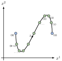
Figure 1: Formation profile of $11$ agents in the $\left(x^{1},x^{2}\right)$-plane; $\color[rgb]{0.6,0.6,0.6}\bullet$ refer to the leader agents, $\color[rgb]{0.6,0.6,0.6}\bullet$ denote the followers.

The basic idea is illustrated schematically in Fig. 1. Herein, $11$ agents in a so-called leader-follower configuration are arranged in the plane. The two types of agents refer to active and collaborative roles, however leaders may have to fulfil more sophisticated tasks than followers. By moving from the discrete set of agents denoted by coloured dots to an agent continuum the formation is visualized by the line with $z$ being interpreted as a virtual communication path. The formation is thereby obtained by the superposition of solutions of PDEs in the individual directions $x^{1}$ and $x^{2}$.

This contribution addresses the design of a two-degrees-of-freedom (2DOF) boundary control concept. The approach combines motion planning and feedforward control with stabilising tracking control for a multi-agent continuum model in terms of coupled linear, time-variant diffusion-reaction equations. It is shown that this setting allows us to recover a wide range of common multi-agent dynamics and enables us to realise various formation shapes. This extends the previous work (Freudenthaler and Meurer, 2016) of the authors in several directions: (i) a state observer for the continuum model is included into the control loop; (ii) the stability of the closed-loop control is rigorously assessed using Lyapunov’s stability theory; (iii) the decentralised distribution and synchronisation of in particular parameter values through the multi-agent network is addressed; (iv) a first experimental verification of the theoretical results is provided using a small swarm of mobile robots.

Motion planning and feedforward control design are based on the flatness property of the continuum model, which is exploited by taking into account results from Meurer and Kugi (2009b); Freudenthaler and Meurer (2016) to use the formal integration of the coupled PDEs. The continuum model is composed of two PDEs with the state of the first PDE referring to the spatial location of an agent element. The second PDE couples into the first PDE and governs the spatial-temporal distribution of its reaction parameter. By controlling this reaction parameter evolution desired parameter adaptations can be conducted, which results in a rich class of possible formation profiles. Formations herein correspond to steady state solutions of the continuum model. To address the deployment into unstable formations the flatness-based feedforward control is extended by an error state feedback to obtain a tracking controller involving a Luenberger-type state observer. The design of both the controller and the observer makes use of the backstepping technique, which has been extensively studied for different types of PDEs, see, e.g., Krstic and Smyshlyaev (2008). For diffusion-reaction equations the linear, time-invariant case is addressed, e.g., in Smyshlyaev and Krstic (2004, 2005); Baccoli et al. (2015) with extensions to the time-varying case provided, e.g., in Meurer and Kugi (2009a); Jadachowski et al. (2012); Meurer (2013). In addition to simulation studies this contribution presents first experimental results for the considered PDE-based formation control concept by using a small swarm of mobile robots. It is shown that the combined flatness- and backstepping-based tracking controller enables us to experimentally achieve transitions even into unstable formation profiles with a spatial relocation of the swarm.

The article is organized as follows: Section 2 introduces the model of the agent dynamics involving the spatial-temporal parameter evolution and defines steady state formation profiles. The 2DOF control concept is discussed in the two subsequent sections including the flatness-based feedforward control approach in Section 3 and the observer-based stabilisation of the tracking error dynamics in Section 4. The formal transfer to the discrete setup imposing the communication topology and simulations studies are provided in Section 5. The implementation at a test-rig and experimental results are presented in Section 6. Some final remarks in Section 7 conclude the paper.

2 Problem formulation

In the following a continuum formulation using PDEs is introduced to model the agent dynamics. For this the connection between the continuum model and the related ODE formulation of a multi-agent system under next-neighbor communication is addressed, which is also utilized in Sections 5.2 and 6 for the implementation in the simulation and the experimental environment.

2.1 Multi-agent system model

Taking into account the undirected line graph $G(V,E)$ of Fig. 1 with node set $V$ and edge set $E$. Nodes $j,\,k\in V$ can share information if $(i,j)\in E$, i.e., $i\sim j$. Let $(x_{j}^{1}(t),x_{j}^{2}(t))$ denote the position of agent $j$ at time $t$ in the $(x^{1},x^{2})$-plane. Let $N+1$ denote the number of nodes in $V$. Nodes $j\in V$ are numbered consecutively starting from $0$ to $N$ with $j\in\{0,N\}$ denoting leaders and $j\in\{1,N-1\}$ representing followers. The multi-agent system is considered under the (time-varying) next-neighbor protocol

$$\dot{x}_{j}^{i}(t) =\mathfrak{a}^{i}\sum_{k\sim j}\big{(}x_{k}^{i}(t)-x_{j}^{i}(t)\big{)}+c_{j}^{i}(t)x_{j}^{i}(t)$$ (1a)

$$\dot{c}_{j}^{i}(t) =\mathfrak{b}^{i}\sum_{k\sim j}\big{(}c_{k}^{i}(t)-c_{j}^{i}(t)\big{)}+d_{j}^{i}(t)c_{j}^{i}(t)$$ (1b)

for all follower agents $$j=1,2,\ldots,N-1 \mathfrak{a}^{i}>0 \mathfrak{b}^{i}>0 d_{j}^{i}(t)\in\mathbb{R} \mathfrak{a}^{i} \mathfrak{b}^{i} 1/(N+1) c_{j}^{i}(t) d_{j}^{i}=0 c_{k}^{i}(t)-c_{j}^{i}(t) k\sim j$$. The parameters satisfy , , with , in general showing some proportionality to by means of the adjacency matrix (Mesbahi and Egerstedt, 2010) or particular influence functions in opinion dynamics (Motsch and Tadmor, 2014). While (1a) describes the motion of the agents the variable , as it couples into (1a), enables us to distribute parameter information, which directly influences the agent dynamics. It is shown subsequently that this broadens the applicability of the setup in particular for motion planning and formation control. If , then this information processing requires only relative data, i.e., for . The protocol includes the graph-Laplacian control to achieve consensus (Olfati-Saber et al., 2007).

To control agent motion and parameter information external control signals are imposed at the leader agents $j\in\{0,N\}$ in terms of

$$\dot{x}_{0}^{i}(t)=u_{0}^{i}(t), \dot{x}_{N}^{i}(t)=u_{N}^{i}(t)$$ (1c)

$$\dot{c}_{0}^{i}(t)=v_{0}^{i}(t), \dot{c}_{N}^{i}(t)=v_{N}^{i}(t).$$ (1d)

At the time $t=t_{0}$ the agents are at the initial state

$$x_{j}^{i}(t_{0})=x_{j,0}^{i}, c_{j}^{i}(t_{0})=c_{j,0}^{i}.$$ (1e)

2.2 From discrete to diffusion-like continuum model

When considering a large-scale multi-agent system it is reasonable to map the discrete agent set $j\in V$ into an agent continuum defined on the continuous coordinate $z\in[0,\ell]$ representing the agent index in the continuous communication topology. In view of this, the states $x_{j}^{i}(t)$ and $c_{j}^{i}(t)$ approach $x^{i}(z,t)$ and $c^{i}(z,t)$ and the next-neighbor configuration (1) translates into the coupled diffusion-reaction system (DRS)

$$\partial_{t}x^{i}(z,t) =a^{i}\partial^{2}_{z}x^{i}(z,t)+c^{i}(z,t)x^{i}(z,t)$$ (2a)

$$\partial_{t}c^{i}(z,t) =b^{i}\partial^{2}_{z}c^{i}(z,t)+d^{i}(z,t)c^{i}(z,t)$$ (2b)

defined on the domain $$\mathcal{D}(\ell):=\{(z,t)\in(0,\ell)\times\left(t_{0},\infty\right)\}$$ with the boundary controls

$$\partial_{t}{x^{i}}(0,t) =u_{0}^{i}(t), \partial_{t}{x^{i}}(\ell,t)=u_{\ell}^{i}(t)$$ (2c)

$$\partial_{t}{c^{i}}(0,t) =v_{0}^{i}(t), \partial_{t}{c^{i}}(\ell,t)=v_{\ell}^{i}(t)$$ (2d)

and the initial conditions

$${x^{i}}(z,t_{0})={x}{{}_{0}^{i}}(z) {c^{i}}(z,t_{0})=c_{0}^{i}(z).$$ (2e)

Remark 1.

Since the problem formulation (2) is independent for each tuple $(x^{i}(z,t),c^{i}(z,t))$ the superscript $i$ referring to the coordinate axis is subsequently omitted.

The following proposition addresses a remark by Enrique Zuazua concerning collective dynamics using mean field and diffusion-like PDE approaches (Zuazua, 2018).

Proposition 2 (Discrete vs. continuum dynamics).

Consider a next-neighbor configuration on a line graph with $N+1$ nodes. Denote by $\Delta z=\ell/N$ the step size and introduce the location (agent index) $z_{j}=j\Delta z$ with $j=0,1,\ldots,N<\infty$. The discrete formulation (1) and the continuum formulation (2) can be formally exchanged at any $z_{j}$ with error $O^{4}(\Delta z)$ up to the scaling $t\mapsto r(N,\ell)t$, $c\mapsto c/r(N,\ell)$, $d\mapsto d/r(N,\ell)$ with $r(N,\ell)=(\ell^{2}\mathfrak{a})/(N^{2}a)$.

The claim is supposed to provide a principal connection and makes use of classical smooth solutions of (2) to allow for a Taylor series expansion. Assuming regularity of solutions set $c_{j}(t)=c(z_{j},t)$, $x_{j}(t)=x(z_{j},t)$ and consider the Taylor series expansion

$$x_{j\pm 1}(t) =x((j\pm 1)\Delta z,t)$$

$$=x(j\Delta z,t)\pm\partial_{z}x(j\Delta z,t)\Delta z$$

$$\phantom{=}\,+\partial^{2}_{z}x(j\Delta z,t)\frac{(\Delta z)^{2}}{2!}\pm O^{3}(\Delta z).$$

Replacing $x$ by $c$ yields the respective expansion for $c_{j\pm 1}(t)$. Substitution into (1) for a two-neighbor configuration yields

$$\partial_{t}x(z_{j},t) =\mathfrak{a}(\Delta z)^{2}\partial^{2}_{z}x(z_{j},t)+c(z_{j},t)x(z_{j},t)$$ (3a)

$$\partial_{t}c(z_{j},t) =\mathfrak{b}(\Delta z)^{2}\partial^{2}_{z}c(z_{j},t)+d(z_{j},t)c(z_{j},t)$$ (3b)

with error $O^{4}(\Delta z)$. With $\Delta z=\ell/N$ the proposed scaling in terms of $r(N,\ell)$ transfers (3) to

$$\partial_{t}x(z_{j},t) =a\partial^{2}_{z}x(z_{j},t)+c(z_{j},t)x(z_{j},t)$$ (4a)

$$\partial_{t}c(z_{j},t) =b\partial^{2}_{z}c(z_{j},t)+d(z_{j},t)c(z_{j},t)$$ (4b)

with $b={\mathfrak{b}a}/{\mathfrak{a}}$. The computation above addresses the transfer from the discrete to the continuum model, the reverse can be obtained, e.g., by a finite difference discretization of (2) or similarly the substitution of the Taylor series expansion. Comparing (4) with (2) illustrates the formal relationship. Note that alternatively $\ell$ can be adjusted for unscaled $t$. To further interpret the result let $c_{j}(t)=c(z_{j},t)=0$. In this case the discrete formulation is the graph-Laplace protocol (Olfati-Saber, 2006). Hence, as the number of nodes $N+1$ increases (thus $1/(N+1)$ decreases) all non-zero eigenvalues of the system matrix tend to zero. For $N\to\infty$ the system rests in the initial state. This is contrary to the dynamical behavior of the structurally corresponding heat equation (2) obtained for $c(z,t)=0$. Taking into account the time scaling $t\mapsto(\ell^{2}\mathfrak{a})/(N^{2}a)t$ for $N\to\infty$ reproduces the discrete case.

2.3 Formation control problem

The deployment of the multi-agent system into desired formation profiles and the finite time transition between different formation profiles is addressed by developing a combined feedforward-feedback control strategy for the leader agents (1c), (1d) in the discrete setting or (2c), (2d) in the continuum setting, respectively.

Definition 3 (Steady state).

Let $d(z,t)$ be continuous in $z$, smooth in $t$ but locally non-analytic with $d(z,t)=\bar{d}(z)$ and $\partial^{n}_{t}d(z,t)=0$ for all $n\geq 1$ at some fixed $t$. The tuple

$$(\bar{x}(z),\bar{c}(z))=(\bar{x}(z;\bar{x}_{0},\bar{x}_{\ell}),\bar{c}(z;\bar{c}_{0},\bar{c}_{\ell},\bar{d}(z))).$$ (5)

with $\bar{x}(z),\,\bar{c}(z)\in C^{2}([0,\ell])$ is a steady state of (2) if

$$a\partial^{2}_{z}\bar{x}(z)+\bar{c}(z)\bar{x}(z)=0,~{}b\partial^{2}_{z}\bar{c}(z)+\bar{d}(z)\bar{c}(z)=0$$ (6a)

for $$z\in(0,\ell)$$ and

$$\bar{x}(0)=\bar{x}_{0},\quad\bar{x}(\ell)=\bar{x}_{\ell},\quad\bar{c}(0)=\bar{c}_{0},\quad\bar{c}(\ell)=\bar{c}_{\ell}$$ (6b)

hold true for some $$\bar{x}_{0},\,\bar{x}_{\ell},\,\bar{c}_{0},\,\bar{c}_{\ell}\in\mathbb{R}$$.

The constant boundary values $\bar{x}_{\mathrm{0}}$, $\bar{x}_{\mathrm{\ell}}$, $\bar{c}_{\mathrm{0}}$, and $\bar{c}_{\mathrm{\ell}}$ can be freely assigned since under steady state conditions (2c), (2d) reduce to $u_{0}(t)=u_{\ell}(t)=v_{0}(t)=v_{\ell}(t)=0$.

Remark 4.

For the sake of simplicity no distinction between different boundary values $\bar{x}_{\mathrm{0}}$, $\bar{x}_{\mathrm{\ell}}$, $\bar{c}_{\mathrm{0}}$, and $\bar{c}_{\mathrm{\ell}}$ is made. This is, of course, implicitly included.

Definition 5 (Set of steady states).

Let $d(z,t)$ be continuous in $z$, smooth in $t$ but locally non-analytic at discrete time instances $t_{j}$, $1\leq j<\infty$ with $0\leq t_{0}$, $t_{j-1}<t_{j}$ so that $d(z,t_{j})=\bar{d}_{t_{j}}(z)$ and $\partial^{n}_{t}d(z,t)|_{t=t_{j}}=0$ for all $n\geq 1$. The set of steady states endowed with the $C^{2}$ topology is denoted by $\mathcal{S}=\bigcup_{j}\{(\bar{x}_{t_{j}}(z),\bar{c}_{t_{j}}(z))\}$ with the tuple $(\bar{x}_{t_{j}}(z),\bar{c}_{t_{j}}(z))$ solving (6) for $\bar{d}(z)=\bar{d}_{t_{j}}(z)$.

With these preparations the considered type of formation profiles and spatial-temporal formation transitions can be properly introduced:

1. Formation profiles denoted by the tuple $(\bar{x}^{\ast}(z),\bar{c}^{\ast}(z))$ are steady states according to Definition 3 so that

   $$\bar{x}^{\ast}(z)\!=\!\bar{x}(z;\bar{x}^{\ast}_{0},\bar{x}^{\ast}_{\ell}),~{}\bar{c}^{\ast}(z)\!=\!\bar{c}(z;\bar{c}^{\ast}_{0},\bar{c}^{\ast}_{\ell},\bar{d}^{\ast}(z)).$$ (7)

2. Denote by $(\bar{x}^{\ast}_{t_{j-1}}(z),\bar{c}^{\ast}_{t_{j-1}}(z))$ and $(\bar{x}^{\ast}_{t_{j}}(z),\bar{c}^{\ast}_{t_{j}}(z))$ two different formation profiles belonging to the same connected component of $\mathcal{S}$. The transition from $(\bar{x}^{\ast}_{t_{j-1}}(z),\bar{c}^{\ast}_{t_{j-1}}(z))$ to $(\bar{x}^{\ast}_{t_{j}}(z),\bar{c}^{\ast}_{t_{j}}(z))$ in the finite time interval $t\in[t_{j-1},t_{j}]$ is achieved, if inputs $u_{0}(t)$, $u_{\ell}(t)$, $v_{0}(t)$, $v_{\ell}(t)$ exist for $t\in[t_{j-1},t_{j}]$ so that starting from $(x(z,t_{j-1}),c(z,t_{j-1}))=(\bar{x}^{\ast}_{t_{j-1}}(z),\bar{c}^{\ast}_{t_{j-1}}(z))$ the solution $(x(z,t_{j}),c(z,t_{j}))=(\bar{x}^{\ast}_{t_{j}}(z),\bar{c}^{\ast}_{t_{j}}(z))$ is obtained.

Remark 6.

The inclusion of the second state $c(z,t)$ into the problem formulation extends the possible set of formation profiles. To illustrate this consider the computation of the steady state (only $\bar{c}$-contribution) according to (6) for (i) $\bar{d}_{0}(z)=0$, i.e., $\bar{c}(z)=\bar{c}_{0}+z(\bar{c}_{\ell}-\bar{c}_{0})$ and (ii) $\bar{d}_{0}(z)=\pi^{2}$, $\bar{c}_{0}=\bar{c}_{\ell}=0$, i.e., $\bar{c}(z)=k\sin(\pi z)$, $k\neq 0$. Since there are obviously smooth functions $d(z,t)$ with $d(z,t_{0})=0$, $d(z,t_{1})=\pi^{2}$ for some $t_{1}>t_{0}$, locally non-analytic at $t\in\{t_{0},t_{1}\}$ this example confirms that the $c$-dynamics can be controlled by $d(z,t)$ and the boundary inputs $v_{0}(t)$ and $v_{\ell}(t)$ to connect different families of steady states. The explicit constructive solution of this trajectory planning problem is presented in Section 3.

While in general a numerical solution of (6) is required, analytic expressions can be determined for special cases. For $\bar{d}(z)=0$ (6) yields

$$\begin{split}&a\partial^{2}_{z}\bar{x}(z)+\Big{(}\bar{c}_{0}+(\bar{c}_{\ell}-\bar{c}_{0})\frac{z}{\ell}\Big{)}\bar{x}(z)=0,\quad z\in(0,\ell)\\ &\bar{x}(0)=\bar{x}_{0},~{}\bar{x}(\ell)=\bar{x}_{\ell},\end{split}$$ (8)

whose solution, without imposing additional conditions on the coefficients, can be determined by means of Airy functions. Let in addition $\bar{c}_{0}=\bar{c}_{\ell}$, then steady state formation profiles $\bar{x}(z)$ can be written as

$$\bar{x}(z)=k_{1}\exp{(s_{1}z)}+k_{2}\exp{(s_{2}z)}\,.$$ (9)

For $a>0$ three scenarios are possible: (i) If $\bar{c}_{0}<0$, then the solution is (9) with $\{s_{1},s_{2},k_{1},k_{2}\}\in\mathbb{R}$; (ii) if $\bar{c}_{0}>0$, then the solution reads

$$\bar{x}(z)=k^{\prime}\cos{(\theta z)}+k^{\prime\prime}\sin{(\theta z)}\,\quad k^{\prime},~{}k^{\prime\prime}\in\mathbb{R};$$ (10)

and (iii) if $\bar{c}_{0}=0$ one obtains $\bar{x}(z)=k_{1}+k_{2}z$. The explicit computation of the coefficients $k_{1}$ and $k_{2}$ relies on the values $\bar{x}_{0}$ and $\bar{x}_{\ell}$ of the leader agents in (6). Particular examples are shown in Fig. 2 when solving the boundary value problem as described before individually for the $x^{1}$- and the $x^{2}$-direction given the parameters of Tab. 1. In general the overlay of solutions (9) in the two dimensional plane generates shapes of the well-known Lissajous curves. Note that for the circle formation the parameter configuration for the $x^{2}$-coordinate allows an arbitrary setting for $k^{\prime\prime}$ but with $k^{\prime}=0$ in (10). Consequently, the steady state solution is not uniquely determined but can be freely scaled in $k^{\prime\prime}$.

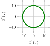
(a) Circle formation

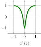
(b) Gull-like formation

Figure 2: Formation profiles from the overlay of solutions to (6) for parameter values according to Tab. 1.

Table 1: Parameters for the formation profiles in Fig. 2.

Profile	Coord.	$a$	$\bar{c}_{0},\,\bar{c}_{\ell}$	$\bar{x}_{0}$	$\bar{x}_{\ell}$
circle	$x^{1}:$	$1$	$(2\pi/\ell)^{2}$	$10$	$10$
	$x^{2}:$	$1$	$(2\pi/\ell)^{2}$	$0$	$0$
gull-like	$x^{1}:$	$1$	$-(7/\ell)^{2}$	$-1$	$1$
	$x^{2}:$	$1$	$(2\pi/\ell)^{2}$	$1$	$1$

3 Trajectory planning for agent continuum

Trajectory planning refers to the determination of the input trajectories so that the system state or output follows a certain predefined path. This problem is subsequently solved by exploiting the flatness property of multi-agent continuum model (2).

3.1 Formal state and input parametrisation

To differentially parametrise the system state ${\boldsymbol{\eta}}(z,t)=[x(z,t),c(z,t)]^{T}$ and the boundary controls ${\boldsymbol{\kappa}}_{0}(t)=[u_{0}(t),v_{0}(t)]^{T}$ at $z=0$ and ${\boldsymbol{\kappa}}_{\ell}(t)=[u_{\ell}(t),v_{\ell}(t)]^{T}$ at $z=\ell$ formal integration as proposed in Meurer and Kugi (2009b); Meurer (2013) is extended to the multi-input case with inputs on opposite boundaries of the domain. Let

$${\boldsymbol{f}}({\boldsymbol{\eta}},z,t)=\begin{bmatrix}\frac{1}{a}\big{(}\partial_{t}x(z,t)-c(z,t)x(z,t)\big{)}\\ \frac{1}{b}\big{(}\partial_{t}c(z,t)-d(z,t)c(z,t)\big{)}\end{bmatrix}$$

and solve (2a), (2b) for $[\partial^{2}_{z}x(z,t),\partial^{2}_{z}c(z,t)]^{T}$. Integrating the resulting expression twice in $z$ yields

$${\boldsymbol{\eta}}(z,t)={\boldsymbol{\eta}}(\xi,t)+(z-\xi)\partial_{z}{\boldsymbol{\eta}}(z,t)|_{z=\xi}\\ +\int^{z}_{\xi}\int^{\chi}_{\xi}{\boldsymbol{f}}({\boldsymbol{\eta}},\sigma,t)\mathrm{d}\sigma\mathrm{d}\chi.$$ (11)

for arbitrary but fixed $\xi\in[0,\ell]$. As a result

$${\boldsymbol{y}}_{1}(t)={\boldsymbol{\eta}}(\xi,t),\quad{\boldsymbol{y}}_{2}(t)=\partial_{z}{\boldsymbol{\eta}}(z,t)|_{z=\xi}$$ (12)

serve as degrees-of-freedom. This enables us to implicitly express ${\boldsymbol{\eta}}(z,t)$ and thus the boundary inputs $({\boldsymbol{\kappa}}_{0}(t),{\boldsymbol{\kappa}}_{\ell}(t))$ in terms of $({\boldsymbol{y}}_{1}(t),{\boldsymbol{y}}_{2}(t))$ according to

$${\boldsymbol{\eta}}(z,t) ={\boldsymbol{y}}_{1}(t)+(z-\xi){\boldsymbol{y}}_{2}(t)$$

$$\phantom{=}+\int^{z}_{\xi}\int^{\chi}_{\xi}{\boldsymbol{f}}({\boldsymbol{\eta}},\sigma,t)\mathrm{d}\sigma\mathrm{d}\chi$$ (13a)

$${\boldsymbol{\kappa}}_{0}(t) =\partial_{t}{\boldsymbol{\eta}}(0,t),~{}{\boldsymbol{\kappa}}_{\ell}(t)=\partial_{t}{\boldsymbol{\eta}}(\ell,t)$$ (13b)

An explicit expression can be obtained either by iteration or successive approximation. For the latter consider the functional series

$${\boldsymbol{\eta}}(z,t)=\sum_{n=0}^{\infty}{\boldsymbol{\eta}}_{n}(z,t),$$ (14)

whose substitution into (13a) motivates the computational rule

$$\begin{split}{\boldsymbol{\eta}}_{0}(z,t)&={\boldsymbol{y}}_{1}(t)+(z-\xi){\boldsymbol{y}}_{2}(t)\\ {\boldsymbol{\eta}}_{n}(z,t)&=\int^{z}_{\xi}\int_{\xi}^{\chi}{\boldsymbol{f}}({\boldsymbol{\eta}}_{n-1},\sigma,t)\mathrm{d}\sigma\mathrm{d}\chi,\quad n\geq 1.\end{split}$$ (15)

In other words $({\boldsymbol{y}}_{1}(t),{\boldsymbol{y}}_{2}(t))$ defined in (12) for arbitrary $\xi\in[0,\ell]$ can be considered a flat output for the multi-agent continuum model (2). The explicit evaluation of (14), (15) thereby relies on the convergence of the obtained expressions, which, as is shown below, reduces to a problem of trajectory assignment for the flat output.

3.2 Convergence analysis

For the convergence analysis the notion of a Gevrey class function is required (Rodino, 1993).

Definition 7 (Gevrey class functions).

The function $y(t)$ is in $G_{\alpha}^{D}(\mathbb{R})$, the Gevrey class of order $\alpha$, if $y\in C^{\infty}(\mathbb{R})$ and $\exists D\in(0,\infty)$ so that $\sup_{t\in\mathbb{R}}\left|\partial^{k}_{t}y(t)\right|\leq D^{k+1}(k!)^{\alpha}$ holds true for all $k\in\mathbb{N}\cup\{0\}$.

Definition 8.

Let $G_{\alpha}^{D}(\mathbb{R};X)$ denote the class of $X$-valued Gevrey class functions $G_{\alpha}^{D}(\mathbb{R})$ of order $\alpha$ and let $\Omega_{1}\subset\mathbb{R}$, $\Omega_{2}\subset\mathbb{R}$. By $CG^{k,\alpha}(\Omega_{1},\Omega_{2};\mathbb{R})$ we denote the class of functions $f:\Omega_{1}\times\Omega_{2}\to\mathbb{R}$ such that $f(\cdot,t)\in C^{k}(\Omega_{1};\mathbb{R})$ for every fixed $t\in\Omega_{2}$ and $f(z,\cdot)\in G_{\alpha}^{D}(\Omega_{2};\mathbb{R})$ for every fixed $z\in\Omega_{1}$.

The main convergence result reads as follows.

Theorem 9.

Let $d\in CG^{0,\alpha}([0,\ell],\mathbb{R};\mathbb{R})$ and let ${\boldsymbol{y}}_{1},\,{\boldsymbol{y}}_{2}\in(G_{\alpha}^{D}(\mathbb{R}))^{2}$ with $\alpha\leq 2$. Then ${\boldsymbol{\eta}}(z,t)$ determined from the series (14) with coefficients (15) fulfills ${\boldsymbol{\eta}}\in(CG^{2,\alpha}([0,\ell],\mathbb{R};\mathbb{R}))^{2}$ and the series (14) converges absolutely and uniformly for all $z\in[0,\ell]$ if $\alpha\in[1,2)$.

The proof of this result follows in principle from the analysis in Meurer and Kugi (2009b) but with the modification that the flat output is located at some fixed but arbitrary in-domain position $\xi\in[0,\ell]$. For the convergence analysis the cascaded structure of the PDEs (2) is exploited by first analyzing the differential parametrization of $\eta_{2}(z,t)=c(z,t)$. Taking into account the assumptions on ${\boldsymbol{y}}_{1}(t)$, ${\boldsymbol{y}}_{2}(t)$ and $d(z,t)$ and the recursion (15) it can be rather straightforwardly verified by induction that the $\mathbb{N}\cup\{0\}\ni l$-th time derivative of $\eta_{2,n}(z,t)=c_{n}(z,t)$ fulfills

$$\sup_{t\in\mathbb{R}}|\partial_{t}^{l}c_{n}(z,t)|\leq D^{l+n+1}(l+n)!^{\alpha}M_{n}g_{n}(z,\xi)$$ (16)

with $M_{n}=\frac{1}{b^{n}}\prod_{j=1}^{n}(1+\frac{1}{j^{\alpha}})$, $M_{0}=1$ and $g_{n}(z,\xi)={|z-\xi|^{2n}}/{(2n)!}+{|z-\xi|^{2n+1}}/{(2n+1)!}$. Observing $b^{n}M_{n}=\prod_{j=1}^{n}(1+j^{\alpha})/\prod_{j=1}^{n}j^{\alpha}\leq(n+1)^{\alpha}$ the estimate (16) for $l=0$ implies

$$\sup_{t\in\mathbb{R}}|c_{n}(z,t)| \leq D^{n+1}(n)!^{\alpha}M_{n}g_{n}(z,\xi)$$

$$\leq D\bigg{(}\frac{D}{b}\bigg{)}^{n}(n+1)!^{\alpha}g_{n}(z,\xi)$$

In view of (14) and $g_{n}(z,\xi)=|z-\xi|^{2n}/(2n)!\times(1+|z-\xi|)/(2n+1))\leq(1+\ell)(z-\xi)^{2n}/(2n)!$ this yields the upper power series estimate on the functional series

$$|c(z,t)| \leq D\sum_{n=0}^{\infty}\bigg{(}\frac{D}{b}\bigg{)}^{n}(n+1)!^{\alpha}g_{n}(z,\xi)$$

$$\leq D(1+\ell)\sum_{n=0}^{\infty}\frac{(n+1)!^{\alpha}}{(2n)!}\kappa^{n}=\sum_{n=0}^{\infty}\beta_{n}\kappa^{n}$$

with $\kappa=D|z-\xi|^{2}/b$. Absolute and uniform convergence with infinite radius of convergence for $\alpha\in[1,2)$ hence follows from the Cauchy-Hadamard theorem applied to the coefficient $\beta_{n}$.

By proceeding similarly with $c_{n}(z,t)$ replaced by $\partial_{t}^{l}c_{n}(z,t)$ and the construction in terms of formal integration it can be deduced that $c(z,t)$ obtained from (14), (15) fulfills $c\in CG^{2,\alpha}([0,\ell],\mathbb{R};\mathbb{R})$. This result directly implies that the convergence analysis for $\eta_{1}(z,t)=x(z,t)$ follows exactly the lines above for $c(z,t)$, which proves the claim. ∎

3.3 Trajectory assignment

Based on the flatness analysis above desired trajectories for the flat outputs ${\boldsymbol{y}}_{1}(t)$ and ${\boldsymbol{y}}_{2}(t)$ can be assigned independently to achieve prescribed finite time transitions between formation profiles. According to Section 2.3 these are completely determined by solving the boundary-value problem (6). Let $(\bar{x}_{0}^{\ast},\bar{x}_{\ell}^{\ast})$ and $(\bar{c}_{0}^{\ast},\bar{c}_{\ell}^{\ast})$ denote the desired boundary values (6b) of the formation $(\bar{x}^{\ast}(z),\bar{c}^{\ast}(z))$. With (7) and (12) the resulting formation profile can be translated into steady state values of the flat outputs according to

$${\boldsymbol{y}}_{1}^{\ast}=\begin{bmatrix}\bar{x}^{\ast}(\xi;\bar{x}_{0}^{\ast},\bar{x}_{\ell}^{\ast})\\ \bar{c}^{\ast}(\xi;\bar{c}_{0}^{\ast},\bar{c}_{\ell}^{\ast})\end{bmatrix},\quad{\boldsymbol{y}}_{2}^{\ast}=\begin{bmatrix}\partial_{z}\bar{x}^{\ast}(\xi;\bar{x}_{0}^{\ast},\bar{x}_{\ell}^{\ast})\\ \partial_{z}\bar{c}^{\ast}(\xi;\bar{c}_{0}^{\ast},\bar{c}_{\ell}^{\ast})\end{bmatrix}.$$ (17)

By changing $(\bar{x}_{0}^{\ast},\bar{x}_{\ell}^{\ast})$ and $(\bar{c}_{0}^{\ast},\bar{c}_{\ell}^{\ast})$ different formation profiles are obtained, which can be connected by properly assigning the temporal transition path for the flat output. To illustrate this let ${\boldsymbol{y}}_{1,0}^{\ast}$, ${\boldsymbol{y}}_{2,0}^{\ast}$ and ${\boldsymbol{y}}_{1,\tau}^{\ast}$, ${\boldsymbol{y}}_{2,\tau}^{\ast}$ denote steady state values determined from (17) corresponding to two formation profiles $(\bar{x}^{\ast}_{t_{0}}(z),\bar{c}^{\ast}_{t_{0}}(z))$ and $(\bar{x}^{\ast}_{t_{1}}(z),\bar{c}^{\ast}_{t_{1}}(z))$ to be attained at times $t=t_{0}$ and $t=t_{1}=t_{0}+\tau$, respectively. The transition between these two profiles within the finite time interval $t\in[t_{0},t_{0}+\tau]$ can be realized by assigning

$${{\boldsymbol{y}}}^{\ast}_{j}(t) ={\boldsymbol{y}}_{j,0}^{\ast}+\big{(}{\boldsymbol{y}}_{j,\tau}^{\ast}-{\boldsymbol{y}}_{j,0}^{\ast}\big{)}\Phi_{\tau}(t-t_{0})$$ (18)

for $j\in\{1,2\}$. Herein, $\Phi_{\tau}(\cdot)$ has to be a Gevrey class function according to Def. 7 being locally non-analytic at $t=t_{0}$ and $t=t_{0}+\tau$, i.e., $\Phi_{\tau}(0)=0$, $\Phi_{\tau}(\tau)=1$ with $\partial_{t}^{l}\Phi_{\tau}|_{t\in\{0,\tau\}}=0$ for $l\in\mathbb{N}$. The latter requires a Gevrey order $\alpha>1$ with $\alpha<2$ being imposed from Thm. 9. Examples for functions $\Phi_{\tau}(\cdot)$ are provided, e.g., in Rodino (1993); Laroche et al. (2000).

Moreover, given an arbitrary formation profile $\bar{x}^{d}(z)$, which does not fulfill (6) the presented approach can be extended to approximately obtain the desired profile. For this, the static optimization problem is formulated

$$\begin{split}&\min_{\bar{c}_{0},\bar{c}_{\ell},\bar{d}(z)}J\big{[}\bar{x}(z)-\bar{x}^{d}(z)\big{]}\\ &\text{s.t.}~{}\bar{x}(z)~{}\text{fulfills \eqref{eq:sec2:problemStdyst} for}~{}\bar{x}_{0}=\bar{x}^{d}(0),\,\bar{x}_{\ell}=\bar{x}^{d}(\ell).\end{split}$$ (19)

Herein, $J[\cdot]$ is a positive definite functional to be chosen suitably depending on the problem to minimize the difference between the steady state $\bar{x}(z)$ and the desired formation profile $\bar{x}^{d}(z)$.

3.4 Feedforward control

Given the desired flat output trajectories the corresponding feedforward control signals follow from (13b) with ${\boldsymbol{\eta}}(z,t)$ replaced by ${\boldsymbol{\eta}}^{\ast}(z,t)$ computed in terms of the series (14) with recursively evaluated coefficients (15) in terms of ${\boldsymbol{y}}_{1}^{\ast}(t)$, ${\boldsymbol{y}}_{2}^{\ast}(t)$. This yields

$${\boldsymbol{\kappa}}_{0}^{\ast}(t)=\partial_{t}{\boldsymbol{\eta}}^{\ast}(0,t),\quad{\boldsymbol{\kappa}}_{\ell}^{\ast}(t)=\partial_{t}{\boldsymbol{\eta}}^{\ast}(\ell,t).$$ (20)

4 Observer-based tracking control

Since formation profiles may correspond also to unstable steady states of the PDE a stabilizing feedback control is required. In view of motion planning and the resulting feedforward control subsequently the spatial-temporal tracking error is stabilized using a backstepping approach involving a distributed parameter state observer. This results in a so-called two-degrees-of-freedom (2DOF) control approach with the desired motion induced by the feedforward control and the stabilization provided by the feedback control.

4.1 Stabilisation of tracking error dynamics

The state $c(z,t)$ is used to distribute information to the PDEs (2a) governing the agent position $x(z,t)$.

Assumption 10.

The solution to (2b), (2d) with initial state (2e) fulfills $c^{i}(z,t)\in CG^{2,\alpha}([0,\ell],\mathbb{R};\mathbb{R})$, $\alpha\leq 2$.

This assumption can be fulfilled in a straightforward way by a proper choice of $d^{i}(z,t)$, see also the main convergence result in Theorem 9, and implies that $c^{i}(z,t)$ is bounded. In view of Assumption 10 and the cascaded structure consisting of (2a) and (2b) the sub-dynamics for $c(z,t)$ is subsequently assumed to be only controlled by the feedforward control $(v_{0}^{\ast}(t),v_{\ell}^{\ast}(t))$. To emphasize this fact $c^{\ast}(z,t)$ is written subsequently when referring to this solution. Contrary the sub-dynamics for $x(z,t)$ is controlled using a combined feedforward-feedback strategy. Since flatness-based motion planning by construction fulfills the PDE (2a) with $(x(z,t),u_{0}(t),u_{\ell}(t))$ replaced by $({x}^{\ast}(z,t),{u}^{\ast}_{0}(t),{u}^{\ast}_{\ell}(t))$ the tracking error dynamics in the error state $e(z,t)=x(z,t)-{x}^{\ast}(z,t)$ reads

$$\begin{split}\partial_{t}e(z,t)&=a\partial^{2}_{z}e(z,t)+c^{\ast}(z,t)e(z,t)\\ \partial_{t}{e}(0,t)&=u_{0}(t)-{u}^{\ast}_{0}(t)=\Delta u_{0}(t)\\ \partial_{t}{e}(\ell,t)&=u_{\ell}(t)-{u}^{\ast}_{\ell}(t)=\Delta u_{\ell}(t).\end{split}$$ (21)

Herein, $\Delta u_{0}(t)$ and $\Delta u_{\ell}(t)$ are used to establish state feedback control. For this backstepping is used by introducing the invertible time-varying Volterra integral transformation

$$\mathfrak{v}(z,t)=e(z,t)-\int_{0}^{z}{k(z,s,t)e(s,t)}\,\mathrm{d}{s},$$ (22)

with the integral kernel $k(z,s,t)$ defined on $(z,s,t)\in\mathcal{T}_{k}(\ell):=\left\{(z,s,t)\in\mathbb{R}^{2}\times\mathbb{R}_{t_{0}}^{+}\mid s\in[0,\ell],z\in\left[s,\ell\right]\right\}$ to invertibly map (21) into the target system

$$\begin{split}\partial_{t}\mathfrak{v}(z,t)&=a\partial^{2}_{z}\mathfrak{v}(z,t)-\mu(t)\mathfrak{v}(z,t)\\ &\phantom{=}\,-a\partial_{s}k(z,0,t)\mathfrak{v}(0,t),~{}z\in(0,\ell),\,t>t_{0}\\ \partial_{t}\mathfrak{v}(0,t)&=-\mu(t)\mathfrak{v}(0,t)~{}\partial_{t}\mathfrak{v}(\ell_{\mathrm{}},t)=-\mu(t)\mathfrak{v}(\ell_{\mathrm{}},t)\\ \mathfrak{v}(z,t_{0})&=\mathfrak{v}_{0}(z),~{}z\in[0,\ell].\end{split}$$ (23)

with the time-varying design parameter $\mu(t)$, see also Frihauf and Krstic (2011) for a related but time-invariant case. Differentiating (22) once with respect to $t$ and twice with respect to $z$ followed by the substitution of (23) leads, after some interim but straightforward calculations (see, e.g., Meurer (2013)), to the well-known kernel equations

$$\begin{split}\partial_{t}k(z,s,t)&=a\partial^{2}_{z}k(z,s,t)-a\partial^{2}_{s}k(z,s,t)\\ &\qquad-(c^{\ast}(s,t)+\mu(t))k(z,s,t)\\ k(z,z,t)&=-\frac{1}{2a}\int_{0}^{z}{\left\{c^{\ast}(s,t)+\mu(t)\right\}}\,\mathrm{d}{s}\\ k(z,0,t)&=0.\end{split}$$ (24)

For the determination of the solution $k(z,s,t)$ of (24) using either formal integration and successive approximation or a suitable numerical scheme the reader is referred to, e.g., Meurer and Kugi (2009a); Jadachowski et al. (2012). With Assumption 10 it can be shown that $k(z,s,t)$ is a strong solution to (24) with $k\in CG^{2,\alpha}(\Gamma,\mathbb{R};\mathbb{R})$, $\Gamma=\{(z,s)\in\mathbb{R}^{2}\mid s\in[0,\ell],z\in[s,\ell]\}$ (Vazquez et al., 2008; Meurer and Kugi, 2009a).

The state feedback controllers $\Delta u_{0}(t)$ and $\Delta u_{\ell}(t)$ follow by evaluating (22) and its time derivative at the boundaries together with (21) and (23). With this, the controller at $z=0$ reads

$$\Delta u_{0}(t)=-\mu(t)e(0,t).$$ (25a)

The evaluation at $$z=\ell$$ yields a more complex expression

$$\begin{split}\Delta u_{\ell}(t)&=-\left[\mu(t)+a\partial_{s}k(\ell,\ell,t)\right]e(\ell_{\mathrm{}},t)\\ +&\int_{0}^{\ell}{\!\!\!\!k_{I}(\ell,s,t)e(s,t)}\,\mathrm{d}{s}+ak(\ell,\ell,t)\partial_{z}e(\ell_{\mathrm{}},t)\\ +&\,a\partial_{s}k(\ell,0,t)e(0,t)\end{split}$$ (25b)

with $k_{I}(\ell,s,t)=\left[\mu(t)+c(s,t)\right]k(\ell,s,t)+\partial_{t}k(\ell,s,t)+\alpha\partial^{2}_{s}k(\ell,s,t)$. This expression results from the evaluation of the boundary condition for $z=\ell$ in (23) taking into account (21), (22) and using partial integration twice. The existence of the derivatives $\partial_{t}k(\ell,s,t)$, $\partial_{s}k(\ell,s,t)$ and $\partial^{2}_{s}k(\ell,s,t)$ in (25b) follows from $k(z,s,t)$ being a strong solution having Gevrey properties in $t$.

4.2 Closed-loop stability analysis

Subsequently well-posedness and stability of the target dynamics (23) are analysed by considering the governing equations in the space $X=H^{1}(0,\ell)$ equipped with the norm $\|h\|_{X}=\sqrt{\langle h,h\rangle_{X}}$ induced by the inner product $\langle h_{1},h_{2}\rangle_{X}=h_{1}(0)h_{2}(0)+h_{1}(\ell)h_{2}(\ell)+\langle\partial_{z}h_{1},\partial_{z}h_{2}\rangle_{L^{2}}$ for $h,\,h_{1},\,h_{2}\in X$. It is also referred, e.g., to Liang et al. (2003) for a general Banach space analysis in the non-autonomous case.

By (i) introducing the transformation $\mathfrak{v}(z,t)=\exp(-\int_{t_{0}}^{t}\mu(\tau)\mathrm{d}\tau)\mathfrak{y}(z,t)$ to remove the terms involving $\mu(t)$ from (23) followed by (ii) homogenizing the boundary conditions using $\mathfrak{x}(z,t)=\mathfrak{y}(z,t)+b_{0}(z)\mathfrak{v}_{0}(0)+b_{\ell}(z)\mathfrak{v}_{0}(\ell)$ with $b_{0}(z)=z/\ell-1$, $b_{\ell}(z)=-z/\ell$ one obtains $\partial_{t}\mathfrak{x}(z,t)=a\partial^{2}_{z}\mathfrak{x}(z,t)-a\partial_{s}k(z,0,t)\mathfrak{v}_{0}(0),~{}z\in(0,\ell),~{}t>t_{0}$ subject to $\mathfrak{x}(0,t)=\mathfrak{x}(\ell,t)=0$, $\mathfrak{x}(z,t_{0})=\mathfrak{x}_{0}(z)=\mathfrak{v}_{0}(z)+b_{0}(z)\mathfrak{v}_{0}(0)+b_{\ell}(z)\mathfrak{v}_{0}(\ell)$. The solution of the resulting inhomogeneous PDE can be determined using separation of variables and Fourier expansion. After reverting steps (ii) and (i) this yields the solution

$$\mathfrak{v}(z,t)=e^{-\int_{t_{0}}^{t}\mu(\tau)\mathrm{d}\tau}\bigg{(}S(t)\mathfrak{v}_{0}(z)-b_{0}(z)\mathfrak{v}_{0}(0)\\ -b_{\ell}(z)\mathfrak{v}_{0}(\ell)-\int_{t_{0}}^{t}S(t-\tau)a\partial_{s}k(z,0,t)\mathfrak{v}_{0}(0)\mathrm{d}\tau\bigg{)},$$

where

$$S(t)h=\sum_{k=1}^{\infty}e^{\lambda_{k}(t-t_{0})}\langle h,\phi_{k}(z)\rangle_{X}\phi_{k}(z),\quad h\in X$$

with $\lambda_{k}=-a(k\pi/\ell)^{2}$, $\phi_{k}(z)=A_{k}\sin(k\pi z/\ell)$, $A_{k}=\sqrt{2\ell}/(k\pi)$ for $k\in\mathbb{N}$ is a $C_{0}$-semigroup on $X$. By applying the Gram-Schmidt orthogonalisation procedure the functions $\phi_{-1}(z)={1}/{\sqrt{2}}$, $\phi_{0}(z)=({z}/{\ell}-{1}/{2})/\sqrt{{1}/{\ell}+{1}/{2}}$ can be determined from $b_{0}(z)$, $b_{\ell}(z)$ so that $\mathcal{B}=\{\phi_{-1}(z),\phi_{0}(z),\phi_{1}(z),\phi_{2}(z),\ldots,\phi_{k}(z),\ldots\}$ is an orthonormal set, i.e., $\langle\phi_{i},\phi_{j}\rangle_{X}=\delta_{i,j}$ for $i,j\in\mathbb{N}\cup\{-1,0\}$. Since $b_{0}(z)=-{1}/{\sqrt{2}}\phi_{-1}(z)+\sqrt{{1}/{\ell}+{1}/{2}}\phi_{0}(z)$ and $b_{\ell}(z)=-{1}/{\sqrt{2}}\phi_{-1}(z)-\sqrt{{1}/{\ell}+{1}/{2}}\phi_{0}(z)$ it follows that $\langle b_{j}(z),\phi_{k}(z)\rangle_{X}=0~{}\forall k\in\mathbb{N}$, $j\in\{0,\ell\}$, which is used to simplify $S(t)\mathfrak{x}_{0}(z)$ when solving for $\mathfrak{v}(z,t)$. Moreover it can be shown that $\langle h,\phi_{j}\rangle_{X}=0$, $j\in\mathbb{N}\cup\{-1,0\}$ implies $h=0$. Hence $\mathcal{B}$ is maximal and as a consequence is a complete orthonormal basis of $X$, see, e.g. (Kubrusly, 2011, Prop. 5.36, 5.38). For the homogeneous problem with $a\partial_{s}k(z,0,t)=0$ the orthonormality property enables us to show in a straightforward way that $\|\mathfrak{v}\|_{X}\leq\exp(-\int_{t_{0}}^{t}\mu(\tau)\mathrm{d}\tau)\|\mathfrak{v}_{0}\|_{X}$. This confirms the continuous dependence of the solution on the initial state and hence well-posedness in the sense of Hadamard. Depending on the regularity of the inhomogeneity $\partial_{s}k(z,0,t)$ classical or mild solutions can be defined. In fact $\partial_{s}k(z,s,t)\in CG^{1,\alpha}(\Gamma,\mathbb{R};\mathbb{R})$ so that for any $\mathfrak{v}_{0}\in X$ one has $\mathfrak{v}\in C([t_{0},\infty);X)\cap C^{1}((t_{0},\infty);X)$ with $\mathfrak{v}(z,t)$ fulfilling (23) pointwise. Furthermore the analysis supports the following stability result, which generalizes the approach in Frihauf and Krstic (2011) to the considered time-varying setup.

Lemma 11.

Let $0<\epsilon^{-}<\mu(t)\leq\epsilon^{+}<\infty$ for all $t\geq t_{0}$. Then the zero equilibrium of the target dynamics (23) is exponentially stable in the norm $\|\cdot\|_{X}$, i.e., there exists $M>0$ so that the inequality holds true

$$\|\mathfrak{v}\|_{X}(t)\leq Me^{-\frac{1}{2}\int_{t_{0}}^{t}\mu(s)\mathrm{d}s}\|\mathfrak{v}\|_{X}(t_{0})\\ \leq Me^{-\frac{\epsilon^{-}}{2}(t-t_{0})}\|\mathfrak{v}\|(t_{0}).$$ (26)

Consider the Lyapunov functional

$$V(t)=\frac{1}{2}\big{[}p\mathfrak{v}^{2}(0,t)+\mathfrak{v}^{2}(\ell,t)\!+\!\|\partial_{z}\mathfrak{v}\|^{2}_{L^{2}}(t)\big{]}$$ (27)

with $p\geq 0$ to be determined below. There exist positive constants $0<\beta^{-}<\beta^{+}$ so that

$$\beta^{-}\|\mathfrak{v}\|_{X}^{2}(t)\leq V(t)\leq\beta^{+}\|\mathfrak{v}\|_{X}^{2}(t).$$ (28)

A possible choice is $\beta^{-}=\min\{1/2,p/2\}$ and $\beta^{+}=\max\{1,p/2\}$. The rate of change of $V(t)$ along a solution of (23) results in

$$\partial_{t}V =p\mathfrak{v}(0)\partial_{t}\mathfrak{v}(0)+\mathfrak{v}(\ell)\partial_{t}\mathfrak{v}(\ell)+\int_{0}^{\ell}\partial_{t}\partial_{z}\mathfrak{v}\partial_{z}\mathfrak{v}\mathrm{d}z.$$

Interchanging $\partial_{t}\partial_{z}\mathfrak{v}=\partial_{z}\partial_{t}\mathfrak{v}$, integrating by parts and substituting (23) using $f(z,t):=a\partial_{s}k(z,0,t)$ gives

$$\partial_{t}V= \int_{0}^{\ell}\partial^{2}_{z}\mathfrak{v}\big{[}a\partial^{2}_{z}\mathfrak{v}-\mu(t)\mathfrak{v}-f\mathfrak{v}(0)\big{]}\mathrm{d}z$$

$$-\mu(t)\big{[}\partial_{z}\mathfrak{v}(\ell)\mathfrak{v}(\ell)-\partial_{z}\mathfrak{v}(0)\mathfrak{v}(0)+p\mathfrak{v}^{2}(0)+\mathfrak{v}^{2}(\ell)\big{]}$$

$$= -\mu(t)\big{[}p\mathfrak{v}^{2}(0)+\mathfrak{v}^{2}(\ell)+\|\partial_{z}\mathfrak{v}\|^{2}_{L^{2}}\big{]}$$

$$-a\|\partial^{2}_{z}\mathfrak{v}\|^{2}_{L^{2}}+\int_{0}^{\ell}f\mathfrak{v}(0)\partial^{2}_{z}\mathfrak{v}\mathrm{d}z.$$

Application of Cauchy-Schwarz and Young inequality to the last term, i.e., $\int_{0}^{\ell}f\mathfrak{v}(0)\partial^{2}_{z}\mathfrak{v}\mathrm{d}z\leq\int_{0}^{\ell}|f||\mathfrak{v}(0)||\partial^{2}_{z}\mathfrak{v}|\mathrm{d}z\leq\frac{\rho}{2}\mathfrak{v}^{2}(0)\|f\|^{2}_{L^{2}}+\frac{1}{2\rho}\|\partial^{2}_{z}\mathfrak{v}\|^{2}_{L^{2}}$ for $\rho>0$, together with the boundedness of the kernel $K_{s}=\max_{t\geq t_{0}}\|f\|^{2}_{L^{2}}=\max_{t\geq t_{0}}\int_{0}^{\ell}(a\partial_{s}k(z,0,t))^{2}\mathrm{d}z$ implies

$$\partial_{t}V\leq-\bigg{(}\mu(t)-\frac{K_{s}\rho}{2p}\bigg{)}p\mathfrak{v}^{2}(0)-\mu(t)\mathfrak{v}^{2}(\ell)\\ -\mu(t)\|\partial_{z}\mathfrak{v}\|^{2}_{L^{2}}-\bigg{(}a-\frac{1}{2\rho}\bigg{)}\|\partial^{2}_{z}\mathfrak{v}\|^{2}_{L^{2}}.$$

The inequalities $\mu(t)-{K_{s}\rho}/{(2p)}\geq{\mu(t)}/{2}$ and $a-{1}/{(2\rho)}\geq 0$ are in view of the assumption $0<\epsilon^{-}<\mu(t)\leq\epsilon^{+}<\infty$ for all $t\geq t_{0}$ fulfilled, if $p\geq{\rho K_{s}}/\epsilon^{-}$ and $\rho\geq 1/(2a)$. Thus, one obtains $\dot{V}(t)\leq-\mu(t)V(t)$. Taking into account (28) the previous estimate implies (26) with $M=\sqrt{\beta^{+}/\beta^{-}}$. ∎ Note that the proof of Lemma 11 can be performed identically for $p=1$ in $V(t)$ if the introduced constant $\rho$ can be bounded as ${1}/{(2a)}\leq\rho\leq{\epsilon^{+}}/{K_{s}}$. Lemma 11 can be improved to verify pointwise exponential stability.

Corollary 12.

Let $0<\epsilon^{-}<\mu(t)\leq\epsilon^{+}<\infty$ for all $t\geq t_{0}$. Then the zero equilibrium of the target dynamics (23) is exponentially stable in the $\sup$-norm $\|\cdot\|_{\infty}$, i.e., there exists $M>0$ so that

$$\sup_{z\in[0,\ell]}|\mathfrak{v}(z,t)|\leq Me^{-\frac{1}{2}\int_{t_{0}}^{t}\mu(s)\mathrm{d}s}\|\mathfrak{v}\|_{1}(t_{0})\\ \leq Me^{-\frac{\epsilon^{-}}{2}(t-t_{0})}\|\mathfrak{v}\|_{1}(t_{0})$$ (29)

holds true with $\|h\|_{1}^{2}=h^{2}(0)+h^{2}(\ell)+\|h\|_{L^{2}}^{2}+\|\partial_{z}h\|_{L^{2}}^{2}$ for $h(z)\in H^{1}(0,\ell)$.

Taking into account the definition of the norm $\|\cdot\|_{1}$ there exist constants $0<\gamma^{-}<\gamma^{+}$ so that the Lyapunov functional $V(t)$ introduced in (27) can be bounded according to

$$\gamma^{-}\|\mathfrak{v}\|^{2}_{1}(t)\leq V(t)\leq\gamma^{+}\|\mathfrak{v}\|^{2}_{1}(t).$$

The constants herein follow as $\gamma^{-}={1}/{2}\min\{p,1-{r}/{(2\ell)},{r}/{(4\ell^{2})},1-r\}$ and $\gamma^{+}={1}/{2}\min\{1,p\}$ with $0<r<\min\{1,2\ell\}$. While $\gamma^{+}$ can be directly deduced the determination of $\gamma^{-}$ requires to split the term $\|\partial_{z}\mathfrak{v}\|^{2}_{L^{2}}=(1-r)\|\partial_{z}\mathfrak{v}\|^{2}_{L^{2}}+r\|\partial_{z}\mathfrak{v}\|^{2}_{L^{2}}$ with $0<r<1$ in $V(t)$ and to take into account the Poincaré inequality providing $\|\partial_{z}\mathfrak{v}\|^{2}_{L^{2}}\geq 1/(4\ell^{2})\|\mathfrak{v}\|^{2}_{L^{2}}-1/(2\ell)\mathfrak{v}^{2}(\ell)$.
Noting that the analysis of $\dot{V}(t)$ from the proof of Lemma 11 carries over to the present case, i.e., $\dot{V}(t)\leq-\mu(t)V(t)$ with $p$ and $\rho$ as before, one obtains using Agmon’s and Young’s inequality that

$$\max_{z\in[0,\ell]}|\mathfrak{v}(z,t)|^{2}\leq\mathfrak{v}^{2}(0)+2\|\mathfrak{v}\|(t)\|\partial_{z}\mathfrak{v}\|(t)\\ \leq\|\mathfrak{v}\|^{2}_{1}(t)\leq\frac{1}{\gamma^{-}}V(t)\leq\frac{1}{\gamma^{-}}e^{-\int_{t_{0}}^{t}\mu(s)\mathrm{d}s}V(t_{0})\\ \leq\frac{\gamma^{+}}{\gamma^{-}}e^{-\int_{t_{0}}^{t}\mu(s)\mathrm{d}s}\|\mathfrak{v}_{0}\|_{1}^{2}.$$

Substituting $M=\sqrt{\gamma^{+}/\gamma^{-}}$ verifies the claim. ∎ Proceeding similar to, e.g., Meurer and Kugi (2009a); Meurer (2013) one can by a direct computation determine the inverse to (22) given in the form $e(z,t)=\mathfrak{v}(z,t)+\int_{0}^{z}{g(z,s,t)\mathfrak{v}(s,t)}\,\mathrm{d}{s}$. Kernel equations for $g(z,s,t)$ can be derived and it can be shown using straightforward arguments that the differentiability properties of $k(z,s,t)$ carry over to the kernel $g(z,s,t)$. With Lemma 11 it is a rather standard procedure taking into account the boundedness of the kernel and the inverse kernel as well as the Cauchy-Schwarz inequality to deduce the stability of the closed-loop control system consisting of (21), (25a) and (25b) (see, e.g., Frihauf and Krstic (2011); Meurer and Kugi (2009a); Meurer (2013)). In particular there exist constants $C_{0},\,C_{1}>0$ so that the following sequence holds true

$$\|e\|_{X}(t)\leq C_{0}\|\mathfrak{v}\|_{X}(t)\leq C_{0}e^{-\frac{1}{2}\int_{t_{0}}^{t}\mu(s)\mathrm{d}s}\|\mathfrak{v}\|_{X}(t_{0})\\ \leq C_{0}C_{1}e^{-\frac{1}{2}\int_{t_{0}}^{t}\mu(s)\mathrm{d}s}\|e\|_{X}(t_{0}).$$ (30)

Corollary 12 implies a similar result for $\|e\|_{1}(t)$.

4.3 State observer design

The realization of the state feedback control composed of (25a) and (25b) requires to estimate the spatial-temporal evolution of $x(z,t)$ or $e(z,t)=\hat{x}(z,t)-{x}^{\ast}(z,t)$, respectively. Given (2) the state observer is composed of a simulator and a correction part with the latter injecting the considered output

$${\boldsymbol{o}}(t)=[x(0,t),x(\ell_{\mathrm{}},t),\partial_{z}x(\ell_{\mathrm{}},t)]^{T}.$$ (31)

This results in

$$\begin{split}\partial_{t}\hat{x}(z,t)&=a\partial^{2}_{z}\hat{x}(z,t)+c^{\ast}(z,t)\hat{x}(z,t)\\ &\quad+L(z,t)(x(\ell_{\mathrm{}},t)-\hat{x}(\ell_{\mathrm{}},t))\\ &\quad+M(z,t)(\partial_{z}x(\ell_{\mathrm{}},t)-\partial_{z}\hat{x}(\ell_{\mathrm{}},t))\\ \partial_{t}{\hat{x}}(0,t)&=u_{0}(t)+l_{0}(t)(x(0,t)-\hat{x}(0,t))\\ \partial_{t}{\hat{x}}(1,t)&=u_{\ell}(t)+l_{\ell}(t)(x(\ell_{\mathrm{}},t)-\hat{x}(\ell_{\mathrm{}},t))\\ \hat{x}(z,t_{0})&=\hat{x}_{0}(z),\end{split}$$ (32)

where $\hat{x}(z,t)$ denotes the estimated state. The weights $L(z,t)$, $M(z,t)$, $l_{0}(t)$, and $l_{\ell}(t)$ are designed to ensure exponential convergence of the observer error dynamics. Introducing the observer error state $\tilde{x}(z,t)=x(z,t)-\hat{x}(z,t)$ and taking into account (2), (32) the observer error dynamics is described by

$$\begin{split}\partial_{t}\tilde{x}(z,t)&=a\partial^{2}_{z}\tilde{x}(z,t)+c^{\ast}(z,t)\tilde{x}(z,t)\\ &\quad-L(z,t)\tilde{x}(\ell_{\mathrm{}},t)-M(z,t)\partial_{z}\tilde{x}(\ell_{\mathrm{}},t)\\ \partial_{t}{\tilde{x}}(0,t)&=-l_{0}(t)\tilde{x}(0,t)\\ \partial_{t}{\tilde{x}}(1,t)&=-l_{\ell}(t)\tilde{x}(\ell_{\mathrm{}},t).\end{split}$$ (33)

Similar to the control design subsequently a backstepping approach is utilized in terms of

$$\tilde{x}(z,t)=\mathfrak{w}(z,t)-\int_{0}^{z}{l(z,s,t)\mathfrak{w}(s,t)}\,\mathrm{d}{s}$$ (34)

with the kernel $l(z,s,t)$ defined on $(z,s,t)\in\mathcal{T}_{l}(\ell):=\left\{(z,s,t)\in\mathbb{R}^{2}\times\mathbb{R}_{t_{0}}^{+}\mid s\in[0,\ell],z\in[0,s]\right\}$ to map (33) into the target dynamics

$$\begin{split}\partial_{t}\mathfrak{w}(z,t)&=a\partial^{2}_{z}\mathfrak{w}(z,t)-\nu(t)\mathfrak{w}(z,t)\\ \partial_{t}\mathfrak{w}(0,t)&=-\nu(t)\mathfrak{w}(0,t)\\ \partial_{t}\mathfrak{w}(\ell_{\mathrm{}},t)&=-\nu(t)\mathfrak{w}(\ell_{\mathrm{}},t)\\ \mathfrak{w}(z,t_{0})&=\mathfrak{w}_{0}(z)\,.\end{split}$$ (35)

Proceeding as in Section 4.1 the kernel equations are obtained as

$$\begin{split}\partial_{t}l(z,s,t)&=a\partial^{2}_{z}l(z,s,t)-a\partial^{2}_{s}l(z,s,t)\\ &\qquad+(\gamma(z,t)+\nu(t)){l(z,s,t)}\\ l(s,s,t)&=\frac{1}{2a}\int_{0}^{s}{\left\{\gamma(z,t)+\nu(t)\right\}}\,\mathrm{d}{z}\\ l(\ell,s,t)&=0\end{split}$$ (36)

implying the weights

$$\begin{split}L(z,t)&=-a(l(z,\ell,t)l(\ell,\ell,t)+\partial_{s}l(z,\ell,t))\\ M(z,t)&=al(z,\ell,t).\end{split}$$ (37)

Evaluation of (34) at the boundaries $z\in\{0,\ell\}$ taking into account (33), (35), and (36) leads to

$$\l_{0}(t)=\l_{\ell}(t)=\nu(t).$$ (38)

The solution of the PDE (36) and the strong solution properties can be determined as in Section 4.1. Similarly the stability analysis of Section 4.2 carries over to verify the exponential convergence of the observer error dynamics (33) with (37), (38) to the zero state. The stability of the combined observer and feedback control structure follows by making use of the separation principle in view of the cascaded structure (Frihauf and Krstic, 2011; Meurer, 2013).

5 Simulations results

Simulation results are presented for the proposed trajectory planning and tracking control scheme for the formation control of a multi-agent system.

5.1 Relocating formation profiles

By construction formation profiles (9) are typically arranged around some centre point in the $(x^{1},x^{2})$-plane, mostly about the origin. To achieve a relocation of the profile an exogenous system can be added, e.g., in terms of the heat equation

$$\begin{split}\partial_{t}{x}_{\mathrm{e}}(z,t)&=a\partial^{2}_{z}{x}_{\mathrm{e}}(z,t)\,,\\ \partial_{t}{{x}_{\mathrm{e}}}(0,t)&=w_{0}(t),\quad\partial_{t}{{x}_{\mathrm{e}}}(\ell,t)=w_{\ell}(t)\,,\\ {x}_{\mathrm{e}}(z,t_{0})&=x_{\mathrm{e},0}(z).\end{split}$$ (39)

In view of the trajectory planning results from Section 3 it can be in a straightforward way deduced that finite time transition between steady state solutions of (39) can be realized by interpreting the boundary values $w_{0}(t)=w_{0}^{\ast}(t)$ and $w_{\ell}(t)=w_{\ell}^{\ast}(t)$ as feedforward controls and suitably assigning their temporal path, e.g., by exploiting again the flatness property of (39). Note that these steady states are given in the form $\bar{x}_{\mathrm{e}}(z)=p_{0}+p_{1}z$ with $p_{0}=\bar{x}_{\mathrm{e}}(0)$ and $p_{1}=(\bar{x}_{\mathrm{e}}(\ell)-\bar{x}_{\mathrm{e}}(0))/\ell$ with the value $\bar{x}_{\mathrm{e}}(0)$, $\bar{x}_{\mathrm{e}}(\ell)$ being freely assigned.

Remark 13.

Similar to the multi-agent system model (2) with $c(z,t)$ enabling the information propagation adding the exogenous system (39) allows for a decentralised distribution of the relocation profile. For this, the state of any agent at $z\in[0,\ell]$ is described in terms of three states, i.e., $[x,c,x_{e}](z,t)$, or six states, i.e., $[x^{1},c^{1},x_{e}^{1},x^{2},c^{2},x_{e}^{2}](z,t)$, respectively, when taking into account the planar motion in the $(x^{1},x^{2})$-domain.

With (39) manipulated only by means of the feedforward controls $w_{0}(t)$ and $w_{\ell}(t)$ providing the open-loop state evolution ${x}_{\mathrm{e}}(z,t)$ the tracking error fulfils

$$e(z,t) =x(z,t)-{x}^{\ast}(z,t)$$

$$=x(z,t)+{x}_{\mathrm{e}}(z,t)-({x}^{\ast}(z,t)+{x}_{\mathrm{e}}(z,t))$$

$$=x_{\mathrm{s}}(z,t)-{x}^{\ast}_{s}(z,t).$$

As a result, the feedback control and the observer design without any modification apply in the relocation setting. Hence, subsequently no distinction is made between $x(z,t)$ and $x_{\mathrm{s}}(z,t)$. The resulting control-loop is shown in the block diagram in Fig. 3.

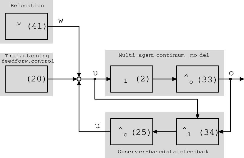
Figure 3: Block diagram of the tracking control scheme with profile relocation. Herein the abbreviations ${\boldsymbol{w}}^{\ast}(t)=[w_{0}^{\ast}(t),w_{\ell}^{\ast}(t)]$, ${\boldsymbol{\kappa}}^{\ast}(t)=[({\boldsymbol{\kappa}}_{0}^{\ast}(t))^{T},({\boldsymbol{\kappa}}_{\ell}^{\ast}(t))^{T}]^{T}$ and $\Delta{\boldsymbol{u}}(t)=[\Delta u_{0}(t),\Delta u_{\ell}]^{T}$ are used.

5.2 Communication topology

The transfer from the continuum description to the discrete formulation is obtained by using a finite difference discretization for the arising PDE models (2), (32) and (39). For the $x$- and $c$-dynamics (and similarly for the $x_{e}$- or $x_{s}$-dynamics) this results in the formulation (1) taking into account Proposition 2 and its proof. This refers to either time-scaling for fixed value of $\ell$ or vice versa. Subsequently, the latter is chosen by keeping $t$ unscaled and setting $\ell=N$ given $N+1$ agents so that $\Delta z=1$. For this choice the reader is also referred to Remark 15.

The observer (32) requires at least the availability of the values $x(z,t)$ at $z\in\{0,\ell\}$ and $\partial_{z}x(z,t)$ at $z=\ell$. Since the observer state is in the considered setting only used to evaluate the feedback controller $\Delta u_{\ell}(t)$ defined in (25b) it is reasonable to evaluate the discretized observer equations at the node $z=\ell$. Alternatively, a distributed evaluation is possible provided that any node has access to the boundary values. The arising integral in (25b) is approximated using the Simpson’s rule.

5.3 Simulation studies

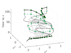
(a) Observer-based 2DOF control with $c(z,t)$ assigned explicitly.

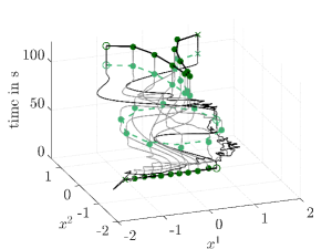
(b) Observer-based 2DOF control with $c(z,t)$ as in (2) but computed in a distributed fashion by PDE (2b).

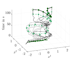
(c) Previous scenario 4(b) but with relocation of final formation center to virtual centre $(1,0)$.

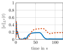
(d) $L^{2}$-norm of tracking error in 4(a).

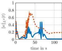
(e) $L^{2}$-norm of tracking error in 4(b).

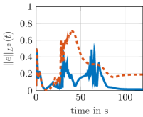
(f) $L^{2}$-norm of tracking error in 4(c).

Figure 4: Consecutive finite time transitions of $N+1=11$ agents from a line formation to an intermediate circle and to a final gull-like formation. The symbols $\circ$ and $\times$ refer to the leader agents at $z=0$ and $z=\ell$ while $\bullet$ denote follower agents. Black lines indicate the initial and the reached final formation, green dashed lines illustrate desired intermediate formation profiles. Top row: spatial-temporal transition paths from the overlay of $x^{1}(z,t)$ and $x^{2}(z,t)$; bottom row: tracking errors with $\|e^{1}\|_{L^{2}}(t)$ in blue and $\|e^{2}\|_{L^{2}}(t)$ in red (dashed).

Two transitions are performed in each of the three simulation scenarios for $N+1=11$ agents ($\ell=10$) illustrated in Fig. 4. In all studies 4(a)-4(c) the agents start with the same line formation at $t=0$ and then move to a circular formation. During the second transition the deployments change from a circle to a gull-like shape. Note that the line formation is stable by design while the circular formation is open-loop unstable for both coordinates. For the gull-like formation the $x^{2}$-coordinate remains open-loop unstable but the coefficient $c^{1}(z,t)$ in the PDE governing $x^{1}(z,t)$ becomes negative, i.e., it changes from an open-loop unstable to a stable formation profile in $x^{1}(z,t)$. In Fig. 4(c) the formation additionally moves to the virtual centre $(1,0)$ using the relocation approach proposed in Section 5.1. Each of the two transitions lasts $50\,$\mathrm{s}$$ and the entire simulation time is set to $120\,$\mathrm{s}$$. The diffusion coefficient in (2) is set to $a^{i}=1$ for all scenarios. These differ in their problem setup:

• Fig. 4(a) shows the transitions obtained with the 2DOF controller with $c^{i}(z,t)=c^{\ast i}(t)$ directly assigned as a Gevrey function, equivalently to (18) with steady state data according to Tab. 2. The position data for the evaluation of (25b) is estimated by the developed state observer.

• The scenario in Fig. 4(b) is identical to the previous study but implements the PDE (2b) for the distributed computation of the reaction coefficient $c(z,t)$ by imposing $d^{i}(z,t)=0$, $b^{i}=(N+1)/2=11/2$ and $v_{0}^{i}(t)=v_{0}^{\ast i}(t)$, $v_{\ell}^{i}(t)=v_{\ell}^{\ast i}(t)$ according to the second elements of the vectors in (20). Note that $b^{i}>a^{i}$ is chosen to obtain a faster convergence of $c^{i}(z,t)$ compared to $x^{i}(z,t)$.

• In Fig. 4(c) additionally the information of the centre point is propagated in a decentralized way through the agent topology by means of the relocation procedure using (39) for $w_{0}(t)$, $w_{\ell}(t)$ designed as feedforward terms following the procedure of Section 3.

The corresponding steady state parameters can be studied from Tab. 2. Controller and observer gains are assigned as $\mu(t)=0.5$ and $\nu(t)=0.6$, respectively, for both coordinates.

Table 2: Desired steady state transition parameters to be taken at time instances $t=\tau_{1}$ and $t=\tau_{2}$.

	$x^{1}(z,t)$			$x^{2}(z,t)$
$t$:	$0$	$\tau_{1}$	$\tau_{2}$	$0$	$\tau_{1}$	$\tau_{2}$
$\bar{x}_{0}^{\ast}$:	$-1$	$1$	$-1$	$0$	$0$	$1$
$\bar{x}_{\ell}^{\ast}$:	$1$	$1$	$1$	$0$	$0$	$1$
$\bar{c}^{\ast}$:	$0$	$(2\pi/\ell)^{2}$	$-(7/\ell)^{2}$	$0$	$(2\pi/\ell)^{2}$	$(2\pi/\ell)^{2}$
$\bar{x}_{\mathrm{e}}^{\ast}$:	$0$	$0$	$1$	$0$	$0$	$0$

To test the robustness of the approach towards the real-time application in Section 6 the following deviations from the nominal case are introduced into any simulation scenario:

• First, the sample time of the boundary control inputs and the observer is set to $t_{s}^{o}=10~{}$\mathrm{ms}$$, while the update interval of the exogenous system (39) and the subsystem for $c(z,t)$ is specified as $t_{s}^{e}=20~{}$\mathrm{ms}$$.

• Second, the propagation of information of the exogenous system (39) and the $c(z,t)$-subsystem require (wireless) communication messages between the agents. For the simulations information drop-outs are induced to model the loss of messages. The consequences of these drop-outs are randomly lagging values of $c(z,t)$ and ${x}_{\mathrm{e}}(z,t)$ for the followers.

• Third, the multi-agent system does not start in its intended line formation but a random initial control and observation error is induced. The error is limited to $\pm 5~{}$\mathrm{\char 37\relax}$$ of the formation amplitude, e.g., here $\left|\tilde{x}(z,t)\right|\leq 0.05$ given the circle radius is $1$.

Under these circumstances the performance of the control concept can be evaluated by studying Figs. 4(d)-4(f) which show the $L^{2}$-norm of the tracking errors $e^{1}(z,t)$ and $e^{2}(z,t)$ for the three simulation scenarios. Despite the imposed errors the 2DOF control concept is in any studied case capable of realizing stable transitions between the different formations profiles. The introduction of the $c$-subsystem (2b), (2d) to distribute parameter information involving simulated information drop-outs and the relocation of the centre point from $(0,0)$ to $(1,0)$ as expected yield slightly larger tracking errors during transient behavior.

6 Experimental results

Experimental results are presented from a laboratory test rig at the Chair of Control, Kiel University. To the best knowledge of the authors this represents the first real-time implementation of the backstepping methodology based on parabolic PDEs for the formation control of multi-agent systems using continuum models.

6.1 Multi robot test rig

Basically the multi-agent system is built upon small caterpillar robots which are shown Fig. 5, where in addition the basic features of the used robot are listed to give an impression of the available computational power and memory capacity.

Type	Features
Processor	ARM Cortex-M4F $120$MHz
RAM	$2\times 64$kB
Flash	$512$kB
Communication	USB, nRF$24$, Bluetooth
Motors	$2$ DC motors with $75:1$ gearbox
Periphery	$6$ axis IMU, $2$ LEDs, Buzzer,
	Magentic quadrature encoders,
	IR sensors, Arduino header, etc.
Dimensions	approx. $10$cm $\times$ $10$cm $\times$ $4$cm

Figure 5: The agent: a wheeled caterpillar robot (Styger, 2016).

The real-time implementation of the 2DOF control concept introduced in Sections 3 and 4 demands to access the position of each robot agent in the two dimensional plane either by measurement or by using the state observer. To address this a suitable hard- and software environment has been set up to perform controlled transitions between different formations including their relocation. The used environment is schematically illustrated in Fig. 6 and basically consists of the four main subsystems:

1. Ceiling-mounted camera or a camera system for optical position detection.

2. Computer for OpenCV application (Bradski, 2000).

3. Development board with a radio module.

4. Caterpillar robots equipped with AruCo codes (Garrido-Jurado et al., 2014).

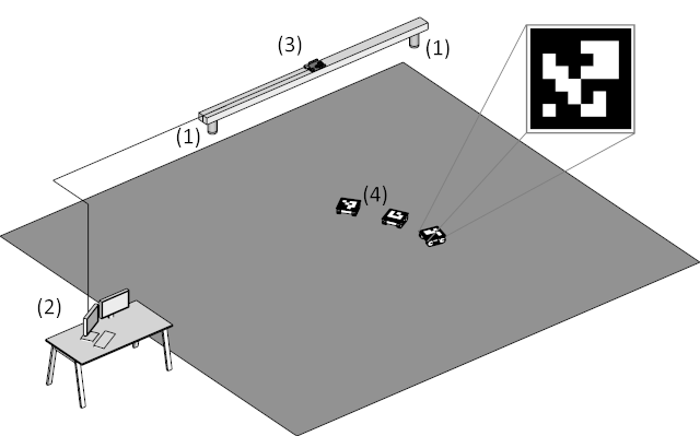
Figure 6: Basic scheme of the mobile robot test rig.

In the test environment a ceiling-mounted camera is used for global position measurement and subsequently emulates the induced communication topology of the multi-agent system. For this, a work station runs an image processing application which uses OpenCV and includes the so-called AruCo library. The latter is used to detect the individual AruCo codes, which are fixed on top of each agent (Garrido-Jurado et al., 2014). The image data is processed and is sent via a serial interface to an electronic development board, which is equipped with a radio module. The electronic board runs a software which broadcasts messages with the position information of all agents via radio to the caterpillar robots. The caterpillar robots, serving as agents, are equipped with two DC motors and a radio module. From the broadcast each robot only extracts its specific position information according to the underlying communication topology, which is induced by the input protocol (1a).

Remark 14.

It should be emphasised that the used caterpillar robot represents a non-holonomic system. Its kinematic model has the form $\dot{x}^{1}_{r}(t)=v_{r}(t)\cos(\phi_{r}(t))$, $\dot{x}^{2}_{r}(t)=v_{r}(t)\sin(\phi_{r}(t))$, $\dot{\phi}_{r}(t)=\omega_{r}(t)$ with $v_{r}(t)$ the translational velocity and $\omega_{r}(t)$ the angular velocity defining the robot orientation $\phi_{r}(t)$ in the 2D plane. Obviously the model has to satisfy the non-holonomic constraint $\dot{x}^{2}_{r}(t)\cos(\phi_{r}(t))=\dot{x}^{1}_{r}(t)\sin(\phi_{r}(t))$. This behaviour, induced by the robot kinematics, somewhat counteracts the modeling assumptions, where the agents are in principle represented as ideal mass points. Moreover, it provides a significant challenge for the developed 2DOF controllers to compensate this difference hence imposing a benchmark for robustness analysis.

6.2 Test scenario

The experimental results for $N+1=11$ robots are based on the follower protocol (1a) and the leader protocol (1c) imposed by the discretization described in Section 5.2. The time-variant reaction term $c_{j}^{i}(t)$, $i=1,2$, $j=0,1,\ldots,10$ is for ease of implementation configured off-line for each agent. The synchronisation of the temporal evolution of the parameter for all agents is reached through a trigger signal, which is broadcasted via radio. The implementation of the leader protocol involves the 2DOF controller consisting of the flatness-based feedforward term (20) and a measurement-based backstepping controller according to (25a), (25b), respectively.

Remark 15.

In the numerical simulations it is possible to fix $\ell$ and to adjust $N$ so that the discretization stepsize $\Delta z=\ell/N$ in principle becomes arbitrarily small for $N\gg 1$. For a numerically stable integration of the resulting ODEs this necessitates to choose a sufficiently small time step $\Delta t$ for numerical stability. This is no longer possible at the experimental setup since the time step is imposed by the minimal sampling time, which depends on the used sensor, actuation, communication, and processing devices involved in the control loop. To address this, $\ell=N$ is chosen both in the simulation and the experimental results. Note that this choice is in line with exposition in Proposition 2.

The obtained experimental results are shown in Fig. 8(a) for the twofold transition: first from the initial line configuration passing through the point $(-150,0)\,$\mathrm{c}\mathrm{m}$$ to an intermediate half circle formation of radius $R=150\,$\mathrm{c}\mathrm{m}$$ within the time interval $t\in[0,\tau]$ and secondly to a desired circle formation of radius $R$ within the time interval $t\in(\tau,2\tau]$ (see also Fig. 7). Herein, the feedforward term and the integral kernel (24) are computed off-line and are implemented using linear interpolation. The parameter setting for the experiment is listed in Tab. 3. In view of the parameter values and the ansatz (10) the desired steady state solutions for $t=2\tau$ can be written as

$$\bar{x}^{1,\ast}(z)=-R\cos(\omega z),~{}\bar{x}^{2,\ast}(z)=-R\sin(\omega z)$$

with $\omega={2\pi}/{(\ell+1)}$. Differing from the simulation studies before the spatial period $\omega$ of the $\sin$- and $\cos$-functions is reduced from $2\pi/\ell$ to $2\pi/(\ell+1)$ and the values for $\bar{x}_{0}^{i,\ast}$, $\bar{x}_{\ell}^{i,\ast}$, $i=1,2$ are shifted appropriately. Since no explicit collision avoidance algorithm is used during the transitions this choice of $\omega$ implies that the leader nodes $z=\{0,\ell\}$ are separated (for $\omega=2\pi/\ell$ in both leaders will be located at the same point in the circular formation). For comparison reasons and to illustrate the performance of the 2DOF control concept in Fig. 8(b) experimental results are provided for the combination of the flatness-based feedforward control with proportional error control at the leader agents in the form (25a), i.e., $\Delta u_{0}(t)=-\mu(t)e(0,t)$ and $\Delta u_{\ell}(t)=-\mu(t)e(\ell_{\mathrm{}},t)$ with $\mu(t)=0.15$. The mean distance error

$$\tilde{r}_{\mathrm{m}}(t) =\frac{1}{N+1}\sum_{j=0}^{N}\tilde{r}_{i}(t)$$ (40)

with $(\tilde{r}_{i}(t))^{2}={(x^{1}_{j}(t)-x^{\ast,1}_{j}(t))^{2}+(x^{2}_{j}(t)-x^{\ast,2}_{j}(t))^{2}}.$ between desired and measured position values is shown in Fig. 8(c) and Fig. 8(d). Analysing the results of Fig. 8 clearly reveals that the 2DOF controller including the backstepping-based error feedback is able to stabilise the transitions while the simple proportional error feedback fails and the desired formation falls apart.

Figure 7: Snapshots of the transition using the ceiling-mounted camera system.

Table 3: Parameters for the test scenario with $a=0.5$, $\ell=10$ and $\tau=80$ s. Geometric values are given in cm.

	$t$	$0$	$\tau$	$2\tau$
Coord. $1$:	$\bar{x}_{0}^{\ast}$	$150$	$0$	$-150$
	$\bar{x}_{\ell}^{\ast}$	$150$	$0$	$-150\cos(2\pi\ell/(\ell+1))$
	$\bar{c}^{\ast}$	$0$	$a(\pi/\ell)^{2}$	$a(2\pi/(\ell+1))^{2}$
Coord. $2$:	$\bar{x}_{0}^{\ast}$	$-150$	$-150$	$0$
	$\bar{x}_{\ell}^{\ast}$	$\phantom{-}150$	$\phantom{-}150$	$-150\sin(2\pi\ell/(\ell+1))$
	$\bar{c}^{\ast}$	$0$	$a(\pi/\ell)^{2}$	$a(2\pi/(\ell+1))^{2}$

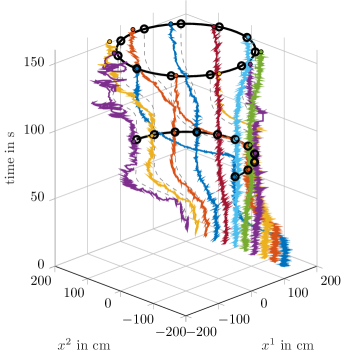
(a) Flatness-based feedforward control with backstepping-
based error feedback.

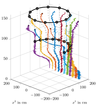
(b) Flatness-based feedforward control with proportional error feedback.

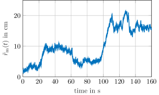
(c) Mean distance error for 8(a).

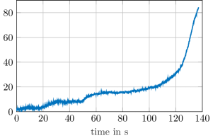
(d) Mean distance error for 8(b).

Figure 8: Experimental results for the test scenario. 8(a) shows the spatial-temporal evolution of the transition with 2DOF controller including a backstepping-based feedback term; for 8(b) the 2DOF controller is evaluated with a proportional error feedback; 8(c) and 8(d) show the mean distance error computed according to (40).

7 Conclusion

Based on a continuum model in terms of coupled PDEs a 2DOF control concept is developed for the deployment of multi-agent systems into desired formation profiles. Diffusion-reaction equations are set up to govern the spatial-temporal agent dynamics in the plane and simultaneously enabling us to also distribute (decentralized) parameter information. Based on the PDE model flatness-based trajectory planning is addressed and combined with backstepping-based state feedback control to achieve the stable tracking of desired spatial-temporal profiles. For the required state estimation a backstepping-based Luenberger observer is designed and integrated into the closed-loop control. With this, finite time transitions between desired formation profiles, which are determined as possibly unstable steady state solutions of the governing PDEs, can be realized. Due to inclusion of time variant parameters this includes the connection between different families of steady states. The distribution and propagation of parameter values between the agents is directly incorporated into the setting in terms of a feedforward control approach. Furthermore the incorporation of an exogenous system enables us to achieve the spatial relocation of the formation. The transfer of the determined controller and estimation algorithms to the finite-dimensional discrete multi-agent network is achieved using finite difference discretization. Depending on the PDE model this may even result in a decentralised implementation and directly imposes the necessary chain-like communication topology. Simulations studies show the tracking performance and the robustness of the concept even in view of rather challenging deviations from the expected behaviour. These findings are confirmed also in first experimental results conducted with a small swarm of caterpillar robots. By means of the developed 2DOF control concept transitions between different and also unstable (with respect to the considered PDEs) formation profiles are achieved. To the best knowledge of the authors the presented results are the first real-time implementation of the backstepping methodology for parabolic PDEs and the use of controllers based on continuum models for multi-agent systems.

The financial support by the Deutsche Forschungsgesellschaft (DFG) in the individual grant ref. 266006167 is gratefully acknowledged. The authors would like to thank Prof. Erich Styger from Lucerne University of Applied Sciences and Arts for his support concerning the embedded computing facilities of the used caterpillar robots, Simon Helling for his help during the implementation of the algorithms at the experimental set-up, and Dr. Petro Feketa for thoughtful discussions concerning the well-posedness analysis.

References

- Baccoli et al. (2015) A. Baccoli, A. Pisano, and Y. Orlov. Boundary control of coupled reaction–diffusion processes with constant parameters. Automatica, 54(Supplement C):80–90, April 2015.
- Balch and Arkin (1998) T. Balch and R. C. Arkin. Behavior-based formation control for multirobot teams. IEEE Transactions on Robotics and Automation, 14(6):926–939, December 1998.
- Bradski (2000) G. Bradski. The OpenCV Library. Dr. Dobb’s Journal of Software Tools, 2000. Accessed: 2018-11-08.
- Bullo (2018) F. Bullo. Lectures on Network Systems. CreateSpace, 1 edition, 2018. With contributions by J. Cortes, F. Dorfler, and S. Martinez.
- Coron and Trélat (2004) J.-M. Coron and E. Trélat. Global steady–state controllability of 1–d semilinear heat equations. SIAM J. Control Optim., 43(2):549–569, 2004.
- Dörfler and Bullo (2014) F. Dörfler and F. Bullo. Synchronization in complex networks of phase oscillators: A survey. Automatica, 50(6):1539–1564, June 2014.
- Easley and Kleinberg (2010) D. Easley and J. Kleinberg. Networks, Crowds, and Markets: Reasoning about a Highly Connected World. Cambridge University Press, 2010.
- Freudenthaler and Meurer (2016) G. Freudenthaler and T. Meurer. PDE-based tracking control for multi-agent deployment. IFAC-PapersOnLine, 49(18):582–587, 2016.
- Freudenthaler et al. (2017) G. Freudenthaler, F. Göttsch, and T. Meurer. Backstepping-based extended Luenberger observer design for a Burgers-type PDE for multi-agent deployment. IFAC-PapersOnLine, 50(1):6780–6785, 2017. 20th IFAC World Congress.
- Frihauf and Krstic (2011) P. Frihauf and M. Krstic. Leader-Enabled Deployment Onto Planar Curves: A PDE-Based Approach. IEEE Transactions on Automatic Control, 56(8):1791–1806, 2011.
- Garrido-Jurado et al. (2014) S. Garrido-Jurado, R. Muñoz-Salinas, F. J. Madrid-Cuevas, and M. J. Marín-Jiménez. Automatic generation and detection of highly reliable fiducial markers under occlusion. Pattern Recognition, 47(6):2280–2292, June 2014.
- Jadachowski et al. (2012) L. Jadachowski, T. Meurer, and A. Kugi. An Efficient Implementation of Backstepping Observers for Time-Varying Parabolic PDEs. IFAC Proceedings Volumes, 45(2):798–803, January 2012.
- Krstic and Smyshlyaev (2008) M. Krstic and A. Smyshlyaev. Boundary Control of PDEs: A Course on Backstepping Designs. SIAM, Philadelphia, 2008.
- Kubrusly (2011) C.S. Kubrusly. The Elements of Operator Theory. Birkhäuser Boston, 2011. ISBN 9780817649982.
- Laroche et al. (2000) B. Laroche, P. Martin, and P. Rouchon. Motion planning for the heat equation. Int. J. Robust Nonlinear Control, 10:629–643, 2000.
- Leonard and Fiorelli (2001) N. E. Leonard and E. Fiorelli. Virtual leaders, artificial potentials and coordinated control of groups. In Proceedings of the 40th IEEE Conference on Decision and Control (Cat. No.01CH37228), volume 3, pages 2968–2973 vol.3, 2001.
- Liang et al. (2003) J. Liang, R. Nagel, and T.J. Xiao. Nonautonomous heat equations with generalized Wentzell boundary conditions. J. Evol. Equ., pages 321–331, 2003.
- Mesbahi and Egerstedt (2010) M. Mesbahi and M. Egerstedt. Graph Theoretic Methods in Multiagent Networks. Princeton University Press, 2010.
- Meurer (2013) T. Meurer. Control of Higher–Dimensional PDEs. Communications and Control Engineering. Springer, 2013.
- Meurer and Krstic (2011) T. Meurer and M. Krstic. Finite-time multi-agent deployment: A nonlinear PDE motion planning approach. Automatica, 47(11):2534–2542, 2011.
- Meurer and Kugi (2009a) T. Meurer and A. Kugi. Tracking control for boundary controlled parabolic PDEs with varying parameters: Combining backstepping and differential flatness. Automatica, 45(5):1182–1194, 2009a.
- Meurer and Kugi (2009b) T. Meurer and A. Kugi. Trajectory Planning for Boundary Controlled Parabolic PDEs With Varying Parameters on Higher-Dimensional Spatial Domains. IEEE Transactions on Automatic Control, 54(8):1854–1868, August 2009b.
- Motsch and Tadmor (2014) S. Motsch and E. Tadmor. Heterophilious Dynamics Enhances Consensus. SIAM Review, 56(4):577–621, 2014.
- Murray (2007) R.M. Murray. Recent Research in Cooperative Control of Multivehicle Systems. Journal of Dynamic Systems, Measurement, and Control, 129(5):571–583, September 2007.
- Olfati-Saber (2006) R. Olfati-Saber. Flocking for multi-agent dynamic systems: algorithms and theory. IEEE Transactions on Automatic Control, 51(3):401–420, March 2006.
- Olfati-Saber et al. (2007) R. Olfati-Saber, J. A. Fax, and R. M. Murray. Consensus and Cooperation in Networked Multi-Agent Systems. Proceedings of the IEEE, 95(1):215–233, January 2007.
- Pilloni et al. (2016) A. Pilloni, A. Pisano, Y. Orlov, and E. Usai. Consensus-Based Control for a Network of Diffusion PDEs With Boundary Local Interaction. IEEE Transactions on Automatic Control, 61(9):2708–2713, 2016.
- Qi et al. (2015) J. Qi, R. Vazquez, and M. Krstic. Multi-Agent Deployment in 3-D via PDE Control. IEEE Transactions on Automatic Control, 60(4):891–906, 2015.
- Reynolds (1987) C.W. Reynolds. Flocks, Herds and Schools: A Distributed Behavioral Model. In Proceedings of the 14th Annual Conference on Computer Graphics and Interactive Techniques, SIGGRAPH ’87, pages 25–34, New York, NY, USA, 1987. ACM.
- Rodino (1993) L. Rodino. Gevrey functions and ultradistributions. In Linear Partial Differential Operators in Gevrey Spaces, pages 5–59. WORLD SCIENTIFIC, March 1993.
- Rudolph et al. (2005) J. Rudolph, J. Winkler, and F. Woittennek. Flatness based approach to a heat conduction problem in a crystal growth process. In T. Meurer, K. Graichen, and E.D. Gilles, editors, Control and Observer Design for Nonlinear Finite- and Infinite-Dimensional Systems, Lecture Notes in Control and Information Sciences, pages 387–401. Springer-Verlag, Berlin, 2005.
- Smyshlyaev and Krstic (2004) A. Smyshlyaev and M. Krstic. Closed-form boundary state feedbacks for a class of 1-D partial integro-differential equations. IEEE Transactions on Automatic Control, 49(12):2185–2202, 2004.
- Smyshlyaev and Krstic (2005) A. Smyshlyaev and M. Krstic. Backstepping observers for a class of parabolic PDEs. Systems & Control Letters, 54(7):613–625, 2005.
- Styger (2016) E. Styger. Personal communication, October 2016.
- Vazquez et al. (2008) R. Vazquez, E. Trélat, and J.-M. Coron. Control for fast and stable Laminar-to-High-Reynolds-Numbers transfer in a 2D Navier-Stokes channel flow. Discrete & Continuous Dynamical Systems - B, 10(4):925–956, 2008.
- Zuazua (2018) E. Zuazua. Personal communication, October 2018.