Mixed Spatial and Temporal Decompositions for Large Scale Multistage Stochastic Optimization Problems

Abstract

We consider multistage stochastic optimization problems involving multiple units. Each unit is a (small) control system. Static constraints couple units at each stage. We present a mix of spatial and temporal decompositions to tackle such large scale problems. More precisely, we obtain theoretical bounds and policies by means of two methods, depending whether the coupling constraints are handled by prices or by resources. We study both centralized and decentralized information structures. We report the results of numerical experiments on the management of urban microgrids. It appears that decomposition methods are much faster and give better results than the standard Stochastic Dual Dynamic Programming method, both in terms of bounds and of policy performance.

1 Introduction

Multistage stochastic optimization problems are, by essence, complex because their solutions are indexed both by stages (time) and by uncertainties (scenarios). Another layer of complexity can come from spatial structure. The large scale nature of such problems makes decomposition methods appealing (we refer to [17, 8] for a broad description of decomposition methods in stochastic optimization problems).

We sketch decomposition methods along three dimensions: temporal decomposition methods like Dynamic Programming break the multistage problem into a sequence of interconnected static subproblems [3, 5]; scenario decomposition methods split large scale stochastic optimization problems scenario by scenario, yielding deterministic subproblems [15, 20, 11]; spatial decomposition methods break possible spatial couplings in a global problem to obtain local decoupled subproblems [9]. These decomposition schemes have been applied in many fields, and especially in energy management: Dynamic Programming methods have been used for example in dam management [18], and scenario decomposition has been successfully applied to the resolution of unit-commitment problems [1], among others.

Recent developments have mixed spatial decomposition methods with Dynamic Programming to solve large scale multistage stochastic optimization problems. This work led to the introduction of the Dual Approximate Dynamic Programming (DADP) algorithm, which was first applied to unit-commitment problems with a single central coupling constraint linking different stocks [2], and later applied to dams management problems [6]. This article moves one step further by considering altogether two types of decompositions (by prices and by resources) when dealing with general coupling constraints among units. General coupling constraints often arise from flows conservation on a graph, and our motivation indeed comes from district microgrid management, where buildings (units) consume, produce and store energy and are interconnected through a network.

The paper is organized as follows. In Sect. 2, we introduce a generic stochastic multistage problem with different subsystems linked together via a set of static coupling constraints. We present price and resource decomposition schemes, that make use of so-called admissible coordination processes. We show how to bound the global Bellman functions above by a sum of local resource-decomposed value functions, and below by a sum of local price-decomposed value functions. In Sect. 3, we study the special case of deterministic coordination processes. First, we show that the local price and resource decomposed value functions satisfy recursive Dynamic Programming equations. Second, we outline how to improve the bounds. Third, we show how to use the decomposed Bellman functions to devise admissible policies for the global problem. Finally, we provide an analysis of the decentralized information structure, that is, when the controls of a given subsystem only depend on the past observations of the noise in that same subsystem. In Sect. 4, we present numerical results for the optimal management of different microgrids of increasing size and complexity. We compare the two decomposition algorithms with (state of the art) Stochastic Dual Dynamic Programming (SDDP) algorithm. The analysis of case studies consisting of district microgrids coupling up to 48 buildings together enlightens that decomposition methods give better results in terms of cost performance, and achieve up to a four times speedup in terms of computational time.

2 Upper and Lower Bounds by Spatial Decomposition

We focus in §2.1 on a generic decomposable optimization problem and present price and resource decomposition schemes. In §2.2, we apply these two methods to a multistage stochastic optimization problem, by decomposing a global static coupling constraint by means of so-called price and resource coordination processes. For such problems, we define the notions of centralized and decentralized information structures.

2.1 Bounds for an Optimization Problem under Coupling Constraints via Decomposition

In §2.1.1, we introduce a generic optimization problem with coupled local units. In §2.1.2, we show how to bound its optimal value by decomposition.

2.1.1 Global Optimization Problem Formulation

Let $\mathfrak{N}$ be a finite set, representing local units $n\in\mathfrak{N}$ (we use the letter $\mathfrak{N}$ as units can be seen as nodes on a graph). Let $\left\{\mathcal{Z}^{n}\right\}_{n\in\mathfrak{N}}$ be a family of sets and $J^{n}:\mathcal{Z}^{n}\rightarrow]-\infty,+\infty]$, $n\in\mathfrak{N}$, be local criteria, one for each unit, taking values in the extended reals $]-\infty,+\infty]$ ($+\infty$ included to allow for possible constraints). Let $\left\{\mathcal{R}^{n}\right\}_{n\in\mathfrak{N}}$, be a family of vector spaces and $\vartheta^{n}:\mathcal{Z}^{n}\rightarrow\mathcal{R}^{n}$, $n\in\mathfrak{N}$, be mappings that model local constraints.

From these local data, we formulate a global minimization problem under constraints. We define the product set $\mathcal{Z}=\prod_{n\in\mathfrak{N}}\mathcal{Z}^{n}$ and the product space $\mathcal{R}=\prod_{n\in\mathfrak{N}}\mathcal{R}^{n}$. Finally, we introduce a subset $S\subset\mathcal{R}$ that captures the coupling constraints between the $N$ units. Using the notation $z=\left\{z^{n}\right\}_{n\in\mathfrak{N}}$, we define the global optimization problem as

$$V{\sharp}=\inf_{z\in\mathcal{Z}}\;\sum_{n\in\mathfrak{N}}J^{n}(z^{n})\;,$$ (1a)

under the global coupling constraint

$$\big{\{}{\vartheta^{n}(z^{n})}\big{\}}_{n\in\mathfrak{N}}\in-S\;.$$ (1b)

The set $S$ is called the primal admissible set, and an element $\left\{r^{n}\right\}_{n\in\mathfrak{N}}\in-S$ is called an admissible resource vector. We note that, without Constraint (1b), Problem (1) would decompose into $|\mathfrak{N}|$ independent subproblems in a straightforward manner.

We moreover assume that, for $n\in\mathfrak{N}$, the space $\mathcal{R}^{n}$ (resources) is paired with a space $\mathcal{P}^{n}$ (prices) by bilinear forms $\big{\langle}{\cdot,\,\cdot}\big{\rangle}\;:\;\mathcal{P}^{n}\times\mathcal{R}^{n}\to{\mathbb{R}}$ (duality pairings). We define the product space $\mathcal{P}=\prod_{n\in\mathfrak{N}}\mathcal{P}^{n}$, so that $\mathcal{R}$ and $\mathcal{P}$ are paired by the duality pairing $\big{\langle}{p,\,r}\big{\rangle}=\sum_{n\in\mathfrak{N}}\big{\langle}{p^{n},\,r^{n}}\big{\rangle}$ (see [14] for further details; a typical example of paired spaces is a Hilbert space and itself).

2.1.2 Upper and Lower Bounds from Price and Resource Value Functions

Consider the global optimization problem (1). For each $n\in\mathfrak{N}$, we introduce local price value functions $\underline{V}^{n}:\mathcal{P}^{n}\to[-\infty,+\infty[$ defined by

$$\underline{V}^{n}[{p^{n}}]=\inf_{z^{n}\in\mathcal{Z}^{n}}\;J^{n}(z^{n})+\big{\langle}{p^{n},\,\vartheta^{n}(z^{n})}\big{\rangle}\;,$$ (2)

where we have supposed that $V^{n}[{p^{n}}]<+\infty$, and local resource value functions $\overline{V}^{n}:\mathcal{R}^{n}\to]-\infty,+\infty]$ defined by

$$\overline{V}^{n}[{r^{n}}]=\inf_{z^{n}\in\mathcal{Z}^{n}}\;J^{n}(z^{n})\quad\text{s.t.}\ \quad\vartheta^{n}(z^{n})=r^{n}\;,$$ (3)

where we have supposed that $\overline{V}^{n}[{r^{n}}]>-\infty$,

We denote by $S^{\star}\subset\mathcal{P}$ the dual cone associated with the constraint set $S$:

$$S^{\star}=\big{\{}{p\in\mathcal{P}\;|\;\big{\langle}{p,\,r}\big{\rangle}\geq 0\;,\enspace\forall r\in S}\big{\}}\;.$$ (4)

The cone $S^{\star}$ is called the dual admissible set, and an element $\left\{p^{n}\right\}_{n\in\mathfrak{N}}\in S^{\star}$ is called an admissible price vector. We now establish lower and upper bounds for Problem (1), and show how they can be computed in a decomposed way, that is, unit by unit.

Proposition 1

For any admissible price vector $p=\left\{p^{n}\right\}_{n\in\mathfrak{N}}\in S^{\star}$ and for any admissible resource vector $r=\left\{r^{n}\right\}_{n\in\mathfrak{N}}\in-S$, we have the following lower and upper decomposed estimates of the global minimum $V{\sharp}$ of Problem (1):

$$\sum_{n\in\mathfrak{N}}\underline{V}^{n}[{p^{n}}]\;\leq\;V{\sharp}\;\leq\;\sum_{n\in\mathfrak{N}}\overline{V}^{n}[{r^{n}}]\;.$$ (5)

Proof. Because we have supposed that $V^{n}[{p^{n}}]<+\infty$, the left hand side of Equation (5) belongs to $[-\infty,+\infty[$. In the same way, the right hand side belongs to $]-\infty,+\infty]$. For a given $p=\left\{p^{n}\right\}_{n\in\mathfrak{N}}\in S^{\star}$, we have

$$\sum_{n\in\mathfrak{N}}\underline{V}^{n}[{p^{n}}] =\sum_{n\in\mathfrak{N}}\inf_{z^{n}\in\mathcal{Z}^{n}}\;J^{n}(z^{n})+\big{\langle}{p^{n},\,\vartheta^{n}(z^{n})}\big{\rangle}\;,$$

$$=\inf_{z\in\mathcal{Z}}\;{\sum_{n\in\mathfrak{N}}J^{n}(z^{n})}+\big{\langle}{p,\,\left\{\vartheta^{n}(z^{n})\right\}_{n\in\mathfrak{N}}}\big{\rangle}\;, z=\left\{z^{n}\right\}_{n\in\mathfrak{N}}$$ (since )

$$\leq\inf_{z\in\mathcal{Z}}\;{\sum_{n\in\mathfrak{N}}J^{n}(z^{n})}+\big{\langle}{p,\,\left\{\vartheta^{n}(z^{n})\right\}_{n\in\mathfrak{N}}}\big{\rangle}\;,$$

$$\hphantom{\leq\inf_{z\in\mathcal{Z}}}\text{s.t.}\ {\left\{\vartheta^{n}(z^{n})\right\}_{n\in\mathfrak{N}}}\in-S$$ (minimizing on a smaller set)

$$\leq\inf_{z\in\mathcal{Z}}\;{\sum_{n\in\mathfrak{N}}J^{n}(z^{n})+0} p\in S^{\star} S^{\star}$$ (as and by definition (4) of )

$$\hphantom{\leq\inf_{z\in\mathcal{Z}}}\text{s.t.}\ {\left\{\vartheta^{n}(z^{n})\right\}_{n\in\mathfrak{N}}}\in-S\;,$$

which gives the lower bound inequality.

The upper bound is easily obtained, as the optimal value $V{\sharp}$ of Problem (1) is given by $\inf_{\tilde{r}\in-S}\sum_{n\in\mathfrak{N}}\overline{V}^{n}[{\tilde{r}^{n}}]\leq\sum_{n\in\mathfrak{N}}\overline{V}^{n}[{r^{n}}]$ for any $r\in-S$. $\Box$

2.2 The Special Case of Multistage Stochastic Optimization Problems

Now, we turn to the case where Problem (1) corresponds to a multistage stochastic optimization problem elaborated from local data (local states, local controls, and local noises), with global coupling constraints at each time step. We use the notation $\llbracket r,s\rrbracket=\{{r,r+1,\ldots,s-1,s}\}$ for two integers $r\leq s$, and we consider a time span $\llbracket 0,T\rrbracket$ where $T\in{\mathbb{N}}^{\star}$ is a finite horizon.

2.2.1 Local Data for Local Stochastic Control Problems

We detail the local data describing each unit. Let $\big{\{}{{\mathbb{X}}_{t}^{n}}\big{\}}_{t\in\llbracket 0,T\rrbracket}$, $\big{\{}{{\mathbb{U}}_{t}^{n}}\big{\}}_{t\in\llbracket 0,T-1\rrbracket}$ and $\big{\{}{{\mathbb{W}}_{t}^{n}}\big{\}}_{t\in\llbracket 1,T\rrbracket}$ be sequences of measurable spaces for each unit $n\in\mathfrak{N}$. We consider two other sequences of measurable vector spaces $\big{\{}{\mathcal{R}_{t}^{n}}\big{\}}_{t\in\llbracket 0,T-1\rrbracket}$ and $\big{\{}{\mathcal{P}_{t}^{n}}\big{\}}_{t\in\llbracket 0,T-1\rrbracket}$ such that for all $t$, $\mathcal{R}_{t}^{n}$ and $\mathcal{P}_{t}^{n}$ are paired spaces, equipped with a bilinear form $\big{\langle}\cdot\>,\cdot\big{\rangle}$. We also introduce, for all $n\in\mathfrak{N}$ and for all $t\in\llbracket 0,T-1\rrbracket$,

• measurable local dynamics $g_{t}^{n}:{\mathbb{X}}_{t}^{n}\times{\mathbb{U}}_{t}^{n}\times{\mathbb{W}}_{t+1}^{n}\to{\mathbb{X}}_{t+1}^{n}$,

• measurable local coupling functions $\Theta_{t}^{n}:{\mathbb{X}}_{t}^{n}\times{\mathbb{U}}_{t}^{n}\to\mathcal{R}_{t}^{n}$,

• measurable local instantaneous costs $L_{t}^{n}:{\mathbb{X}}_{t}^{n}\times{\mathbb{U}}_{t}^{n}\times{\mathbb{W}}_{t+1}^{n}\rightarrow]-\infty,+\infty]$,

and a measurable local final cost $K^{n}:{\mathbb{X}}^{n}_{T}\rightarrow]-\infty,+\infty]$. We incorporate possible local constraints (for instance constraints coupling the control with the state) directly in the instantaneous costs $L_{t}^{n}$ and the final cost $K^{n}$, since they are extended real valued functions which can possibly take the value $+\infty$.

From local data given above, we define the global state, control, noise, resource and price spaces at time $t$ as

$${\mathbb{X}}_{t}=\prod_{n\in\mathfrak{N}}{\mathbb{X}}_{t}^{n},\;\>{\mathbb{U}}_{t}=\prod_{n\in\mathfrak{N}}{\mathbb{U}}_{t}^{n},\;\>{\mathbb{W}}_{t}=\prod_{n\in\mathfrak{N}}{\mathbb{W}}_{t}^{n},\;\>\mathcal{R}_{t}=\prod_{n\in\mathfrak{N}}\mathcal{R}_{t}^{n},\;\>\mathcal{P}_{t}=\prod_{n\in\mathfrak{N}}\mathcal{P}_{t}^{n}\;.$$

We suppose given a global constraint set $S_{t}\subset\mathcal{R}_{t}$ at time $t$. We define the global resource and price spaces $\mathcal{R}$ and $\mathcal{P}$, and the global constraint set $S\subset\mathcal{R}$, as

$$\mathcal{R}=\prod_{t=0}^{T-1}\mathcal{R}_{t}\;,\enspace\mathcal{P}=\prod_{t=0}^{T-1}\mathcal{P}_{t}\;,\enspace S=\prod_{t=0}^{T-1}S_{t}\subset\mathcal{R}\;,$$ (6)

and we denote by $S^{\star}\subset\mathcal{P}$ the dual cone of $S$ (see Equation (4)).

2.2.2 Centralized and Decentralized Information Structures

We introduce a probability space $(\Omega,\mathcal{F},{\mathbb{P}})$. For every unit $n\in\mathfrak{N}$, we introduce local exogenous noise processes $\boldsymbol{W}^{n}=\{{\boldsymbol{W}_{t}^{n}}\}_{t\in\llbracket 1,T\rrbracket}$, where each $\boldsymbol{W}_{t}^{n}:\Omega\to{\mathbb{W}}_{t}^{n}$ is a random variable. We denote by

$$\boldsymbol{W}=(\boldsymbol{W}_{1},\cdots,\boldsymbol{W}_{T})\quad\text{ where }\quad\boldsymbol{W}_{t}=\left\{\boldsymbol{W}_{t}^{n}\right\}_{n\in\mathfrak{N}}$$ (7)

the global noise process.

We consider two information structures [7, Chap. 3]:

• the centralized information structure, represented by the filtration $\mathcal{F}=({\mathcal{F}_{t}})_{t\in\llbracket 0,T\rrbracket}$, associated with the global noise process $\boldsymbol{W}$ in (7), where

  $$\mathcal{F}_{t}=\sigma(\boldsymbol{W}_{1},\cdots,\boldsymbol{W}_{t})=\sigma\big{(}{\left\{\boldsymbol{W}_{1}^{n}\right\}_{n\in\mathfrak{N}},\cdots,\left\{\boldsymbol{W}_{t}^{n}\right\}_{n\in\mathfrak{N}}}\big{)}$$ (8a)

  is the $\sigma$-field generated by all noises up to time $t\in\llbracket 0,T\rrbracket$, with the convention $\mathcal{F}_{0}=\{\emptyset,\Omega\}$,

• the decentralized information structure, represented by the family $\left\{\mathcal{F}^{n}\right\}_{n\in\mathfrak{N}}$ of filtrations $\mathcal{F}^{n}=({\mathcal{F}_{t}^{n}})_{t\in\llbracket 0,T\rrbracket}$, where, for any unit $n\in\mathfrak{N}$ and any time $t\in\llbracket 0,T\rrbracket$,

  $$\mathcal{F}_{t}^{n}=\sigma(\boldsymbol{W}_{1}^{n},\cdots,\boldsymbol{W}_{t}^{n})\subset\mathcal{F}_{t}=\bigvee_{n^{\prime}\in\mathfrak{N}}\mathcal{F}_{t}^{n^{\prime}}\;,$$ (8b)

  with $\mathcal{F}_{0}^{n}=\{\emptyset,\Omega\}$. The local $\sigma$-field $\mathcal{F}_{t}^{n}$ captures the information provided by the uncertainties up to time $t$, but only in unit $n$.

In the sequel, for a given filtration $\mathcal{G}$ and a given measurable space ${\mathbb{Y}}$, we denote by ${\mathbb{L}}^{0}(\Omega,\mathcal{G},{\mathbb{P}};{\mathbb{Y}})$ the space of $\mathcal{G}$-adapted processes taking values in the space ${\mathbb{Y}}$.

2.2.3 Global Stochastic Control Problem

We denote by $\boldsymbol{X}_{t}=\left\{\boldsymbol{X}_{t}^{n}\right\}_{n\in\mathfrak{N}}$ and $\boldsymbol{U}_{t}=\left\{\boldsymbol{U}_{t}^{n}\right\}_{n\in\mathfrak{N}}$ families of random variables (each of them with values in ${\mathbb{X}}_{t}^{n}$ and in ${\mathbb{U}}_{t}^{n}$). The stochastic processes $\boldsymbol{X}=(\boldsymbol{X}_{0},\cdots,\boldsymbol{X}_{T})$ and $\boldsymbol{U}=(\boldsymbol{U}_{0},\cdots,\boldsymbol{U}_{T-1})$ are called global state and global control processes. The stochastic processes $\boldsymbol{X}^{n}=(\boldsymbol{X}_{0}^{n},\cdots,\boldsymbol{X}_{T}^{n})$ and $\boldsymbol{U}^{n}=(\boldsymbol{U}_{0}^{n},\cdots,\boldsymbol{U}_{T-1}^{n})$ are called local state and local control processes.

With the data detailed in §2.2.1 and §2.2.2, we formulate a family of optimization problems as follows. At each time $t\in\llbracket 0,T\rrbracket$, the global value function $V_{t}:\prod_{n\in\mathfrak{N}}{\mathbb{X}}_{t}^{n}\rightarrow[-\infty,+\infty]$ is defined, for all $\left\{x_{t}^{n}\right\}_{n\in\mathfrak{N}}\in\prod_{n\in\mathfrak{N}}{\mathbb{X}}_{t}^{n}$, by (with the convention $V_{T}=\sum_{n\in\mathfrak{N}}K^{n}$)

$$V_{t}\big{(}{\left\{x_{t}^{n}\right\}_{n\in\mathfrak{N}}}\big{)}=\inf_{\boldsymbol{X},\boldsymbol{U}}\; {\mathbb{E}}\bigg{[}{\sum_{n\in\mathfrak{N}}\sum_{s=t}^{T-1}L^{n}_{s}({\boldsymbol{X}}_{s}^{n},{\boldsymbol{U}}_{s}^{n},{\boldsymbol{W}}^{n}_{s+1})+K^{n}(\boldsymbol{X}_{T}^{n})}\bigg{]}\;,$$ (9a)

s.t. $$\;\boldsymbol{X}_{t}^{n}=x_{t}^{n}\text{\, and \,}\forall s\in\llbracket t,T\!-\!1\rrbracket\;,$$

$$\boldsymbol{X}_{s+1}^{n}={g}_{s}^{n}(\boldsymbol{X}^{n}_{s},\boldsymbol{U}_{s}^{n},\boldsymbol{W}_{s+1}^{n})\;,\enspace\boldsymbol{X}_{t}^{n}=x_{t}^{n}\;,$$ (9b)

$$\sigma(\boldsymbol{U}_{s}^{n})\subset\mathcal{G}_{s}^{n}\;,$$ (9c)

$$\big{\{}{\Theta_{s}^{n}(\boldsymbol{X}_{s}^{n},\boldsymbol{U}_{s}^{n})}\big{\}}_{n\in\mathfrak{N}}\in-S_{s}\;.$$ (9d)

In the global value function (9), the expected value is taken w.r.t. (with respect to) the global uncertainty process $(\boldsymbol{W}_{t+1},\cdots,\boldsymbol{W}_{T})$. We assume that measurability and integrability assumptions hold true, so that the expected value in (9a) is well defined. Constraints (9c) — where $\sigma(\boldsymbol{U}_{s}^{n})$ is the $\sigma$-field generated by the random variable $\boldsymbol{U}_{s}^{n}$ — express the fact that each decision $\boldsymbol{U}_{s}^{n}$ is $\mathcal{G}_{s}^{n}$-measurable, that is, measurable either w.r.t. the global information $\mathcal{F}_{s}$ (centralized information structure) available at time $s$ (see Equation (8a)) or w.r.t. the local information $\mathcal{F}_{s}^{n}$ (decentralized information structure) available at time $s$ for unit $n$ (see Equation (8b)), as detailed in §2.2.2. Finally, Constraints (9d) express the global coupling constraint at time $s$ between all units and have to be understood in the ${\mathbb{P}}$-almost sure sense.

We are mostly interested in the global optimization problem $V_{0}({x_{0}})$, where $x_{0}=\left\{x_{0}^{n}\right\}_{n\in\mathfrak{N}}\in{\mathbb{X}}_{0}$ is the initial state, that is, Problem (9) for $t=0$.

2.2.4 Local Price and Resource Value Functions

As in §2.1.2, we define local price and local resource value functions for the global multistage stochastic optimization problems (9).

For this purpose, we introduce a duality pairing between stochastic processes. For each $n\in\mathfrak{N}$, we consider subspaces $\widetilde{{\mathbb{L}}}(\Omega,\mathcal{F},{\mathbb{P}};\mathcal{R}^{n})\subset{\mathbb{L}}^{0}(\Omega,\mathcal{F},{\mathbb{P}};\mathcal{R}^{n})$ and $\widetilde{{\mathbb{L}}}^{\star}(\Omega,\mathcal{F},{\mathbb{P}};\mathcal{P}^{n})\subset{\mathbb{L}}^{0}(\Omega,\mathcal{F},{\mathbb{P}};\mathcal{P}^{n})$ such that the duality product terms ${\mathbb{E}}\big{[}{\sum_{t=0}^{T-1}\big{\langle}{\boldsymbol{P}}_{t}^{n}\>,\Theta_{t}^{n}(\boldsymbol{X}_{t}^{n},\boldsymbol{U}_{t}^{n})\big{\rangle}}\big{]}$ in Equation (10) are well defined (like in the case of square integrable random variables, when $\Theta_{t}^{n}(\boldsymbol{X}_{t}^{n},\boldsymbol{U}_{t}^{n})\in{\mathbb{L}}^{2}(\Omega,\mathcal{F}_{t},{\mathbb{P}};{\mathbb{R}}^{d})$ and ${\boldsymbol{P}}_{t}^{n}\in{\mathbb{L}}^{2}(\Omega,\mathcal{F}_{t},{\mathbb{P}};{\mathbb{R}}^{d})$).

Let $n\in\mathfrak{N}$ be a local unit, and ${\boldsymbol{P}}^{n}=({\boldsymbol{P}}_{0}^{n},\cdots,{\boldsymbol{P}}_{T-1}^{n})\in\widetilde{{\mathbb{L}}}^{\star}(\Omega,\mathcal{F},{\mathbb{P}};\mathcal{P}^{n})$) be a local price process — hence, adapted to the global filtration $\mathcal{F}$ in (8a) generated by the global noises (note that we do not assume that it is adapted to the local filtration $\mathcal{F}^{n}$ in (8b) generated by the local noises). When specialized to the context of Problems (9), Equation (2) gives, at each time $t\in\llbracket 0,T\rrbracket$, what we call local price value functions $\underline{V}^{n}_{t}[{{\boldsymbol{P}}^{n}}]:{\mathbb{X}}_{t}^{n}\rightarrow[-\infty,+\infty[$ defined, for all $x_{t}^{n}\in{\mathbb{X}}_{t}^{n}$, by (with the convention $\underline{V}^{n}_{T}[{{\boldsymbol{P}}^{n}}]=K^{n}$)

$$\underline{V}^{n}_{t}[{{\boldsymbol{P}}^{n}}](x_{t}^{n})=\inf_{\boldsymbol{X}^{n},\boldsymbol{U}^{n}}\; {\mathbb{E}}\bigg{[}\sum_{s=t}^{T-1}\Big{(}L^{n}_{s}({\boldsymbol{X}}_{s}^{n},{\boldsymbol{U}}_{s}^{n},{\boldsymbol{W}}^{n}_{s+1})$$

$$\hskip 42.67912pt+\big{\langle}{\boldsymbol{P}}_{s}^{n}\>,\Theta_{s}^{n}(\boldsymbol{X}_{s}^{n},\boldsymbol{U}_{s}^{n})\big{\rangle}\Big{)}+K^{n}(\boldsymbol{X}_{T}^{n})\bigg{]}\;,$$ (10)

s.t. $$\;\boldsymbol{X}_{t}^{n}=x_{t}^{n}\text{\, and \,}\forall s\in\llbracket t,T\!-\!1\rrbracket,\eqref{eq:nodal:dynamic},\eqref{eq:nodal:measurability}.$$

We suppose that $\underline{V}^{n}_{t}[{{\boldsymbol{P}}^{n}}](x_{t}^{n})<+\infty$ in (10). We define the global price value function $\underline{V}_{t}[{{\boldsymbol{P}}^{n}}]:{\mathbb{X}}_{t}\rightarrow[-\infty,+\infty[$ at time $t\in\llbracket 0,T\rrbracket$ as the sum of the corresponding local price value functions, that is, using the notation $x_{t}=\left\{x_{t}^{n}\right\}_{n\in\mathfrak{N}}$,

$$\underline{V}_{t}[{{\boldsymbol{P}}}](x_{t})=\sum_{n\in\mathfrak{N}}\underline{V}^{n}_{t}[{{\boldsymbol{P}}^{n}}](x_{t}^{n})\;,\enspace\forall x_{t}\in{\mathbb{X}}_{t}\;.$$ (11)

In the same vein, let ${\boldsymbol{R}}^{n}=({\boldsymbol{R}}_{0}^{n},\cdots,{\boldsymbol{R}}_{T-1}^{n})\in\widetilde{{\mathbb{L}}}(\Omega,\mathcal{F},{\mathbb{P}};\mathcal{R}^{n})$ be a local resource process. Equation (3) gives, at each time $t\in\llbracket 0,T\rrbracket$, what we call local resource value function, $\overline{V}^{n}_{t}[{{\boldsymbol{R}}^{n}}]:{\mathbb{X}}_{t}^{n}\rightarrow]-\infty,+\infty]$ defined, for all $x_{t}^{n}\in{\mathbb{X}}_{t}^{n}$, by (with the convention $\overline{V}^{n}_{T}[{{\boldsymbol{R}}^{n}}]=K^{n}$)

$$\overline{V}^{n}_{t}[{{\boldsymbol{R}}^{n}}](x_{t}^{n})=\inf_{\boldsymbol{X}^{n},\boldsymbol{U}^{n}}\;{\mathbb{E}}\bigg{[}{\sum_{s=t}^{T-1}L^{n}_{s}({\boldsymbol{X}}_{s}^{n},{\boldsymbol{U}}_{s}^{n},{\boldsymbol{W}}^{n}_{s+1})+K^{n}(\boldsymbol{X}_{T}^{n})}\bigg{]}\;,$$ (12a)

s.t. $$\,\boldsymbol{X}_{t}^{n}=x_{t}^{n}\text{\, and \,}\forall s\in\llbracket t,T\!-\!1\rrbracket,\eqref{eq:nodal:dynamic},\eqref{eq:nodal:measurability}\text{\, and \,}\Theta_{s}^{n}(\boldsymbol{X}_{s}^{n},\boldsymbol{U}_{s}^{n})={\boldsymbol{R}}_{s}^{n}\;.$$ (12b)

We suppose that $\overline{V}^{n}_{t}[{{\boldsymbol{R}}^{n}}](x_{t}^{n})>-\infty$ in (12). We define the global resource value function $\overline{V}_{t}[{{\boldsymbol{R}}}]:{\mathbb{X}}_{t}\rightarrow]-\infty,+\infty]$ at time $t\in\llbracket 0,T\rrbracket$ as the sum of the local resource value functions, that is,

$$\overline{V}_{t}[{{\boldsymbol{R}}}](x_{t})=\sum_{n\in\mathfrak{N}}\overline{V}^{n}_{t}[{{\boldsymbol{R}}^{n}}](x_{t}^{n})\;,\enspace\forall x_{t}\in{\mathbb{X}}_{t}\;.$$ (13)

We call the global processes ${\boldsymbol{P}}\in\widetilde{{\mathbb{L}}}^{\star}(\Omega,\mathcal{F},{\mathbb{P}};\mathcal{P})$ and ${\boldsymbol{R}}\in\widetilde{{\mathbb{L}}}(\Omega,\mathcal{F},{\mathbb{P}};\mathcal{R})$ respectively price coordination processes and ressource coordination processes.

2.2.5 Global Upper and Lower Bounds

Applying Proposition 1 to the local price value functions (10) and resource value functions (12) makes it possible to bound the values of the global problems (9). For this purpose, we first define the notion of admissible price and resource coordination processes.

We introduce the primal admissible set $$\boldsymbol{\mathcal{S}}$$ of stochastic processes associated with the almost sure constraints (9d):

$$\boldsymbol{\mathcal{S}}=\Big{\{}{\boldsymbol{Y}}=({\boldsymbol{Y}}_{0},\cdots,{\boldsymbol{Y}}_{T-1})\in\widetilde{{\mathbb{L}}}(\Omega,\mathcal{F},{\mathbb{P}};\mathcal{R})\\ \;\;\text{\text{s.t.}}\;\;{\boldsymbol{Y}}_{t}\in S_{t}\;\;{\mathbb{P}}\text{-}\text{a.s.}\;,\enspace\forall t\in\llbracket 0,T\!-\!1\rrbracket\Big{\}}\;.$$ (14a)

Then, the dual admissible cone of $$\boldsymbol{\mathcal{S}}$$ is

$$\boldsymbol{\mathcal{S}}^{\star}=\Big{\{}{\boldsymbol{Z}}=({\boldsymbol{Z}}_{0},\cdots,{\boldsymbol{Z}}_{T-1})\in\widetilde{{\mathbb{L}}}^{\star}(\Omega,\mathcal{F},{\mathbb{P}};\mathcal{P})\\ \text{\text{s.t.}}\;\;{\mathbb{E}}\big{[}{\big{\langle}{\boldsymbol{Y}}_{t}\>,{\boldsymbol{Z}}_{t}\big{\rangle}}\big{]}\geq 0\;,\enspace\forall\>{\boldsymbol{Y}}\in\boldsymbol{\mathcal{S}}\;,\enspace\forall t\in\llbracket 0,T\!-\!1\rrbracket\Big{\}}\;.$$ (14b)

We say that ${\boldsymbol{P}}\in\widetilde{{\mathbb{L}}}^{\star}(\Omega,\mathcal{F},{\mathbb{P}};\mathcal{P})$ is an admissible price coordination process if ${\boldsymbol{P}}\in\boldsymbol{\mathcal{S}}^{\star}$, and that ${\boldsymbol{R}}\in\widetilde{{\mathbb{L}}}(\Omega,\mathcal{F},{\mathbb{P}};\mathcal{R})$ is an admissible resource coordination process if ${\boldsymbol{R}}\in-\boldsymbol{\mathcal{S}}$. By considering admissible coordination processes, we will now bound up and down the global value functions (9) with the local value functions (10) and (12).

Proposition 2

Let ${\boldsymbol{P}}=\left\{{\boldsymbol{P}}^{n}\right\}_{n\in\mathfrak{N}}\in\boldsymbol{\mathcal{S}}^{\star}$ be an admissible price coordination process, and let ${\boldsymbol{R}}=\left\{{\boldsymbol{R}}^{n}\right\}_{n\in\mathfrak{N}}\in-\boldsymbol{\mathcal{S}}$ be an admissible resource coordination process. Then, for all $t\in\llbracket 0,T\rrbracket$ and for all $x_{t}=\left\{x_{t}^{n}\right\}_{n\in\mathfrak{N}}\in{\mathbb{X}}_{t}$, we have the inequalities

$$\sum_{n\in\mathfrak{N}}\underline{V}_{t}^{n}[{{\boldsymbol{P}}^{n}}](x_{t}^{n})\leq V_{t}(x_{t})\leq\sum_{n\in\mathfrak{N}}\overline{V}_{t}^{n}[{{\boldsymbol{R}}^{n}}](x_{t}^{n})\;.$$ (15)

Proof. For $t=0$, the proof of the following proposition is a direct application of Proposition 1 to Problem (9). For $t\in\llbracket 1,T\!-\!1\rrbracket$, from the definitions (14b) of $\boldsymbol{\mathcal{S}}$ and $\boldsymbol{\mathcal{S}}^{\star}$, the assumption that $({\boldsymbol{R}}_{0},\cdots,{\boldsymbol{R}}_{T-1})$ (resp. $({\boldsymbol{P}}_{0},\cdots,{\boldsymbol{P}}_{T-1})$) is an admissible process implies that the reduced process $({\boldsymbol{R}}_{t},\cdots,{\boldsymbol{R}}_{T-1})$ (resp. $({\boldsymbol{P}}_{t},\cdots,{\boldsymbol{P}}_{T-1})$) is also admissible on the reduced time interval $\llbracket t,T-1\rrbracket$, hence the result by applying Proposition 1. $\Box$

3 Decomposition of Local Value Functions by Dynamic Programming

In §2.2.5, we have obtained upper and lower bounds of optimization problems by spatial decomposition. We now give conditions under which spatial decomposition schemes can be made compatible with temporal decomposition, thus yielding a mix of spatial and temporal decompositions.

In §3.1, we show that the local price value functions (10) and the local resource value functions (12) can be computed by Dynamic Programming, when price and resource processes are deterministic. In §3.2, we sketch how to obtain tighter bounds by appropriately choosing the deterministic price and resource processes. In §3.3, we show how to use local price and resource value functions as surrogates for the global Bellman value functions, and then produce global admissible policies. In §3.4, we analyze the case of a decentralized information structure.

In the sequel, we make the following key assumption.

Assumption 1

The global uncertainty process $({\boldsymbol{W}_{1},\cdots,\boldsymbol{W}_{T}})$ in (7) consists of stagewise independent random variables.

In the case where $\mathcal{G}_{t}^{n}=\mathcal{F}_{t}$ for all $t\in\llbracket 0,T\rrbracket$ and all $n\in\mathfrak{N}$ (centralized information structure in §2.2.2), under Assumption 1, the global value functions (9) satisfy the Dynamic Programming equations [7]

$$V_{T}(x_{T}) =\sum_{n\in\mathfrak{N}}K^{n}(x^{n}_{T})\quad\text{ and, for $t=T\!-\!1,\ldots,0$,}$$ (16a)

$$V_{t}(x_{t}) =\inf_{u_{t}\in{\mathbb{U}}_{t}}{\mathbb{E}}\bigg{[}{\sum_{n\in\mathfrak{N}}L_{t}^{n}(x_{t}^{n},u_{t}^{n},\boldsymbol{W}^{n}_{t+1})+V_{t+1}\big{(}{\left\{\boldsymbol{X}_{t+1}^{n}\right\}_{n\in\mathfrak{N}}}\big{)}}\bigg{]}$$ (16b)

$$\hphantom{u_{t}\in{\mathbb{U}}_{t}}\text{s.t.}\ \;\boldsymbol{X}_{t+1}^{n}={g}_{t}^{n}(x_{t}^{n},u_{t}^{n},\boldsymbol{W}^{n}_{t+1})\;,$$ (16c)

$$\hphantom{u_{t}\in{\mathbb{U}}_{t}\text{s.t.}\ }\;\big{\{}{\Theta_{t}^{n}(x_{t}^{n},u_{t}^{n})}\big{\}}_{n\in\mathfrak{N}}\in-S_{t}\;.$$ (16d)

In the case where $\mathcal{G}_{t}^{n}=\mathcal{F}_{t}^{n}$ for all $t\in\llbracket 0,T\rrbracket$ and all $n\in\mathfrak{N}$ (decentralized information structure in §2.2.2), the common assumptions under which the global value functions (9) satisfy Dynamic Programming equations are not met.

3.1 Decomposed Value Functions by Deterministic Coordination Processes

We prove now that, for deterministic coordination processes, the local problems (10) and (12) satisfy local Dynamic Programming equations.

We first study the local price value function (10).

Proposition 3

Let $p^{n}=(p_{0}^{n},\cdots,p_{T-1}^{n})\in\mathcal{P}^{n}$ be a deterministic price process. Then, be it for the centralized or the decentralized information structure (see §2.2.2), the local price value functions (10) satisfy the following recursive Dynamic Programming equations

$$\underline{V}_{T}^{n}[{p^{n}}](x_{T}^{n})= \;K^{n}(x_{T}^{n})\quad\text{and, for $t=T\!-\!1,\ldots,0$,}$$ (17a)

$$\underline{V}_{t}^{n}[{p^{n}}](x_{t}^{n})= \inf_{u_{t}^{n}\in{\mathbb{U}}_{t}^{n}}\;{\mathbb{E}}\Big{[}L_{t}^{n}(x_{t}^{n},u_{t}^{n},\boldsymbol{W}_{t+1}^{n})+\big{\langle}p_{t}^{n}\>,\Theta_{t}^{n}(x_{t}^{n},u_{t}^{n})\big{\rangle}$$ (17b)

$$\hskip 99.58464pt+\underline{V}_{t+1}^{n}[{p^{n}}]\big{(}{{g}_{t}^{n}(x_{t}^{n},u_{t}^{n},\boldsymbol{W}_{t+1}^{n})}\big{)}\Big{]}\;.$$

Proof. Let $p^{n}=(p_{0}^{n},\cdots,p_{T-1}^{n})\in\mathcal{P}^{n}$ be a deterministic price vector. Then, the price value function (10) has the following expression:

$$\underline{V}^{n}_{0}[{p^{n}}](x_{0}^{n})=\inf_{\boldsymbol{X}^{n},\boldsymbol{U}^{n}} {\mathbb{E}}\bigg{[}\sum_{t=0}^{T-1}L^{n}_{t}({\boldsymbol{X}}_{t}^{n},{\boldsymbol{U}}_{t}^{n},{\boldsymbol{W}}^{n}_{t+1})$$

$$\hskip 56.9055pt+\big{\langle}p_{t}^{n}\>,\Theta_{t}^{n}(\boldsymbol{X}_{t}^{n},\boldsymbol{U}_{t}^{n})\big{\rangle}+K^{n}(\boldsymbol{X}_{T}^{n})\bigg{]}\;,$$ (18)

s.t. $$\;\boldsymbol{X}_{0}^{n}=x_{0}^{n}\text{\, and \,}\forall s\in\llbracket 0,T\!-\!1\rrbracket,\eqref{eq:nodal:dynamic},\eqref{eq:nodal:measurability}\;.$$

In the case where $\mathcal{G}_{t}^{n}=\mathcal{F}_{t}$, and as Assumption 1 holds true, the optimal value of Problem (18) can be obtained by the recursive Dynamic Programming equations (17).

Consider now the case $\mathcal{G}_{t}^{n}=\mathcal{F}_{t}^{n}$. Since the local value function and local dynamics in (18) only depend on the local noise process $\boldsymbol{W}^{n}$, there is no loss of optimality to replace the constraint $\sigma(\boldsymbol{U}_{t}^{n})\subset\mathcal{F}_{t}$ by $\sigma(\boldsymbol{U}_{t}^{n})\subset\mathcal{F}_{t}^{n}$. Moreover, Assumption 1 implies that the local uncertainty process $(\boldsymbol{W}_{1}^{n},\dots,\boldsymbol{W}_{T}^{n})$ consists of stagewise independent random variables, so that the solution of Problem (18) can be obtained by the recursive Dynamic Programming equations (17) when replacing the global $\sigma$-field $\mathcal{F}_{t}$ by the local $\sigma$-field $\mathcal{F}_{t}^{n}$ (see Equation (2.2.2)). $\Box$

A similar result holds true for the local resource value functions (12) as stated now in Proposition 4 whose proof is left to the reader.

Proposition 4

Let $r^{n}=(r_{0}^{n},\cdots,r_{T-1}^{n})\in\mathcal{R}^{n}$ be a deterministic resource process. Then, be it for the centralized or the decentralized information structure in §2.2.2, the local resource value functions (12) satisfy the following recursive Dynamic Programming equations

$$\overline{V}_{T}^{n}[{r^{n}}](x_{T}^{n})= K^{n}(x_{T}^{n})\quad\text{and, for $t=T\!-\!1,\ldots,0$,}$$ (19a)

$$\overline{V}_{t}^{n}[{r^{n}}](x_{t}^{n})= \inf_{u_{t}^{n}\in{\mathbb{U}}_{t}^{n}}{\mathbb{E}}\Big{[}{L_{t}^{n}(x_{t}^{n},u_{t}^{n},\boldsymbol{W}_{t+1}^{n})+\overline{V}_{t+1}^{n}[{r^{n}}]\big{(}{{g}_{t}^{n}(x_{t}^{n},u_{t}^{n},\boldsymbol{W}_{t+1}^{n})}\big{)}}\Big{]}\;,$$

$$\text{s.t.}\ \;\;\Theta_{t}^{n}(x_{t}^{n},u_{t}^{n})=r_{t}^{n}\;.$$ (19b)

3.2 Computing Upper and Lower Bounds, and Decomposed Value Functions

In the context of a deterministic admissible price coordination process $p^{n}=(p_{0}^{n},\cdots,p_{T-1}^{n})\in S^{\star}$ and resource process $r^{n}=(r_{0}^{n},\cdots,r_{T-1}^{n})\in S$, where $S$ is defined in (6), the double inequality (15) in Proposition 2 becomes

$$\sum_{n\in\mathfrak{N}}\underline{V}_{t}^{n}[{p^{n}}](x_{t}^{n})\leq V_{t}(x_{t})\leq\sum_{n\in\mathfrak{N}}\overline{V}_{t}^{n}[{r^{n}}](x_{t}^{n})\;.$$ (20)

• Both in the lower bound and the upper bound of $V_{t}$ in (20), the sum over units $n\in\mathfrak{N}$ materializes the spatial decomposition for the computation of the bounds. For each of the bounds, this decomposition leads to independent optimization subproblems that can be processed in parallel.

• For a given unit $n\in\mathfrak{N}$, the computation of the local value functions $\underline{V}_{t}^{n}[{p^{n}}]$ and $\overline{V}_{t}^{n}[{r^{n}}]$ for $t\in\llbracket 0,T\rrbracket$ can be performed by Dynamic Programming as stated in Propositions 3 and 4. The corresponding loop in backward time materializes the temporal decomposition, processed sequentially.

Now, we suppose given an initial state $x_{0}=\left\{x_{0}^{n}\right\}_{n\in\mathfrak{N}}\in{\mathbb{X}}_{0}$ and we sketch how, by suitably choosing the admissible coordination processes, we can improve the upper and lower bounds (20) for $V_{0}({x_{0}})$, that is, the optimal value of Problem (9) for $t=0$.

By Propositions 2 and 3, for any deterministic $p=(p_{0},\cdots,p_{T-1})\in S^{\star}$, we have $\sum_{n\in\mathfrak{N}}\underline{V}_{0}^{n}[{p^{n}}](x_{0}^{n})\;\leq\;V_{0}(x_{0})$. As a consequence, solving the following optimization problem

$$\sup_{p\in S^{\star}}\sum_{n\in\mathfrak{N}}\underline{V}^{n}_{0}[{p^{n}}](x_{0}^{n})$$ (21)

gives the greatest possible lower bound in the class of deterministic admissible price coordination processes. We can maximize Problem (21) w.r.t. $p$ using a gradient-like ascent algorithm. Updating $p$ requires the computation of the gradient of $\sum_{n\in\mathfrak{N}}\underline{V}_{0}^{n}[{p^{n}}](x_{0}^{n})$, obtained when computing the price value functions. The standard update formula corresponding to the gradient algorithm (Uzawa algorithm) can be replaced by more sophisticated methods (Quasi-Newton).

By Propositions 2 and 4, for any deterministic $r=(r_{0},\cdots,r_{T-1})\in-S$, we have $V_{0}\big{(}{\left\{x_{0}^{n}\right\}_{n\in\mathfrak{N}}}\big{)}\;\leq\;\sum_{n\in\mathfrak{N}}\overline{V}_{0}^{n}[{r^{n}}](x_{0}^{n})$. As a consequence, solving the following optimization problem

$$\inf_{r\in-S}\sum_{n\in\mathfrak{N}}\overline{V}_{0}^{n}[{r^{n}}](x_{0}^{n})$$ (22)

gives the lowest possible upper bound in the set of deterministic admissible resource coordination processes. Again, we can minimize Problem (22) w.r.t. $r$ using a gradient-like algorithm. Updating $r$ requires the computation of the gradient of $\sum_{n\in\mathfrak{N}}\overline{V}_{0}^{n}[{r^{n}}](x_{0}^{n})$, obtained when computing the resource value functions. Again, the standard update formula corresponding to the gradient algorithm can be replaced by more sophisticated methods.

At the end of the procedure, we have obtained a deterministic admissible price coordination process $p=(p_{0},\cdots,p_{T-1})\in S^{\star}$ and a deterministic admissible resource coordination process $r=(r_{0},\cdots,r_{T-1})\in-S$ such that $V_{0}({x_{0}})$, the optimal value of Problem (9) for $t=0$, is tightly bounded above and below like in (20) for $t=0$. We have also obtained the solutions $\{{\underline{V}_{t}^{n}[{p}]}\}_{t\in\llbracket 0,T\rrbracket}$ and $\{{\overline{V}_{t}^{n}[{r}]}\}_{t\in\llbracket 0,T\rrbracket}$ of the recursive Dynamic Programming Equations (17) and (19) associated with these coordination processes.

3.3 Devising Policies

Now that we have decomposed value functions, we show how to devise policies. By policy, we mean a sequence $\gamma=\big{\{}{\gamma_{t}}\big{\}}_{t\in\llbracket 0,T-1\rrbracket}$ where, for any $t\in\llbracket 0,T{-}1\rrbracket$, each $\gamma_{t}$ is a state feedback, that is, a measurable mapping $\gamma_{t}:{\mathbb{X}}_{t}\to{\mathbb{U}}_{t}$.

Here, we suppose that we have at our disposal pre-computed local value functions $\{{\underline{V}_{t}^{n}}\}_{t\in\llbracket 0,T\rrbracket}$ and $\{{\overline{V}_{t}^{n}}\}_{t\in\llbracket 0,T\rrbracket}$ solving Equations (17) for the price value functions and Equations (19) for the resource value functions. For instance, one could use the functions $\{{\underline{V}_{t}^{n}[{p}]}\}_{t\in\llbracket 0,T\rrbracket}$ and $\{{\overline{V}_{t}^{n}[{r}]}\}_{t\in\llbracket 0,T\rrbracket}$ obtained at the end of §3.2.

Using the sum of these local value functions as a surrogate for a global Bellman value function, we propose two global policies as follows (supposing that the $\mathop{\arg\min}$ are not empty and that the resulting expressions provide measurable mappings [4]):

1) a global price policy $\underline{\gamma}=\big{\{}{\underline{\gamma}_{t}}\big{\}}_{t\in\llbracket 0,T-1\rrbracket}$ with, for any $t\in\llbracket 0,T{-}1\rrbracket$, the feedback $\underline{\gamma}_{t}:{\mathbb{X}}_{t}\to{\mathbb{U}}_{t}$ defined for all $x_{t}=\left\{x_{t}^{n}\right\}_{n\in\mathfrak{N}}\in{\mathbb{X}}_{t}$ by

$$\underline{\gamma}_{t}(x_{t})\in\mathop{\arg\min}_{\left\{u_{t}^{n}\right\}_{n\in\mathfrak{N}}} \;{\mathbb{E}}\bigg{[}{\sum_{n\in\mathfrak{N}}L_{t}^{n}(x_{t}^{n},u_{t}^{n},\boldsymbol{W}_{t+1}^{n})+\underline{V}_{t+1}^{n}\big{(}{g_{t}^{n}(x_{t}^{n},u_{t}^{n},\boldsymbol{W}_{t+1}^{n})}\big{)}}\bigg{]}\;,\enspace$$

s.t. $$\;\big{\{}{\Theta_{t}^{n}(x_{t}^{n},u_{t}^{n})}\big{\}}_{n\in\mathfrak{N}}\in-S_{t}\;,$$ (23)

2) a global resource policy $\overline{\gamma}=\big{\{}{\overline{\gamma}_{t}}\big{\}}_{t\in\llbracket 0,T-1\rrbracket}$ with, for any $t\in\llbracket 0,T{-}1\rrbracket$, the feedback $\overline{\gamma}_{t}:{\mathbb{X}}_{t}\to{\mathbb{U}}_{t}$ defined for all $x_{t}=\left\{x_{t}^{n}\right\}_{n\in\mathfrak{N}}\in{\mathbb{X}}_{t}$ by

$$\overline{\gamma}_{t}(x_{t})\in\mathop{\arg\min}_{\left\{u_{t}^{n}\right\}_{n\in\mathfrak{N}}} \;{\mathbb{E}}\bigg{[}{\sum_{n\in\mathfrak{N}}L_{t}^{n}(x_{t}^{n},u_{t}^{n},\boldsymbol{W}_{t+1}^{n})+\overline{V}_{t+1}^{n}\big{(}{g_{t}^{n}(x_{t}^{n},u_{t}^{n},\boldsymbol{W}_{t+1}^{n})}\big{)}}\bigg{]}\;,$$

s.t. $$\;\big{\{}{\Theta_{t}^{n}(x_{t}^{n},u_{t}^{n})}\big{\}}_{n\in\mathfrak{N}}\in-S_{t}\;.$$ (24)

Given a policy $\gamma=\big{\{}{\gamma_{t}}\big{\}}_{t\in\llbracket 0,T-1\rrbracket}$ and any time $t\in\llbracket 0,T\rrbracket$, the expected cost of policy $\gamma$ starting from state $x_{t}$ at time $t$ is equal to

$$V_{t}^{\gamma}(x_{t})= \;{\mathbb{E}}\bigg{[}{\sum_{n\in\mathfrak{N}}\sum_{s=t}^{T-1}L_{s}^{n}(\boldsymbol{X}_{s}^{n},\gamma_{s}^{n}(\boldsymbol{X}_{s}),\boldsymbol{W}_{t+1}^{n})+K^{n}(\boldsymbol{X}_{T}^{n})}\bigg{]}\;,$$ (25)

s.t. $$\forall s\in\llbracket t,T\!-\!1\rrbracket\;,\enspace\boldsymbol{X}_{s+1}^{n}={g}_{s}^{n}(\boldsymbol{X}^{n}_{s},\gamma_{s}^{n}(\boldsymbol{X}_{s}),\boldsymbol{W}_{s+1}^{n})\;,\enspace\boldsymbol{X}_{t}^{n}=x_{t}^{n}\;.$$

We provide several bounds hereafter.

Proposition 5

Let $t\in\llbracket 0,T\rrbracket$ and $x_{t}=\left\{x_{t}^{n}\right\}_{n\in\mathfrak{N}}\in{\mathbb{X}}_{t}$ be a given state. Then, we have

$$\sum_{n\in\mathfrak{N}}\underline{V}_{t}^{n}(x_{t}^{n})\leq V_{t}(x_{t}) \leq V_{t}^{\overline{\gamma}}(x_{t})\leq\sum_{n\in\mathfrak{N}}\overline{V}_{t}^{n}(x_{t}^{n})\;,$$ (26a)

$$V_{t}(x_{t}) \leq\inf\big{\{}{V_{t}^{\underline{\gamma}}(x_{t}),V_{t}^{\overline{\gamma}}(x_{t})}\big{\}}\;.$$ (26b)

Proof. We prove the right hand side inequality in (26a) by backward induction. At time $t=T$, the result is straightforward as $\overline{V}_{t}^{n}=K^{n}$ for all $n\in\mathfrak{N}$. Let $t\in\llbracket 0,T-1\rrbracket$ such that the right hand side inequality in (26a) holds true at time $t+1$. Then, for all $x_{t}\in{\mathbb{X}}_{t}$, Equation (25) can be rewritten

$$V_{t}^{\overline{\gamma}}(x_{t})={\mathbb{E}}\bigg{[}{\sum_{n\in\mathfrak{N}}\big{(}{L_{t}^{n}(x_{t}^{n},\overline{\gamma}_{t}^{n}(x_{t}),\boldsymbol{W}_{t+1}^{n})}\big{)}+V_{t+1}^{\overline{\gamma}}(\boldsymbol{X}_{t+1})}\bigg{]}\;,$$

Using the induction assumption, we deduce that

$$V_{t}^{\overline{\gamma}}(x_{t}) \leq{\mathbb{E}}\bigg{[}{\sum_{n\in\mathfrak{N}}L_{t}^{n}(x_{t}^{n},\overline{\gamma}_{t}^{n}(x_{t}),\boldsymbol{W}_{t+1}^{n})+\overline{V}_{t+1}^{n}(\boldsymbol{X}_{t+1}^{n})}\bigg{]}\;.$$

From the very definition (24) of the global resource policy, $$\overline{\gamma}$$ , we obtain

$$V_{t}^{\overline{\gamma}}(x_{t}) \leq\inf_{\left\{u_{t}^{n}\right\}_{n\in\mathfrak{N}}}\;{\mathbb{E}}\bigg{[}{\sum_{n\in\mathfrak{N}}L_{t}^{n}(x_{t}^{n},u_{t}^{n},\boldsymbol{W}_{t+1}^{n})+\overline{V}_{t+1}^{n}(\boldsymbol{X}_{t+1}^{n})}\bigg{]}\;,$$

$$\hskip 28.45274pt\text{s.t.}\ \;\big{\{}{\Theta_{t}^{n}(x_{t}^{n},u_{t}^{n})}\big{\}}_{n\in\mathfrak{N}}\in-S_{t}\;.$$

Introducing a deterministic admissible resource process $\left\{r_{t}^{n}\right\}_{n\in\mathfrak{N}}\in-S_{t}$ and restraining the constraint with it reinforces the inequality, thus giving

$$V_{t}^{\overline{\gamma}}(x_{t}) \leq\inf_{{\left\{u_{t}^{n}\right\}_{n\in\mathfrak{N}}}}\;{\mathbb{E}}\bigg{[}{\sum_{n\in\mathfrak{N}}L_{t}^{n}(x_{t}^{n},u_{t}^{n},\boldsymbol{W}_{t+1}^{n})+\overline{V}_{t+1}^{n}(\boldsymbol{X}_{t+1}^{n})}\bigg{]}$$ (27a)

$$\hskip 28.45274pt\text{s.t.}\ \;\Theta_{t}^{n}(x_{t}^{n},u_{t}^{n})=r_{t}^{n}\;,\enspace\forall{n\in\mathfrak{N}}\;,$$ (27b)

so that

$$V_{t}^{\overline{\gamma}}(x_{t})\leq\sum_{n\in\mathfrak{N}}\Big{(}{\inf_{u_{t}^{n}}{\mathbb{E}}\big{[}{L_{t}^{n}(x_{t}^{n},u_{t}^{n},\boldsymbol{W}_{t+1}^{n})+\overline{V}_{t+1}^{n}(\boldsymbol{X}_{t+1}^{n})}\big{]}\;\;\text{s.t.}\;\;\Theta_{t}^{n}(x_{t}^{n},u_{t}^{n})=r_{t}^{n}}\Big{)}$$

as we do not have any coupling left in (27). By Equation (19), we deduce that $V_{t}^{\overline{\gamma}}(x_{t})\leq\sum_{n\in\mathfrak{N}}\overline{V}_{t}^{n}(x_{t}^{n})$, hence the result at time $t$.

Furthermore, for any admissible policy $\gamma$, we have $V_{t}(x_{t})\leq V_{t}^{\gamma}(x_{t})$ as the global Bellman function gives the minimal cost starting at any point $x_{t}\in{\mathbb{X}}_{t}$. We therefore obtain all the other inequalities in (26). $\Box$

3.4 Analysis of the Decentralized Information Structure

An interesting consequence of Propositions 3 and 4 is that the local price and resource value functions $\underline{V}_{t}^{n}[{p^{n}}]$ in (11) and $\overline{V}_{t}^{n}[{r^{n}}]$ in (13) remain the same when choosing either the centralized information structure or the decentralized one in §2.2.2. By contrast, the global value functions $V_{t}$ in (9) depend on that choice. Let us denote by $V^{\mathrm{C}}_{t}$ (resp. $V^{\mathrm{D}}_{t}$) the value functions (9) in the centralized (resp. decentralized) case where $\sigma(\boldsymbol{U}_{s}^{n})\subset\mathcal{F}_{s}^{n}$ (resp. $\sigma(\boldsymbol{U}_{s}^{n})\subset\mathcal{F}_{s}$). Since the admissible set induced by the constraint (9c) in the centralized case is larger than the one in the decentralized case (because $\mathcal{F}_{t}^{n}\subset\mathcal{F}_{t}$ by (8b)), we deduce that the lower bound is tighter for the centralized problem, and the upper bound tighter for the decentralized problem: for all $x_{t}=\left\{x_{t}^{n}\right\}_{n\in\mathfrak{N}}\in{\mathbb{X}}_{t}$,

$$\sum_{n\in\mathfrak{N}}\underline{V}_{t}^{n}[{p^{n}}](x_{t}^{n})\leq V^{\mathrm{C}}_{t}(x_{t})\leq V^{\mathrm{D}}_{t}(x_{t})\leq\sum_{n\in\mathfrak{N}}\overline{V}_{t}^{n}[{r^{n}}](x_{t}^{n})\;.$$ (28)

Now, we show that, in some specific cases (but often encountered in practical applications), the best upper bound in (28) is equal to the optimal value $V^{\mathrm{D}}_{t}(x_{t})$ of the decentralized problem.

Proposition 6

If, for all $t\in\llbracket 0,T-1\rrbracket$, we have the equivalence

$$\begin{split}\big{\{}{\Theta_{t}^{n}(\boldsymbol{X}_{t}^{n},\boldsymbol{U}_{t}^{n})}\big{\}}_{n\in\mathfrak{N}}\in-S_{t}\iff\\ \big{(}{\exists\left\{r_{t}^{n}\right\}_{n\in\mathfrak{N}}\in{-}S_{t}\;,\enspace\Theta_{t}^{n}(\boldsymbol{X}_{t}^{n},\boldsymbol{U}_{t}^{n})=r_{t}^{n}\quad\forall n\in\mathfrak{N}}\big{)}\;,\end{split}$$ (29)

then the optimal value $V^{\mathrm{D}}_{0}(x_{0})$ of the decentralized problem — that is, given by (9) where $\sigma(\boldsymbol{U}_{s}^{n})\subset\mathcal{F}_{s}^{n}$ in (9c) — satisfies

$$V_{0}^{\mathrm{D}}(x_{0})=\inf_{r\in-S}\;\sum_{n\in\mathfrak{N}}\overline{V}_{0}^{n}[{r^{n}}](x_{0}^{n})\;.$$ (30)

Proof. Using Assumption (29), Problem (9) for $t=0$ can be written as

$$V_{0}^{\mathrm{D}}(x_{0})= \inf_{r\in-S}\Bigg{(}{\sum_{n\in\mathfrak{N}}\inf_{\boldsymbol{X}^{n},\boldsymbol{U}^{n}}\;{\mathbb{E}}\bigg{[}{\sum_{t=0}^{T-1}L^{n}_{t}({\boldsymbol{X}}_{t}^{n},{\boldsymbol{U}}_{t}^{n},{\boldsymbol{W}}^{n}_{t+1})+K^{n}(\boldsymbol{X}_{T}^{n})}\bigg{]}}\Bigg{)}\;,$$

$$\text{s.t.}\ \>\boldsymbol{X}_{0}^{n}=x_{0}^{n}\text{\, and \,}\forall s\in\llbracket 0,T\!-\!1\rrbracket,\eqref{eq:nodal:dynamic},\eqref{eq:nodal:measurability},\Theta_{s}^{n}(\boldsymbol{X}_{s}^{n},\boldsymbol{U}_{s}^{n})=r_{s}^{n}\;,$$

$$= \inf_{r\in-S}\;\sum_{n\in\mathfrak{N}}\overline{V}_{0}^{n}[{r^{n}}](x_{0}^{n})\;,$$

the last equality arising from the definition of $\overline{V}_{0}^{n}[{r^{n}}]$ in (12) for $t=0$. $\Box$

As an application of the previous Proposition 6, we consider the case of a decentralized information structure with an additional independence assumption in space (whereas Assumption 1 is an independence assumption in time).

Corollary 7

We consider the case of a decentralized information structure with the following two additional assumptions:

• the random processes $\boldsymbol{W}^{n}$, for $n\in\mathfrak{N}$, are independent,

• the coupling constraints (9d) are of the form $\sum_{n\in\mathfrak{N}}\Theta_{t}^{n}(\boldsymbol{X}_{t}^{n},\boldsymbol{U}_{t}^{n})=0$.

Then, the assumptions of Proposition 6 are satisfied, so that Equality (30) holds true.

Proof. From the dynamic constraint (9b) and from the measurability constraint (9c), we have that each term $\Theta_{t}^{n}(\boldsymbol{X}_{t}^{n},\boldsymbol{U}_{t}^{n})$ is $\mathcal{F}_{t}^{n}$-measurable in the decentralized information structure case. Since the random processes $\boldsymbol{W}^{n}$, for $n\in\mathfrak{N}$, are independent, so are the $\sigma$-fields $\mathcal{F}_{t}^{n}$, for $n\in\mathfrak{N}$, from which we deduce that the random variables $\Theta_{t}^{n}(\boldsymbol{X}_{t}^{n},\boldsymbol{U}_{t}^{n})$ are independent. Now, these random variables sum up to zero. But it is well-known that, if a sum of independent random variables is zero, then every random variable in the sum is constant (deterministic). Hence, each random variable $\Theta_{t}^{n}(\boldsymbol{X}_{t}^{n},\boldsymbol{U}_{t}^{n})$ is constant. By introducing their constant values $\left\{r_{t}^{n}\right\}_{n\in\mathfrak{N}}$, the constraints (9d) are written equivalently $\Theta_{t}^{n}(\boldsymbol{X}_{t}^{n},\boldsymbol{U}_{t}^{n})-r_{t}^{n}=0$, $\forall\>n\in\mathfrak{N}$, and $\sum_{n\in\mathfrak{N}}r_{t}^{n}=0$. We conclude with Proposition 6. $\Box$

Remark 8

In the case of a decentralized information structure (8b), it seems difficult to produce Bellman-based online policies. Indeed, neither the global price policy in (23) nor the global resource policy in (24) are implementable since both policies require the knowledge of the global state $\left\{x_{t}^{n}\right\}_{n\in\mathfrak{N}}$ for each unit $n$, which is incompatible with the information constraint (8b). Nevertheless, one can use the results given by resource decomposition to compute a local state feedback as follows. For a given deterministic admissible resource process $r\in-S$, solving at time $t$ and for each $n\in\mathfrak{N}$ the subproblem

$$\overline{\gamma}_{t}^{n}(x_{t}^{n})\in\mathop{\arg\min}_{u_{t}^{n}} \;{\mathbb{E}}\Big{[}{L_{t}^{n}(x_{t}^{n},u_{t}^{n},\boldsymbol{W}_{t+1}^{n})+\overline{V}_{t+1}^{n}\big{(}{g_{t}^{n}(x_{t}^{n},u_{t}^{n},\boldsymbol{W}_{t+1}^{n})}\big{)}}\Big{]}\;,$$

s.t. $$\Theta_{t}^{n}(x_{t}^{n},u_{t}^{n})=r_{t}^{n}$$

generates a local state feedback $\overline{\gamma}_{t}^{n}:{\mathbb{X}}_{t}^{n}\to{\mathbb{U}}_{t}$ which is both compatible with the decentralized information structure (8b) and such that the policy $\overline{\gamma}=\big{\{}{\overline{\gamma}_{t}}\big{\}}_{t\in\llbracket 0,T-1\rrbracket}$ is admissible as it satisfies the global coupling constraint (9d) between all units because $r\in-S$, where $S$ is defined in (6).

By contrast, replicating this procedure with a deterministic admissible price process would produce a policy which would not satisfy the global coupling constraint (9d).

4 Application to Microgrids Optimal Management

We illustrate the effectiveness of the two decomposition schemes introduced in Sect. 3 by presenting numerical results. In §4.1, we describe an application in the optimal management of urban microgrids. In §4.2, we detail how we implement algorithms to obtain bounds and policies. In §4.3, we illustrate the performance of the decomposition methods with numerical results.

4.1 Description of the Problems

The energy management problem and the structure of the microgrids come from case studies provided by the urban Energy Transition Institute Efficacity. For more details on microgrid modeling and on the formulation of associated optimization problems, the reader is referred to the PhD thesis [13].

We represent a district microgrid by a directed graph $(\mathfrak{N},\mathfrak{A})$, with $\mathfrak{N}$ the set of nodes and $\mathfrak{A}$ the set of arcs. Each node of the graph corresponds to a building. The buildings exchange energy through the edges of the graph, hence coupling the different nodes of the graph by static constraints (Kirchhoff law). We manage the microgrids over a given day in summer, with decisions taken every 15mn, so that $T=96$.

Each building has its own electrical and domestic hot water demand profiles, and possibly its own solar panel production. At node $n$, we consider a random variable ${\boldsymbol{\boldsymbol{W}}}_{t}^{n}$, with values in ${\mathbb{W}}_{t}^{n}={\mathbb{R}}^{2}$, representing the following couple of uncertainties: the local electricity demand minus the production of the solar panel; the domestic hot water demand. We also suppose given a corresponding finite probability distribution on the set ${\mathbb{W}}_{t}^{n}$.

Each building is equipped with an electrical hot water tank; some buildings have solar panels and some others have batteries. We view batteries and electrical hot water tanks as energy stocks so that, depending on the presence of battery inside the building, we introduce a state $\boldsymbol{X}_{t}^{n}$ at node $n$ with dimension 2 or 1 (energy stored inside the water tank and energy stored in the battery), and the same with the control $\boldsymbol{U}_{t}^{n}$ at node $n$ (power used to heat the tank and power exchanged with the battery). Each node of a graph is modelled as a local control system in which the cost function corresponds to import electricity from the external grid. Summing the costs and taking the expectation (supposing that the $({\boldsymbol{W}_{1},\cdots,\boldsymbol{W}_{T}})$ are stagewise independent random variables), we obtain a global optimization problem of the form (9).

We consider six different problems with growing sizes. Table 1 displays the different dimensions considered.

Problem	$|\mathfrak{N}|$	$|\mathfrak{A}|$	$\mathbf{dim({\mathbb{X}}_{t})}$	$dim({\mathbb{W}}_{t})$	$supp(\boldsymbol{W}_{t})$
3-nodes	3	3	4	6	$10^{3}$
6-nodes	6	7	8	12	$10^{6}$
12-nodes	12	16	16	24	$10^{12}$
24-nodes	24	33	32	48	$10^{24}$
48-nodes	48	69	64	96	$10^{48}$

Table 1: Microgrid management problems with growing dimensions

As an example, the 12-nodes problem consists of twelve buildings; four buildings are equipped with a battery, and four other buildings are equipped with solar panels. The devices are dispatched so that a building equipped with a solar panel is connected to at least one building with a battery.

4.2 Computing Bounds, Decomposed Value Functions and Devising Policies

We apply the two decomposition algorithms, introduced in §3.2 and in §3.3, to each problem as described in Table 1. We will term Dual Approximate Dynamic Programming (DADP) the price decomposition algorithm and Primal Approximate Dynamic Programming (PADP) the resource decomposition algorithm described in §3.2 and in §3.3. We compare DADP and PADP with the well-known Stochastic Dual Dynamic Programming (SDDP) algorithm (see [10] and references inside) applied to the global problem. In this part, we suppose given an initial state $x_{0}=\left\{x_{0}^{n}\right\}_{n\in\mathfrak{N}}\in{\mathbb{X}}_{0}$.

Regarding the SDDP algorithm, it is not implementable in a straightforward manner since the cardinality of the global noise support becomes huge with the number $|\mathfrak{N}|$ of nodes (see Table 1), so that the exact computation of an expectation w.r.t. the global uncertainty $\boldsymbol{W}_{t}=\left\{\boldsymbol{W}_{t}^{n}\right\}_{n\in\mathfrak{N}}$ is out of reach. To overcome this issue, we have resampled the probability distribution of the global noise $\left\{\boldsymbol{W}_{t}^{n}\right\}_{n\in\mathfrak{N}}$ at each time $t$ by using the $k$-means clustering method (see [16]). Thanks to the convexity properties of the problem, the optimal quantization yields a new optimization problem whose optimal value is a lower bound for the optimal value of the original problem (see [12] for details). Thus, the exact lower bound given by SDDP with resampling remains a lower bound for the exact lower bound given by SDDP without resampling, which itself is, by construction, a lower bound for the original problem.

Regarding DADP and PADP, we use a quasi-Newton algorithm to perform the maximization w.r.t. $p$ in (21) and the minimization w.r.t. $r$ in (22). More precisely, the quasi-Newton algorithm is performed using Ipopt 3.12 (see [19]). The algorithm stops either when a stopping criterion is fulfilled or when no descent direction is found.

Each algorithm (SDDP, DADP, PADP) returns a sequence of global value functions indexed by time. Indeed, SDDP produces approximate global value functions, and, for DADP (resp. PADP), we sum the local price value functions (resp. the local resource value functions) obtained as solutions of the recursive Dynamic Programming equations (17) (resp. (19)), for the deterministic admissible price coordination process $p=(p_{0},\cdots,p_{T-1})\in S^{\star}$ (resp. the deterministic admissible resource coordination process $r=(r_{0},\cdots,r_{T-1})\in-S$) obtained at the end of §3.2 for an initial state $x_{0}=\left\{x_{0}^{n}\right\}_{n\in\mathfrak{N}}\in{\mathbb{X}}_{0}$.

As explained in §3.3, these global value functions yield policies. Thus, we have three policies (SDDP, DADP, PADP) that we can compare. As the policies are admissible, the three expected values of the associated costs are upper bounds of the optimal value of the global optimization problem.

4.3 Numerical Results

We compare the three algorithms (SDDP, DADP, PADP) regarding their execution time in §4.3.1, the quality of their theoretical bounds in §4.3.2, and the performance of their policies in simulation in §4.3.3.

4.3.1 CPU Execution Time

Table 2 details CPU execution time and number of iterations before reaching stopping criterion for the three algorithms.

Problem	3-nodes	6-nodes	12-nodes	24-nodes	48-nodes
dim(${\mathbb{X}}_{t}$)	4	8	16	32	64
SDDP CPU time	1’	3’	10’	79’	453’
SDDP iterations	30	100	180	500	1500
DADP CPU time	6’	14’	29’	41’	128’
DADP iterations	27	34	30	19	29
PADP CPU time	3’	7’	22’	49’	91’
PADP iterations	11	12	20	19	20

Table 2: Comparison of CPU time and number of iterations for SDDP, DADP and PADP

For a small-scale problem like 3-nodes (second column of Table 2), SDDP is faster than DADP and PADP. However, for the 48-nodes problem (last column of Table 2), DADP and PADP are more than three times faster than SDDP.

Figure 1 depicts how much CPU time take the different algorithms with respect to the state dimension. For this case study, we observe that the CPU time grows almost linearly w.r.t. the dimension of the state for DADP and PADP, whereas it grows exponentially for SDDP. Otherwise stated, decomposition methods scale better than SDDP in terms of CPU time for large microgrids instances.

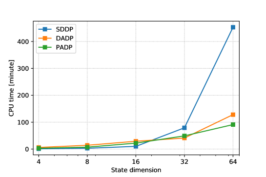
Figure 1: CPU time for the three algorithms as a function of the state dimension

4.3.2 Quality of the Theoretical Bounds

In Table 3, we give the lower and upper bounds (of the optimal cost $V_{0}(x_{0})$ of the global optimization problem) achieved by the three algorithms (SDDP, DADP, PADP).

We recall that SDDP returns a lower bound of the optimal cost $V_{0}(x_{0})$, both by nature and also because we used a suitable resampling of the global uncertainty distribution instead of the original distribution itself (see the discussion in §4.2). DADP and PADP lower and upper bounds are given by Equation (21) and Equation (22) respectively. In Table 3, we observe that

• SDDP’s and DADP’s lower bounds are close to each other,

• for problems with more than 12 nodes, DADP’s lower bound is up to 2.6% better than SDDP’s lower bound,

• the gap between PADP’s upper bound and the two lower bounds is rather large.

Problem	3-nodes	6-nodes	12-nodes	24-nodes	48-nodes
SDDP LB	225.2	455.9	889.7	1752.8	3310.3
DADP LB	213.7	447.3	896.7	1787.0	3396.4
PADP UB	252.1	528.5	1052.3	2100.7	4016.6

Table 3: Upper and lower bounds (of the optimal cost $V_{0}(x_{0})$ of the global optimization problem) given by SDDP, DADP and PADP

To sum up, DADP achieves a slightly better lower bound than SDDP, with much less CPU time (and a parallel version of DADP would give even better performance in terms of CPU time).

4.3.3 Policy Simulation Performances

In Table 4, we give the performances of the policies yielded by the three algorithms. The SDDP, DADP and PADP values are obtained by Monte Carlo simulation of the corresponding policies on $5,000$ scenarios. The notation $\pm$ corresponds to the 95% confidence interval for the numerical evaluation of the expected costs. We use the value obtained by the SDDP policy as a reference, a positive gap meaning that the corresponding policy makes better than the SDDP policy. All these values are statistical upper bounds of the optimal cost $V_{0}(x_{0})$ of the global optimization problem.

Network	3-nodes	6-nodes	12-nodes	24-nodes	48-nodes
SDDP value	226 $\pm$ 0.6	471 $\pm$ 0.8	936 $\pm$ 1.1	1859 $\pm$ 1.6	3550 $\pm$ 2.3
DADP value	228 $\pm$ 0.6	464 $\pm$ 0.8	923 $\pm$ 1.2	1839 $\pm$ 1.6	3490 $\pm$ 2.3
Gap	- 0.8 %	+ 1.5 %	+1.4%	+1.1%	+1.7%
PADP value	229 $\pm$ 0.6	471 $\pm$ 0.8	931 $\pm$ 1.1	1856 $\pm$ 1.6	3508 $\pm$ 2.2
Gap	-1.3%	0.0%	+0.5%	+0.2%	+1.2%

Table 4: Simulation costs (Monte Carlo) for policies induced by SDDP, DADP and PADP

We make the following observations:

• for problems with more than 6 nodes, both the DADP policy and the PADP policy beat the SDDP policy,

• the DADP policy gives better results than the PADP policy,

• comparing with the last line of Table 3, the statistical upper bounds are much closer to SDDP and DADP lower bounds than PADP’s exact upper bound.

For this last observation, our interpretation is as follows: the PADP algorithm is penalized because, as the resource coordination process is deterministic, it imposes constant importation flows for every possible realization of the uncertainties (see also the interpretation of PADP in the case of a decentralized information structure in §3.4).

5 Conclusions

We have considered multistage stochastic optimization problems involving multiple units coupled by spatial static constraints. We have presented a formalism for joint temporal and spatial decomposition. We have provided two fully parallelizable algorithms that yield theoretical bounds, value functions and admissible policies. We have stressed the key role played by information structures in the performance of the decomposition schemes. We have tested these algorithms on the management of several district microgrids. Numerical results have showed the effectiveness of the approach: the price decomposition algorithm beats the reference SDDP algorithm for large-scale problems with more than 12 nodes, both in terms of theoretical bounds and policy performance, and in terms of computation time. On problems with up to 48 nodes (corresponding to 64 state variables), we have observed that their performance scales well as the dimension of the state grew: SDDP is affected by the well-known curse of dimensionality, whereas decomposition-based methods are not.

Possible extensions are the following. In §3.2 and in §3.3, we have presented a serial version of the decomposition algorithms, but we believe that leveraging their parallel nature could decrease further their computation time. In §3.1, we have only considered deterministic price and resource coordination processes. Using larger search sets for the coordination variables, e.g. considering Markovian coordination processes, would make it possible to improve the performance of the algorithms (see [13, Chap. 7] for further details). However, one would need to analyze how to obtain a good trade-off between accuracy and numerical performance.

References

• [1] Léonard Bacaud, Claude Lemaréchal, Arnaud Renaud, and Claudia Sagastizábal. Bundle methods in stochastic optimal power management: A disaggregated approach using preconditioners. Computational Optimization and Applications, 20(3):227–244, 2001.
• [2] Kengy Barty, Pierre Carpentier, and Pierre Girardeau. Decomposition of large-scale stochastic optimal control problems. RAIRO-Operations Research, 44(3):167–183, 2010.
• [3] Richard Bellman. Dynamic Programming. Princeton University Press, New Jersey, 1957.
• [4] D. P. Bertsekas and S. E. Shreve. Stochastic Optimal Control: The Discrete-Time Case. Athena Scientific, Belmont, Massachusets, 1996.
• [5] Dimitri P. Bertsekas. Dynamic programming and optimal control, volume 1. Athena Scientific Belmont, MA, third edition, 2005.
• [6] P. Carpentier, J.-Ph. Chancelier, V. Leclère, and F. Pacaud. Stochastic decomposition applied to large-scale hydro valleys management. European Journal of Operational Research, 270(3):1086–1098, 2018.
• [7] Pierre Carpentier, Jean-Philippe Chancelier, Guy Cohen, and Michel De Lara. Stochastic Multi-Stage Optimization, volume 75. Springer, 2015.
• [8] Pierre Carpentier and Guy Cohen. Décomposition-coordination en optimisation déterministe et stochastique, volume 81. Springer, 2017.
• [9] G. Cohen. Auxiliary Problem Principle and decomposition of optimization problems. Journal of Optimization Theory and Applications, 32(3):277–305, 11 1980.
• [10] Pierre Girardeau, Vincent Leclère, and Andrew B. Philpott. On the convergence of decomposition methods for multistage stochastic convex programs. Mathematics of Operations Research, 40(1):130–145, 2014.
• [11] Kibaek Kim and Victor M Zavala. Algorithmic innovations and software for the dual decomposition method applied to stochastic mixed-integer programs. Mathematical Programming Computation, pages 1–42, 2018.
• [12] Nils Löhndorf and Alexander Shapiro. Modeling time-dependent randomness in stochastic dual dynamic programming. European Journal of Operational Research, 273(2):650–671, 2019.
• [13] François Pacaud. Decentralized Optimization Methods for Efficient Energy Management under Stochasticity. Thèse de doctorat, Université Paris-Est, 2018.
• [14] R Tyrrell Rockafellar. Conjugate duality and optimization, volume 16. Siam, 1974.
• [15] R Tyrrell Rockafellar and Roger J-B Wets. Scenarios and policy aggregation in optimization under uncertainty. Mathematics of operations research, 16(1):119–147, 1991.
• [16] Napat Rujeerapaiboon, Kilian Schindler, Daniel Kuhn, and Wolfram Wiesemann. Scenario reduction revisited: Fundamental limits and guarantees. Mathematical Programming, pages 1–36, 2018.
• [17] Andrzej Ruszczyński. Decomposition methods in stochastic programming. Mathematical programming, 79(1):333–353, 1997.
• [18] Alexander Shapiro, Wajdi Tekaya, Joari P da Costa, and Murilo P Soares. Final report for technical cooperation between Georgia Institute of Technology and ONS – Operador Nacional do Sistema Elétrico. Georgia Tech ISyE Report, 2012.
• [19] Andreas Wächter and Lorenz T Biegler. On the implementation of an interior-point filter line-search algorithm for large-scale nonlinear programming. Mathematical programming, 106(1):25–57, 2006.
• [20] Jean-Paul Watson and David L Woodruff. Progressive hedging innovations for a class of stochastic mixed-integer resource allocation problems. Computational Management Science, 8(4):355–370, 2011.