Upper and Lower Bounds for Large Scale Multistage Stochastic Optimization Problems: Application to Microgrid Management

Abstract

We consider a microgrid where different prosumers exchange energy altogether by the edges of a given network. Each prosumer is located to a node of the network and encompasses energy consumption, energy production and storage capacities (battery, electrical hot water tank). The problem is coupled both in time and in space, so that a direct resolution of the problem for large microgrids is out of reach (curse of dimensionality). By affecting price or resources to each node in the network and resolving each nodal subproblem independently by Dynamic Programming, we provide decomposition algorithms that allow to compute a set of decomposed local value functions in a parallel manner. By summing the local value functions together, we are able, on the one hand, to obtain upper and lower bounds for the optimal value of the problem, and, on the other hand, to design global admissible policies for the original system. Numerical experiments are conducted on microgrids of different size, derived from data given by the research and development centre Efficacity, dedicated to urban energy transition. These experiments show that the decomposition algorithms give better results than the standard SDDP method, both in terms of bounds and policy values. Moreover, the decomposition methods are much faster than the SDDP method in terms of computation time, thus allowing to tackle problem instances incorporating more than 60 state variables in a Dynamic Programming framework.

1 Introduction

Multistage stochastic optimization problems are, by essence, complex because their solutions are indexed both by stages (time) and by uncertainties (scenarios). Hence, their large scale nature makes decomposition methods appealing. We refer to (ruszczynski1997decomposition, ) and (carpentier2017decomposition, ) for a generic description of decomposition methods in stochastic programming problems. Dynamic Programming methods and their extensions are temporal decomposition methods, that have been used on a wide panel of problems, for example in dam management (shapiro2012final, ). Spatial decomposition of large-scale optimization problems was first studied in cohen80 , and extended to open-loop stochastic optimization problems (cohenculioli90, ). Recent developments have mixed spatial decomposition methods with Dynamic Programming to effectively solve large scale multistage stochastic optimization problems. This work led to the introduction of the so-called Dual Approximate Dynamic Programming (DADP) algorithm, which was first applied to unit-commitment problems with a single central coupling constraint linking different stocks altogether (barty2010decomposition, ). We have extended this kind of methods in the companion paper (bounds2019theory, ), on the one hand by considering general coupling constraints among units, and, on the other hand, by using two different decomposition schemes, namely, price and resource decompositions. This article presents applications of price and resource decomposition schemes to the energy management of large scale urban microgrids.

General coupling constraints often arise from flows conservation on a graph. Optimization problems on graphs (monotropic optimization) have been studied since long (rockafellar1984network, ; bertsekas2008extended, ), with applications, for example, to solve network utility problems formulated as two-stage stochastic optimization problems (chatzipanagiotis2015augmented, ). Our motivation rather comes from electrical microgrid management, where buildings (units) are able to consume, produce and store energy and are interconnected through a network. A broad overview of the emergence of consumer-centric electricity markets is given in pinson2018emergence . We suppose here that all actors are benevolent, allowing a central planner to coordinate the local units between each other. Each local unit includes storages (hot water tank and possibly a battery), and has to satisfy heat and electrical demands. It also has the possibility to import energy from an external regional grid if needed. Some local units (prosumers) are able to produce their own energy with solar panels, so as to satisfy their needs and export the surplus to other consumers. The exchanges through the network are modeled as a network flow problem on a graph. We suppose that the system is impacted by uncertainties, both in production (e.g. solar panels) or in demand (e.g. electrical demands). Thus, the global problem can naturally be formulated as a sum of local multistage stochastic optimization subproblems coupled together via a global network constraint. Such problems have been studied in thesepacaud . They are specially challenging from the dynamic optimization point of view since the number of buildings may be large in a district. We address districts with up to 48 buildings (with 64 associated state variables), that is, a size largely beyond the limits imposed by the well-known curse of dimensionality faced by Dynamic Programming. The data associated with the districts we are studying have been provided by Efficacity. The local solar energy productions match realistic data corresponding to a summer day in Paris. The local demands are generated using a stochastic simulator experimentally validated schutz2015comparison . Efficacity is the urban Energy Transition Institute (ITE), established in 2014 with the French government support. The aim of Efficacity is to develop and implement innovative solutions to build an energy-efficient and massively carbon-efficient city.

The paper is organized as follows. In Sect. 2, we model the global optimization problem associated with a microgrid and apply to it the main results obtained in the companion paper bounds2019theory . We present both price and resource decomposition schemes and recall how the Bellman functions of the global problem are bounded above (resp. below) by the sum of local resource-decomposed (resp. price decomposed) value functions that satisfy recursive Dynamic Programming equations. In Sect. 3, we present numerical results for different microgrids of increasing size and complexity. We compare the two decomposition algorithms with a state of the art Stochastic Dual Dynamic Programming (SDDP) algorithm. We analyse the convergence of all algorithms, and we compute the bounds obtained by all algorithms. Thanks to the Bellman functions computed by all algorithms, we are able to devise online policies for the initial optimization problem and we compare the associated expected costs. The analysis of case studies consisting of district microgrids coupling up to 48 buildings together enlightens that decomposition methods give better results in terms of economic performance, and achieve up to a 4 times speedup in terms of computational time.

2 Optimal management of a district microgrid

In this section, we write the optimization problem corresponding to a district microgrid energy management system on a graph in §2.1. We detail how to decompose the problem node by node in §2.2, both by using price and resource decomposition. In §2.3, we show how to find the most appropriate deterministic price and resource processes for obtaining the best possible upper and lower bounds.

2.1 Global optimization problem

A district microgrid is represented by a directed graph $G=(\mathcal{V},\mathcal{E})$, with $\mathcal{V}$ the set of nodes and $\mathcal{E}$ the set of edges. We denote by $N_{\mathcal{V}}$ the number of nodes, and by $N_{\mathcal{E}}$ the number of edges. Each node of the graph corresponds to a single building comprising stocks, energy production and local consumption. These buildings exchange energy through the edges of the graph.

We first detail the different flows occurring in the graph and the coupling constraints existing between flows in edges and flows at nodes. We then formulate at each node a local multistage stochastic optimization subproblem, as well as a transportation subproblem on the graph. Finally, we gather the coupling constraints and the subproblems inside a global optimization problem.

2.1.1 Exchanging flows through edges

Flows are transported through the graph via the edges, each edge $e\in\llbracket 1,N_{\mathcal{E}}\rrbracket$ transporting a flow $q^{e}$ and each node $i\in\llbracket 1,N_{\mathcal{V}}\rrbracket$ importing or exporting a flow $f^{i}$. Here $\llbracket 1,N\rrbracket=\{1,2,\cdots,N\}$ denotes the set of integers between 1 and $N$.

The node flows $f^{i}$ and the edge flows $q^{e}$ are related via a balance equation (Kirchhoff’s current law), which states that the sum of the algebraic edge flows arriving at a particular node $i$ is equal to the node flow $f^{i}$. The Kirchhoff’s current law can be written in matrix form as

$$Aq+f=0\;,$$ (1)

where $f=(f^{1},\cdots,f^{N_{\mathcal{V}}})^{\top}$ is the vector of node flows, $q=(q^{1},\cdots,q^{N_{\mathcal{E}}})^{\top}$ is the vector of edge flows and where $A\in\mathbb{R}^{N_{\mathcal{V}}\times N_{\mathcal{E}}}$ is the node-edge incidence matrix of the graph $G=(\mathcal{V},\mathcal{E})$. Column $e$ of $A$ represents the edge $e$ of the directed graph, with values $+1$ (resp. $-1$) at the initial (resp. final) node of the arc, and $0$ elsewhere.

2.1.2 Production cost on each node

Each node of the graph $G$ corresponds to a building which may comprise stocks (hot water tank, battery), production (solar panel), electric consumption. In case that the local production cannot satisfy the local demand, external energy is bought to the regional grid. We denote by $T$ the time horizon, by $\{0,1,\dots,T\}$ the discrete time span (in the application described in §3.1, a unit period represents a 15mn time step). We write out all random variables in bold. For a node $i\in\llbracket 1,N_{\mathcal{V}}\rrbracket$, the nodal subproblem is the minimization of a functional $J_{\mathcal{V}}^{i}(\boldsymbol{F^{\textstyle\text{\unboldmath$\scriptstyle i$}}_{\textstyle\text{\unboldmath$\scriptstyle$}}},x_{0}^{i})$ depending on the node flow process $\boldsymbol{F^{\textstyle\text{\unboldmath$\scriptstyle i$}}_{\textstyle\text{\unboldmath$\scriptstyle$}}}=(\boldsymbol{F^{\textstyle\text{\unboldmath$\scriptstyle i$}}_{\textstyle\text{\unboldmath$\scriptstyle 0$}}},\cdots,\boldsymbol{F^{\textstyle\text{\unboldmath$\scriptstyle i$}}_{\textstyle\text{\unboldmath$\scriptstyle T-1$}}})^{\top}$ arriving at node $i$ between times $0$ and $T-1$.

Let $\{\mathbb{X}_{t}^{i}\}_{t\in\llbracket 0,T\rrbracket}$, $\{\mathbb{U}_{t}^{i}\}_{t\in\llbracket 0,T-1\rrbracket}$ and $\{\mathbb{W}_{t}^{i}\}_{t\in\llbracket 1,T\rrbracket}$ be sequences of Euclidian spaces of type $\mathbb{R}^{p}$, with appropriate dimensions $p$ (possibly depending on time $t$ and node $i$). The optimal nodal cost $J_{\mathcal{V}}^{i}$ is given by

$$J_{\mathcal{V}}^{i}(\boldsymbol{F^{\textstyle\text{\unboldmath$\scriptstyle i$}}_{\textstyle\text{\unboldmath$\scriptstyle$}}},x_{0}^{i})=\min_{\boldsymbol{X}^{i},\boldsymbol{U}^{i}}\; \mathbb{E}\bigg{[}\sum_{t=0}^{T-1}L^{i}_{t}(\boldsymbol{X^{\textstyle\text{\unboldmath$\scriptstyle i$}}_{\textstyle\text{\unboldmath$\scriptstyle t$}}},\boldsymbol{U^{\textstyle\text{\unboldmath$\scriptstyle i$}}_{\textstyle\text{\unboldmath$\scriptstyle t$}}},\boldsymbol{W^{\textstyle\text{\unboldmath$\scriptstyle i$}}_{\textstyle\text{\unboldmath$\scriptstyle t+1$}}})+K^{i}(\boldsymbol{X}_{T}^{i})\bigg{]}\;,$$ (2a)

$$\text{s.t.}\ \forall t\in\llbracket 0,T\!-\!1\rrbracket \boldsymbol{X}_{t+1}^{i}={g}_{t}^{i}(\boldsymbol{X}^{i}_{t},\boldsymbol{U}_{t}^{i},\boldsymbol{W}_{t+1}^{i})\;,\enspace\boldsymbol{X}_{0}^{i}=x_{0}^{i}\;,$$ (2b)

$$\Delta_{t}^{i}(\boldsymbol{X}_{t}^{i},\boldsymbol{U}_{t}^{i},\boldsymbol{W}_{t+1}^{i})=\boldsymbol{F^{\textstyle\text{\unboldmath$\scriptstyle i$}}_{\textstyle\text{\unboldmath$\scriptstyle t$}}}\;,$$ (2c)

$$\sigma(\boldsymbol{U}_{t}^{i})\subset\sigma(\boldsymbol{W}_{1},\cdots,\boldsymbol{W}_{t},\boldsymbol{W}_{t+1})\;,$$ (2d)

where we denote by $\boldsymbol{X}^{i}=(\boldsymbol{X}^{i}_{0},\cdots,\boldsymbol{X}^{i}_{T})$, $\boldsymbol{U}^{i}=(\boldsymbol{U}^{i}_{0},\cdots,\boldsymbol{U}^{i}_{T-1})$ and $\boldsymbol{W}^{i}=(\boldsymbol{W}^{i}_{0},\cdots,\boldsymbol{W}^{i}_{T})$ the local state (stocks), control (production) and uncertainty (consumption) processes. Constraint (2c) represents the energy balance inside node $i$ for each time $t$, with $\Delta_{t}^{i}:\mathbb{X}_{t}^{i}\times\mathbb{U}_{t}^{i}\times\mathbb{W}_{t+1}^{i}\rightarrow\mathbb{R}$. In order to be able to almost surely satisfy Constraints (2c), we assume that all decisions follow the hazard-decision information structure, that is, decision $\boldsymbol{U}_{t}^{i}$ is taken after noise $\boldsymbol{W}_{t+1}$ has been observed, hence the specific form of Constraint (2d). This slightly differs from the scope presented in the companion paper bounds2019theory where the decision-hazard information structure was considered, but does not change the kind of results already obtained.

We detail the dynamics (2b) in building $i$. A battery is modeled with the linear dynamics

$$\boldsymbol{B^{\textstyle\text{\unboldmath$\scriptstyle i$}}_{\textstyle\text{\unboldmath$\scriptstyle{t+1}$}}}=\alpha_{b}\boldsymbol{B^{\textstyle\text{\unboldmath$\scriptstyle i$}}_{\textstyle\text{\unboldmath$\scriptstyle t$}}}+\Delta T\big{(}\rho_{c}(\boldsymbol{U^{\textstyle\text{\unboldmath$\scriptstyle b,i$}}_{\textstyle\text{\unboldmath$\scriptstyle t$}}})^{+}-\dfrac{1}{\rho_{d}}(\boldsymbol{U^{\textstyle\text{\unboldmath$\scriptstyle b,i$}}_{\textstyle\text{\unboldmath$\scriptstyle t$}}})^{-}\big{)}\;,\enspace\forall t\in\llbracket 0,\dots,T-1\rrbracket\;,$$ (3a)

where $$\boldsymbol{B^{\textstyle\text{\unboldmath$\scriptstyle i$}}_{\textstyle\text{\unboldmath$\scriptstyle t$}}} t \boldsymbol{U}_{t}^{b,i} \alpha_{b} (\rho_{d},\rho_{c})$$ is the energy stored inside the battery at time , is the power exchanged with the battery, is the auto-discharge rate and are given yields. An electrical hot water tanks is modeled with the linear dynamics

$$\boldsymbol{H^{\textstyle\text{\unboldmath$\scriptstyle i$}}_{\textstyle\text{\unboldmath$\scriptstyle{t+1}$}}}=\alpha_{h}\boldsymbol{H^{\textstyle\text{\unboldmath$\scriptstyle i$}}_{\textstyle\text{\unboldmath$\scriptstyle t$}}}+\Delta T\big{(}\beta_{h}\boldsymbol{U}_{t}^{t,i}-\boldsymbol{D^{\textstyle\text{\unboldmath$\scriptstyle hw,i$}}_{\textstyle\text{\unboldmath$\scriptstyle{t+1}$}}}\big{)}\;,\enspace\forall t\in\llbracket 0,..,T-1\rrbracket\;,$$ (3b)

where $$\boldsymbol{H^{\textstyle\text{\unboldmath$\scriptstyle i$}}_{\textstyle\text{\unboldmath$\scriptstyle t$}}} t \boldsymbol{U}_{t}^{t,i} \boldsymbol{D^{\textstyle\text{\unboldmath$\scriptstyle hw,i$}}_{\textstyle\text{\unboldmath$\scriptstyle{t+1}$}}} t t+1 \alpha_{h} \beta_{h}$$ is the energy stored inside the tank at time , is the power used to heat the tank, is the domestic hot water demand between time and . The coefficient is a discharge rate corresponding to the losses by conduction and is a conversion coefficient.

Depending on the possible presence of a battery inside the building, the nodal state $\boldsymbol{X}_{t}^{i}$ has dimension 2 or 1. If node $i$ has a battery, its state is $\boldsymbol{X}_{t}^{i}=(\boldsymbol{B^{\textstyle\text{\unboldmath$\scriptstyle i$}}_{\textstyle\text{\unboldmath$\scriptstyle t$}}},\boldsymbol{H^{\textstyle\text{\unboldmath$\scriptstyle i$}}_{\textstyle\text{\unboldmath$\scriptstyle t$}}})$; otherwise, its state is $\boldsymbol{X}_{t}^{i}=\boldsymbol{H^{\textstyle\text{\unboldmath$\scriptstyle i$}}_{\textstyle\text{\unboldmath$\scriptstyle t$}}}$. The value of the state at time $0$ is known, equal to $x_{0}^{i}$.

Equation (2c) is the node balance at node $i$, with mapping $\Delta_{t}^{i}$ given by

$$\Delta_{t}^{i}(\boldsymbol{X}_{t}^{i},\boldsymbol{U}_{t}^{i},\boldsymbol{W}_{t+1}^{i})=\boldsymbol{U}_{t}^{ne,i}-\boldsymbol{D^{\textstyle\text{\unboldmath$\scriptstyle el,i$}}_{\textstyle\text{\unboldmath$\scriptstyle{t+1}$}}}-\boldsymbol{U}_{t}^{b,i}-\boldsymbol{U}_{t}^{t,i}\;,$$ (4)

$\boldsymbol{D^{\textstyle\text{\unboldmath$\scriptstyle el,i$}}_{\textstyle\text{\unboldmath$\scriptstyle{t+1}$}}}$ being the residual electricity demand between time $t$ and $t+1$, and $\boldsymbol{U}_{t}^{ne,i}$ being the amount of electricity taken from the external national grid.

Collecting the different variables involved in the model, the control variable for building $i$ is $\boldsymbol{U}_{t}^{i}=(\boldsymbol{U}_{t}^{b,i},\boldsymbol{U}_{t}^{t,i},\boldsymbol{U}_{t}^{ne,i})$ and the noise variable affecting node $i$ is $\boldsymbol{W}_{t+1}^{i}=(\boldsymbol{D^{\textstyle\text{\unboldmath$\scriptstyle hw,i$}}_{\textstyle\text{\unboldmath$\scriptstyle{t+1}$}}},\boldsymbol{D^{\textstyle\text{\unboldmath$\scriptstyle el,i$}}_{\textstyle\text{\unboldmath$\scriptstyle{t+1}$}}})$.

The cost function at node $i$ in (2a) depends linearly on the price $p_{t}^{el}$ to import electricity from the external national grid, so that

$$L^{i}_{t}(\boldsymbol{X^{\textstyle\text{\unboldmath$\scriptstyle i$}}_{\textstyle\text{\unboldmath$\scriptstyle t$}}},\boldsymbol{U^{\textstyle\text{\unboldmath$\scriptstyle i$}}_{\textstyle\text{\unboldmath$\scriptstyle t$}}},\boldsymbol{W^{\textstyle\text{\unboldmath$\scriptstyle i$}}_{\textstyle\text{\unboldmath$\scriptstyle t+1$}}})=p_{t}^{el}\boldsymbol{U}_{t}^{ne,i}\;.$$ (5)

The final cost $K^{i}$ is a penalization to avoid an empty electrical hot water tank at the end of the day.

The global nodal cost $J_{\mathcal{V}}\big{(}\boldsymbol{F^{\textstyle\text{\unboldmath$\scriptstyle$}}_{\textstyle\text{\unboldmath$\scriptstyle$}}},(x_{0}^{1},\ldots,x_{0}^{N_{\mathcal{V}}})\big{)}$ over the whole network is obtained by summing the local nodal costs

$$J_{\mathcal{V}}\big{(}\boldsymbol{F^{\textstyle\text{\unboldmath$\scriptstyle$}}_{\textstyle\text{\unboldmath$\scriptstyle$}}},(x_{0}^{1},\ldots,x_{0}^{N_{\mathcal{V}}})\big{)}=\sum_{i=1}^{N_{\mathcal{V}}}J_{\mathcal{V}}^{i}(\boldsymbol{F^{\textstyle\text{\unboldmath$\scriptstyle i$}}_{\textstyle\text{\unboldmath$\scriptstyle$}}},x_{0}^{i})\;.$$ (6)

2.1.3 Transportation cost on edges

We now consider the edge costs arising when transporting the flow $\boldsymbol{Q^{\textstyle\text{\unboldmath$\scriptstyle e$}}_{\textstyle\text{\unboldmath$\scriptstyle t$}}}$ through each edge $e\in\llbracket 1,N_{\mathcal{E}}\rrbracket$ and for any time $t\in\llbracket 0,T-1\rrbracket$. The global edge cost $J_{\mathcal{E}}(\boldsymbol{Q^{\textstyle\text{\unboldmath$\scriptstyle$}}_{\textstyle\text{\unboldmath$\scriptstyle$}}})$ aggregates all transport costs through the different edges in the graph, namely

$$J_{\mathcal{E}}(\boldsymbol{Q^{\textstyle\text{\unboldmath$\scriptstyle$}}_{\textstyle\text{\unboldmath$\scriptstyle$}}})=\mathbb{E}\bigg{[}\sum_{e=1}^{N_{\mathcal{E}}}\sum_{t=0}^{T-1}l_{t}^{e}(\boldsymbol{Q^{\textstyle\text{\unboldmath$\scriptstyle e$}}_{\textstyle\text{\unboldmath$\scriptstyle t$}}})\bigg{]}\;,$$ (7)

where $l_{t}^{e}:\mathbb{R}\rightarrow\mathbb{R}$ are convex real valued functions assumed to be “easy to compute”, e.g. quadratic. The cost $l_{t}^{e}$ can be induced by a difference in pricing, a fixed toll between the different nodes, or by the energy losses through the network.

The global edge cost function $J_{\mathcal{E}}$ in (7) is additive and thus decomposable w.r.t. (with respect to) time and edges.

2.1.4 Global optimization problem

We have stated local nodal criteria (2) and a global edge criterion (7), both depending on node and edge flows coupled by Constraint (1) at each time $t\in\llbracket 0,T-1\rrbracket$, that is, $A\boldsymbol{Q^{\textstyle\text{\unboldmath$\scriptstyle$}}_{\textstyle\text{\unboldmath$\scriptstyle t$}}}+\boldsymbol{F^{\textstyle\text{\unboldmath$\scriptstyle$}}_{\textstyle\text{\unboldmath$\scriptstyle t$}}}=0$. We rewrite these constraints in a single constraint involving the global node flow and edge flow processes: $\mathcal{A}\boldsymbol{Q^{\textstyle\text{\unboldmath$\scriptstyle$}}_{\textstyle\text{\unboldmath$\scriptstyle$}}}+\boldsymbol{F^{\textstyle\text{\unboldmath$\scriptstyle$}}_{\textstyle\text{\unboldmath$\scriptstyle$}}}=0$. The matrix $\mathcal{A}\in\mathbb{R}^{T.N_{\mathcal{V}}\times T.N_{\mathcal{E}}}$ is a block-diagonal matrix with matrix $A$ as diagonal element. We are now able to formulate a global optimization problem as

$$V_{0}^{\sharp}(x_{0}^{1},\cdots,x_{0}^{N_{\mathcal{V}}})=\min_{\boldsymbol{F^{\textstyle\text{\unboldmath$\scriptstyle$}}_{\textstyle\text{\unboldmath$\scriptstyle$}}},\boldsymbol{Q^{\textstyle\text{\unboldmath$\scriptstyle$}}_{\textstyle\text{\unboldmath$\scriptstyle$}}}}\; \sum_{i=1}^{N_{\mathcal{V}}}J_{\mathcal{V}}^{i}(\boldsymbol{F^{\textstyle\text{\unboldmath$\scriptstyle i$}}_{\textstyle\text{\unboldmath$\scriptstyle$}}},x_{0}^{i})+J_{\mathcal{E}}(\boldsymbol{Q^{\textstyle\text{\unboldmath$\scriptstyle$}}_{\textstyle\text{\unboldmath$\scriptstyle$}}})$$ (8a)

s.t. $$\mathcal{A}\boldsymbol{Q^{\textstyle\text{\unboldmath$\scriptstyle$}}_{\textstyle\text{\unboldmath$\scriptstyle$}}}+\boldsymbol{F^{\textstyle\text{\unboldmath$\scriptstyle$}}_{\textstyle\text{\unboldmath$\scriptstyle$}}}=0\;.$$ (8b)

Problem (8) couples $N_{\mathcal{V}}+1$ independent criteria through Constraint (8b). As the resulting criterion is additive and Constraint (8b) is affine, Problem (8) has a nice form to use decomposition-coordination methods.

Remark 1.

There may be additional constraints in the problem, for example bound constraints $\underline{F}_{t}^{i}\leq\boldsymbol{F^{\textstyle\text{\unboldmath$\scriptstyle i$}}_{\textstyle\text{\unboldmath$\scriptstyle t$}}}\leq\overline{F}_{t}^{i}$ on the node flows, and bound constraints $\underline{Q}_{t}^{e}\leq\boldsymbol{Q^{\textstyle\text{\unboldmath$\scriptstyle e$}}_{\textstyle\text{\unboldmath$\scriptstyle t$}}}\leq\overline{Q}_{t}^{e}$. on the edge flows. These constraints may be modeled, in the global optimization problem criterion, by additional terms like

$$\mathbb{E}\bigg{[}\sum_{i=1}^{N_{\mathcal{V}}}\mathbb{I}_{[\underline{F}_{t}^{i},\overline{F}_{t}^{i}]^{T}}(\boldsymbol{F^{\textstyle\text{\unboldmath$\scriptstyle i$}}_{\textstyle\text{\unboldmath$\scriptstyle$}}})\bigg{]}+\mathbb{E}\bigg{[}\sum_{e=1}^{N_{\mathcal{E}}}\sum_{t=0}^{T-1}\mathbb{I}_{[\underline{Q}_{t}^{e},\overline{Q}_{t}^{e}]}(\boldsymbol{Q^{\textstyle\text{\unboldmath$\scriptstyle e$}}_{\textstyle\text{\unboldmath$\scriptstyle t$}}})\bigg{]}\;,$$

where

$$\mathbb{I}_{E}:x\mapsto\left\{\begin{aligned} 0\quad&\text{ if }x\in E\\ +\infty&\text{ otherwise}\end{aligned}\right.$$

is the indicator function of the set $E$. These additional terms do not change the additive structure of the cost function.

2.2 Mixing nodal and time decomposition on a microgrid

In the companion paper bounds2019theory , we introduced a generic framework to bound a global problem by decomposing it into smaller local subproblems, easier to solve. In Problem (8), the coupling constraints (8b) can be written $(\boldsymbol{F^{\textstyle\text{\unboldmath$\scriptstyle$}}_{\textstyle\text{\unboldmath$\scriptstyle$}}},\boldsymbol{Q^{\textstyle\text{\unboldmath$\scriptstyle$}}_{\textstyle\text{\unboldmath$\scriptstyle$}}})\in-S$, where the convex set $S$ of $\mathbb{R}^{T\cdot N_{\mathcal{V}}}\times\mathbb{R}^{T\cdot N_{\mathcal{E}}}$ is the linear subspace

$$S=\big{\{}(f,q)\in\mathbb{R}^{T\cdot N_{\mathcal{V}}}\times\mathbb{R}^{T\cdot N_{\mathcal{E}}}\;\big{|}\;\mathcal{A}q+f=0\big{\}}\;.$$ (9)

Problem (8) lies in the generic framework introduced in bounds2019theory , and the coupling equation $\mathcal{A}\boldsymbol{Q^{\textstyle\text{\unboldmath$\scriptstyle$}}_{\textstyle\text{\unboldmath$\scriptstyle$}}}+\boldsymbol{F^{\textstyle\text{\unboldmath$\scriptstyle$}}_{\textstyle\text{\unboldmath$\scriptstyle$}}}=0$ becomes a special case of the generic coupling constraint of this framework. Moreover, it can easily be checked that the dual cone of the set $S$ defined in (9) has the following expression:

$$S^{\star}=\big{\{}(p,\mu)\in\mathbb{R}^{T\cdot N_{\mathcal{V}}}\times\mathbb{R}^{T\cdot N_{\mathcal{E}}}\;\big{|}\;\mathcal{A}^{\top}p-\mu=0\big{\}}\;.$$ (10)

The duality terms arising from Constraint (8b) are given by the formula

$$\big{\langle}p\>,f\big{\rangle}+\big{\langle}\mu\>,q\big{\rangle}=\big{\langle}p\>,(\mathcal{A}q+f)\big{\rangle}\;,\enspace\forall(f,q)\in S\;,\enspace\forall(p,\mu)\in S^{\star}\;,$$ (11)

where $(u,v)\mapsto\big{\langle}u\>,v\big{\rangle}$ is the usual scalar product on $\mathbb{R}^{T\cdot N_{\mathcal{V}}}$. In order to solve Problem (8), we apply the decomposition schemes introduced in bounds2019theory . More precisely, we first apply spatial decoupling into nodal and edge subproblems, and then apply the temporal decomposition induced by Dynamic Programming.

2.2.1 Price decomposition of the global problem

We follow the procedure introduced in (bounds2019theory, , §2.2) to provide a lower bound and to solve Problem (8) by price decomposition. We limit ourselves to deterministic price processes, that is, vectors $p=(p^{1},\ldots,p^{N_{\mathcal{V}}})\in\mathbb{R}^{T\cdot N_{\mathcal{V}}}$. By Equation (11), the global price value function associated with Problem (8) has the following expression, for all $x_{0}=(x_{0}^{1},\cdots,x_{0}^{N_{\mathcal{V}}})\in\mathbb{X}_{0}^{1}\times\dots\times\mathbb{X}_{0}^{N_{\mathcal{V}}}$,

$$\underline{V}[p](x_{0})=\min_{\boldsymbol{F^{\textstyle\text{\unboldmath$\scriptstyle$}}_{\textstyle\text{\unboldmath$\scriptstyle$}}},\boldsymbol{Q^{\textstyle\text{\unboldmath$\scriptstyle$}}_{\textstyle\text{\unboldmath$\scriptstyle$}}}}\;\sum_{i=1}^{N_{\mathcal{V}}}J_{\mathcal{V}}^{i}(\boldsymbol{F^{\textstyle\text{\unboldmath$\scriptstyle i$}}_{\textstyle\text{\unboldmath$\scriptstyle$}}},x_{0}^{i})+J_{\mathcal{E}}(\boldsymbol{Q^{\textstyle\text{\unboldmath$\scriptstyle$}}_{\textstyle\text{\unboldmath$\scriptstyle$}}})+\mathbb{E}\big{[}\big{\langle}p\>,\mathcal{A}\boldsymbol{Q^{\textstyle\text{\unboldmath$\scriptstyle$}}_{\textstyle\text{\unboldmath$\scriptstyle$}}}+\boldsymbol{F^{\textstyle\text{\unboldmath$\scriptstyle$}}_{\textstyle\text{\unboldmath$\scriptstyle$}}}\big{\rangle}\big{]}\;.$$ (12)

The global price value function $$\underline{V}[p]$$ naturally decomposes into a sequence of nodal price value functions

$$\underline{V}_{\mathcal{V}}^{i}[p^{i}](x_{0}^{i})=\min_{\boldsymbol{F^{\textstyle\text{\unboldmath$\scriptstyle i$}}_{\textstyle\text{\unboldmath$\scriptstyle$}}}}J_{\mathcal{V}}^{i}(\boldsymbol{F^{\textstyle\text{\unboldmath$\scriptstyle i$}}_{\textstyle\text{\unboldmath$\scriptstyle$}}},x_{0}^{i})+\mathbb{E}\big{[}\big{\langle}p^{i}\>,\boldsymbol{F^{\textstyle\text{\unboldmath$\scriptstyle i$}}_{\textstyle\text{\unboldmath$\scriptstyle$}}}\big{\rangle}\big{]}\;,\enspace\forall i\in\llbracket 1,N_{\mathcal{V}}\rrbracket\;,$$ (13a)

and an edge price value function (which, to the difference of the nodal price value function (13a), does not depend on the initial state $$x_{0}$$)

$$\underline{V}_{\mathcal{E}}[p]=\min_{\boldsymbol{Q^{\textstyle\text{\unboldmath$\scriptstyle$}}_{\textstyle\text{\unboldmath$\scriptstyle$}}}}\;J_{\mathcal{E}}(\boldsymbol{Q^{\textstyle\text{\unboldmath$\scriptstyle$}}_{\textstyle\text{\unboldmath$\scriptstyle$}}})+\mathbb{E}\big{[}\big{\langle}\mathcal{A}^{\top}p\>,\boldsymbol{Q^{\textstyle\text{\unboldmath$\scriptstyle$}}_{\textstyle\text{\unboldmath$\scriptstyle$}}}\big{\rangle}\big{]}\;.$$ (13b)

For all $i\in\llbracket 1,N_{\mathcal{V}}\rrbracket$, considering the expression (2) of the nodal cost $J_{\mathcal{V}}^{i}$, the nodal price value function (13a) is, for $x_{0}^{i}\in\mathbb{X}_{0}^{i}$,

$$\underline{V}_{\mathcal{V}}^{i}[p^{i}](x_{0}^{i})=\min_{\boldsymbol{X}^{i},\boldsymbol{U}^{i},\boldsymbol{F^{\textstyle\text{\unboldmath$\scriptstyle i$}}_{\textstyle\text{\unboldmath$\scriptstyle$}}}}\; \mathbb{E}\bigg{[}\sum_{t=0}^{T-1}\Big{(}L^{i}_{t}(\boldsymbol{X^{\textstyle\text{\unboldmath$\scriptstyle i$}}_{\textstyle\text{\unboldmath$\scriptstyle t$}}},\boldsymbol{U^{\textstyle\text{\unboldmath$\scriptstyle i$}}_{\textstyle\text{\unboldmath$\scriptstyle t$}}},\boldsymbol{W^{\textstyle\text{\unboldmath$\scriptstyle i$}}_{\textstyle\text{\unboldmath$\scriptstyle t+1$}}})+\big{\langle}p_{t}^{i}\>,\boldsymbol{F^{\textstyle\text{\unboldmath$\scriptstyle i$}}_{\textstyle\text{\unboldmath$\scriptstyle t$}}}\big{\rangle}\Big{)}+K^{i}(\boldsymbol{X}_{T}^{i})\bigg{]}\;,$$

s.t. $$\>,\;\forall t\in\llbracket 0,T\!-\!1\rrbracket\;,\enspace$$

$$\boldsymbol{X}_{t+1}^{i}={g}_{t}^{i}(\boldsymbol{X}^{i}_{t},\boldsymbol{U}_{t}^{i},\boldsymbol{W}_{t+1}^{i})\;,\enspace\boldsymbol{X}_{0}^{i}=x_{0}^{i}\;,$$

$$\Delta_{t}^{i}(\boldsymbol{X}_{t}^{i},\boldsymbol{U}_{t}^{i},\boldsymbol{W}_{t+1}^{i})=\boldsymbol{F^{\textstyle\text{\unboldmath$\scriptstyle i$}}_{\textstyle\text{\unboldmath$\scriptstyle t$}}}\;,$$

$$\sigma(\boldsymbol{U}_{t}^{i})\subset\sigma(\boldsymbol{W}_{1},\cdots,\boldsymbol{W}_{t},\boldsymbol{W}_{t+1})\;,$$

The optimal value $\underline{V}_{\mathcal{V}}^{i}[p^{i}](x_{0}^{i})$ can be computed by Dynamic Programming under the so-called white noise assumption.

Assumption 1.

The global uncertainty process $(\boldsymbol{W}_{1},\cdots,\boldsymbol{W}_{T})$ consists of stagewise independent random variables.

For all node $i\in\llbracket 1,N_{\mathcal{V}}\rrbracket$ and price $p^{i}\in\mathbb{R}^{T}$, we introduce the sequence $\{\underline{V}_{{\mathcal{V}},t}^{i}[p^{i}]\}_{t=0,\cdots,T}$ of local price value functions defined, for all $t\in\llbracket 0,T\rrbracket$ and $x_{t}^{i}\in\mathbb{X}_{t}^{i}$, by

$$\underline{V}_{{\mathcal{V}},t}^{i}[p^{i}](x_{t}^{i})=\min_{\boldsymbol{X}^{i},\boldsymbol{U}^{i},\boldsymbol{F^{\textstyle\text{\unboldmath$\scriptstyle i$}}_{\textstyle\text{\unboldmath$\scriptstyle$}}}}\; \mathbb{E}\bigg{[}\sum_{s=t}^{T-1}\Big{(}L^{i}_{s}(\boldsymbol{X^{\textstyle\text{\unboldmath$\scriptstyle i$}}_{\textstyle\text{\unboldmath$\scriptstyle s$}}},\boldsymbol{U^{\textstyle\text{\unboldmath$\scriptstyle i$}}_{\textstyle\text{\unboldmath$\scriptstyle s$}}},\boldsymbol{W^{\textstyle\text{\unboldmath$\scriptstyle i$}}_{\textstyle\text{\unboldmath$\scriptstyle s+1$}}})+\big{\langle}p_{s}^{i}\>,\boldsymbol{F^{\textstyle\text{\unboldmath$\scriptstyle i$}}_{\textstyle\text{\unboldmath$\scriptstyle s$}}}\big{\rangle}\Big{)}+K^{i}(\boldsymbol{X}_{T}^{i})\bigg{]}\;,$$ (14a)

s.t. $$\>,\;\forall t\in\llbracket 0,T\!-\!1\rrbracket\;,\enspace$$

$$\boldsymbol{X}_{s+1}^{i}={g}_{s}^{i}(\boldsymbol{X}^{i}_{s},\boldsymbol{U}_{s}^{i},\boldsymbol{W}_{s+1}^{i})\;,\enspace\boldsymbol{X}_{t}^{i}=x_{t}^{i}\;,$$ (14b)

$$\Delta_{s}^{i}(\boldsymbol{X}_{s}^{i},\boldsymbol{U}_{s}^{i},\boldsymbol{W}_{s+1}^{i})=\boldsymbol{F^{\textstyle\text{\unboldmath$\scriptstyle i$}}_{\textstyle\text{\unboldmath$\scriptstyle s$}}}\;,$$ (14c)

$$\sigma(\boldsymbol{U}_{s}^{i})\subset\sigma(\boldsymbol{W}_{t+1},\cdots,\boldsymbol{W}_{s},\boldsymbol{W}_{s+1})\;,$$ (14d)

with the convention $\underline{V}_{{\mathcal{V}},T}^{i}[p^{i}]=K^{i}$. Under Assumption 1, these local price value functions satisfy the Dynamic Programming equations for all $i\in\llbracket 1,N_{\mathcal{V}}\rrbracket$:

$$\underline{V}_{{\mathcal{V}},T}^{i}[p^{i}](x_{T}^{i}) =K^{i}(x_{T}^{i})\;,$$ (15a)

and, for $$t=T\!-\!1,\ldots,0$$,

$$\underline{V}_{{\mathcal{V}},t}^{i}[p^{i}](x_{t}^{i}) =\mathbb{E}\Big{[}\min_{u_{t}^{i}}L^{i}_{s}(x_{t}^{i},u_{t}^{i},\boldsymbol{W}^{i}_{t})+\big{\langle}p_{t}^{i}\>,\Delta_{t}^{i}(x_{t}^{i},u_{t}^{i},\boldsymbol{W}_{t+1}^{i})\big{\rangle}$$

$$\hskip 93.89418pt+\underline{V}_{{\mathcal{V}},{t+1}}^{i}[p^{i}]\big{(}{g}_{s}^{i}(x_{t}^{i},u_{t}^{i},\boldsymbol{W}_{t+1}^{i})\big{)}\Big{]}\;.$$ (15b)

Note that the measurability constraints $\sigma(\boldsymbol{U}_{t}^{i})\subset\sigma(\boldsymbol{W}_{1},\cdots,\boldsymbol{W}_{t+1})$ in the above problem (14) can be replaced by $\sigma(\boldsymbol{U}_{t}^{i})\subset\sigma(\boldsymbol{W}_{1}^{i},\cdots,\boldsymbol{W}_{t+1}^{i})$ without changing the value $\underline{V}_{\mathcal{V}}^{i}[p^{i}](x_{0}^{i})$. Indeed, Equation (14) only involves the local noise process $(\boldsymbol{W}_{1}^{i},\cdots,\boldsymbol{W}_{T}^{i})$, so that there is no loss of optimality to restrain the measurability of the control process $\boldsymbol{U}^{i}$ to the filtration generated by the local noise process $\boldsymbol{W}^{i}$.

Considering the expression (7) of the edge cost $J_{\mathcal{E}}(\boldsymbol{Q^{\textstyle\text{\unboldmath$\scriptstyle$}}_{\textstyle\text{\unboldmath$\scriptstyle$}}})$, the edge price value function $\underline{V}_{\mathcal{E}}[p]$ is additive w.r.t. time and space, and thus can be decomposed at each time $t$ and each edge $e$. The resulting edge subproblems do not involve any time coupling and can be computed by standard mathematical programming tools or even analytically.

2.2.2 Resource decomposition of the global problem

We now solve Problem (8) by resource decomposition (see (bounds2019theory, , §2.2)) using a deterministic resource process $r=(r^{1},\ldots,r^{N_{\mathcal{V}}})\in\mathbb{R}^{T\cdot N_{\mathcal{V}}}$, such that $r\in\mathrm{im}(\mathcal{A})$. We decompose the global constraint (8b) w.r.t. nodes and edges as

$$\boldsymbol{F^{\textstyle\text{\unboldmath$\scriptstyle$}}_{\textstyle\text{\unboldmath$\scriptstyle$}}}=r\quad,\quad\mathcal{A}\boldsymbol{Q^{\textstyle\text{\unboldmath$\scriptstyle$}}_{\textstyle\text{\unboldmath$\scriptstyle$}}}=-r\;.$$

The global resource value function associated to Problem (8) has the following expression, for all $x_{0}=(x_{0}^{1},\cdots,x_{0}^{N_{\mathcal{V}}})\in\mathbb{X}_{0}^{1}\times\dots\times\mathbb{X}_{0}^{N_{\mathcal{V}}}$,

$$\overline{V}[r](x_{0})=\min_{\boldsymbol{F^{\textstyle\text{\unboldmath$\scriptstyle$}}_{\textstyle\text{\unboldmath$\scriptstyle$}}},\boldsymbol{Q^{\textstyle\text{\unboldmath$\scriptstyle$}}_{\textstyle\text{\unboldmath$\scriptstyle$}}}}\; \sum_{i=1}^{N_{\mathcal{V}}}J_{\mathcal{V}}^{i}(\boldsymbol{F^{\textstyle\text{\unboldmath$\scriptstyle i$}}_{\textstyle\text{\unboldmath$\scriptstyle$}}},x_{0}^{i})+J_{\mathcal{E}}(\boldsymbol{Q^{\textstyle\text{\unboldmath$\scriptstyle$}}_{\textstyle\text{\unboldmath$\scriptstyle$}}})$$ (16a)

s.t. $$\boldsymbol{F^{\textstyle\text{\unboldmath$\scriptstyle$}}_{\textstyle\text{\unboldmath$\scriptstyle$}}}-r=0\;,\enspace\mathcal{A}\boldsymbol{Q^{\textstyle\text{\unboldmath$\scriptstyle$}}_{\textstyle\text{\unboldmath$\scriptstyle$}}}+r=0\;.$$ (16b)

The global resource value function $$\overline{V}[r]$$ naturally decomposes in a sequence of nodal resource value functions

$$\overline{V}_{\mathcal{V}}^{i}[r^{i}](x_{0}^{i})=\min_{\boldsymbol{F^{\textstyle\text{\unboldmath$\scriptstyle i$}}_{\textstyle\text{\unboldmath$\scriptstyle$}}}}\;J_{\mathcal{V}}^{i}(\boldsymbol{F^{\textstyle\text{\unboldmath$\scriptstyle i$}}_{\textstyle\text{\unboldmath$\scriptstyle$}}},x_{0}^{i})\quad\text{s.t.}\quad\boldsymbol{F^{\textstyle\text{\unboldmath$\scriptstyle i$}}_{\textstyle\text{\unboldmath$\scriptstyle$}}}-r^{i}=0\;,\enspace\forall i\in\llbracket 1,N_{\mathcal{V}}\rrbracket\;,$$ (17a)

and an edge resource value function (which does not depend on $$x_{0}$$)

$$\overline{V}_{\mathcal{E}}[r]=\min_{\boldsymbol{Q^{\textstyle\text{\unboldmath$\scriptstyle$}}_{\textstyle\text{\unboldmath$\scriptstyle$}}}}\;J_{\mathcal{E}}(\boldsymbol{Q^{\textstyle\text{\unboldmath$\scriptstyle$}}_{\textstyle\text{\unboldmath$\scriptstyle$}}})\quad\text{s.t.}\quad\mathcal{A}\boldsymbol{Q^{\textstyle\text{\unboldmath$\scriptstyle$}}_{\textstyle\text{\unboldmath$\scriptstyle$}}}+r=0\;.$$ (17b)

For all $i\in\llbracket 1,N_{\mathcal{V}}\rrbracket$, considering the expression (2) of the nodal cost $J_{\mathcal{V}}^{i}$, the nodal resource value function (17a) is, for $x_{0}^{i}\in\mathbb{X}_{0}^{i}$,

$$\overline{V}_{\mathcal{V}}^{i}[r^{i}](x_{0}^{i})=\min_{\boldsymbol{X}^{i},\boldsymbol{U}^{i},\boldsymbol{F^{\textstyle\text{\unboldmath$\scriptstyle i$}}_{\textstyle\text{\unboldmath$\scriptstyle$}}}}\; \mathbb{E}\bigg{[}\sum_{t=0}^{T-1}L^{i}_{t}(\boldsymbol{X^{\textstyle\text{\unboldmath$\scriptstyle i$}}_{\textstyle\text{\unboldmath$\scriptstyle t$}}},\boldsymbol{U^{\textstyle\text{\unboldmath$\scriptstyle i$}}_{\textstyle\text{\unboldmath$\scriptstyle t$}}},\boldsymbol{W^{\textstyle\text{\unboldmath$\scriptstyle i$}}_{\textstyle\text{\unboldmath$\scriptstyle t+1$}}})+K^{i}(\boldsymbol{X}_{T}^{i})\bigg{]}\;,$$

s.t. $$\>,\;\forall t\in\llbracket 0,T\!-\!1\rrbracket\;,\enspace$$

$$\boldsymbol{X}_{t+1}^{i}={g}_{t}^{i}(\boldsymbol{X}^{i}_{t},\boldsymbol{U}_{t}^{i},\boldsymbol{W}_{t+1}^{i})\;,\enspace\boldsymbol{X}_{0}^{i}=x_{0}^{i}\;,$$

$$\Delta_{t}^{i}(\boldsymbol{X}_{t}^{i},\boldsymbol{U}_{t}^{i},\boldsymbol{W}_{t+1}^{i})=\boldsymbol{F^{\textstyle\text{\unboldmath$\scriptstyle i$}}_{\textstyle\text{\unboldmath$\scriptstyle t$}}}\;,$$

$$\sigma(\boldsymbol{U}_{t}^{i})\subset\sigma(\boldsymbol{W}_{1},\cdots,\boldsymbol{W}_{t},\boldsymbol{W}_{t+1})\;,$$

$$\boldsymbol{F^{\textstyle\text{\unboldmath$\scriptstyle i$}}_{\textstyle\text{\unboldmath$\scriptstyle t$}}}-r_{t}^{i}=0\;.$$

If Assumption 1 holds true, $\overline{V}_{\mathcal{V}}^{i}[r^{i}](x_{0}^{i})$ can be computed by Dynamic Programming. That leads to a sequence $\{\overline{V}_{{\mathcal{V}},t}^{i}\}_{t=0,\cdots,T}$ of local resource value functions given, for all $t\in\llbracket 0,T\rrbracket$ and $x_{t}^{i}\in\mathbb{X}_{t}^{i}$, by

$$\overline{V}_{{\mathcal{V}},t}^{i}[r^{i}](x_{t}^{i})=\min_{\boldsymbol{X}^{i},\boldsymbol{U}^{i},\boldsymbol{F^{\textstyle\text{\unboldmath$\scriptstyle i$}}_{\textstyle\text{\unboldmath$\scriptstyle$}}}}\; \mathbb{E}\bigg{[}\sum_{s=t}^{T-1}L^{i}_{s}(\boldsymbol{X^{\textstyle\text{\unboldmath$\scriptstyle i$}}_{\textstyle\text{\unboldmath$\scriptstyle s$}}},\boldsymbol{U^{\textstyle\text{\unboldmath$\scriptstyle i$}}_{\textstyle\text{\unboldmath$\scriptstyle s$}}},\boldsymbol{W^{\textstyle\text{\unboldmath$\scriptstyle i$}}_{\textstyle\text{\unboldmath$\scriptstyle s+1$}}})+K^{i}(\boldsymbol{X}_{T}^{i})\bigg{]}\;,$$

s.t. $$\>,\;\forall s\in\llbracket t,T\!-\!1\rrbracket\;,\enspace$$

$$\boldsymbol{X}_{s+1}^{i}={g}_{s}^{i}(\boldsymbol{X}^{i}_{s},\boldsymbol{U}_{s}^{i},\boldsymbol{W}_{s+1}^{i})\;,\enspace\boldsymbol{X}_{t}^{i}=x_{t}^{i}\;,$$

$$\Delta_{s}^{i}(\boldsymbol{X}_{s}^{i},\boldsymbol{U}_{s}^{i},\boldsymbol{W}_{s+1}^{i})=\boldsymbol{F^{\textstyle\text{\unboldmath$\scriptstyle i$}}_{\textstyle\text{\unboldmath$\scriptstyle s$}}}\;,$$

$$\sigma(\boldsymbol{U}_{s}^{i})\subset\sigma(\boldsymbol{W}_{t+1},\cdots,\boldsymbol{W}_{s},\boldsymbol{W}_{s+1})\;,$$

$$\boldsymbol{F^{\textstyle\text{\unboldmath$\scriptstyle i$}}_{\textstyle\text{\unboldmath$\scriptstyle s$}}}-r_{s}^{i}=0\;,$$

with the convention $\overline{V}_{{\mathcal{V}},T}^{i}[r^{i}]=K^{i}$. As already noticed in the case of price functions, the measurability constraints $\sigma(\boldsymbol{U}_{s}^{i})\subset\sigma(\boldsymbol{W}_{t+1},\cdots,\boldsymbol{W}_{s+1})$ in the above problem can be replaced by the more restrictive constraint $\sigma(\boldsymbol{U}_{t}^{i})\subset\sigma(\boldsymbol{W}_{1}^{i},\cdots,\boldsymbol{W}_{t+1}^{i})$ without changing the value $\overline{V}_{\mathcal{V}}^{i}[r^{i}](x_{0}^{i})$.

In the case of resource decomposition, edges are coupled through the constraint $\mathcal{A}\boldsymbol{Q^{\textstyle\text{\unboldmath$\scriptstyle$}}_{\textstyle\text{\unboldmath$\scriptstyle$}}}+r=0$, so that the edge resource value function $\overline{V}_{\mathcal{E}}[r]$ in (17b) is not additive in space, but remain additive w.r.t. time. As in price decomposition, it can be computed by standard mathematical programming tools or even analytically.

2.2.3 Upper and lower bounds of the global problem

Applying (bounds2019theory, , Proposition 2.2) to the global price value function (12) and resource value functions (16), we are able to bound up and down the optimal value $V_{0}^{\sharp}(x_{0})$ of Problem (8), for all $x_{0}=(x_{0}^{1},\cdots,x_{0}^{N_{\mathcal{V}}})\in\mathbb{X}_{0}^{1}\times\dots\times\mathbb{X}_{0}^{N_{\mathcal{V}}}$:

$$\sum_{i=1}^{N_{\mathcal{V}}}\underline{V}_{\mathcal{V}}^{i}[p^{i}](x_{0}^{i})+\underline{V}_{\mathcal{E}}[p]\;\leq\;V_{0}^{\sharp}(x_{0})\;\leq\;\sum_{i=1}^{N_{\mathcal{V}}}\overline{V}_{\mathcal{V}}^{i}[r^{i}](x_{0}^{i})+\overline{V}_{\mathcal{E}}[r]\;.$$ (18)

From the expression (10) of the dual cone $S^{\star}$, which does not impose any constraint on the vector $p$, these inequalities hold true for any price $p\in\mathbb{R}^{T\cdot N_{\mathcal{V}}}$, and for any resource $r\in\mathrm{im}(\mathcal{A})$.

2.3 Algorithmic implementation

In §2.2, we decomposed Problem (8) spatially and temporally: the global problem is split into (small) subproblems using price and resource decompositions, and each subproblem is solved by Dynamic Programming. These decompositions yield bounds for the value of the global problem. To obtain tighter bounds for the optimal value (8), we follow the approach presented in (bounds2019theory, , §3.2), that is, we maximize (resp. minimize) the left-hand side (resp. the right-hand side) in Equation (18) w.r.t. the price vector $p\in\mathbb{R}^{T\cdot N_{\mathcal{V}}}$ (resp. the resource vector $r\in\mathbb{R}^{T\cdot N_{\mathcal{V}}}$). We observe that determining optimal deterministic price and resource coordination processes turns to implement gradient-like algorithms.

2.3.1 Lower bound improvement

We detail how to improve the lower bound given by the price value function in (18). We fix $x_{0}=(x_{0}^{1},\cdots,x_{0}^{N_{\mathcal{V}}})\in\mathbb{X}_{0}^{1}\times\dots\times\mathbb{X}_{0}^{N_{\mathcal{V}}}$, and we proceed by maximizing the global price value function $\underline{V}[p](x_{0})$ w.r.t. the deterministic price process $p$,

$$\sup_{p\in\mathbb{R}^{T\cdot N_{\mathcal{V}}}}\;\underline{V}[p](x_{0})\;,$$ (19a)

that is written equivalently (see Equation (12))

$$\sup_{p}\;\min_{\boldsymbol{F^{\textstyle\text{\unboldmath$\scriptstyle$}}_{\textstyle\text{\unboldmath$\scriptstyle$}}},\boldsymbol{Q^{\textstyle\text{\unboldmath$\scriptstyle$}}_{\textstyle\text{\unboldmath$\scriptstyle$}}}}\;\sum_{i=1}^{N_{\mathcal{V}}}J_{\mathcal{V}}^{i}(\boldsymbol{F^{\textstyle\text{\unboldmath$\scriptstyle i$}}_{\textstyle\text{\unboldmath$\scriptstyle$}}},x_{0}^{i})+J_{\mathcal{E}}(\boldsymbol{Q^{\textstyle\text{\unboldmath$\scriptstyle$}}_{\textstyle\text{\unboldmath$\scriptstyle$}}})+\big{\langle}p\>,\mathbb{E}\big{[}\mathcal{A}\boldsymbol{Q^{\textstyle\text{\unboldmath$\scriptstyle$}}_{\textstyle\text{\unboldmath$\scriptstyle$}}}+\boldsymbol{F^{\textstyle\text{\unboldmath$\scriptstyle$}}_{\textstyle\text{\unboldmath$\scriptstyle$}}}\big{]}\big{\rangle}\;.$$ (19b)

We are able to maximize Problem (19b) w.r.t. $p$ using a gradient ascent method (Uzawa algorithm). At iteration $k$, we suppose given a deterministic price process $p^{(k)}$ and a gradient step $\rho^{(k)}$. The algorithm proceeds as follows:

$${\boldsymbol{F^{\textstyle\text{\unboldmath$\scriptstyle i$}}_{\textstyle\text{\unboldmath$\scriptstyle$}}}}^{(k+1)} \in\mathop{\arg\min}_{\boldsymbol{F^{\textstyle\text{\unboldmath$\scriptstyle i$}}_{\textstyle\text{\unboldmath$\scriptstyle$}}}}J_{\mathcal{V}}^{i}(\boldsymbol{F^{\textstyle\text{\unboldmath$\scriptstyle i$}}_{\textstyle\text{\unboldmath$\scriptstyle$}}},x_{0}^{i})+\mathbb{E}\big{[}\big{\langle}{p^{i}}^{(k)}\>,\boldsymbol{F^{\textstyle\text{\unboldmath$\scriptstyle i$}}_{\textstyle\text{\unboldmath$\scriptstyle$}}}\big{\rangle}\big{]}\;,\enspace\forall i\in\llbracket 1,N_{\mathcal{V}}\rrbracket\;,$$ (20a)

$$\boldsymbol{Q^{\textstyle\text{\unboldmath$\scriptstyle{(k+1)}$}}_{\textstyle\text{\unboldmath$\scriptstyle$}}} \in\mathop{\arg\min}_{\boldsymbol{Q^{\textstyle\text{\unboldmath$\scriptstyle$}}_{\textstyle\text{\unboldmath$\scriptstyle$}}}}J_{\mathcal{E}}(\boldsymbol{Q^{\textstyle\text{\unboldmath$\scriptstyle$}}_{\textstyle\text{\unboldmath$\scriptstyle$}}})+\mathbb{E}\big{[}\big{\langle}\mathcal{A}^{\top}p^{(k)}\>,\boldsymbol{Q^{\textstyle\text{\unboldmath$\scriptstyle$}}_{\textstyle\text{\unboldmath$\scriptstyle$}}}\big{\rangle}\big{]}\;,$$ (20b)

$$p^{(k+1)} =p^{(k)}+\rho^{(k)}\;\mathbb{E}\big{[}\mathcal{A}\boldsymbol{Q^{\textstyle\text{\unboldmath$\scriptstyle{(k+1)}$}}_{\textstyle\text{\unboldmath$\scriptstyle$}}}+\boldsymbol{F^{\textstyle\text{\unboldmath$\scriptstyle{(k+1)}$}}_{\textstyle\text{\unboldmath$\scriptstyle$}}}\big{]}\;.$$ (20c)

At each iteration $k$, updating $p^{(k)}$ requires the computation of the gradient of $\nabla\underline{V}[p^{(k)}](x_{0}^{1},\cdots,x_{0}^{N})$, that is, the expected value $\mathbb{E}\big{[}\mathcal{A}\boldsymbol{Q^{\textstyle\text{\unboldmath$\scriptstyle{(k+1)}$}}_{\textstyle\text{\unboldmath$\scriptstyle$}}}+\boldsymbol{F^{\textstyle\text{\unboldmath$\scriptstyle{(k+1)}$}}_{\textstyle\text{\unboldmath$\scriptstyle$}}}\big{]}$, usually estimated by Monte-Carlo. The price update formula (20c), corresponding to the standard gradient algorithm for the maximization w.r.t. $p$ in Problem (19a), can be replaced by more sophisticated methods (BFGS, interior point method).

2.3.2 Upper bound improvement

We now focus on the improvement of the upper bound given by the global resource value function in (18). We fix $x_{0}=(x_{0}^{1},\cdots,x_{0}^{N_{\mathcal{V}}})\in\mathbb{X}_{0}^{1}\times\dots\times\mathbb{X}_{0}^{N_{\mathcal{V}}}$, and we aim at solving the problem

$$\inf_{r\in\mathrm{im}(\mathcal{A})}\;\overline{V}[r](x_{0})\;=\inf_{r\in\mathrm{im}(\mathcal{A})}\sum_{i=1}^{N_{\mathcal{V}}}\overline{V}_{\mathcal{V}}^{i}[r^{i}](x_{0}^{i})+\overline{V}_{\mathcal{E}}[r]\;.$$ (21a)

The detailed expression of this problem is (see Equation (16))

$$\inf_{r\in\mathrm{im}(\mathcal{A})}\bigg{(}\sum_{i=1}^{N_{\mathcal{V}}}\Big{(}\min_{\boldsymbol{F^{\textstyle\text{\unboldmath$\scriptstyle i$}}_{\textstyle\text{\unboldmath$\scriptstyle$}}}}\;J_{\mathcal{V}}^{i}(\boldsymbol{F^{\textstyle\text{\unboldmath$\scriptstyle i$}}_{\textstyle\text{\unboldmath$\scriptstyle$}}},x_{0}^{i})\quad\text{s.t.}\quad\boldsymbol{F^{\textstyle\text{\unboldmath$\scriptstyle i$}}_{\textstyle\text{\unboldmath$\scriptstyle$}}}-r^{i}\!=\!0\Big{)}\\ +\Big{(}\min_{\boldsymbol{Q^{\textstyle\text{\unboldmath$\scriptstyle$}}_{\textstyle\text{\unboldmath$\scriptstyle$}}}}\;J_{\mathcal{E}}(\boldsymbol{Q^{\textstyle\text{\unboldmath$\scriptstyle$}}_{\textstyle\text{\unboldmath$\scriptstyle$}}})\quad\text{s.t.}\quad\mathcal{A}\boldsymbol{Q^{\textstyle\text{\unboldmath$\scriptstyle$}}_{\textstyle\text{\unboldmath$\scriptstyle$}}}+r\!=\!0\Big{)}\bigg{)}\;.$$ (21b)

The gradients w.r.t. $r$, namely $\mu^{i}=\nabla_{r^{i}}\overline{V}_{\mathcal{V}}^{i}[r^{i}](x_{0}^{i})$ and $\xi=\nabla_{r}\overline{V}_{\mathcal{E}}[r]$, are obtained when computing the nodal resource value functions (17a) and the edge resource value function (17b). The minimization problem (21b) is then solved using a gradient-like method. At iteration $k$, we suppose given the resource $r^{(k)}$ and a gradient step $\rho^{(k)}$. The algorithm proceeds as follows:

$${\boldsymbol{F^{\textstyle\text{\unboldmath$\scriptstyle i$}}_{\textstyle\text{\unboldmath$\scriptstyle$}}}}^{(k+1)} \in\mathop{\arg\min}_{\boldsymbol{F^{\textstyle\text{\unboldmath$\scriptstyle i$}}_{\textstyle\text{\unboldmath$\scriptstyle$}}}}J_{\mathcal{V}}^{i}(\boldsymbol{F^{\textstyle\text{\unboldmath$\scriptstyle i$}}_{\textstyle\text{\unboldmath$\scriptstyle$}}},x_{0}^{i})\quad\text{s.t.}\quad\boldsymbol{F^{\textstyle\text{\unboldmath$\scriptstyle i$}}_{\textstyle\text{\unboldmath$\scriptstyle$}}}-r^{i}\;,\enspace\forall i\in\llbracket 1,N_{\mathcal{V}}\rrbracket\;,$$ (22a)

$$\boldsymbol{Q^{\textstyle\text{\unboldmath$\scriptstyle{(k+1)}$}}_{\textstyle\text{\unboldmath$\scriptstyle$}}} \in\mathop{\arg\min}_{\boldsymbol{Q^{\textstyle\text{\unboldmath$\scriptstyle$}}_{\textstyle\text{\unboldmath$\scriptstyle$}}}}J_{\mathcal{E}}(\boldsymbol{Q^{\textstyle\text{\unboldmath$\scriptstyle$}}_{\textstyle\text{\unboldmath$\scriptstyle$}}})\quad\text{s.t.}\quad\mathcal{A}\boldsymbol{Q^{\textstyle\text{\unboldmath$\scriptstyle$}}_{\textstyle\text{\unboldmath$\scriptstyle$}}}+r\!=\!0\;,$$ (22b)

$$r^{(k+1)} =\mathrm{proj}_{\mathrm{im}(\mathcal{A})}\Big{(}r^{(k)}-\rho^{(k)}\;\big{(}\mu^{(k+1)}+\xi^{(k+1)}\big{)}\Big{)}\;,$$ (22c)

where $$\mathrm{proj}_{\mathrm{im}(\mathcal{A})} \mathrm{im}(\mathcal{A})$$ is the orthogonal projection onto the subspace . Again, the projected gradient algorithm (22c) used to update the resource can be replaced by more sophisticated methods.

3 Application to microgrids optimal management

In this section, we treat an application. We apply the price and resource decomposition algorithms described in §2.3 to a microgrid management problem, where different buildings are connected together. The energy management system (EMS) controls the different energy flows inside the microgrid, so as to ensure at each node and at each time that the production meets the demand at least cost. We give numerical results comparing the price and resource decomposition algorithms with the Stochastic Dual Dynamic Programming (SDDP) algorithm.

3.1 Description of the problems

We look at a microgrid connecting different buildings together. As explained in §2.1, we model the distribution network as a directed graph with buildings set on nodes and distribution lines set on edges. The buildings exchange energy with each other via the distribution network. If the local production is unable to fulfill the local demand, energy can be imported from an external regional grid as a recourse.

The network configuration corresponds to heterogeneous domestic buildings. Each building is equipped with an electrical hot water tank, some have solar panels and some others have batteries. As batteries and solar panels are expensive, they are shared out across the network. We view batteries and electrical hot water tanks as energy stocks. Depending on the presence of battery inside the building, the state $\boldsymbol{X}_{t}^{i}$ at node $i$ has dimension 2 or 1 (energy stored inside the water tank and energy stored in the battery), and such is the control $\boldsymbol{U}_{t}^{i}$ at node $i$ (power used to heat the tank and power exchanged with the battery). Furthermore, we suppose that all agents are benevolent and share the use of their devices across the network.

We limit ourselves to a one day horizon. We look at a given day in summer, discretized at a 15mn time step, so that $T=96$. Each house has its own electrical and domestic hot water demand profiles. At node $i$, the uncertainty $\boldsymbol{W}_{t}^{i}$ is a two-dimensional vector, namely the local electricity demand and the domestic hot water demand. We choose to aggregate the production of the solar panel with the local electricity demand. We model the distribution of the uncertainty $\boldsymbol{W}_{t}^{i}$ with a finite probability distribution on the set $\mathbb{W}_{t}^{i}$.

We consider six different problems with growing sizes. Table 1 displays the different dimensions considered.

Problem	$N_{\mathcal{V}}$ (nodes)	$N_{\mathcal{E}}$ (edges)	$dim(\mathbb{X}_{t})$	$dim(\mathbb{W}_{t})$	$supp(\boldsymbol{W}_{t})$
3-Nodes	3	3	4	6	$10^{3}$
6-Nodes	6	7	8	12	$10^{6}$
12-Nodes	12	16	16	24	$10^{12}$
24-Nodes	24	33	32	48	$10^{24}$
48-Nodes	48	69	64	96	$10^{48}$

Table 1: Microgrid management problems with growing dimensions

As an example, the 12-Nodes problem consists of twelve buildings; four buildings are equipped with a 3 kWh battery, and four other buildings are equipped with 16 $\text{m}^{2}$ of solar panels. The devices are dispatched so that a building equipped with a solar panel is connected to at least one building with a battery. The support size of each local random variable $\boldsymbol{W}_{t}^{i}$ remains low, but that of the global uncertainty $\boldsymbol{W}_{t}=(\boldsymbol{W}_{t}^{1},\cdots,\boldsymbol{W}_{t}^{N_{\mathcal{V}}})$ becomes huge as $N_{\mathcal{V}}$ grows, so that the exact computation of an expectation w.r.t. $\boldsymbol{W}_{t}$ is out of reach. The topologies of the different graphs are depicted in Figure 1. The structure of the microgrid as well as the repartition of batteries and solar panel on it come from case studies provided by the urban Energy Transition Institute Efficacity.

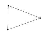
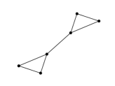
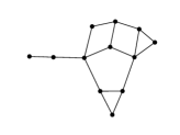
3-Nodes	6-Nodes	12-Nodes

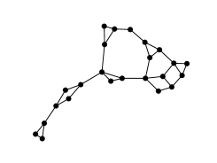
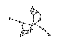
24-Nodes	48-Nodes

Figure 1: Topologies of the different graphs connecting buildings in the microgrids

3.2 Resolution algorithms

We reconsider the two decomposition algorithms introduced in §2.3 and apply them to each problem described in Figure 1. We will term Dual Approximate Dynamic Programming (DADP) the price decomposition algorithm described in §2.3.1 and Primal Approximate Dynamic Programming (PADP) the resource decomposition algorithm described in §2.3.2. We compare DADP and PADP with the well-known Stochastic Dual Dynamic Programming (SDDP) algorithm (see girardeau2014convergence and references inside) applied to the global problem.

3.2.1 Gradient-like algorithms

It is common knowledge that the usual gradient descent algorithm may be slow to converge. To overcome this issue, we use a quasi-Newton algorithm to approximate numerically the Hessian of the two global value functions $p\mapsto\underline{V}[p](x_{0}^{1},\cdots,x_{0}^{N_{\mathcal{V}}})$ in (12) and $r\mapsto\overline{V}[r](x_{0}^{1},\cdots,x_{0}^{N_{\mathcal{V}}})$ in (16). More precisely, the quasi-Newton algorithm is performed using Ipopt 3.12 compiled with the MUMPS linear solver (see (wachter2006implementation, )). The algorithm stops either when a stopping criterion is fulfilled or when no descent direction is found.

3.2.2 SDDP on the global problem

In order to have at disposal a reference solution for the global problem (8), we solve it using the Stochastic Dual Dynamic Programming (SDDP) method. But the SDDP algorithm is not implementable in a straightforward manner. Indeed, the cardinality of the global noise support becomes huge with the number of nodes $N_{\mathcal{V}}$ (see Table 1), so that the exact computation of expectations, as required at each time step during the backward pass of the SDDP algorithm (see shapiro10 ), becomes untractable. To overcome this issue, we resample the probability distribution of the global noise $(\boldsymbol{W}_{t}^{1},\cdots,\boldsymbol{W}_{t}^{N_{\mathcal{V}}})$ for each time $t$ to deal with a noise support of reasonable size. To do so, we use the $k$-means clustering method, as described in rujeerapaiboon2018scenario . By using the Jensen inequality w.r.t. the noises, we know that the optimal quantization of a finite distribution yields a new optimization problem whose optimal value is a lower bound for the optimal value of the original problem, provided that the local problems are convex w.r.t. the noises (see lohndorfmodeling for details). Then, the exact lower bound given by SDDP with resampling remains a lower bound for the exact lower bound given by SDDP without resampling, which istself is a lower bound for the original problem by construction. In the numerical application, we fix the resampling size to $100$. We denote by $\{\underline{V}^{\mathrm{sddp}}_{t}\}_{t=0,\cdots,T}$ the value functions returned by the SDDP algorithm. Notice that, whereas the SDDP algorithm suffers from the cardinality of the global noise support, the DADP and PADP algorithms do not.

We stop SDDP when the gap between its exact lower bound and a statistical upper bound is lower than 1%. That corresponds to the standard SDDP’s stopping criterion described in shapiro10 , which is reputed to be more consistent than the first stopping criterion introduced in pereira1991multi . SDDP uses a level-one cut selection algorithm (guigues2017dual, ) and keeps only the 100 most relevant cuts. By doing so, we significantly reduce the computation time of SDDP.

3.3 Devising control policies

Each algorithm (DADP, PADP and SDDP) returns a sequence of value functions indexed by time, that allow to build a global control policy. Using these value functions, we define a sequence of global value functions $\{\widehat{V}_{t}\}_{t\in\llbracket 0,T\rrbracket}$ approximating the original value functions:

• $\displaystyle\widehat{V}_{t}=\underline{V}^{\mathrm{sddp}}_{t}$ for SDDP,

• $\displaystyle\widehat{V}_{t}=\sum_{i=1}^{N_{\mathcal{V}}}\underline{V}_{{\mathcal{V}},t}^{i}[p]+\underline{V}_{{\mathcal{E}},t}[p]$ for DADP,

• $\displaystyle\widehat{V}_{t}=\sum_{i=1}^{N_{\mathcal{V}}}\overline{V}_{{\mathcal{V}},t}^{i}[r]+\overline{V}_{{\mathcal{E}},t}[r]$ for PADP.

We use these global value functions to build a global control policy for all time $t\in\llbracket 0,T-1\rrbracket$. For any global state $x_{t}\in\mathbb{X}_{t}$ and global noise $w_{t+1}\in\mathbb{W}_{t+1}$, the control policy is a solution of the following one-step DP problem:

$$\gamma_{t}(x_{t},w_{t+1})\in\mathop{\arg\min}_{u_{t}}\min_{f_{t},q_{t}} \sum_{i=1}^{N_{\mathcal{V}}}L_{t}^{i}(x_{t}^{i},u_{t}^{i},w^{i}_{t+1})\!+\!\sum_{e=1}^{N_{\mathcal{E}}}l_{t}^{e}(q_{t}^{e})\!+\!\widehat{V}_{t+1}\big{(}x_{t+1}\big{)}$$ (23a)

s.t. $$x_{t+1}^{i}={g}_{t}^{i}(x_{t}^{i},u_{t}^{i},w^{i}_{t+1})\;,\enspace\forall i\in\llbracket 1,N_{\mathcal{V}}\rrbracket\;,$$ (23b)

$$\Delta_{t}^{i}(x_{t}^{i},u_{t}^{i},w_{t+1}^{i})=f_{t}^{i}\;,\enspace\forall i\in\llbracket 1,N_{\mathcal{V}}\rrbracket\;,$$ (23c)

$$Aq_{t}+f_{t}=0\;.$$ (23d)

As the strategy induced by (23) is admissible for the global problem (8), the expected value of its associated cost is an upper bound of the optimal value $V_{0}^{\sharp}$ of the original minimization problem (8).

3.4 Numerical results

We first compare the three algorithms depicted in §3.2. We analyze the convergence of them and the CPU time needed for achieving it. We also present the value of the exact bounds obtained by each algorithm. Then we evaluate the quality of the strategies (23) introduced in §3.3 for the three algorithms.

3.4.1 Computation of the Bellman value functions

We solve Problem (8) by SDDP, price decomposition (DADP) and resource decomposition (PADP). Table 2 details the execution time and number of iterations taken before reaching convergence.

Problem	3-Nodes	6-Nodes	12-Nodes	24-Nodes	48-Nodes
$|\mathbb{X}_{t}|$	4	8	16	32	64
SDDP CPU time	1’	3’	10’	79’	453’
SDDP iterations	30	100	180	500	1500
DADP CPU time	6’	14’	29’	41’	128’
DADP iterations	27	34	30	19	29
PADP CPU time	3’	7’	22’	49’	91’
PADP iterations	11	12	20	19	20

Table 2: Convergence results for SDDP, DADP and PADP

For a small-scale problem like 3-Nodes (second column of Table 2), SDDP is faster than DADP and PADP. However, for the 48-Nodes problem (last column of Table 2), DADP and PADP are more than three times faster than SDDP. Figure 2 depicts how much CPU time take the different algorithms with respect to the number of state variables of the district. For this case study, we observe that the CPU time grows almost linearly w.r.t. the number of nodes for DADP and PADP, whereas it grows exponentially for SDDP. Otherwise stated, decomposition methods scale better than SDDP in terms of CPU time for large microgrids instances.

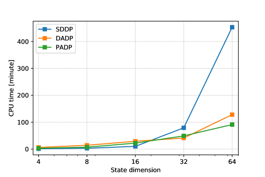
Figure 2: CPU time for the three algorithms as a function of the state dimension

Convergence of the SDDP algorithm.

Figure 3 displays the convergence of SDDP for the 12 nodes problem. The approximate upper bound is estimated every 10 iterations, with 1,000 scenarios. We observe that the gap between the upper and lower bounds is below 1% after 180 iterations. The lower bound remains stable after 250 iterations.

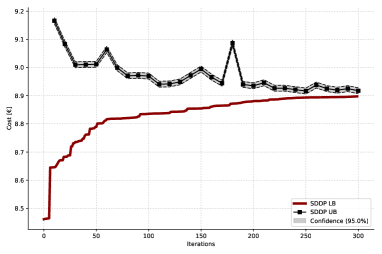
Figure 3: Evolution of SDDP lower and upper bounds for the 12-Nodes problem

DADP and PADP convergence.

We exhibit in Figure 4 the convergence of the DADP’s price process and the PADP’s resource process along iterations for the 12-Nodes problem. We depict the convergence only for the first node, the evolution of price process and resource process in other nodes being similar. On the left side of the figure, we plot the evolution of the 96 different values of the price process $p^{1}=(p^{1}_{0},\cdots,p^{1}_{T-1})$ during the iterations of DADP. We observe that most of the prices start to stabilize after 15 iterations, and do not exhibit sensitive variation after 20 iterations. On the right side of the figure, we plot the evolution of the 96 different values of the resource process $r^{1}=(r_{0}^{1},\cdots,r_{T-1}^{1})$ during the iterations of PADP. We observe that the convergence of resources is quicker than for prices, as the evolution of most resources starts to stabilize after only 10 iterations.

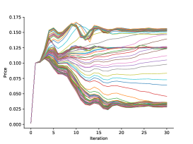
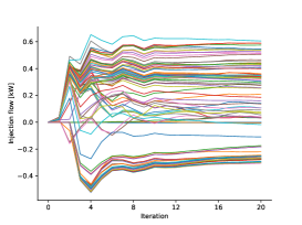
(a)	(b)

Figure 4: Convergence of DADP’s prices (a) and PADP resources (b) for the 12-Nodes problem

Quality of the exact bounds.

We then give the lower and upper bounds obtained by SDDP, DADP, PADP in Table 3. The lower bound of the SDDP algorithm is the value $\underline{V}_{0}^{sddp}(x_{0})$ given by the SDDP method. We recall that SDDP returns a lower bound because it uses a suitable resampling of the global uncertainty distribution instead of the original distribution itself (see the discussion in §3.2.2). DADP and PADP lower and upper bounds are given by Equation (19b) and Equation (21b) respectively. In Table 3, we observe that

• SDDP and DADP lower bounds are close to each other,

• for problems with more than 12 nodes, DADP’s lower bound is up to 2.6% better than SDDP’s lower bound,

• the gap between the upper bound given by PADP and the two lower bounds is rather large.

Problem	3-Nodes	6-Nodes	12-Nodes	24-Nodes	48-Nodes
SDDP LB	225.2	455.9	889.7	1752.8	3310.3
DADP LB	213.7	447.3	896.7	1787.0	3396.4
PADP UB	252.1	528.5	1052.3	2100.7	4016.6

Table 3: Upper and lower bounds given by SDDP, DADP and PADP

To sum up, the important result of this paragraph is that, for optimization problems of large microgrids, DADP is able to compute a slightly better lower bound than SDDP, and compute it much faster than SDDP. A parallel version of DADP would obtain even better performance.

3.4.2 Policy simulation results

We now compare the performances of the different algorithms in simulation. As explained in §3.3, we are able to devise online strategies induced by SDDP, DADP and PADP for the global problem, and to compute by Monte Carlo an approximation of the expected cost of each of these strategies.

The results obtained in simulation are given in Table 4. SDDP, DADP and PADP values are obtained by simulating the corresponding strategies on $5,000$ scenarios. The notation $\pm$ corresponds to the 95% confidence interval. We use the value obtained by the SDDP strategy as a reference, a positive gap meaning that the associated decomposition-based strategy is better than the SDDP strategy. Note that all these values correspond to admissible strategies for the global problem (8), and thus are statistical upper bounds of the optimal cost $V_{0}^{\sharp}$ of Problem (8).

Network	3-Nodes	6-Nodes	12-Nodes	24-Nodes	48-Nodes
SDDP value	226 $\pm$ 0.6	471 $\pm$ 0.8	936 $\pm$ 1.1	1859 $\pm$ 1.6	3550 $\pm$ 2.3
DADP value	228 $\pm$ 0.6	464 $\pm$ 0.8	923 $\pm$ 1.2	1839 $\pm$ 1.6	3490 $\pm$ 2.3
Gap	- 0.8 %	+ 1.5 %	+1.4%	+1.1%	+1.7%
PADP value	229 $\pm$ 0.6	471 $\pm$ 0.8	931 $\pm$ 1.1	1856 $\pm$ 1.6	3508 $\pm$ 2.2
Gap	-1.3%	0.0%	+0.5%	+0.2%	+1.2%

Table 4: Simulation results for strategies induced by SDDP, DADP and PADP

We make the following observations.

• For problems with more than 6 nodes, both the DADP strategy and the PADP strategy beat the SDDP strategy.

• The DADP strategy gives better results than the PADP strategy.

• Comparing with the last line of Table 3, the statistical upper bounds obtained by the three simulation strategies are much closer to SDDP and DADP lower bounds than PADP’s exact upper bound. By assuming that the resource coordination process is deterministic in PADP, we impose constant importation flows for every possible realization of the uncertainties, thus penalizing heavily the PADP algorithm (see also the interpretation of PADP in the case of a decentralized information structure in (bounds2019theory, , §3.3)).

4 Conclusion

In this article, as an application of the companion paper bounds2019theory , we have studied optimization problems where coupling constraints correspond to interaction exchanges on a graph and we have presented a way to decompose them spatially (Sect. 2). We have outlined two decomposition algorithms, the first relying on price decomposition and the second on resource decomposition; they work in a decentralized manner and are fully parallelizable. Then we have used these algorithms on a specific case study (Sect. 3), namely the management of several district microgrids with different prosumers exchanging energy altogether. Numerical results have showed the effectiveness of the approach: the price decomposition algorithm beats the reference SDDP algorithm for large-scale problems with more than 12 nodes, both in terms of exact bound and induced online strategy, and in terms of computation time. On problems with up to 48 nodes (corresponding to 64 state variables), we have observed that their performance scales well as the number of nodes grew: SDDP is affected by the well-known curse of dimensionality, whereas decomposition-based methods are not. Moreover, we have presented in this article a serial version of the decomposition algorithms, and we believe that leveraging their parallel nature could decrease further their computation time.

A natural extension is the following. In this paper, we have only considered deterministic price and resource coordination processes. Using larger search sets for the coordination variables, e.g. considering Markovian coordination processes, would make it possible to improve the performance of the algorithms. However, one would need to analyze how to obtain a good trade-off between accuracy and numerical performance.

References

- (1) Ruszczyński, A.: Decomposition methods in stochastic programming. Mathematical programming 79(1), 333–353 (1997)
- (2) Carpentier, P., Cohen, G.: Décomposition-coordination en optimisation déterministe et stochastique, vol. 81. Springer (2017)
- (3) Shapiro, A., Tekaya, W., da Costa, J.P., Soares, M.P.: Final report for technical cooperation between Georgia Institute of Technology and ONS – Operador Nacional do Sistema Elétrico. Georgia Tech ISyE Report (2012)
- (4) Cohen, G.: Auxiliary Problem Principle and decomposition of optimization problems. Journal of Optimization Theory and Applications 32(3), 277–305 (1980)
- (5) Cohen, G., Culioli, J.C.: Decomposition Coordination Algorithms for Stochastic Optimization. SIAM Journal on Control and Optimization 28(6), 1372–1403 (1990)
- (6) Barty, K., Carpentier, P., Girardeau, P.: Decomposition of large-scale stochastic optimal control problems. RAIRO-Operations Research 44(3), 167–183 (2010)
- (7) Carpentier, P., Chancelier, J.P., De Lara, M., Pacaud, F.: Upper and lower bounds for large scale multistage stochastic optimization problems: Decomposition methods. Preprint (2019)
- (8) Rockafellar, R.T.: Network flows and monotropic optimization. J. Wiley & Sons (1984)
- (9) Bertsekas, D.P.: Extended monotropic programming and duality. Journal of optimization theory and applications 139(2), 209–225 (2008)
- (10) Chatzipanagiotis, N., Dentcheva, D., Zavlanos, M.M.: An augmented Lagrangian method for distributed optimization. Mathematical Programming 152(1-2), 405–434 (2015)
- (11) Pinson, P., Baroche, T., Moret, F., Sousa, T., Sorin, E., You, S.: The emergence of consumer-centric electricity markets. Distribution & Utilization 34(12), 27–31 (2017)
- (12) Pacaud, F.: Decentralized optimization methods for efficient energy management under stochasticity. Thèse de doctorat, Université Paris-Est (2018)
- (13) Schütz, T., Streblow, R., Müller, D.: A comparison of thermal energy storage models for building energy system optimization. Energy and Buildings 93, 23–31 (2015)
- (14) Girardeau, P., Leclere, V., Philpott, A.B.: On the convergence of decomposition methods for multistage stochastic convex programs. Mathematics of Operations Research 40(1), 130–145 (2014)
- (15) Wächter, A., Biegler, L.T.: On the implementation of an interior-point filter line-search algorithm for large-scale nonlinear programming. Mathematical programming 106(1), 25–57 (2006)
- (16) Shapiro, A.: Analysis of Stochastic Dual Dynamic Programming Method. European Journal of Operational Research 209, 63–72 (2011)
- (17) Rujeerapaiboon, N., Schindler, K., Kuhn, D., Wiesemann, W.: Scenario reduction revisited: Fundamental limits and guarantees. Mathematical Programming pp. 1–36 (2018)
- (18) Löhndorf, N., Shapiro, A.: Modeling time-dependent randomness in stochastic dual dynamic programming. European Journal of Operational Research 273(2), 650–671 (2019)
- (19) Pereira, M.V., Pinto, L.M.: Multi-stage stochastic optimization applied to energy planning. Mathematical programming 52(1-3), 359–375 (1991)
- (20) Guigues, V.: Dual dynamic programing with cut selection: Convergence proof and numerical experiments. European Journal of Operational Research 258(1), 47–57 (2017)