NRCPS-HE-01-2020

Maximally Chaotic Dynamical Systems
of Anosov-Kolmogorov

George Savvidy

Institute of Nuclear and Particle Physics

NCSR Demokritos, Ag. Paraskevi, Athens, Greece

Abstract

The maximally chaotic K-systems are dynamical systems which have nonzero Kolmogorov entropy. On the other hand, the hyperbolic dynamical systems that fulfil the Anosov C-condition have exponential instability of phase trajectories, mixing of all orders, countable Lebesgue spectrum and positive Kolmogorov entropy. The C-condition defines a rich class of maximally chaotic systems which span an open set in the space of all dynamical systems. The interest in Anosov-Kolmogorov C-K systems is associated with the attempts to understand the relaxation phenomena, the foundation of the statistical mechanics, the appearance of turbulence in fluid dynamics, the non-linear dynamics of the Yang-Mills field as well as the dynamical properties of gravitating N-body systems and the Black hole thermodynamics. In this respect of special interest are C-K systems that are defined on Reimannian manifolds of negative sectional curvature and on a high-dimensional tori. Here we shall review the classical- and quantum-mechanical properties of maximally chaotic dynamical systems, the application of the C-K theory to the investigation of the Yang-Mills dynamics and gravitational systems as well as their application in the Monte Carlo method.

1 Introduction

It seems natural to define the maximally chaotic dynamical systems as systems that have nonzero Kolmogorov entropy [1, 2]. A large class of maximally chaotic dynamical systems was constructed by Anosov [3]. These are the systems that fulfil the C-condition. The Anosov C-condition leads to the exponential instability of phase trajectories, to the mixing of all orders, countable Lebesgue spectrum and positive Kolmogorov entropy. The uniqueness of the Anosov C-condition lies in the fact that it allows to define a rich class of maximally chaotic systems that span an open set in the space of all dynamical systems. The examples of maximally chaotic systems were discovered and discussed in the earlier investigations by Artin, Hadamard, Hedlund, Hopf, Birkhoff and others [9, 13, 14, 16, 15, 18, 19, 20, 21, 22, 23, 24, 25, 26] as well as in more recent investigations [51, 52, 53, 54, 55, 56, 57, 58, 59, 60, 61, 62, 63, 12]. Here we shall introduce and discuss the classical- and quantum-mechanical properties of maximally chaotic dynamical systems, the application of the C-K theory to the investigation of the gauge and gravitational systems as well as their application in the Monte Carlo method.

In recent years the alternative concept of maximally chaotic systems was developed in series of publications [40, 41, 42, 43, 43, 44, 45, 46] and references therein. It is based on the analysis of the quantum-mechanical properties of the black holes physics and on the investigation of the so called out-of-time correlation functions. In general the two- and many-point thermodynamical correlation functions decay exponentially. It was observed that the thermodynamics of black holes exhibits extraordinary property of fast relaxation and of the exponential growth of the out-of-time correlation functions. Such chaotic behaviour has come to be referred to as ”scrambling,” and it has been conjectured that black holes are the fastest scramblers in nature. The influence of chaos on the time dependent commutator of two observables can develop no faster than exponentially with the exponent ${2\pi\over\beta}t=2\pi Tt$, which is growing linearly in temperature $1/\beta=T$ and time $t$. This maximal linear growth is saturated in gravitational and dual to the gravity systems [40, 41, 42]. One of our aims is to calculate out-of-time correlation functions in the case of C-K systems and to check if their quantum-mechanical correlation functions grow exponentially and if the exponent grows linearly with temperature. That can help to understand better the concept of maximally chaotic dynamical systems and their role in thermalisation phenomena.

This review is organised as follows. In the second section we shall discuss the classification of the dynamical systems (DS) by the increase of their statistical-chaotic properties [25, 26]. These are ergodic, mixing, n-fold mixing and finally the K-systems, which have mixing of all orders and nonzero Kolmogorov entropy. This consideration defines the hierarchy of DS by their increasing chaotic/stochastic properties, with maximally chaotic K-systems on the ”top”. The question is: Do the maximally chaotic systems exist? The hyperbolic C-systems introduced by Anosov represent a large class of K-systems defined on the Riemannian manifolds of negative sectional curvature and on high-dimensional tori.

We shall consider the general properties of the C-systems in the third section. From the C-condition it follows that C-systems have very strong instability of their trajectories and, in fact, the instability is as strong as it can be in principle [3, 19]. The distance between infinitesimally close trajectories increases exponentially and on a closed phase space of the dynamical system this leads to the uniform distribution of almost all trajectories over the whole phase space. The dynamical systems which fulfil the C-condition have very extended and rich ergodic properties [3]. The C-condition, in most of the cases, is a sufficient condition for the dynamical system to be a K-system as well. In this sense the C-systems provide extended and rich list of concrete examples of K-systems. The other important property of the C-systems is that in ”between” the uniformly distributed trajectories there is a countable set of periodic trajectories. The set of points on the periodic trajectories is everywhere dense in the phase space. The periodic trajectories and uniformly distributed trajectories are filling out the phase space of a C-system in a way very similar to the rational and irrational numbers on the real line.

The hyperbolic geodesic flow on Riemannian manifolds of negative sectional curvature will be considered in fourth section [3, 14, 16, 15, 18]. It was proven by Anosov that the geodesic flow on closed Riemannian manifold of negative sectional curvature fulfils the C-condition and therefore defines a large class of maximally chaotic systems with nonzero Kolmogorov entropy. This result provides a powerful tool for the investigation of the Hamiltonian systems. If the time evolution of a classical physical system under investigation can be reformulated as the geodesic flow on the Riemannian manifold of negative sectional curvature, then all ergodic/chaotic properties of the C-K systems can be ascribed to that physical system. The C-K systems have a tendency to approach the equilibrium state with exponential rate which is proportional to the entropy. The larger the entropy is, the faster a physical system tends to its equilibrium.

In the fifth section we shall consider the classical and quantum dynamics of the Yang-Mills fields [27, 28, 29, 30, 31, 32, 36, 37, 38, 40, 41, 43, 44, 45, 46]. In the case of space homogeneous gauge fields the Yang-Mills equations become equivalent to the classical-mechanical system, the Yang-Mills classical mechanics (YMCM), which has finite degrees of freedom. Using energy and momentum conservation integrals the system can be reduced to a system of lower dimension, and the fundamental question is if the residual system has additional hidden conserved integrals. The evolution of the YMCM can be formulated as the geodesic flow on a Riemannian manifold with the Maupertuis’s metric. The investigation of the sectional curvature demonstrates that it is negative on the equipotential surface and generates exponential instability of the trajectories. The numerical integration also confirms this conclusion. The natural question which arrises here is to what extent the classical chaos influences the quantum-mechanical properties of the gauge fields. The corresponding quantum-mechanical system represents and defines a quantum-mechanical matrix system [31, 32]. We shall discuss its spectral properties and the traces of the classical chaos in its quantum-mechanical regime.

The interesting application of the Anosov C-systems theory was found in the investigation of the relaxation phenomena in stellar systems like globular clusters and galaxies [47, 49]. Here again one can use the Maupertuis’s metric in order to reformulate the evolution of N-body system in Newtonian gravity as a geodesic flow on a Riemannian manifold. Investigation of the sectional curvature allows to estimate the average value of the exponential divergency of the phase trajectories and the relaxation time toward the Maxwellian distribution of the stars velocities in elliptic galaxies and globular clusters [47]. This time is by few orders of magnitude shorter than the Chandrasekchar binary relaxation time [48, 50]. The difference is rooted in the fact that in this approach one can take into account the long-range interaction of stars through their collective contribution into the sectional curvature which defines the relaxation time.

Of special interest are continuous C-systems which are defined on the two-dimensional surfaces embedded into the hyperbolic Lobachevsky plane of constant negative curvature [10]. An example of such system has been defined in a brilliant article published in 1924 by the mathematician Emil Artin [9]. The dynamical system is defined on the fundamental region of the Lobachevsky plane that is obtained by the identification of points congruent with respect to the modular group $SL(2,Z)$, a discrete subgroup of the Lobachevsky plane isometries $SL(2,R)$ [5, 6, 7, 8]. The fundamental region in this case is a hyperbolic triangle, a non-compact region of a finite area. The geodesic trajectories are bounded to propagate on the fundamental hyperbolic triangle and are exponentially unstable. In classical regime the exponential divergency of the geodesic trajectories resulted into the universal exponential decay of the classical correlation functions [10, 86, 87, 88, 89, 90]. The Artin symbolic dynamics, the differential geometry and group-theoretical methods of Gelfand and Fomin [85] are used to investigate the exponential decay rate of the classical correlation functions in the seventh section [10].

There is a great interest in considering quantisation of the hyperbolic dynamical systems and investigation of their quantum-mechanical properties. This subject is very closely related to the investigation of quantum mechanics of classically chaotic systems in gravity [40, 42, 41]. In the eighth section we shall study the behaviour of the correlation functions of the Artin hyperbolic dynamical system in the quantum-mechanical regime. In order to investigate the behaviour of the correlation functions in the quantum-mechanical regime it is necessary to know the spectrum of the system and the corresponding wave functions. In the case of the modular group the energy spectrum has continuous part, which is originating from the asymptotically free motion inside an infinitely long channel extended in the vertical direction of the fundamental region, as well as infinitely many discrete energy states corresponding to a bounded motion at the ”bottom” of the fundamental triangle [91, 92, 93, 94, 95, 97, 98, 99, 104, 100, 101]. The spectral problem has deep number-theoretical origin and was partially solved in a series of pioneering articles [91, 92, 93, 94]. It was solved partially because the discrete spectrum and the corresponding wave functions are not known analytically. The general properties of the discrete spectrum have been derived by using Selberg trace formula [93, 94, 95, 97, 98, 99]. Numerical calculations of the discrete energy levels were performed for many energy states [104, 100, 101]. In the eighth section we shall describe the quantisation of the Artin system and shall review the derivation of the Maass wave functions describing the continuous spectrum.

Having in hand the explicit expression of the wave functions one can analyse the quantum-mechanical behaviour of the correlation functions in order to investigate the traces of the classical chaos in quantum-mechanical regime [11]. In the ninth section we shall consider the correlation functions of the Louiville-like operators and shall demonstrate that all two- and four-point correlation functions decay exponentially with time, with the exponents which depend on temperature. Alternatively to the exponential decay of the correlation functions the square of the commutator of the Louiville-like operators separated in time grows exponentially [11]. This growth is reminiscent to the local exponential divergency of trajectories of the Artin system when it was considered in the classical regime. The exponential growth of the commutator does not saturate the condition of maximal growth which was conjectured to be linear in temperature in the case of the gravitational systems and BH thermodynamics [40, 41, 42]. In calculation of the quantum-mechanical correlation functions a perturbative expansion is used in which the high-mode Bessel’s functions are considered as perturbations. It has been found that calculations are stable with respect to these perturbations and do not influence the final results. The reason is that in the integration region of the matrix elements the high-mode Bessel’s functions are exponentially small.

In the tenth section we shall demonstrate that the Riemann zeta function zeros [4] define the position and the widths of the resonances of the quantised Artin hyperbolic system [12]. A possible relation of the zeta function zeros and quantum-mechanical spectrum was discussed in the passed, David Hilbert seems to have proposed the idea of finding an eigenvalue problem whose spectrum contains the zeros of $\zeta(s)$ [63]. The quantum-mechanical resonances have more complicated pole structure compared to that in the case of a pure discrete spectrum and can be adequately described in terms of the scattering S-matrix theory. We shall use the S-matrix approach to analyse the scattering phenomenon in quantised Artin system. As it was discussed above, the Artin dynamical system is defined on the fundamental region of the modular group on the Lobachevsky plane. It has a finite area and an infinite extension in the vertical direction that correspond to a cusp. In quantum-mechanical regime the system can be associated with the narrow infinitely long waveguide stretched out to infinity along the vertical axis and a cavity resonator attached to it at the bottom. That suggests a physical interpretation of the Maass automorphic wave function in the form of an incoming plane wave of a given energy entering the resonator and bouncing back to infinity. As the energy of the incoming wave comes close to the eigenmodes of the cavity a pronounced resonance behaviour shows up in the scattering amplitude. The condition of the absence of incoming waves allows to find the position of the pole singularities [12]. The poles of the S-martrix are located in the energy complex plane and are expressed in terms of zeros $u_{n}$ of the Riemann zeta function $\zeta(\frac{1}{2}-iu_{n})=0,~{}~{}~{}~{}n=1,2,....$ as

$$E=E_{n}-i{\Gamma_{n}\over 2}=({u^{2}_{n}\over 4}+{3\over 16})-i{u_{n}\over 2},$$

where $E_{n}$ is the energy and $\Gamma_{n}$ is the width of the n’th resonance. The conclusion is that the energy spectrum is quasi-discrete, consisting of smeared levels of width $\Gamma_{n}$ [12].

In the last, eleventh, section we shall turn our attention to the investigation of the second class of the C-K systems that is defined on high-dimensional tori [3]. In order that the automorphisms of a torus fulfils the C-condition it is necessary and sufficient that the evolution operator $T$ has no eigenvalues on a unit circle and the determinant is equal to one. Therefore $T$ is an automorphism of the torus onto itself. All trajectories with rational coordinates, and only they, are periodic trajectories of the automorphisms of a torus. The entropy of the C-system on a torus is equal to the logarithmic sum of all eigenvalues that lie outside of the unit circle [3, 55, 56, 58, 59, 60, 61]: $h(T)=\sum_{|\lambda_{\beta}|>1}\ln|\lambda_{\beta}|.$ It was suggested in 1986 [68] to use the C-K systems defined on a torus to generate high quality pseudorandom numbers for Monte-Carlo method [64, 65, 66, 67, 68, 80, 81]. Usually pseudorandom numbers are generated by deterministic recursive rules [68, 64, 65, 66, 67]. Such rules produce pseudorandom numbers, and it is a great challenge to design pseudorandom number generators that produce high quality sequences. Although numerous RNGs introduced in the last decades fulfil most of the requirements and are frequently used in simulations, each of them has some weak properties that influence the results [79] and are less suitable for demanding MC simulations [75]. The high entropy MIXMAX generator suggested in [68, 69, 70, 71] was implemented into the Geant4/CLHEP and ROOT scientific toolkits at CERN [73, 75, 76, 74].

The Appendix $A$ contains the extended discussion of the C-condition, the definition of the exponentially expanding and contracting foliations.

In [3] Anosov demonstrated how any C-cascade on a torus can be embedded into a certain C-flow. The Appendix $B$ describes the Anosov construction that allows to embed a discrete time evolution on a torus into an evolution that is continuous in time. The embedding was defined by a specific identification of the phase space coordinates and by construction of the corresponding C-flow on a smooth Riemannian manifold of higher dimension. In Anosov construction the C-flow was not a geodesic flow. Here we were interested in analysing the geodesic flow on the same Riemannian manifold. We present the calculation of the corresponding sectional curvatures and demonstrate that the geodesic flow has different dynamics and hyperbolic components.

The Appendix $C$ describes the details of the computer implementation of the torus automorphisms, the computation of the periods of generated random sequences for Monte Carlo simulations. In a typical computer implementation of the torus automorphisms the initial vector will have rational components. If the denominator is taken to be a prime number, then the recursion is realised on extended Galois field $GF[p^{N}]$ and allows to find the period of the trajectories in terms of $p$ and the properties of the characteristic polynomial of the evolution operator.

The Appendix $D$ presents the derivation of the explicit formulas for the Kolmogorov entropy in case of torus automorphisms. The Appendix $E$ presents the discussion of the properties of the periodic trajectories and their density distribution as a function of Kolmogorov entropy.

2 Hierarchy of Dynamical Systems and Kolmogorov Entropy

In ergodic theory the dynamical systems (DS) are classified by the increase of their statistical-chaotic properties. Ergodic systems are defined as follows [25, 26]. Let $x=(q,p)$ be a point of the phase space $x\in M$ of the Hamiltonian systems. The canonical coordinates are denoted as $q=(q_{1},...,q_{d})$ and $p=(p_{1},...,p_{d})$ are the conjugate momenta. The phase space $M$ is equipped with a positive Liouville measure $d\mu(x)=\rho(q,p)dq_{1}...dq_{d}dp_{1}...dp_{d}$, which is invariant under the Hamiltonian flow. The operator $T^{t}x=x_{t}$ defines the time evolution of the trajectory which was launched from the point $x$ of the phase space. The ergodicity of the DS takes place if [21] :

$$\lim_{t\rightarrow\infty}{1\over t}\int_{0}^{t}dtf(T^{t}x)=\int_{M}f(x)dx,$$ (2.1)

where $f(x)$ is a function/observable defined on the phase space $M$. So time averages equal to space averages in this case. It follows then that

$$\lim_{t\rightarrow\infty}{1\over t}\int_{0}^{t}dtf(T^{t}x)g(x)dx=\int_{M}f(x)dx\int_{M}g(x)dx.$$ (2.2)

Consider the function $f=\chi_{A}$ on the phase space which is equal to one on a set $A\subset M$ and to zero outside, similar function $g=\chi_{B}$ for a set $B\subset M$, then

$$\lim_{t\rightarrow\infty}{1\over t}~{}\int_{0}^{t}dt~{}\mu[T^{t}A\cap B]=\mu[A]\mu[B],$$ (2.3)

that is a part of the set $A$ which falls into the set $B$ is in average proportional to their measures. The systems with stronger chaotic properties has been defined by Gibbs [20, 25]. The mixing takes place if for any two sets

$$\lim_{t\rightarrow\infty}\mu[T^{t}A\cap B]=\mu[A]\mu[B],$$ (2.4)

that is a part of set $A$ which falls into the set $B$ is proportional to their measures. Alternatively

$$\lim_{t\rightarrow\infty}\int f(T^{t}x)g(x)dx=\int_{M}f(x)dx\int_{M}g(x)dx,$$ (2.5)

which means that the two-point correlation function tends to zero:

$${\cal D}_{t}(f,g)=\lim_{t\rightarrow\infty}\langle f(T^{t}x)g(x)\rangle-\langle f(x)\rangle\langle g(x)\rangle=0,$$ (2.6)

and is known in physical language as the factorisation property of the two-point correlation functions. The n-fold mixing takes place if for any $n$ sets

$$\lim_{t_{n},...,t_{1}\rightarrow\infty}\mu[T^{t_{n}}A_{n}\cap....T^{t_{2}}A_{2}\cap T^{t_{1}}A_{1}\cap B]=\mu[A_{n}]...\mu[A_{2}]\mu[A_{1}]\mu[B]$$ (2.7)

or alternatively

$${\cal D}_{t}(f_{n},...,f_{1},g)=\lim_{t_{n},...,t_{1}\rightarrow\infty}\langle f_{n}(T^{t_{n}}x).....f_{1}(T^{t_{1}}x)g(x)\rangle-\langle f_{n}(x)\rangle.....\langle f_{1}(x)\rangle\langle g(x)\rangle=0.$$ (2.8)

A class of dynamical systems which have even stronger chaotic properties was introduced by Kolmogorov in [1, 2]. These are the DS which have a non-zero entropy, so called quasi-regular DS, or simply K-systems. In order to define the Kolmogorov entropy let us consider a discrete time evolution operator $T^{n}x=x_{n},~{}n=0,1,2,..$. Let $\alpha=\{A_{i}\}_{i\in I}$ ( $I$ is finite or countable) be a measurable partition of the phase space $M$ into the nonintersecting subsets $A_{i}$ which cover the whole phase space $M$, that is

$$\mu(M\setminus\bigcup_{i\in I}A_{i})=0,~{}~{}~{}~{}\mu(A_{i}\bigcap A_{j})=0,i\neq j~{},$$ (2.9)

and define the entropy of the partition $\alpha$ as

$$h(\alpha)=-\sum_{i\in I}\mu(A_{i})\ln\mu(A_{i}).$$ (2.10)

If two partitions $\alpha_{1}$ and $\alpha_{2}$ differ by a set of measure zero, then their entropies are equal. The refinement partition $\alpha$

$$\alpha=\alpha_{1}\vee\alpha_{2}\vee...\vee\alpha_{k}$$ (2.11)

of the collection of partitions $\alpha_{1},...,\alpha_{k}$ is defined as the intersection of all their composing sets $A_{i}$:

$$\alpha=\big{\{}\bigcap_{i\in I}A_{i}~{}|~{}A_{i}\in\alpha_{i}~{}for~{}all~{}i\big{\}}.$$ (2.12)

The entropy of the partition $\alpha$ with respect to the automorphisms T is defined as a limit [1, 2, 23, 51, 53, 54]:

$$h(\alpha,T)=\lim_{n\rightarrow\infty}{h(\alpha\vee T\alpha\vee...\vee T^{n-1}\alpha)\over n},~{}~{}~{}~{}n=1,2,...$$ (2.13)

This number is equal to the entropy of the refinement $\beta=\alpha\vee T\alpha\vee...\vee T^{n-1}\alpha$ which was generated during the iteration of the partition $\alpha$ by the automorphism $T$. Finally the entropy of the automorphism $T$ is defined as a supremum:

$$h(T)=\sup_{\{\alpha\}}h(\alpha,T),$$ (2.14)

where the supremum is taken over all partitions $\{\alpha\}$ of $M$. It was proven that the K-systems have mixing of all orders: K-mixing $\supset$ infinite mixing, $\supset$,..n-fold mixing,..$\supset$ mixing $\supset$ ergodicity [1, 2, 23, 51, 53, 54]. The calculation of the entropy for a given dynamical system seems extremely difficult. The theorem proven by Kolmogorov [1, 2] tells that if one finds the so called ”generating partition” $\beta$, then

$$h(T)=h(\beta,T),$$ (2.15)

meaning that the supremum in (2.14) is reached on a generating partition $\beta$. In some cases the construction of the generating partition $\beta$ allows an explicit calculation of the entropy of a given dynamical system [57, 62].

In summary, the above consideration allows to define the hierarchy of DSs with their increasing chaotic properties and with the maximally chaotic K-systems on the ”top”. The question is: Do maximally chaotic systems exist? The hyperbolic C-systems introduced by Anosov [3] represent a large class of K-systems and have additional ergodic properties. We shall consider the C-systems in the next section.

3 Hyperbolic Anosov C-systems

In the fundamental work on geodesic flows on closed Riemannian manifolds $Q^{n}$ of negative curvature [3] Dmitri Anosov pointed out that the basic property of the geodesic flow on such manifolds is the uniform instability of all trajectories, which in physical terms means that in the neighbourhood of every fixed trajectory the trajectories behave similarly to the trajectories in the neighbourhood of a saddle point (see Fig. 1). In other words, the hyperbolic instability of the dynamical system $T^{t}$ which is defined by the equations

$$\dot{x}=f(x)$$ (3.16)

takes place for all solutions $\delta x\equiv\omega$ of the deviation equation

$$\dot{\omega}={\partial f\over\partial x}\bigg{|}_{x(t)=T^{t}x}\omega$$ (3.17)

in the neighbourhood of each phase trajectory $x(t)=T^{t}x$, where $x\in M$. The exponential instability of geodesics on Riemannian manifolds of constant negative curvature has been studied by many authors, beginning with Lobachevsky and Hadamard and especially by Artin [9], Hedlund [14], and Hopf [16]. The concept of exponential instability of a dynamical system trajectories appears to be extremely rich and Anosov suggested to elevate it into a fundamental property of a new class of dynamical systems which he called C-systems. The brilliant idea to consider dynamical systems which have local and homogeneous hyperbolic instability of all trajectories is appealing to the intuition and has very deep physical content. The richness of the concept is expressed by the fact that the C-systems occupy a nonzero volume in the space of dynamical systems [3] and have a non-zero Kolmogorov entropy.

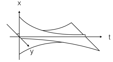
Figure 1: The integral curves in the case of saddle point $\dot{x}=-x,~{}~{}~{}\dot{y}=y$ are exponentially contracting and expanding near the solution $x=y=0$. A similar behaviour takes place in the neighbourhood of almost all trajectories of the C-system [3] as one can get convinced inspecting the solutions (4.29) and (4.30) of the Jacobi variation equation (4.21) with negative sectional curvature (4.28).

Anosov provided an extended list of C-K systems [3]. The important examples of the C-K systems are: i) the geodesic flow on the Riemannian manifolds of variable negative curvature and ii) C-cascades - the iterations of the hyperbolic automorphisms of tori.

In the forthcoming sections we shall consider these maximally chaotic systems in details and the application of the C-K systems theory to the investigation of the Yang-Mills dynamics, the N-body problem in gravity and in the Monte Carlo method. We shall consider the quantum-mechanical properties of the maximally chaotic dynamical systems as well and in particular the DSs which are defined on the closed surfaces of constant negative curvature imbedded into the Lobachevsky hyperbolic plane, the Artin DS [9].

4 The Geodesic Flow on Manifolds of Negative Curvature

Let us consider the stability of the geodesic flow on a Riemannian manifold $Q$ with local with coordinates $q^{\alpha}\in Q$ where $\alpha=1,2,....,3N$. The functions $q^{\alpha}(s)\in Q$ define a one-parameter integral curve $\gamma(s)$ on a Riemannian manifold $Q$ and the corresponding velocity vector

$$u^{\alpha}={dq^{\alpha}\over ds},~{}~{}~{}~{}~{}~{}\alpha=1,2,....,3N~{}.$$ (4.18)

The proper time parameter $s$ along the $\gamma(s)$ is equal to the length, while the Riemannian metric on $Q$ is defined as

$$ds^{2}=g_{\alpha\beta}dq^{\alpha}dq^{\beta},$$

and therefore

$$g_{\alpha\beta}u^{\alpha}u^{\beta}=1.$$ (4.19)

A one-parameter family of deformations assumed to form a congruence of world lines $q^{\alpha}(s)\rightarrow q^{\alpha}(s,\upsilon).$ In order to characterise the infinitesimal deformation of the curve $\gamma(s)$ it is convenient to define a separation vector $\delta q^{\alpha}={\partial q^{\alpha}\over\partial\upsilon}d\upsilon,$ where $\delta q^{\alpha}$ is a separation of points having equal distance from some arbitrary initial points along two neighbouring curves.

The resulting phase space manifold $(q(s),u(s))\in M$ has a bundle structure with the base $q\in Q$ and the spheres $S^{3N-1}$ of unit tangent vectors $u^{\alpha}$ (4.19) as fibers. The integral curve $\gamma(s)$ fulfils the geodesic equation

$${d^{2}q^{\alpha}\over ds^{2}}+\Gamma^{\alpha}_{\beta\gamma}{dq^{\beta}\over ds}{dq^{\gamma}\over ds}=0$$ (4.20)

and the relative acceleration depends only on the Riemann curvature:

$${D^{2}\delta q^{\alpha}\over ds^{2}}=-R^{\alpha}_{\beta\gamma\sigma}u^{\beta}\delta q^{\gamma}u^{\sigma}.$$ (4.21)

The above form of the Jacobi equation is difficult to analyse, first of all because it is written in terms of covariant derivatives $Du^{\alpha}=du^{\alpha}+\Gamma^{\alpha}_{\beta\gamma}u^{\beta}dq^{\gamma}$. And secondly because it is written in terms of separation of points on trajectories instead of distance between trajectories. Following Anosov it is convenient to represent the Jacobi equation in terms of simple derivatives. The norm of the deviation $\delta q$ has the form $|\delta q|^{2}\equiv g_{\alpha\beta}\delta q^{\alpha}\delta q^{\beta}$ and its second derivative is

$${d^{2}\over ds^{2}}|\delta q|^{2} = 2g_{\alpha\beta}\delta q^{\alpha}{D^{2}\delta q^{\beta}\over ds^{2}}+2g_{\alpha\beta}{D\delta q^{\alpha}\over ds}{D\delta q^{\beta}\over ds}.$$ (4.22)

Using (4.21) we shall get the Anosov form of the Jacobi equation

$${d^{2}\over ds^{2}}|\delta q|^{2} = -2R_{\alpha\beta\gamma\lambda}\delta q^{\alpha}u^{\beta}\delta q^{\gamma}u^{\lambda}+2|{D\delta q\over ds}|^{2}=-2K(q,u,\delta q)~{}|u\wedge\delta q|^{2}+2|\delta u|^{2}~{}~{}~{}~{}~{}~{}~{}$$ (4.23)

where $K(q,u,\delta q)$ is the sectional curvature in the two-dimensional directions defined by the velocity vector $u^{\alpha}$ and the deviation vector $\delta q^{\beta}:$

$$K(q,u,\delta q)={R_{\alpha\beta\gamma\sigma}\delta q^{\alpha}u^{\beta}\delta q^{\gamma}u^{\sigma}\over|u\wedge\delta q|^{2}}.$$ (4.24)

One can decompose the deviation vector $\delta q$ into longitudinal and transversal components $\delta q^{\alpha}=\delta q^{\alpha}_{\perp}+\delta q^{\alpha}_{\parallel},$ where $\delta q_{\parallel}$ describes a translation along the geodesic trajectories and has no physical interest, the transversal component $\delta q_{\perp}$ describes a physically relevant distance between original and infinitesimally close trajectories $|u\delta q_{\perp}|=0$. Such decomposition allows to rederive the Jacobi equation only in terms of transversal deviation:

$${d^{2}\over ds^{2}}|\delta q_{\perp}|^{2} = -2K(q,u,\delta q_{\perp})~{}|\delta q_{\perp}|^{2}+2|\delta u_{\perp}|^{2}.$$ (4.25)

Because the last term is positive definite the following inequality takes place for relative acceleration:

$${d^{2}\over ds^{2}}|\delta q_{\perp}|^{2}\geq-2K(q,u,\delta q_{\perp})~{}|\delta q_{\perp}|^{2}.$$ (4.26)

If the sectional curvature is negative and uniformly bound from above by a constant $\kappa$:

$$K(q,u,\delta q_{\perp})\leq-\kappa<0,~{}~{}~{}\text{where}~{}~{}~{}~{}~{}\kappa=\min_{(q,u,\delta q_{\perp})}|K(q,u,\delta q_{\perp})|$$ (4.27)

then

$${d^{2}\over ds^{2}}|\delta q_{\perp}|^{2}\geq 2\kappa~{}|\delta q_{\perp}|^{2}.$$ (4.28)

The phase space of solutions of the second-order differential equation is divided into two separate sets $X_{q}$ and $Y_{q}$ . The set $Y_{q}$ consists of the solutions with positive first derivative

$${d\over ds}|\delta q_{\perp}(0)|^{2}>0$$

and exponentially grows with $s\rightarrow+\infty$

$$|\delta q_{\perp}(s)|\geq{1\over 2}|\delta q_{\perp}(0)|e^{\sqrt{2\kappa}s},$$ (4.29)

while the set $X_{q}$ consists of the solutions with negative first derivative

$${d\over ds}|\delta q_{\perp}(0)|^{2}<0$$

and decay exponentially with $s\rightarrow+\infty$

$$|\delta q_{\perp}(s)|\leq{1\over 2}|\delta q_{\perp}(0)|e^{-\sqrt{2\kappa}s}.$$ (4.30)

This proves that the geodesic flow on closed Riemannian manifold of negative curvature fulfils the C-conditions, is therefore maximally chaotic and tends to equilibrium with exponential rate. We shall define a relaxation time as

$$\tau=1/\sqrt{2\kappa}~{},$$ (4.31)

which is inversely proportional to the Kolmogorov entropy.

5 The Yang-Mills Classical and Quantum Mechanics

For space-homogeneous gauge fields $\partial_{i}A^{a}_{k}=0$, $i,k=1,2,3$ the Yang-Mills system reduces to a classical mechanical system with the Hamiltonian of the form [27, 28, 30, 31, 32]

$$H=\sum_{i}{1\over 2}Tr\dot{A}_{i}\dot{A}_{i}+{g^{2}\over 4}\sum_{i,j}Tr[A_{i},A_{j}]^{2},$$ (5.32)

where the gauge field $A^{a}_{i}(t)$ depends only on time, $i=1,2,3$, the index $a=1,...,N^{2}-1$ for $SU(N)$ group and in the Hamiltonian gauge $A_{0}=0$ the Gaussian constraint has the form

$${\cal G}=[\dot{A}_{i},A_{i}]=0.$$ (5.33)

It is natural to call this system the Yang-Mills Classical Mechanics (YMCM). It is a mechanical system with $3\cdot(N^{2}-1)$ degrees of freedom. It is important to investigate classical equations of motion of this class of non-Abelian gauge fields, the properties of the separate solutions and of the system as a whole. In particular its integrability versus chaotic properties of the system. The YMCM has a number of conserved integrals: the space and isospin angular momenta

$$m_{i}=\epsilon_{ijk}A^{a}_{j}\dot{A}^{a}_{k},~{}~{}~{}n^{a}=f^{abc}A^{a}_{i}\dot{A}^{a}_{i},~{}~{}~{}i=1,2,3~{}~{}~{}~{}a=1,...,N^{2}-1$$ (5.34)

in total $3+(N^{2}-1)$ integrals, plus the energy integral (5.32) (the $n^{a}=0$ is the constraint (5.33) ). The question is if there exist additional conservation integrals. If the number of integrals coincides with the number of degrees of freedom, then the system is exactly integrable and its trajectories lie on high-dimensional tori, if there are less integrals, then the trajectories lie on a manifold of a larger dimension, and if there is no conserved integrals at all, then the trajectories will cover the whole phase space.

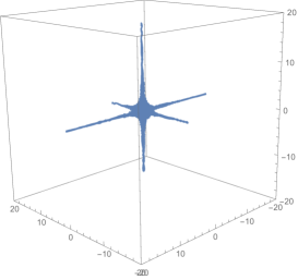
Figure 2: A single trajectory of the YMCM system integrated over a large time interval. The trajectory scatters on the equipotential surface $x^{2}_{1}x^{2}_{2}+x^{2}_{2}x^{2}_{3}+x^{2}_{3}x^{2}_{1}=1$, densely filling the interior region and making visible the six channels of the equipotential surface on which a trajectory scatters.

Let us consider in details the case of the $SU(2)$ gauge group by introducing the angular variables which allow to separate the angular motion from the oscillations by using the substitution

$$A=O_{1}EO^{T}_{2},$$ (5.35)

where $E=(x(t),y(t),z(t))$ is a diagonal matrix and $O_{1},O_{2}$ are orthogonal matrices in Euler angular parametrisation. In this variables the Hamiltonian (5.33) will take the form

$$H_{FS}={1\over 2}(\dot{x}^{2}+\dot{y}^{2}+\dot{z}^{2})+{g^{2}\over 2}(x^{2}y^{2}+y^{2}z^{2}+z^{2}x^{2})+T_{YM},$$ (5.36)

where $T_{YM}$ is the rotational kinetic energy of the the Yang-Mills ”top” spinning in space and isospace. The question is whether the YMCM system (5.36) is an integrable system or not [28, 30, 31]. The general behaviour of the colour amplitudes $(x(t),y(t),z(t))$ in time is characterised by rapid oscillations, decrease in some colour amplitudes and growth in others, colour ”beats” [28] Fig.2. The strong instability of the trajectories with respect to small variations of the initial conditions in the phase space led to the conclusion that the system is stochastic and non-integrable. The search of the conserved integrals of the form $F(p_{x},p_{y},p_{z},x,y,z)$ fulfilling the equation $\{F,H_{FS}\}=0$ also confirms their absence, except the Hamiltonian itself. The evolution of the YMCM can be formulated as the geodesic flow on a Riemannian manifold with the Maupertuis’s metric (see the details in the next section). The investigation of the sectional curvature demonstrates that it is negative on the equipotential surface and generates exponential instability of the trajectories Fig.2. The solutions of an YMCM system in an arbitrary coordinate system (after Lorentz boost) are nonlinear plane waves $A^{a}_{\mu}(k\cdot x)$ with a nonzero square of the wave vector $k^{2}=\mu^{2}$ [27] chaotically oscillating in space-time.

The natural question which arrises here is to what extent the classical chaos influences the quantum-mechanical properties of the gauge fields. The significance of the answer to this question consists in the following. In field theory, e.g. in QED, the electromagnetic field is represented in the form of a set of harmonic oscillators whose quantum-mechanical properties (as of an integrable system) are well known, and the interaction between them is taken into account by perturbation theory. Such an approach excellently describes the experimental situation. In QCD the state of things is quite different. The properties of the YMCM as of a C-K-system, cannot be established to any finite order of the perturbation theory. Therefore to understand QCD it seems important to investigate the quantum-mechanical properties of the systems which in the classical limit are maximally chaotic.

The natural question arising now is what quantum-mechanical properties does the system with the Hamiltonian (5.32) possess if in the classical limit $\hbar\rightarrow 0$ it is maximally chaotic. What is the structure of the energy spectrum and of the wave functions of quantised gauge system, if in the classical limit it is maximally chaotic. The Schrödinger equation for the gauge field theory in the $A_{0}=0$ gauge has the following form;

$${1\over 2}\int d^{3}x[-{\delta^{2}\over\delta A^{a}_{i}\delta A^{a}_{i}}+H^{a}_{i}H^{a}_{i}]\Psi[A]=E\Psi[A],$$ (5.37)

where $H^{a}_{i}={1\over 2}\epsilon_{ijk}G^{a}_{jk}(A)$ and the constraint equations are:

$$[\delta^{ab}\partial_{i}+gf^{acb}A^{c}_{i}]{\delta\over\delta A^{b}_{i}}\Psi[A]=0.$$ (5.38)

In case of space-homogeneous fields the equations will reduce to the Yang-Mills quantum-mechanical system (YMQM) with finite degrees of freedom which defines a special class of quantum-mechanical matrix models [31, 32]. At zero angular momentum $\hat{m}_{i}=0$ (5.34) the YMQM Schrödinger equation takes the form (equations (20) and (21) in [32])

$$\Big{\{}-{1\over 2}D^{-1}\partial_{i}D\partial_{i}+{g^{2}\over 2}(x^{2}_{1}x^{2}_{2}+x^{2}_{2}x^{2}_{3}+x^{2}_{3}x^{2}_{1})\Big{\}}\Psi=E\Psi,$$ (5.39)

where $D(x)=|(x^{2}_{1}-x^{2}_{2})(x^{2}_{2}-x^{2}_{3})(x^{2}_{3}-x^{2}_{1})|$. Using the substitution

$$\Psi(x)={1\over\sqrt{D(x)}}~{}\Phi(x)$$ (5.40)

and the fact that the $D(x)$ is a harmonic function $\partial^{2}_{i}D(x)=0$ the equation can be reduced to the form

$$-{1\over 2}\partial^{2}_{i}\Phi+{1\over 2}\sum_{i<j}\Big{(}{1\over(x_{i}-x_{j})^{2}}+{1\over(x_{i}+x_{j})^{2}}+g^{2}x^{2}_{i}x^{2}_{j}\Big{)}\Phi=E\Phi.$$ (5.41)

The analytical investigation of this Schrödinger equation is a challenging problem because the equation cannot be solved by separation of variables as far as all canonical symmetries are already extracted and the residual system possess no continuous symmetries. Nevertheless some important properties of the energy spectrum can be established by calculating the volume of the classical phase space defined by the condition $H(p,q)\leq E$. It follows that classical phase space volume is finite and the energy spectrum of YMQM system is discrete [31, 32]. Typically the classically chaotic systems have no degeneracy of the energy spectrum, the energy levels ”repulse” from each other similar to the distribution of the eigenvalues of the matrices with randomly distributed elements [33, 34, 35].

In the next section we shall consider the $N$-body problem in classical Newtonian gravity analysing the geodesic flow on a Riemannian manifold equipped with the Maupertuis metric.

6 Collective Relaxation of Stellar Systems

The $N$-body problem in Newtonian gravity can be formulated as a geodesic flow on Riemannian manifold with the conformal Maupertuis metric [47]

$$ds^{2}=(E-U)d\rho^{2}=W\sum^{3N}_{\alpha=1}(dq^{\alpha})^{2},~{}~{}~{}~{}~{}U=-G\sum_{a<b}{M_{a}M_{b}\over|\vec{r}_{a}-\vec{r}_{a}|},$$ (6.42)

where $W=E-U$ and $\{q^{\alpha}\}$ are the coordinates of the stars:

$$\{q^{\alpha}\}=\{M^{1/2}_{1}\vec{r}_{1},.....,M^{1/2}_{N}\vec{r}_{N}\},~{}~{}~{}~{}\alpha=1,...,3N.$$ (6.43)

The equation of the geodesics (4.20) on Riemannian manifold with the metric $g_{\alpha\beta}=W\delta_{\alpha\beta}$ in (6.42) has the form

$${d^{2}q^{\alpha}\over ds^{2}}+{1\over 2W}\Big{(}2{\partial W\over\partial q^{\gamma}}{dq^{\gamma}\over ds}{dq^{\alpha}\over ds}-g^{\alpha\gamma}{\partial W\over\partial q^{\gamma}}g_{\beta\delta}{dq^{\beta}\over ds}{dq^{\delta}\over ds}\Big{)}=0$$ (6.44)

and coincides with the classical N-body equations when the proper time interval $ds$ is replaced by the time interval $dt$ of the form $ds=\sqrt{2}Wdt$. The Riemann curvature in (4.21) for the Maupertuis metric has the form

$$R_{\alpha\beta\gamma\delta} = {1\over 2W}[W_{\beta\gamma}g_{\alpha\delta}-W_{\alpha\gamma}g_{\beta\delta}-W_{\beta\delta}g_{\alpha\gamma}+W_{\alpha\delta}g_{\beta\gamma}]-$$ (6.45)

$$- {3\over 4W^{2}}[W_{\beta}W_{\gamma}g_{\alpha\delta}-W_{\alpha}W_{\gamma}g_{\beta\delta}-W_{\beta}W_{\delta}g_{\alpha\gamma}+W_{\alpha}W_{\delta}g_{\beta\gamma}]+$$

$$+ {1\over 4W^{2}}[g_{\beta\gamma}g_{\alpha\delta}-g_{\alpha\gamma}g_{\beta\delta}]W_{\sigma}W^{\sigma},$$

where $W_{\alpha}=\partial W/\partial q^{\alpha}$ , $W_{\alpha\beta}=\partial W/\partial q^{\alpha}\partial q^{\beta}$ and the scalar curvature is

$$R=3N(3N-1)\Big{[}-{\triangle W\over 3NW^{2}}-({1\over 4}-{1\over 2N}){(\nabla W)^{2}\over W^{3}}\Big{]}$$ (6.46)

and $\triangle W=\partial^{2}W/\partial q^{\alpha}\partial q^{\alpha}$,  $\nabla W=(\partial W/\partial q^{\alpha})(\partial W/\partial q^{\alpha})$. Let us now calculate the sectional curvature (4.24):

$$R_{\alpha\beta\gamma\sigma}\delta q^{\alpha}u^{\beta}\delta q^{\gamma}u^{\sigma} = {1\over 2W}[~{}2|uW^{{}^{\prime\prime}}\delta q||u\delta q|-|\delta qW^{{}^{\prime\prime}}\delta q||uu|-|uW^{{}^{\prime\prime}}u||\delta q\delta q|~{}]-$$ (6.47)

$$- {3\over 4W^{2}}[~{}2|uW^{{}^{\prime}}||W^{{}^{\prime}}\delta q||u\delta q|-|\delta qW^{{}^{\prime}}||W^{{}^{\prime}}\delta q||uu|-|uW^{{}^{\prime}}||W^{{}^{\prime}}u||\delta q\delta q|~{}]+$$

$$+ {1\over 4W^{2}}[~{}|u\delta q|^{2}-|uu||\delta q\delta q|~{}]~{}|W^{{}^{\prime}}W^{{}^{\prime}}|.$$

For the normal deviation $q_{\perp}$ we have $|u\delta q_{\perp}|=0$ and taking into account that the velocity is normalised to unity $|uu|=1$ we have

$$R_{\alpha\beta\gamma\sigma}\delta q^{\alpha}_{\perp}u^{\beta}\delta q^{\gamma}_{\perp}u^{\sigma} = \Big{(}~{}{3\over 4W^{2}}|uW^{{}^{\prime}}|^{2}~{}-{1\over 4W^{2}}|W^{{}^{\prime}}W^{{}^{\prime}}|-{1\over 2W}|uW^{{}^{\prime\prime}}u|~{}\Big{)}|\delta q_{\perp}|^{2}$$ (6.48)

$$- {1\over 2W}~{}|\delta q_{\perp}W^{{}^{\prime\prime}}\delta q_{\perp}|+{3\over 4W^{2}}~{}|\delta q_{\perp}W^{{}^{\prime}}|^{2}.$$

Using the average value of the velocity and deviation taken in the form

$$\overline{u^{\alpha}u^{\beta}}={1\over 3N}g^{\alpha\beta}|uu|,~{}~{}~{}~{}~{}\overline{\delta q_{\perp}^{\alpha}\delta q_{\perp}^{\beta}}={1\over 3N}g^{\alpha\beta}|\delta q_{\perp}|^{2}$$ (6.49)

we shall get the following expression:

$$R_{\alpha\beta\gamma\sigma}\delta q^{\alpha}_{\perp}u^{\beta}\delta q^{\gamma}_{\perp}u^{\sigma}=\Big{[}-{1\over 3N}{\triangle W\over W^{2}}-({1\over 4}-{1\over 2N}){(\nabla W)^{2}\over W^{3}}\Big{]}|\delta q_{\perp}|^{2},$$ (6.50)

which is proportional to the scalar curvature (6.46). As the number of stars in galaxies is very large, $N\gg 1$, we shall get that the dominant term in sectional curvature (6.50) is negative:

$$K(q,u,\delta q)={R_{\alpha\beta\gamma\sigma}\delta q^{\alpha}u^{\beta}\delta q^{\gamma}u^{\sigma}\over|\delta q_{\perp}|^{2}}=-{1\over 4}{(\nabla W)^{2}\over W^{3}}<0.$$ (6.51)

Finally the deviation equation (4.26) will take the form

$${d^{2}\over dt^{2}}|\delta q_{\perp}|^{2}\geq{(\nabla W)^{2}\over W}~{}|\delta q_{\perp}|^{2},$$ (6.52)

where we used the relation $ds=\sqrt{2}Wdt$. Thus the relaxation time can be defined as

$$\tau=\sqrt{{W\over(\nabla W)^{2}}}.$$ (6.53)

Now one can estimate the relaxation time of the elliptic galaxies and globular clusters

$$\tau\approx 10^{8}yr\Big{(}{v\over 10km/s}\Big{)}\Big{(}{n\over 1pc^{-3}}\Big{)}^{-2/3}\Big{(}{M\over M_{\odot}}\Big{)}^{-1}$$ (6.54)

by substituting the corresponding mean values for the velocities $v$, densities $n$ and masses of the stars $M$ [47]. This time is by few orders of magnitude shorter than the Chandrasekchar binary relaxation time [48, 49, 50].

7 Correlation Functions of Classical Artin System

Of special interest are continuous C-systems which are defined on closed surfaces on the Lobachevsky plane of constant negative curvature. An example of such system has been defined in a brilliant article published in 1924 by the mathematician Emil Artin. The dynamical system is defined on the fundamental region of the Lobachevsky plane which is obtained by the identification of points congruent with respect to the modular group $SL(2,Z)$, a discrete subgroup of the Lobachevsky plane isometries $SL(2,R)$. The fundamental region in this case is a hyperbolic triangle. The geodesic trajectories are bounded to propagate on the fundamental hyperbolic triangle. The area of the fundamental region is finite and gets a topology of sphere by ”gluing” the opposite edges of the triangle as it is shown on Fig.3 and Fig.8. The Artin symbolic dynamics, the differential geometry and group-theoretical methods of Gelfand and Fomin will be used to investigate the decay rate of the classical and quantum mechanical correlation functions. The following three sections are devoted to the Artin system and are based on the results published in the articles [10, 11, 12].

Let us start with the Poincare model of the Lobachevsky plane, i.e. the upper half of the complex plane: $H$=$\{z\in\mathbb{C}$, $\Im z>0\}$ supplied with the metric (we set $z=x+iy$)

$$ds^{2}=\frac{dx^{2}+dy^{2}}{y^{2}}\,$$ (7.55)

with the Ricci scalar $R=-2$. Isometries of this space are given by $SL(2,\mathbb{R})$ transformations. The $SL(2,\mathbb{R})$ matrix ($a$,$b$,$c$,$d$ are real and $ad-bc=1$ )

$$g=\left(\begin{array}[]{cc}a&b\\ c&d\end{array}\right)$$

acts on a point $z$ by linear fractional substitutions $z\rightarrow\frac{az+b}{cz+d}~{}.$ Note also that $g$ and $-g$ give the same transformation, hence the effective group is $SL(2,\mathbb{R})/\mathbb{Z}_{2}$. We’ll be interested in the space of orbits of a discrete subgroup $\Gamma\subset SL(2,\mathbb{R})$ in $H$. Our main example will be the modular group $\Gamma=SL(2,\mathbb{Z})$. A nice choice of the fundamental region ${\cal F}$ of $SL(2,\mathbb{Z})$ is displayed in Fig.1. The fundamental region ${\cal F}$ of the modular group consisting of those points between the lines $x=-\frac{1}{2}$ and $x=+\frac{1}{2}$ which lie outside the unit circle in Fig.1. The modular triangle ${\cal F}$ has two equal angles $\alpha=\beta=\frac{\pi}{3}$ and the third one is equal to zero, $\gamma=0$, thus $\alpha+\beta+\gamma=2\pi/3<\pi$. The area of the fundamental region is finite and equals to $\frac{\pi}{3}$ and gets a topology of sphere by ”gluing” the opposite edges of the triangle. The invariant area element on the Lobachevsky plane is proportional to the square root of the determinant of the metric (7.55):

$$d\mu(z)={dxdy\over y^{2}}\,.$$ (7.56)

Thus $\text{area}({\cal F})=\int_{-\frac{1}{2}}^{\frac{1}{2}}dx\int_{\sqrt{1-x^{2}}}^{\infty}\frac{dy}{y^{2}}=\frac{\pi}{3}\,.$ Following the Artin construction let us consider the model of the Lobachevsky plane realised in the upper half-plane $y>0$ of the complex plane $z=x+iy\in{\cal C}$ with the Poincaré metric which is given by the line element (7.55).

The Lobachevsky plane is a surface of a constant negative curvature, because its curvature is equal to $R=g^{ik}R_{ik}=-2$ and it is twice the Gaussian curvature $K=-1$. This metric has two well known properties: 1) it is invariant with respect to all linear substitutions which form the group $g\in G$ of isometries of the Lobachevsky plane:

$$w=g\cdot z\equiv\left(\begin{array}[]{cc}a&b\\ c&d\end{array}\right)\cdot z\equiv\frac{az+b}{cz+d},$$ (7.59)

where $a,b,c,d$ are real coefficients of the matrix $g$ and the determinant of $g$ is positive, $ad-bc>0$. The geodesic lines are either semi-circles orthogonal to the real axis or rays perpendicular to the real axis. The equation for the geodesic lines on a curved surface has the form (4.20), where the Christoffer symbols are evaluated for the metric (7.55). The geodesic equations take the form

$$\frac{d^{2}x}{dt^{2}}-\frac{2}{y}\frac{dx}{dt}\frac{dy}{dt}=0\,,~{}~{}~{}~{}~{}\frac{d^{2}y}{dt^{2}}+\frac{1}{y}\left(\frac{dx}{dt}\right)^{2}-\frac{1}{y}\left(\frac{dy}{dt}\right)^{2}=0,$$

and they have two solutions:

$$x(t)-x_{0}=r\tanh\left(t\right),~{}~{}~{}~{}y(t)=\frac{r}{\cosh\left(t\right)}~{}~{}~{} \leftarrow\text{orthogonal semi-circles}~{}$$ (7.60)

$$x(t)=x_{0},~{}~{}~{}~{}~{}~{}~{}~{}~{}~{}~{}~{}~{}~{}~{}~{}~{}~{}~{}~{}~{}~{}y(t)=e^{t}~{}~{}~{} \leftarrow\text{perpendicular rays }~{}.$$

Here $x_{0}\in(-\infty,+\infty),t\in(-\infty,+\infty)$ and $r\in(0,\infty)$. By substituting each of the above solutions into the metric (7.55) one can get convinced that a point on the geodesics curve moves with a unit velocity (4.19)

$${ds\over dt}=1.$$ (7.61)

In order to construct a compact surface ${\cal F}$ on the Lobachevsky plane, one can identify all points in the upper half of the plane which are related to each other by the substitution (7.59) with the integer coefficients and a unit determinant. These transformations form a modular group $SL(2,\mathbb{Z})$. Thus two points $z$ and $w$ are ”identical” if:

$$w=\frac{mz+n}{pz+q},~{}~{}~{}~{}d=\left(\begin{array}[]{cc}m&n\\ p&q\\ \end{array}\right),~{}~{}~{}~{}d\in SL(2,\mathbb{Z})$$ (7.62)

with integers $m$, $n$, $p$, $q$ constrained by the condition $mq-pn=1$. The $SL(2,\mathbb{Z})$ is the discrete subgroup of the isometry transformations $SL(2,\mathbb{R})$ of (7.59). The identification creates a regular tessellation of the Lobachevsky plane by congruent hyperbolic triangles in Fig. 3. The Lobachevsky plane is covered by the infinite-order triangular tiling. One of these triangles can be chosen as a fundamental region. That fundamental region ${\cal F}$ of the above modular group (7.62) is the well known ”modular triangle”, consisting of those points between the lines $x=-\frac{1}{2}$ and $x=+\frac{1}{2}$ which lie outside the unit circle in Fig. 3. The area of the fundamental region is finite and equals to $\frac{\pi}{3}$. Inside the modular triangle ${\cal F}$ there is exactly one representative among all equivalent points of the Lobachevsky plane with the exception of the points on the triangle edges which are opposite to each other. These points can be identified in order to form a closed surface $\bar{{\cal F}}$ by ”gluing” the opposite edges of the modular triangle together. On Fig. 3 one can see the pairs of points on the edges of the triangle which are identified. Now one can consider the behaviour of the geodesic trajectories defined on the surface $\bar{{\cal F}}$ of constant negative curvature.

Figure 3: The fundamental region ${\cal F}$ is the hyperbolic triangle $ABD$, the vertex D is at infinity of the $y$ axis. The edges of the triangle are the arc $AB$, the rays $AD$ and $BD$. The points on the edges $AD$ and $BD$ and the points of the arks $AC$ with $CB$ should be identified by the transformations $w=z+1$ and $w=-1/z$ in order to form the Artin surface $\bar{{\cal F}}$ by ”gluing” the opposite edges of the modular triangle together Fig.4. The modular transformations (7.62) of the fundamental region ${\cal F}$ create a regular tessellation of the whole Lobachevsky plane by congruent hyperbolic triangles. K is the geodesic trajectory passing through the point ($x,y$) of ${\cal F}$ in the $\vec{v}$ direction.

Let us consider an arbitrary point $(x,y)\in{\cal F}$ and the velocity vector $\vec{v}=(\cos\theta,\sin\theta)$. These are the coordinates of the phase space $(x,y,\theta)\in{\cal M}$, and they uniquely determine the geodesic trajectory as the orthogonal circle $K$ in the whole Lobachevsky plane. As this trajectory ”hits” the edges of the fundamental region ${\cal F}$ and goes outside of it, one should apply the modular transformation (7.62) to that parts of the circle $K$ which lie outside of ${\cal F}$ in order to return them back to the ${\cal F}$. That algorithm will define the whole trajectory on $\bar{{\cal F}}$ for $t\in(-\infty,+\infty)$.

Let us describe the time evolution of the physical observables $\{f(x,y,\theta)\}$ which are defined on the phase space $(x,y,\theta)\in{\cal M}$, where $z=x+iy\in\bar{{\cal F}}$ and $\theta\in S^{1}$ is a direction of a unit velocity vector. For that one should know a time evolution of geodesics on the phase space ${\cal M}$. The simplest motion on the ray $CD$ in Fig.3, is given by the solution (7.60) $x(t)=0,~{}~{}y(t)=e^{t}$ and can be represented as a group transformation (7.59):

$$z_{1}(t)=g_{1}(t)\cdot i=\left(\begin{array}[]{cc}e^{t/2}&0\\ 0&e^{-t/2}\\ \end{array}\right)\cdot i=ie^{t}~{},~{}~{}~{}t\in(-\infty,+\infty).$$ (7.65)

The other motion on the circle of a unit radius, the arc $ACB$ on Fig.3, is given by the transformation

$$z_{2}(t)=g_{2}(t)\cdot i=\left(\begin{array}[]{cc}\cosh(t/2)&\sinh(t/2)\\ \sinh(t/2)&\cosh(t/2)\\ \end{array}\right)\cdot i={i\cosh(t/2)+\sinh(t/2)\over i\sinh(t/2)+\cosh(t/2)}.$$ (7.68)

Because the isometry group $SL(2,\mathbb{R})$ acts transitively on the Lobachevsky plane, any geodesic can be mapped into any other geodesic through the action of the group element $g\in SL(2,\mathbb{R})$ (7.59), thus the generic trajectory can be represented in the following form:

$$z(t)=gg_{1}(t)\cdot i=\begin{pmatrix}ae^{t/2}&be^{-t/2}\\ ce^{t/2}&de^{-t/2}\end{pmatrix}\cdot i,~{}~{}~{}z(t)={iae^{t}+b\over ice^{t}+d}~{}.$$ (7.69)

This provides a convenient description of the time evolution of the geodesic flow on the whole Lobachevsky plane with a unit velocity vector (7.61). In order to project this motion into the closed surface $\bar{{\cal F}}$ one should identify the group elements $g\in SL(2,\mathbb{R})$ which are connected by the modular transformations $SL(2,\mathbb{Z})$. For that one can use a parametrisation of the group elements $g\in SL(2,\mathbb{R})$ defined in [85]. Any element $g$ can be defined by the parameters $(\tau,\omega_{2})$

$$(\tau,\omega_{2}),~{}~{}~{}\tau\in{\cal F},~{}~{}~{}~{}\omega_{2}={e^{i\theta}\over\sqrt{y}},~{}~{}~{}0\leq\theta\leq 2\pi,$$ (7.70)

where $\tau=x+iy$ are the coordinates in the fundamental region ${\cal F}$ and the angle $\theta$ defines the direction of the unit velocity vector $\vec{v}=(\cos\theta,\sin\theta)$ at the point $(x,y)$ (see Fig.3). The functions $\{f(x,y,\theta)\}$ on the phase space ${\cal M}$ can be written as depending on ($\tau,\omega_{2}$) and the invariance of the functions with respect to the modular transformations (7.62) takes the form

$$f(\tau^{\prime},\omega^{\prime}_{2})=f\Big{(}{m\tau+n\over p\tau+q},(p\tau+q)\omega_{2}\Big{)}=f(\tau,\omega_{2}).$$ (7.71)

The evolution of the function $\{f(\tau,u)\}$, where $u=e^{-2i\theta}$, under the geodesic flow $g_{1}(t)$ (7.65) is defined by the mapping

$$\tau^{\prime}={\tau\cosh(t/2)+u~{}\overline{\tau}~{}\sinh(t/2)\over\cosh(t/2)+u~{}\sinh(t/2)},~{}~{}~{}~{}~{}u^{\prime}={u\cosh(t/2)+\sinh(t/2)\over\cosh(t/2)+u\sinh(t/2)},$$ (7.72)

The evolution of the observables under the geodesic flow $g_{2}(t)$ (7.68) has a similar form, except of an additional factor $i$ in front of the variable $u$. These expressions allow to define the transformation of the functions $\{f(x,y,u)\}$ under the time evolution as $f(x,y,u)\rightarrow f(x^{\prime},y^{\prime},u^{\prime})$ where

$$x^{\prime}=x^{\prime}(x,y,u,t),~{}~{}~{}y^{\prime}=y^{\prime}(x,y,u,t),~{}~{}~{}u^{\prime}=u^{\prime}(u,t).$$ (7.73)

By using the Stone’s theorem this transformation of functions can be expressed as an action of a one-parameter group of unitary operators $U_{t}$:

$$U_{t}f(g)=f(gg_{t}).$$ (7.74)

Let us calculate transformations which are induced by $g_{1}(t)$ and $g_{2}(t)$ in (7.65)-(7.68). The time evolution is given by the equations (7.72) and (7.73):

$$U_{1}(t)f(\tau,u)=f\Big{(}{\tau\cosh(t/2)+u~{}\overline{\tau}~{}\sinh(t/2)\over\cosh(t/2)+u~{}\sinh(t/2)},~{}{u\cosh(t/2)+\sinh(t/2)\over\cosh(t/2)+u\sinh(t/2)}\Big{)},$$

$$U_{2}(t)f(\tau,u)=f\Big{(}{\tau\cosh(t/2)+iu~{}\overline{\tau}~{}\sinh(t/2)\over\cosh(t/2)+iu~{}\sinh(t/2)},~{}{u\cosh(t/2)-i\sinh(t/2)\over\cosh(t/2)+iu\sinh(t/2)}\Big{)}.$$ (7.75)

A one-parameter family of unitary operators $U_{t}$ can be represented as an exponent of the self-adjoint operator $U_{t}=\exp(iHt)$, thus we have

$$U_{t}f(g)=e^{iHt}f(g)=f(gg_{t})$$ (7.76)

and by differentiating it over the time $t$ at $t=0$ we shall get $Hf=-i\frac{\mathrm{d}}{\mathrm{d}t}U_{t}f|_{t=0},$ that allows to calculate the operators $H$ corresponding to the $U_{1}(t)$ and $U_{2}(t)$. Differentiating over time in (7) we shall get for $H_{1}$ and $H_{2}$:

$$2H_{1}=\frac{y}{u}\left(\frac{\partial}{\partial x}+i\frac{\partial}{\partial y}\right)-i\frac{\partial}{\partial u}-uy\left(\frac{\partial}{\partial x}-i\frac{\partial}{\partial y}\right)+iu^{2}\frac{\partial}{\partial u}$$

$$2iH_{2}=\frac{y}{u}\left(\frac{\partial}{\partial x}+i\frac{\partial}{\partial y}\right)-i\frac{\partial}{\partial u}+uy\left(\frac{\partial}{\partial x}-i\frac{\partial}{\partial y}\right)-iu^{2}\frac{\partial}{\partial u}.$$ (7.77)

Introducing annihilation and creation operators $H_{-}=H_{1}-iH_{2}$ and $H_{+}=H_{1}+iH_{2}$ yields

$$H_{+}=\frac{y}{u}\left(\frac{\partial}{\partial x}+i\frac{\partial}{\partial y}\right)-i\frac{\partial}{\partial u},~{}~{}~{} H_{-}=-uy\left(\frac{\partial}{\partial x}-i\frac{\partial}{\partial y}\right)+iu^{2}\frac{\partial}{\partial u}$$ (7.78)

and by calculating the commutator $[H_{+},H_{-}]$ we shall get $H_{0}=u\frac{\partial}{\partial u}$ and their $sl(2,R)$ algebra is:

$$\left[H_{+},H_{-}\right]=2H_{0},~{}~{}\left[H_{0},H_{+}\right]=-H_{+},~{}~{}\left[H_{0},H_{-}\right]=H_{-}.$$ (7.79)

We can also calculate the expression for the invariant Casimir operator:

$$H={1\over 2}(H_{+}H_{-}+H_{-}H_{+})-H^{2}_{0}=-y^{2}(\partial^{2}_{x}+\partial^{2}_{y})+2iy\partial_{x}u\partial_{u}=-y^{2}(\partial^{2}_{x}+\partial^{2}_{y})-y\partial_{x}\partial_{\theta}.$$ (7.80)

Consider a class of functions which fulfil the following two equations:

$$H_{0}f(x,y,u)=-{N\over 2}f(x,y,u),~{}~{}~{}~{}~{}H_{-}f(x,y,u)=0,$$ (7.81)

where $N$ is an integer number. The first equation has the solution $f_{N}(x,y,u)=({1\over uy})^{N/2}\psi(x,y)=\omega^{N}_{2}\psi(x,y)$ and by substituting it into the second one we shall get

$$N\psi(\tau,\overline{\tau})+(\overline{\tau}-\tau)\frac{\partial\psi(\tau,\overline{\tau})}{\partial\tau}=0.$$ (7.82)

By taking $\psi(\tau,\overline{\tau})=(\overline{\tau}-\tau)^{N}\Phi(\overline{\tau},\tau)$ we shall get the equation $\frac{\partial\Phi}{\partial\tau}=0$, that is, $\Phi$ is a anti-holomorphic function and $f(\omega_{2},\tau,\overline{\tau})$ takes the form

$$f(\omega_{2},\tau,\overline{\tau})=\omega^{N}_{2}(\overline{\tau}-\tau)^{N}\Phi(\overline{\tau})={1\over\overline{\omega_{2}}^{N}}\Phi(\overline{\tau}).$$ (7.83)

The invariance under the action of the modular transformation (7.71) will take the form

$$\Phi({\frac{m\overline{\tau}+n}{p\overline{\tau}+q}})=\Phi(\overline{\tau})(p\overline{\tau}+q)^{N}$$ (7.84)

and $\Phi(\overline{\tau})$ is a theta function of weight $N$ [5, 8]. The invariant integration measure on the group $G$ is given by the formula [18, 85]

$$d\mu=\frac{dxdy}{y^{2}}d\theta$$ (7.85)

and the invariant product of functions on the phase space $(x,y,\theta)\in{\cal M}$ will be given by the integral

$$(f_{1},f_{2}) = \int_{0}^{2\pi}d\theta\int_{{\cal F}}f_{1}(\theta,x,y)\overline{f_{2}(\theta,x,y)}{dxdy\over y^{2}}.$$ (7.86)

It was demonstrated that the functions on the phase space are of the form (7.83), where $\tau=x+iy$ and ${(\tau-\overline{\tau})\over 2i}=y$, thus the expression for the scalar product will takes the following form:

$$(f_{1},f_{2}) = \int_{0}^{2\pi}d\theta\int_{{\cal F}}\Phi_{1}(\overline{\tau})~{}\overline{\Phi_{2}(\overline{\tau})}{1\over|\omega_{2}|^{2N}}{dxdy\over y^{2}}=2\pi\int_{{\cal F}}\Phi_{1}(\overline{\tau})~{}\overline{\Phi_{2}(\overline{\tau})}y^{N-2}dxdy,$$ (7.87)

where $N\geq 2$. This expression for the scalar product allows to calculate the two-point correlation functions under the geodesic flow (7.65)-(7.69).

A correlation function can be defined as an integral over a pair of functions in which the first one is stationary and the second one evolves with the geodesic flow:

$${\cal D}_{t}(f_{1},f_{2}) = \int_{{\cal M}}f_{1}(g)\overline{f_{2}(gg_{t})}d\mu.$$ (7.88)

By using (7.72) and (7.73) one can represent the integral in the following form [31]:

$${\cal D}_{t}(f_{1},f_{2}) = =\int_{0}^{2\pi}\int_{{\cal F}}f_{1}[x,y,\theta]~{}\overline{f_{2}[x^{\prime}(x,y,\theta,t),y^{\prime}(x,y,\theta,t),\theta^{\prime}(\theta,t)]}{dxdy\over y^{2}}d\theta.$$ (7.89)

From (7.74), (7) and (7.72), (7) it follows that

$$f_{1}(\omega_{2},\tau,\overline{\tau})={1\over\overline{\omega_{2}}^{N}}\Phi_{1}(\overline{\tau}),~{}~{}~{}$$ (7.90)

$$\overline{f_{2}(\omega^{\prime}_{2},\tau^{\prime},\overline{\tau^{\prime}})}={1\over\omega_{2}^{N}(\cosh(t/2)+e^{-2i\theta}\sinh(t/2))^{N}}\overline{\Phi_{2}\Big{(}{\overline{\tau}\cosh(t/2)+e^{-2i\theta}~{}\tau~{}\sinh(t/2)\over\cosh(t/2)+e^{-2i\theta}~{}\sinh(t/2)}\Big{)}}.$$

Therefore the correlation function takes the following form:

$${\cal D}_{t}(f_{1},f_{2}) = \int_{0}^{2\pi}d\theta\int_{{\cal F}}\Phi_{1}(\overline{\tau})\overline{\Phi_{2}(\overline{\tau^{\prime}})}~{}{y^{N-2}dxdy\over(\cosh(t/2)+e^{-2i\theta}~{}\sinh(t/2))^{N}}.$$

The upper bound on the correlations functions is

$$|{\cal D}_{t}(f_{1},f_{2})|\leq\int_{0}^{2\pi}d\theta\int_{{\cal F}}|\Phi_{1}(\overline{\tau})\overline{\Phi_{2}(\overline{\tau^{\prime}})}|~{}|{y^{N-2}dxdy\over(\cosh(t/2)+e^{-2i\theta}~{}\sinh(t/2))^{N}}|~{}$$

and in the limit $t\rightarrow+\infty$ the correlation function exponentially decays:

$$|{\cal D}_{t}(f_{1},f_{2})| \leq ~{}M_{\Phi_{1}\Phi_{2}}(\epsilon)~{}e^{-{N\over 2}|t|}~{}~{}.$$ (7.91)

If the surface metric is of a general form, $ds^{2}={dx^{2}+dy^{2}\over Ky^{2}},$ with curvature $K<0$, then in the last formula the exponential factor will be

$$|{\cal D}_{t}(f_{1},f_{2})| \leq ~{}M_{\Phi_{1}\Phi_{2}}(\epsilon)~{}e^{-{N\over 2}K|t|}~{}$$ (7.92)

and the characteristic time decay (4.31), (6.53) [68, 72] will take the form

$$\tau_{0}={2\over NK}.$$ (7.93)

The decay time of the correlation functions is shorter when the surface has a larger negative curvature or, in other words, when the divergency of the trajectories is stronger.

The earlier investigation of the correlation functions of Anosov geodesic flows was performed in [86, 87, 88, 89, 90] by using different approaches including Fourier series for the $SL(2,R)$ group, zeta function for the geodesic flows, relating the poles of the Fourier transform of the correlation functions to the spectrum of an associated Ruelle operator, the methods of unitary representation theory, spectral properties of the corresponding Laplacian and others. In our analyses we have used the time evolution equations, the properties of automorphic functions on ${\cal F}$ and estimated a decay exponent in terms of the space curvature and the transformation properties of the functions [10].

8 Quantum-mechanical Artin System

In the previous section we described the behaviour of the correlation functions/observables which are defined on the phase space of the Artin system and demonstrated the exponential decay of the classical correlation functions with time. In this section we shall describe the quantum-mechanical properties of classically Artin system which is maximally chaotic in its classical regime. There is a great interest in considering quantisation of the hyperbolic dynamical systems and investigating their quantum-mechanical properties [31, 32]. Here we shall study the behaviour of the correlation functions of the Artin hyperbolic dynamical system in quantum-mechanical regime [11, 12]. This subject is very closely related with the investigation of quantum mechanics of classically non-integrable systems.

In classical regime the exponential divergency of the geodesic trajectories resulted into the universal exponential decay of its classical correlation functions [72, 10]. In order to investigate the behaviour of the correlation functions in quantum-mechanical regime it is necessary to know the spectrum of the system and the corresponding wave functions. In the case of the modular group the energy spectrum has continuous part, which is originating from the asymptotically free motion inside an infinitely long ”y -channel” extended in the vertical direction of the fundamental region as well as infinitely many discrete energy states corresponding to a bounded motion at the ”bottom” of the fundamental triangle. The spectral problem has deep number-theoretical origin and was partially solved in a series of pioneering articles [91, 92, 93, 94]. It was solved partially because the discrete spectrum and the corresponding wave functions are not known analytically. The general properties of the discrete spectrum have been derived by using Selberg trace formula [93, 94, 95, 97, 98, 99]. Numerical calculation of the discrete energy levels were performed for many energy states [104, 100, 101].

Here we shall describe the quantisation of the Artin system [11, 12]. The derivation of the Maass wave functions [91] for the continuous spectrum will be reviewed in details. We shall use the Poincaré representation for Maass non-holomorphic automorphic wave functions. By introducing a natural physical variable $\tilde{y}$ for the distance in the vertical direction on the fundamental triangle $\int dy/y=\ln y=\tilde{y}$ and the corresponding momentum $p_{y}$ we shall represent the Maass wave functions (8.129) in the form which is appealing to the physical intuition:

$$\psi_{p}(x,\tilde{y})=e^{-ip\tilde{y}}+{\theta(\frac{1}{2}+ip)\over\theta(\frac{1}{2}-ip)}\,e^{ip\tilde{y}}+{4\over\theta(\frac{1}{2}-ip)}\sum_{l=1}^{\infty}\tau_{ip}(l)K_{ip}(2\pi le^{\tilde{y}})\cos(2\pi lx).~{}~{}~{}~{}$$ (8.94)

The first two terms describe the incoming and outgoing plane waves. The plane wave $e^{-ip\tilde{y}}$ incoming from infinity of the $y$ axis on Fig. 4 ( the vertex ${\cal D}$) elastically scatters on the boundary $ACB$ of the fundamental triangle ${\cal F}$ and reflected backwards $e^{ip\tilde{y}}$. The reflection amplitude is a pure phase and is given by the expression in front of the outgoing plane wave $e^{ip\tilde{y}}$:

$${\theta(\frac{1}{2}+ip)\over\theta(\frac{1}{2}-ip)}=\exp{[i\,\varphi(p)]}.$$ (8.95)

The rest of the wave function describes the standing waves $\cos(2\pi lx)$ in the $x$ direction between boundaries $x=\pm 1/2$ with the amplitudes $K_{ip}(2\pi ly)$, which are exponentially decreasing with index $l$. The continuous energy spectrum is given by the formula

$$E=p^{2}+\frac{1}{4}.$$ (8.96)

The wave functions of the discrete spectrum have the following form [91, 92, 93, 94, 100, 101, 104]:

$$\psi_{n}(z) = \sum_{l=1}^{\infty}c_{l}(n)\,K_{iu_{n}}(2\pi le^{\tilde{y}})\left\{\begin{array}[]{ll}\cos(2\pi lx)\\ \sin(2\pi lx)\\ \end{array}\right.,$$ (8.99)

where the spectrum $E_{n}={1\over 4}+u^{2}_{n}$ and the coefficients $c_{l}(n)$ are not known analytically but were computed numerically for many values of $n$ [100, 101, 104].

Having in hand the explicit expression of the wave function one can analyse a quantum-mechanical behaviour of the correlation functions defined in [40]:

$${\cal D}_{2}(\beta,t)=\langle A(t)B(0)e^{-\beta H}\rangle,~{}~{}~{}~{}{\cal D}_{4}(\beta,t)=\langle A(t)B(0)A(t)B(0)e^{-\beta H}\rangle$$ (8.100)

$$C(\beta,t)=-\langle[A(t),B(0)]^{2}e^{-\beta H}\rangle~{},$$ (8.101)

where the operators $A$ and $B$ are chosen to be of the Louiville type [11]:

$$A(N)=e^{-2N\tilde{y}},~{}~{}~{}N=1,2,.....$$ (8.102)

Analysing the basic matrix elements of the Louiville-like operators (8.102) we shall demonstrate that all two- and four-point correlation functions (8.100) decay exponentially with time, with the exponents which depend on temperature Fig.5 and Fig.6. These exponents define the decorrelation time $t_{d}(\beta)$.

Alternatively to the exponential decay of the correlation functions (8.100) the square of the commutator of the Louiville-like operators separated in time (8.101) grows exponentially Fig.7 [11]. This growth is reminiscent of the local exponential divergency of trajectories in the Artin system when it was considered in the classical regime [10]. The exponential growth Fig.7 of the commutator (8.101) does not saturate the condition of maximal growth (8.104)

$$C(\beta,t)\sim K(\beta)\,e^{{2\pi\over\chi(\beta)}t}$$ (8.103)

of the correlation functions which is conjectured to be linear in temperature $T=1/\beta$:

$$C(\beta,t)\sim K(\beta)\,e^{{2\pi\over\beta}t},~{}~{}~{}~{}\chi(\beta)=\beta.$$ (8.104)

In calculation of the quantum-mechanical correlation functions a perturbative expansion was used in which the high-mode Bessel’s functions in (8.94) and (8.99) are considered as perturbations. It has been found that calculations are stable with respect to these perturbations and do not influence the final results. The reason is that in the integration region of the matrix elements (9.136) the high-mode Bessel’s functions are exponentially small.

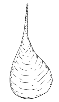
Figure 4: The incoming and outgoing plane waves. The plane wave $e^{-ip\tilde{y}}$ incoming from infinity of the $y$ axis, the vertex ${\cal D}$, elastically scatters on the boundary $ACB$ of the fundamental triangle ${\cal F}$ on Fig. 3, the bottom of the Artin surface $\bar{{\cal F}}$. The reflection amplitude $\theta(\frac{1}{2}+ip)/\theta(\frac{1}{2}-ip)$ is a pure phase and is given by the expression in front of the outgoing plane wave $e^{ip\tilde{y}}$. The rest of the wave function describes the standing waves in the $x$ direction between boundaries $x=\pm 1/2$ with the amplitudes, which are exponentially decreasing. On the right figure is an artistic image of the Artin surface, as far as it cannot be smoothly embedded into $R^{3}$.

Let us consider the geodesic flow on ${\cal F}$ described by the action (7.55)

$$S=\int ds=\int\frac{\sqrt{\dot{x}^{2}+\dot{y}^{2}}}{y}\,\,dt~{}$$ (8.105)

and the equations of motion

$$\frac{d}{dt}\,\,\frac{\dot{x}}{\,y\sqrt{\dot{x}^{2}+\dot{y}^{2}}}=0,~{}~{}~{}~{}~{}~{}~{}~{}\frac{d}{dt}\,\,\frac{\dot{y}}{\,y\sqrt{\dot{x}^{2}+\dot{y}^{2}}}+\frac{\sqrt{\dot{x}^{2}+\dot{y}^{2}}}{\,y^{2}}=0.$$ (8.106)

Notice the invariance of the action and of the equations under time reparametrisations $t\rightarrow t(\tau)$. The presence of this local gauge symmetry indicates that we have a constrained dynamical system [96]. A convenient gauge fixing which specifies the time parameter $t$ to be proportional to the proper time, is archived by imposing the condition

$${\dot{x}^{2}+\dot{y}^{2}\over y^{2}}=2H\,,$$ (8.107)

where $H$ is a constant. In this gauge the equations (8.106) will take the form [96]

$$\frac{d}{dt}\,\,(\frac{\dot{x}}{\,y^{2}})=0,~{}~{}~{}~{}~{}\frac{d}{dt}\,\,(\frac{\dot{y}}{\,y^{2}})+\frac{2H}{\,y}=0.$$ (8.108)

Defining the canonical momenta as $p_{x}=\frac{\dot{x}}{\,y^{2}},~{}p_{y}=\frac{\dot{y}}{\,y^{2}},$ conjugate to the coordinates $(x,y)$, one can get the geodesic equations (8.108) in the Hamiltonian form:

$$\dot{p_{x}}=0,~{}~{}~{}~{}\dot{p_{y}}=-\frac{2H}{\,y}.$$ (8.109)

The Hamiltonian will take the form

$$H={1\over 2}y^{2}(p^{2}_{x}+p^{2}_{y})$$ (8.110)

and the corresponding equations will take the following form:

$$\dot{x}=\frac{\partial H}{\,\partial p_{x}}=y^{2}p_{x},~{}\dot{y}=\frac{\partial H}{\,\partial p_{y}}=y^{2}p_{y}$$ (8.111)

$$\dot{p_{x}}=-\frac{\partial H}{\,\partial x}=0,~{}\dot{p_{y}}=-\frac{\partial H}{\,\partial y}=-y(p^{2}_{x}+p^{2}_{y})=-\frac{2H}{\,y},$$

and they coincide with (8.109). The advantage of the gauge (8.107) is that the Hamiltonian (8.110) coincides with the constraint.

Now it is fairly standard to quantize this Hamiltonian system by replacing in (8.110) $p_{x}=-i\frac{\partial}{\partial x},p_{y}=-i\frac{\partial}{\partial y}$ and considering time independent Schrödinger equation $H\psi=E\psi.$ The resulting equation explicitly reads:

$$-y^{2}(\partial_{x}^{2}+\partial_{y}^{2})\psi=E\psi.$$ (8.112)

On the lhs one easily recognises the Laplace operator [91, 92, 93, 94, 95, 97, 98, 99](with an extra minus sign) in Poincare metric (7.55). It is easy to see that the Hamiltonian is positive semi-definite Hermitian operator:

$$-\int\psi^{*}(x,y)\,y^{2}(\partial_{x}^{2}+\partial_{y}^{2})\,\psi(x,y){dxdy\over y^{2}}=\int(|\partial_{x}\psi(x,y)|^{2}+|\partial_{y}\psi(x,y)|^{2})dxdy\geq 0.~{}~{}~{}~{}$$ (8.113)

It is convenient to introduce parametrization of the energy $E=s(1-s)$ and to rewrite the Schrödinger equation as

$$-y^{2}(\partial_{x}^{2}+\partial_{y}^{2})~{}\psi(x,y)=s(1-s)~{}\psi(x,y).$$ (8.114)

As far as $E$ is real and semi-positive and parametrisation is symmetric with respect to $s\leftrightarrow 1-s$ it follows that the parameter $s$ should be chosen within the range

$$s\in[1/2,1]~{}~{}\text{or }~{}~{}s=1/2+iu,~{}~{}~{}u~{}\in~{}[0,\infty].$$ (8.115)

One should impose the ”periodic” boundary condition on the wave function with respect to the modular group

$$\psi(\frac{az+b}{cz+d})=\psi(z),~{}~{}~{}\left(\begin{array}[]{cc}a&b\\ c&d\end{array}\right)\in SL(2,Z)$$ (8.118)

in order to have the wave function which is properly defined on the fundamental region $\bar{{\cal F}}$ shown in Fig. 3 . Taking into account that the transformation $T:z\rightarrow z+1$ belongs to $SL(2,Z)$, one has to impose the periodicity condition $\psi(z)=\psi(z+1)$ and get the Fourier expansion $\psi(x,y)=\sum_{n=-\infty}^{\infty}f_{n}(y)\exp(2\pi inx).$ Inserting this into Eq. (8.114), for the Fourier component $f_{n}(y)$ one can get $\frac{d^{2}f_{n}(y)}{dy^{2}}+(s(1-s)-4\pi^{2}n^{2})f_{n}(y)=0~{}.$ For the case $n\neq 0$ the solution which exponentially decays at large $y$ reads $f_{n}(y)=\sqrt{y}K_{s-\frac{1}{2}}(2\pi n|y|)$ and for $n=0$ one simply gets $f_{0}(y)=c_{0}y^{s}+c^{{}^{\prime}}_{0}y^{1-s}.$ Thus the solution can be represented in the form [91, 92, 93, 94, 95, 97, 98, 99]

$$\psi(x,y)=c_{0}y^{s}+c^{{}^{\prime}}_{0}y^{1-s}+\sqrt{y}\sum_{n=-\infty\atop n\neq 0}^{\infty}c_{n}K_{s-\frac{1}{2}}(2\pi n|y|)\exp(2\pi inx),$$ (8.119)

where the coefficients $c_{0},c^{{}^{\prime}}_{0},c_{n}$ should be defined in such a way that the wave function will fulfil the boundary conditions (8.118). Thus one should impose also the invariance with respect to the second generator of the modular group $SL(2,Z)$, that is, with respect to the transformation $S:z\rightarrow-1/z$  : $\psi(z)=\psi(-1/z).$ This functional equation defines the coefficients $c_{0},c^{{}^{\prime}}_{0},c_{n}$. Another option is to start from a particular solution and perform summation over all nonequivalent shifts of the argument by the elements of $SL(2,Z)$, that is using the Poincaré series representation [5, 6, 91, 92, 93, 94, 95, 97, 98, 99]. Let us demonstrate this strategy by using the simplest solution (8.119) with $c_{0}=1,c^{{}^{\prime}}_{0}=0$:

$$\psi(z)=y^{s}=(\Im z)^{s}\,.$$

The $\Gamma_{\infty}$ is the subgroup of $\Gamma=SL(2,Z)$ generating shifts $z\rightarrow z+n$, $n\in Z$. Since $y^{s}$ is already invariant with respect to $\Gamma_{\infty}$, one should perform summation over the conjugacy classes $\Gamma_{\infty}\backslash\Gamma$. There is a bijection between the set of mutually prime pairs $(c,d)$ with $(c,d)\neq(0,0)$ and the set of conjugacy classes $\Gamma_{\infty}\backslash\Gamma$. The fact that the integers $(c,d)$ are mutually prime integers means that their greatest common divisor (gcd) is equal to one: $gcd(c,d)=1$. As a result, it is defined by the classical Poincaré series representation [5, 6] and for the sum of our interest we get

$$\psi_{s}(z)\equiv\frac{1}{2}\sum_{\gamma\in\Gamma_{\infty}\backslash\Gamma}(\Im(\gamma z))^{s}=\frac{1}{2}\sum_{(c,d)\in\mathbb{Z}^{2}\atop gcd(c,d)=1}\frac{y^{s}}{((cx+d)^{2}+c^{2}y^{2})^{s}}~{},$$ (8.120)

where, as explained above, the sum on r.h.s. is taken over all mutually prime pairs $(c,d)$. To evaluate the sum one should multiply both sides of the eq. (8.120) by $\sum_{n=1}^{\infty}\frac{1}{n^{2s}}\equiv\zeta(2s)$ [91] so that the wave function will be expressed in terms of the Eisenstein series:

$$\zeta(2s)\,\psi_{s}(z)=\frac{1}{2}\sum_{(m,k)\in\mathbb{Z}^{2}\atop(m,k)\neq(0,0)}\frac{y^{s}}{((mx+k)^{2}+m^{2}y^{2})^{s}}.$$ (8.121)

The evaluation of the sum can be now performed explicitly, and it allows to represent the (8.121) in the following form:

$$\zeta(2s)\,\psi_{s}(x,y)=\zeta(2s)y^{s}+\frac{\sqrt{\pi}\Gamma(s-\frac{1}{2})\zeta(2s-1)}{\Gamma(s)}\,y^{1-s}+$$

$$+\sqrt{y}\frac{4\pi^{s}}{\Gamma(s)}\sum_{l=1}^{\infty}\tau_{s-\frac{1}{2}}(l)K_{s-\frac{1}{2}}(2\pi ly)\cos(2\pi lx),$$ (8.122)

where the modified Bessel’s $K$ function is given by the expression $K_{iu}(y)={1\over 2}\int^{\infty}_{-\infty}e^{-y\cosh t}e^{iut}dt$ and $\tau_{ip}(n)=\sum_{a\cdot b=n}\left(\frac{a}{b}\right)^{ip}.$ By using Riemann’s reflection relation

$$\zeta(s)=\frac{\pi^{s-\frac{1}{2}}\Gamma\left(\frac{1-s}{2}\right)}{\Gamma\left(\frac{s}{2}\right)}\,\zeta(1-s)$$ (8.123)

and introducing the function

$$\theta(s)=\pi^{-s}\zeta(2s)\Gamma(s)$$ (8.124)

we get an elegant expression of the eigenfunctions obtained by Maass [91]:

$$\theta(s)\psi_{s}(z)=\theta(s)y^{s}+\theta(1-s)\,y^{1-s}+4\sqrt{y}\sum_{l=1}^{\infty}\tau_{s-\frac{1}{2}}(l)K_{s-\frac{1}{2}}(2\pi ly)\cos(2\pi lx).\qquad$$ (8.125)

This wave function is well defined in the complex $s$ plane and has a simple pole at $s=1$. The physical continuous spectrum was defined in (8.115), where $s=\frac{1}{2}+iu$, $u\in[0,\infty]$, therefore

$$E=s(1-s)=\frac{1}{4}+u^{2}.$$ (8.126)

The continuous spectrum wave functions $\psi_{s}(x,y)$ are delta function normalisable [91, 92, 93, 94, 97, 95]. The wave function (8.125) can be conveniently represented also in the form

$$\psi_{\frac{1}{2}+iu}(z)=y^{\frac{1}{2}+iu}+{\theta(\frac{1}{2}-iu)\over\theta(\frac{1}{2}+iu)}\,y^{\frac{1}{2}-iu}+{4\sqrt{y}\over\theta(\frac{1}{2}+iu)}\sum_{l=1}^{\infty}\tau_{iu}(l)K_{iu}(2\pi ly)\cos(2\pi lx),$$ (8.127)

where $K_{-iu}(y)=K_{iu}(y),~{}~{}~{}~{}~{}\tau_{-iu}(l)=\tau_{iu}(l)~{}.$ The physical interpretation of the wave function becomes more transparent if one introduce the new variables

$$\tilde{y}=\ln y,~{}~{}~{}~{}p=-u,~{}~{}~{}~{}E=p^{2}+\frac{1}{4},$$ (8.128)

as well as the alternative normalisation of the wave function $\psi_{p}(x,\tilde{y})\equiv y^{-\frac{1}{2}}\psi_{\frac{1}{2}+iu}(z)$

$$\psi_{p}(x,\tilde{y})=e^{-ip\tilde{y}}+{\theta(\frac{1}{2}+ip)\over\theta(\frac{1}{2}-ip)}\,e^{+ip\tilde{y}}+{4\over\theta(\frac{1}{2}-ip)}\sum_{l=1}^{\infty}\tau_{ip}(l)K_{ip}(2\pi le^{\tilde{y}})\cos(2\pi lx).$$ (8.129)

The first two terms describe the incoming and outgoing plane waves. The plane wave $e^{-ip\tilde{y}}$ incoming from infinity of the $y$ axis on Fig.4 ( the vertex ${\cal D}$) elastically scatters on the boundary $ACB$ of the fundamental region ${\cal F}$. The reflection amplitude is a pure phase and is given by the expression in front of the outgoing plane wave $e^{ip\tilde{y}}$

$${\theta(\frac{1}{2}+ip)\over\theta(\frac{1}{2}-ip)}=\exp{[i\,\varphi(p)]}.$$ (8.130)

The rest of the wave function describes the standing waves $\cos(2\pi lx)$ in the $x$ direction between boundaries $x=\pm 1/2$ with the amplitudes $K_{ip}(2\pi ly)$, which are exponentially decreasing with index $l$.

In addition to the continuous spectrum the system (8.114) has a discrete spectrum [91, 92, 93, 94, 97, 95]. The number of discrete states is infinite: $E_{0}=0<E_{1}<E_{2}<....\rightarrow\infty$, the spectrum is extended to infinity - unbounded from above - and lacks any accumulation point except infinity. The wave functions of the discrete spectrum have the form [91, 92, 93, 94, 104, 100, 101]

$$\psi_{n}(z) = \sum_{l=1}^{\infty}c_{l}(n)\,\sqrt{y}\,K_{iu_{n}}(2\pi ly)\left\{\begin{array}[]{ll}\cos(2\pi lx)\\ \sin(2\pi lx)\\ \end{array}\right.,$$ (8.133)

where the spectrum $E_{n}={1\over 4}+u^{2}_{n}$ and the coefficients $c_{l}(n)$ are not known analytically, but were computed numerically for many values of $n$ [104, 100, 101]. Having explicit expressions of the wave functions one can analyse the quantum-mechanical behaviour of the correlation functions, which we shall investigate in the next sections.

9 Quantum Mechanical Correlation Functions

The two-point correlation function is defined as:

$${\cal D}_{2}(\beta,t)=\langle A(t)B(0)e^{-\beta H}\rangle=\sum_{n}\langle n|e^{iHt}A(0)e^{-iHt}B(0)e^{-\beta H}|n\rangle=$$

$$=\sum_{n,m}e^{i(E_{n}-E_{m})t-\beta E_{n}}\langle n|A(0)|m\rangle\langle m|B(0)|n\rangle.$$ (9.134)

The energy eigenvalues (8.126) are parametrised by $n={1\over 2}+iu$, $E_{n}=\frac{1}{4}+u^{2}$ and $m={1\over 2}+iv$, $E_{m}=\frac{1}{4}+v^{2}$, thus [11]

$${\cal D}_{2}(\beta,t)=\int^{+\infty}_{0}\int^{+\infty}_{0}du\,dv~{}e^{i(u^{2}-v^{2})t-\beta(\frac{1}{4}+u^{2})}$$ (9.135)

$$\int_{{\cal F}}\psi_{\frac{1}{2}-iu}(z)\,A\,\psi_{\frac{1}{2}+iv}(z)\,d\mu(z)\int_{{\cal F}}\psi_{\frac{1}{2}-iv}(w)\,B\,\psi_{\frac{1}{2}+iu}(w)\,d\mu(w)~{},$$

where the complex conjugate function is $\psi^{*}_{\frac{1}{2}+iu}(z)=\psi_{\frac{1}{2}-iu}(z)$. Defining the basic matrix element as

$$A_{uv}=\int_{{\cal F}}\psi_{\frac{1}{2}-iu}(z)\,A\,\psi_{\frac{1}{2}+iv}(z)\,d\mu(z)=\int^{1/2}_{-1/2}dx\int^{\infty}_{\sqrt{1-x^{2}}}{dy\over y^{2}}\psi_{\frac{1}{2}-iu}(z)\,A\,\psi_{\frac{1}{2}+iv}(z)$$ (9.136)

for the two-point correlation function one can get

$${\cal D}_{2}(\beta,t)=\int^{+\infty}_{-\infty}e^{i(u^{2}-v^{2})t-\beta(\frac{1}{4}+u^{2})}A_{uv}\,B_{vu}\,dudv.~{}~{}~{}$$ (9.137)

In terms of the new variables (8.128) the basic matrix element (9.136) will take the form

$$A_{pq}=\int^{1/2}_{-1/2}dx\int^{\infty}_{{1\over 2}\log(1-x^{2})}dy\psi^{*}_{p}(x,y)\,(e^{-\frac{1}{2}y}A\,e^{\frac{1}{2}y})\,\psi_{q}(x,y).~{}~{}~{}~{}~{}$$ (9.138)

The matrix element (9.136), (9.138) plays a fundamental role in the investigation of the correlation functions because all correlations can be expressed through it. One should choose also appropriate observables $A$ and $B$. The operator $y^{-2}$ seems very appropriate for two reasons. Firstly, the convergence of the integrals over the fundamental region ${\cal F}$ will be well defined. Secondly, this operator is reminiscent of the exponentiated Louiville field since $y^{-2}=e^{-2\tilde{y}}$ . Thus the interest is in calculating the matrix element (9.138) for the observables in the form of the Louiville-like operators [11]:

$$A(N)=e^{-2Ny}$$ (9.139)

with matrix element

$$A_{pq}(N)=\int^{1/2}_{-1/2}dx\int^{\infty}_{{1\over 2}\log(1-x^{2})}dy~{}\psi^{*}_{p}(x,y)\,e^{-2Ny}\,\psi_{q}(x,y),$$

$$~{}~{}N=1,2,...$$ (9.140)

The other interesting observable is $A=\cos(2\pi Nx),N=1,2,...$. The evaluation of the above matrix elements is convenient to perform using a perturbative expansion in which the part of the wave function (8.129) containing the Bessel’s functions and the contribution of the discrete spectrum (8.133) is considered as a perturbation. These terms of the perturbative expansion are small and don’t change the physical behaviour of the correlation functions. The reason behind this fact is that in the integration region $\Im z\gg 1,\Im w\gg 1$ of the matrix element (9.136) the Bessel’s functions decay exponentially. Therefore the contribution of these high modes is small (analogues to the so called mini-superspace approximation in the Liouville theory). In the first approximation of the wave function (8.129) for the matrix element one can get [11]

$$A_{pq}(N)={\,{}_{2}F_{1}\left(\frac{1}{2},N+i{p-q\over 2};\frac{3}{2};\frac{1}{4}\right)\over 2N+i(p-q)}+{\,{}_{2}F_{1}\left(\frac{1}{2},N+i{p+q\over 2};\frac{3}{2};\frac{1}{4}\right)\over 2N+i(p+q)}e^{-i\varphi(q)}$$

$$+{\,{}_{2}F_{1}\left(\frac{1}{2},N-i{p+q\over 2};\frac{3}{2};\frac{1}{4}\right)\over 2N-i(p+q)}e^{i\varphi(p)}+{\,{}_{2}F_{1}\left(\frac{1}{2},N-i{p-q\over 2};\frac{3}{2};\frac{1}{4}\right)\over 2N+i(p-q)}e^{i(\varphi(p)-\varphi(q))},$$ (9.141)

where the reflation phase $\varphi(p)$ was defined in (8.130). Thus

$${\cal D}_{2}(\beta,t)=\int^{+\infty}_{-\infty}e^{i(p^{2}-q^{2})t-\beta(\frac{1}{4}+p^{2})}A_{pq}(N)\,A_{qp}(M)\,dpdq~{}.$$ (9.142)

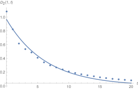
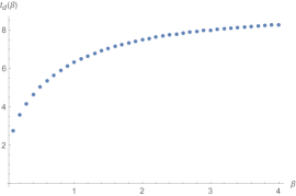
Figure 5: The exponential decay of the two-point correlation function ${\cal D}_{2}(\beta,t)$ as a function of time at temperature $\beta=1$. The points are fitted by the curve $K(\beta)\exp{(-t/t_{d}(\beta))}$. The exponent $t_{d}(\beta)$ has a well defined high and low temperature limits. The limiting values in dimensionless units are $t_{d}(0)\approx 0.276$ and $t_{d}(\infty)\approx 0.749$. The temperature dependence of $K(\beta)$ is shown on the l.h.s. graph.

The correlation function is for two Louiville-like fields in the power $N$ and $M$ respectively. This expression is very convenient for the analytical and numerical analyses. It is expected that the two-point correlation function decay exponentially [40]

$${\cal D}_{2}(\beta,t)\sim K(\beta)~{}e^{-{t\over t_{d}(\beta)}},$$ (9.143)

where $t_{d}(\beta)$ is the decorrelation time and defines one of the characteristic time scales in the quantum-mechanical system. The exponential decay of the two-point correlation function with time at different temperatures is shown on Fig.5. The dependence of the exponent $t_{d}(\beta)$ and of the prefactor $K(\beta)$ as a function of temperature are presented in Fig.5. As one can see, at high and low temperatures the decorrelation time tends to the fixed values. The corresponding limiting values in dimensionless units are shown on the Fig.5.

It was conjectured in the literature [40] that the classical chaos can be diagnosed in thermal quantum systems by using an out-of-time-order correlation functions as well as by the square of the commutator of the operators which are separated in time. The out-of-time four-point correlation function of interest was defined in [40] as follows:

$${\cal D}_{4}(\beta,t)=\langle A(t)B(0)A(t)B(0)e^{-\beta H}\rangle=\sum_{n,m,l,r}e^{i(E_{n}-E_{m}+E_{l}-E_{r})t-\beta E_{n}}$$

$$\langle n|A(0)|m\rangle\langle m|B(0)|l\rangle\langle l|A(0)|r\rangle\langle r|B(0)|n\rangle.$$

The other important observable is the square of the commutator of the Louiville-like operators separated in time [40]

$$C(\beta,t)=\langle[A(t),B(0)]^{2}e^{-\beta H}\rangle~{}.$$ (9.144)

The energy eigenvalues we shall parametrise as $n={1\over 2}+iu$, $m={1\over 2}+iv$,$l={1\over 2}+il$ and $r={1\over 2}+ir$, thus from (9) we shall get [11]

$${\cal D}_{4}(\beta,t)=\int^{+\infty}_{-\infty}e^{i(u^{2}-v^{2}+l^{2}-r^{2})t-\beta(\frac{1}{4}+u^{2})}A_{uv}\,B_{vl}\,A_{lr}\,B_{ru}\,dudvdldr~{}.$$ (9.145)

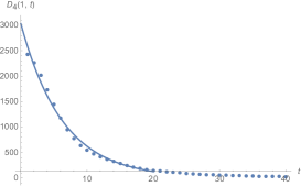
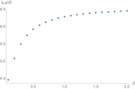
Figure 6: The exponential decay of the correlation function ${\cal D}_{4}(\beta,t)$ as a function of time at $\beta=1$. The rest of the functions ${\cal D}^{\prime}_{4}(\beta,t),{\cal D}^{\prime\prime}_{4}(\beta,t),{\cal D}^{\prime\prime\prime}_{4}(\beta,t)$ demonstrate a similar exponential decay $\sim~{}\exp{(-{t\over t_{4d}(\beta)})}$. The temperature dependence of the exponent $t_{4d}(\beta)$ has a well defined high and low temperature limits and is shown on the r.h.s. graph. The corresponding limiting values of the function $t_{4d}(\beta)$ in dimensionless units are $t_{4d}(0)=0,112$ and $t_{4d}(\infty)=0,163$. The behaviour of the exponent $t_{d}(\beta)$ of the two-point correlation function is shown on the Fig.5.

In terms of the variables (8.128) the four-point correlation function (9.145) will take the following form:

$${\cal D}_{4}(\beta,t)=\int^{+\infty}_{-\infty}e^{i(p^{2}-q^{2}+l^{2}-r^{2})t-\beta(\frac{1}{4}+p^{2})}A_{pq}(N)\,A_{ql}(M)\,A_{lr}(N)\,A_{rp}(M)\,dpdqdldr.~{}~{}~{}~{}~{}~{}~{}~{}$$ (9.146)

As it was suggested in [40], the most important correlation function indicating the traces of the classical chaotic dynamics in quantum regime is (9.144)

$$C(\beta,t)=-{\cal D}_{4}(\beta,t)+{\cal D}^{\prime}_{4}(\beta,t)+{\cal D}^{\prime\prime}_{4}(\beta,t)-{\cal D}^{\prime\prime\prime}_{4}(\beta,t).$$ (9.147)

In the case of the Artin system one can get [11]

$${\cal D}^{\prime}_{4}(\beta,t)+{\cal D}^{\prime\prime}_{4}(\beta,t)=2\int^{+\infty}_{-\infty}e^{-\beta(\frac{1}{4}+p^{2})}~{}\cos{(q^{2}-r^{2})t}$$

$$~{}~{}~{}~{}~{}~{}~{}~{}~{}~{}~{}~{}~{}~{}~{}~{}~{}A_{pq}(N)\,A_{ql}(M)\,A_{lr}(N)\,A_{rp}(M)\,dpdqdldr$$ (9.148)

and

$${\cal D}_{4}(\beta,t)+{\cal D}^{\prime\prime\prime}_{4}(\beta,t)=2\int^{+\infty}_{-\infty}e^{-\beta(\frac{1}{4}+p^{2})}~{}\cos{(p^{2}-q^{2}+l^{2}-r^{2})t}$$

$$~{}~{}~{}~{}~{}~{}~{}~{}~{}~{}~{}~{}~{}~{}~{}~{}~{}A_{pq}(N)\,A_{ql}(M)\,A_{lr}(N)\,A_{rp}(M)\,dpdqdldr.$$ (9.149)

The Fig.6 shows the behaviour of the four-point correlation ${\cal D}_{4}(\beta,t)$ as the function of the temperature and time. All four correlation functions decay exponentially:

$${\cal D}_{4}(\beta,t)\sim K(\beta)~{}e^{-{t\over t_{4d}(\beta)}}.$$ (9.150)

The four-point correlation functions ${\cal D}_{4}(\beta,t)$ do not have a simple exprssion in terms of the two-point correlation functions ${\cal D}_{2}(\beta,t)$, as one can see from the data presented on Fig.5 and Fig.6.

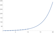
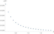
Figure 7: Time evolution of the correlation function $C(\beta,t)$ (9) at temperature $\beta=0.1$. For the short time intervals the function $C(\beta,t)$ exponentially increases with time. This behaviour is reminiscent to the exponential divergency of the classical trajectories in hyperbolic dynamical systems. As one can see, the exponent $\chi(\beta)$ which defines the behaviour of the correlation function of the operators separated in time in the commutator (9), (9.153) slowly decreases with $\beta$. Such behaviour of the correlation function $C(\beta,t)$ does not saturate the maximal growth future (9.152) which is linear in $\beta$.

Turning to the investigation of the commutator (9.144), (9.147) it is convenient to represent it in the following form [11]:

$$C(\beta,t)=2\int^{+\infty}_{-\infty}e^{-\beta(\frac{1}{4}+p^{2})}~{}\{\cos{(q^{2}-r^{2})t}-\cos{(p^{2}-q^{2}+l^{2}-r^{2})t}\}$$

$$A_{pq}(N)\,A_{ql}(M)\,A_{lr}(N)\,A_{rp}(M)\,dpdqdldr,$$ (9.151)

where (9) and (9) have been used. It was conjectured in [40] that the influence of chaos on the commutator $C(\beta,t)$ can develop no faster than exponentially:

$$C(\beta,t)\approx f(\beta)\,e^{{2\pi\over\beta}t},~{}~{}$$ (9.152)

with the exponent ${2\pi\over\beta}t=2\pi Tt$, which is growing linear in temperature $1/\beta=T$ and time $t$. Calculating the function $C(\beta,t)$ one can check if in case of classically chaotic Artin system the grows is exponential:

$$C(\beta,t)\sim f(\beta)\,e^{{2\pi\over\chi(\beta)}t},$$ (9.153)

and if the exponent $\chi(\beta)$ grows linearly with $\beta$.

The results of the integration are presented on the Fig.7. This beautifully confirms the fact that the correlation function $C(\beta,t)$ indeed grows exponentially with time as it takes place in its classical counterpart. As one can see, the exponent $\chi(\beta)$ defining the behaviour of the commutator $C(\beta,t)$ in (9) and (9.153) slowly decreases with $\beta$. Such behaviour of the commutator $C(\beta,t)$ does not saturate the maximal growth of the correlation function which is linear in $\beta$.

In order to check if the results are sensitive to the truncation of the high modes of the Maass wave function (8.125) one can include the high modes into the integration of the basic matrix element $A_{uv}$ in (9.136). It has been found that their influence on the behaviour of the correlation functions is negligible. The numerical values of the exponents $t(\beta)$ and $\chi(\beta)$ are changing in the range of few percentage and do not influence the results. In summary, all two and four-point correlation functions decay exponentially. The commutator $C(\beta,t)$ in (9) and (9.153) grows exponentially with exponent which is almost constant Fig.7. This behaviour does not saturate the condition of the maximal growth (9.152).

10 Artin Resonances and Riemann Zeta Function Zeros

Here we shall demonstrate that the Riemann zeta function zeros define the position and the widths of the resonances of the quantised Artin dynamical system [12]. As it was discussed in previous sections the Artin dynamical system is defined on the fundamental region of the modular group on the Lobachevsky plane. It has a finite area and an infinite extension in the vertical direction that correspond to a cusp Fig.8. In classical regime the geodesic flow on this non-compact surface of constant negative curvature represents one of the most chaotic dynamical systems, has mixing of all orders, Lebesgue spectrum and non-zero Kolmogorov entropy. In quantum-mechanical regime the system can be associated with the narrow infinitely long waveguide stretched out to infinity along the vertical axis and a cavity resonator attached to it at the bottom. That suggests a physical interpretation of the Maass automorphic wave function in the form of an incoming plane wave of a given energy entering the resonator, bouncing and scattering to infinity. As the energy of the incoming wave comes close to the eigenmodes of the cavity a pronounced resonance behaviour shows up in the scattering amplitude [12].

Figure 8: The Arin system is defined on a non-compact surface $\bar{{\cal F}}$ of constant negative curvature which has a topology of sphere with a cusp on the north pole which is stretched to infinity. The deficit angles on the vertices of the Artin surface can be computed using the formula $2\pi-\alpha$, thus $\int K\sqrt{g}d^{2}\xi=(-1){\pi\over 3}+(2\pi-2{\pi\over 3})+(2\pi-2{\pi\over 2})+(2\pi-0)=4\pi$.

We already presented above (8.129) the Maass wave function [91] in terms of the natural physical variable $\tilde{y}$, which is the distance in the vertical direction on the Lobachevsky plane $\ln y=\tilde{y}$, and of the corresponding momentum $p$ [11]. The plane wave $e^{-ip\tilde{y}}$ incoming from infinity ${\cal D}$ of the $y$ axis on Fig.3, Fig.4 and Fig.8 elastically scatters on the boundary $ACB$ of the fundamental triangle ${\cal F}$. The reflection amplitude is a pure phase and is given by the expression in front of the outgoing plane wave $e^{ip\tilde{y}}$ :

$$S={\theta(\frac{1}{2}+ip)\over\theta(\frac{1}{2}-ip)}=\exp{[2\,i\,\delta(p)]}.$$ (10.154)

The other terms of the wave function describes the standing waves $\cos(2\pi lx)$ in the $x$ direction between the boundaries $x=\pm 1/2$ with the amplitudes $K_{ip}(2\pi le^{\tilde{y}})$, which are exponentially decreasing with index $l$. The continuous energy spectrum is given by the formula [11]

$$E=p^{2}+\frac{1}{4}.$$ (10.155)

In physical terms the system can be described as a narrow infinitely long waveguide stretched out to infinity along the vertical dierection and a cavity resonator attached to it at the bottom $ACB$ (see Fig.4 and Fig.8). In order to support this interpretation we can calculate the area of the Artin surface which is below the fixed coordinate $y_{0}=e^{\tilde{y}_{0}}$:

$$\text{Area}({\cal F}_{0})=\int_{-\frac{1}{2}}^{\frac{1}{2}}dx\int_{\sqrt{1-x^{2}}}^{y_{0}}\frac{dy}{y^{2}}=\frac{\pi}{3}-2e^{-\tilde{y}_{0}}\,=\text{Area}({\cal F})-e^{-\tilde{y}_{0}}\,,$$ (10.156)

and confirm that the area above the ordinate $\tilde{y}_{0}$ is exponentially small: $e^{-\tilde{y}_{0}}$. The horizontal ( $dy=0$) size of the Artin surface also decreases exponentially in the vertical direction:

$$L_{0}=2\int ds=2\int\frac{\sqrt{dx^{2}+dy^{2}}}{y}=\int_{-\frac{1}{2}}^{\frac{1}{2}}{dx\over y_{0}}=e^{-\tilde{y}_{0}}.$$ (10.157)

One can suggest therefore the following physical interpretation of the Maass wave function (8.129): The incoming plane wave $e^{-ip\tilde{y}}$ of energy $E=p^{2}+\frac{1}{4}$ enters the ”cavity resonator”, bouncing back into the outgoing plane wave at infinity $e^{ip\tilde{y}}$. As the energy of the incoming wave $E=p^{2}+\frac{1}{4}$ close to the eigenmodes of the cavity resonator one should expect a pronounced resonance behaviour of the scattering amplitude [12].

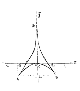
Figure 9: The system can be described as a narrow (10.157) infinitely long waveguide stretched to infinity along the vertical dierection and a cavity resonator attached to it at the bottom $ACB$.

To trace such behaviour let us consider the analytical continuation of the Maass wave function (8.129) to the complex energies $E$. The analytical continuation of the scattering amplitudes as a function of the energy $E$ considered as a complex variable allows to establish important spectral properties of the quantum-mechanical system. In particular, the method of analytic continuation allows to determine the real and complex S-matrix poles. The real poles on the physical sheet correspond to the discrete energy levels and the complex poles on the second sheet below the cut correspond to the resonances in the quantum-mechanical system [106] . The asymptotic form of the wave function can be represented in the following form:

$$\psi=A(E)\,e^{ip\tilde{y}}+B(E)\,e^{-ip\tilde{y}},~{}~{}~{}p=\sqrt{E-1/4}.$$ (10.158)

In order to make the functions $A(E)$ and $B(E)$ single-valued one should cut the complex plane along the real axis [106] starting from $E=1/4$. The complex plane with a cut so defined a physical sheet. To the left from the cut, at energies $E_{0}<1/4$, the wave function takes the following form:

$$\psi=A(E)\,e^{-\sqrt{|E-1/4|}\tilde{y}}+B(E)\,e^{\sqrt{|E-1/4|}\tilde{y}},$$ (10.159)

where the exponential factors are real and one of them decreases and the other one increases at $\tilde{y}\rightarrow\infty$. The bound states are characterised by the fact that the corresponding wave function tends to zero at infinity $\tilde{y}\rightarrow\infty$. This means that the second term in (10.159) should be absent, and a discrete energy level $E_{0}<1/4$ corresponds to a zero of the $B(E)$ function [106]:

$$B(E_{0})=0.~{}~{}~{}$$ (10.160)

Because the energy eigenvalues are real, all zeros of $B(E)$ on the physical sheet are real. Now consider a system which is unbounded and its energy spectrum has a continuous part [106]. The energy spectrum can be quasi-discrete, consisting of smeared levels of a width $\Gamma$. In describing such states one should describe the wave packet moving to infinity, thus only outgoing waves should be presence at infinity. This boundary condition involves complex quantities and the energy eigenvalues in general are also complex [106]. With such boundary conditions the Hermitian energy operators can have complex eigenvalues of the form [106]

$$E=E_{0}-i{\Gamma\over 2},$$ (10.161)

where $E_{0}$ and $\Gamma$ are both real and positive.

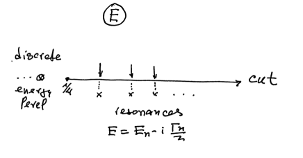
Figure 10: The resonances $E_{n}-i{\Gamma_{n}\over 2}$ are located under the right hand side of the real axis.

The condition which defines the complex energy eigenvalues (10.161) reduces to the requirement that at $E=E_{0}-i{\Gamma\over 2}$ the incoming wave $e^{-ip\tilde{y}}$ in (10.158) should be absent [106]:

$$B(E_{0}-i{\Gamma\over 2})=0.$$ (10.162)

The point $E_{0}-i{\Gamma\over 2}$ is located under the right hand side of the real axis, see Fig.13. In order to reach that point without leaving the physical sheet one should move from the upper side of the cut anticlockwise. However in that case, the phase of the wave function changes its sign and the outgoing wave transforms into the incoming wave. In order to keep the outgoing character of the wave function one should cross the cut strait into the second sheet Fig.13. Expanding the function $B(E)$ near the quasi-discrete energy level (10.161) as $B(E)=(E-E_{0}+{i\Gamma\over 2})b+...$ one can get

$$\psi~{}~{}\approx~{}~{}b^{*}(E-E_{0}-{i\Gamma\over 2})e^{ip\tilde{y}}+b(E-E_{0}+{i\Gamma\over 2})e^{-ip\tilde{y}}$$ (10.163)

and the S-matrix will take the following form [106]

$$S=e^{2i\delta}={E-E_{0}-i\Gamma/2\over E-E_{0}+i\Gamma/2}e^{2i\delta_{0}},$$ (10.164)

where $e^{2i\delta_{0}}=b^{*}/b$. One can observe that moving throughout the resonance region the phase is changing by $\pi$.

Let us now consider the asymptotic behaviour of the wave function (8.129) at large $\tilde{y}$. The conditions (10.160) and (10.162) of the absence of incoming wave takes the form [12]:

$$\theta(\frac{1}{2}-ip)=0$$ (10.165)

and due to (8.124):

$$\theta(\frac{1}{2}-ip)={\zeta(1-2ip)\Gamma(\frac{1}{2}-ip)\over\pi^{\frac{1}{2}-ip}}=0.$$ (10.166)

The solution of this equation can be expressed in terms of zeros of the Riemann zeta function [4]:

$$\zeta(\frac{1}{2}-iu_{n})=0,~{}~{}~{}~{}n=1,2,....~{}~{}~{}~{}u_{n}>0.$$ (10.167)

Thus one should solve the equation

$$1-2ip_{n}=\frac{1}{2}-iu_{n}~{}.$$ (10.168)

The location of poles is therefore at the following values of the complex momenta

$$p_{n}={u_{n}\over 2}-i\,{1\over 4}\,,~{}~{}~{}~{}~{}n=1,2,.....$$ (10.169)

and at the corresponding complex energies (10.155) :

$$E=p^{2}_{n}+{1\over 4}~{}=~{}({u_{n}\over 2}-\,{1\over 4}\,i)^{2}+{1\over 4}~{}=~{}{u^{2}_{n}\over 4}+{3\over 16}-i\,{u_{n}\over 4}.$$ (10.170)

Thus one can observe that there are resonances (10.161)

$$E=E_{n}-i{\Gamma_{n}\over 2}$$ (10.171)

at the following energies and of the corresponding widths (10.170) [12]:

$$E_{n}={u^{2}_{n}\over 4}+{3\over 16},~{}~{}~{}~{}~{}~{}\Gamma_{n}={u_{n}\over 2}.$$ (10.172)

The ratio of the width to the energy tends to zero [4]:

$${\Gamma_{n}\over E_{n}}={u_{n}\over 2}/({u^{2}_{n}\over 4}+{3\over 16})\approx{2\over u_{n}}\rightarrow~{}~{}0$$ (10.173)

and the resonances become infinitely narrow. The ratio of the width to the energy spacing between nearest levels is

$${\Gamma_{n}\over E_{n+1}-E_{n}}={2u_{n}\over(u_{n+1}+u_{n})(u_{n+1}-u_{n})}\approx{1\over u_{n+1}-u_{n}}.$$ (10.174)

As far as the zeros of the zeta function have the property to ”repel”, the difference $u_{n+1}-u_{n}$ can vanish with small probability [107, 108]. One can conjecture the following representation of the S-matrix (10.154):

$$S=e^{2i\,\delta}={\theta(\frac{1}{2}+ip)\over\theta(\frac{1}{2}-ip)}=\sum^{\infty}_{n=1}{E-E_{n}-i\Gamma_{n}/2\over E-E_{n}+i\Gamma_{n}/2}~{}e^{2i\delta_{n}}$$ (10.175)

with yet unknown phases $\delta_{n}$. In order to justify the above representation of the S-matrix one can find the location of the poles on the second Riemann sheet by using expansion of the S-matrix (10.154) at the ”bumps” which occur along the real axis at energies

$$E_{n}={u^{2}_{n}\over 4}+{3\over 16}~{}.$$ (10.176)

The expantion will take the following form:

$$S|_{E\approx E_{n}} = {\theta(\frac{1}{2}+i\sqrt{E-{1\over 4}})\over\theta(\frac{1}{2}-i\sqrt{E-{1\over 4}})}|_{E\approx E_{n}}~{}=~{}{\theta(\frac{1}{2}+i\sqrt{E_{n}-{1\over 4}})+\theta^{{}^{\prime}}(\frac{1}{2}+i\sqrt{E_{n}-{1\over 4}})~{}(E-E_{n})\over\theta(\frac{1}{2}-i\sqrt{E_{n}-{1\over 4}})+\theta^{{}^{\prime}}(\frac{1}{2}-i\sqrt{E_{n}-{1\over 4}})~{}(E-E_{n})}$$

$$= {E-E_{n}+\theta(\frac{1}{2}+i\sqrt{E_{n}-{1\over 4}})/\theta^{{}^{\prime}}(\frac{1}{2}+i\sqrt{E_{n}-{1\over 4}})\over E-E_{n}+\theta(\frac{1}{2}-i\sqrt{E_{n}-{1\over 4}})/\theta^{{}^{\prime}}(\frac{1}{2}-i\sqrt{E_{n}-{1\over 4}})}~{}~{}{\theta^{{}^{\prime}}(\frac{1}{2}+i\sqrt{E_{n}-{1\over 4}})\over\theta^{{}^{\prime}}(\frac{1}{2}-i\sqrt{E_{n}-{1\over 4}})}$$

$$\equiv ~{}~{}~{}{E-E^{{}^{\prime}}_{n}-i\Gamma^{{}^{\prime}}_{n}/2\over E-E^{{}^{\prime}}_{n}+i\Gamma^{{}^{\prime}}_{n}/2}~{}~{}e^{2i\delta^{{}^{\prime}}_{n}}~{},$$

where

$$E^{{}^{\prime}}_{n}-i\Gamma^{{}^{\prime}}_{n}/2=E_{n}-{\theta(\frac{1}{2}-i\sqrt{E_{n}-{1\over 4}})\over\theta^{{}^{\prime}}(\frac{1}{2}-i\sqrt{E_{n}-{1\over 4}})},~{}~{}~{}~{}e^{2i\delta^{{}^{\prime}}_{n}}={\theta^{{}^{\prime}}(\frac{1}{2}+i\sqrt{E_{n}-{1\over 4}})\over\theta^{{}^{\prime}}(\frac{1}{2}-i\sqrt{E_{n}-{1\over 4}})},$$ (10.178)

thus

$$E^{{}^{\prime}}_{n}-E_{n}=-\Re{\theta(\frac{1}{2}-i\sqrt{E_{n}-{1\over 4}})\over\theta^{{}^{\prime}}(\frac{1}{2}-i\sqrt{E_{n}-{1\over 4}})},~{}~{}~{}~{}~{}~{}~{}~{}-i\Gamma^{{}^{\prime}}_{n}/2=-\Im{\theta(\frac{1}{2}-i\sqrt{E_{n}-{1\over 4}})\over\theta^{{}^{\prime}}(\frac{1}{2}-i\sqrt{E_{n}-{1\over 4}})}$$ (10.179)

and all quantities $E^{{}^{\prime}}_{n}$ , $\Gamma^{{}^{\prime}}_{n}/2$ and $\delta^{{}^{\prime}}_{n}$ are real. Considering the first ten zeros of the zeta function which are known numerically [107, 108] one can calculate the position of the resonances and their widths using the approximation formulas (10.179) and get convinced that the energies and the widths of the resonances given by the exact formula (10.172) and the one given by the approximation formulas (10.179) are consistent within the two precent deviation. Alternative attempts of the physical interpretation of the zeros of the Riemann zeta function, as well as the Pólya-Hilbert conjecture and further references can be found in [105].

11 C-cascades and MIXMAX Random Number Generator

In this section we shall turn our attention to the investigation of the second class of the C-K systems defined on high dimensional tori [3]. The automorphisms of a torus are generated by the linear transformation

$$x_{i}\rightarrow\sum^{n}_{j=1}T_{ij}x_{j},~{}~{}~{}~{}(mod~{}1),$$ (11.180)

where the integer matrix $T$ has a determinant equal to one $Det~{}T=1$. In order for the automorphisms of the torus (11.180) to fulfil the C-condition it is necessary and sufficient that the matrix $T$ has no eigenvalues on the unit circle. Thus the spectrum $\{\Lambda={\lambda_{1}},...,\lambda_{n}\}$ of the matrix $T$ should fulfil the following two conditions [3]:

$$1) ~{}Det~{}T={\lambda_{1}}{\lambda_{2}}....{\lambda_{n}}=1$$

$$2) |{\lambda_{i}}|\neq 1,~{}~{}~{}~{}~{}~{}~{}~{}~{}~{}~{}\forall i.$$ (11.181)

Because the determinant of the matrix $T$ is equal to one, the Liouville’s measure $d\mu=dx_{1}...dx_{m}$ is invariant under the action of $T$. The inverse matrix $T^{-1}$ is also an integer matrix because $Det~{}T=1$. Therefore $T$ is an automorphism of the torus onto itself. All trajectories with rational coordinates $(x_{1},...,x_{n})$, and only they, are periodic trajectories of the automorphisms of the torus (11.180). The above conditions (11) on the eigenvalues of the matrix $T$ are sufficient to prove that the system belongs to the class of Anosov C-systems and therefore has mixing properties defined above (2.4)- (2.8). Because the C-systems have mixing of all orders [3] it follows that the C-systems are exhibiting the decay of the correlation functions of any order. The entropy of the Anosov automorphisms on a torus (11.180), (11) can be calculate and is equal to the sum [3, 55, 56, 58, 59, 60, 61]:

$$h(T)=\sum_{|\lambda_{\beta}|>1}\ln|\lambda_{\beta}|.$$ (11.182)

Figure 11: The automorphisms on a two-torus. The a) depicts the parallel lines along the eigenvectors and b) depicts their positions after the action of the automorphism.

Thus the entropy $h(T)$ directly depends on the spectrum of the operator $T$. This fact allows to characterise and compare the chaotic properties of dynamical C-systems quantitatively computing and comparing their entropies.

A strong instability of trajectories of a dynamical C-system leads to the appearance of statistical properties in its behaviour [52]. As a result the time average $\bar{f_{N}}(x)={1\over N}\sum^{N-1}_{n=0}f(T^{n}x)$ of the function $f(x)$ on phase space $M$ behaves as a superposition of quantities which are statistically weakly dependent. Therefore for the C-systems on a torus it was demonstrated that the fluctuations of the time averages from the phase space integral $\langle f\rangle=\int_{M}f(x)dx$ multiplied by $\sqrt{N}$ have at large $N\rightarrow\infty$ the Gaussian distribution [52]:

$$\lim_{N\rightarrow\infty}\mu\bigg{\{}x:\sqrt{N}\left(\bar{f_{N}}(x)-\langle f\rangle\right)<z\bigg{\}}={1\over\sqrt{2\pi}\sigma_{f}}\int^{z}_{-\infty}e^{-{y^{2}\over 2\sigma^{2}_{f}}}dy.$$ (11.183)

The quantity $\sqrt{N}\Bigg{(}\bar{f_{N}}(x)-\langle f\rangle\Bigg{)}$ converges in distribution to the normal random variable with standard deviation $\sigma_{f}$

$$\sigma^{2}_{f}=\sum^{+\infty}_{n=-\infty}[\langle f(x)f(T^{n}x)\rangle-\langle f(x)\rangle^{2}].$$ (11.184)

We were able to express it in terms of entropy

$$\sigma^{2}_{f}=\sum^{+\infty}_{n=-\infty}{M^{2}\over 128\pi^{4}}~{}e^{-4nh(T)}={M^{2}\over 128\pi^{4}}{e^{4h(T)}+1\over e^{4h(T)}-1}.$$ (11.185)

During the Meeting Igor ask me if the C-K systems have temperature? It seems to me that in accordance with the above result one can associate the $\sigma_{f}$ with the temperature if one compare the above Gaussian distribution with Gibbs distribution $kT=\sigma_{f}$.

It follows from the Anosov results that these hyperbolic C-systems are K-systems as well and are therefore maximally chaotic. It was suggested in 1986 in [68] to use the C-K systems defined on a torus to generate high quality pseudorandom numbers for Monte-Carlo method. The modern powerful computers open a new era for the application of the Monte-Carlo Method [64, 65, 66, 67, 68, 80, 81] for the simulation of physical systems with many degrees of freedom and of higher complexity. The Monte-Carlo simulation is an important computational technique in many areas of natural sciences, and it has significant application in particle and nuclear physics, quantum physics, statistical physics, quantum chemistry, material science, among many other multidisciplinary applications. At the heart of the Monte-Carlo (MC) simulations are pseudo Random Number Generators (RNG).

Usually pseudo random numbers are generated by deterministic recursive rules [68, 64, 65, 66, 67]. Such rules produce pseudorandom numbers, and it is a great challenge to design pseudo random number generators that produce high quality sequences. Although numerous RNGs introduced in the last decades fulfil most of the requirements and are frequently used in simulations, each of them has some weak properties which influence the results [79] and are less suitable for demanding MC simulations which are performed for the high energy experiments at CERN and other research centres. The RNGs are essentially used in high energy experiments at CERN for the design of the efficient particle detectors and for the statistical analysis of the experimental data [75].

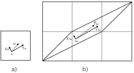
Figure 12: The tangent vector $\omega\in R_{x}$ at $x\in M^{2}$ is decomposable into the sum $R_{x}=X_{x}\bigoplus Y_{x}$ where the spaces $X_{x}$ and $Y_{x}$ are defined by the eigenvectors of the $2\times 2$ matrix $T(2,0)$ (11.186). It is exponentially contracting the distances on $X_{x}$ and expanding the distances on $Y_{x}$ (details are given in Appendix A).

In order to fulfil these demanding requirements it is necessary to have a solid theoretical and mathematical background on which the RNG’s are based. RNG should have a long period, be statistically robust, efficient, portable and have a possibility to change and adjust the internal characteristics in order to make RNG suitable for concrete problems of high complexity. In [68] it was suggested that Anosov C-systems [3], defined on a high dimensional torus, are excellent candidates for the pseudo-random number generators. The C-system chosen in [68] was the one which realises linear automorphism $T$ defined in (11.180). For convenience in this section the dimension $n$ of the phase space $M$ is denoted by $N$. A particular matrix chosen in [77] was defined for all $N\geq 2$. The operators $T(N,s)$ are parametrised by the integers $N$ and $s$

$$T(N,s)=\begin{pmatrix}1&1&1&1&...&1&1\\ 1&2&1&1&...&1&1\\ 1&3+s&2&1&...&1&1\\ 1&4&3&2&...&1&1\\ &&&...&&&\\ 1&N&N-1&N-2&...&3&2\end{pmatrix}$$ (11.186)

Its entries are all integers $T_{ij}\in\mathbb{Z}$ and $Det~{}T=1$. The spectrum and the value of the Kolmogorov entropy can be calculated.

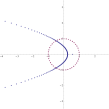
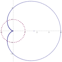
Figure 13: The eigenvalue distribution of $T(N,s)$ and of $T^{-1}(N,s)$. All eigenvalues are lying outside of the unit circle. On the r.h.s. is the MIXMAX generator implemented as the default engine into the Geant4/CLHEP toolkit at CERN.

It is defined recursively, since the matrix of size $N+1$ contains in it the matrix of the size $N$. The only variable entry in the matrix is $T_{32}=3+s$, where $s$ should be chosen such that to avoid eigenvalues lying on a unit circle. In order to generate pseudo-random vectors $x_{n}=T^{n}x$, one should choose the initial vector $x=(x_{1},...,x_{N})$, called the “seed”, with at least one non-zero component to avoid fixed point of $T$, which is at the origin. The eigenvalues of the $T$ matrix (11.186) are widely dispersed for all $N$, see Fig.13 from reference [69]. The spectrum is ”multi-scale”, with trajectories exhibiting exponential instabilities at different scales [68]. The spectrum of the operator $T(N,s)$ has two real eigenvalues for even $N$ and three for odd $N$, all the rest of the eigenvalues are complex and lying on leaf-shaped curves. It is seen that the spectrum tends to a universal limiting form as $N$ tends to infinity, and the complex eigenvalues $1/\lambda$ (of the inverse operator) lie asymptotically on the cardioid curve Fig.13 which has the representation

$$r(\phi)=4\cos^{2}(\phi/2)$$ (11.187)

in the polar coordinates $\lambda=r\exp(i\phi)$. From the above analytical expression for eigenvalues it follows that the eigenvalues satisfying the condition $0<|\lambda_{\phi}|<1$ are in the range $-2\pi/3<\phi<2\pi/3$ and the ones satisfying the condition $1<|\lambda_{\phi}|$ are in the interval $2\pi/3<\phi<4\pi/3$. One can conjecture that there exists a limiting infinite-dimensional dynamical system with continuous space coordinate and discrete time with the above spectrum. The entropy of the C-K system $T(N,s)$ can now be calculated for large values of $N$ as an integral over eigenvalues (11.187):

$$h(T)=\sum_{\alpha}\ln|{1\over\lambda_{\alpha}}|=\sum_{-2\pi/3<\phi_{i}<2\pi/3}\ln(4\cos^{2}(\phi_{i}/2)~{}\rightarrow~{}N\int^{2\pi/3}_{-2\pi/3}\ln(4\cos^{2}(\phi/2){d\phi\over 2\pi}={2\over\pi}~{}N$$ (11.188)

and to confirm that the entropy increases linearly with the dimension $N$ of the operator $T(N,s)$. In the paper [69] the period of the trajectories of the system $T(N,s)$ was found which is characterised by a prime number $p$ . In [69] the necessary and sufficient criterion were formulated for the sequence to be of the maximal possible period:

$$\tau={p^{N}-1\over p-1}\sim e^{(N-1)\ln p}.$$ (11.189)

It follows then that the period of the trajectories exponentially increases with the size of the operator $T(N,s)$. Thus the knowledge of the spectrum allows to calculate the entropy (11.188) and the period (11.189) of the trajectories. The number of periodic trajectories of a period less than $\tau$ behaves as

$$\pi(\tau)\sim\exp{({2N\tau\over\pi})}/\tau.$$ (11.190)

In summary we have the spectrum given by (11.187), the entropy by (11.188), the period on a rational sublattice by (11.189) and the corresponding density by (11.190) of the C-K system $T(N,s)$.

12 Acknowledgement

Preliminary versions of this work were presented at the Steklov Mathematical Institute (September 10, 2019) as well as the CERN Theory Department and A. Alikhanian National Laboratory in Yerevan, where part of this work was completed. I thank these institutions for their hospitality. I would like to thank Luis Alvarez-Gaume for stimulating discussions, for kind hospitality at Simons Center for Geometry and Physics and providing to the author the references [100], [101] and [99]. I would like to thank H.Babujyan, R.Poghosyan and K.Savvidy for collaboration and enlightening discussions.

13 Appendix A

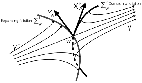
Figure 14: At each point $w$ of the C-system the tangent space $R^{m}_{w}$ is decomposable into a direct sum of two linear spaces $Y^{l}_{w}$ and $X^{k}_{w}$. The expanding and contracting geodesic flows are $\gamma^{+}$ and $\gamma^{-}$. The expanding and contracting invariant foliations $\Sigma^{l}_{w}$ and $\Sigma^{k}_{w}$ are transversal to the geodesic flows and their corresponding tangent spaces are $Y^{l}_{w}$ and $X^{k}_{w}$.

The systems with discrete time [3] is defined as a cascade on the d-dimensional compact phase space $M^{d}$ is induced by the diffeomorphisms $T:M^{d}\rightarrow M^{d}$. The iterations are defined by a repeated action of the operator $\{T^{n},-\infty<n<+\infty\}$, where $n$ is an integer number. The tangent space at the point $x\in M^{d}$ is denoted by $R^{d}_{x}$ and the tangent vector bundle by ${\cal R}(M^{d})$. The diffeomorphism $\{T^{n}\}$ induces the mapping of the tangent spaces $\tilde{T}^{n}:R^{d}_{x}\rightarrow R^{d}_{T^{n}x}$. The C-condition requires that the tangent space $R^{d}_{x}$ at each point $x$ of the d-dimensional phase space $M^{d}$ of the dynamical system $\{T^{n}\}$ should be decomposable into a direct sum of the two linear spaces $X^{k}_{x}$ and $Y^{l}_{x}$ with the following properties [3]:

$$C1. R^{d}_{x}=X^{k}_{x}\bigoplus Y^{l}_{x}~{}~{}$$ (13.191)

$$C2. ~{}~{}a)|\tilde{T}^{n}\xi|\leq~{}a|\xi|e^{-cn}~{}for~{}n\geq 0;~{}|\tilde{T}^{n}\xi|\geq~{}b|\xi|e^{-cn}~{}for~{}n\leq 0,~{}~{}~{}\xi\in X^{k}_{x},$$

$$b)|\tilde{T}^{n}\eta|\geq~{}b|\eta|e^{cn}~{}~{}for~{}n\geq 0;~{}|\tilde{T}^{n}\eta|\leq~{}a|\eta|e^{cn}~{}for~{}n\leq 0,~{}~{}~{}\eta\in Y^{l}_{x},$$

where the constants a,b and c are positive and are the same for all $x\in M^{d}$ and all $\xi\in X^{k}_{x}$, $\eta\in Y^{l}_{x}$. The length $|...|$ of the tangent vectors $\xi$ and $\eta$ is defined by the Riemannian metric on $M^{d}$. The linear spaces $X^{k}_{x}$ and $Y^{l}_{x}$ are invariant with respect to the derivative mapping $\tilde{T}^{n}X^{k}_{x}=X^{k}_{T^{n}x},~{}\tilde{T}^{n}Y^{l}_{x}=Y^{l}_{T^{n}x}$ and represent the contracting and expanding linear spaces (see Fig.14). The C-condition describes the behaviour of all trajectories $\tilde{T}^{n}\omega$ on the tangent vector bundle $\omega\in R^{d}_{x}$. Anosov proved that the vector spaces $X^{k}_{x}$ and $Y^{l}_{x}$ are continuous functions of the coordinate $x$ and that they are the target vector spaces to the foliations $\Sigma^{k}$ and $\Sigma^{l}$ which are the surfaces transversal to the trajectories $T^{n}x$ on $M^{d}$ (see Fig.14). The contracting and expanding foliations $\Sigma^{k}_{x}$ and $\Sigma^{l}_{x}$ are invariant with respect to the cascade $T^{n}$ in the sense that, under the action of these transformations a foliation transforms into a foliation [3].

14 Appendix B

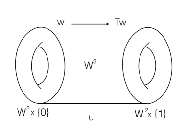
Figure 15: The identification of the $W^{2}\times\{0\}$ with $W^{2}\times\{1\}$ by the formula $(w,1)\equiv(Tw,0)$ of a cylinder $W^{2}\times[0,1]$, where $[0,1]=\{u~{}|~{}0\leq u\leq 1\}$. The resulting compact manifold $W^{3}$ has a bundle structure with the base $S^{1}$ and fibres of the type $W^{2}$. The manifold $W^{3}$ has the local coordinates $\tilde{w}=(w^{1},w^{2},u)$ .

In [3] Anosov demonstrated how any C-cascade on a torus can be embedded into a certain C-flow. The embedding was defined by the identification (14.192) and the corresponding C-flow on a smooth Riemannian manifold $W^{m+1}$ with the metric (14.199) was defined by the equations (14.194). We are interested here to analyse the geodesic flow on the same Riemannian manifold $W^{m+1}$. The geodesic flow has different dynamics (14 ) and as we shall demonstrate below has very interesting hyperbolic components different from (14.194).

Let us consider a C-cascade on a torus $W^{m}$ and increase its dimension m by one unit constructing a cylinder $W^{m}\times[0,1]$, where $[0,1]=\{u~{}|~{}0\leq u\leq 1\}$, and identifying $W^{m}\times\{0\}$ with $W^{m}\times\{1\}$ by the formula:

$$(w,1)\equiv(Tw,0).$$ (14.192)

Here T is diffeomorphism:

$$w^{i}\rightarrow\sum T_{i,j}w^{j},~{}~{}~{}~{}(mod~{}1).$$ (14.193)

The resulting compact Riemannian manifold $W^{m+1}$ has a bundle structure with the base $S^{1}$ and fibres of the type $W^{m}$. The manifold $W^{m+1}$ has the local coordinates $\tilde{w}=(w^{1},...,w^{m},u)$ shown on Fig.15. The C-flow $T^{t}$ on the manifold $W^{m+1}$ is defined by the equations [3]

$${dw^{1}\over dt}=0~{},....,~{}{dw^{m}\over dt}=0,~{}{du\over dt}=1.$$ (14.194)

For this flow the tangent space $R^{m+1}_{\tilde{w}}$ can be represented as a direct sum of three subspaces: contracting and expanding linear spaces $X^{k}_{\tilde{w}}$,$Y^{l}_{\tilde{w}}$ and $Z_{\tilde{w}}$:

$$R^{m+1}_{\tilde{w}}=X^{k}_{\tilde{w}}\oplus Y^{l}_{\tilde{w}}\oplus Z_{\tilde{w}}.$$ (14.195)

The linear space $X^{k}_{\tilde{w}}$ is tangent to the fibre $W^{m}\times u$ and is parallel to the eigenvectors corresponding to the eigenvalues which are lying inside the unit circle $0<|\lambda_{\alpha}|<1$ and $Y^{l}_{\tilde{w}}$ is tangent to the fibre $W^{m}\times u$ and is parallel to the eigenvectors corresponding to the eigenvalues which are lying outside of the unit circle $1<|\lambda_{\beta}|$. $Z_{\tilde{w}}$ is collinear to the phase space velocity (14.194). Under the derivative mapping of the (14.194) the vectors (14.201) from $X^{k}_{\tilde{w}}$ and $Y^{l}_{\tilde{w}}$ are contracting and expanding:

$$|\tilde{T}^{t}v_{1}|=\lambda_{2}^{t}~{}|v_{1}|,~{}~{}~{}~{}|\tilde{T}^{t}v_{2}|=\lambda_{1}^{t}~{}|v_{2}|.$$ (14.196)

This identification of contracting and expanding spaces proves that (14.194) indeed defines a C-flow [3].

It is also interesting to analyse the geodesic flow on a Riemannian manifold $W^{m+1}$. The equations for the geodesic flow on $W^{m+1}$

$${d^{2}\tilde{w}^{\mu}\over dt^{2}}+\Gamma^{\mu}_{\nu\rho}{d\tilde{w}^{\nu}\over dt}{d\tilde{w}^{\rho}\over dt}=0$$ (14.197)

are different from the flow equations defined by the equations (14.194) and our goal is to learn if the geodesic flow has also the properties of the C-flow. The answer to this question is not obvious and requires investigation of the curvature structure of the manifold $W^{m+1}$. If all sectional curvatures are negative then geodesic flow defines a C-flow [3]. For simplicity let us consider the automorphisms of a two-dimensional torus which is defined by the $2\times 2$ matrix $T(2,0)$ (11.186). The metric on the corresponding manifold $W^{3}$ can be defined as [26]

$$ds^{2}=e^{2u}[\lambda_{1}dw^{1}+(1-\lambda_{1})dw^{2}]^{2}+e^{2u}[\lambda_{2}dw^{1}+(1-\lambda_{2})dw^{2}]^{2}+du^{2}=\\ g_{\mu\nu}d\tilde{w}^{\mu}d\tilde{w}^{\nu},$$

where $0<\lambda_{2}<1<\lambda_{1}$ are eigenvalues of the matrix $T(2,0)$ and fulfil the relations $\lambda_{1}\lambda_{2}=1,\lambda_{1}+\lambda_{2}=3$. The metric is invariant under the transformation

$$w^{1}=2w^{{}^{\prime}1}-w^{{}^{\prime}2},~{}~{}~{}w^{2}=-w^{{}^{\prime}1}_{1}+w^{{}^{\prime}2},~{}~{}~{}u=u^{{}^{\prime}}-1$$ (14.198)

and is therefore consistent with the identification (14.192). The metric tensor has the form

$$g_{\mu\nu}(u)=\begin{pmatrix}\lambda_{1}^{2+2u}+\lambda_{2}^{2+2u}&(1-\lambda_{1})\lambda_{1}^{1+2u}+(1-\lambda_{2})\lambda_{2}^{1+2u}&0\\ (1-\lambda_{1})\lambda_{1}^{1+2u}+(1-\lambda_{2})\lambda_{2}^{1+2u}&(1-\lambda_{1})^{2}\lambda_{1}^{2u}+(1-\lambda_{2})^{2}\lambda_{2}^{2u}&0\\ 0&0&1\\ \end{pmatrix}$$ (14.199)

and the corresponding geodesic equations take the following form:

$$\ddot{w}^{1}+2{(\lambda_{1}-1)\ln\lambda_{1}\over\lambda_{1}+1}\dot{w^{1}}\dot{u}-4{(\lambda_{1}-1)\ln\lambda_{1}\over\lambda_{1}+1}\dot{w^{2}}\dot{u}=0$$

$$\ddot{w}^{2}-2{(\lambda_{1}-1)\ln\lambda_{1}\over\lambda_{1}+1}\dot{w^{2}}\dot{u}-4{(\lambda_{1}-1)\ln\lambda_{1}\over\lambda_{1}+1}\dot{w^{1}}\dot{u}=0$$ (14.200)

$$\ddot{u}+{(1-\lambda^{4u+4}_{1})\ln\lambda_{1}\over\lambda^{2u+2}_{1}}\dot{w^{1}}\dot{w^{1}}+2{(1+\lambda^{4u+3}_{1})(\lambda_{1}-1)\ln\lambda_{1}\over\lambda^{2u+2}_{1}}\dot{w^{1}}\dot{w^{2}}+$$

$$+{(1-\lambda^{4u+2}_{1})(\lambda_{1}-1)^{2}\ln\lambda_{1}\over\lambda^{2u+2}_{1}}\dot{w^{2}}\dot{w^{2}}=0.$$

One can get convinced that these equations are invariant under the transformation (14.198). In order to study a stability of the geodesic flow one has to compute the sectional curvatures. We shall choose the orthogonal frame in the directions of the linear spaces $X^{1}_{\tilde{w}},Y^{1}_{\tilde{w}}$ and $Z_{\tilde{w}}$. The corresponding vectors are:

$$v_{1}=(\lambda_{1}-1,\lambda_{1},0),~{}~{}~{}v_{2}=(\lambda_{2}-1,\lambda_{2},0),~{}~{}~{}v_{3}=(0,0,1)$$ (14.201)

and in the metric (14.199) they have the lengths:

$$|v_{1}|^{2}=(\lambda_{1}-\lambda_{2})^{2}\lambda_{2}^{2u},~{}~{}~{}~{}|v_{2}|^{2}=(\lambda_{1}-\lambda_{2})^{2}\lambda_{1}^{2u},~{}~{}~{}~{}|v_{3}|^{2}=1.$$ (14.202)

The corresponding sectional curvatures are:

$$K_{12}={R_{\mu\nu\lambda\rho}v^{\mu}_{1}v^{\nu}_{2}v^{\lambda}_{1}v^{\rho}_{2}\over|v_{1}\wedge v_{2}|^{2}}=\ln^{2}\lambda_{1}$$

$$K_{13}={R_{\mu\nu\lambda\rho}v^{\mu}_{1}v^{\nu}_{3}v^{\lambda}_{1}v^{\rho}_{3}\over|v_{1}\wedge v_{3}|^{2}}=-\ln^{2}\lambda_{2}$$ (14.203)

$$K_{23}={R_{\mu\nu\lambda\rho}v^{\mu}_{2}v^{\nu}_{3}v^{\lambda}_{2}v^{\rho}_{3}\over|v_{2}\wedge v_{3}|^{2}}=-\ln^{2}\lambda_{1}.$$

It follows from the above equations that the geodesic flow is exponentially unstable on the planes (1,3) and (2,3) and is stable in the plane (1,2). This behaviour is dual to the flow (14.194) which is unstable in (1,2) plane and is stable in (1,3) and (2,3) planes. The scalar curvature is

$$R=R_{\mu\nu\lambda\rho}g^{\mu\lambda}g^{\nu\rho}=2(K_{12}+K_{13}+K_{23})=-2\ln^{2}\lambda_{1}=-2h(T)^{2},$$ (14.204)

where $h(T)$ is the entropy of the automorphism $T(2,0)$.

15 Appendix C

In a typical computer implementation of the automorphism (14.193) the initial vector will have rational components $u_{i}=a_{i}/p$, where $a_{i}$ and $p$ are natural numbers. Therefore it is convenient to represent $u_{i}$ by its numerator $a_{i}$ in computer memory and define the iteration in terms of $a_{i}$ [78]:

$$a_{i}\rightarrow\sum_{j=1}^{N}T_{ij}\,a_{j}~{}\textrm{mod}~{}p.$$ (15.205)

If the denominator p is taken to be a prime number [78], then the recursion is realised on extended Galois field $GF[p^{N}]$ [82, 83] and allows to find the period of the trajectories in terms of p and the properties of the characteristic polynomial $P(x)$ of the matrix T [78]. If the characteristic polynomial $P(x)$ of matrix $T$ is primitive in the extended Galois field $GF[p^{N}]$, then [78, 83, 84]

$$T^{q}=p_{0}~{}\mathbb{I}~{}~{}\textrm{ where}~{}~{}q=\frac{p^{N}-1}{p-1}~{},$$ (15.206)

where $p_{0}$ is a free term of the polynomial $P(x)$ and is a primitive element of $GF[p]$. Since our matrix T has $p_{0}=DetT=1$, the polynomial $P(x)$ of T cannot be primitive. The solution suggested in [69] is to define the necessary and sufficient conditions for the period $q$ to attain its maximum are the following:

1. $T^{q}=\mathbb{I}~{}(mod~{}p)$,   where $q=\frac{p^{N}-1}{p-1}$

2. $T^{q/r}\neq\mathbb{I}~{}(mod~{}p)$,     for any r which is a prime divisor of q .

The first condition is equivalent to the requirement that the characteristic polynomial is irreducible. The second condition can be checked if the integer factorisation of $q$ is available [69], then the period of the sequence is equal to (15.206) and is independent of the seed. There are precisely $p-1$ distinct trajectories which together fill up all states of the $GF[p^{N}]$ lattice:

$$q~{}(p-1)=p^{N}-1.$$ (15.207)

In [69] the actual value of p was taken as $p=2^{61}-1$, the largest Mersenne number that fits into an unsigned integer on current 64-bit computer architectures. For the matrix of the size $N=256$ the period in that case is $q\approx 10^{4600}$. The algorithm which allows the efficient implementation of the generator in actual computer hardware, reducing the matrix multiplication to the O(N) operations was found in [69]. The other advantage of this implementation is that it allows to make ”jumps” into any point on a periodic trajectory without calculating all previous coordinates on a trajectory, which typically has a very large period $q\approx 10^{4600}$. This MIXMAX random number generator is currently made available in a portable implementation in the C language at hepforge.org [73] and was implemented into the Geant4/CLHEP and ROOT toolkits at CERN [75, 76, 74].

16 Appendix D

The most convenient way to calculate the entropy of a C-system automorphisms on a torus is to integrate over the phase space the logarithm of the volume expansion rate $\lambda(w)$ of a $l$-dimensional infinitesimal cube which is embedded into the foliation $\Sigma^{l}_{w}$. The derivative map $\tilde{T}$ maps the linear space $Y^{l}_{w}$ into the $Y^{l}_{Tw}$ and if the rate of expansion of the volume of the $l$-dimensional cube is $\lambda(w)$, then [3, 23, 54, 57, 62]

$$h(T)=\int_{W^{m}}\ln\lambda(w)dw.$$ (16.208)

Here the volume of the $W^{m}$ is normalised to 1. For the automorphisms on a torus (11.180) the coefficient $\lambda(w)$ does not depends of the phase space coordinates $w$ and is equal to the product of eigenvalues $\{\lambda_{\beta}\}$ with modulus larger than one (8.126):

$$\lambda(w)=\prod^{l}_{\beta=1}\lambda_{\beta}$$ (16.209)

and obtain the formula (11.182) for the entropy.

17 Appendix E

The entropy defines the variety and richness of the periodic trajectories of the C-systems [3, 59, 60, 61]. The C-systems have a countable set of everywhere dense periodic trajectories [3]. The $E^{m}$ cover of the torus $W^{m}$ allows to translate every set of points on torus into a set of points on Euclidean space $E^{m}$ and the space of functions on torus into the periodic functions on $E^{m}$. To every closed curve $\gamma$ on a torus corresponds a curve $\phi:[0,1]\rightarrow E^{m}$ for which $\phi(0)=\phi(1)~{}mod~{}1$ and if $\phi(1)-\phi(0)=(p_{1},...,p_{m})$, then the corresponding winding numbers on a torus are $p_{i}\in Z$.

Let us fix the integer number $N$, then the points on a torus with the coordinates having a denominator $N$ form a finite set $\{p_{1}/N,...,p_{m}/N\}$. The automorphism (11) with integer entries transform this set of points into itself, therefore all these points belong to periodic trajectories. Let $w=(w_{1},...,w_{m})$ be a point of a trajectory with the period $n>1$. Then

$$T^{n}w=w+p,$$ (17.210)

where $p$ is an integer vector. The above equation with respect to $w$ has nonzero determinant, therefore the components of $w$ are rational.

Thus the periodic trajectories of the period $n$ of the automorphism $T$ are given by the solution of the equation (17.210), where $p\in Z^{m}$ is an integer vector and $w=(w_{1},...,w_{m})\in W^{m}$. As $p$ varies in $Z^{m}$ the solutions of the equation (17.210) determine a fundamental domain $D_{n}$ in the covering Euclidian space $E^{m}$ of the volume $\mu(D_{n})=1/|Det(T^{n}-1)|$. Therefore the number of all points $N_{n}$ on the periodic trajectories of the period $n$ is given by the corresponding inverse volume [55, 56, 58, 59, 60]:

$$N_{n}=|Det(T^{n}-1)|=|\prod^{m}_{i=1}(\lambda^{n}_{i}-1)|.$$ (17.211)

Using the theorem of Bowen [60, 61] which states that the entropy of the automorphism $T$ can be represented in terms of $N_{n}$ defined in (17.211):

$$h(T)=\lim_{n\rightarrow\infty}{1\over n}~{}\ln N_{n}~{}~{},$$ (17.212)

one can derive the formula for the entropy (11.182) for the automorphism $T$ in terms of its eigenvalues:

$$h(T)=\lim_{n\rightarrow\infty}{1\over n}\ln(|\prod^{m}_{i=1}(\lambda^{n}_{i}-1)|)=\sum_{|\lambda_{\beta}|>1}\ln|\lambda_{\beta}|.$$ (17.213)

Let us now define the number of periodic trajectories of the period $n$ by $\pi(n)$. Then the number of all points $N_{n}$ on the periodic trajectories of the period $n$ can be written in the following form:

$$N_{n}=\sum_{l~{}divi~{}n}l~{}\pi(l),$$ (17.214)

where $l$ divides $n$. Using again the Bowen result (17.212) one can get

$$N_{n}=\sum_{l~{}divi~{}n}l\pi(l)\sim e^{nh(T)}.$$ (17.215)

This result can be rephrased as a statement that the number of points on the periodic trajectories of the period n exponentially grows with the entropy.

Excluding the periodic trajectories which divide n (for example $T^{n}w=T^{l_{2}}(T^{l_{1}}w)$, where $n=l_{1}l_{2}$ and $T^{l_{i}}w=w$) one can get the number of periodic trajectories of period n which are not divisible. For that one should represent the $\pi(n)$ in the following form:

$$\pi(n)={1\over n}\big{(}\sum_{l~{}divi~{}n}l~{}\pi(l)-\sum_{l~{}divi~{}n,~{}l<n}l~{}\pi(l)\big{)}$$ (17.216)

and from (17.216) and (17.215) it follows that

$$\pi(n)\sim{e^{nh(T)}\over n}\big{(}1-{\sum_{l~{}divi~{}n,~{}l<n}l~{}\pi(l)\over\sum_{l~{}divi~{}n}l~{}\pi(l)}\big{)}\sim{e^{nh(T)}\over n},$$ (17.217)

because the ratio in the bracket is strictly smaller than one. This result tells that a system with larger entropy $\Delta h=h(T_{1})-h(T_{2})>0$ is more densely populated by the periodic trajectories of the same period $n$:

$${\pi_{1}(n)\over\pi_{2}(n)}\sim e^{n\ \Delta h}.$$ (17.218)

The next important result of the Bowen theorem [60, 61] states that

$$\int_{W^{m}}f(w)d\mu(w)=\lim_{n\rightarrow\infty}{1\over N_{n}}\sum_{w\in\Gamma_{n}}f(w),$$ (17.219)

where $\Gamma_{n}$ is a set of all points on the trajectories of period $n$. The total number of points in the set $\Gamma_{n}$ we defined earlier as $N_{n}$.

This result has important consequences for the calculation of the integrals on the manifold $W^{m}$, because, as it follows from (17.219), the integration reduces to the summation over all points of periodic trajectories. It is appealing to consider periodic trajectories of the period $n$ which is a prime number. Because every infinite subsequence of convergent sequence converges to the same limit we can consider in (17.219) only terms with the prime periods. In that case $N_{n}=n\pi(n)$ and the above formula becomes:

$$\int_{W^{m}}f(w)d\mu(w)=\lim_{n\rightarrow\infty}{1\over n\pi(n)}\sum^{\pi(n)}_{j=1}\sum^{n-1}_{i=0}f(T^{i}w_{j}),$$ (17.220)

where the summation is over all points of the trajectory $T^{i}w_{j}$ and over all distinct trajectories of period n which are enumerated by index $j$. The $w_{j}$ is the initial point of the trajectory $j$ . From the above consideration it follows that the convergence is guaranteed if one sums over all trajectories of the same period $n$. One can conjecture that all $\pi(n)$ trajectories at the very large period $n$ contribute equally into the sum (17.220), therefore the integral (17.220) can be reduced to a sum over fixed trajectory

$${1\over n}\sum^{n-1}_{i=0}f(T^{i}w).$$ (17.221)

References

- [1] A.N. Kolmogorov, New metrical invariant of transitive dynamical systems and automorphisms of Lebesgue spaces, Dokl. Acad. Nauk SSSR, 119 (1958) 861-865
- [2] A.N. Kolmogorov, On the entropy per unit time as a metrical invariant of automorphism, Dokl. Acad. Nauk SSSR, 124 (1959) 754-755
- [3] D. V. Anosov, Geodesic flows on closed Riemannian manifolds with negative curvature, Trudy Mat. Inst. Steklov., Vol. 90 (1967) 3 - 210
- [4] B. Riemann Über die Anzahl der Primzahlen unter einer gegebenen Grösse, Monatsberichte der Berliner Akademie, November 1859.
- [5] Henri Poincaré Théorie des Groupes Fuchsiens, Acta Mathematica, 1 (1882) 1.
- [6] Henri Poincaré Mémoire sur les Fonctions Fuchsiennes, Acta Mathematica, 1 (1882) 193-294.
- [7] Lazarus Fuchs, Ueber eine Klasse von Funktionen mehrerer Variablen, welche durch Umkehrung der Integrale von Lösungen der linearen Differentialgleichungen mit rationalen Coeffizienten entstehen, J. Reine Angew. Math., 89 (1880) 151-169
- [8] L.R.Ford, An Introduction to the Theory of Automorphic Functions, London, 1915, Publisher G.Bell.
- [9] Emil Artin, Ein mechanisches system mit quasiergodischen bahnen, E. Abh. Math. Semin. Univ. Hambg. (1924) 3: 170.
- [10] H. R. Poghosyan, H. M. Babujian and G. K. Savvidy, Artin Billiard: Exponential Decay of Correlation Functions, Theor. Math. Phys. 197 (2018) no.2, 1592 doi:10.1134/S004057791811003X [arXiv:1802.04543 [nlin.CD]].
- [11] H. Babujian, R. Poghossian and G. Savvidy, Correlation Functions of Classical and Quantum Artin System defined on Lobachevsky Plane and Scrambling Time, arXiv:1808.02132 [hep-th].
- [12] G. Savvidy and K. Savvidy, Quantum-Mechanical interpretation of Riemann zeta function zeros, arXiv:1809.09491 [math-ph].
- [13] J. Hadamard, Sur le billiard non Euclidean, Soc. Sci. Bordeaux, Proc. Verbaux 1898, 147 (1898); J. Math Pure Appl. 4 (1898) 27.
- [14] G. Hedlund, The dynamics of geodesic flow, Bull.Am.Math.Soc. 45 (1939) 241-246
- [15] E. Hopf, Proof of Gibbs Hypothesis on the Tendency Toward Statistical Equilibrioum, Mathematics 18 (1932) 333.
- [16] E.Hopf. Statistik der Lösungen geodätischer Probleme vom unstabilen Typus. II. Math.Ann. 117 (1940) 590-608
- [17] E.Hopf. Statistik der Lösungen geodätischer Probleme vom unstabilen Typus. II. Math.Ann. 117 (1940) 590-608
- [18] E. Hopf, Ergodic theory and the geodesic flow on surfaces of constant negative curvature, Bull. Amer. Math. Soc, 77 (1971) 863- 877.
- [19] D. V. Anosov and Ya. G. Sinai, Certain smooth ergodic systems, Uspehi Mat. Nauk 22 (1967), no. 5 (137), 107-172; Russian Math. Surveys 22 (1967), 103-167.
- [20] J.W.Gibbs, Elementary principles in statistical mechanics, Charles Scribner’s Sons, New York 1902
- [21] G. D. Birkhoff, Proof of the ergodic theorem, Proc. Natl. Acad. Sci. USA, 17 (1931) 656 660, doi:10.1073/pnas.17.12.656,
- [22] N.S.Krylov, Works on the foundation of statistical physics, M.- L. Izdatelstvo Acad.Nauk. SSSR, 1950; (Princeton University Press, 1979)
- [23] Ya.G. Sinai, On the Notion of Entropy of a Dynamical System, Doklady of Russian Academy of Sciences, 124 (1959) 768-771.
- [24] V.Arnold, Sur la géométrie des groupes de Lie de dimension infinie et ses applications en hydrodynamique des fluides parfaits, Ann.Inst. Fourier (Grenoble) 16, No 1 (1966) 319-361
- [25] I. P. Kornfeld, S. V. Fomin, Y. G. Sinai, Ergodic Theory, Springer, 1982
- [26] V.Arnold and A.Avez, Ergodic Problems of Classical Mechanics, (The Mathematical physics monograph series) Benjamin (July 5, 1968), 286pp.
- [27] G. Baseyan, S. Matinyan and G. Savvidy, Nonlinear plane waves in the massless Yang-Mills theory, Pisma Zh. Eksp. Teor. Fiz. 29 (1979) 641-644
- [28] S. Matinyan, G. Savvidy and N. Ter-Arutyunyan-Savvidi, Classical Yang-Mills mechanics. Nonlinear colour oscillations, Zh. Eksp. Teor. Fiz. 80 (1980) 830-838
- [29] G. M. Asatrian and G. K. Savvidy, Configuration Manifold of Yang-Mills Classical Mechanics, Phys. Lett. A 99 (1983) 290. doi:10.1016/0375-9601(83)90887-3
- [30] G. Savvidy, The Yang-Mills classical mechanics as a Kolmogorov system, Phys. Lett. 130B (1983) 303-307
- [31] G. K. Savvidy, Classical and Quantum Mechanics of Nonabelian Gauge Fields, Nucl. Phys. B 246 (1984) 302. doi:10.1016/0550-3213(84)90298-0
- [32] G. K. Savvidy, Yang-Mills Quantum Mechanics, Phys. Lett. 159B (1985) 325. doi:10.1016/0370-2693(85)90260-6
- [33] E. P. Wigner, Characteristic Vectors of Bordered Matrices With Infinite Dimensions, 62 (1955) 548; 65 (1957) 203; On the Distribution of the Roots of Certain Symmetric Matrices, 67 (1958) 325.
- [34] M. L. Mehta and M. Gaudin, On the Density of Eigenvalues of Random Matrices, Nucl. Phys. 18 (1960) 420
- [35] F. J. Dyson, Statistical theory of the energy levels of complex system, J Math. Phys. 3 (1962) 140, 157, 166.
- [36] B.V. Chirikov, D.L. Shepelyansky, Stochastic oscillation of classical Yang-Mills fields, JETP Lett. 34 (1981) 163.
- [37] E.S. Nikolaevsky, L.N. Shchur, Nonintegrability of the classical Yang-Mills fields, JETP Lett. 36 (1982) 218.
- [38] B. de Wit, M. L scher, H. Nicolai, The supermembrane is unstable, Nucl. Phys. B 320 (1989) 135.
- [39] S. H. Shenker and D. Stanford, Black holes and the butterfly effect, JHEP 1403 (2014) 067 doi:10.1007/JHEP03(2014)067 [arXiv:1306.0622 [hep-th]].
- [40] J. Maldacena, S. H. Shenker and D. Stanford, A bound on chaos, JHEP 1608 (2016) 106 doi:10.1007/JHEP08(2016)106 [arXiv:1503.01409 [hep-th]].
- [41] G. Gur-Ari, M. Hanada and S. H. Shenker, Chaos in Classical D0-Brane Mechanics, JHEP 1602 (2016) 091 doi:10.1007/JHEP02(2016)091 [arXiv:1512.00019 [hep-th]].
- [42] J. S. Cotler et al., Black Holes and Random Matrices, JHEP 1705 (2017) 118 Erratum: [JHEP 1809 (2018) 002] doi:10.1007/JHEP09(2018)002, 10.1007/JHEP05(2017)118 [arXiv:1611.04650 [hep-th]].
- [43] I. Y. Aref’eva, A. S. Koshelev and P. B. Medvedev, Chaos order transition in Matrix theory, Mod. Phys. Lett. A 13 (1998) 2481, [hep-th/9804021].
- [44] I. Y. Aref’eva, P. B. Medvedev, O. A. Rytchkov and I. V. Volovich, Chaos in M(atrix) theory, Chaos Solitons Fractals 10 (1999) 213, [hep-th/9710032].
- [45] I. Y. Aref’eva, A. S. Koshelev and P. B. Medvedev, On stable sector in supermembrane matrix model, Nucl. Phys. B 579 (2000) 411 doi:10.1016/S0550-3213(00)00205-4 [hep-th/9911149].
- [46] I. Y. Aref’eva and I. V. Volovich, Holographic thermalization, Theor. Math. Phys. 174 (2013) 186 [Teor. Mat. Fiz. 174 (2013) 216]. doi:10.1007/s11232-013-0016-2
- [47] V.Gurzadyan and G.Savvidy, Collective relaxation of stellar systems, Astron. Astrophys. 160 (1986) 203
- [48] S. Chandrasekhar, Principles of Stellar Dynamics, Chicago: University of Chicago Press; London: Cambridge University Press, 1942.
- [49] G. W. Gibbons, The Jacobi-metric for timelike geodesics in static spacetimes, Class. Quant. Grav. 33 (2016) no.2, 025004 doi:10.1088/0264-9381/33/2/025004 [arXiv:1508.06755 [gr-qc]].
- [50] K. R. Lang, Astrophysical Formulae: Space, Time, Matter and Cosmology, Springer-Verlag, Berlin, Heidelberg, New York 2006.
- [51] V. A. Rokhlin, Metric properties of endomorphisms of compact commutative groups, Izv. Akad. Nauk SSSR Ser. Mat., Volume 28, Issue 4 (1964) 867- 874
- [52] V. P. Leonov, On the central limit theorem for ergodic endomorphisms of the compact commutative groups, Dokl. Acad. Nauk SSSR, 124 No: 5 (1969) 980-983
- [53] V.A. Rokhlin, On the endomorphisms of compact commutative groups, Izv. Akad. Nauk, vol. 13 (1949), p.329
- [54] V.A. Rokhlin, On the entropy of automorphisms of compact commutative groups, Teor. Ver. i Pril., vol. 3, issue 3 (1961) p. 351
- [55] S. Smale, Differentiable dynamical systems. Bull. Am. Math. Soc. 73 (1967) 747-817
- [56] Ya. G. Sinai, Markov partitions and C-diffeomorphisms, Funkcional. Anal, i Prilozen. 2 (1968),64-89; Functional Anal. Appl. 2 (1968) 61-82.
- [57] Ya. G. Sinai, Proceedings of the International Congress of Mathematicians, Uppsala (1963) 540-559.
- [58] G. A. Margulis, Certain measures that are connected with C-flows on compact manifolds, Funkcional. Anal, i Prilozen. 4 (1970) 62-76; Functional Anal. Appli. 4 (1970) 55-67.
- [59] R.Bowen, Equilibrium States and the Ergodic Theory of Anosov Diffeomorphisms. (Lecture Notes in Mathematics, no. 470: A. Dold and B. Eckmann, editors). Springer-Verlag (Heidelberg, 1975), 108 pp.
- [60] R.Bowen, Periodic orbits for hyperbolic flows, Amer. J. Math.,94 (1972), 1-30.
- [61] R.Bowen, Periodic points and measures for axiom A diffeomorphisms, Trans. Am. Math. Soc. 154 (1971) 377-397
- [62] A. L. Gines, Metrical properties of the endomorphisms on m-dimensional torus, Dokl. Acad. Nauk SSSR, 138 (1961) 991-993
- [63] M. C. Gutzwiller, Stochastic Behaviour in Quantum Scattering, Physica 7D (1983) 341-355.
- [64] N. C. Metropolis and S. Ulam, The Monte Carlo method , J. Amer. Statistical Assoc. 44 (1949) 335-341
- [65] N. C. Metropolis, G. Reitwiesner and J. Von Neuman, Statistical Treatment of Values of First 2000 Decimal Digits of e and of Calculated on the ENIAC , Math. Tables and Other Aids to Comp. 4 (1950) 109-111
- [66] J. Von Neuman, Various Techniques Used in Connection with Random Digits. Chapter 13 of Proceedings of Symposium on ”Monte Carlo Method” held June-July 1949 in Los Angeles. , J. Res. Nat. Bur. Stand. Appl. Math. Ser. 12 (1951) 36-38
- [67] I. M. Sobol, The Monte Carlo Method, Univ. of Chicago Press, Chicago, 1974
- [68] G. Savvidy and N. Ter-Arutyunyan-Savvidy, On the Monte Carlo simulation of physical systems, J.Comput.Phys. 97 (1991) 566; Preprint EFI-865-16-86-YEREVAN, Jan. 1986.
- [69] K.Savvidy, The MIXMAX random number generator, Comput.Phys.Commun. 196 (2015) 161-165. (http://dx.doi.org/10.1016/j.cpc.2015.06.003); arXiv:1404.5355
- [70] K. Savvidy and G. Savvidy, Spectrum and Entropy of C-systems. MIXMAX random number generator, Chaos Solitons Fractals 91 (2016) 33 doi:10.1016/j.chaos.2016.05.003 [arXiv:1510.06274 [math.DS]].
- [71] G. Savvidy, Anosov C-systems and random number generators, Theor. Math. Phys. 188 (2016) 1155; doi:10.1134/S004057791608002X [arXiv:1507.06348 [hep-th]].
- [72] G. Savvidy and K. Savvidy, Exponential decay of correlations functions in MIXMAX generator of pseudorandom numbers, Chaos Solitons Fractals 107 (2018) 244. doi:10.1016/j.chaos.2018.01.007
-
[73]
HEPFORGE.ORG, http://mixmax.hepforge.org;
http://www.inp.demokritos.gr/~savvidy/mixmax.php -
[74]
GEANT/CLHEP, Release 2.3.1.1, on November 10th, 2015
http://proj-clhep.web.cern.ch/proj-clhep/ - [75] MIXMAX workshop: https://indico.cern.ch/event/404547/
-
[76]
ROOT, Release 6.04/06 on 2015-10-13,
https://root.cern.ch/doc/master/classTRandom.html - [77] N. Akopov, G. Savvidy and N. Ter-Arutyunyan-Savvidy, Matrix generator of pseudorandom numbers, J.Comput.Phys. 97 (1991) 573; EFI-867-18-86-YEREVAN, Jan. 1986.
- [78] G. G. Athanasiu, E. G. Floratos, G. K. Savvidy K-system generator of pseudorandom numbers on Galois field, Int. J. Mod. Phys. C 8 (1997) 555-565 .
- [79] P. L’Ecuyer and R. Simard, TestU01: A C Library for Empirical Testing of Random Number Generators, ACM Transactions on Mathematical Software, 33 (2007) 1-40.
- [80] V. Demchik, Pseudo-random number generators for Monte Carlo simulations on Graphics Processing Units, Comput. Phys. Commun. 182 (2011) 692 [arXiv:1003.1898 [hep-lat]].
- [81] M. Falcioni, L. Palatella, S. Pigolotti and A. Vulpiani, Properties making a chaotic system a good Pseudo Random Number Generator, Phys.Rev. E 72 (2005) 016220
- [82] N. Niki, Finite field arithmetic and multidimensional uniform pseudorandom numbers (in Japanese), Proc. Inst. Statist. Math. 32 (1984) 231.
- [83] H.Niederreiter, A pseudorandom vector generator based on finite field arithmetic, Mathematica Japonica, Vol. 31, pp. 759-774, (1986)
- [84] R. Lidl and H. Niederreiter, Finite Fields, Addison-Wesley, Reading, MA, 1983, see also Finite fields, pseudorandom numbers, and quasirandom points, in : Finite fields, Coding theory, and Advance in Communications and Computing. (G.L.Mullen and P.J.S.Shine, eds) pp. 375-394, Marcel Dekker, N.Y. 1993.
- [85] I.M.Gelfand and S.V. Fomin , Geodesic flows on manifolds of constant negative curvature, Uspekhi Mat. Nauk, 7 (1952) 118-137. Amer.Math.Soc. Translation 1 (1965) 49-65.
- [86] P. Collet, H. Epstein and G. Gallavotti, Perturbations of Geodesic Flows on Surfaces of Constant Negative Curvature and Their Mixing Properties, Commun. Math. Phys. 95 (1984) 61-112
- [87] M. Pollicott, On the rate of mixing of Axiom A flows, Invent. math. 81 (1985) 413-426.
- [88] C. C. Moore, Exponential decay of correlation coefficients for geodesic flows, Group representations, ergodic theory, operator algebras, and mathematical physics (Berkeley, Calif., 1984), Math. Sci. Res. Inst. Publ., vol. 6, Springer, New York, 1987, pp. 163 - 181.
- [89] D. Dolgopyat, On Decay of Correlations in Anosov Flows, Annals of Mathematics Second Series, 147 (1998) 357-390
- [90] N. I. Chernov, Markov Approximations and Decay of Correlations for Anosov Flows, Annals of Mathematics Second Series. 147 (1998) 269-324
- [91] H. Maass, Über eine neue Art von nichtanalytischen automorphen Funktionen, Math. Ann. 121, No 2 (1949), 141-183.
- [92] W. Roelcke, Über die Wellengleichung bei Grenzkreisgruppen erster Art, Sitzungsber. Heidelberg. Acad. Wiss. 4 Abh. (1953/1956), 161-267.
- [93] A.Selberg, Harmonic analysis and discontinuous groups in weakly symmetric Riemannian spaces with applications to Dirichlet series, Indian Journ. Math. Soc. 20 (1956) 47-87 .
- [94] A.Selberg, Discontinuous groups and harmonic analysis, Proceedings of Stockholm Mathematical Congress (1962).
- [95] D. Bump, Automorphic Forms and Representations, Cambridge Studies in Advance Mathematics: 55, Cambridge University Press, 1998.
- [96] L. D. Faddeev, Feynman integral for singular Lagrangians, Theor. Math. Phys. 1 (1969) 1 [Teor. Mat. Fiz. 1 (1969) 3]. doi:10.1007/BF01028566
- [97] L.D.Faddeev, Expansion in eigenfunctions of the Laplace operator on the fundamental domain of a discrete group on the Lobachevsky plane, Trans. Moscow Math. Soc., 17 (1967) 357-386.
- [98] L.D.Faddeev, A. B. Venkov and V. L. Kalinin A non-arithmetic derivation of the Selberg trace formula, J. Soviet Math., 8 2 (1977) 171-199.
- [99] D.A.Hejhal, The Selberg Trace Formula for , Lecture Notes in Mathematics 548, Springer-Verlag Vol. 1 1976.
- [100] D.A.Hejhal, Eigenvalues of the Laplacian for PSL(2,Z) : some new results and computational techniques, in International Symposium in Memory of Hua Loo-Keng (ed. by Gong, Lu, Wang, Yang), Science Press and Springer-Verlag 1 (1991) 59-102.
- [101] D.A.Hejhal and B.Berg, Some new results concerning eigenvalues of the non-Euclidean Laplacian for PSL(2,Z), Univ. of Minn. Math. Report No. 82-172 (1982) 7pp.
- [102] M. Hanada, H. Shimada and M. Tezuka, Universality in Chaos: Lyapunov Spectrum and Random Matrix Theory, Phys. Rev. E 97 (2018) no.2, 022224 doi:10.1103/PhysRevE.97.022224 [arXiv:1702.06935 [hep-th]].
- [103] T. Anous and C. Cogburn, Mini-BFSS in Silico, arXiv:1701.07511 [hep-th].
- [104] A.Winkler, Cusp forms and Hecke groups, J. Reine Angew. Math. 386 (1988) 187
- [105] D. Schumayer and D. A. W. Hutchinson, Physics of the Riemann Hypothesis, Rev. Mod. Phys. 83 (2011) 307 doi:10.1103/RevModPhys.83.307 [arXiv:1101.3116 [math-ph]].
- [106] L. D. Landau and E. M. Lifshitz, Quantum Mechanics, 3rd Edition, eBook ISBN: 9781483149127, Imprint: Pergamon, Published Date: 23rd May 1977 (Chapter 17: ELASTIC COLLISIONS).
- [107] A. M. Turing, Some calculations of the Riemann zeta-function, Proceedings of the London Mathematical Society, Third Series, 3 (1953) 99-117; doi:10.1112/plms/s3-3.1.99
- [108] X. Gourdon, The first zeros of the Riemann Zeta function, and zeros computation at very large height, October 24-th 2004.