The generation and sustenance of electric fields in sandstorms

Abstract

Sandstorms are frequently accompanied by the generation of intense electric fields and lightning. In a very narrow region close to the ground level, sand particles undergo a charge exchange mechanism whereby larger (resp. smaller) sized sand grains become positively (resp. negatively) charged are then entrained by the turbulent fluid motion. Our central hypothesis is that differently sized sand particles get differentially transported by the turbulent flow resulting in a large-scale charge separation, and hence a large-scale electric field. We utilize our simulation framework, comprising of large-eddy simulation of the turbulent atmospheric boundary layer along with sand particle transport and an electrostatic Poisson solver, to investigate the physics of electric fields in sandstorms and thus, to confirm our hypothesis. We utilize the simulation framework to investigate electric fields in weak to strong sandstorms that are characterized by the number density of the sand particles. Our simulations reproduce observational measurements of both mean and RMS fluctuation values of the electric field. We propose a scaling law in which the electric field scales as the two-thirds power of the number density that holds for weak-to-medium sandstorms.

Introduction.- As far back as 1850, Faraday noted in a letter that electric fields accompanied sandstorms: “I have received your letter respecting dust storms … The quantity of electricity which you obtain is enormous…. That it [electricity] accompanies them [dust storms], there is not doubt of; but then, that may be as much in the way of effect as cause” Baddeley (1860). He was commenting on the misconception that electricity was the cause of sandstorms. It has since been widely accepted that intense electric fields are generated within sandstorms. Zhang et al. Zhang et al. (2004) reported maximum average intensity of electric fields of about $200kV\!\!/m$ with instantaneous values exceeding $2.5MV\!\!/m$. These intense electric fields cause adverse effects such as wild fires, communication disruption, and even explosions Keith (1944); Eden and Vonnegut (1973). The sandstorms on Mars cause problems for rovers and satellites because of the electric fields Jackson and Farrell (2006). A sandstorm is a complex meteorological phenomenon that generally involves a storm front, high Reynolds number turbulent flow, the transport of sand, and an accompanying electric fields. However, a satisfactory explanation of large-scale electric fields in sandstorms is still lacking. Recent theoretical work and small-scale laboratory experiments Pähtz et al. (2010) have produced simple predictive models for the charging of granular materials in collisional flows. However, these small scale laboratory experiments were conducted in the presence of an external electric field, and, therefore, cannot predict or explain why large-scale charge separation and self-sustaining electric fields occur in a sandstorm. Furthermore, as we explain later, the main body of a sandstorms has negligible inter-particle collisions. The electric field must exceed the dielectric strength ($3MV\!/m\!$) of the air to produce a flash of lightning. Electric fields of such intensity cannot arise from the triboelectrification or other charge generating mechanisms , as have been proposed in the scientific literature Kanagy and Mann (1994). An important missing piece of physics is turbulence. We believe that the turbulent transport of differently sized sand particles within a sandstorm is the key process that generates intense electric fields, where the large scale charge separation of charged sand particles provide the necessary charge to sustain large electrical fields. To test this hypothesis, we developed a simulation solver to solve the equations and carry out large-scale turbulent atmospheric flow simulations , along with the transport of sand particles to estimate the levels of electric fields. The main objective of this work is to model the electric fields in high Reynolds number atmospheric flows, and it is not necessary to account for sandstorm fronts.
Physical characteristics of sandstorms and modeling approach: Sandstorms are turbulent air motions with suspended solid sand particles. The sand particles are entrained by large-scale swirling motions within the turbulent atmospheric boundary layer with a characteristic height (denoted by $\delta$) of O(100$m$). The large scale integral length of a sandstorm is of O($km$). Thus, a typical atmospheric boundary layer Reynolds number can exceed $10^{9}$. This is large enough that resolving all the turbulent scales with a direct numerical simulation technique is not practically viable, and hence we resort to computing the fluid turbulence with the large-eddy simulation (LES) approach. Wind tunnel experiments have shown that sand particles smaller than 250$\mu m$ acquire a negative charge, whereas particles larger than 500$\mu m$ acquire a positive charge Zheng et al. (2003). Most numerical simulations Kok and Renno (2008) related to sandstorms focus on the saltation mode and creeping mode, but do not consider suspension mode. In the suspension mode, sand particles are carried by the air flow and do not settle back to the ground. Here, we consider the sandstorm as a mixture of solid sand particles in the suspension mode within an atmospheric boundary layer and in a statistical steady state. Collisions between sand particles mostly occur near the ground in an extremely thin layer (O($10-100mm$)) where the volume fraction of sand is large, and within which sand particles exchange electrical chargeZhang et al. (2010). The collision rate between sand particles diminishes extremely rapidly beyond this height, so that in the suspension mode the sand is essentially suspended as a collisionless medium. In the LES approach, the smallest resolved eddy ($\xi$) is governed by the discrete size of the computational mesh employed. We determine that the particle-size distribution lies in the Eulerian and Equilibrium-Eulerian range (see classification in Balachandar & Eaton Balachandar and Eaton (2010)) and the Stokes numbers are small. We adopt the Eulerian description for the particulate phase of sandstorms.
Governing Equations.- The filtered incompressible Navier-Stokes equations describes the fluid phase of a sandstorm as,

$$\!\!\!\!\!\!\!\nabla\!\cdot\!\tilde{{\bf u}}\!=\!0,\!\partial_{t}\tilde{{\bf u}}\!+\!\tilde{\bf u}\!\cdot\!\!\nabla\tilde{\bf u}\!\!=\!\!\nu\nabla^{2}\tilde{\bf u}\!-\!\!\nabla\!\cdot\!\!{\bf T}\!\!\!-\!\!(\nabla{{p}}_{0}\!\cdot\!\hat{e}_{x}\!\!+\!\!\nabla\!\tilde{p}^{\prime\!})\!/\!\rho_{\!f},$$ (1)

where $\tilde{{\bf u}}$ is the filtered fluid velocity, $\nabla{p}_{0}\!\cdot\!\hat{e}_{x}$ is a source term corresponding to a fixed streamwise pressure gradient (necessary to maintain the flow because the atmospheric boundary layer is modeled as a half-channel), $\tilde{p}^{\prime}$ is the perturbed pressure, $\nu$ is the kinematic viscosity and ${\bf T}\!\!=\!\!\widetilde{{\bf u}{\bf u}}\!-\!\tilde{{\bf u}}\tilde{{\bf u}}$ is the subgrid stress (SGS) tensor. The fluid equations are coupled with equations for the conservation of mass and momentum for charged solid sand particles. Considering the volume fraction of the sand phase is small ($\!<\!\!10^{-6\!}$), we assume a one-way coupling coupling between the fluid and the solid phases. The mass and momentum conservation for the solid phase is expressed as,

$$\partial_{t}{\tilde{n}_{s}}+\nabla\cdot(\tilde{n}_{s}\tilde{{\bf v}}_{s})=0,$$ (2)

$${m_{s}}\partial_{t}\tilde{{\bf v}}_{s}+{m_{s}}\tilde{{\bf v}}_{s}\cdot\nabla\tilde{{\bf v}}=\tilde{{\bf D}}_{s}+q_{s}{{{\bf E}}},$$ (3)

$$\tilde{{\bf D}}_{s}={3\pi\nu\rho_{f}}{d_{s}}\cdot\left(1+0.15Re_{s}^{0.687}\right)\cdot(\tilde{{\bf u}}-\tilde{{\bf v}}_{s}),$$

$${{{\bf E}}}=-\nabla\phi,\qquad\varepsilon\nabla^{2}{\phi}=\Sigma,\qquad\Sigma\!=\!\!\!\!\sum_{s=1}^{s=\mathcal{S}}\!\!\!\tilde{n}_{{s}}{q_{s}}.$$ (4)

The distribution function for the sand particles is sampled at $\mathcal{S}$ points, and hence ${\mathcal{S}(\!=\!2)}$ is the total number of species considered. $\!{\varepsilon}$ is the dimensional permittivity of the atmosphere, and $\Sigma$ is the local net charge density. $\tilde{{\bf v}}_{s}$, ${{\bf D}}_{s}$, $q_{s}{{{\bf E}}}$ and $\phi$ represent the velocity, drag force, electrostatic force of species $s$, and the electrostatic potential field, respectively; and $Re_{s}\!\!=\!\!|{\tilde{{\bf u}}}-{\tilde{{\bf v}}_{s}}|{U}_{\infty}d_{s}/\nu$ is the Reynolds number of the particle.

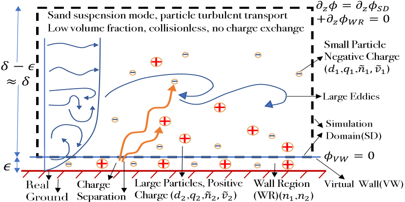
Figure 1: Schematic of the simulation domain (SD) . The atmospheric boundary layer height $\delta$ is modeled as a turbulent half-channel flow with streamwise and spanwise periodic conditions. The lower boundary of SD is modeled as a virtual wall (VW) at height $\epsilon\!\ll\!\delta$.

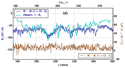
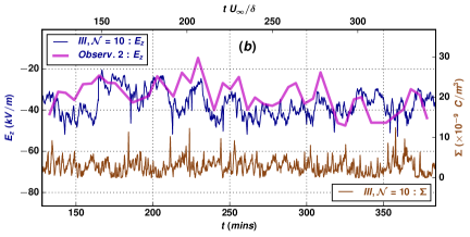
Figure 2: Time history of the simulated instantaneous wall-normal electric field (${E}_{z}$) at the mid-span mid-stream grid location (blue) along with the charge density variation (brown) at (a)14.2$m$, Case III-B and (b)35$m$, Case III where ${\mathcal{N}}=N_{w}/N_{1}$. Superimposed on the simulations are in-situ measurements by Zhang et al. Zhang et al. (2004) (Observ. 1) and Zhang et al. Zhang et al. (2018) (Observ. 2).

Computational setup and boundary conditions.- The above coupled set of equations governing the turbulent fluid flow with a suspension of charged sand particles is solved wherein the atmospheric boundary layer is modeled as a turbulent half-channel flow Calaf et al. (2010). The physical setup of the computational domain is depicted schematically in Fig. 1. The lower computational boundary is not at ground level but at an elevated height (denoted as $\epsilon$) into the log-layer of the channel flow – this is akin to the wall-modeled LES approach of Chung & Pullin Chung and Pullin (2009). We use periodic boundary conditions in the streamwise and spanwise direction for both the fluid and solid phases. At the virtual wall (VW), the wall model leads to a dynamic Dirichlet boundary condition for the fluid velocity Chung and Pullin (2009). At the ground level, sand particles collide with each other, exchange charge and get entrained into the flow. The physics of such a charge exchange and lift-off process is complex. Here, we assume that the charge exchange process takes place below the virtual wall. One approach is to parameterize this phenomenon as a flux boundary condition of charged sand particles into the flow, which is proportional to the number density, and dependent on many factors like soil humidity, ground temperatureas well as other wind erosion factors, and not just atmospheric flow Reynolds number. An alternative, simpler, approach is to specify a Dirichlet boundary condition for the particle number density distribution ($N_{w}$) at the virtual wall, i.e., an ${\mathcal{S}}$-vector of number density values is specified at the virtual wall. For the electrostatic potential we use a zero wall-normal gradient (Neumann BC) at the top ($\partial_{z}\phi_{SD}\!\!=\!0$), along with the Dirichlet BC (${\phi}_{VW}\!\!=\!0$) at the virtual wall. In order to maintain charge neutrality in the total domain (simulation domain (SD) plus the wall region (WR) ), the excess charge density in the simulation (SD) is distributed equally but with an opposite sign in the region below the virtual wall.
Numerical Methodology.- The description of the gas phase follows an earlier work Rahman and Samtaney (2017) on LES of incompressible turbulent flows (Eq. 1). The simulations employ the stretched spiral-vortex SGS model along with a wall model that uses an inner-scaling ansatz to derive an ODE for a virtual-wall velocity. The numerical solver is based on a fractional-step method with an energy-conserving fourth-order finite-difference scheme on a staggered mesh Rahman and Samtaney (2017). The dispersed solid phase (Eq. 3,2) is computed using the Eulerian approach of Direct Quadrature Method of Moments (DQMOM) Desjardins et al. (2008). The dynamic electrical interactions between charged particles are accounted for in the form of Gauss law (Eq. The generation and sustenance of electric fields in sandstorms), which is solved using the multigrid technique. The solution to the Poisson equation governing the electrostatic potential takes into account the charge distribution below the virtual wall. The numerical code has been extensively tested and validated Rahman et al. (2016).
Simulation Cases.- For all the simulation cases reported here, we fix the free stream velocity of $U_{\infty}\!\!\!=\!\!\!15$m/s and a boundary layer of size $\delta\!\!=\!\!\!1000m$ (this corresponds to a Reynolds number based on boundary layer thickness to be $Re_{\delta}\!\!=\!\!10^{9}\!$, corresponding to a kinematic viscosity of air of $1.5\!\!\times\!\!10^{-5\!}m^{2}\!/\!s$). We sample the particle number density distribution function at two points ($\!\mathcal{S}\!\!=\!\!2$), i.e., the sand phase is comprised of two sizes ($d_{1}\!\!\!=\!\!200\mu m,d_{2}\!\!\!=\!\!500\mu m)$ of mass density $2650Kg\!/\!m^{3\!}$. The representative (ideal) electric charge of the species of each size is $Q_{1}\!\!\!\equiv\!\!(q_{1},q_{2})\!\!=\!\!(-4\!\times\!10^{-15}C,2.24\!\times\!10^{-15}C)$. A typical concentration Liu and Dong (2004) at the bottom of suspension (top of saltation, O(1m)) are $N_{1}\!\!\!=\!\!(\!{n}_{1\!},\!{n}_{2\!})\!\!=\!\!(2\!\times\!10^{7\!}m^{\!-3}\!,\!3.4\!\times\!10^{6\!}m^{\!-3\!})$. Four cases are considered in which the boundary conditions at the virtual wall $N_{w}$ is varied from $N_{1}$ (corresponding to a weak storm) to $40N_{1}$ (corresponding to a very strong sandstorm). These cases are labeled as: Case I ($N_{w}\!\!\!=\!\!\!N_{1}$, “weak”), Case II ($N_{w}\!\!=\!\!4N_{1}$, “moderate”), Case III ($N_{w}\!\!\!=\!\!\!10N_{1}$, “strong”),Case IV ($N_{w}\!\!=\!\!40N_{1}$, “very strong”). Case III-B ($N_{w}\!\!=\!\!12N_{1}$, close to Case III) is included because it corresponds to field measurements of strong sandstorms. Other parameters used in simulations are as follows. The fluid simulation domain is $x\!\!=\!\!32\delta$, $y\!\!=\!\!8\delta$, and $z\!\!=\!\!\delta$, with $768$, $192$ and $96$ grid points in the $x$, $y$ and $z$ directions, respectively. The solid simulation domain in the wall-normal direction was truncated at $z\!\!=\!\!0.5\delta$ to capture the near ground particle dynamics. The characteristic grid spacings in viscous wall units are $\Delta x^{+}\!\!\!=\!\!16\!\times\!10^{5}$, $\Delta y^{+}\!\!\!=\!\!16\!\times\!\!10^{5}$ and $\Delta z^{+}\!\!\!=\!\xi^{+}\!\!\!=\!4\!\times\!\!10^{5}$. The virtual wall height $\epsilon$ in terms of viscous wall units is at $z^{+}\!\!\!=\!\!1.5\!\!\times\!\!10^{4}$.

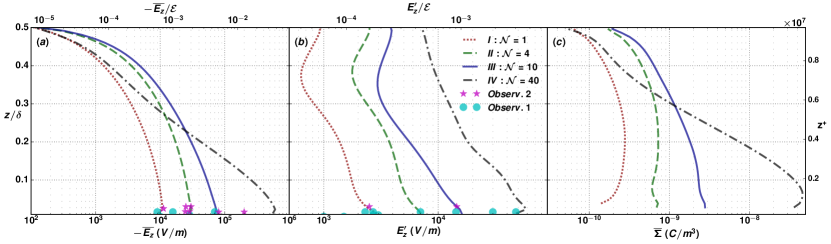
Figure 3: Altitude variation of the wall-normal electric field (a) mean (time and streamwise/spanwise averaged) $\bar{E}_{z}$, (b) RMS of fluctuations ${E}_{z}^{\prime}$, and (c) mean charge density, where $\mathcal{E}={\delta\ {{\mathbf{\mathrm{M}}}(n_{{}_{1}}|q_{{}_{1}}|,n_{{}_{2}}|q_{{}_{2}}|)}}{/\varepsilon}$ is a reference electric field value corresponding to Case I ($M(a,b)=$mean of $a$ and $b$). The symbols are mean and RMS values synthesized from various sandstorm measurements of Zhang et al. Zhang et al. (2004) (circles) and Zhang et al. Zhang et al. (2018) (stars).

Results.- Before we present results of the turbulence simulations, we remark that we performed simulations for the fluid laminar regime comprising of a Poiseuille velocity profile. These laminar simulations yielded RMS electric field values smaller by orders of magnitude than those from turbulent simulations, further lending credence to our hypothesis.
Comparison with Field Observations.- The time variation of ${E}_{z}$ is plotted in Fig. 2 wherein we superimpose our simulation results with field observations Zhang et al. (2004, 2018). Since the time origin is somewhat arbitrary we align the minimum of ${E}_{z}$ (Fig. 2(a)) and the pattern variation of ${E}_{z}$ (Fig. 2(b)) between the observations and simulations. The overall average magnitude of ${E}_{z}$ from simulations compares well with the field observations although it is evident that the simulations also depict higher frequencies in the variation of ${E}_{z}$ compared with the observations (which may be limited due to instrumentation).
Varying sandstorm strength.- Cases I–IV are chosen to progressively increase in strength from weak to very strong sandstorms. We compute the flow until it is statistically steady following which the vertical component of the electric field ${E}_{z}$ is time-averaged over the horizontal plane $\overline{{E}}_{z}$ and the RMS  (root-mean-square) of ${E}_{z}^{\prime}$. For all four cases, the altitude variation of $\overline{{E}}_{z}$ and ${E}_{z}^{\prime}$, and the mean charge density $\overline{\Sigma}$ are plotted in Fig. 3. The mean net electric field Fig. 4 (a) of the cases decreases with height because of the decrease in the mean profile of charge density. As the boundary number density ($N_{w}$) increases, the mean and fluctuation magnitudes of electric field also increases. For each case, the magnitude of mean and RMS values decrease with altitude. The mean magnitude of the horizontal components of the electric field is negligible because of streamwise and spanwise periodic boundary conditions, but the RMS values are of the same order of magnitude as the vertical component. For the sandstorm case III, we note the instantaneous maximum ${|{{\bf E}}|\!\!=\!\!200kV\!/\!m}$ and range of ${{E}}_{z}\in(-70,\!130)kV\!\!/\!m$ in the domain. For cases III, III-B and IV, the maximum magnitude of horizontal electric field exceeds 100$kV\!/\!m$, which is also observed in the field Jackson and Farrell (2006). For the weak sandstorm case (Case I) the near wall average electric field ($\overline{{E}}_{z}$) are close to the observed electric field, ($\overline{{E}}_{z}\!\!\approx\!\!-10KV\!/m)$ Zhang et al. (2018), while for Case II (moderate) $\overline{{E}}_{z}\!\!\approx\!\!-30KV\!/m$ and Case III (strong sandstorm) observations $\overline{{E}}_{z}\!\!\approx\!\!-80KV/m$, agree with field measurements Zhang et al. (2004, 2018). The RMS fluctuation of the near wall vertical electric field for the case II, Fig. 3(b), is close to the $7kV\!\!/\!m$ observed in the field Bo and Zheng (2013). The instantaneous electric fields are in the same or opposite direction of the Earth’s background electric field. The instantaneous fluctuations at some locations are sufficiently high to cause a reversal in the direction of the vertical electric field component. Such a change in the direction of the electric field has been observed in the field Zhang et al. (2018), and similarly observed in the saltation layer Schmidt et al. (1998). An incremental change in particle concentration boundary conditions tends to increase the electric field levels in the sandstorms. The mean charge density plotted in Fig. 3 (c) shows that its magnitude is at its maximum close to the wall. Although not shown, we note that the largest charge density fluctuation also occurs in the vicinity of the wall and is well-correlated with the turbulent intensity of the flow.

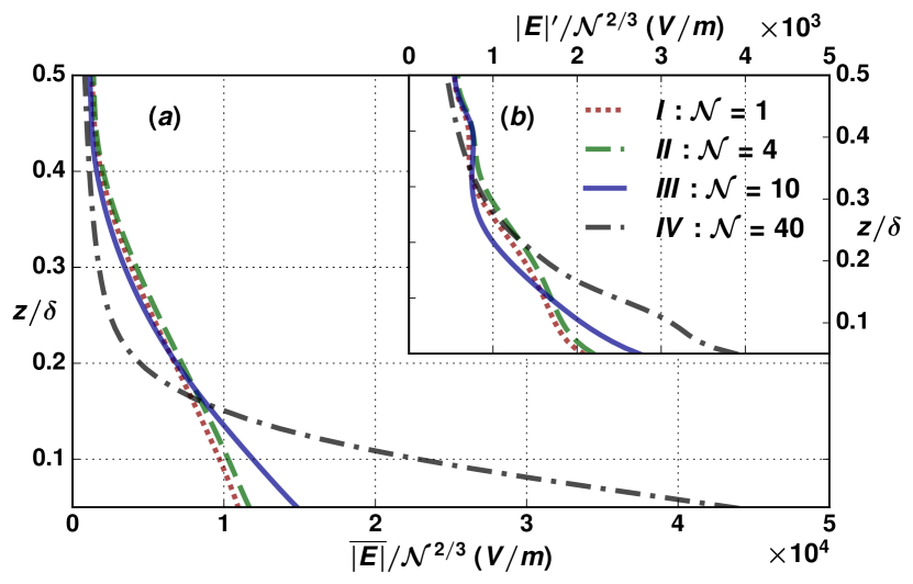
Figure 4: Altitude variation of the (compensated) net electric field magnitudes of (a) mean $\overline{|{{\bf E}}|}$ and (b) RMS fluctuations $|{{\bf E}}|^{\prime}$ scaled by ${\mathcal{N}}^{\frac{2}{3}}$.

Self-similarity.- In the simulations considered above, the fluid turbulence is identical in all cases because of the one-way coupling between the fluid and the solid phases. The differences in the charge density stem from the differences in the flux of the sand particles into the turbulent flow. The fundamental electrostatic charge interaction scales as $E\!\!\propto\!\!q/r^{2}$. Combining this with the fact that in dilute particle flow, the average inter-particle distance ($\!\propto\!\!{\tilde{n}_{s}}^{\!-1\!/3\!}$) for a low volume fraction of particles leads to the the $2\!/\!3$ scaling power law for the electric field, i.e., $E\!\!\propto\!\!1\!/\!r^{2}\!\!\propto\!{\mathcal{N}}^{2\!/\!3}$. The compensated electric field magnitude (normalized by ${\mathcal{N}}^{2\!/\!3\!}$) of both the mean and RMS as a function of normalized distance are plotted in Fig. 4.
Summary.- We have presented a framework to simulate a sandstorm modeled as the flow of charged sand particles in a turbulent flow of a statistically steady atmospheric boundary layer. The computed values match those observed in sandstorms. A further increase in the concentration of electrically charged particles can reach the breakdown field in air, and therefore can trigger lightning (not modeled here). Our analysis demonstrates that the charge and concentration of sand particles are crucially responsible for the dynamics in sandstorms. The electric fields produced in sandstorm conditions can be in the same or opposite direction to Earth’s normal electric field and decrease with altitude. We propose a simple scaling $\overline{|{{{\bf E}}}|},\!|{{\bf E}}|^{\prime}\!\!\propto\!{\mathcal{N}}^{2\!/\!3}$ that holds well for weak-to-moderate strength sandstorms. We posit that the level and frequency of occurrence of atmospheric turbulence will increaseStorer et al. (2017) in the coming decades with the impact of climate change, making such studies more relevant. Even though this work concentrates on earthbound dust suspension, our simulation framework can also be useful for modeling severe Martian sandstorms with suitable parameters.
Authors acknowledge the support of KAUST under awards URF/1/1704-01-01 & BAS/1/1/1349-01-1. Cray XC40 Shaheen II at KAUST was used for simulations.

References

- Baddeley (1860) P. F. H. Baddeley, Whirlwinds and Dust-storms of India (Bell & Daldy, 1860).
- Zhang et al. (2004) H. F. Zhang, T. Wang, J. J. Qu, and M. H. Yan, Chinese Journal of Geophysics 47, 53 (2004).
- Keith (1944) B. A. Keith, Transactions of the Kansas Academy of Science (1903-) 47, 95 (1944).
- Eden and Vonnegut (1973) H. F. Eden and B. Vonnegut, Science 180, 962 (1973).
- Jackson and Farrell (2006) T. L. Jackson and W. M. Farrell, IEEE Transactions on Geoscience and remote sensing 44, 2942 (2006).
- Pähtz et al. (2010) T. Pähtz, H. J. Herrmann, and T. Shinbrot, Nature Physics 6, 364 (2010).
- Kanagy and Mann (1994) S. Kanagy and C. J. Mann, Earth-Science Reviews 36, 181 (1994).
- Zheng et al. (2003) X. J. Zheng, N. Huang, and Y.-H. Zhou, Jour. of Geophys. Research: Atmospheres (1984–2012) 108 (2003).
- Kok and Renno (2008) J. F. Kok and N. O. Renno, Phys. Rev. Lett. 100 (2008).
- Zhang et al. (2010) Y. Zhang, J. Yang, D. Liu, X. Wei, and L. Yu, Particuology 8, 325 (2010).
- Balachandar and Eaton (2010) S. Balachandar and J. K. Eaton, Annual Review of Fluid Mechanics 42, 111 (2010).
- Zhang et al. (2018) X. Zhang, D. Li, and T.-L. Bo, Granular Matter 20 (2018), 10.1007/s10035-018-0801-6.
- Calaf et al. (2010) M. Calaf, C. Meneveau, and J. Meyers, Physics of fluids 22, 015110 (2010).
- Chung and Pullin (2009) D. Chung and D. I. Pullin, Jour. of Fluid Mech. (2009).
- Rahman and Samtaney (2017) M. M. Rahman and R. Samtaney, in 55th AIAA Aerospace Sciences Meeting (2017) p. 0981.
- Desjardins et al. (2008) O. Desjardins, R. O. Fox, and P. Villedieu, Journal of Computational Physics 227, 2514 (2008).
- Rahman et al. (2016) M. Rahman, W. Cheng, R. Samtaney, and J. Urzay, in Proceedings of the Summer Program (2016) p. 45.
- Liu and Dong (2004) X. Liu and Z. Dong, Geomorphology 60, 371 (2004).
- Bo and Zheng (2013) T.-L. Bo and X.-J. Zheng, Aeolian Research 8, 39 (2013).
- Schmidt et al. (1998) D. S. Schmidt, R. A. Schmidt, and J. D. Dent, Jour. of Geophys. Resear.: Atmospheres (1984–2012) 103 (1998).
- Storer et al. (2017) L. N. Storer, P. D. Williams, and M. M. Joshi, Geophysical Research Letters 44, 9976 (2017).