Constraining galactic structures of mirror dark matter

Abstract

The simplest model of mirror sector dark matter maintains exact mirror symmetry, but has a baryon abundance $\Omega_{b^{\prime}}=\beta\Omega_{b}$ and a suppressed temperature $T^{\prime}=xT$ in the mirror sector; hence it depends only on two parameters, $\beta,x$. For sufficiently small $x$, early cosmological observables may not constrain mirror baryons from constituting all of the dark matter despite their strong self-interactions, depending on the unknown details of structure formation in the hidden sector. Here we close this loophole by simulating mirror structure formation, mapping out the allowed regions of parameter space using cosmological and astronomical data. We find that the Milky Way disk surface density and bulge mass constrain $\Omega_{b^{\prime}}\lesssim 0.3\Omega_{b}$ at the highest $T^{\prime}$ allowed by BBN and CMB ($T^{\prime}=0.5T$), or $\Omega_{b^{\prime}}\lesssim 0.8\Omega_{b}$ at lower values of $T^{\prime}$. We also briefly discuss the realization of the necessary temperature asymmetry between the SM and the mirror sector in our model with unbroken mirror symmetry.

I Introduction

The idea of a mirror copy of the standard model is the earliest example of the now-popular paradigm of hidden dark sectors Kobzarev:1966qya ; Okun:2006eb . The model has a number of appealing features, the most obvious being that a CP-like transformation is restored as a symmetry of nature, and dark matter candidates (mirror baryons) are provided Hodges:1993yb , including a resolution of the cusp-core problem Mohapatra:2000qx . Twin Higgs models are one specific realization of mirror matter set to solve the little hierarchy problem Chacko:2005pe . More recently a subdominant mirror sector ( SM ) has been suggested for stimulating the early growth of supermassive black holes DAmico:2017lqj ; Latif:2018kqv and neutron – mirror neutron oscillations have been proposed as a solution to the neutron lifetime puzzle Berezhiani:2018eds . A detailed review of the general model is available in ref. Foot:2014mia .

A priori, it seems possible that mirror baryons could constitute all of the dark matter (DM), even though dark atoms have an interaction cross section far exceeding the bounds from the Bullet Cluster Markevitch:2003at ; Randall:2007ph . If the mirror baryons are present primarily in collapsed structures rather than gaseous atoms or molecules, their self-interaction cross section would be sufficiently small, just like ordinary stars are effectively collisionless. Moreover the strong constraints on atomic Cyr-Racine:2013fsa or mirror Ciarcelluti:2010zz dark matter from dark acoustic oscillations can be evaded if the SM  temperature $T^{\prime}$ is sufficiently low ($\lesssim 0.3\,T$) compared to that of visible photons.

A major goal of the present work is to determine what fraction of the total DM density could be in mirror particles, by studying structure formation in the SM . Assuming that mirror symmetry is unbroken, we can do this exhaustively, since there are only two parameters to vary: the relative abundance of mirror versus visible baryons $\beta=\Omega_{b^{\prime}}/\Omega_{b}$, and the temperature ratio $x=T^{\prime}/T$. An additional particle that is noninteracting and uncharged under the mirror symmetry is taken to comprise the remainder of the DM, if necessary. Throughout this work, primes will distinguish elements of the SM  analogous to the visible ones. We assume that the possible portal interactions between the two sectors (Higgs mixing $h^{2}h^{\prime 2}$ and gauge kinetic mixing $F^{\mu\nu}F^{\prime}_{\mu\nu}$) are negligible, since these would cause $x\to 1$ if they were sufficiently strong.

We adopt a methodology similar to ref. Ghalsasi:2017jna , which studied structure formation in a simplified atomic dark matter model. Namely we use the extended Press-Schechter formalism Press:1973iz ; Bond:1990iw ; Lacey:1993iv and the semi-analytical model GALFORM Cole:2000ex to simulate the merger history of DM halos and study the formation of dark galactic structures. Unlike the dark atomic model, mirror DM contains nuclear reactions which allow mirror helium formation and stellar feedback to alter the evolution of DM structures. We consider the effects of these extra features in the hidden sector quantitatively.

In order to predict structure formation, one must first understand the early-universe cosmology of the model, leading to the primordial mirror abundances and ionization fractions. As well, constraints on additional radiation degrees of freedom are imposed by the cosmic microwave background (CMB) and big-bang nucleosynthesis (BBN). This is worked out in sect. II. These inputs allow us to simulate structure formation in the SM  using the semi-analytical galaxy formation model GALFORM, which we describe in sect. III. In sect. IV, we present our results and the constraints on the parameters $x,\beta$ coming from astronomical observations. In sect. V we discuss early cosmological scenarios that could produce values of $x,\beta$ consistent with our constraints without explicitly breaking the mirror symmetry. Conclusions are given in sect. VI.

Throughout this paper we will use the following cosmological parameters Tanabashi:2018oca : $h=0.678$, $T_{0}=2.7255$ K, $\Omega_{m}=0.308$, $\Omega_{b}=0.0484$, $\Omega_{\Lambda}=0.692$, $n_{s}=0.968$ and $\sigma_{8}=0.815$. Although most of these values were derived assuming a $\Lambda$CDM cosmology, our conclusions would not change significantly if we used slightly different parameters.

II Cosmology of the mirror sector

We assume that a fraction of dark matter resides in a hidden sector whose gauge group $G^{\prime}$ is a copy of the Standard Model (SM) gauge group $G=SU(3)\times SU(2)\times U(1)$. This model possesses a discrete mirror symmetry $P_{G\leftrightarrow G^{\prime}}$ that interchanges the fields of the ordinary, observable sector with their mirror counterparts. If $P_{G\leftrightarrow G^{\prime}}$ is unbroken as we assume, then the microphysics of each sector is identical. In particular, mirror matter comprises the same chemical and nuclear species as ordinary matter and all their processes have the same rates. Although $P_{G\leftrightarrow G^{\prime}}$ does not forbid the two renomalizable gauge kinetic mixing and Higgs portal interactions between the two sectors, we assume that the portal couplings are sufficiently small as to have negligible impact on early cosmology and structure formation. Hence SM particles interact with their mirror counterparts only gravitationally.

Eventually we will confirm that mirror baryons cannot comprise all of the DM, necessitating an additional component in the form of standard cold, collisionless dark matter (CDM) that is assumed to interact with the other sectors only gravitationally. The total matter density in the universe is then $\Omega_{m}=\Omega_{c}+\Omega_{b}+\Omega_{b^{\prime}}$, where $\Omega_{c}$ is the CDM fraction and $\Omega_{b}$ ($\Omega_{b^{\prime}}$) is the ordinary (mirror) baryon relic density, in units of the critical density.

Because of the mirror symmetry, $\Omega_{b}$ and $\Omega_{b^{\prime}}$ would likely originate from the same mechanism; nevertheless $\Omega_{b^{\prime}}$ can be different from $\Omega_{b}$ if the two sectors have different initial temperatures 1985Natur.314..415K ; Berezhiani:2000gw . We accordingly take $\beta\equiv\Omega_{b^{\prime}}/\Omega_{b}$ as a second free parameter, in addition to the temperature ratio $x\equiv T^{\prime}/T$. In fact $T^{\prime}/T$ is time-dependent during early cosmology, for example through $e\bar{e}$ and $e^{\prime}\bar{e}^{\prime}$ annihilations occurring at different redshifts, which produces a relative difference of entropy in the photon backgrounds during some period. But it becomes constant at the late times relevant for structure formation, hence we define $x$ to be the asymptotic value. This remains true even in the presence of portal interactions between the two sectors, as long as they are weak enough to freeze out before the onset of structure formation.

II.1 Effective radiation species

BBN and the CMB constrain the expansion rate of the universe and thereby the total radiative energy density. This is conventionally expressed as a limit on the number of additional effective neutrino species $\Delta N_{\textrm{eff}}=N_{\textrm{eff}}-3.046$. The contribution to $\Delta N_{\textrm{eff}}$ from the mirror photons and neutrinos follows from Berezhiani:2000gw

$$\Delta\rho_{\textrm{rad}}=\frac{7}{8}\left(\frac{T_{\nu}}{T}\right)^{4}\Delta N_{\textrm{eff}}\ \rho_{\gamma}=\frac{\pi^{2}}{30}g_{*}^{\prime}(T^{\prime})\ T^{\prime 4},$$ (1)

where $\rho_{\gamma}$ is the energy density of ordinary photons and $g_{*}^{\prime}(T^{\prime})$ is the effective number of relativistic degrees of freedom in the SM . Using $\rho_{\gamma}=(2\pi^{2}/30)T^{4}$ and $T_{\nu}/T=(4/11)^{1/3}$ today we find that

$$\Delta N_{\textrm{eff}}=\frac{4}{7}\left(\frac{11}{4}\right)^{4/3}g_{*}^{\prime}(T^{\prime})\ x^{4}.$$ (2)

The most recent data from the Planck Collaboration indicates that at the epoch of recombination $N_{\textrm{eff}}=2.99^{+0.34}_{-0.33}$ with 95 % confidence Aghanim:2018eyx , which gives the 3$\sigma$ limit $\Delta N_{\textrm{eff}}[\textrm{CMB}]<0.45$. At this temperature only photons and neutrinos are relativistic so $g_{*}^{\prime}(T^{\prime})=3.38$, leading to the bound

$$x\lesssim 0.5.\text{\leavevmode\nobreak\ \leavevmode\nobreak\ \leavevmode\nobreak\ (CMB)}$$ (3)

BBN sets a similar limit on $x$, even using the more stringent bound on the effective neutrino species $\Delta N_{\textrm{eff}}[\textrm{BBN}]\lesssim 0.3$ Cyburt:2015mya ; Hufnagel:2017dgo . This is because, although neutrinos are decoupled from photons at the BBN temperature, nominally $T_{\scriptscriptstyle BBN}\sim 1\,$MeV, $e\bar{e}$ pairs haven’t annihilated yet, such that $T_{\nu}\simeq T_{\gamma}$ and the factor of $(4/11)^{4/3}$ is removed from from eq. (2). Moreover for $x=0.5$, $g_{*}^{\prime}(T^{\prime})=g_{*}(0.5\,T_{\scriptscriptstyle BBN})\simeq 10$, leading to the bound $x<0.48$, which is essentially the same as the CMB constraint (3). Using lower values of $g_{*}^{\prime}(T^{\prime})$ would make this limit less stringent.

II.2 Mirror nucleosynthesis

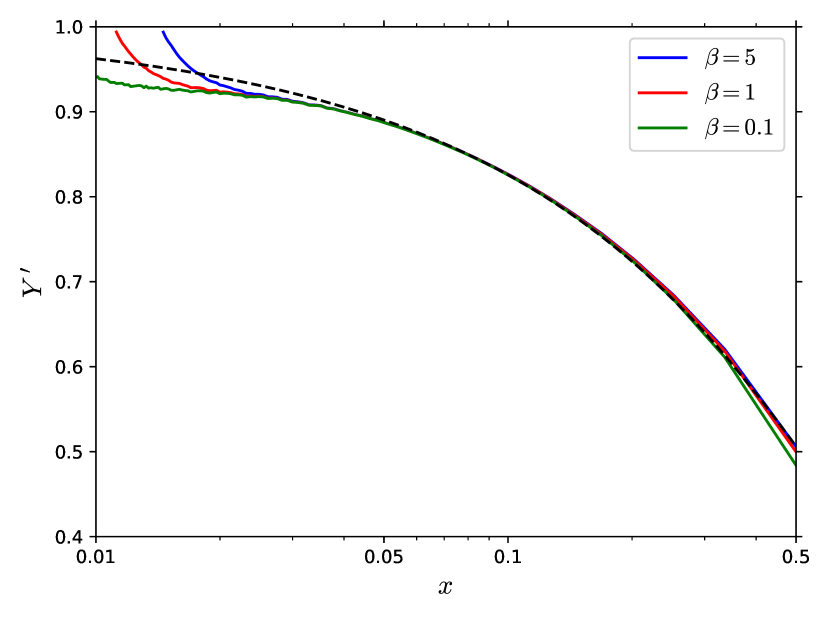
Figure 1: Mirror ⁴He relic abundances. The solid curves were computed numerically using AlterBBN— and the dashed line shows the approximate formula of eq. (4).

The upper limit on $x$ leads to an important feature of mirror matter: it has a large helium abundance, stemming from the early freeze-out of $n^{\prime}\leftrightarrow p^{\prime}$ equilibrium. This implies a higher relic neutron abundance and consequently more efficient deuterium and helium production in the SM . Early freeze-out of mirror interactions is a general consequence of the temperature hierarchy $T^{\prime}<T$, which causes a cosmological event (tied to some temperature scale), occurring at redshift $z$ in the visible sector, to transpire at higher redshift $z^{\prime}\simeq-1+(1+z)/x$ in the SM . Since the universe was expanding more rapidly at redshift $z^{\prime}$ than at $z$, the freeze-out of mirror processes will generally occur even earlier than this estimated $z^{\prime}$.

An approximate formula for the relic ⁴He^′ mass fraction was derived in ref. Berezhiani:2000gw ,

$$Y^{\prime}\simeq\frac{2\exp{\left[-t_{N}/\tau(1+x^{-4})^{1/2}\right]}}{1+\exp{\left[\Delta m/T_{W}(1+x^{-4})^{1/6}\right]}},$$ (4)

where $t_{N}\sim 200\,$s is the age of the universe at the “deuterium bottleneck”, $\tau=886.7\,$ s is the neutron lifetime, $T_{W}\simeq 0.8\,$ MeV is the $n^{\prime}\leftrightarrow p^{\prime}$ freeze-out temperature, and $\Delta m=1.29\,$ MeV is the neutron-proton mass difference. This relation is plotted in fig. 1.

The approximation (4) neglects possible dependence on $\beta$. A more accurate treatment of BBN is required to determine how the density of mirror baryons affects the freeze-out temperature of light nuclei and their relic abundances. We used the code AlterBBN Arbey:2011nf ; Arbey:2018zfh to numerically compute the residual (mirror) ⁴He^′ mass fraction for different values of $\beta$, modifying parameters of the code to match the conditions of the SM . Namely the current CMB temperature, the baryon density and the baryon-to-photon ratio were replaced by $T_{0}\rightarrow T_{0}/x$, $\Omega_{b}\rightarrow\beta\Omega_{b}$ and $\eta_{b}\rightarrow\eta_{b}\beta/x^{3}$. Visible sector photons and neutrinos were incorporated as additional effective neutrino species. Rewriting eqs. (1,2) from the perspective of the mirror world yields $\Delta N_{\textrm{eff}}^{\prime}\simeq 7.44/x^{4}$ today.

The results of our numerical calculations are also plotted in fig. 1 for three benchmark values of $\beta$. Eq. (4) agrees with the numerical calculations within a few percent, which is sufficient for our purposes in the following analysis. The striking domination of ⁴He^′ in the SM , in the limit when $x\rightarrow 0$ for fixed $\beta$, is contrary to statements made in refs. DAmico:2017lqj ; Latif:2018kqv . One sees that for any value of $\beta$, the ⁴He^′ fraction reaches $1$ as $x$ decreases to some critical value. The AlterBBN code is not suited to handle the situation where the mirror hydrogen (H^′) abundance vanishes since H^′ is used as a reference to normalize other abundances. Thus we cannot keep track of very small H^′ densities. Moreover the age of the universe at the formation of mirror deuterium scales roughly as $t_{N}\sim x^{2}$; hence for small values of $x$ nucleosynthesis occurs in a fraction of a second and the Boltzmann equations for each species become too stiff for AlterBBN to maintain a high accuracy. But this has no impact on our main results since both eq. (4) and our numerical analysis agree that the ⁴He^′ abundance is limited to $0.9<Y^{\prime}<1$ for small values of $x$, with little phenomenological variation within this range.

The ⁴He^′ abundance determines a number of other quantities that will be useful in the subsequent analysis. Let $X_{i}\equiv n_{i}/n_{\mathrm{H}}$ be the relative abundance of a given chemical species, conventionally normalized to the H^′ density. The helium-hydrogen number ratio is

$$X_{\mathrm{He}}\equiv\frac{n_{\mathrm{He}}}{n_{\mathrm{H}}}=\frac{m_{p}}{m_{\mathrm{He}}}\frac{Y^{\prime}}{1-Y^{\prime}}\simeq\frac{1}{4}\frac{Y^{\prime}}{1-Y^{\prime}},$$ (5)

where $m_{p}$ is the proton mass. Furthermore the helium number fraction (distinct from the mass fraction $Y^{\prime}=m_{\mathrm{He}}n_{\mathrm{He}}/(m_{\mathrm{He}}n_{\mathrm{He}}+m_{\mathrm{H}}n_{\mathrm{H}})$) is

$$\qquad\qquad f_{\mathrm{He}}\equiv\frac{n_{\mathrm{He}}}{n_{N}}=\frac{1}{1+1/X_{\mathrm{He}}}\simeq\frac{Y^{\prime}}{4-3Y^{\prime}},\qquad\$$ (6)

with $n_{N}=n_{\mathrm{H}}+n_{\mathrm{He}}$ denoting the number density of nuclei. The mean mass per nucleus is

$$\overline{m_{N}}=\left(\frac{1-Y^{\prime}}{m_{p}}+\frac{Y^{\prime}}{m_{\mathrm{He}}}\right)^{-1}\simeq\frac{m_{p}}{1-\frac{3}{4}Y^{\prime}}.$$ (7)

By virtue of the approximation made in eq. (4), the expressions (5-7) are independent of $\beta$. Lastly, the background number density of nuclei at any redshift follows from

$$n_{N}=\frac{3H_{0}^{2}\Omega_{b}}{8\pi G}\frac{\beta}{\overline{m_{N}}}(1+z)^{3}\ ,$$ (8)

implying that $n_{\mathrm{H}}=(1-f_{\mathrm{He}})n_{N}$ and $n_{\mathrm{He}}=f_{\mathrm{He}}n_{N}$.

II.3 Recombination

Due to its lower temperature, recombination in the SM  occurs at the higher redshift $z_{\mathrm{rec}}^{\prime}\simeq 1100/x$. With its large fraction of mirror He, that has a higher binding energy than H, this leads to more efficient recombination and a lower residual free electron density. Primordial gas clouds require free electrons to cool and collapse into compact structures. Therefore the small relic ionization fraction has a direct impact on the formation of the first mirror stars.

Recombination proceeds through three major steps, which are the respective formation of He⁺, He⁰ and H⁰. The latter is prevalent in the SM, but recombination of He is more important in the SM  because of its high abundance. We adopt the effective three-level calculation presented in ref. Seager:1999bc which was also used in ref. DAmico:2017lqj .

Recombination of He⁺ in the SM occurred around $z\simeq 6000$ ($kT\sim 1.4\,\mathrm{eV}$), at a sufficiently high density for the ionized species to closely track their thermodynamic equilibrium abundances, in accordance with the Saha equation. Since recombination occurs even earlier in the SM , this is also true for mirror He⁺. Its Saha equation is

$$\frac{\left(X_{e}-1-X_{\mathrm{He}}\right)X_{e}}{1+2X_{\mathrm{He}}-X_{e}}=\frac{\left(2\pi m_{e}kT^{\prime}\right)^{3/2}}{h^{3}n_{\mathrm{H}}}e^{-\chi_{\mathrm{He^{+}}}/kT^{\prime}},$$ (9)

where $\chi_{\mathrm{He^{+}}}=54.4\$eV is the He⁺ ionization energy, $T^{\prime}=xT_{0}(1+z)$ is the mirror photon temperature and the free electron ratio is $X_{e}=X_{\mathrm{H^{+}}}+X_{\mathrm{He^{+}}}+2X_{\mathrm{He^{++}}}$ from matter neutrality. For $kT^{\prime}\sim 1.4\,\mathrm{eV}$, the exponential in eq. (9) is negligible, giving $X_{e}=1+X_{\mathrm{He}}$. Eliminating $X_{e}$ and using the fact that $X_{\mathrm{H^{+}}}\simeq 1$ and $X_{\mathrm{He^{0}}}\simeq 0$ (there is essentially no neutral H or He until $T^{\prime}$ falls below $\sim 10\leavevmode\nobreak\ \%$ of the $n=2$ ionization energies of H or He, i.e. until $kT^{\prime}\lesssim 0.4\,$eV), this implies $X_{\mathrm{He^{++}}}\simeq 0$: we can neglect any residual He⁺⁺ fraction, and both H and He are singly ionized.

At later times, the evolution of the ionized states follows the network Seager:1999bc

$$\frac{dX_{\mathrm{H^{+}}}}{dz} = \frac{\left(X_{e}X_{\mathrm{H^{+}}}n_{\mathrm{H}}\alpha_{\mathrm{H}}-\beta_{\mathrm{H}}(1-X_{\mathrm{H^{+}}})e^{-h\nu_{\mathrm{H}}/kT_{M}^{\prime}}\right)\left(1+K_{\mathrm{H}}\Lambda_{\mathrm{H}}n_{\mathrm{H}}(1-X_{\mathrm{H^{+}}})\right)}{H(z)(1+z)(1+K_{\mathrm{H}}(\Lambda_{\mathrm{H}}+\beta_{\mathrm{H}})n_{\mathrm{H}}(1-X_{\mathrm{H^{+}}}))},$$ (10)

$$\frac{dX_{\mathrm{He^{+}}}}{dz} = \frac{\left(X_{e}X_{\mathrm{He^{+}}}n_{\mathrm{H}}\alpha_{\mathrm{He^{0}}}-\beta_{\mathrm{He^{0}}}(X_{\mathrm{He}}-X_{\mathrm{He^{+}}})e^{-h\nu_{\mathrm{He}}/kT_{M}^{\prime}}\right)\left(1+K_{\mathrm{He^{0}}}\Lambda_{\mathrm{He}}n_{\mathrm{H}}(X_{\mathrm{He}}-X_{\mathrm{He^{+}}})e^{-h\tilde{\nu}_{\mathrm{He}}/kT_{M}^{\prime}}\right)}{H(z)(1+z)(1+K_{\mathrm{He^{0}}}(\Lambda_{\mathrm{He}}+\beta_{\mathrm{He^{0}}})n_{\mathrm{H}}(X_{\mathrm{He}}-X_{\mathrm{He^{+}}})e^{-h\tilde{\nu}_{\mathrm{He}}/kT_{M}^{\prime}})},$$ (11)

$$\frac{dT_{M}^{\prime}}{dz} = \frac{8\sigma_{T}a_{R}T^{\prime 4}}{3H(z)(1+z)m_{e}c}\left(\frac{X_{e}}{1+X_{\mathrm{He}}+X_{e}}\right)(T_{M}^{\prime}-T^{\prime})+\frac{2T_{M}^{\prime}}{(1+z)}.$$ (12)

that describes the the evolution of the He⁺ and H⁺ fractions, and the matter temperature $T_{M}^{\prime}$, which at low redshifts is below the radiation temperature $T^{\prime}$. The various parameters are specified in appendix A.

We used Recfast++ Seager:1999bc ; Chluba:2010ca ; RubinoMartin:2009ry ; Chluba:2010fy ; Switzer:2007sn ; Grin:2009ik ; 2010PhRvD..82f3521A to solve the system (10-12), making the same modifications as for AlterBBN, with the He mass fraction given by eq. (4). It was assumed that the species were initially singly ionized ($X_{\mathrm{H^{+}}}=1$, $X_{\mathrm{He^{+}}}=X_{\mathrm{He}}$) and that matter was strongly coupled to radiation ($T_{M}^{\prime}=T^{\prime}$). The initial redshift was taken to be sufficiently high to encompass the beginning of H⁰ and He⁰ recombination, and the system was evolved until $z=10$, the initial redshift of the subsequent structure formation analysis (see below). Fig. 2 shows the resulting evolution of the free electron fraction $f_{e}^{\prime}=n_{e}/n_{e,\mathrm{tot}}$ (where $n_{e,\mathrm{tot}}$ includes the electrons in the ground state of He⁺) during recombination for several values of $x$ (differentiated by color) and $\beta$ (differentiated by linestyle). The expected $x$-dependence of the redshift of recombination $z_{\rm rec}^{\prime}\sim 1100/x$ is evident, scaling inversely to the SM  temperature.

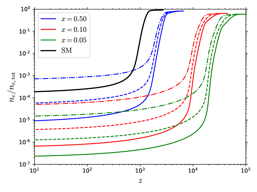
Figure 2: Evolution of the total ionization fraction during mirror recombination. The solid, dashed and dash-dotted curves represent $\beta=$ 5, 1 and 0.1, respectively. Also shown for comparison is recombination in the SM.

The most important feature for structure formation is the residual ionization fraction $f_{e}^{\prime}$ at low redshifts. As fig. 2 demonstrates, $f_{e}^{\prime}$ is typically much smaller in the SM  than in the SM ($f_{e}\sim 2\times 10^{-4}$). Only when $\beta\ll 1$ can $f_{e}^{\prime}$ reach higher values, because the low density reduces the number of ion-electron collisions and the overall efficiency of recombination. But in this case the total electron density is also suppressed by a factor of $\beta$, so the free electron density after recombination is always smaller in the SM . This can have important consequences for early structure formation, since without a significant ionization fraction mirror matter clouds may not cool and collapse to form structures like ordinary matter does.

Fig. 3 shows the $(x,\beta)$-dependence of the residual ionization fractions of H and He at $z=10$. For comparison, the SM values (at $x=1,\,\beta=1,\,Y=0.24$) are $n_{\mathrm{H^{+}}}/n_{\mathrm{H}}=2.2\times 10^{-4}$ and $n_{\mathrm{He^{+}}}/n_{\mathrm{He}}=1.2\times 10^{-12}$. Recombination of He is more efficient (blue regions) for high $\beta$, because a larger mirror matter density increases the collision rate between ions and free electrons. As $x$ decreases, the interval between the beginning of recombination ($z_{\mathrm{rec}}^{\prime}\simeq 1100/x$) and $z=10$ becomes longer, increasing the number of occasional ion-electron collisions following freeze-out. This and the slightly larger value of $n_{\mathrm{He}}$ explain the somewhat higher efficiency of He recombination at low $x$.

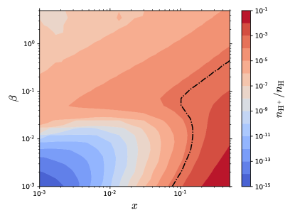
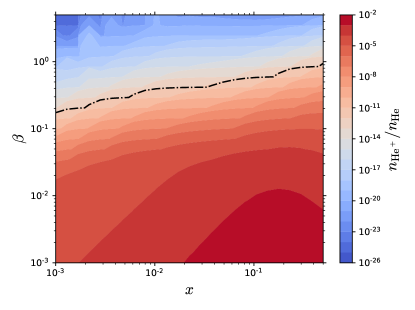
Figure 3: Residual ionization fractions $n_{\mathrm{H^{+}}}/n_{\mathrm{H}}$ (left) and $n_{\mathrm{He^{+}}}/n_{\mathrm{He}}$ (right) of the mirror sector at $z=10$. The dot-dashed contours indicate the SM values: $n_{\mathrm{H^{+}}}/n_{\mathrm{H}}=2.2\times 10^{-4}$ and $n_{\mathrm{He^{+}}}/n_{\mathrm{He}}=1.2\times 10^{-12}$.

We can also understand qualitative features of fig. 3 concerning H recombination. In contrast to He, there is a much stronger variation of $n_{\mathrm{H}}$, which changes by a factor of 60 as $x$ goes from $10^{-3}$ to $0.5$, as compared to only a factor of 2 variation in $n_{\mathrm{He}}$. In particular, for $x\ll 1$ the low density of H is overwhelmed by free electrons, requiring relatively few collisions to recombine such that H may become neutral before He does so. In this situation, for $\beta\sim 1$, H recombination takes place much earlier than for He and it is more efficient than in the SM. But since He recombines very effectively, the number of free electrons available for hydrogen-electron collisions after the freeze-out drops significantly, leading to a much higher ionization fraction than for He. For $\beta\ll 1$, He recombination is very inefficient, leaving a larger number of free electrons to combine with H, and leading to a small ionization fraction. In the region where $x\gtrsim 0.1$, hydrogen and helium number densities are almost equal, and their ionization fractions display a similar qualitative dependence on $\beta$.

II.4 H₂ formation

H₂ is an important molecular species for structure formation since it can cool a primordial gas cloud to a temperature as low as $\sim 200$ K. Even in the SM , a small fraction of H₂ can act as an effective heat sink that drives the collapse of large clouds into stellar objects. Conversely, without H₂, a virialized gas cloud of mirror helium might not cool below a temperature of order $10^{4}$ K (about 1 eV, or roughly 10 % of ionization energy of helium and hydrogen), preventing structure formation.

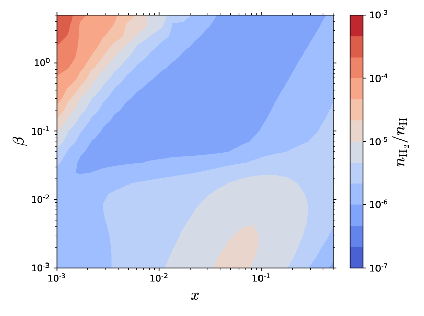
Figure 4: Residual fraction $f_{2}=n_{\mathrm{H_{2}}}/n_{\mathrm{H}}$ produced during mirror recombination at $z=10$. This fraction is higher than the SM value of $n_{\mathrm{H_{2}}}/n_{\mathrm{H}}\simeq 6\times 10^{-7}$ for any ($x,\beta$).

Since H₂ has no dipole moment, it cannot form directly from the collision of two neutral H atoms. Instead, at early times its formation proceeds through the reactions

$$\begin{gathered}\mathrm{H}^{0}+e^{-}\rightarrow\mathrm{H}^{-}+\gamma,\\ \mathrm{H}^{-}+\mathrm{H}^{0}\rightarrow\mathrm{H}_{2}+e^{-}.\end{gathered}$$ (13)

H₂ is always energetically favored at low temperatures, but the low matter density and ionization fractions inhibit its production after recombination. Hence H₂ can only form during recombination, when both $n_{e}$ and $n_{\mathrm{H^{0}}}$ are significant.

Other mechanisms involving H${}_{2}^{+}$ and HeH⁺ are known to contribute to the residual H₂ abundance, but these processes are subdominant Hirata:2006bt . At late times, after the first generations of stars, H₂ formation is catalyzed by dust grains and proceeds more rapidly, but between these epochs the reactions (13) are the only available route.

As was shown in ref. Hirata:2006bt , the production of H₂ depends on the abundance of H^-, which in the steady-state approximation is:

$$X_{\mathrm{H}^{-}}=\frac{k_{7}X_{e}X_{\mathrm{H^{0}}}n_{\mathrm{H}}}{k_{-7}+k_{8}X_{\mathrm{H^{0}}}n_{\mathrm{H}}+k_{9}X_{e}n_{\mathrm{H}}+k_{15}X_{\mathrm{H^{+}}}n_{\mathrm{H}}}.$$ (14)

The rates $k_{i}$ are listed in table B.3.

The residual H₂ abundance is determined by the Boltzmann equation

$$\frac{dX_{\mathrm{H_{2}}}}{dt}=k_{8}X_{\mathrm{H^{0}}}X_{\mathrm{H}^{-}}n_{\mathrm{H}}.$$ (15)

Since both H^- and H₂ attain low abundances, their presence has little effect on the evolution of recombination. We can integrate eq. (15) using the numerical method from the previous subsection. The fraction of $f_{2}^{\prime}=n_{\mathrm{H_{2}}}/n_{\mathrm{H}}$ produced by $z=10$ is illustrated in fig. 4. For reference, the same analysis in the SM yields $f_{2}\simeq 6\times 10^{-7}$. We find that $f_{2}^{\prime}$ is always greater than $f_{2}$, analogously to the higher efficiency of mirror recombination. The degree of enhancement $f^{\prime}_{2}/f_{2}$ depends on the timing of He recombination versus that of H, since H₂ requires both neutral H and free $e^{-}$ for its formation.

When $\beta,x\sim 1$, recombination proceeds similarly as in the SM: He recombines efficiently and prior to H, leaving too few $e^{-}$ for H₂ to form. As $\beta$ decreases, He recombination becomes incomplete and the extra $e^{-}$ density produces more H₂. For $x\ll 1$ but $\beta\sim 1$, H recombines before He, leading to simultaneously high abundances of neutral H and free $e^{-}$. This explains the enhanced H₂ production in fig. 4. If both $x\ll 1$ and $\beta\ll 1$, the two recombinations overlap, leaving fewer $e^{-}$ to produce molecules.

III Mirror matter structure formation

We use the semi-analytical galaxy formation model GALFORM presented in ref. Cole:2000ex to predict structures in the SM . Our analysis parallels that of ref. Ghalsasi:2017jna , but is complicated by the additional chemical elements present in the SM  relative to the simple atomic DM model considered there. In particular, nuclear reactions in the SM  allow for the formation of mirror stars and supernovae whose feedback can impact the collapse of gas clouds.

III.1 Merger tree

Our current understanding of structure formation is that galaxies formed following a bottom-up hierarchy: small halos merged at early times and grew into larger overdense regions. The extended Press-Schechter formalism Press:1973iz ; Bond:1990iw ; Lacey:1993iv , which we summarize here, is an analytic description of the statistical growth and merger history of a halo that reproduces the results of cosmological simulations.

Let $M_{2}$ be the mass of a halo at time $t_{2}$. The mass fraction $f_{12}(M_{1},M_{2})\,dM_{1}$ of $M_{2}$ that was in halos in the interval $\left[M_{1},M_{1}+dM_{1}\right]$ at a time $t_{1}<t_{2}$ is

$$f_{12}\left(M_{1},M_{2}\right)dM_{1} =\frac{1}{\sqrt{2\pi}}\frac{\left(\delta_{\mathrm{c}1}-\delta_{\mathrm{c}2}\right)}{\left(\sigma_{1}^{2}-\sigma_{2}^{2}\right)^{3/2}}$$ (16)

$$\times\exp\left(-\frac{\left(\delta_{\mathrm{c}1}-\delta_{\mathrm{c}2}\right)^{2}}{2\left(\sigma_{1}^{2}-\sigma_{2}^{2}\right)}\right)\frac{d\sigma_{1}^{2}}{dM_{1}}dM_{1},$$

where $\sigma^{2}(M)$ is the variance of the matter power spectrum $P(k)$ inside a sphere of comoving radius $R=(3M/4\pi\rho_{m})^{1/3}$, extrapolated linearly to $z=0$, and $\delta_{\mathrm{c}}(t)$ is the critical overdensity for gravitational collapse at time $t$, also extrapolated to current times,

$$\delta_{\mathrm{c}}\left(t_{\mathrm{c}}\right)=\frac{1}{D(z_{\mathrm{c}})}\frac{3}{5}\left(\frac{3\pi}{2}\right)^{2/3}\left[\Omega_{\mathrm{m}}\left(z_{\mathrm{c}}\right)\right]^{0.0055}.$$ (17)

The linear growth factor $D(z)$ (set to unity at $z=0$) evolves as

$$D(z)\propto H(z)\int_{z}^{\infty}\frac{1+z^{\prime}}{H(z^{\prime})^{3}}\,dz^{\prime}$$ (18)

and $z_{c}$ is the redshift at time $t_{c}$. In a matter-dominated universe $D(z)$ is exactly equal to the scale factor $a=(z+1)^{-1}$, but here we also account for dark energy, which becomes important as $z\to 0$.

Taking $t_{2}=t_{1}+dt$ with $dt$ arbitrarily small, eq. (16) becomes

$$\frac{df_{12}}{dt}=\frac{1}{\sqrt{2\pi}}\frac{1}{\left(\sigma_{1}^{2}-\sigma_{2}^{2}\right)^{3/2}}\frac{d\delta_{\mathrm{c}1}}{dt}\frac{d\sigma_{1}^{2}}{dM_{1}}.$$ (19)

Therefore the average number of objects in $\left[M_{1},M_{1}+dM_{1}\right]$ that combined during $dt$ to form the halo of larger mass $M_{2}$ is

$$dN=\frac{df_{12}}{dt}\frac{M_{2}}{M_{1}}\,dt\,dM_{1}.$$ (20)

The algorithm presented in refs. Cole:2000ex ; Ghalsasi:2017jna uses eq. (20) to find the progenitors of a halo of mass $M_{2}$ by taking small steps $dt$ backwards in time. The resulting “merger tree” describes the hierarchical formation of the halos observed at $z=0$.

Numerically, one must define a resolution scale $M_{\mathrm{res}}$ below which there is no further tracking of individual halos. The probability that a halo of mass $M_{2}$ splits into halos of masses $M_{1}\in\left[M_{\mathrm{res}},M_{2}/2\right]$ and $(M_{2}-M_{1})$ in a backward step $dt$ is

$$P=\int_{M_{\mathrm{res}}}^{M_{2}/2}\frac{dN}{dM_{1}}\,dM_{1}.$$ (21)

Accretion of objects smaller than $M_{\mathrm{res}}$ also contribute to the growth of the halo during that period. The fraction of mass that is lost to those smaller fragments in the reverse time evolution is

$$F=\int_{0}^{M_{\mathrm{res}}}\frac{dN}{dM_{1}}\frac{M_{1}}{M_{2}}\,dM_{1}.$$ (22)

The algorithm to generate the merger tree is as follows. Starting at redshift $z_{f}$ with a single halo of mass $M_{2}=M_{f}$, a backward time step $dt$ is taken, with $dt$ small enough that $P\ll 1$. A random number $R$ is generated from a uniform distribution between $0$ and $1$. If $R>P$, the halo does not fragment, but still loses a fraction of mass $F$ due to the accretion of matter below the resolution scale. Thus the mass of the halo at the next time step becomes $(1-F)M_{2}$. If $R<P$, the halo splits into two halos of mass $M_{1}$ and $(1-F)M_{2}-M_{1}$ where $M_{1}$ is chosen randomly from the distribution given by eq. 20. These steps are repeated for every progenitor whose mass is above $M_{\rm res}$ until the chosen initial redshift $z_{i}$ is reached.

We used this algorithm to generate 10 merger trees for a final halo mass of $M_{f}=10^{12}\ M_{\odot}$, about the size of the Milky Way. The time interval between $z_{f}=0$ and $z_{i}=10$ was divided into $10^{4}$ logarithmically scaled time steps. The resolution was set to $M_{\mathrm{res}}=3\times 10^{7}\ M_{\odot}$, well below $M_{f}$ but large enough to avoid keeping track of too many halos simultaneously. To minimize possibly large statistical fluctuations, we used the ensemble of merger trees to average over all derived quantities in the end. Inspection of the individual trees indicated that 10 was more than sufficient to avoid spurious effects of outliers.

Neither the distribution nor the nature of matter inside the halos affects the evolution of the merger tree. Therefore the algorithm described above is completely model-independent, to the extent that matter overdensities are Gaussian. This allows us to use the same 10 merger trees in scanning over all values of $x$ and $\beta$ for structure formation. However $P(k)$ depends on the nature of dark matter, which in turn affects the variance $\sigma^{2}(M)$ in eqs. (16,19-22). For simplicity, we computed $\sigma^{2}$ with Colossus Diemer:2017bwl , but this package assumes a $\Lambda$CDM cosmology. For self-consistency, it is necessary to verify that $P(k)$ and its variance $\sigma^{2}$ do not differ too much from their standard cosmology expressions in the presence of a mirror sector. We discuss this issue below.

III.2 Mirror Silk damping

In the early universe, photons and baryons are tightly coupled, making the mean free path of photons $\lambda_{\gamma}$ negligible, but at the onset of recombination $\lambda_{\gamma}$ becomes significant. Photons can then diffuse out of overdense regions, effectively damping perturbations on scales smaller than the Silk scale $\lambda_{D}$, which we derive below. In the SM, the mass scale corresponding to the Silk length is $M_{D}\sim 10^{12}\ M_{\odot}$ Kolb:1990vq , about the mass of the Milky Way halo. Structure formation below this scale is strongly inhibited, unless a significant component of CDM allows small-scale perturbations to grow.

Mirror matter can be similarly affected by collisional damping. Since we observe structures on scales smaller than $M_{D}$, Silk damping sets a lower bound on the amount of ordinary CDM required for the mirror model to agree with current data. A full analysis of cosmological perturbations, acoustic oscillations and the matter power spectrum is outside the scope of this work. However, the equations presented in the previous section depend on $P(k)$ through its variance $\sigma^{2}(M)$. We must therefore check that $P(k)$ is not too different from its $\Lambda$CDM value. Many effects could alter $P(k)$, like extra oscillations on scales smaller than the sound horizon of the mirror matter plasma Cyr-Racine:2013fsa , but Silk damping has the largest impact on our structure formation analysis. In particular, small-scale perturbations must be able to grow sufficiently for galaxy formation to proceed hierarchically. Hence we estimate the size of the SM  counterpart of the damping scale, $\lambda^{\prime}_{D}$, and its implications for the growth of SM  density perturbations.

III.2.1 Mirror Silk scale

One can estimate the SM  Silk scale as follows Kolb:1990vq . The mean free path of SM  photons at low temperatures is

$$\lambda_{\gamma^{\prime}}=\frac{1}{n_{e}\sigma_{T}}=\frac{1}{\xi_{e}n_{N}\sigma_{T}},$$ (23)

where $\xi_{e}\equiv n_{e}/n_{N}$ is the ionization fraction during H and He${}^{+}\to$ He⁰ recombination. During an interval $\Delta t$, a photon experiences $N=\Delta t/\lambda_{\gamma^{\prime}}$ collisions. The average comoving distance $\Delta r$ traveled in this time is that of a random walk with a characteristic step of length $\lambda_{\gamma^{\prime}}/a$,

$$(\Delta r)^{2}=N\frac{\lambda_{\gamma^{\prime}}^{2}}{a(t)^{2}}=\frac{\lambda_{\gamma^{\prime}}\Delta t}{a(t)^{2}}.$$ (24)

Taking the limit $\Delta t\rightarrow 0$ and integrating until recombination gives

$$\begin{split}\lambda_{D}^{\prime 2}&=\int_{0}^{t_{\mathrm{rec}}}\frac{\lambda_{\gamma^{\prime}}}{a(t)^{2}}dt\\ &\simeq-\lambda_{\gamma^{\prime}}(z^{\prime}_{\mathrm{rec}})\ \left(1+z^{\prime}_{\mathrm{rec}}\right)^{3}\int^{\infty}_{z_{\mathrm{rec}}^{\prime}}\frac{1}{1+z}\left(\frac{dt}{dz}\right)dz,\end{split}$$ (25)

using the fact that $\lambda_{\gamma^{\prime}}$ scales as $n_{N}^{-1}\sim a^{3}$ and approximating $\xi_{e}$ as constant during the period where $\lambda_{\gamma^{\prime}}$ is large.

Recalling that the redshift of mirror recombination is $z_{\mathrm{rec}}^{\prime}\simeq 1100/x$, this occurs before matter-radiation equality ($z_{\mathrm{eq}}=3365$) for $x\lesssim 0.3$, and during the early matter-dominated era otherwise. For simplicity, consider the case $x\ll 0.3$ so that mirror recombination completes during the radiation-dominated era when $t\sim(1+z)^{-2}$. Eq. (25) then reduces to

$$\lambda_{D}^{\prime 2}\simeq\frac{2}{3}t_{\mathrm{rec}}^{\prime}\ \lambda_{\gamma^{\prime}}(z_{\mathrm{rec}}^{\prime})\ (1+z_{\mathrm{rec}}^{\prime})^{2},\ \quad x\ll 0.3.$$ (26)

In the case where recombination occurs much later than $z_{\mathrm{eq}}$ (like in the SM), we would obtain the same expression, without the primes, up to the numerical coefficient Kolb:1990vq . This implies that $\lambda^{\prime}_{D}\ll\lambda_{D}$, unless $\beta$ is very small and the mirror matter plasma is diluted before recombination.

To further quantify $\lambda^{\prime}_{D}$, we note that at early times when vacuum energy is negligible so that $\Omega_{m}+\Omega_{\mathrm{rad}}=1$, $t(z)$ is given by

$$\begin{split}t(z)&=\frac{2}{3H_{0}\sqrt{\Omega_{\mathrm{m,0}}}}\frac{1}{(1+z_{\mathrm{eq}})^{3/2}}\\ &\times\left[2+\left(\frac{1+z_{\mathrm{eq}}}{1+z}-2\right)\sqrt{\frac{1+z_{\mathrm{eq}}}{1+z}+1}\right].\end{split}$$ (27)

which for $z\gg z_{\mathrm{eq}}$ simplifies to

$$t(z\gg z_{\mathrm{eq}})\simeq\frac{1}{2H_{0}\sqrt{\Omega_{\mathrm{m,0}}}}\frac{\sqrt{1+z_{\mathrm{eq}}}}{(1+z)^{2}}.$$ (28)

Then eq. (26) can be rewritten in terms of $x(\ll 1)$ and $\beta$ as

$$\lambda_{D}^{\prime 2}\simeq\frac{8\pi G}{9H_{0}^{3}\sqrt{\Omega_{m}}\Omega_{b}}\left(\frac{\overline{m_{N}}x^{3}}{\xi_{e}\sigma_{T}\beta}\right)\frac{\sqrt{1+z_{\mathrm{eq}}}}{(1+z_{\mathrm{rec}})^{2}}.$$ (29)

(recall eq. (7) for $\overline{m_{N}}$), where we used $\xi_{e}\sim 0.1$ at the time of recombination. Hence $\lambda^{\prime}_{D}$ scales as $(x^{3}/\beta)^{1/2}$. For larger values of $x$, $z_{\mathrm{rec}}^{\prime}$ is close to $z_{\mathrm{eq}}$ and we cannot assume a fully matter- or radiation-dominated universe to compute the integral of eq. (25); nevertheless we verified that eqs. (26,27) are accurate to within several percent even for $x>0.3$.

III.2.2 Growth of MS perturbations

The previous estimate for $\lambda^{\prime}_{D}$ allows us to predict the growth of density perturbations in the SM . Consider a mirror baryonic overdensity $\delta_{b^{\prime}}(k)=(\rho_{b^{\prime}}(k)-\overline{\rho_{b^{\prime}}})/\overline{\rho_{b^{\prime}}}$ on a scale $\lambda=\pi/k$. Assuming primordial perturbations are adiabatic, we have $\delta_{b^{\prime}}=\delta_{c}$ at early times ($z\gg z_{\mathrm{eq}}$). $\delta_{c}$ remains nearly constant prior to matter-radiation equality (ignoring small logarithmic growth of subhorizon modes). However Silk damping suppresses $\delta_{b^{\prime}}(k)$ by a factor $\sim\exp\left(-k^{2}/k_{D}^{\prime 2}\right)$ after recombination MBW:2010 , where $k_{D}^{\prime}=\pi/\lambda_{D}^{\prime}$.

For very small values of $\beta$, the SM  constitutes only a small fraction of DM and the power spectrum is not significantly affected by mirror Silk damping. Therefore in what follows we only consider $\beta\gtrsim 0.1$, where consequently $\lambda_{D}\gg\lambda^{\prime}_{D}$. The analysis below focuses on scales sufficiently small so that SM baryonic perturbations are always negligible compared to CDM and SM  overdensities.

Starting at $z=z_{\mathrm{eq}}$, both the CDM and mirror components grow linearly according to the cosmological perturbation equations Naoz:2005pd

$$\ddot{\delta}_{c}+2H\dot{\delta}_{c}=\frac{3}{2}H_{0}^{2}\frac{\Omega_{\mathrm{DM}}}{a^{3}}\left(f_{b^{\prime}}\delta_{b^{\prime}}+f_{c}\delta_{c}\right)$$ (30)

$$\ddot{\delta}_{b^{\prime}}+2H\dot{\delta}_{b^{\prime}}=\frac{3}{2}H_{0}^{2}\frac{\Omega_{\mathrm{m}}}{a^{3}}\left(f_{b^{\prime}}\delta_{b^{\prime}}+f_{c}\delta_{c}\right)-\frac{k^{2}}{a^{2}}c_{s}^{2}\delta_{b^{\prime}},$$ (31)

where $f_{i}\equiv\Omega_{i}/\Omega_{\mathrm{DM}}$ are the fractions of the total DM density, such that $f_{b^{\prime}}+f_{c}=1$. We omit the equation for $\delta_{b}$, which is highly damped on small scales.

Recall that mirror baryons recombine before $z_{\mathrm{eq}}$ for $x\lesssim 0.3$. Subsequently the SM  pressure drops precipitously, which means that its sound speed $c^{\prime}_{s}\sim 0$ at matter-radiation equality. Even before SM  recombination, $c_{s}^{\prime 2}$ is suppressed by a factor $\sim x^{4}$ compared to the SM $c_{s}^{2}$, due to the low SM  temperature Berezhiani:2000gw ; Ignatiev:2003js . To a first approximation we can therefore ignore the pressure term in eq. (31) for all values of $x$. We can then combine the two ODEs into

$$\ddot{\delta}^{\prime}+2H\dot{\delta}^{\prime}=\frac{3}{2}H_{0}^{2}\frac{\Omega_{\mathrm{DM}}}{a^{3}}\delta^{\prime}$$ (32)

where $\delta^{\prime}=(f_{b^{\prime}}\delta_{b^{\prime}}+f_{c}\delta_{c})$ is the total matter perturbation; the CDM and mirror matter perturbations evolve together during the matter-dominated era and their ratio remains constant. The growing mode grows as $\delta^{\prime}\sim a$, so that at small redshifts

$$\begin{split}\delta^{\prime}(z)=&\delta^{\prime}(z_{\mathrm{eq}})\left(\frac{1+z_{\mathrm{eq}}}{1+z}\right)\\ =&\delta_{c}(z_{\mathrm{eq}})\,\left(1-f_{b^{\prime}}(1-e^{-k^{2}/k_{D}^{\prime 2}})\right)\left(\frac{1+z_{\mathrm{eq}}}{1+z}\right),\end{split}$$ (33)

where we combined the initial abadiatic condition $\delta_{b^{\prime}}=\delta_{c}$ with the exponential Silk damping. Therefore we see that Silk damping suppresses small scale matter perturbations by an additional factor of roughly

$$\mathcal{F}_{D}=\left(1-\frac{\beta\Omega_{b}}{\Omega_{\mathrm{DM}}}(1-e^{-k^{2}/k_{D}^{\prime 2}})\right)$$ (34)

compared to standard cosmology.

III.2.3 Effect on the merger tree evolution

To verify that our merger tree evolution is not significantly altered by the suppression of $P(k)$ on small scales, we applied the Silk damping factor $\mathcal{F}_{D}$ to the $\Lambda$CDM matter power spectrum and we computed the variance $\sigma^{2}(M)$ and the integral $P$ of eq. (21) for a Milky Way-like halo ($M_{2}=10^{12}$ M_⊙) with this extra feature.

The value of $P$ is the probability for a merger to happen and it is roughly inversely proportional to the lifetime of large halos $t_{\mathrm{halo}}$, which we will properly define later. The accretion rate $F$ given by eq. (22) also affects $t_{\mathrm{halo}}$, but for large halos it represents such a small fraction of the total mass that we can ignore it. Let $P_{D}$ be the value of the integral of eq. (21) computed with the damped power spectrum. We expect that the lifetime should scale as $t_{\mathrm{halo}}\sim P/P_{D}$.

In our 10 merger trees, the average lifetime of the Milky Way halo is 6.9 Gyr with a relative standard deviation of 21.5 %. To ensure the self-consistency of our analysis, we demand that the Silk damping does not change the average lifetime by more than $2\sigma$, or 43 %. In other words, our analysis is valid only if $0.57<P/P_{D}<1.43$; outside this region we cannot trust our conclusions because the merger trees would be too drastically affected by the damping effects.

We find that two regions above $\beta\gtrsim 3.7$ must be excluded from our analysis: for $0.02\lesssim x\lesssim 0.12$, $t_{\mathrm{halo}}$ would be much longer than the estimate we obtained using the $\Lambda$CDM power spectrum; whereas for $x\gtrsim 0.2$, the halo lifetime in the presence of mirror matter would be too small. These regions are illustrated with our results on fig. 7.

Note that the different behaviors in these two regions come from two competing effects in eq. (19): both $\left|d\sigma_{1}^{2}/dM_{1}\right|$ and $(\sigma_{1}^{2}-\sigma^{2})^{3/2}$ are suppressed by the collisional damping, but the latter effect dominates for large values of $x$, when the Silk scale is large. Interestingly, those effects cancel out around $x\simeq 0.15$ and we can still use our structure formation analysis to constrain the scenario where mirror matter makes up all DM in this region. Fortunately, the high temperature region also corresponds to the parameter space that is more likely to be constrained by cosmological observables like the CMB or the matter power spectrum. Ref. Ciarcelluti:2010zz already constrained $x\lesssim 0.3$ if mirror matter were to make up all DM.

III.3 Virialization and cooling

Once linear matter perturbations exceed the critical overdensity $\delta_{\mathrm{c}}$ (eq. (17)) they collapse gravitationally into a virialized halo whose average overdensity is MBW:2010 :

$$\Delta_{\mathrm{vir}}(z)=\frac{18\pi^{2}+82\,y-39\,y^{2}}{\Omega_{\mathrm{m}}(z)},$$ (35)

with $y=\Omega_{\mathrm{m}}(z)-1$. Since mirror baryonic matter is not pressureless, this collapse leads to accretion shocks that heat the gas to a temperature of roughly MBW:2010 ; DAmico:2017lqj :

$$T_{M}=(\gamma-1)\ T_{\mathrm{vir}}=(\gamma-1)\ \frac{1}{2}\frac{GM\mu}{r_{\mathrm{vir}}},$$ (36)

where $\gamma$ is the adiabatic index of the gas, $\mu$ is the mean molecular mass, $M$ is the total mass of the halo (including the CDM component) and $r_{\mathrm{vir}}$ is the virial radius. We define $r_{\mathrm{vir}}$ as the radius of a sphere inside which the average overdensity is equal to $\Delta_{\mathrm{vir}}$. For simplicity, we will assume the gas is purely monatomic, which sets $\gamma=5/3$.

The temperature of a virial halo is always much greater than the temperature of the matter background. This means the baryonic pressure $P=\rho T/\mu$ becomes nonnegligible and prevents further collapse of mirror matter. In order for galaxies to form, mirror baryons must radiate energy, which is why structure formation is impossible without an efficient cooling mechanism.

Let $\mathcal{C}_{i}=-du/dt$ be the cooling rate of a given process $i$, where $u$ is the energy density of the gas ($\mathcal{C}_{i}$ is positive if the energy is lost). If several reactions contribute to the total $\mathcal{C}$, we can define the cooling timescale as

$$t_{\mathrm{cool}}(r)=\frac{3}{2}\frac{n(r)T_{M}}{\sum_{i}\mathcal{C}_{i}(r,T_{M})}.$$ (37)

where $n(r)$ is the number density of all chemical species combined. Therefore $t_{\mathrm{cool}}$ is roughly the time required for the gas to radiate all its kinetic energy. Since the gas is not homogeneous, the cooling timescale decreases as we move further away from the center of the halo. We describe the various contributions to $\mathcal{C}$ MBW:2010 ; Cen:1992zk ; Grassi:2013lha ; 1979ApJS…41..555H in appendix B.

To compute the cooling rates and timescale, one must also specify the number density $n_{i}$ of each chemical species. In general, their relative abundances are determined by rate equations of the form Grassi:2013lha

$$\frac{dn_{i}}{dt}=\sum_{j\in F_{i}}\left(k_{j}\prod_{r\in R_{j}}n_{r}^{(j)}\right)-\sum_{j\in D_{i}}\left(k_{j}\prod_{r\in R_{j}}n_{r}^{(j)}\right),$$ (38)

where $F_{i}$ and $D_{i}$ are the sets of reactions $R_{j}$ that form and destroy the $i$th species and $n_{r}^{j}$ is the number density of each reactant in $R_{j}$. The coefficients $k_{j}$ set the rate of each reaction and usually depend on the temperature of the system. If the right-hand-side of eq. (38) vanishes for a given species, the reaction is in collisional equilibrium, or steady state. If all processes are two-body reactions, the steady-state density is given by

$$n_{i}=\frac{\sum\limits_{j\in F_{i}}k_{j}n_{1}^{(j)}n_{2}^{(j)}}{\sum\limits_{j\in D_{i}}k_{j}n_{d}^{(j)}}.$$ (39)

The cooling mechanisms depend on the abundances of eight chemical species: H⁰, H⁺, H^-, H₂, He⁰, He⁺, He⁺⁺ and $e^{-}$ . In the steady-state approximation, the network eq. (39) is usually underdetermined, but one can solve it if 1) the total nuclear density $n_{N}=n_{\mathrm{H}}+n_{\mathrm{He}}$ satisfies eq. (8); 2) the total He-H number ratio $X_{\mathrm{He}}=n_{\mathrm{He}}/n_{\mathrm{H}}$ satisfies eq. (5) (assuming nuclear reactions in stars do not strongly affect $X_{\mathrm{He}}$); 3) matter is neutral, which implies $n_{e}\simeq n_{\mathrm{H^{+}}}+n_{\mathrm{He^{+}}}+2n_{\mathrm{He^{++}}}$ (since the density of H^- is negligible). The reactions considered in our simplified chemical network and their rates are given in table B.3.

However, the steady-state approximation tends to break down at low temperature/densities; if the timescale of a given reaction $t_{r}\sim(k_{r}n)^{-1}$ is smaller than the dynamical timescale of the system $t_{\mathrm{dyn}}\sim(G\rho)^{-1/2}$, the chemical species cannot reach collisional equilibrium. This is most likely to occur at early times in small halos with low density and temperature. At $z=10$ the $t_{\mathrm{dyn}}$ corresponding to the virial overdensity is $\sim 0.2$ Gyr. Taking $n\sim 1$ cm^-3 — roughly the central density in a $3\times 10^{7}$ M_⊙ halo at this epoch — we can check that H₂, H⁺ and He⁺ respectively come into collisional equilibrium at about 4,000 K, 9,000 K and 15,000 K. Below those critical temperatures we take the abundances of each species to be their relic densities after recombination, as determined by Recfast++ (section II.3).

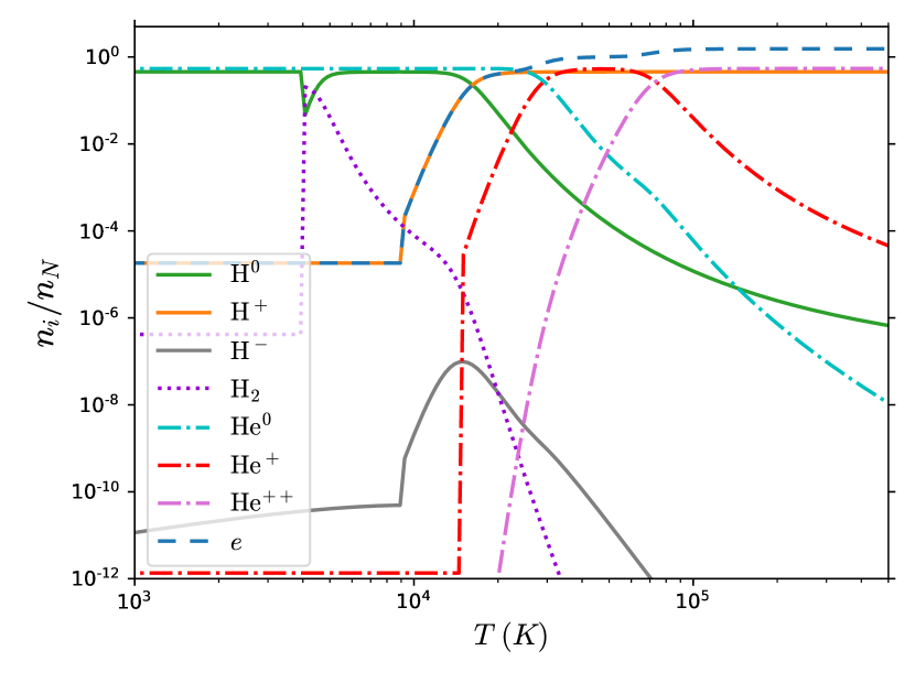
Figure 5: Example of the relative abundance of each chemical species at $z=10$ as a function of the temperature of the gas. We used the benchmark parameters $x=0.1$ and $\beta=1$.

In reality the chemical species evolve toward their equilibrium values during shock heating; the true densities therefore lie between the equilibrium and the freeze-out values, but this difference has a negligible impact on the cooling rates at high $z$, as well as on the overall evolution of the galaxy.   Fig. 5 illustrates the evolution of each chemical species with the temperature at $z=10$ with parameter $x=0.1$ and $\beta=1$. The abrupt transitions result from the approximations described here, and would be smoothed out by fully solving eqs. (38), but with no appreciable effect on the consequent formation of structure.

III.4 Cloud collapse and star formation

As the cloud of mirror matter that fills the halo loses energy, its pressure drops and it is no longer sufficient to counteract the self-gravity of the gas. The cloud starts collapsing and fragments in overdense regions. If the cooling mechanism is very efficient, the collapse will occur on a characteristic timescale set by the free-fall time,

$$t_{\mathrm{ff}}(r)=\sqrt{\frac{3\pi}{32G\rho_{r}}}.$$ (40)

In this expression $\rho_{r}$ is the average matter density inside a sphere of radius $r$.

As the gas gets denser, the horizon of sound waves becomes increasingly smaller and matter cannot remains isothermal on scale larger than the Jeans length Ghalsasi:2017jna ; CarrollOstlie ,

$$\lambda_{J}=\sqrt{\frac{15kT}{4\pi G\mu\rho}}.$$ (41)

Below this scale the gas cannot fragment further. This sets the minimal mass of fragments that result from the collapse:

$$M_{J}=\frac{4\pi\rho}{3}\lambda_{J}^{3}.$$ (42)

By evaluating the Jeans mass at the final density and temperature we can obtain a rough estimate of the mass of the primordial stars of mirror matter. Following DAmico:2017lqj , we used Krome Grassi:2013lha to study the evolution of the temperature and the density of a collapsing cloud of mirror matter gas. Krome assumes the cloud is in a free fall,

$${\dot{n}\over n}\sim{1\over t_{\mathrm{ff}}}$$ (43)

(recall eq. (40) for $t_{\mathrm{ff}}$), and solves the out-of-equilibrium rate equations (38). The temperature evolves as Grassi:2013lha

$$\frac{\dot{T}}{T}=(\gamma-1)\left(\frac{\dot{n}}{n}+\frac{\mathcal{H}-\mathcal{C}}{nkT}\right),$$ (44)

where the cooling rate is $\mathcal{C}=\sum_{i}\mathcal{C}_{i}$ and $\mathcal{H}$ is the heating rate. The heating rate is negligible in the optically thin limit because photons exit the cloud, but as the gas becomes denser we must include it in our calculations. Recall that $\gamma=5/3$.

In the absence of cooling, eq. (44) shows that the temperature of the cloud will increase as it collapses. However if the cooling processes dominate, the collapse continues unimpeded as $T$ (and pressure) decreases. Eventually the gas becomes optically thick and the cooling becomes ineffective; at this point the approximation (43) of free-fall evolution breaks down and the cloud can only collapse adiabatically, which tends to increase the Jeans mass. In reality, the angular momentum of the cloud becomes nonnegligible before then and the mass of the fragments is determined by criteria other than eq. (42).

We focus on the cloud collapse inside the MW halo at $z=10$, which according to the merger trees has an average mass $M\simeq 8\times 10^{8}$ M_⊙ and central density $n\sim 1$ cm^-3. It is assumed that the collapse can always happen, independently of $x$ and $\beta$, and that the fragments can cool to $\sim 10$ % of $T_{M}$ (see eq. (36)) before collapsing. In section III.5 we will verify the values of $(x,\beta)$ for which cooling is really efficient enough for the cloud to collapse. In such a case $T$ drops to values $\ll T_{M}$ before the density increases significantly. Then our assumptions are self-consistent and allow for estimating the mass of primordial stars independently of $\beta$; dependence on $x$ remains since it affects the chemical abundances.

Fig. 6 shows the evolution of the temperature from eq. (44) during the collapse for several values of $x$ and for the SM. It reveals that smaller values of $x$ lead to more efficient cooling, since more H₂ can form. Interestingly, even when the hydrogen fraction is small, H₂ cooling can reduce $T$ to $\sim{\rm few}\times 100$ K very rapidly. We evaluated the Jeans mass at the minimum $T$ (near $n\sim 200$ cm^-3) to estimate the mass $M_{*}^{\prime}$ ($M_{*}$) of the fragments in the SM  (SM). After this point, the cloud collapses quasi-adiabatically and the rise of $T$ slows the decrease of the Jeans mass. This point allows us to set an upper limit on the final fragment mass $M_{*}^{\prime}$ rather than evaluating it accurately, which is impossible in our simplified analysis without angular momentum.

Note that this oversimplification is not an issue, because we are only interested in the ratio $\zeta\equiv M_{*}^{\prime}/M_{*}$ of the fragment mass in the SM  and in the SM, which wouldn’t change much if we evaluated eq. 42 at another point of the $n\!-\!T$ diagram. This ratio gives a rough approximation of how the mass of the mirror stars scales compared to the visible ones, which allows us to estimate their lifetimes and their supernova feedback on structure formation. Fig. 6 also illustrates the value of $\zeta$ for all values of $x$. It is apparent that $\zeta>1$ for all values of $x$, indicative of the lower cooling efficiency in the SM  (from suppressed H abundance) leading to less fragmentation of gas clouds.

We should emphasize that this estimate of $\zeta$ is only valid for primordial stars as we do not include any element heavier than He in our analysis. In reality, it is possible that the short-lived He-dominated stars in the SM  produce metals at a much higher rate than in the SM. Since metals are easier to ionize, their presence can significantly increase the cooling rate and the fragmentation inside a gas cloud. We leave this analysis for a future study.

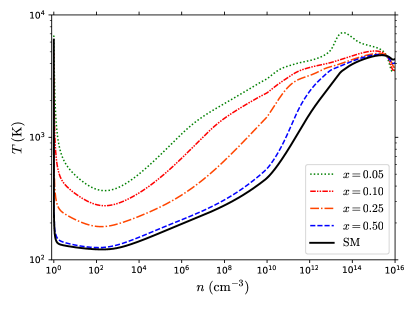
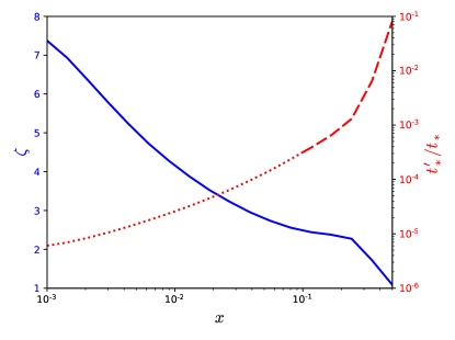
Figure 6: Left: Temperature evolution during the cloud collapse of a gas fragment at $z=10$ in a Milky Way-like halo for values of $x$ increasing from top to bottom, including the SM ($x=1,Y=0.24$). Evaluating eq. (42) at the temperature minimum of each curve gives an estimate of the mass of primordial stars. Right: Ratio $\zeta$ of the minimal fragment mass in the

SM

 relative to the SM (blue, solid) and ratio of the characteristic stellar lifetimes (red, dashed+dotted). The dotted curve illustrates the extrapolation of eq. (III.4) outside the fit interval of ref. Berezhiani:2005vv .

Unlike ordinary matter, mirror stars are usually He-dominated, which has important consequences for their evolution, notably their lifetime $t_{*}$. In the SM, the H-burning phase constitutes most of the lifetime of stars, with the post-main sequence evolution contributing only about 10 % of $t_{*}$. In the SM , with much less H to burn, stars quickly transition to the later stages of their evolution.

We note that the average mass for visible stars can be estimated using the initial mass function (IMF):

$$M_{*}=\int_{0.08\,M_{\odot}}^{100\,M_{\odot}}m\,\phi(m)\,dm\simeq 0.3\ M_{\odot},$$ (45)

where $\phi(m)\propto m^{-2.35}$ is the Salpeter IMF MBW:2010 ; 1955ApJ…121..161S normalized such that its integral over the mass range of stable stars ($0.08\ M_{\odot}<m<100\ M_{\odot}$) is 1. Hence we take the characteristic stellar mass in the SM  to be $M_{*}^{\prime}=\zeta\times(0.3$ M${}_{\odot})$. Ref. Berezhiani:2005vv studied the dependence of $t_{*}$ on the He fraction and the mass of stars. Using their fit results, we estimate the scaling of typical lifetimes of SM  stars by comparison to the SM:

$$\log_{10}\left(\frac{t_{*}^{\prime}}{t_{*}}\right) \simeq 0.74-2.86Y^{\prime}-0.94Y^{\prime 2}-4.77\log_{10}\zeta$$

$$+0.99(\log_{10}\zeta)^{2}+1.34Y^{\prime}\log_{10}\zeta$$ (46)

$$+0.29Y^{\prime 2}\log_{10}\zeta-0.28Y^{\prime 2}(\log_{10}\zeta)^{2}.$$

(recall that $\zeta=M^{\prime}_{*}/M_{*}$).

The ratios $\zeta$ and $t^{\prime}_{*}/t_{*}$ are plotted in figure 6(right) as a function of $x$. $t_{*}^{\prime}/t_{*}$ will be used to estimate the supernova feedback of SM  stars on the formation of dark galactic structures in section III.5.1. We note that eq. (III.4) is only valid up to $Y^{\prime}=0.8$ ($x\simeq 0.1$), so our estimate of the stellar lifetime for $x\lesssim 0.1$ is likely to be too small. However, in this range one nevertheless expects that $t^{\prime}_{*}/t_{*}\ll 1$. In section III.5.1 we will show that the main consequence of such short lifetimes is that supernova feedback favors star production over the formation of cold gas clouds in the mirror galactic disk, whereas in section IV we show that star formation is already maximally efficient at $x=0.1$; hence our results our not sensitive to the precise value of $t^{\prime}_{*}/t_{*}$ at lower temperatures, and it is safe to use eq. (III.4) for $Y^{\prime}>0.8$.

III.5 Mirror galaxy formation

We now have the necessary ingredients for studying the formation of a dark galaxy using the GALFORM model Cole:2000ex . The steps to be carried out for implementing it are described as follows.

The SM  matter is divided into three components: the hot gas component, the spheroidal bulge fraction and the disk fraction. The bulge and the disk together form the SM  galaxy. The disk fraction is further subdivided into two components: active stars and cold gas clouds. Star formation is highly suppressed in the bulge so such a subdivision is not needed there. The remaining matter component is CDM. Visible baryons are omitted from our analysis for simplicity and since GALFORM is not set up to properly account for their gravitational interaction with the SM .   Instead, we include the visible baryons into the CDM fraction, so that $\Omega_{m}=\Omega_{c}+\Omega_{b^{\prime}}$.

CDM is assumed to have an NFW density profile,

$$\rho_{c}(r)=\frac{(\Omega_{c}/\Omega_{m})(\Delta_{\mathrm{vir}}\rho_{\mathrm{crit}}/3)}{\left[\ln(1+c)-\cfrac{c}{1+c}\right]\cfrac{r}{r_{\mathrm{vir}}}\left(\cfrac{r}{r_{\mathrm{vir}}}+\cfrac{1}{c}\right)^{2}}.$$ (47)

The virial radius $r_{\mathrm{vir}}$ and overdensity $\Delta_{\mathrm{vir}}$ were defined in section III.3. $c$ is the NFW concentration and sets the size of the central region of the profile. The procedure to find $c$ for a given halo mass at a given redshift is described in the appendix of ref. Navarro:1996gj . The CDM profile remains constant throughout the lifetime of the halo.

SM

matter is further assumed to form a hot gas cloud with an isothermal density profile,

$$\rho_{b^{\prime}}(r)=\frac{f_{\mathrm{hot}}(\Omega_{b^{\prime}}/\Omega_{m})(\Delta_{\mathrm{vir}}\rho_{\mathrm{crit}}/3)}{\left[1-\cfrac{r_{0}}{r_{\mathrm{vir}}}\tan^{-1}\left(\cfrac{r_{\mathrm{vir}}}{r_{0}}\right)\right]\left(\left(\cfrac{r}{r_{\mathrm{vir}}}\right)^{2}+\left(\cfrac{r_{0}}{r_{\mathrm{vir}}}\right)^{2}\right)}.$$ (48)

The hot gas fraction $f_{\mathrm{hot}}=1$ for all newly formed halos, but $f_{\mathrm{hot}}$ decreases as the gas cools and collapses. The core radius $r_{0}$ is initially related to the NFW concentration as $r_{0}/r_{\mathrm{vir}}=1/(3c)$, but as the gas cools, $r_{0}$ increases such that the density and pressure at $r_{\mathrm{vir}}$ remain unaffected. This is impossible in the limit where a large fraction of the gas cools, so we set an upper limit of $r_{0}=15r_{\mathrm{vir}}$ to avoid a numerical divergence as $r_{0}\to\infty$. In this limit $(r/r_{\mathrm{vir}})^{2}\ll(r_{0}/r_{\mathrm{vir}})^{2}$ and the density profile becomes essentially homogeneous. We truncate both profiles $\rho_{b^{\prime}}(r)$ and $\rho_{c}(r)$ at $r_{\mathrm{vir}}$.

III.5.1 Disk formation

The GALFORM algorithm simulates structure formation beginning at redshift $z=10$, taking as input the merger trees described above, and evolving forward in time using logarithmically spaced time steps $\Delta t$. Halo evolution is simulated semi-analytically until the present, $z=0$. The lifetime of the halo $t_{\mathrm{halo}}$ is defined to be the time it takes to double in mass, whether by matter accretion or by mergers.

The halo is modeled using spherical shells plus a disk component. At the beginning (or end) of each time step, two characteristic radii must be computed: the cooling radius $r_{\mathrm{cool}}$ and the free-fall radius $r_{\mathrm{ff}}$. These are respectively the maximal distances such that the cooling timescale $t_{\mathrm{cool}}$ (eq.  (37)) and the free-fall timescale (eq. (40)) are smaller than the elapsed time since the beginning of the halo’s lifetime, $t-t_{\mathrm{halo}}$. Hence the radius $r_{\mathrm{acc}}=\min(r_{\mathrm{cool}},r_{\mathrm{ff}})$ is the maximum distance to which the gas has had time to cool down and accrete into compact objects.

The values of $r_{\mathrm{acc}}$ before and after the time step $\Delta t$ delimit a spherical shell of width $\Delta r_{\mathrm{acc}}$ that contains mass $\Delta M_{\mathrm{acc}}$ of hot mirror matter gas. As shown in appendix B of ref. Cole:2000ex , this accreted matter determines how the masses of the hot gas $M_{\mathrm{hot}}$ and the disk $M_{\mathrm{disk}}$ change during that time step:

$$\Delta M_{\mathrm{disk}} =\Delta M_{\mathrm{cold}}+\Delta M_{*}$$ (49)

$$\Delta M_{\star} =M_{\mathrm{cold}}^{0}\frac{1-R}{1-R+B}\left[1-e^{-\Delta t/\tau_{\mathrm{eff}}}\right]$$ (50)

$$-\Delta M_{\mathrm{acc}}\frac{\tau_{\mathrm{eff}}}{\Delta t}\frac{1-R}{1-R+B}\left[1-\frac{\Delta t}{\tau_{\mathrm{eff}}}-e^{-\Delta t/\tau_{\mathrm{eff}}}\right]$$

$$\Delta M_{\mathrm{cold}} =\Delta M_{\mathrm{acc}}-\frac{1-R+B}{1-R}\Delta M_{\star}$$ (51)

$$\Delta M_{\mathrm{hot}} =-\Delta M_{\mathrm{acc}}+\frac{B}{1-R}\Delta M_{\star}.$$ (52)

Here $M_{\mathrm{cold}}$ and $M_{*}$ are the masses of the cold gas and stellar components of the disk, and $M_{\mathrm{cold}}^{0}$ is the cold gas mass at the beginning of the time step. $R$ is the fraction of mass recycled by stars (e.g., stellar winds that contribute to the cold gas component of the disk) and $B$ parametrizes the efficiency of the supernova feedback that heats the cold gas fraction.

The effective mirror star formation timescale is $\tau_{\mathrm{eff}}=\tau_{*}^{\prime}/(1-R+B)$. To determine $\tau_{*}^{\prime}$, one can assume that the star formation rate is in equilibrium with the stellar death rate (the inverse of the average stellar lifetime). Then the ratio of star formation timescales $\tau_{*}^{\prime}/\tau_{*}$ in the SM  and in the SM is equal to the ratio of the characteristic stellar lifetimes $t_{*}^{\prime}/t_{*}$, eq. (III.4),

$$\tau_{*}^{\prime}\simeq\left(\frac{t_{*}^{\prime}}{t_{*}}\right)\tau_{*}=200\frac{r_{D}}{V_{D}}\left(\frac{t_{*}^{\prime}}{t_{*}}\right)\left(\frac{V_{D}}{200\ \mathrm{km/s}}\right)^{-1.5}.$$ (53)

Following ref. Cole:2000ex , we take $R=0.31$ and $B=\left(V_{\mathrm{D}}/(200\ \text{km/s})\right)^{-2}$, where $V_{\mathrm{D}}=(GM_{r_{D}}/r_{D})^{1/2}$ is the circular velocity at the half-mass radius $r_{D}$ of the galactic disk. Assuming the disk has an exponential surface density, its half-mass radius can be estimated as $r_{D}=1.19\lambda_{H}r_{\mathrm{acc}}$ where $\lambda_{H}$ is a spin parameter that follows a log-normal distribution with average value $\lambda_{H}=0.039$, that we adopt for simplicity.

The evolution of the disk and the hot gas mass fractions is found by iterating eqs. (49-52). During the characteristic time $t_{\rm halo}$, the temperature $T_{M}$ of the hot mirror matter gas is assumed to remain at its initial value, eq. (36), and likewise for the relative abundances of each chemical species and the core radius $r_{0}$ of the hot gas density profile. All of these quantities are updated at the beginning of each stage of evolution spanning time $t_{\rm halo}$, for all the active halos of the merger tree.

III.5.2 Galaxy mergers

Eventually, every halo in the merger tree combines with another halo, the smaller of the two becoming a satellite of the larger one. We assume that all the hot gas of the satellite halo is stripped by hydrodynamic drag, so that its disk and bulge fractions no longer evolve. After this the satellite orbits the main halo until they merge, over the characteristic timescale

$$\tau_{\mathrm{mrg}}=\Theta_{\mathrm{orbit}}\frac{\pi r_{\mathrm{vir}}}{V_{H}}\frac{0.3722}{\ln(M_{H}/M_{\mathrm{sat}})}\frac{M_{H}}{M_{\mathrm{sat}}}.$$ (54)

Here $V_{H}=(GM_{H}/r_{\mathrm{vir}})^{1/2}$ is the circular velocity at the virial radius, $M_{\mathrm{sat}}$ is the total mass of the satellite halo (mirror baryons and CDM) and $M_{H}$ is the total mass of the main halo, including all the satellite halos. $\Theta_{\mathrm{orbit}}$ is a parameter that depends on the orbit of the satellite. It is characterized by a random log-normal distribution with an average $\langle\Theta_{\mathrm{orbit}}\rangle=e^{-0.14}$ and a standard deviation $\sigma=0.26$.

The outcome of a galaxy merger depends on the mass ratio of the two galaxies (disk and bulge components only), $M_{\mathrm{gal}}^{\ \mathrm{sat}}/M_{\mathrm{gal}}^{\ \mathrm{cen}}$. If this ratio is smaller than a critical value $f_{\mathrm{crit}}$, the merger is “minor:” the satellite galaxy is disrupted, its bulge and stellar components are added to the bulge fraction of the central galaxy, and the cold gas falls into the central disk. If the mass ratio is greater than $f_{\mathrm{crit}}$, the merger is “major,” in which case both galaxies are disrupted by dynamical friction and all the mirror matter ends up in a spheroidal bulge. We take $f_{\mathrm{crit}}=0.3$, the lowest possible value in agreement with numerical studies Cole:2000ex , but it has been argued in ref.  Ghalsasi:2017jna that larger values do not change the results significantly.

In a minor merger, the cold gas of the satellite galaxy is added to the main galactic disk, which changes its half-mass radius $r_{D}$. The new radius is determined by the conservation of angular momentum $j_{D}=2r_{D}V_{H}/1.68$. Averaging over the relative orientation of the two galaxies yields

$$r_{Df}=\frac{r_{D1}M_{D1}+r_{D2}M_{D2}}{M_{D1}+M_{D2}},$$ (55)

that is, the new radius is the weighted average of the two initial radii. The bulge component is expected to have a de Vaucouleurs density profile, $\log\rho_{\mathrm{bulge}}\sim-r^{1/4}$, but we find that it can be more simply modeled as a sphere of uniform density and radius $r_{D}/2$, without significantly changing the final results.

By iterating over all halos and evolving until $z=0$, the procedure described in this section allows us to predict the fraction of mirror matter that forms galactic structures (either a disk or a bulge) and the fraction that remains in a hot gas cloud. We simulated galaxy evolution in 10 different merger trees for $18^{2}$ combinations of $(x,\beta)$ in the range $10^{-3}<x<0.5$ and $10^{-3}<\beta<5$ and averaged over the final fractions. Smaller values of $\beta$ cannot be constrained with present data given the current experimental sensitivity to a very subdominant component of SM  dark matter. Similarly, for $x<10^{-3}$ the helium mass fraction is saturated ($Y^{\prime}\sim 0.99$) and the chemical evolution of the SM  gas cannot be distinguished from that at $x=10^{-3}$. In section IV, we will use these predictions in conjunction with astronomical data, to constrain the parameters of the model.

IV Constraints on mirror dark matter structures

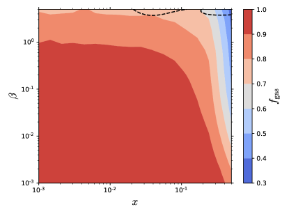
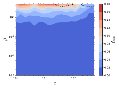
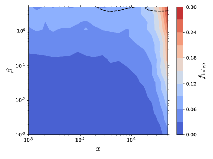
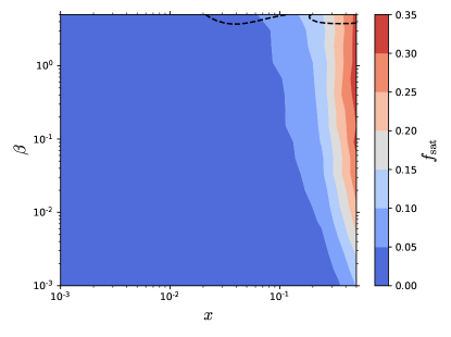
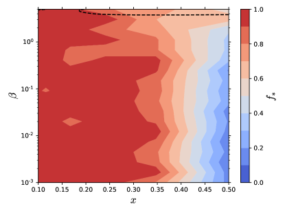
Figure 7: Results of the mirror structure formation analysis. The top four panels show the average fraction of mirror particles in each component of galactic structure (hot gas, disk, bulge and satellite galaxies) in a $10^{12}$ M_⊙ halo such that $f_{\mathrm{gas}}+f_{\mathrm{disk}}+f_{\mathrm{bulge}}+f_{\mathrm{sat}}=1$. The bottom panel shows the fraction of stars $f_{*}$ in the mirror galactic disk. The fraction of cold gas in the disk is given by $f_{\mathrm{cold}}=1-f_{*}$. The regions above the dashed curves are excluded from our analysis due to the self-consistency check discussed in section III.2.

The results of our SM  structure formation analysis are shown in figure 7, where the fractions of the different components $f_{\mathrm{gas}}$, $f_{\mathrm{disk}}$, $f_{\mathrm{bulge}}$, $f_{\mathrm{sat}}$ and $f_{*}$ (the fraction in stars in the disk) are plotted as functions of $(x,\beta)$. One of the most striking features is that for much of the parameter space ($x\lesssim 0.1$, $\beta\lesssim 1$), over 90 % of mirror matter is in a hot gas cloud and does not condense to form structures in the halo. This is readily understood, since the low density and low hydrogen abundance lead to inefficient cooling, maintaining high pressure in the gas cloud and preventing it from collapsing. Our results show that at low $x$ and in the range $0.5\lesssim\beta\lesssim 1$ about 5–10 % of the SM  forms a dark galaxy. In this case, even if the dark galaxy is subdominant in the halo, the mirror stars and supernovae within it would amplify the baryonic effects of SM particles, which have been argued to significantly alleviate the small-scale tension of CDM 2014ApJ…786…87B .

For SM  densities $\beta\lesssim 0.5$, mirror matter behaves similarly to generic models of dissipative DM, such as atomic DM, that have no nuclear or chemical reactions and do not collapse into compact objects. Although the SM  would constitute only a small fraction of DM and would not lead to dark stuctures (stars, planets, life forms), its dissipative effects could still have interesting cosmological effects, like the suppression of the matter power spectrum on small scales. The mirror gas cloud would also have a cored density profile, resulting in a shallower gravitational potential in the center of the halo than in a pure CDM scenario, possibly ameliorating the cusp-core problem.

The disk fraction $f_{\mathrm{disk}}$ depends much more strongly on $\beta$ than on $x$. This comes about because the long lifetime of the main halo allows for the formation of a mirror galaxy at sufficiently high density, even though cooling is less efficient at small $x$ (due to the low hydrogen fraction). The fraction $f_{\mathrm{sat}}$ of mirror matter in satellite galaxies behaves differently: even at large mirror particles densities, for $x<0.1$ the cooling timescale becomes longer than the lifetime of subhalos merging with the MW, leaving too little time for structures to form. Hence dwarf galaxies orbiting the MW will host few mirror particles if $x<0.1$. It is likely however that we underestimate $f_{\mathrm{sat}}$ due to our assumption that galaxy formation ended once the subhalos merged with the main halo. In reality the satellite galaxies can accrete cooling gas from the main halo and continue to grow after a merger.

There is a clear correlation between $f_{\mathrm{bulge}}$ and the sum of $f_{\mathrm{disk}}$ and $f_{\mathrm{sat}}$, which arises because bulge formation requires both the main halo and the satellite subhalos to form, before the latter is disrupted by dynamical friction. The absence of a disk for $x\gtrsim 0.1$, where $f_{\mathrm{bulge}}$ is at its maximum, indicates that a major merger destroyed the disk of the central halo. That major merger is probably recent, otherwise the disk would have had time to form again. Similarly, we can understand the small bulge fraction in the region $\beta\gtrsim 0.2$, $x\lesssim 0.1$ as resulting from a series of minor mergers or an early-time major merger, since there is a significant disk fraction at $z=0$ for these parameters.

The bottom panel of fig. 7 shows the effect of the shortened stellar lifetime in the SM  (see eqs. (III.4) and (53)). The high He abundance and the larger mass of primordial stars increase the stellar feedback from supernovae to a point where most of the cold molecular clouds are rapidly heated and return to the hot fraction of the halo, leaving mirror stars as the only inhabitants of the mirror galaxy.

Next we consider various astronomical constraints on SM  galactic structures. The excluded regions lie above the curves shown in fig. 8. The limits on disk surface density, bulge and total stellar mass, and from gravitational lensing surveys, are described in the following.

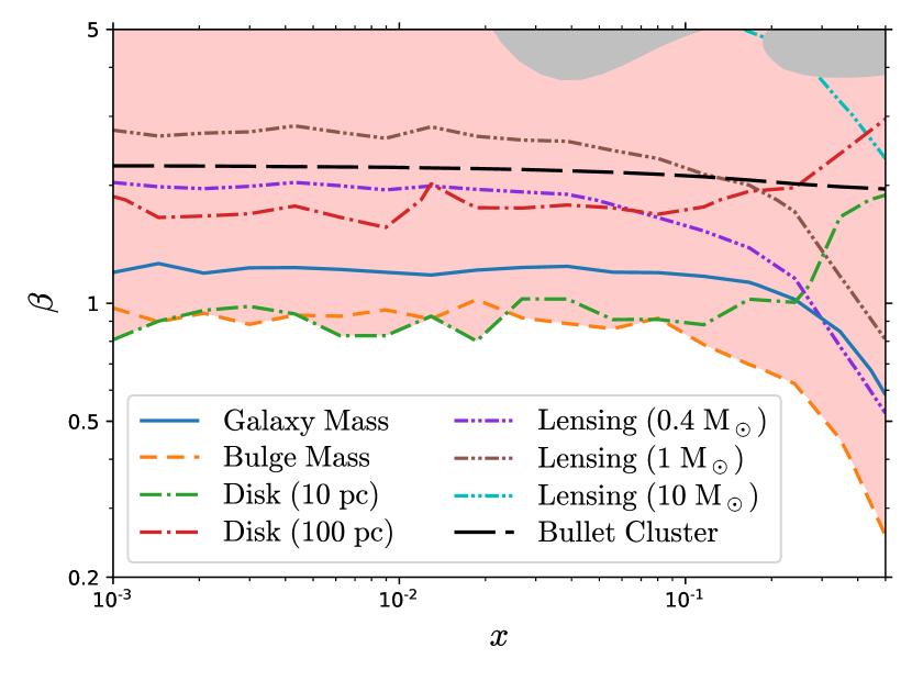
Figure 8: Upper limits for

SM

 model from constraints on: the total mass of the galaxy (defined as bulge plus disk, solid curve); the bulge mass (dashed); the thin disk surface density (dot-dashed), assuming $h_{D}=10$ (green) or 100 pc (red) for the dark disk; gravitational lensing events (double-dot-dashed) for $m_{\mathrm{mac}}=0.4$ (violet), 1 (brown) or 10 (cyan) M_⊙; and the Bullet Cluster (long-dashed). The red shaded area is excluded, while the grey regions lie outside the validity of our analysis (see section III.2).

IV.1 Thin disk surface density

Data from Gaia DR2 allowed ref. Buch:2018qdr to constrain the surface density $\Sigma_{D}$ of a thin dark disk in the vicinity of the Sun. A gravitational potential in the presence of a DM disk would be deeper, leading to greater acceleration towards the galactic plane than what ordinary stars can account for. This affects the transverse velocities and density distribution of nearby stars. Assuming that the dark disk possesses an exponential profile and a scale height $h_{D}\simeq 10$ pc (which could explain phenomena like the periodicity of comet impacts r2014dark ; schutz2017constraining ), the 95 % C.L. bound on its local surface density is

$$\Sigma_{D}(R_{\odot})=\frac{M_{D}}{2\pi L_{D}^{2}}e^{-R_{\odot}/L_{D}}\lesssim 4.15\ {\text{M}_{\odot}\over\text{pc}^{2}},$$ (56)

where $R_{\odot}=8.1$ kpc is the distance of the Sun from the center of the galaxy and $L_{D}$ is the scale length of the disk. The scale length is related to the half-mass radius $r_{D}$, which we included in our analysis, as $r_{D}/L_{D}\simeq 1.68$.

The constraint (56) led ref. Buch:2018qdr to conclude that a dissipative dark sector can constitute less than 1 % of the total DM. However a more conservative interpretation is that less than 1 % of the DM has accreted into a thin dark disk; in that case the dissipative dark sector could be more abundant since we expect only a fraction of it to form a galactic disk, $\lesssim 20\leavevmode\nobreak\ \%$ for mirror matter, as shown in fig.  7.

Assuming a thin disk with scale height $h_{D}=10$ pc, this bound rules out the region $\beta\gtrsim 1$, except for $x\gtrsim 0.25$ where it is relaxed to $\beta\gtrsim 1.8$. For a thicker disk with $h_{D}=100$ pc, closer to the height of the visible disk, the constraint is relaxed to $\Sigma_{D}(R_{\odot})\lesssim 12.9\ \text{M}_{\odot}/\text{pc}^{2}$, loosening the bound on $\beta$ by a factor of $\sim 2$.

An underlying assumption is that the dark disk lies withing the MW plane. Although the two disks need not be initially aligned, one expects their gravitational attraction to do so on the dynamical timescale of the inner region of the halo, $t_{\mathrm{dyn}}\sim 1/\sqrt{G\rho}\sim\sqrt{L_{D}^{3}/GM_{D}}$. Even if the dark disk has a negligible density such that only the visible disk contributes to $t_{\mathrm{dyn}}$ ($M_{D}\sim 10^{10}$ M_⊙, $L_{D}\sim 2.5$ kpc), one finds $t_{\mathrm{dyn}}\sim 20$ Myr, much shorter than the lifetime of the halo. Hence in all cases the two disks should be coincident.

IV.2 Bulge and total stellar mass

Data from Gaia DR2 further enabled ref. cautun2019milky to determine the total mass of each component of the MW halo by fitting the rotation curves of nearby stars and using other kinematical data. They determined the mass of the galaxy (disk and bulge components combined) to be $4.99^{+0.34}_{-0.50}\times 10^{10}$ M_⊙ in a $1.12\times 10^{12}$ M_⊙ halo. Scaling down their result to coincide with our $10^{12}$ M_⊙ halo, the total mass of the galactic components in our simulation should be $M_{\mathrm{gal}}=4.46^{+0.30}_{-0.45}\times 10^{10}$ M_⊙.

Since this measurement was obtained from stellar dynamics only, it is sensitive to the presence of a mirror galactic component. However it is difficult to accurately estimate the contribution of ordinary baryons to the disk + bulge mass from the mass-luminosity relation. It is believed that about 20 % of the baryons in the halo should condense into compact structures in the galaxy (see behroozi2010comprehensive and references therein), which represents a visible matter contribution of $3.1\times 10^{10}$ M_⊙. This leaves room for the remainder to come from a mirror galaxy component.

Under this assumption, we derive a $2\,\sigma$ upper bound on the mass of the mirror galaxy (disk + bulge),

$$M_{\mathrm{gal}}^{\prime}\lesssim 2\times 10^{10}\ \mathrm{M}_{\odot}.$$ (57)

It is also possible to constrain the bulge mass of the MW separately. Ref. cautun2019milky determined $M_{\mathrm{bulge}}=0.93^{+0.9}_{-0.8}\times 10^{10}$ M_⊙ using Gaia DR2, in agreement with the value of ref. sofue2013rotation obtained from rotation curves. A larger value was derived using photometric data from the VVV survey, estimating the contribution from visible stars to the bulge mass as $M_{\mathrm{bulge}}^{\mathrm{SM}}=2.0\pm 0.3\times 10^{10}$ M_⊙ portail2015madetomeasure ; zoccali2018weighing . Combining errors in quadrature, these imply the $2\,\sigma$ upper bound on the SM  contribution

$$M_{\mathrm{bulge}}^{\prime}=M_{\mathrm{bulge}}-M_{\mathrm{bulge}}^{\mathrm{SM}}\lesssim 0.83\times 10^{10}\ \mathrm{M}_{\odot}\,.$$ (58)

Both (57) and (58) imply limits comparable to that from the dark disk surface density, excluding $\beta\gtrsim 1$ for any $x$. Due to the increased bulge fraction at large $x$, the bound on $M_{\mathrm{bulge}}^{\prime}$ becomes tighter at large $x$, ruling out $\beta\gtrsim 0.3$ at $x\simeq 0.5$.

IV.3 Gravitational lensing

Compact objects made of mirror matter could be detected through their gravitational lensing of distant stars, similar to more general “MACHO” models of DM. However, it is difficult to predict the microlensing rate from SM  structures since it depends strongly on their masses. Like in the SM, these compact objects could include asteroids and comets, planets, molecular clouds, or stars and dense globular clusters, spanning over 15 orders of magnitude in mass. We will focus on compact objects of mass $10^{-1}$ M${}_{\odot}\lesssim M\lesssim 10$ M_⊙, corresponding to a main-sequence star or a small molecular cloud. As in the SM, smaller objects should represent a negligible fraction of the collapsed matter in the SM .

Constraints on the MACHO fraction $f_{\mathrm{mac}}$ of DM in this mass range have been discrepant. The MACHO collaboration studied microlensing events towards the Large Magellanic Cloud (LMC) and initially reported evidence that MACHOs of mass $(0.15-0.9)$ M_⊙ comprise (8-50) % of the total halo DM Alcock:2000ph , but it was later found that their dataset was contaminated by variable stars Bennett:2005at . The same survey showed no evidence for MACHOs in the mass range ($0.3-30$) M_⊙ Allsman:2000kg . The EROS and OGLE surveys found no evidence for MACHOs towards the LMC wyrzykowski2010ogle ; wyrzykowski2009ogle ; Tisserand:2006zx ; 1997A&A…324L..69R leading them to place an upper limit $f_{\mathrm{mac}}\lesssim(7-30)$ %. The MEGA and POINT-AGAPE experiments came to different conclusions, the former finding no evidence for MACHOs towards M31 deJong:2005jm while the latter reported $0.2\lesssim f_{\mathrm{mac}}\lesssim 0.9$ CalchiNovati:2005cd .

To interpret these results we review some of the theory underlying MACHO searches. Gravitational lensing is characterized by an optical depth

$$\tau=\frac{4\pi GD_{s}^{2}}{c^{2}}\int_{0}^{1}\rho(x)\,x(1-x)\,dx,$$ (59)

where $D_{s}$ is the distance to the amplified star and the integral is taken along the line of sight, with $x$ in units of $D_{s}$. The optical depth is the instantaneous probability that a star’s brightness is amplified by a factor of at least $1.34$, and is proportional to the mass density $\rho$ of the lens.

If $N_{\mathrm{s}}$ stars are monitored during a period $T_{\mathrm{obs}}$, then the expected number of detected microlensing events is

$$N_{\mathrm{ex}}=\frac{2}{\pi}\frac{T_{\mathrm{obs}}}{\langle t_{E}\rangle}\tau N_{\mathrm{s}}\langle\epsilon\rangle,$$ (60)

where $\langle t_{E}\rangle$ is the average Einstein radius crossing time and $\langle\epsilon\rangle$ is an efficiency coefficient that depends on the experimental selection criteria.

All the constraints cited above assumed that the MACHOs have an isothermal density profile $\rho\sim(r^{2}+r_{0}^{2})^{-1}$, which is often referred to as the “S model.”   This assumption is not valid for mirror matter compact objects since they are preferentially distributed in the disk and the bulge of galaxies, like visible stars. Ref. Alcock:2000ph estimated the total optical depth due to visible stars in the MW and the LMC galaxies as $\tau\simeq 2.4\times 10^{-8}$ with an average Einstein radius crossing time $\langle t_{E}\rangle\simeq 60$ days.

The optical depth $\tau^{\prime}$ due to a mirror galaxy is roughly proportional to its mass; we can therefore estimate it as $\tau^{\prime}\simeq\tau\beta\times(f_{\mathrm{mac}}/0.2)$, where $f_{\mathrm{mac}}=f_{\mathrm{disk}}+f_{\mathrm{bulge}}+f_{\mathrm{sat}}$ is the fraction of mirror particles that form compact objects in both the MW and its satellite galaxies. The factor of $0.2$ comes from the estimate that $\sim 20$ % of the SM baryons in the halo end up in stars. In reality the contribution from each component weighs differently in the value of $\tau$: MACHOs in the LMC are about twice as likely to produce a lensing event as one located in the MW bulge or disk. To be more precise we should sum the optical depth $\tau_{i}^{\prime}\simeq\tau_{i}(M_{i}^{\prime}/M_{i})$ of each component, where $M_{i}$ ($M_{i}^{\prime}$) is the mass of ordinary (mirror) stars in the LMC or in the MW bulge or disk. But the stellar masses of the LMC and of the individual MW components have large uncertainties and our simple treatment of satellite galaxies does not allow for an accurate identification of an LMC-like subhalo and the mass of its mirror galaxy. We can nevertheless make an order-of-magnitude estimate of $\tau^{\prime}$ by putting all contributions on an equal footing and using the global fraction $f_{\mathrm{mac}}$ of condensed objects in the halo.

Since the Einstein radius is proportional to the square root of the mass of the lens Tisserand:2006zx , the value of $\langle t_{E}\rangle$ can also be different in the SM . Assuming a fiducial mass of $0.4\,M_{\odot}$ for SM stars, then we can approximate $\langle t_{E}^{\prime}\rangle=\langle t_{E}\rangle\sqrt{m_{\mathrm{mac}}/0.4\,M_{\odot}}$, where $m_{\mathrm{mac}}$ is the mirror MACHO mass.

The EROS-2 survey sets one of the most stringent limit on MACHOs in the direction of the LMC. During $T_{\mathrm{obs}}=2500$ days, it monitored $N_{\mathrm{s}}=5.5\times 10^{6}$ stars and detected no microlensing event. This sets the 95 % confidence limit $N_{\mathrm{ex}}<3$. From visible stars alone we expect $N_{\mathrm{ex}}\simeq 1.23$ events for an efficiency coefficient $\langle\epsilon\rangle\approx 0.35$. Then the limit on events from mirror stars is $N_{\mathrm{ex}}^{\prime}\lesssim 1.77$, giving

$$\beta f_{\mathrm{mac}}\lesssim 0.29\left(\frac{0.35}{\langle\epsilon^{\prime}\rangle}\right)\sqrt{\frac{m_{\mathrm{mac}}}{0.4M_{\odot}}}\,,$$ (61)

where $\langle\epsilon^{\prime}\rangle$ is the efficiency coefficient of the SM , which could differ from the SM value if the MACHO mass is different. We will consider three benchmark values of $m_{\mathrm{mac}}$ to constrain our model: 0.4 M_⊙, 1 M_⊙ and 10 M_⊙. For simplicity we will also assume $\langle\epsilon^{\prime}\rangle\approx 0.35$ for all masses.

The constraint (61) is not very restrictive, despite mirror matter being capable of forming roughly as many compact objects as visible matter. If mirror stars had a mass distribution similar to visible stars, then $m_{\mathrm{mac}}\simeq 0.4$ M_⊙ would only rule out $\beta\gtrsim 2$, which is already excluded by other observations. It is possible that the typical SM  MACHO mass exceeds that of SM stars since cooling and cloud fragmentation are less efficient in the SM , as we argued in section III.4. In that case the bound would be relaxed even more. A full analysis of the stellar evolution in the SM , including heavier elements that we have not included, would be required to estimate $m_{\mathrm{mac}}$ and the microlensing rate more accurately. But based on the present analysis, it seems unlikely that MACHO detection towards the LMC could be more constraining than the disk surface density or the stellar mass in the MW.

IV.4 Bullet Cluster

Interestingly, the Bullet Cluster allows us to set an upper limit on the hot gas fraction of mirror baryons, i.e., the absence of structure formation in the SM . The visible galaxies and stars on the scale of this cluster are essentially collisionless, but the hot gaseous baryons that surround the galaxies were impeded by dynamical friction and stripped from their hosts. Similarly, mirror galaxies and stars pass through each other unimpeded, just like CDM, while the hot clouds of mirror baryons will self-interact.

The most stringent constraint on DM comes from the survival of the smaller subcluster in the merger, as less than 30 % of its mass inside a radius of 150 kpc was stripped in the collision Markevitch:2003at . This normally yields a bound on the integrated cross section $\sigma/m$. Here we instead follow the approach of ref. Foot:2014mia , constraining the distribution of mirror matter, in particular the mass of the hot gas fraction. We recapitulate the argument as follows.

Consider the elastic collision of two equal-mass mirror particles in the subcluster’s reference frame. The incoming particles from the main cluster have an initial velocity $v_{0}\approx 4800$ km/s. After the collision, they scatter with velocities

$$v_{1}=v_{0}\cos\Theta,\quad v_{2}=v_{0}\sin\Theta,$$ (62)

where $\Theta$ is the scattering angle of the incoming particle in the subcluster’s frame.

For the subcluster to lose mass, both particles must be ejected from the halo: $v_{1},v_{2}>v_{\rm esc}$ where $v_{\rm esc}\approx 1200$ km/s is the escape velocity. This happens for a scattering angle $\theta$ (in the CM frame)

$$\frac{v_{\rm esc}}{v_{0}}<\sin\frac{\theta}{2}<\sqrt{1-\left(\frac{v_{\rm esc}}{v_{0}}\right)^{2}}.$$ (63)

The scattering angles in the two frames are related by $\Theta=\theta/2$ for equal-mass particles. The evaporation rate is $R=N^{-1}dN/dt$ where $N$ is the total number of hot mirror particles in the subcluster. It can be expressed as Kahlhoefer:2013dca

$$R=n_{2}v_{0}\int_{\rm esc}\frac{d\sigma}{d\Omega_{CM}}d\Omega_{CM},$$ (64)

where $n_{2}$ is the number density of mirror particles in the main cluster and the bounds of the integral are given by eq. (63). Integrating (64) over the crossing time $t=w/v_{0}$, where $w$ is the width of the main cluster, leads to the fraction of evaporated hot mirror particles,

$$\frac{\Delta N}{N}=1-\exp\left(-\frac{\Sigma_{2}}{\overline{m_{N}}}\int_{esc}\frac{d\sigma}{d\Omega_{CM}}d\Omega_{CM}\right),$$ (65)

where $\Sigma_{2}$ is the surface density of the hot mirror matter gas in the main cluster. Taking the total DM surface density to be $\Sigma_{\mathrm{DM}}\simeq 0.3$ g/cm², we can estimate $\Sigma_{2}\simeq f_{\mathrm{gas}}^{\mathrm{BC}}(\Omega_{b^{\prime}}/\Omega_{\mathrm{DM}})\Sigma_{\mathrm{DM}}$, where $f_{\mathrm{gas}}^{\mathrm{BC}}$ is the hot mirror matter gas fraction in the main cluster.

Because of the large mass of the cluster and the subcluster ($M\gtrsim 2\times 10^{14}\,M_{\odot}$), the virial temperature of the mirror matter gas is high enough to fully ionize the H and He atoms. Mass evaporation therefore proceeds via Rutherford scattering between ions. Assuming that all mirror nuclei have a mass $\overline{m_{N}}$ and a charge $Z=1+f_{\mathrm{He}}$ (see eqs. (6,7)), their differential cross section in the CM frame is

$$\frac{d\sigma}{d\Omega_{CM}}=\left(\frac{Z^{2}\alpha}{4E\sin^{2}(\theta/2)}\right)^{2}.$$ (66)

where $E=\overline{m_{N}}(v_{0}/2)^{2}$ is the total kinetic energy in the CM frame. Plugging this in eq. (65) and evaluating the integral within the bounds of eq. (63) yields

$$\frac{\Delta N}{N}=1- \exp\bigg{\{}\frac{-4\pi Z^{4}\alpha^{2}\Sigma_{2}}{\overline{m_{N}}^{3}v_{0}^{4}}$$ (67)

$$\times\frac{1-2\left(v_{esc}/v_{0}\right)^{2}}{\left(v_{esc}/v_{0}\right)^{2}\left(1-\left(v_{esc}/v_{0}\right)^{2}\right)}\bigg{\}}.$$

Assuming that only hot mirror particles are stripped in the collision, the constraint on the evaporated mass fraction of the subcluster is:

$$f_{\mathrm{evap}}=\frac{f_{\mathrm{gas}}^{\mathrm{BC}}\beta\Omega_{b}}{\Omega_{\mathrm{DM}}}\frac{\Delta N}{N}<0.3.$$ (68)

This does not apply directly to our study, since we specifically studied structure formation in a $10^{12}$ M_⊙ halo, while the Bullet subcluster has mass $\sim 2\times 10^{14}$ M_⊙. However ref. behroozi2010comprehensive indicates that the stellar mass fraction in a Bullet subcluster-sized halo is $\sim 10$ % of the same fraction in a MW-like halo. We can therefore estimate the hot gas fraction of SM  matter in the Bullet Cluster as $f_{\mathrm{gas}}^{\mathrm{BC}}\simeq(1-0.1)f_{\mathrm{mac}}$ (recall that $f_{\mathrm{mac}}$ is the fraction of mirror matter compact objects in the central galaxy and its satellites, that we derived above). However this is weaker than the kinematic data limits, and the resulting bound from the Bullet Cluster is similar in strength to that from microlensing, excluding only the region $\beta\gtrsim 2$.

IV.5 Future constraints and signals

In this section we describe other astronomical observations that could lead to new constraints on the SM  in the next few years, as more data is collected and experimental sensitivity increases.

Gravitational wave (GW) astronomy is a promising new window to study our universe and the properties of DM. LIGO and other interferometer experiments are forecasted to put strong constraints on the fraction of primordial black holes (PBHs) in the universe, down to a mass scale of $\sim 10^{-13}$ M_⊙ Saito:2008jc ; saito2009gravitationalwave ; Carr:2009jm ; Carr:2016drx . However, the binary black hole (BBH) merger rate $\mathcal{R}_{BBH}^{exp}\sim 9.7-101$ Gpc^-3 y^-1 detected by LIGO LIGOScientific:2018mvr seems to exceed the predictions of $\mathcal{R}_{BBH}^{th}\sim 5.4$ Gpc^-3 y^-1 in some theoretical models of star formation Askar:2016jwt .

In has been suggested in Beradze:2019dzc ; Beradze:2019ujd that this discrepancy could be explained by the early formation of BHs in mirror matter-dominated systems. This idea is supported by the fact that none of the GW signals from BBH mergers detected by LIGO were accompanied by an electromagnetic counterpart, indicating that those systems had accreted very little visible matter. A similar idea can be applied to binary neutron star (NS) mergers and BH-NS coalescence Beradze:2019yyp , which only led to the detection of one electromagnetic signal Cowperthwaite:2017dyu out of the many candidate events.

According to Beradze:2019dzc ; Beradze:2019ujd , since the cosmic star formation rate (SFR) peaked at $z\sim 1.9$ for visible matter, then it should have peaked at a redshift $z^{\prime}\simeq-1+(1+1.9)/x$ in the SM , leaving more time for mirror matter to form BHs and binary systems. According to our present findings, this argument is incorrect, since we have shown that star formation depends primarily on chemical abundances, matter temperature and the gravitational potential, not on the background radiation temperature. At late times ($z\ll z_{\rm dec}$), visible and mirror particles collapse inside the same local gravitational potential well and they are shock-heated to the same temperature $\sim T_{\mathrm{vir}}$ (recall eq. (36)). Hence the mirror SFR differs from that of the SM only because of its high He abundance and how it impacts the cooling rate. These effects are not encoded by a simple $x$-dependent rescaling of $z$.

Nevertheless, the authors of DAmico:2017lqj ; Latif:2018kqv suggested that the inefficient cooling and fragmentation of mirror gas clouds could lead to the early formation of direct collapse black holes (DCBHs). Although they would more likely act as supermassive BH seeds, they could also increase the binary merger rate in the mass range probed by LIGO and the other GW interferometers. In the next decade, as the measurements and predictions for $\mathcal{R}_{BBH}$ are refined, as well as the understanding of BH formation from mirror matter, this could be a useful observable to further constrain such models.

21-cm line surveys are another promising technique for studying late-time cosmology and structure formation. The EDGES experiment reported a surprisingly deep absorption feature in the signal emitted at the epoch of reionization Bowman:2018yin . Although it still awaits confirmation, many have tried to relate this anomaly to DM properties Munoz:2018pzp ; Fialkov:2018xre ; Berlin:2018sjs ; Barkana:2018cct ; Liu:2019knx ; Panci:2019zuu . Mirror matter could be compatible with the EDGES result if the model is augmented by a large photon-mirror photon kinetic mixing term, $\epsilon\sim 10^{-3}$, and if the CDM is light, $\sim 10$ MeV. To explain the EDGES anomaly would also require breaking the mirror symmetry by allowing for a new long-range force between the DM and the CDM, as shown in ref. Liu:2019knx . (The large kinetic mixing would evade constraints from underground direct detection since millicharged mirror DM would not be able to penetrate the earth.) Ref. AristizabalSierra:2018emu proposed an alternative mechanism in which mirror neutrinos decay to visible photons, $\nu_{i}^{\prime}\to\gamma\nu_{j}$, to explain the EDGES anomaly, using a smaller kinetic mixing $\epsilon\lesssim 10^{-6}$. This scenario too would require mirror symmetry breaking, in the form of a small SM  photon mass. These two models might require even further breaking of the mirror symmetry in order to avoid stringent limits $\epsilon\lesssim 10^{-9}-10^{-7}$ set by $N_{\rm eff}$ Foot:2014mia ; Berezhiani:2008gi and orthopositronium decay Vigo:2018xzc in the unbroken symmetry scenario.

Independently of whether the EDGES anomaly is confirmed, furture 21-cm line surveys can be used to constrain compact DM objects like mirror stars. Should mirror matter compact objects form before visible stars (as in the early formation of DCBHs proposed by DAmico:2017lqj ; Latif:2018kqv ), those objects would accrete visible matter and accelerate the reonization of the universe, leaving a characteristic imprint on the 21-cm signal Mena:2019nhm and distorting the CMB spectrum Ricotti:2007au . The suppression of the power spectrum by a dark sector, as we discussed in section III.2, is also expected to delay structure formation and the absorption feature of the 21-cm line Lopez-Honorez:2018ipk .

It was recently suggested that gravitational lensing of fast radio bursts would present a characteristic interference pattern and could probe MACHOs in the mass range $10^{-4}$ – $0.1$ M_⊙ Katz:2019qug . Although this is smaller than the typical mass scale for mirror stars, it could lead to new constraints on the abundance of smaller objects, like mirror brown dwarfs and mirror planets.

The idea that mirror planets could orbit visible stars (or the opposite) was proposed two decades ago Foot:1999ex ; Foot:2000iu , but not explored in detail. A smoking gun signal for small mirror matter structures would be the detection of an exoplanet-like object via Doppler spectroscopy or microlensing without the expected transit, in the case where the inclination angle is $90^{\circ}$. With improved understanding of how mirror planets form and how often they could be captured by a visible stars, the nondiscovery of such events could eventually rule out some of the parameter space of the model.

Finally, mirror stars would heat and potentially dissolve visible wide binary star systems, star clusters and ultra-faint dwarf galaxies via dynamical relaxation. This effect was used to rule out heavy MACHOs ($m\gtrsim 5-10\,M_{\odot}$) from making up a significant fraction of DM Brandt:2016aco ; 2010ASPC..435..453Q . Future studies of similar systems could tighten the constraints on MACHOs and, pending a more refined model for mirror star formation, on mirror matter.

V Early universe

One may wonder how likely it is to find an embedding of perfect mirror symmetry in a complete model including inflation and baryogenesis, such that the relative temperatures and baryon asymmetries in the two sectors differ as we have presumed. These questions have been considered in earlier literature. Here we revisit them in light of more recent inflationary constraints.

V.1 Temperature asymmetry

A simple way of maintaining mirror symmetry while incorporating cosmological inflation is to assume that each sector has its own inflaton, and to seek differences in their reheating temperatures from initial conditions or other environmental effects, while maintaining identical microphysics in each sector. An early proposal for getting asymmetric reheating was given in ref. 1985Natur.314..415K , which proposed a ‘double-bubble inflation’ model where the ordinary and mirror inflatons finish inflation by bubble nucleation at different (random) times. In this case the first sector to undergo reheating gets exponentially redshifted until the second field nucleates a bubble of true vacuum. However this is in the context of “old inflation” driven by false vacua, which is untenable because the phase transitions never complete.

A more promising mechanism was demonstrated in ref. Berezinsky:1999az , which considered two-field chaotic inflation with decoupled quadratic potentials, with total potential of the form

$$V_{\rm tot}=V(\phi)+V(\phi^{\prime})$$ (69)

plus respective couplings of each field to its own sector’s matter particles, to accomplish reheating. It was shown that the solutions are such that the ratio of the two inflatons $\phi^{\prime}/\phi$ remains constant during inflation. Then the ratio of the reheating temperatures goes as $(\phi^{\prime}/\phi)^{2/3}$, and is thereby determined by the random initial conditions. This idea is now ruled out by Planck data Akrami:2018odb , strongly disfavoring chaotic inflation models, that have concave potentials.

We suggest a possible way of saving this scenario; one can flatten the potentials at large field values using nonminimal kinetic terms Lee:2014spa , for example

$${\cal L}_{\rm kin}=\left(1+f{\phi^{4}\over m_{P}^{4}}\right)(\partial\phi)^{2}+\left(1+f{\phi^{\prime 4}\over m_{P}^{4}}\right)(\partial\phi^{\prime})^{2}$$ (70)

For $\phi,\phi^{\prime}\gg m_{P}$, the canonically normalized fields are $\chi\sim\phi^{3}$, $\chi^{\prime}\sim\phi^{\prime 3}$, so that a potential of the form $m^{2}(\phi^{2}+\phi^{\prime 2})$ becomes proportional to $(\chi^{2/3}+\chi^{\prime 2/3})$, mariginally consistent with Planck constraints on the tensor-to-scalar ratio and spectral index, while maintaining the separability of the potential. In common with the simpler model, the trajectory in field space is a straight line towards the vacuum at $\phi=\phi^{\prime}=0$ and the initial conditions determine the ratio of reheat temperatures, $x=T_{R}^{\prime}/T_{R}$. We leave this for future investigation.

Alternatively, one could imagine there is just a single inflaton, that is charged under the mirror symmetry such that $\phi\to-\phi$, and couples to the Higgs fields of the two sectors with opposite signs,

$$V\supset V_{\rm inf}(\phi)+\frac{\mu}{2}\phi\left(h^{\prime 2}-h^{2}\right)+V(h)+V(h^{\prime})$$ (71)

so as to preserve the mirror symmetry. At the end of inflation, $\phi$ oscillates about its minimum at $\phi=0$, resulting in a time-dependent frequency $\omega_{k}$ for the Fourier modes of the Higgs fields Dufaux:2006ee ,

$$\omega_{k}^{2}=m^{2}_{h}+\frac{k^{2}}{a^{2}}\pm\frac{\mu\Phi}{a^{3/2}}\sin(m_{\phi}t),$$ (72)

where $\Phi$ is the amplitude of the inflaton at the beginning of preheating. Both fields are periodically tachyonic whenever $\omega_{k}^{2}<0$, resulting in an exponential growth of the occupation number: $n_{k}\sim\prod_{j}\exp(X_{k}^{j})$, where $X^{j}_{k}$ is the particle production rate during the $j$th inflaton oscillation.

With the expansion of the universe, the particle production efficiency decreases: $X_{k}^{j}\sim a(t_{j})^{-3/4}$ Abolhasani:2009nb , where $a(t_{j})$ is the average scale factor during the $j$th tachyonic phase. Because of their opposite coupling to the inflaton, the tachyonic resonances of $h_{k}$ and $h^{\prime}_{k}$ are out of phase with each other, resulting in different growth rates. In particular, the first field to experience tachyonic instability gives rise to dominant reheating into its own sector, creating a temperature difference between the two. Details will be given in a future publication.

V.2 Baryogenesis

A further challenge is to explain how the SM  baryon asymmetry could attain values compatible with the allowed regions from our analysis. The baryon densities in the two sectors are related by

$$\eta_{b^{\prime}}={\beta\over x^{3}}\eta_{b}\,.$$ (73)

where $\eta_{b^{\prime}}=n_{b^{\prime}}/s^{\prime}$, with $s^{\prime}$ being the entropy density of the SM , while $\eta_{b}=n_{b}/s$, where $s$ is the SM entropy density. Hence for $\beta\sim 0.3$ and $x\sim 0.5$, for example, we require would baryogenesis in the SM  to be more efficient than in the SM: $\eta_{b^{\prime}}/\eta_{b}=2.4$. Lowering the value of $x$ with $\beta$ fixed requires an even greater efficiency for mirror baryogenesis.

Leptogenesis may offer a viable explanation for this mild hierarchy. Naively one could expect that $\beta\leavevmode\nobreak\ \simeq\leavevmode\nobreak\ x^{3}$ since this is the ratio of the densities of the decaying heavy neutrinos in the two sectors, which would lead to a very small mirror baryon abundance. In particular, if $x\lesssim 0.1$ mirror particles would be too sparse to produce any observable signal. However this assumes that the washout factor is the same in both sectors, which need not be the case. At any given time, mirror heavy neutrino decays occur farther out of equilibrium than those of their SM counterparts, due to their lower temperature (while the Hubble rate is the same for both sectors). This can make the washout factor smaller in the SM  Buchmuller:2004nz leading to more efficient leptogenesis in that sector. This conclusion is compatible with refs. 1985Natur.314..415K ; Berezhiani:2000gw , which considered the analogous mechanism of GUT baryogenesis, that also relies upon an asymmetry produced by out-of-equilibrium decays. They also found that $\beta\sim x^{3}$ for particles decaying well out of equilibrium, while $\beta\sim x$ in the strong washout regime. Hence for some intermediate choice it should be possible to have $x^{3}<\beta<x$ as in our example of $\beta\sim 0.3$ and $x\sim 0.5$. In general these scenarios predict that baryogenesis in the SM  is at least as efficient as in the SM, $\eta_{b^{\prime}}/\eta_{b}\geq 1$.

Ref. Berezhiani:2000gw in addition considered electroweak baryogenesis in the SM , and finds that $\beta=x^{3}$ is predicted for the typical case in which the phase transition is strong enough so that sphalerons are highly suppressed inside the bubbles of true electroweak vacuum. For finely tuned scenarios in which sphalerons washout is important for attaining the final baryon asymmetry, larger values of $\beta$ could achieved, since the phase transitions happens earlier in the SM sector, and thus gives longer time for sphalerons to washout the initial asymmetry.

V.3 Non-minimal mirror matter model

Although it goes beyond the scope of the present investigation, it is interesting to contemplate less minimal scenarios in which mirror symmetry is not exactly conserved at the microscopic level. This of course makes it easier to achieve the asymmetry between temperatures of the two sectors.

A simple example is to allow for the mirror Higgs field to have a different VEV, $v^{\prime}\neq v$, which changes the mirror fermions masses by the factor $v^{\prime}/v$. If $v^{\prime}/v>1$ and we introduce portal interactions between the two sectors in the early universe, there would be a net transfer of entropy to the less massive SM fermions until the two sectors decouple from each other and their temperature ratio freezes out. If mirror symmetry is already broken during reheating, it could affect the decay rate of the inflaton into each sector, leading to different reheating temperatures without portal interactions Berezhiani:1995am . Other mechanisms for the broken mirror parity scenario can be adapted from similar theories like twin Higgs models (see Chacko:2018vss and references therein). By generalizing the chemical and cooling rates described in Appendices A and B for the nonsymmetric SM , our present analysis could be repeated to study structure formation in this altered scenario.

Another variation of the model, already alluded to in section IV.5 is the inclusion of the Higgs portal interaction $h^{2}h^{\prime 2}$ or kinetic mixing $F^{\mu\nu}F^{\prime}_{\mu\nu}$ between the SM  and the SM. Although they are significantly constrained by laboratory and astrophysical considerations, they could still have important implications for cosmology and structure formation. In particular, ref. Foot:2014mia argued that mirror photons produced in ordinary supernovae would heat the dark SM  disk, leading to its expansion. Conversely, visible photons could be produced in early mirror supernovae and accelerate the reionization of ordinary baryons Foot:2004kd . These portal interactions would also open the possibility for direct detection experiments and give characteristic astronomical signals Curtin:2019ngc .

VI Conclusions

Working within the context of unbroken mirror symmetry, we have investigated the formation of dark galactic structures of mirror matter in a MW-like halo and constrained the parameters $x=T^{\prime}/T$, $\beta=\Omega_{b^{\prime}}/\Omega_{b}$ of the theory using astrophysical data. By our assumption, all chemical and nuclear processes have the same rates in each sector, but mirror baryons turn out to be He-dominated because of their lower temperature.

The lower temperature and large He abundance of the SM  have many consequences for its cosmology and structure formation. H and He recombination are generally more efficient, leaving a lower density of free electrons at late times. While H₂ formation is also more efficient in the SM , its residual density is suppressed by the low H abundance. H₂ and free electrons are the two main cooling channels of hot gas clouds in the SM; their low abundances in the SM  imply that cooling and fragmentation of mirror gas clouds are less efficient, which alters structure formation. We find that primordial mirror stars are much more massive than their visible counterparts. Because of the He fraction, the lifetime of mirror stars is drastically shortened, which in turns increases the SN feedback on collapsing gas clouds in the SM .

Overall, the formation of mirror galaxies is strongly inhibited for $\beta\lesssim 0.5$ and $x\lesssim 0.1$. For such parameters, mirror baryons tend to stay in an isothermal hot gas cloud, avoiding constraints from astronomical and cosmological data, making such a scenario difficult to distinguish from more generic models containing a subdominant component of dissipative dark matter. The most stringent such constraints come from observations of the MW disk surface density and bulge mass, which rule out $\beta\gtrsim 0.3$ at $x=0.5$ and $\beta\gtrsim 0.8$ for $x\lesssim 0.1$. Both of these are derived by comparing stellar kinematics (measured e.g. by Gaia) with spectroscopy data. One can therefore hope that the release of Gaia EDR3 in 2020 and improved understanding of luminosity data will shed more light on the existence of dark galactic structures. 21-cm line surveys and gravitational wave astronomy are also promising leads to explore the properties of DM.

It is theoretically challenging to generate a temperature asymmetry between the mirror and visible particles while maintaining unbroken mirror symmetry at the microscopic level. We proposed several ideas that could give rise to asymmetric reheating, which intuitively are expected to produce only a small hierarchy with $x\gtrsim 0.1$. Coincidentally this is the most constrained region of the model, hence the most interesting from the perspective of discovery.

Acknowledgment. We thank A. Benson, A. Ghalsasi, M. McQuinn and A. Lupi for very helpful correspondence. Our work is supported by NSERC (Natural Sciences and Engineering Research Council, Canada). JSR is also supported by the FRQNT (Fonds de recherche du Québec – Nature et technologies, Canada).

Appendix A Recombination evolution equations

Here we define quantities appearing in the evolution equations (10-12) that are needed for recombination in the mirror sector.

The Thomson scattering cross section is $\sigma_{T}$ is and $a_{R}=4\sigma/c$ is the radiation constant, related to the Stefan-Boltzmann constant $\sigma$. The other parameters come from the atomic configuration of both elements. The H⁰ 2s-1s frequency is $\nu_{\mathrm{H}}=2466.0$ THz, the He⁰ 2¹s-1¹s frequency is $\nu_{\mathrm{He}}=4984.9$ THz and $\tilde{\nu}_{\mathrm{He}}=145.62$ THz is the frequency difference between the 2¹p-1¹s and the 2¹s-1¹s transitions of He⁰. The two-photon rates are $\Lambda_{\mathrm{H}}=8.22458$ s^-1 and $\Lambda_{\mathrm{He}}=51.3$ s^-1.

The two recombination parameters $\alpha_{i}$ are given by (in m³ s^-1):

$$\alpha_{\mathrm{H}}=\frac{F}{10^{19}}\frac{at^{b}}{1+ct^{d}},$$ (74)

$$\alpha_{\mathrm{He}}=q\left[\sqrt{\frac{T_{M}^{\prime}}{T_{2}}}\left(1+\sqrt{\frac{T_{M}^{\prime}}{T_{2}}}\right)^{1-p}\left(1+\sqrt{\frac{T_{M}^{\prime}}{T_{1}}}\right)^{1+p}\right]^{-1},$$ (75)

where the fit coefficients are $a=4.309$, $b=-0.6166$, $c=0.6703$, $d=0.5300$ and $t=T_{M}^{\prime}/10^{4}$ K. $F$ is a fudge factor set to 1.125 Giesen:2012rp . Furthermore, $q=10^{-16.744}$, $p=0.711$, $T_{1}=10^{5.114}$ K and $T_{2}$ was fixed at 3 K. The principle of detailed balance gives the photoionization coefficients $\beta_{i}$:

$$\beta_{i}=g_{i}\alpha_{i}\left(\frac{m_{e}kT_{M}^{\prime}}{2\pi\hbar^{2}}\right)^{3/2}e^{-\chi_{i}/kT_{M}^{\prime}}.$$ (76)

The statistical weight factor $g_{i}$ is 1 for H and 4 for He and the ionization energies from the 2s level are $\chi_{\mathrm{H}}=3.3996$ eV and $\chi_{\mathrm{He}}=3.9716$ eV.

Finally, the coefficients $K_{i}$ take into account the cosmological redshift of the H Ly$\alpha$ and He⁰ 2¹p-1¹s photons that reionize the atoms. They are given by $K_{i}=\lambda_{i}^{3}/(8\pi H(z))$ with $\lambda_{\mathrm{H}}=121.5682$ nm and $\lambda_{\mathrm{He}}=58.4334$ nm.

Appendix B Cooling rates and chemical abundances

Here we describe the various processes that contribute to the cooling of dark baryons, and their rates.

(i) Inverse Compton scattering. At early times, electrons can exchange energy with the background photons, with cooling rate

$$\mathcal{C}_{\mathrm{Comp}}=\frac{4T_{M}}{m_{e}}\sigma_{T}n_{e}a_{R}T^{4}.$$ (77)

where $T_{M}$ is the matter temperature (given by eq. 36) and $T$ is the radiation temperature. Because the expansion of the universe redshifts $T$, inverse Compton cooling becomes negligible at late times.

(ii) Brehmsstrahlung. At very high temperatures the gas will be fully ionized and will primarily cool via free-free emissions (bremsstrahlung), whose cooling rate is:

$$\mathcal{C}_{\mathrm{ff}}=\frac{16\alpha^{3}g_{\mathrm{ff}}}{3}\left(\frac{2\pi T}{3m_{e}^{3}}\right)^{1/2}n_{e}\sum_{\mathrm{ions}}n_{i}Z_{i}^{2}.$$ (78)

The sum runs over the ionized species (H⁺, He⁺ and He⁺⁺) and $Z_{i}$ is their electric charge. For our analysis we took the Gaunt factor to be $g_{\mathrm{ff}}\simeq 1$.

(iii) Atomic transitions. When the ionization fraction of the gas is too small, bremsstrahlung becomes inefficient. At this point atomic processes take the lead in the cooling of the gas. As ions and free electrons recombine to form neutral atoms, they radiate energy. Atoms can also collide with free electrons which will temporarily excite or ionize the atom until they return to their ground state. The atomic cooling rates $\mathcal{C}_{\mathrm{atom}}$ are given in table B.1.

(iv) Molecular transitions. Atomic cooling can only bring the gas to a temperature of $\sim 10\,000$ K (about 1 eV), since below this point electrons don’t carry enough energy to excite or ionize the atoms. But unlike atoms, molecular hydrogen possesses rotational and vibrational modes which are easily excited by collisions. As the molecules return to their ground state, they emit low-energy photons which allow the temperature to drop to $\sim 200$ K if H₂ is sufficiently abundant.

The cooling function for molecular hydrogen can be parametrized as follows 1979ApJS…41..555H ; Grassi:2013lha ; Glover:2008pz :

$$\mathcal{C}_{\mathrm{mol}}=\frac{n_{\mathrm{H_{2}}}L_{\mathrm{LTE}}}{1+L_{\mathrm{LTE}}/L_{\mathrm{low}}}$$ (79)

The $L$’s are cooling coefficients associated with rotational and vibrational modes excited by collisions with other species, either in local thermodynamic equilibrium (LTE) or in the low density regime. We can split the LTE coefficient into the contributions from rotational and vibrational excitations: $L_{\mathrm{LTE}}=L_{\mathrm{LTE}}^{\mathrm{rot}}+L_{\mathrm{LTE}}^{\mathrm{vib}}$ 1979ApJS…41..555H , where:

$$\begin{split}L_{\mathrm{LTE}}^{\mathrm{rot}}=&\bigg{[}\left(\frac{9.5\times 10^{-22}T_{3}^{3.76}}{1+0.12T_{3}^{2.1}}\right)e^{-(0.13/T_{3})^{3}}\\ &\qquad+(3\times 10^{-24})e^{-0.51/T_{3}}\bigg{]}\mathrm{\leavevmode\nobreak\ \leavevmode\nobreak\ erg\ s^{-1}}\end{split}$$ (80)

$$\begin{split}L_{\mathrm{LTE}}^{\mathrm{vib}}=&\bigg{[}(6.7\times 10^{-19})e^{-5.86/T_{3}}\\ &\qquad+1.6\times 10^{-18}e^{-11.7/T_{3}}\bigg{]}\mathrm{\leavevmode\nobreak\ \leavevmode\nobreak\ erg\ s^{-1}}\end{split}$$ (81)

In these expressions $T_{3}=T/(10^{3}\ \mathrm{K})$.

In the low density limits, each species excite H₂ with a different rate. Therefore we can write

$$L_{\mathrm{low}}=\sum_{k}L_{k}n_{k},$$ (82)

where $k$ represents either H⁰, H⁺, H₂, He or $e$ and the $L_{k}$ are determined from a fit of the following form:

$$\log_{10}L_{k}=\sum_{i=0}^{N}a_{i}^{(k)}\,\log_{10}\!T_{3}.$$ (83)

All fit coefficients $a_{i}$ are given in table B.2.

At late times the intensity of the photon background is negligible, which is why we only considered ionization and excitation from collisions with matter and not with background photons. Also note that all cooling rates given above are valid as long as the gas is optically thin. If the density is too high, the emitted photons can’t escape the gas and the energy loss is slowed down. In this approximation we can also ignore any heating process that would counter the cooling.

To compute those cooling rates, one must also specify the density of each chemical species. In the steady-state approximation the densities are given by eq. (39) where are the necessary rates $k_{i}$ are listed in table B.3.

Table B.1: Cooling rates for atomic processes. $T_{K}$ is the gas temperature in kelvin and $T_{n}=T/(10^{n}\mathrm{\ K})$. The densities $n_{i}$ are in cm^-3. Adapted from Cen:1992zk ; MBW:2010 .

Process	Species	$\mathcal{C}_{\mathrm{atom}}$ (erg s-1 cm-3)
Collisional excitation	H0	$7.5\times 10^{-19}(1+T_{5}^{1/2})^{-1}e^{-118348/T_{K}}n_{e}n_{\mathrm{H^{0}}}$
	He+	$5.54\times 10^{-17}T_{K}^{-0.397}(1+T_{5}^{1/2})^{-1}e^{-473638/T_{K}}n_{e}n_{\mathrm{He^{+}}}$
	He0 (triplets)	$9.10\times 10^{-27}T_{K}^{-0.1687}(1+T_{5}^{1/2})^{-1}e^{-13179/T_{K}}n_{e}^{2}n_{\mathrm{He^{+}}}$
Collisional ionization	H0	$1.27\times 10^{-21}T_{K}^{1/2}(1+T_{5}^{1/2})^{-1}e^{-157809.1/T_{K}}n_{e}n_{\mathrm{H^{0}}}$
	He0	$9.38\times 10^{-22}T_{K}^{1/2}(1+T_{5}^{1/2})^{-1}e^{-285335.41/T_{K}}n_{e}n_{\mathrm{He^{0}}}$
	He+	$4.95\times 10^{-22}T_{K}^{1/2}(1+T_{5}^{1/2})^{-1}e^{-631515/T_{K}}n_{e}n_{\mathrm{He^{+}}}$
	He0($2^{3}S$)	$5.01\times 10^{-27}T_{K}^{-0.1687}(1+T_{5}^{1/2})^{-1}e^{-55338/T_{K}}n_{e}^{2}n_{\mathrm{He^{+}}}$
Recombination	H+	$8.7\times 10^{-27}T^{1/2}T_{3}^{-0.2}(1+T_{6}^{0.7})^{-1}n_{e}n_{\mathrm{H^{+}}}$
	He+	$1.55\times 10^{-26}T^{0.3647}n_{e}n_{\mathrm{He^{+}}}$
	He++	$3.48\times 10^{-26}T^{1/2}T_{3}^{-0.2}(1+T_{6}^{0.7})^{-1}n_{e}n_{\mathrm{He^{++}}}$
Dielectronic recombination	He+	$1.24\times 10^{-13}T^{-1.5}e^{-470000/T_{K}}(1+0.3e^{-94000/T_{K}})n_{e}n_{\mathrm{He^{+}}}$

Table B.2: Fitting coefficients for H₂ cooling rates in the low density limit assuming a 3:1 ortho-para ratio. Adapted from Grassi:2013lha .

Species	Temperature range (K)	Coefficients	Species	Temperature range (K)	Coefficients
H0	$10<T\leq 100$	$a_{0}=-16.818342$	H0	$100<T\leq 1000$	$a_{0}=-24.311209$
		$a_{1}=37.383713$			$a_{1}=3.5692468$
		$a_{2}=58.145166$			$a_{2}=-11.332860$
		$a_{3}=48.656103$			$a_{3}=-27.850082$
		$a_{4}=20.159831$			$a_{4}=-21.328264$
		$a_{5}=3.8479610$			$a_{5}=-4.2519023$
H0	$1000<T\leq 6000$	$a_{0}=-24.311209$	H2	$100<T\leq 6000$	$a_{0}=-23.962112$
		$a_{1}=4.6450521$			$a_{1}=2.09433740$
		$a_{2}=-3.7209846$			$a_{2}=-0.77151436$
		$a_{3}=5.9369081$			$a_{3}=0.43693353$
		$a_{4}=-5.5108047$			$a_{4}=-0.14913216$
		$a_{5}=1.5538288$			$a_{5}=-0.033638326$
He0	$10<T\leq 6000$	$a_{0}=-23.689237$	H+	$10<T\leq 10000$	$a_{0}=-21.716699$
		$a_{1}=2.1892372$			$a_{1}=1.3865783$
		$a_{2}=-0.81520438$			$a_{2}=-0.37915285$
		$a_{3}=0.29036281$			$a_{3}=0.11453688$
		$a_{4}=-0.16596184$			$a_{4}=-0.23214154$
		$a_{5}=0.19191375$			$a_{5}=0.058538864$
$e$	$10<T\leq 200$	$a_{0}=-34.286155$	$e$	$200<T\leq 10000$	$a_{0}=-22.190316$
		$a_{1}=-48.537163$			$a_{1}=1.5728955$
		$a_{2}=-77.121176$			$a_{2}=-0.21335100$
		$a_{3}=-51.352459$			$a_{3}=0.96149759$
		$a_{4}=-15.169160$			$a_{4}=-0.91023195$
		$a_{5}=-0.98120322$			$a_{5}=0.13749749$

Table B.3: Chemical reaction rates considered in our analysis. $T_{K}$ and $T_{e}$ represent the gas temperature in K and eV, respectively, while $T_{\gamma,e}$ is the photon temperature in eV. Table adapted from Grassi:2013lha ; Hirata:2006bt ; Abel:1996kh . Some minor reactions were ignored for simplicity.

Reaction	Rate coefficient (cm3 s-1 or s-1)	Temperature range
1) H0 + $e$ $\rightarrow$ H+ + 2$e$	$k_{1}$ = exp[-32.71396786+13.5365560 ln $T_{e}$
	- 5.73932875 (ln $T_{e}$)2+1.56315498 (ln $T_{e}$)3
	- 0.28770560 (ln $T_{e}$)4+3.48255977 $\times$ 10-2(ln $T_{e}$)5
	- 2.63197617 $\times$ 10-3(ln $T_{e}$)6+1.11954395 $\times$ 10-4(ln $T_{e}$)7
	- 2.03914985 $\times$ 10-6(ln $T_{e}$)8]
2) H+ + $e$ $\rightarrow$ H0 + $\gamma$	$k_{2}$ = 3.92 $\times$ 10-13 $T_{e}$ -0.6353	$T\leq 5500$ K
	$k_{2}$ = $\exp$[-28.61303380689232	$T>5500$ K
	- 7.241 125 657 826 851 $\times$ 10-1 ln $T_{e}$
	- 2.026 044 731 984 691 $\times$ 10-2 (ln $T_{e}$)2
	- 2.380 861 877 349 834 $\times$ 10-3 (ln $T_{e}$)3
	- 3.212 605 213 188 796 $\times$ 10-4 (ln $T_{e}$)4
	- 1.421 502 914 054 107 $\times$ 10-5 (ln $T_{e}$)5
	+ 4.989 108 920 299 510 $\times$ 10-6 (ln $T_{e}$)6
	+ 5.755 614 137 575 750 $\times$ 10-7 (ln $T_{e}$)7
	- 1.856 767 039 775 260 $\times$ 10-8 (ln $T_{e}$)8
	- 3.071 135 243 196 590 $\times$ 10-9 (ln $T_{e}$)9]
3) He0 + $e$ $\rightarrow$ He+ + 2$e$	$k_{3}$ = $\exp$[-44.09864886
	+ 23.915 965 63 ln$T_{e}$
	- 10.753 230 2 (ln $T_{e}$)2
	+ 3.058 038 75 (ln $T_{e}$)3
	- 5.685 118 9 $\times$ 10-1 (ln $T_{e}$)4
	+ 6.795 391 23 $\times$ 10-2 (ln $T_{e}$)5
	- 5.009 056 10 $\times$ 10-3 (ln $T_{e}$)6
	+ 2.067 236 16 $\times$ 10-4 (ln$T_{e}$)7
	- 3.649 161 41 $\times$ 10-6 (ln $T_{e}$)8]
4) He+ + $e$ $\rightarrow$ He0 + $\gamma$	$k_{4}$ = 3.92 $\times$ 10-13 $T_{e}$ -0.6353	$T_{e}\leq 0.8$
	$k_{4}=$ 3.92 $\times$ 10-13 $T_{e}^{-0.6353}$	$T_{e}>0.8$
	+ 1.54 $\times$ 10-9 $T_{e}^{-1.5}$ [1.0 + 0.3 / $\exp$(8.099 328 789 667/$T_{e}$)]
	/[$\exp$(40.496 643 948 336 62/$T_{e}$)]
5) He+ + $e$ $\rightarrow$ He++ + 2$e$	$k_{5}$ = $\exp$[-68.710 409 902 120 01
	+ 43.933 476 326 35 ln$T_{e}$
	- 18.480 669 935 68 (ln $T_{e}$)2
	+ 4.701 626 486 759 002 (ln $T_{e}$)3
	- 7.692 466 334 492 $\times$ 10-1 (ln $T_{e}$)4
	+ 8.113 042 097 303 $\times$ 10-2 (ln $T_{e}$)5
	- 5.324 020 628 287 001 $\times$ 10-3 (ln $T_{e}$)6
	+ 1.975 705 312 221 $\times$ 10-4 (ln $T_{e}$)7
	- 3.165581065665 $\times$ 10-6 (ln $T_{e}$)8]
6) He++ + $e$ $\rightarrow$ He+ + $\gamma$	$k_{6}$ = 3.36 $\times$ 10-10 $T_{K}^{-1/2}(T_{K}/1000)^{-0.2}(1+(T/10^{6})^{0.7})^{-1}$

Table B.3: (Continued) Chemical reaction rates considered in our analysis. $T_{K}$ and $T_{e}$ represent the gas temperature in K and eV, respectively, while $T_{\gamma,e}$ is the photon temperature in eV. Table adapted from Grassi:2013lha ; Hirata:2006bt ; Abel:1996kh . Some minor reactions were ignored for simplicity.

Reaction	Rate coefficient (cm3 s-1 or s-1)	Temperature range
7) H0 + $e$ $\rightarrow$ H- + $\gamma$	$k_{7}$ = 3 $\times$ 10-16 $(T_{K}/300)^{0.95}$ $\exp(-T_{K}/9320)$
-7) H- + $\gamma$ $\rightarrow$ H0 + $e$	$k_{-7}=4\ k_{7}\left({m_{e}T_{\gamma,e}}/{2\pi\hbar^{2}}\right)^{3/2}\exp(-0.754/T_{\gamma,e})$
8) H- + H0 $\rightarrow$ H2 + $e$	$k_{8}=1.5\times 10^{-9}\left({T_{K}}/{300}\right)^{-0.1}$
11) H2 + H+ $\rightarrow$ H${}_{2}^{+}$ + H0	$k_{11}$ = $\exp$[-24.249 146 877 315 36
	+ 3.400 824 447 095 291 ln $T_{e}$
	- 3.898 003 964 650 152 (ln$T_{e}$)2
	+ 2.045 587 822 403 071 (ln $T_{e}$)3
	- 5.416 182 856 220 388 $\times$ 10-1 (ln $T_{e}$)4
	+ 8.410 775 037 634 12 $\times$ 10-2 (ln $T_{e}$)5
	- 7.879 026 154 483 455 $\times$ 10-3 (ln $T_{e}$)6
	+ 4.138 398 421 504 563 $\times$ 10-4 (ln $T_{e}$)7
	- 9.363 458 889 286 11 $\times$ 10-6 (ln $T_{e}$)8]
12) H2 + $e$ $\rightarrow$ 2H0 + $e$	$k_{12}$ = 5.6 $\times$ 10${}^{-11}T_{K}^{0.5}\exp(-102124.0/T_{K})$
13) H- + $e$ $\rightarrow$ H0 + 2$e$	$k_{13}$ = $\exp$(-18.018 493 342 73
	+ 2.360 852 208 681 ln $T_{e}$
	- 2.827 443 061 704 $\times$ 10-1 (ln $T_{e}$)2
	+ 1.623 316 639 567 $\times$ 10-2 (ln $T_{e}$)3
	- 3.365 012 031 362 999 $\times$ 10-2 (ln $T_{e}$)4
	+ 1.178 329 782 711 $\times$ 10-2 (ln $T_{e}$)5
	- 1.656 194 699 504 $\times$ 10-3 (ln $T_{e}$)6
	+ 1.068 275 202 678 $\times$ 10-4 (ln $T_{e}$)7
	- 2.631 285 809 207 $\times$ 10-6 (ln $T_{e}$)8
15) H- + H+ $\rightarrow$ 2H0 + $\gamma$	$k_{15}=4\times 10^{-8}\left({T_{K}}/{300}\right)^{-0.5}$

References

- (1) I. Yu. Kobzarev, L. B. Okun, and I. Ya. Pomeranchuk, “On the possibility of experimental observation of mirror particles,” Sov. J. Nucl. Phys. 3 no. 6, (1966) 837–841. [Yad. Fiz.3,1154(1966)].
- (2) L. B. Okun, “Mirror particles and mirror matter: 50 years of speculations and search,” Phys. Usp. 50 (2007) 380–389, arXiv:hep-ph/0606202 [hep-ph].
- (3) H. M. Hodges, “Mirror baryons as the dark matter,” Phys. Rev. D47 (1993) 456–459.
- (4) R. N. Mohapatra and V. L. Teplitz, “Mirror dark matter and galaxy core densities of galaxies,” Phys. Rev. D62 (2000) 063506, arXiv:astro-ph/0001362 [astro-ph].
- (5) Z. Chacko, H.-S. Goh, and R. Harnik, “The Twin Higgs: Natural electroweak breaking from mirror symmetry,” Phys. Rev. Lett. 96 (2006) 231802, arXiv:hep-ph/0506256 [hep-ph].
- (6) G. D’Amico, P. Panci, A. Lupi, S. Bovino, and J. Silk, “Massive Black Holes from Dissipative Dark Matter,” Mon. Not. Roy. Astron. Soc. 473 no. 1, (2018) 328–335, arXiv:1707.03419 [astro-ph.CO].
- (7) M. A. Latif, A. Lupi, D. R. G. Schleicher, G. D’Amico, P. Panci, and S. Bovino, “Black hole formation in the context of dissipative dark matter,” Mon. Not. Roy. Astron. Soc. 485 no. 3, (2019) 3352–3359, arXiv:1812.03104 [astro-ph.CO].
- (8) Z. Berezhiani, “Neutron lifetime puzzle and neutron–mirror neutron oscillation,” Eur. Phys. J. C79 no. 6, (2019) 484, arXiv:1807.07906 [hep-ph].
- (9) R. Foot, “Mirror dark matter: Cosmology, galaxy structure and direct detection,” Int. J. Mod. Phys. A29 (2014) 1430013, arXiv:1401.3965 [astro-ph.CO].
- (10) M. Markevitch, A. H. Gonzalez, D. Clowe, A. Vikhlinin, L. David, W. Forman, C. Jones, S. Murray, and W. Tucker, “Direct constraints on the dark matter self-interaction cross-section from the merging galaxy cluster 1E0657-56,” Astrophys. J. 606 (2004) 819–824, arXiv:astro-ph/0309303 [astro-ph].
- (11) S. W. Randall, M. Markevitch, D. Clowe, A. H. Gonzalez, and M. Bradac, “Constraints on the Self-Interaction Cross-Section of Dark Matter from Numerical Simulations of the Merging Galaxy Cluster 1E 0657-56,” Astrophys. J. 679 (2008) 1173–1180, arXiv:0704.0261 [astro-ph].
- (12) F.-Y. Cyr-Racine, R. de Putter, A. Raccanelli, and K. Sigurdson, “Constraints on Large-Scale Dark Acoustic Oscillations from Cosmology,” Phys. Rev. D89 no. 6, (2014) 063517, arXiv:1310.3278 [astro-ph.CO].
- (13) P. Ciarcelluti, “Cosmology with mirror dark matter,” Int. J. Mod. Phys. D19 (2010) 2151–2230, arXiv:1102.5530 [astro-ph.CO].
- (14) A. Ghalsasi and M. McQuinn, “Exploring the astrophysics of dark atoms,” Phys. Rev. D97 no. 12, (2018) 123018, arXiv:1712.04779 [astro-ph.GA].
- (15) W. H. Press and P. Schechter, “Formation of galaxies and clusters of galaxies by selfsimilar gravitational condensation,” Astrophys. J. 187 (1974) 425–438.
- (16) J. R. Bond, S. Cole, G. Efstathiou, and N. Kaiser, “Excursion set mass functions for hierarchical Gaussian fluctuations,” Astrophys. J. 379 (1991) 440.
- (17) C. G. Lacey and S. Cole, “Merger rates in hierarchical models of galaxy formation,” Mon. Not. Roy. Astron. Soc. 262 (1993) 627–649.
- (18) S. Cole, C. G. Lacey, C. M. Baugh, and C. S. Frenk, “Hierarchical galaxy formation,” Mon. Not. Roy. Astron. Soc. 319 (2000) 168, arXiv:astro-ph/0007281 [astro-ph].
- (19) Particle Data Group Collaboration, M. Tanabashi et al., “Review of Particle Physics,” Phys. Rev. D98 no. 3, (2018) 030001.
- (20) E. W. Kolb, D. Seckel, and M. S. Turner, “The shadow world of superstring theories,” Nature (London) 314 no. 6010, (Apr, 1985) 415–419.
- (21) Z. Berezhiani, D. Comelli, and F. L. Villante, “The Early mirror universe: Inflation, baryogenesis, nucleosynthesis and dark matter,” Phys. Lett. B503 (2001) 362–375, arXiv:hep-ph/0008105 [hep-ph].
- (22) Planck Collaboration, N. Aghanim et al., “Planck 2018 results. VI. Cosmological parameters,” arXiv:1807.06209 [astro-ph.CO].
- (23) R. H. Cyburt, B. D. Fields, K. A. Olive, and T.-H. Yeh, “Big Bang Nucleosynthesis: 2015,” Rev. Mod. Phys. 88 (2016) 015004, arXiv:1505.01076 [astro-ph.CO].
- (24) M. Hufnagel, K. Schmidt-Hoberg, and S. Wild, “BBN constraints on MeV-scale dark sectors. Part I. Sterile decays,” JCAP 1802 (2018) 044, arXiv:1712.03972 [hep-ph].
- (25) A. Arbey, “AlterBBN: A program for calculating the BBN abundances of the elements in alternative cosmologies,” Comput. Phys. Commun. 183 (2012) 1822–1831, arXiv:1106.1363 [astro-ph.CO].
- (26) A. Arbey, J. Auffinger, K. P. Hickerson, and E. S. Jenssen, “AlterBBN v2: A public code for calculating Big-Bang nucleosynthesis constraints in alternative cosmologies,” arXiv:1806.11095 [astro-ph.CO].
- (27) S. Seager, D. D. Sasselov, and D. Scott, “A new calculation of the recombination epoch,” Astrophys. J. 523 (1999) L1–L5, arXiv:astro-ph/9909275 [astro-ph].
- (28) J. Chluba and R. M. Thomas, “Towards a complete treatment of the cosmological recombination problem,” Mon. Not. Roy. Astron. Soc. 412 (2011) 748, arXiv:1010.3631 [astro-ph.CO].
- (29) J. A. Rubino-Martin, J. Chluba, W. A. Fendt, and B. D. Wandelt, “Estimating the impact of recombination uncertainties on the cosmological parameter constraints from cosmic microwave background experiments,” Mon. Not. Roy. Astron. Soc. 403 (2010) 439, arXiv:0910.4383 [astro-ph.CO].
- (30) J. Chluba, G. M. Vasil, and L. J. Dursi, “Recombinations to the Rydberg States of Hydrogen and Their Effect During the Cosmological Recombination Epoch,” Mon. Not. Roy. Astron. Soc. 407 (2010) 599, arXiv:1003.4928 [astro-ph.CO].
- (31) E. R. Switzer and C. M. Hirata, “Primordial helium recombination. 1. Feedback, line transfer, and continuum opacity,” Phys. Rev. D77 (2008) 083006, arXiv:astro-ph/0702143 [ASTRO-PH].
- (32) D. Grin and C. M. Hirata, “Cosmological hydrogen recombination: The effect of extremely high-n states,” Phys. Rev. D81 (2010) 083005, arXiv:0911.1359 [astro-ph.CO].
- (33) Y. Ali-Haïmoud and C. M. Hirata, “Ultrafast effective multilevel atom method for primordial hydrogen recombination,” Phys. Rev. D 82 no. 6, (Sep, 2010) 063521, arXiv:1006.1355 [astro-ph.CO].
- (34) C. M. Hirata and N. Padmanabhan, “Cosmological production of H(2) before the formation of the first galaxies,” Mon. Not. Roy. Astron. Soc. 372 (2006) 1175–1186, arXiv:astro-ph/0606437 [astro-ph].
- (35) B. Diemer, “COLOSSUS: A python toolkit for cosmology, large-scale structure, and dark matter halos,” Astrophys. J. Suppl. 239 no. 2, (2018) 35, arXiv:1712.04512 [astro-ph.CO].
- (36) E. W. Kolb and M. S. Turner, “The Early Universe,” Front. Phys. 69 (1990) 1–547.
- (37) H. Mo, F. C. van den Bosch, and S. White, “Galaxy Formation and Evolution,” Cambridge University Press (May, 2010) .
- (38) S. Naoz and R. Barkana, “Growth of linear perturbations before the era of the first galaxies,” Mon. Not. Roy. Astron. Soc. 362 (2005) 1047–1053, arXiv:astro-ph/0503196 [astro-ph].
- (39) A. Yu. Ignatiev and R. R. Volkas, “Mirror dark matter and large scale structure,” Phys. Rev. D68 (2003) 023518, arXiv:hep-ph/0304260 [hep-ph].
- (40) R. Cen, “A Hydrodynamic approach to cosmology - Methodology,” Astrophys. J. Suppl. 78 (1992) 341–364.
- (41) T. Grassi, S. Bovino, D. R. G. Schleicher, J. Prieto, D. Seifried, E. Simoncini, and F. A. Gianturco, “KROME – a package to embed chemistry in astrophysical simulations,” Mon. Not. Roy. Astron. Soc. 439 no. 3, (2014) 2386–2419, arXiv:1311.1070 [astro-ph.GA].
- (42) D. Hollenback and C. F. McKee, “Molecule formation and infrared emission in fast interstellar shocks. I. Physical processes.,” Astrophys. J. Suppl. 41 (1979) 555–592.
- (43) B. W. Carroll and D. A. Ostlie, “An Introduction to Modern Astrophysics,” Cambridge University Press (2017) .
- (44) Z. Berezhiani, S. Cassisi, P. Ciarcelluti, and A. Pietrinferni, “Evolutionary and structural properties of mirror star MACHOs,” Astropart. Phys. 24 (2006) 495–510, arXiv:astro-ph/0507153 [astro-ph].
- (45) E. E. Salpeter, “The Luminosity Function and Stellar Evolution.,” ApJ 121 (Jan, 1955) 161.
- (46) J. F. Navarro, C. S. Frenk, and S. D. M. White, “A Universal density profile from hierarchical clustering,” Astrophys. J. 490 (1997) 493–508, arXiv:astro-ph/9611107 [astro-ph].
- (47) A. M. Brooks and A. Zolotov, “Why Baryons Matter: The Kinematics of Dwarf Spheroidal Satellites,” ApJ 786 no. 2, (May, 2014) 87, arXiv:1207.2468 [astro-ph.CO].
- (48) J. Buch, S. C. J. Leung, and J. Fan, “Using Gaia DR2 to Constrain Local Dark Matter Density and Thin Dark Disk,” JCAP 1904 (2019) 026, arXiv:1808.05603 [astro-ph.GA].
- (49) L. Randall and M. Reece, “Dark matter as a trigger for periodic comet impacts,” arXiv:1403.0576 [astro-ph.GA].
- (50) K. Schutz, T. Lin, B. R. Safdi, and C.-L. Wu, “Constraining a thin dark matter disk with gaia,” arXiv:1711.03103 [astro-ph.GA].
- (51) M. Cautun, A. Benitez-Llambay, A. J. Deason, C. S. Frenk, A. Fattahi, F. A. Gómez, R. J. J. Grand, K. A. Oman, J. F. Navarro, and C. M. Simpson, “The milky way total mass profile as inferred from gaia dr2,” arXiv:1911.04557 [astro-ph.GA].
- (52) P. S. Behroozi, C. Conroy, and R. H. Wechsler, “A comprehensive analysis of uncertainties affecting the stellar mass - halo mass relation for 0¡z¡4,” arXiv:1001.0015 [astro-ph.CO].
- (53) Y. Sofue, “Rotation curve and mass distribution in the galactic center — from black hole to entire galaxy —,” arXiv:1307.8241 [astro-ph.GA].
- (54) M. Portail, C. Wegg, O. Gerhard, and I. Martinez-Valpuesta, “Made-to-measure models of the galactic box/peanut bulge: stellar and total mass in the bulge region,” arXiv:1502.00633 [astro-ph.GA].
- (55) M. Zoccali, E. Valenti, and O. A. Gonzalez, “Weighing the two stellar components of the galactic bulge,” arXiv:1807.06377 [astro-ph.GA].
- (56) MACHO Collaboration, C. Alcock et al., “The MACHO project: Microlensing results from 5.7 years of LMC observations,” Astrophys. J. 542 (2000) 281–307, arXiv:astro-ph/0001272 [astro-ph].
- (57) D. P. Bennett, “Large Magellanic Cloud microlensing optical depth with imperfect event selection,” Astrophys. J. 633 (2005) 906–913, arXiv:astro-ph/0502354 [astro-ph].
- (58) Macho Collaboration, R. A. Allsman et al., “MACHO project limits on black hole dark matter in the 1-30 solar mass range,” Astrophys. J. 550 (2001) L169, arXiv:astro-ph/0011506 [astro-ph].
- (59) L. Wyrzykowski, S. Kozlowski, J. Skowron, A. Udalski, M. K. Szymanski, M. Kubiak, G. Pietrzynski, I. Soszynski, O. Szewczyk, K. Ulaczyk, and R. Poleski, “The ogle view of microlensing towards the magellanic clouds. iii. ruling out sub-solar machos with the ogle-iii lmc data,” arXiv:1012.1154 [astro-ph.GA].
- (60) L. Wyrzykowski, S. Kozlowski, J. Skowron, V. Belokurov, M. C. Smith, A. Udalski, M. K. Szymanski, M. Kubiak, G. Pietrzynski, I. Soszynski, O. Szewczyk, and K. Zebrun, “The ogle view of microlensing towards the magellanic clouds. i. a trickle of events in the ogle-ii lmc data,” arXiv:0905.2044 [astro-ph.GA].
- (61) EROS-2 Collaboration, P. Tisserand et al., “Limits on the Macho Content of the Galactic Halo from the EROS-2 Survey of the Magellanic Clouds,” Astron. Astrophys. 469 (2007) 387–404, arXiv:astro-ph/0607207 [astro-ph].
- (62) C. Renault, C. Afonso, E. Aubourg, P. Bareyre, F. Bauer, S. Brehin, C. Coutures, C. Gaucherel, J. F. Glicenstein, B. Goldman, M. Gros, D. Hardin, J. de Kat, M. Lachieze-Rey, B. Laurent, E. Lesquoy, C. Magneville, A. Milsztajn, L. Moscoso, N. Palanque-Delabrouille, F. Queinnec, J. Rich, M. Spiro, L. Vigroux, S. Zylberajch, R. Ansari, F. Cavalier, F. Couchot, B. Mansoux, M. Moniez, O. Perdereau, J. P. Beaulieu, R. Ferlet, P. Grison, A. Vidal-Madjar, J. Guibert, O. Moreau, E. Maurice, L. Prevot, C. Gry, S. Char, and J. Fernandez, “Observational limits on MACHOS in the Galactic Halo.,” A&A 324 (Aug, 1997) L69–L72.
- (63) MEGA Collaboration, J. T. A. de Jong et al., “Machos in M31? Absence of evidence but not evidence of absence,” Astron. Astrophys. 446 (2006) 855–875, arXiv:astro-ph/0507286 [astro-ph].
- (64) POINT-AGAPE Collaboration, S. Calchi Novati et al., “POINT-AGAPE pixel lensing survey of M31: Evidence for a MACHO contribution to galactic halos,” Astron. Astrophys. 443 (2005) 911, arXiv:astro-ph/0504188 [astro-ph].
- (65) F. Kahlhoefer, K. Schmidt-Hoberg, M. T. Frandsen, and S. Sarkar, “Colliding clusters and dark matter self-interactions,” Mon. Not. Roy. Astron. Soc. 437 no. 3, (2014) 2865–2881, arXiv:1308.3419 [astro-ph.CO].
- (66) R. Saito and J. Yokoyama, “Gravitational wave background as a probe of the primordial black hole abundance,” Phys. Rev. Lett. 102 (2009) 161101, arXiv:0812.4339 [astro-ph]. [Erratum: Phys. Rev. Lett.107,069901(2011)].
- (67) R. Saito and J. Yokoyama, “Gravitational-wave constraints on the abundance of primordial black holes,” 2009.
- (68) B. J. Carr, K. Kohri, Y. Sendouda, and J. Yokoyama, “New cosmological constraints on primordial black holes,” Phys. Rev. D81 (2010) 104019, arXiv:0912.5297 [astro-ph.CO].
- (69) B. Carr, F. Kuhnel, and M. Sandstad, “Primordial Black Holes as Dark Matter,” Phys. Rev. D94 no. 8, (2016) 083504, arXiv:1607.06077 [astro-ph.CO].
- (70) LIGO Scientific, Virgo Collaboration, B. P. Abbott et al., “GWTC-1: A Gravitational-Wave Transient Catalog of Compact Binary Mergers Observed by LIGO and Virgo during the First and Second Observing Runs,” Phys. Rev. X9 no. 3, (2019) 031040, arXiv:1811.12907 [astro-ph.HE].
- (71) A. Askar, M. Szkudlarek, D. Gondek-Rosińska, M. Giersz, and T. Bulik, “MOCCA-SURVEY Database – I. Coalescing binary black holes originating from globular clusters,” Mon. Not. Roy. Astron. Soc. 464 no. 1, (2017) L36–L40, arXiv:1608.02520 [astro-ph.HE].
- (72) R. Beradze and M. Gogberashvili, “LIGO Signals from the Mirror World,” Mon. Not. Roy. Astron. Soc. 487 no. 1, (2019) 650–652, arXiv:1902.05425 [gr-qc].
- (73) R. Beradze and M. Gogberashvili, “Gravitational Waves from Mirror World,” MDPI Physics 1 no. 1, (2019) 67–75, arXiv:1905.02787 [gr-qc].
- (74) R. Beradze, M. Gogberashvili, and A. S. Sakharov, “Binary Neutron Star Mergers with Missing Electromagnetic Counterparts as Manifestations of Mirror World,” arXiv:1910.04567 [astro-ph.HE].
- (75) P. S. Cowperthwaite et al., “The Electromagnetic Counterpart of the Binary Neutron Star Merger LIGO/Virgo GW170817. II. UV, Optical, and Near-infrared Light Curves and Comparison to Kilonova Models,” Astrophys. J. 848 no. 2, (2017) L17, arXiv:1710.05840 [astro-ph.HE].
- (76) J. D. Bowman, A. E. E. Rogers, R. A. Monsalve, T. J. Mozdzen, and N. Mahesh, “An absorption profile centred at 78 megahertz in the sky-averaged spectrum,” Nature 555 no. 7694, (2018) 67–70, arXiv:1810.05912 [astro-ph.CO].
- (77) J. B. Muñoz and A. Loeb, “A small amount of mini-charged dark matter could cool the baryons in the early Universe,” Nature 557 no. 7707, (2018) 684, arXiv:1802.10094 [astro-ph.CO].
- (78) A. Fialkov, R. Barkana, and A. Cohen, “Constraining Baryon–Dark Matter Scattering with the Cosmic Dawn 21-cm Signal,” Phys. Rev. Lett. 121 (2018) 011101, arXiv:1802.10577 [astro-ph.CO].
- (79) A. Berlin, D. Hooper, G. Krnjaic, and S. D. McDermott, “Severely Constraining Dark Matter Interpretations of the 21-cm Anomaly,” Phys. Rev. Lett. 121 no. 1, (2018) 011102, arXiv:1803.02804 [hep-ph].
- (80) R. Barkana, N. J. Outmezguine, D. Redigolo, and T. Volansky, “Strong constraints on light dark matter interpretation of the EDGES signal,” Phys. Rev. D98 no. 10, (2018) 103005, arXiv:1803.03091 [hep-ph].
- (81) H. Liu, N. J. Outmezguine, D. Redigolo, and T. Volansky, “Reviving Millicharged Dark Matter for 21-cm Cosmology,” Phys. Rev. D100 no. 12, (2019) 123011, arXiv:1908.06986 [hep-ph].
- (82) P. Panci, “21-cm line Anomaly: A brief Status,” in 33rd Rencontres de Physique de La Vallée d’Aoste (LaThuile 2019) La Thuile, Aosta, Italy, March 10-16, 2019. 2019. arXiv:1907.13384 [astro-ph.CO].
- (83) D. Aristizabal Sierra and C. S. Fong, “The EDGES signal: An imprint from the mirror world?,” Phys. Lett. B784 (2018) 130–136, arXiv:1805.02685 [hep-ph].
- (84) Z. Berezhiani and A. Lepidi, “Cosmological bounds on the ’millicharges’ of mirror particles,” Phys. Lett. B681 (2009) 276–281, arXiv:0810.1317 [hep-ph].
- (85) C. Vigo, L. Gerchow, L. Liszkay, A. Rubbia, and P. Crivelli, “First search for invisible decays of orthopositronium confined in a vacuum cavity,” Phys. Rev. D97 no. 9, (2018) 092008, arXiv:1803.05744 [hep-ex].
- (86) O. Mena, S. Palomares-Ruiz, P. Villanueva-Domingo, and S. J. Witte, “Constraining the primordial black hole abundance with 21-cm cosmology,” Phys. Rev. D100 no. 4, (2019) 043540, arXiv:1906.07735 [astro-ph.CO].
- (87) M. Ricotti, J. P. Ostriker, and K. J. Mack, “Effect of Primordial Black Holes on the Cosmic Microwave Background and Cosmological Parameter Estimates,” Astrophys. J. 680 (2008) 829, arXiv:0709.0524 [astro-ph].
- (88) L. Lopez-Honorez, O. Mena, and P. Villanueva-Domingo, “Dark matter microphysics and 21 cm observations,” Phys. Rev. D99 no. 2, (2019) 023522, arXiv:1811.02716 [astro-ph.CO].
- (89) A. Katz, J. Kopp, S. Sibiryakov, and W. Xue, “Looking for MACHOs in the Spectra of Fast Radio Bursts,” arXiv:1912.07620 [astro-ph.CO].
- (90) R. Foot, “Have mirror planets been observed?,” Phys. Lett. B471 (1999) 191–194, arXiv:astro-ph/9908276 [astro-ph].
- (91) R. Foot, A. Yu. Ignatiev, and R. R. Volkas, “Do ’isolated’ planetary mass objects orbit invisible stellar mass companions?,” Astropart. Phys. 17 (2002) 195–198, arXiv:astro-ph/0010502 [astro-ph].
- (92) T. D. Brandt, “Constraints on MACHO Dark Matter from Compact Stellar Systems in Ultra-Faint Dwarf Galaxies,” Astrophys. J. 824 no. 2, (2016) L31, arXiv:1605.03665 [astro-ph.GA].
- (93) D. P. Quinn, M. I. Wilkinson, M. J. Irwin, J. Marshall, A. Koch, and V. Belokurov, Dark Matter Constraints from Wide Halo Binary Stars, vol. 435, p. 453. Astronomical Society of the Pacific Conference Series, 2010.
- (94) V. S. Berezinsky and A. Vilenkin, “Ultrahigh-energy neutrinos from hidden sector topological defects,” Phys. Rev. D62 (2000) 083512, arXiv:hep-ph/9908257 [hep-ph].
- (95) Planck Collaboration, Y. Akrami et al., “Planck 2018 results. X. Constraints on inflation,” arXiv:1807.06211 [astro-ph.CO].
- (96) H. M. Lee, “Chaotic inflation and unitarity problem,” Eur. Phys. J. C74 no. 8, (2014) 3022, arXiv:1403.5602 [hep-ph].
- (97) J. F. Dufaux, G. N. Felder, L. Kofman, M. Peloso, and D. Podolsky, “Preheating with trilinear interactions: Tachyonic resonance,” JCAP 0607 (2006) 006, arXiv:hep-ph/0602144 [hep-ph].
- (98) A. A. Abolhasani, H. Firouzjahi, and M. M. Sheikh-Jabbari, “Tachyonic Resonance Preheating in Expanding Universe,” Phys. Rev. D81 (2010) 043524, arXiv:0912.1021 [hep-th].
- (99) W. Buchmuller, P. Di Bari, and M. Plumacher, “Leptogenesis for pedestrians,” Annals Phys. 315 (2005) 305–351, arXiv:hep-ph/0401240 [hep-ph].
- (100) Z. G. Berezhiani, A. D. Dolgov, and R. N. Mohapatra, “Asymmetric inflationary reheating and the nature of mirror universe,” Phys. Lett. B375 (1996) 26–36, arXiv:hep-ph/9511221 [hep-ph].
- (101) Z. Chacko, D. Curtin, M. Geller, and Y. Tsai, “Cosmological Signatures of a Mirror Twin Higgs,” JHEP 09 (2018) 163, arXiv:1803.03263 [hep-ph].
- (102) R. Foot and Z. K. Silagadze, “Supernova explosions, 511-keV photons, gamma ray bursts and mirror matter,” Int. J. Mod. Phys. D14 (2005) 143–152, arXiv:astro-ph/0404515 [astro-ph].
- (103) D. Curtin and J. Setford, “Signatures of Mirror Stars,” arXiv:1909.04072 [hep-ph].
- (104) G. Giesen, J. Lesgourgues, B. Audren, and Y. Ali-Haimoud, “CMB photons shedding light on dark matter,” JCAP 1212 (2012) 008, arXiv:1209.0247 [astro-ph.CO].
- (105) S. C. O. Glover and T. Abel, “Uncertainties in H2 and HD Chemistry and Cooling and their Role in Early Structure Formation,” Mon. Not. Roy. Astron. Soc. 388 (2008) 1627, arXiv:0803.1768 [astro-ph].
- (106) T. Abel, P. Anninos, Y. Zhang, and M. L. Norman, “Modeling primordial gas in numerical cosmology,” New Astron. 2 (1997) 181–207, arXiv:astro-ph/9608040 [astro-ph].