Valuation of CDOs on inhomogeneous asset pools with an application to structured climate financing

Structured climate financing: valuation of CDOs on inhomogeneous asset pools

Abstract

Recently, a number of structured funds have emerged as public-private partnerships with the intent of promoting investment in renewable energy in emerging markets. These funds seek to attract institutional investors by tranching the asset pool and issuing senior notes with a high credit quality. Financing of renewable energy (RE) projects is achieved via two channels: small RE projects are financed indirectly through local banks that draw loans from the fund’s assets, whereas large RE projects are directly financed from the fund. In a bottom-up Gaussian copula framework, we examine the diversification properties and RE exposure of the senior tranche. To this end, we introduce the LH++ model, which combines a homogeneous infinitely granular loan portfolio with a finite number of large loans. Using expected tranche percentage notional (which takes a similar role as the default probability of a loan), tranche prices and tranche sensitivities in RE loans, we analyse the risk profile of the senior tranche. We show how the mix of indirect and direct RE investments in the asset pool affects the sensitivity of the senior tranche to RE investments and how to balance a desired sensitivity with a target credit quality and target tranche size.

Keywords: Renewable energy financing, structured finance, CDO pricing, LH++ model

JEL codes: C61, G13, G32

1 Introduction

We consider the problem of valuing and optimally designing structured finance instruments when the underlying asset pool is inhomogeneous. The standard in credit portfolio modelling is to assume a homogeneous credit portfolio, for example in the “Basel II”-formula (Gordy, 2003), or in the valuation of collateralised debt obligations (CDOs) (e.g. Gregory and Laurent, 2004; Andersen and Sidenius, 2004; Hull and White, 2007). In the context of structured renewable energy financing, asset pools typically consist of sub-portfolios of different loan types. In this paper, we develop the necessary tools for pricing and risk management of such structured products and we explore different aspects of optimally designing asset pools and related structured products.

To finance sustainable growth in developing economies, governments and government agencies from various countries, such as Germany, Denmark and the Netherlands, are seeking to leverage available financing by attracting private investors in microfinance investments. Paired with the aim to promote investment in Renewable Energy (RE), Energy Efficiency, or more generally Green Finance projects, a number of structured climate funds have been set up as public-private partnerships. Examples are the Global Climate Partnership Fund, http://gcpf.lu, the Green for Growth Fund, http://www.ggf.lu and the European Energy Efficiency Fund, https://www.eeef.eu. The GCPF, initiated in 2010 by the German Federal Ministry for the Environment, Nature Conservation and Nuclear Safety (BMU) and by KfW Development Bank, issues a junior tranche (C-Shares, first loss, equity tranche), a mezzanine tranche (B-Shares), a senior tranche (A-Shares) and a super-senior tranche (Notes). Notes and Class A shares are targeted at private investors to leverage the amount invested in Class B and C shares, which are typically held by public investors. In 2018, 91% of the fund’s asset pool consisted of indirect financing of RE projects through financial institutions, while 9% were direct investments in RE (a significant increase from 1.2% in Q1/2014).

In such a fund, the equity tranche bears the first losses that occur in the asset pool. If the equity tranche gets wiped out by defaults, the mezzanine tranche bears the next losses, etc. This cash flow structure creates a buffer against credit losses for holders of the senior tranches, giving the senior tranches a superior credit quality compared to the lower tranches. It is this risk transfer that allows to attract private investors who are seeking high credit quality investments: Institutional investors who are interested in investments in innovative asset classes, such as Green Finance or emerging markets, for example to benefit from diversification effects (e.g. Krauss and Walter, 2009; Dorfleitner et al., 2011), may be prevented from direct investments due to credit risk constraints such as credit rating restrictions. Creating tranches of different seniority is therefore a mechanism to attract public and private capital into climate financing.

Figure 1: Operational setup of a structured climate fund. Adapted from: GCPF, Corporate Brochure, 2018

As mentioned above, only a small proportion of loans in the asset pool are direct RE investments. To enable microfinancing of RE projects, structured funds typically engage with local banks in developing countries (see Figure 1). These banks act as intermediaries by drawing funds from the fund’s asset pool and lending them to local borrowers for RE projects. The asset pool of such a structured fund consists therefore primarily of claims against local banks in emerging market and developing countries. While it is ensured that all capital invested into the structured fund is channeled into RE projects, the large proportion of indirect financing creates exposure mainly to regional banks in developing and emerging countries, and to RE projects only to a lesser extent. This may be unsatisfactory for an institutional investor seeking exposure to the RE sector in order to diversify their existing portfolio. On the other hand, if the asset pool consisted only of (large) direct exposures to RE projects, diversification could be too low to provide a reasonably-sized senior tranche.

The objective of this paper is two-fold: First, extending the LH+-model by (Greenberg et al., 2004), we develop a Merton-type model for asset pools that consists of a homogeneous infinitely granular sub-portfolio and a finite number of individual homogeneous loans. We provide closed pricing formulas for the fund’s tranches. Second, we develop a solution for optimal structuring taking into account both the exposure towards RE and a desired size of the senior tranche(s). More specifically, we derive the optimal portfolio mix of indirect and direct investments maximising the sensitivity to the RE sector, given a desired size and credit quality of the (super) senior tranche.

The structure of the paper is as follows: In Section 2 we develop the LH++ model. Section 3 provides closed formulas for the valuation loans and CDO tranches. In Section 4, we determine the parameters (default probabilities and asset correlations) of banks’ when adding a (small) RE loan to their balance sheet. In Section 5.1 we introduce CDO tranche sensitivities with respect to the RE sector, solve for the optimal asset pool structure and senior tranche size and give examples based on publicly available data on existing structured funds. Section 6 concludes.

2 Model setup

We consider a stylised model, which allows to derive a number of analytical results. The asset pool consists of loans whose default probabilities can be determined from a Merton-type asset value approach (Merton, 1974). Two types of loans are found in the asset pool: a sub-portfolio of homogeneous small loans to banks, which in turn finance small RE projects; several homogeneous large direct RE investments. To model these two types of different loans, we extend the LH+ model developed by (Greenberg et al., 2004) to the LH++ model, which couples an infinitely granular homogeneous portfolio with a finite number of large loans. Closed valuation formulas for CDO tranches are derived in Section 3, which in turn allows to analyse the credit riskiness of senior tranches and their dependence on the loan structure and correlations in the asset pool.

2.1 Gaussian copula framework

Consider a portfolio of $n$ loans (obligors) and denote their random times of default by $(\tau_{1},\ldots,\tau_{n})$. The loss associated with loan $i$ is $L_{i}=N_{i}\cdot(1-R_{i})$, where $N_{i}$ denotes the exposure-at-default and $R_{i}$ denotes the recovery rate of loan $i$. Exposure-at-default and recoveries are assumed to be constant, that is, neither random nor time-dependent, which is a reasonable assumption in the context of loans. The overall portfolio loss at time $t$ is given by $L_{t}=\displaystyle\sum_{i=1}^{n}L_{i}\,\textbf{1}_{\{\tau_{i}\leq t\}}$.

The valuation of loans and CDO tranches requires as input term structures of default probabilities, both as univariate and as multivariate distributions. The Gaussian copula framework introduced by Li (2000) then provides a parsimonious way of modelling these quantities. Univariate default probabilities, ${\bf P}(\tau_{i}\leq t)$, $t\geq 0$, $i=1,\ldots,n$, are assumed to be given, for example, implied from credit spreads observed in the market. If there is no term structure available in the market, it is common to assume that the default time follows an exponential distribution with constant hazard rate $\lambda_{i}$, so that

$$p_{i,t}={\bf P}(\tau_{i}\leq t)=1-{\bf e}^{-\lambda_{i}t},\quad t\geq 0.$$ (1)

The hazard rate is calibrated to one given default probability or to one market credit spread $s_{i}$ via the relationship $\lambda_{i}=s_{i}/(1-R_{i})$.

Joint default probabilities are modelled by the Gaussian copula via

$${\bf P}(\tau_{i}\leq t,\tau_{j}\leq t)={\rm N}_{2}({\rm N}^{(-1)}(p_{i,t}),{\rm N}^{(-1)}(p_{j,t});\rho_{ij}),$$ (2)

where $\rho_{ij}$ is the so-called asset correlation and where ${\rm N}_{2}(x,y;\rho)$ denotes the bivariate standard normal distribution function with correlation parameter $\rho$. The terminology asset correlation originates from the Merton model (Merton, 1974), where, for a fixed time horizon $T$, the right-hand side of (2) describes the probability of two firms’ ability-to-pay variables, $Y_{i,T}$ and $Y_{j,T}$ (standard normally distributed) jointly falling below their so-called default thresholds $c_{i},c_{j}$:

$${\bf P}(Y_{i,T}<c_{i},Y_{j,T}<c_{j})={\rm N}(c_{i},c_{j};\rho_{ij}).$$

One can think of the ability-to-pay variables as a standardised version of a firm’s asset value, and the default thresholds representing the level of debt, with default occuring if the asset value falls below the debt level.

In a one-factor model approach, e.g. Vasicek (1987), the asset correlations enter via a systematic factor, that is, the normalised asset return can be decomposed as

$$Y_{i,t}=\sqrt{\rho_{i}}V_{t}+\sqrt{1-\rho_{i}}\varepsilon_{i,t},$$

with $V_{t}$ the systematic factor and $\varepsilon_{1,t},\ldots,\varepsilon_{t,n}$ the idiosyncratic factors, all of which are independent standard normally distributed random variables. Conditioning on the joint aggregate factor yields, for $\rho_{i}<1$,

$${\bf P}(\tau_{i}\leq t|V_{t})={\bf P}(Y_{i,t}\leq{\rm N}^{(-1)}(p_{i,t})|V_{t})={\rm N}\left(\frac{{\rm N}^{(-1)}(p_{i,t})-\sqrt{\rho_{i}}V_{t}}{\sqrt{1-\rho_{i}}}\right).$$ (3)

Moreover, conditional on $V$, the default times are independent, that is,

$${\bf P}(\tau_{1}\leq t,\ldots,\tau_{n}\leq t|V_{t})=\prod_{i=1}^{n}{\bf P}(\tau_{i}\leq t|V_{t}).$$

2.2 Infinitely granular homogeneous portfolio

A common assumption in credit portfolio modelling is to assume that the portfolio is homogeneous and “infinitely granular”, which means that it consists of infinitely many infinitely small homogeneous components. This stylised portfolio assumption, sometimes called large homogeneous portfolio (LHP) was first introduced by (Vasicek, 1991) and has many uses in credit portfolio risk; for example, it provides the basis for the so-called “Basel II”-formula Gordy (2003). In the LHP, idiosyncratic risk is diversified away, leaving only systematic risk. Formally, by the law of large numbers, since the obligors are conditionally independent, the percentage loss conditional on $V_{t}$ is given by (we drop all indices because of the homogeneity assumption)

$$L_{t}=\lim_{n\rightarrow\infty}(1-R)\frac{1}{n}\sum_{i=1}^{n}\textbf{1}_{\{\tau_{i}\leq t\}}=(1-R)\,{\rm N}\left(\frac{{\rm N}^{(-1)}(p_{t})-\sqrt{\rho}V_{t}}{\sqrt{1-\rho}}\right)\quad\text{{\bf P}--a.s.}$$ (4)

Solving for $V_{t}$, the time-$t$ loss distribution can be written as

$${\bf P}(L_{t}\leq x)={\rm N}\left(\frac{{\rm N}^{(-1)}(x/(1-R))\sqrt{1-\rho}-{\rm N}^{(-1)}(p_{t})}{\sqrt{\rho}}\right),\quad x\geq 0.$$

2.3 LH++ model

As outlined above, a typical asset pool of a structured climate fund mixes small loans to financial institutions with large direct financing of RE projects. Hence, the infinitely granular homogeneous portfolio assumption will be justified only for the part of the investment pool consisting of loans issued to regional financial institutions. The LH+ model developed by Greenberg et al. (2004) incorporates one loan with different characteristics into the asset pool, which otherwise consists of an infinitely granular homogeneous portfolio (see also Section 17.3 of O’Kane (2008)). Extending the model to allow for several homogeneous loans into the asset pool conveniently allows to model the direct RE investments. This gives rise to the LH++ model, which we introduce here.

Aside from the indirect RE investments through loans to financial institutions, the asset pool consists of $n$ RE loans that are modelled each by the Merton asset value model with recovery rate $R_{0}$, fractional notional $N_{0}$, default probability $p_{0,t}$ and default times $\tau_{1},\ldots,\tau_{n}$. The default probabilities are linked to standard normally distributed ability-to-pay variables $X_{1,t},\ldots,X_{n,t}$ and default threshold $c_{0}$ via $p_{0,t}={\bf P}(\tau_{k}\leq t)={\bf P}(X_{k,t}\leq c_{0})$. The asset correlation between RE loans is $\rho_{0}$, which in a model with a single factor $V_{t}$ translates into a correlation $\sqrt{\rho_{0}}$ between an RE loan and the factor, and into a correlation $\sqrt{\rho\,\rho_{0}}$ between the homogeneous portfolio and an RE loan. The fractional notional of the homogeneous portfolio is denoted by $N$, so that $N+n\,N_{0}=1$. The portfolio loss variable conditional on $V_{t}$ is then

$$L_{t}=\sum_{k=1}^{n}N_{0}(1-R_{0})\,\textbf{1}_{\{\tau_{k}\leq t\}}+N(1-R){\rm N}\left(\frac{-\sqrt{\rho}V_{t}+c_{t}}{\sqrt{1-\rho}}\right),$$ (5)

where $c_{t}={\rm N}^{(-1)}(p_{t})$ denotes the default threshold associated with loans in the LHP.

Proposition 1.

The time-$t$ loss probabilities are given by

$${\bf P}(L_{t}>\alpha)=\sum_{k=0}^{n}\binom{n}{k}{\bf P}(V_{t}\leq A_{t}(\alpha,k),X_{1,t}\leq c_{0},\ldots,X_{k,t}\leq c_{0},X_{k+1,t}>c_{0},\ldots,X_{n,t}>c_{0}),$$

where

$$A_{t}(\alpha,k)=\displaystyle\frac{1}{\sqrt{\rho}}\left(c_{t}-{\rm N}^{(-1)}\left(0\vee\left(1\wedge\frac{\alpha-kN_{0}(1-R_{0})}{N(1-R)}\right)\right)\,\sqrt{1-\rho}\right),$$ (6)

with $\vee$ and $\wedge$ denoting the maximum and the minimum operator, respectively. The random vector $(V_{t},X_{1,t},X_{2,t},\ldots,X_{n,t})$ follows a multivariate normal distribution with mean vector $0$ and covariance matrix equal to the correlation matrix

$$\bm{\tilde{}}\Sigma=\begin{pmatrix}1&\sqrt{\rho_{0}}&\sqrt{\rho_{0}}&\cdots&\sqrt{\rho_{0}}\\ \sqrt{\rho_{0}}&1&\rho_{0}&\cdots&\rho_{0}\\ \sqrt{\rho_{0}}&\rho_{0}&1&\cdots&\rho_{0}\\ \vdots&\vdots&\ddots&\ddots&\vdots\\ \sqrt{\rho_{0}}&\rho_{0}&\cdots&\rho_{0}&1\end{pmatrix}.$$

Proof.

Because of the homogeneity of the portfolio of direct RE loans, we have

$${\bf P}(L_{t}>\alpha) =\sum_{k=0}^{n}\binom{n}{k}{\bf P}(L_{t}>\alpha,\tau_{1}\leq t,\ldots,\tau_{k}\leq t,\tau_{k+1}>t,\ldots,\tau_{n}>t)$$

$$=\sum_{k=0}^{n}\binom{n}{k}{\bf P}(L_{t}>\alpha,X_{1,t}\leq c_{0},\ldots,X_{k,t}\leq c_{0},X_{k+1,t}>c_{0},\ldots,X_{n,t}>c_{0}),$$

and the first claim follows by re-writing $\{L_{t}>\alpha\}$ using (5). That $(V_{t},X_{1,t},\ldots,X_{n,t})$ follows a joint normal distribution follows from the single factor setting with $X_{k,t}=\sqrt{\rho_{0}}V_{t}+\sqrt{1-\rho_{0}}\xi_{k,t}$, where $\xi_{k,t}{\rm N}(0,1)$ independent of $V_{t}$. ∎

The special case $n=1$ corresponds to the LH+ model, and one can obtain the formula given by (Greenberg et al., 2004):

$${\bf P}(L_{t}>\alpha)={\rm N}(A_{t}(\alpha,0))-{\rm N}_{2}\left(A_{t}(\alpha,0),c_{0};\sqrt{\rho}_{0}\right)+{\rm N}_{2}\left(A_{t}(\alpha,1),c_{0};\sqrt{\rho}_{0}\right),$$ (7)

where ${\rm N}_{2}$ denotes the bivariate standard normal distribution function.

For large $n$, a significant speed-up in the numerical calculation can be achieved by conditioning on $V_{t}$ and using the conditional independence of $X_{1,t},\ldots,X_{n,t}$, which gives

$${\bf P}(L_{t}>\alpha) =\sum_{k=0}^{n}\binom{n}{k}{\mathbb{E}}\left[\textbf{1}_{\{V_{t}\leq A_{t}(\alpha,k)\}}\,{\rm N}\left(\frac{c_{0}-\sqrt{\rho_{0}}V_{t}}{\sqrt{1-\rho_{0}}}\right)^{k}\left(1-{\rm N}\left(\frac{c_{0}-\sqrt{\rho_{0}}V_{t}}{\sqrt{1-\rho_{0}}}\right)\right)^{n-k}\right]$$

$$=\sum_{k=0}^{n}\binom{n}{k}\int_{-\infty}^{A_{t}(\alpha,k)}{\rm N}\left(\frac{c_{0}-\sqrt{\rho_{0}}v}{\sqrt{1-\rho_{0}}}\right)^{k}\left(1-{\rm N}\left(\frac{c_{0}-\sqrt{\rho_{0}}v}{\sqrt{1-\rho_{0}}}\right)\right)^{n-k}\,{\rm n}(v)\,{\rm d}v,$$

where $n$ denotes the standard normal density function.

3 Loan and CDO valuation

In this section we derive analytic formulas for valuing loans and CDO tranches in the LH++ framework.

3.1 Loan valuation and credit spread

The relation between a loan’s credit spread and its survival probability is as follows: Assume a loan with notional 1, maturing at $T$ and continuously paying interest of $(r+s)$, where $r$ is the risk-free interest rate and $s$ is the credit spread. If the loan defaults prior to maturity, it pays a recovery $R$. The discounted cash flows from the loan are therefore

$$(r+s)\int_{0}^{T\wedge\tau}{\bf e}^{-ru}\,{\rm d}u+{\bf e}^{-rT}\textbf{1}_{\{\tau>T\}}+R{\bf e}^{-r\tau}\textbf{1}_{\{\tau\leq T\}}.$$

At time $0$, the risk-neutral price of the loan is given by

$$V_{\text{loan}}(s)=(r+s)\int_{0}^{T}{\bf e}^{-ru}q(u)\,{\rm d}u+{\bf e}^{-rT}q(T)+\int_{0}^{T}R\,{\bf e}^{-ru}\cdot-q({\rm d}u),$$ (8)

where $q(u)={\bf P}(\tau>u)$ is the risk-neutral probability of survival until time $u$ (conditional on no default until time $0$). As the no-arbitrage price at inception is $V_{\text{loan}}(s)=1$, the no-arbitrage spread can be backed out from survival probabilities as

$$s_{\text{loan}}=\frac{1-\int_{0}^{T}R\,{\bf e}^{-ru}\cdot-q({\rm d}u)-{\bf e}^{{}_{-}rT}q(T)}{\int_{0}^{T}{\bf e}^{-ru}q(u)\,{\rm d}u}-r.$$

In case the term structure of survival probabilities is determined by a constant hazard rate, $q(u)={\bf e}^{-\lambda u}$, $u>0$, the expressions simplify to

$$V_{\text{loan}}(s) =(r+s)\frac{1-{\bf e}^{-(r+\lambda)T}}{r+\lambda}+{\bf e}^{-(r+\lambda)T}+R\frac{\lambda(1-{\bf e}^{-(r+\lambda)T})}{r+\lambda}$$ (9)

$$s_{\text{loan}} =\lambda(1-R),$$ (10)

where the last line is the so-called credit triangle.

3.2 CDO mechanics and valuation

A CDO can be thought of as a special purpose vehicle consisting of loans as assets and notes of different seniority as liabilities. Proceeds from the asset pool, both coupon and redemption payments, are paid to note holders according to their seniority: on a payment date, senior note (tranche) holders are the first to receive their promised coupon and redemption payments. Next, provided there are sufficient proceeds from the asset pool, mezzanine note (tranche) holders are served, and so on. Last-in-line are equity tranche holders. As such, equity tranche holders are exposed to the highest credit risk, bearing the first losses from the asset pool (the equity tranche is sometimes called the “first-loss piece”), while the senior tranche enjoys a risk buffer as it is unaffected by losses until the equity and mezzanine tranches are wiped out. For further details on CDOs, the reader is referred to e.g. (Bluhm et al., 2003; O’Kane, 2008).

So far we have assumed a fixed default time horizon $T$. Valuation of credit derivatives requires a term structure of default probabilities. so that we now assume that all quantities of interest are time-dependent, e.g. default probabilities are given by $p_{i,t}={\bf P}(\tau_{i}\leq t)={\rm N}(c_{i,t})$, with $c_{i,t}$ the time-dependent default threshold.

We continue to assume that the asset pool consists of an infinitely granular portfolio of homogeneous obligors for the indirect RE investments and of $n$ direct investments in homogeneous RE loans. The tranche structure of a CDO on a notional amount of $1$ can be written as a partition of $[0,1)$, where each tranche covers the loss in one interval of the partition. In other words, there exist attachment, resp. detachment points $0<\alpha_{1}<\cdots<\alpha_{k}=1$ such that the $i$-th tranche covers losses in the interval $[\alpha_{i-1},\alpha_{i})$. The time-$t$ loss of the $i$-th tranche can be written as

$$L_{i,t}=\min(L_{t},\alpha_{i})-\min(L_{t},\alpha_{i-1})=(L_{t}\wedge\alpha_{i})-(L_{t}\wedge\alpha_{i-1}),$$ (11)

where the time-$t$ portfolio loss $L_{t}$ is given by (5). The probability that the $i$-th tranche is hit by a loss until time $t$, ${\bf P}(L_{t}>\alpha_{i-1})$, is given by Proposition 1.

Pricing a CDO tranche with attachment point $\alpha_{i-1}$ and detachment point $\alpha_{i}$ requires the time-zero tranche survival curve, which expresses the expected percentage survival notional at time $t$, and is given by

$$q_{i}(t)=q(t,\alpha_{i-1},\alpha_{i})=1-\frac{{\mathbb{E}}[L_{i,t}]}{\alpha_{i}-\alpha_{i-1}}=1-\frac{{\mathbb{E}}\left[(L_{t}\wedge\alpha_{i})-(L_{t}\wedge\alpha_{i-1})\right]}{\alpha_{i}-\alpha_{i-1}}.$$ (12)

An explicit expression for Equation (12) is obtained from the following Proposition.

Proposition 2.

$${\mathbb{E}}[L_{t}\wedge\alpha] =\alpha\,{\bf P}(L_{t}>\alpha)\,+\sum_{k=0}^{n}\binom{n}{k}kN_{0}(1-R_{0})$$

$$\phantom{=\,\sum\,\,\,\,}{\bf P}(V_{t}\geq A_{t}(\alpha,k),X_{1,t}\leq c_{0},\ldots,X_{k,t}\leq c_{0},X_{k+1,t}>c_{0},\ldots,X_{n,t}>c_{0})$$

$$\phantom{=\,}+\sum_{k=0}^{n}\binom{n}{k}N(1-R)$$

$$\phantom{=,\sum\,}{\bf P}(Y_{1,t}\leq c_{t},V_{t}\geq A_{t}(\alpha,k),X_{1,t}\leq c_{0},\ldots,X_{k,t}\leq c_{0},X_{k+1,t}>c_{0},\ldots,X_{n,t}>c_{0}),$$

where $A_{t}(\alpha,k)$ is given by (6).

The random vector $(Y_{t,1},V_{t},X_{1,t},\ldots,X_{n,t})$ follows a joint normal distribution with mean vector $0$ and covariance matrix equal to the correlation matrix

$$\bm{\Sigma}=\begin{pmatrix}1&\sqrt{\rho}&\sqrt{\rho\,\rho_{0}}&\sqrt{\rho\,\rho_{0}}&\cdots&\sqrt{\rho\,\rho_{0}}\\ \sqrt{\rho}&1&\sqrt{\rho_{0}}&\sqrt{\rho_{0}}&\cdots&\sqrt{\rho_{0}}\\ \sqrt{\rho\,\rho_{0}}&\sqrt{\rho_{0}}&1&\rho_{0}&\cdots&\rho_{0}\\ \sqrt{\rho\,\rho_{0}}&\sqrt{\rho_{0}}&\rho_{0}&1&\ddots&\rho_{0}\\ \vdots&\vdots&\vdots&\ddots&\ddots&\vdots\\ \sqrt{\rho\,\rho_{0}}&\sqrt{\rho_{0}}&\rho_{0}&\cdots&\rho_{0}&1\end{pmatrix}.$$ (13)

Proof.

Write

$${\mathbb{E}}[L_{t}\wedge\alpha]={\mathbb{E}}\left[L_{t}\,\textbf{1}_{\{L_{t}\leq\alpha\}}\right]+\alpha{\bf P}(L_{t}>\alpha).$$

The proof reduces to examining the expectation on the right-hand side, which can be written as

$${\mathbb{E}}\left[L_{t}\,\textbf{1}_{\{L_{t}\leq\alpha\}}\right]=\sum_{k=0}^{n}\binom{n}{k}{\mathbb{E}}\left[L_{t}\,\textbf{1}_{\{L_{t}\leq\alpha,\tau_{1}\leq t,\ldots,\tau_{k}\leq t,\tau_{k+1}>t\,\ldots,\tau_{n}>t\}}\right].$$ (14)

The loss variable $L_{t}$, given by (5), can be decomposed into

$$L_{t}=\sum_{k=1}^{n}N_{0}(1-R_{0})\,\textbf{1}_{\{\tau_{k}\leq t\}}+N(1-R){\bf P}(Y_{1,t}\leq c_{t}|V_{t}).$$ (15)

It is easily checked that, conditional on $k$ RE loan losses, $\{L_{t}\leq\alpha\}=\{V_{t}\geq A_{t}(\alpha,k)\}$. Using that $\{\tau_{k}\leq t\}=\{X_{k}\leq c_{0}\}$, $k=1,\ldots,n$, each expectation on the right-hand side in (14) can be written as

$${\mathbb{E}}\left[L_{t}\,\textbf{1}_{\{L_{t}\leq\alpha,\tau_{1}\leq t,\ldots,\tau_{k}\leq t,\tau_{k+1}>t\,\ldots,\tau_{n}>t\}}\right]\\ \begin{aligned} &=kN_{0}(1-R_{0}){\bf P}(A_{t}(\alpha,k)\leq V_{t},X_{1,t}\leq c_{0},\ldots,X_{k,t}\leq c_{0},X_{k+1,t}>c_{0},\ldots,X_{n,t}>c_{0})\\ &+N(1-R){\mathbb{E}}\left[{\bf P}(Y_{t}\leq c|V_{t})\,\textbf{1}_{\{A_{t}(\alpha,k)\leq V_{t},X_{1,t}\leq c_{0},\ldots,X_{k,t}\leq c_{0},X_{k+1,t}>c_{0},\ldots,X_{n,t}>c_{0}\}}\right],\end{aligned}$$

and the expectation in the last line simplifies to

$${\mathbb{E}}\left[{\bf P}(Y_{t}\leq c|V_{t})\,\textbf{1}_{\{A_{t}(\alpha,k)\leq V_{t},X_{1,t}\leq c_{0},\ldots,X_{k,t}\leq c_{0},X_{k+1,t}>c_{0},\ldots,X_{n,t}>c_{0}\}}\right]\\ \begin{aligned} &={\mathbb{E}}\left[{\mathbb{E}}\left[{\bf P}(Y_{t}\leq c|V_{t})\,\textbf{1}_{\{A_{t}(\alpha,k)\leq V_{t},X_{1,t}\leq c_{0},\ldots,X_{k,t}\leq c_{0},X_{k+1,t}>c_{0},\ldots,X_{n,t}>c_{0}\}}|V_{t}\right]\right]\\ &={\mathbb{E}}\left[{\bf P}(Y_{t}\leq c|V_{t})\,{\bf P}(A_{t}(\alpha,k)\leq V_{t},X_{1,t}\leq c_{0},\ldots,X_{k,t}\leq c_{0},X_{k+1,t}>c_{0},\ldots,X_{n,t}>c_{0}|V_{t})\right]\\ &={\bf P}(Y_{t}\leq c,A_{t}(\alpha,k)\leq V_{t},X_{1,t}\leq c_{0},\ldots,X_{k,t}\leq c_{0},X_{k+1,t}>c_{0},\ldots,X_{n,t}>c_{0}),\end{aligned}$$

where the last line follows from the conditional independence of $Y_{t}$ and the other variables given $V_{t}$. ∎

If $n=1$ (the LH+ model), we obtain:

$${\mathbb{E}}[L_{t}\wedge\alpha]=\alpha{\bf P}(L_{t}>\alpha)+N_{0}(1-R_{0})\left[{\rm N}(c_{0})-{\rm N}_{2}(A_{1}(\alpha,1),c_{0};\sqrt{\rho_{0}})\right]\\ +N(1-R)\left[{\rm N}(c_{t})-{\rm N}_{2}(c_{t},A_{t}(\alpha,0);\sqrt{\rho})+{\rm N}_{3}(c_{t},A_{t}(\alpha,0),c_{0};\Sigma)-{\rm N}_{3}(c_{t},A_{t}(\alpha,1),c_{0};\Sigma)\right],$$

where ${\rm N}_{k}$ denotes the multivariate standard normal distribution function for a $k$-dimensional vector. As noted for Proposition 1, the numerical computation of the multivariate probabilities can be efficiently improved by exploiting the conditional independence of the terms conditional on $V_{t}$.

To calculate the tranche survival curve (12) via Proposition 2 requires the time-$t$ PD’s and correlations of the loan portfolio as inputs. If available, the term structure of default probabilities, $p(t)$, $t\geq 0$, can be derived from market data, for example CDS spreads.

The $i$-th tranche pays (continuously) a coupon of $r+s_{i}$ on the remaining tranche notional, where $r$ denotes the (constant) risk-free interest rate. At maturity, the tranche pays the remaining notional. By risk-neutral valuation, the percentage value of the $i$-th tranche at time $0$ is given by

$$V(\alpha_{i-1},\alpha_{i};s)=(r+s)\int_{0}^{T}{\bf e}^{-ru}q_{i}(u)\,{\rm d}u+{\bf e}^{-rT}q_{i}(T).$$ (16)

At inception, the no-arbitrage percentage value of the tranche is $1$, so that backing out the spread yields

$$s_{i}=\frac{1-{\bf e}^{-rT}q_{i}(T)}{\int_{0}^{T}{\bf e}^{-ru}q_{i}(u)\,{\rm d}u}-r$$

Consequently, given PD’s and correlations, the valuation of CDO tranches can be done in an analytic way.

4 Indirect renewable energy financing

In this section, we derive the model parameters of a bank that draws on the asset pool to lend out an RE loan. This has an impact on the bank’s credit quality and exposure to RE. We continue to work in a Gaussian copula framework, but in order to determine the parameters from enlarging the bank’s balance sheet we now make the underlying Merton model explicit.

The key idea of the Merton model (Merton, 1974) is to model the balance sheet of a firm that finances its assets by a single zero-coupon bond maturing at time $T$ and equity. The firm defaults at time $T$ if the asset value is below the debt notional and survives otherwise. If the asset value is modelled as a Geometric Brownian motion, then the bond value, probability of default and credit spread can be determined from the Black-Scholes-Merton model.

More specifically, firm $i$ defaults when its time-$T$ asset value $A_{T}^{i}$ is below its debt-value $D_{T}^{i}={\bf e}^{rT}D_{0}^{i}$, where the initial debt value $D_{0}^{i}$ is constant. If the asset value process $(A_{t}^{i})_{t\geq 0}$ follows a Geometric Brownian motion,

$$A_{t}^{i}=A_{0}^{i}\,{\bf e}^{(r-1/2\sigma_{i}^{2})t+\sigma_{i}\,W_{t}},\quad t\geq 0,$$ (17)

with $W$ a Brownian motion, then the time-$T$ asset log-return is normally distributed $\displaystyle\ln(A_{T}^{i}/A_{0}^{i})\sim{\rm N}((r-1/2\sigma_{i}^{2})T,\sigma_{i}^{2}T)$, and the time-$T$ default probability of obligor $i$, conditional on $\{\tau_{i}>0\}$, can be expressed as

$$p_{i}={\bf P}(\tau_{i}\leq T)={\bf P}(A_{T}^{i}<D_{T}^{i})={\bf P}(Y_{i}<c_{i})={\rm N}(c_{i}),$$ (18)

where $Y_{i}$ is standard normally distributed and $c_{i}=\displaystyle\frac{\ln({\bf e}^{rT}D^{i}_{0}/A_{0}^{i})-rT+\sigma_{A^{i}}^{2}T/2}{\sigma_{A^{i}}\,\sqrt{T}}$. Given the time-$T$ probability of default $p_{i}$, we define $c_{i}:={\rm N}^{(-1)}(p_{i})$.

The dependence between two obligors $i$ and $j$ is expressed via their asset correlation, given by

$$\rho_{ij}=\text{Corr}(Y_{i},Y_{j})=\text{Corr}(\ln A_{T}^{i},\ln A_{T}^{j}),$$

and the probability of a joint default is given by

$${\bf P}(\tau_{i}\leq T,\tau_{j}\leq T)={\bf P}(Y_{i}\leq c_{i},Y_{j}\leq c_{j})={\rm N}(c_{i},c_{j};\rho_{ij})={\rm N}({\rm N}^{(-1)}(p_{i}),{\rm N}^{(-1)}(p_{j});\rho_{ij}).$$ (19)

Equation (19) is just the Gaussian copula framework introduced in (2).

We now assume a bank with asset value $A_{0}$ and debt value $D_{0}$ at time $0$. Adding an RE loan with face value $R_{0}$ to the balance sheet changes the asset value to $A_{0}+R_{0}$ and the debt value to $D_{0}+R_{0}$. We assume that both the firms debt and the RE loan mature at time $T$. Prior to adding the RE loan, the bank’s asset volatility is $\sigma_{B}$, the bank’s time-$T$ probability of default is $p_{B}$ and the correlation among any two bank’s is $\rho_{B}:=\rho$. The firm receiving the RE loan has an asset volatility of $\sigma_{R}$, PD of $p_{R}$, and RE firms are correlated with asset correlation $\rho_{R}:=\rho_{0}$. The bank’s asset value (prior to issuance of the RE loan) and the RE firm’s asset value are correlated with $\rho_{RB}:=\sqrt{\rho\,\rho_{0}}$.

We impose that after issuance of the RE loan, the assets’ log return is normally distributed,

$$\ln\left(\frac{A_{T}+R_{T}}{A_{0}+R_{0}}\right)\sim{\rm N}\left((r-1/2\overline{\sigma}^{2}),\overline{\sigma}^{2}\right).$$

Pricing CDO tranches requires the bank’s probability of default, which in turn requires the bank’s asset volatility, and the banks’ asset correlations. Assuming that the RE loan is small relative to the bank’s balance sheet, we approximate the annual log-return via a first-order Taylor expansion around $A_{1}$,

$$\ln(A_{1}+R_{1})\approx\ln(A_{1})+\frac{R_{1}}{A_{1}}.$$ (20)

Proposition 3.

Using the approximation (20) gives

$$\overline{\sigma}^{2} =\text{Var}\left(\ln(A_{1})+\frac{R_{1}}{A_{1}}\right)$$

$$=\sigma_{B}^{2}+\frac{R_{0}^{2}}{A_{0}^{2}}{\bf e}^{2\sigma_{B}(\sigma_{B}-\rho_{RB}\sigma_{R})}({\bf e}^{\sigma_{B}^{2}+\sigma_{R}^{2}-2\rho_{RB}\sigma_{B}\sigma_{R}}-1)-2\sigma_{B}\frac{R_{0}}{A_{0}}(\sigma_{B}-\rho_{RB}\sigma_{R}){\bf e}^{\sigma_{B}^{2}-\rho_{RB}\sigma_{R}\sigma_{B}},$$

$$\overline{\rho}_{ij} =\text{Corr}\left(\ln(A_{1}^{i})+\frac{R_{1}^{i}}{A_{1}^{i}},\ln(A_{1}^{j})+\frac{R_{1}^{j}}{A_{1}^{j}}\right)$$

$$=\Big{\{}\rho_{B}\sigma_{B}^{2}-2\sigma_{B}\frac{R_{0}}{A_{0}}{\bf e}^{\sigma_{B}^{2}-\rho_{RB}\sigma_{B}\sigma_{R}}(\rho_{B}\sigma_{B}-\rho_{RB}\sigma_{R})\Big{.}$$

$$\Big{.}\phantom{=\,}+\frac{R_{0}^{2}}{A_{0}^{2}}{\bf e}^{2\sigma_{B}^{2}-2\rho_{RB}\sigma_{B}\sigma_{R}}\left({\bf e}^{\rho_{B}\sigma_{B}^{2}+\rho_{R}\sigma_{R}^{2}-2\rho_{RB}\sigma_{B}\sigma_{R}}-1\right)\Big{\}}\,\left(\overline{\sigma}^{2}\right)^{-1}$$

$$\overline{\rho_{RB}}_{B,RE} =\text{Corr}\left(\ln\left(\frac{A_{1}^{i}+R_{1}^{i}}{A_{0}^{i}+R_{0}^{i}}\right),\ln\left(\frac{R_{1}}{R_{0}}\right)\right)$$

$$\approx\text{Corr}\left(\ln(A_{1}^{i})+\frac{R_{1}^{i}}{A_{1}^{i}},\ln(R_{1})\right)$$

$$=\left(\rho_{RB}\sigma_{B}+\frac{R_{0}}{A_{0}}{\bf e}^{\sigma_{B}^{2}-\rho_{RB}\sigma_{B}\sigma_{R}}(\rho_{R}\sigma_{R}-\rho_{RB}\sigma_{B})\right)(\overline{\sigma})^{-1}.$$

Because the proof consists mainly of long calculations it is deferred to the appendix. Upon issuance of the RE loan, the bank’s PD becomes

$${\bf P}(\overline{\tau}\leq T) ={\bf P}(A_{T}+R_{T}\leq{\bf e}^{rT}(D_{0}+R_{0}))$$

$$={\bf P}\left(\ln\left(\frac{A_{T}+R_{T}}{A_{0}+R_{0}}\right)\leq\ln\left(\frac{{\bf e}^{rT}(D_{0}+R_{0})}{A_{0}+R_{0}}\right)\right)$$

$$={\bf P}(\bar{Y}\leq\bar{c}),$$ (21)

where $\overline{Y}\sim{\rm N}(0,1)$ and $\bar{c}=\displaystyle\frac{\ln({\bf e}^{rT}(D_{0}+R_{0})/(A_{0}+R_{0}))-rT+\overline{\sigma}^{2}T/2}{\overline{\sigma}\,\sqrt{T}}$.

5 Structuring the asset pool

Two objectives for structuring the asset pool are important: First, the asset pool needs to be appropriately diversified, as a concentrated (i.e., undiversified) asset pool is not capable of producing sufficient risk transfer between equity and senior tranches. More specifically, given a target credit quality, the senior tranche size varies depending on the degree of diversification in the asset pool. Second, it can be assumed that investors seek exposure to the RE sector as one of their primary reasons to invest. A typical institutional investor will therefore find a senior AAA-rated tranche with a high sensitivity to the RE sector most attractive. Based on these considerations, we determine the optimal mix of (diversified) indirect RE loans via banks and direct RE loans in the asset pool.

First, we introduce PV01 and tranche delta to measure the exposure of an tranche to RE loans. Second, we specify and solve the optimisation problem to design a structure according to the above-mentioned criteria.

5.1 CDO sensitivities

We measure the exposure to RE by the sensitivity of tranche values to changes in RE loan value changes. A CDO tranche’s PV01 (present value of a basis point) is the change in tranche value following a one basis point spread widening of the underlying portfolio. The (tranche) delta of a CDO tranche is the PV01 relative to the PV01 of the reference portfolio (e.g. Chapter 17 O’Kane, 2008). The tranche delta expresses the proportion of the asset pool required to hedge against changes in the tranche value.

As we are interested in sensitivities with respect to RE, we introduce the $\text{PV01}_{RE}$ as the value change in a CDO tranche when the credit spreads of all RE loans (both direct loans and indirect through bank loans) increase by one basis point. In Section 3.2, we denoted the value of a CDO tranche by $V(\alpha_{i-1},\alpha_{i},s_{i})$. Since we are only considering the most senior tranche, and need notation for the specific setting, we denote the tranche value by $V(\lambda,w,\alpha,s)$, where $\lambda$ denotes the RE loan hazard rate, $w$ denotes the percentage weight of direct RE loans in the asset pool, $\alpha$ is the senior tranche’s attachment point and $s$ is the credit spread paid on the tranche. The number of direct RE loans is assumed to be constant. Using (10), a 1 basis point change in the RE loan spread translates into $\tilde{\lambda}=\displaystyle\frac{s_{\text{loan}}+0.0001}{1-R}$, giving a sensitivity of

$$\text{PV01}_{RE}=V(\tilde{\lambda},w,\alpha,s)-V(\lambda,w,\alpha,s)$$

and a tranche delta of

$$\Delta_{RE}=\frac{\text{PV01}_{RE}}{\text{PV01}_{RE,\text{loan}}},$$

where $\text{PV01}_{RE,\text{loan}}$ is the PV01 of a single RE loan, determined from (9) with $\tilde{\lambda}$ and $\lambda$, respectively.

The value of the direct RE loans in the LH++ model is calculated directly from (9). For the RE loans on the banks’ balance sheets, the new PD is calibrated to the Merton model, (18), from which the new asset volatility of an RE loan is backed out, which in turn is used to calculate the new PD of the bank portfolio, (21). This is the input to calculating the value of each loan to a bank, (8). For the $\text{PV01}_{RE}$, the previously calculated quantities enter in the calculation of the tranche survival curve, Equation (12), which in turn enters the tranche valuation, (16).

5.2 Optimal senior tranche size and RE loan weight

From the structurer’s point of view, the objective is to generate a senior tranche with maximum exposure to RE loans given a desired minimum size tranche size and a desired credit rating, typically AAA. The credit rating constraint can be formulated in terms of the default probability or the expected loss of a AAA-rated loan, cf. (Hull and White, 2010). In the first case, one would require ${\bf P}(L\geq\alpha_{i-1})\leq\pi_{\text{AAA}}$, with $\pi_{\text{AAA}}$ the PD of AAA-rated loan. In the second case, one would set $1-q_{i}(T)\leq\pi_{\text{AAA}}(1-R)$, where $1-q_{i}(T)$ is the expected loss as a percentage of the senior tranche’s notional, and $\pi_{\text{AAA}}(1-R)$ is the expected loss of a AAA-rated loan. In the following, we take expected loss as the constraint.

Let $w\in[0,1]$ be the percentage weight of the direct RE loan sub-portfolio in the asset pool (i.e., every RE loan has weight $w/n$). The number $n$ of direct RE loans is assumed to be given – obviously, at a fixed $w$, a higher $n$ adds diversification, so an infinitely granular RE sub-portfolio is optimal, but infeasible. Also, we take the size of RE loans on intermediate banks’ balance sheets as given, as this is a variable that is not controlled by the issuer. The objective for structuring the asset pool is formulated as the weight of direct RE loans that maximises exposure to RE, expressed as $\text{PV01}_{RE}$, while allowing for sufficient diversification in the asset pool, formulated via a minimum senior tranche size $\alpha_{\min}$:

$$\max_{w,\alpha\in[0,1]}|\text{PV01}_{RE}|,$$ (22)

subject to                              

$$1-q(T,\lambda,w,\alpha)\leq\pi_{\text{AAA}}(1-R),$$ (23)

$$\alpha\leq\alpha_{\max}.$$ (24)

Here, $q(t,\lambda,w,\alpha)$ denotes the expected percentage tranche notional at time $t\in[0,T]$, cf. (12). The constraint (24) expresses that the optimal attachment point for $\alpha$ must obey a minimum tranche size, expressed by the maximum attachment point $\alpha_{\max}$, specified by the issuer. A solution may fail to exist, if $\alpha_{\max}$ is chosen too small (just consider the case where $\alpha_{\max}=0$, which is incompatible with the requirement that the senior tranche attains a AAA rating unless all loans in the asset pool are AAA-rated). The following proposition characterises the solution if it exists.

Proposition 4.

1. For $w\in(0,1)$, the $\text{PV01}_{RE}$ and the attachment point $\alpha\in[0,1]$ satisfy

   $$\text{PV01}_{RE} <0$$ (25)

   $$\frac{\partial}{\partial\alpha}\text{PV01}_{RE} >0.$$ (26)

   As a consequence, if a solution exists (i.e., (23) and (24) are satisfied), then it (23) is binding, giving $\alpha^{\ast}(w)=\operatornamewithlimits{argmin}_{\alpha}q(T,\lambda,w,\alpha)=1-\pi_{\text{AAA}}(1-R)$, for $w\in[0,1]$.

2. For $w\in(0,1)$,

   $$\frac{\partial}{\partial w}\text{PV01}_{RE}<0.$$ (27)

   If a solution exists and $w^{\ast}\in(0,1)$, then $\displaystyle\frac{\partial}{\partial w}\alpha^{\ast}(w^{\ast})>0$ and, as a consequence, (24) is binding, i.e., $\alpha^{\ast}(w^{\ast})=\alpha_{\max}$. Otherwise, if a solution exists, then $w^{\ast}=1$.

The following Lemma contains some properties that are required for the proof.

Lemma 5.

Let $V(\lambda,w,\alpha,s)$ denote the value of the most senior CDO tranche with attachment point $\alpha$, spread $s$, RE loan weight $w$ and RE loan intensity $\lambda$. Then, the following properties hold:

$$\frac{\partial}{\partial\lambda}V(\lambda,w,\alpha,s)<0$$ (28)

$$\frac{\partial}{\partial w}\frac{\partial}{\partial\lambda}V(\lambda,w,\alpha,s)<0$$ (29)

$$\frac{\partial}{\partial s}V(\lambda,w,\alpha,s)>0,\quad\frac{\partial}{\partial s}\frac{\partial}{\partial\lambda}V(\lambda,w,\alpha,s)<0$$ (30)

$$\frac{\partial}{\partial\alpha}V(\lambda,w,\alpha,s)>0,\quad\frac{\partial}{\partial\alpha}\frac{\partial}{\partial\lambda}V(\lambda,w,\alpha,s)<0$$ (31)

Proof.

The properties all follow from no-arbitrage arguments. (28) and (29) are a direct consequence of a senior CDO tranche being a long position in RE loans. For (30), inspection of the tranche valuation formula shows that $s$ enters only as a cash flow, while $\lambda$ affects the expected percentage tranche notional $q$, which is lower for higher $\lambda$, hence eliminating some of the positive effect of the spread change $s$. Finally, for (31), the tranche’s credit quality increases with $\alpha$, but the impact is smaller when $\lambda$ increases. ∎

Proof.

(i) (25) follows directly from (28). For (26), observe first that

$$\frac{\partial}{\partial\alpha}V(\lambda,w,\alpha,s(\alpha))=0,$$ (32)

with $s(\alpha)$ the fair spread for attachment point $\alpha$. Because the credit quality increases with a higher attachment point, $\displaystyle\frac{\partial}{\partial\alpha}s(\alpha)<0$, it follows from (32) that $\displaystyle\frac{\partial}{\partial\alpha}q(u,\lambda,w,\alpha)>0$, for all $u\in[0,T]$ (that this holds for all $u\in[0,T]$ follows from the monotonicity of $q$ in $u$). Because $q(u,\lambda,w,\alpha)$ does not depend on $s$, this holds for $\tilde{\lambda}$ as well: $\displaystyle\frac{\partial}{\partial\alpha}q(u,\tilde{\lambda},w,\alpha)>0$. It follows that

$$\frac{\partial}{\partial\alpha}\text{PV01}_{RE}=\frac{\partial}{\partial\alpha}V(\tilde{\lambda},w,\alpha,s(\alpha))>0.$$

This proves (25) and (26). It follows jointly from (25) and (26) that a lower attachment point creates the greater exposure (sensitivity). Hence, for given $w$, the optimal attachment point is as small as possible. By the rating constraint (23), a target credit quality requires a minimum attachment point, which determines $\alpha^{\ast}(w)$, $w\in[0,1]$.

(ii) With the binding constraint (23), the optimisation problem is re-formulated as

$$\max_{w}\text{PV01}_{RE}(\lambda,w,\alpha^{\ast}(w),s(w,\lambda^{\ast}(w))),$$

$$\text{such that }\lambda^{\ast}(w)\leq\alpha_{\max}x.$$

Because $V(\lambda,w,\alpha^{\ast}(w),s(w,\alpha^{\ast}))=1$, for all $w\in[0,1]$, it holds that

$$\frac{\partial}{\partial w}V(\lambda,w,\alpha^{\ast}(w),s(w,\alpha^{\ast}(w)) =\frac{\partial}{\partial w}V(\lambda,w,\alpha,s)+\frac{\partial}{\partial s}V(\lambda,w,\alpha,s)\left(\frac{\partial s}{\partial w}+\frac{\partial s}{\partial\alpha}\cdot\frac{\partial\alpha}{\partial w}\right)$$ (33)

$$\phantom{=\,}+\frac{\partial}{\partial\alpha}V(\lambda,w,\alpha,s)\cdot\frac{\partial\alpha}{\partial w}=0,$$

where $s=s(w,\alpha^{\ast}(w))$ and $\alpha=\alpha^{\ast}(w)$. It therefore suffices to consider

$$\frac{\partial}{\partial w}V(\tilde{\lambda},w,\alpha^{\ast}(w),s(w,\alpha^{\ast}(w)) =\frac{\partial}{\partial w}V(\tilde{\lambda},w,\alpha,s)+\frac{\partial}{\partial s}V(\tilde{\lambda},w,\alpha,s)\left(\frac{\partial s}{\partial w}+\frac{\partial s}{\partial\alpha}\cdot\frac{\partial\alpha}{\partial w}\right)$$

$$\phantom{=\,}+\frac{\partial}{\partial\alpha}V(\tilde{\lambda},w,\alpha,s)\cdot\frac{\partial\alpha}{\partial w}.$$

Observing that $\displaystyle\frac{\partial s}{\partial w},\frac{\partial s}{\partial\alpha},\frac{\partial\alpha}{\partial w}$ do not depend on $\lambda$, the properties (29), (30) and (31) from Lemma 5 imply $\displaystyle\frac{\partial}{\partial w}V(\tilde{\lambda},w,\alpha^{\ast}(w),s(w,\alpha^{\ast}(w))<0$, which in turn establishes (27).

For the second part, because (23) is binding, it follows that $q(T,\lambda,w,\alpha^{\ast}(w))$, is constant for all $w>0$, hence by the Implicit Function Theorem

$$\frac{\partial\alpha^{\star}(w)}{\partial w}=-\frac{\frac{\partial}{\partial w}q(T,\lambda,w,\alpha)}{\frac{\partial}{\partial\alpha}q(T,\lambda,w,\alpha)},$$ (34)

at $\alpha=\alpha^{\ast}(w)$. In part (i) it was established that $\displaystyle\frac{\partial}{\partial\alpha}q(T,\lambda,w,\alpha)>0$. It remains to analyse $\displaystyle\frac{\partial}{\partial w}q(T,\lambda,w,\alpha)$. Increasing the weight $w$ of RE loans in the asset pool can increase credit quality e.g. by diversification or decrease credit quality, e.g. by concentration in the asset pool, which in turn affects the expected percentage tranche notional $q$. If increasing $w$ increases the asset pool credit quality, either by diversification or because the RE loan PD is small compared to the bank loan PD, then $q$ increases. Vice versa, if increasing $w$ decreases the asset pool credit quality, either by concentration or because the RE loan PD is high compared to the bank loan PD, then $q$ decreases. Aside from $q$ being monotone (increasing / decreasing) in $w$, the only other possible case is that $q$ is concave, i.e., small $w$ diversifies, high $w$ concentrates.

If $q$ is monotone decreasing or concave, $\displaystyle\frac{\partial}{\partial w}\alpha^{\ast}(w)>0$ by (34), which implies that a higher attachment point $\alpha$ creates a higher sensitivity (27) (in magnitude), and the attachment point is constrained by the tranche size requirement (24), giving an inner solution $w^{\ast}\in(0,1)$, or by $w^{\ast}=1$. Similarly, If $q$ is monotone increasing in $w$, then $\displaystyle\frac{\partial}{\partial w}\alpha^{\ast}(w)<0$, implying $w^{\ast}=1$ since $\alpha^{\ast}(1)\leq\alpha_{\max}$. ∎

5.3 Example

For a realistic analysis, the example considered uses publicly available market data as well as size specifications of the GCPF. All data are specified in Table 1. The PV01 of a 10-year RE loan priced at par is determined to be $-8.7281$ basis points by calculating a new hazard rate $\displaystyle\tilde{\lambda}=\frac{s+0.0001}{1-R}$ from (10) and plugging this into (9).

Variable	Value	Comment
CDO maturity	10 years	Average duration in GCPF around 10 years.
Median bank rating	B+	Median of 30 banks in GCPF
Average RE loan rating	B	Median of 9 direct investments in GCPF
Bank PD (10 years)	$19.9\%$	Extrapolated to 10 years from 5 year default rate of $B$-rated financials ($10.5\%$)
RE loan PD (10 years)	$24.21\%$	Average cumulative default rate of $B$-rated global corporates
Weight of RE loan in bank balance sheet	1%	Verification of several financial institutions in the GCPF asset pool
Number of direct RE loans in asset pool	9	from GCPF
Percentage notional of all direct RE loans	10.61%	total percentage notional of direct investments in GCPF
Senior tranche hitting probability (AAA, 10 years)	0.70%	Average cumulative default rate of $AAA$-rated corporates, see Table 24 of S&P Global Ratings (2019)
Asset correlation among RE loans	0.1170	Median of historical correlation among 1-day returns of nine largest constituents in MSCI Global Alternative Energy Index (USD), Dec 2018–Dec 2019, Source: finance.yahoo.com
Asset correlation among bank loans	0.1758	Median of historical correlation among 1-day returns of nine largest constituents in MSCI Emerging Markets Financial Index (USD), Dec 2018–Dec 2019, Source: finance.yahoo.com
Asset correlation among bank and RE loans	0.1434	Calculated in a one-factor model as $\sqrt{0.1170\cdot 0.1758}$
Recovery rate	25%	Corporate Asset recovery rates for senior secured bonds in a AAA CDO tranche are estimated as 17% (Group 4 countries) and 32% (Group 3 countries), see Table 10 of S&P Global Ratings (2015), where Group 3/4 countries are emerging market countries
Equity / asset ratio (banks’ balance sheets)	10%	Approximation of several financial institutions in the GCPF asset pool

Table 1: Parameters in example. Data sources: S&P Global Ratings (2019), S&P Global Ratings (2015), Global Climate Partnership Fund (2019), finance.yahoo.com.

Figure 2 shows the tranche attachment point $\alpha^{\ast}$, tranche spread $s$, tranche delta $\Delta_{RE}$ and tranche sensitivity $\text{PV01}_{RE}$, when (i) varying the number of RE loans, keeping the tranche weight $w=10.61\%$ fixed and (ii) varying the number of RE loans, keeping each loan’s weight fixed. In case (i), the number of loans plays virtually no role, except for the attachment point, which decreases as an increasing number of loans improves diversification in the asset pool. The credit spread is constant, reflecting that variations in the cash flow structure compared to the AAA-loan used in obtaining the optimal attachment point can be neglected.

Figure 3 shows the same properties when varying the weight $w$, while keeping number of RE loans fixed at $n=5$. Each graph shows three scenarios: (i) the base scenario with the observed 10-year PD of RE loans of $24.21\%$, (ii) a scenario with high credit quality RE loans (10-year PD $1\%$) and (iii) a scenario with low credit quality RE loans (10-year PD $40\%$). For comparison purposes, the bank loan PD is $19.9\%$. The scenarios yield different shapes of $\displaystyle\frac{\partial}{\partial w}\alpha^{\ast}(w)$, cf. part (ii) of Proposition 4. Depending on the choice of $\alpha_{\max}$, which determines the minimum required senior tranche size, the optimal the optimal RE loan weight $w^{\ast}$ will be in $(0,1)$ in scenarios (i) and (ii), whereas in scenario (iii), we always have $w^{\ast}=1$ if a solution exists, as the sensitivity $\text{PV01}_{RE}$ (bottom right) increases with decreasing $\alpha^{\ast}(w)$. The base scenario with the data from Table 1 is optimal if $\alpha^{\ast}(0.1061)=\alpha_{\max}$, which translates into $\alpha_{\max}=0.3168$ for $n=9$ and $\alpha_{\max}=0.3179$ for $n=5$.

An interesting observation from Figure 3 is that a low RE PD leads to a higher RE loan sensitivity. Two effects contribute to this: first, a 1 bp change in the RE loan spread translates differently into the credit quality change depending on the initial RE PD level; second, a low RE PD implies a low attachment point $\alpha^{\ast}$, which in turn increases the tranche’s sensitivity to RE loans. The latter effect also implies that an increase in correlations between RE loans and bank loans may fail to increase RE loan sensitivity, as the smaller diversification decreases the senior tranche size. For example, for $n=5$, $\alpha^{\ast}$ shifts from $0.3179$ in the base scenario to $0.6707$ when correlations between bank loans and between RE loans are set to $\sqrt{0.5}$. In turn, the $\text{PV01}_{RE}$ shifts from $-0.1$ basis points to $-0.034$ basis points.

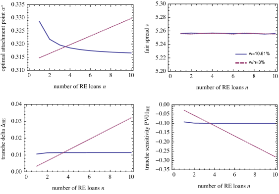
Figure 2: Tranche properties as a function of the number of loans. Solid: RE loan weight $w=10.61\%$ is fixed ( each loan has weight $w/n$); dashed: each loan has constant weight of $w/n=3\%$. Top left: optimal attachment point $\alpha^{\ast}$; top right: fair spread $s$; bottom left: tranche delta $\Delta_{RE}$; bottom right: tranche sensitivity $\text{PV01}_{RE}$.

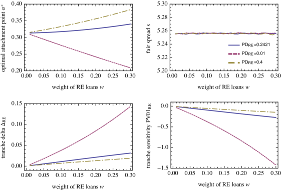
Figure 3: Tranche properties as a function of RE loan weight; number of loans is fixed at $n=5$; different PD’s for RE loans are assumed (see legend in top right graph). Top left: optimal attachment point $\alpha^{\ast}$; top right: fair spread $s$; bottom left: tranche delta $\Delta_{RE}$; bottom right: tranche sensitivity $\text{PV01}_{RE}$.

6 Conclusion and Outlook

We study public-private partnerships that have a CDO-like investment structure. Here, the public sector invests in the equity tranche, while institutional investors would typically invest in the senior tranches. The risk transfer from restructuring the asset pool’s cash flows makes the investment attractive or accessible for risk-averse institutional investors. These types of financial vehicles have been issued in a development finance context, with an explicit goal to promote financing of RE projects in emerging and developing countries. The asset pool is primarily composed of loans to regional banks, which in turn provide direct financing of RE investments. Typically, only few direct investments in RE projects are contained in the asset pool. As such, although the investment into the structured fund is channelled into RE projects, this asset pool composition creates a sensitivity mainly to banks in developing and emerging markets, and to the RE sector only to a lesser extent. Assuming that investors would also seek exposure to RE, the paper provides an answer to questions revolving around the optimal asset pool setup and structuring.

First, we develop a framework for studying this type of problem by introducing the LH++ model, a Merton-type model in which the asset pool consists of an infinitely granular homogeneous portfolio of bank exposures and one or several large direct RE investment. We derive closed formulas for CDO tranche valuation, which in turn allow to calculate sensitivities such as tranche deltas and PV01’s against RE loans. Increasing the proportion of the direct investment increases the RE exposure. However, since direct investments are larger, this also decreases diversification in the asset pool, which potentially decreases the size of the senior tranche (which is characterised by a target AAA rating).

In our stylised framework, we determine the optimal asset pool mix, which maximises RE exposure given a minimum senior tranche size and a desired rating. We show that, in a typical setting, where RE loans have a lower credit quality than bank loans, the optimal proportion of RE loans has weight smaller than $1$.

Appendix A Proof of Proposition 3

Lemma 6.

Let $X$ and $Y$ be independent, standard normally distributed random variables. Then,

$${\mathbb{E}}\left[X\,{\bf e}^{\sigma_{X}X}\right] =\sigma_{X}\,{\bf e}^{\sigma_{X}^{2}/2}$$

$${\mathbb{E}}\left[X\,{\bf e}^{\sigma_{X}X+\sigma_{Y}Y}\right] =\sigma_{X}\,{\bf e}^{\sigma_{X}^{2}/2+\sigma_{Y}^{2}/2}.$$

Proof.

The first identity is easily calculated to be

$${\mathbb{E}}\left[X\,{\bf e}^{\sigma X}\right]=\frac{1}{\sqrt{2\pi}}\int x\,{\bf e}^{\sigma_{X}x}{\bf e}^{-x^{2}/2}\,{\rm d}x=\frac{1}{\sqrt{2\pi}}\int x\,{\bf e}^{\sigma_{X}^{2}/2}\,{\bf e}^{-\frac{(x-\sigma_{X})^{2}}{2}}\,{\rm d}x=\sigma_{X}\,{\bf e}^{\sigma_{X}^{2}/2}.$$

Using this, the second identity is calculated as

$${\mathbb{E}}\left[X\,{\bf e}^{\sigma_{X}X+\sigma_{Y}Y}\right] =\frac{1}{\sqrt{2\pi}}\frac{1}{\sqrt{2\pi}}\int\int x\,{\bf e}^{\sigma_{X}X+\sigma_{Y}y}{\bf e}^{-x^{2}/2}{\bf e}^{-y^{2}/2}\,{\rm d}x\,{\rm d}y$$

$$=\frac{1}{\sqrt{2\pi}}\frac{1}{\sqrt{2\pi}}\int{\bf e}^{\sigma_{Y}y}\,{\bf e}^{-y^{2}/2}\,{\rm d}y\,\int x\,{\bf e}^{\sigma_{X}x}\,{\bf e}^{-x^{2}/2}\,{\rm d}x$$

$$={\bf e}^{\sigma_{Y}^{2}/2}\,\sigma_{X}\,{\bf e}^{\sigma_{X}^{2}/2}.$$

∎

Proof of Proposition 3.

Let $W^{B}$ and $W^{R}$ be the Brownian motions driving the respective asset processes. In the calculations below, write $W^{R}=\rho_{RB}W_{1}^{B}+\sqrt{1-\rho_{RB}^{2}}Z$, with $Z\sim{\rm N}(0,1)$ independent of $W_{1}^{B}$. Recall that the variance of a log-normally distributed random variable ${\bf e}^{X}$ with $X\sim{\rm N}(0,\sigma^{2})$ is ${\bf e}^{\sigma^{2}}({\bf e}^{\sigma^{2}}-1)$. The variance of the right-hand side of (20) is given by

$$\text{Var}\left(\ln(A_{1})+\frac{R_{1}}{A_{1}}\right)=\text{Var}\left((r-\frac{1}{2}\sigma_{B}^{2})+\sigma_{B}W_{1}^{B}+\frac{R_{0}}{A_{0}}{\bf e}^{(r-1/2\sigma_{R}^{2})+\sigma_{R}W_{1}^{R}-(r-1/2\sigma_{B}^{2})-\sigma_{B}W_{1}^{B}}\right)\\ \begin{aligned} &=\sigma_{B}^{2}+\frac{R_{0}^{2}}{A_{0}^{2}}{\bf e}^{(\sigma_{B}^{2}-\sigma_{R}^{2})}\,\text{Var}\left({\bf e}^{(\rho_{RB}\sigma_{R}-\sigma_{B})W_{1}^{B}+\sqrt{1-\rho_{RB}^{2}}\sigma_{R}Z}\right)\\ &\phantom{=\,}+2\,\sigma_{B}\,\frac{R_{0}}{A_{0}}\,{\bf e}^{(\sigma_{B}^{2}-\sigma_{R}^{2})/2}\,\text{Cov}\left(W_{1}^{B},{\bf e}^{(\rho_{RB}\sigma_{R}-\sigma_{B})W_{1}^{B}+\sqrt{1-\rho_{RB}^{2}}\sigma_{R}Z}\right)\\ &=\sigma_{B}^{2}+\frac{R_{0}^{2}}{A_{0}^{2}}{\bf e}^{(\sigma_{B}^{2}-\sigma_{R}^{2})}{\bf e}^{(\rho_{RB}\sigma_{R}-\sigma_{B})^{2}+(1-\rho_{RB}^{2})\sigma_{R}^{2}}({\bf e}^{(\rho_{RB}\sigma_{R}-\sigma_{B})^{2}+(1-\rho_{RB}^{2})\sigma_{R}^{2}}-1)\\ &\phantom{=\,}+2\sigma_{B}\frac{R_{0}}{A_{0}}{\bf e}^{(\sigma_{B}^{2}-\sigma_{R}^{2})/2}(\rho_{RB}\sigma_{R}-\sigma_{B}){\bf e}^{((\rho_{RB}\sigma_{R}-\sigma_{B})^{2}+\sigma_{R}^{2}(1-\rho_{RB}^{2}))/2}\\ &=\sigma_{B}^{2}+\frac{R_{0}^{2}}{A_{0}^{2}}{\bf e}^{2\sigma_{B}(\sigma_{B}-\rho_{RB}\sigma_{R})}({\bf e}^{\sigma_{B}^{2}+\sigma_{R}^{2}-2\rho_{RB}\sigma_{B}\sigma_{R}}-1)+2\sigma_{B}\frac{R_{0}}{A_{0}}(\rho_{RB}\sigma_{R}-\sigma_{B}){\bf e}^{\sigma_{B}^{2}-\rho_{RB}\sigma_{R}\sigma_{B}}.\end{aligned}$$

For the correlation we calculate the required covariance. In the calculations we decompose the (correlated) vector $\mathbf{W}^{T}=(W_{1}^{B,i},W_{1}^{B,j},W_{1}^{R,i},W_{1}^{R,j})^{T}$ into a Cholesky factorisation $\mathbf{C}$ with independent normals $\mathbf{Z}^{T}=(Z_{1},\ldots,Z_{4})^{T}$:

$$\mathbf{W}=\mathbf{C}\cdot\mathbf{Z},$$

where

$$C=\begin{pmatrix}1&0&0&\\ \rho_{B}&\sqrt{1-\rho_{B}^{2}}&0&0\\ \rho_{RB}&\rho_{RB}\frac{1-\rho_{B}}{\sqrt{1-\rho_{B}^{2}}}&\sqrt{\frac{1+\rho_{B}-2\rho_{RB}^{2}}{1+\rho_{B}}}&0\\ \rho_{RB}&\rho_{RB}\frac{1-\rho_{B}}{\sqrt{1-\rho_{B}^{2}}}&\frac{\rho_{R}+\rho_{R}\rho_{B}-2\rho_{RB}^{2}}{\sqrt{(1+\rho_{B})(1+\rho_{B}-2\rho_{RB}^{2})}}&\sqrt{\frac{(1+\rho_{B})(1-\rho_{R}^{2})-4\rho_{RB}^{2}(1+\rho_{R})}{1+\rho_{B}-2\rho_{RB}^{2}}}\end{pmatrix}.$$

The covariance is given by:

$$\text{Cov}\left(\ln(A_{1}^{i})+\frac{R_{1}^{i}}{A_{1}^{i}},\ln(A_{1}^{j})+\frac{R_{1}^{j}}{A_{1}^{j}}\right)\\ \begin{aligned} &=\text{Cov}\left(\sigma_{B}W_{1}^{B,i},\sigma_{B}W_{1}^{B,j}\right)+2\text{Cov}\left(\sigma_{B}W_{1}^{B,i},\frac{R_{0}}{A_{0}}{\bf e}^{(\sigma_{B}^{2}-\sigma_{R}^{2})/2+\sigma_{R}W_{1}^{j,R}-\sigma_{B}W_{1}^{j,B}}\right)\\ &\phantom{=\,}+\text{Cov}\left(\frac{R_{0}}{A_{0}}{\bf e}^{(\sigma_{B}^{2}-\sigma_{R}^{2})/2+\sigma_{R}W_{1}^{i,R}-\sigma_{B}W_{1}^{i,B}},\frac{R_{0}}{A_{0}}{\bf e}^{(\sigma_{B}^{2}-\sigma_{R}^{2})/2+\sigma_{R}W_{1}^{j,R}-\sigma_{B}W_{1}^{j,B}}\right)\\ &=\rho_{B}\sigma_{B}^{2}+2\sigma_{B}\frac{R_{0}}{A_{0}}{\bf e}^{(\sigma_{B}^{2}-\sigma_{R}^{2})/2}\text{Cov}\left(Z_{1},{\bf e}^{\sigma_{R}(c_{41}Z_{1}+c_{42}Z_{2}+c_{43}Z_{3}+c_{44}Z_{4})-\sigma_{B}(c_{21}Z_{1}+c_{22}Z_{2})}\right)\\ &\phantom{=\,}+\frac{R_{0}^{2}}{A_{0}^{2}}{\bf e}^{(\sigma_{B}^{2}-\sigma_{R}^{2})}\text{Cov}\left({\bf e}^{\sigma_{R}(c_{31}Z_{1}+c_{32}Z_{2}+c_{33}Z_{3})-\sigma_{B}Z_{1}},{\bf e}^{\sigma_{R}(c_{41}Z_{1}+c_{42}Z_{2}+c_{43}Z_{3}+c_{44}Z_{4})-\sigma_{B}(c_{21}Z_{1}+c_{22}Z_{2})}\right)\\ &=\rho_{B}\sigma_{B}^{2}+2\sigma_{B}\frac{R_{0}}{A_{0}}{\bf e}^{(\sigma_{B}^{2}-\sigma_{R}^{2})/2}(\sigma_{R}c_{41}-\sigma_{B}c_{21}){\bf e}^{((\sigma_{R}c_{41}-\sigma_{B}c_{21})^{2}+(\sigma_{R}c_{42}-\sigma_{B}c_{22})^{2}+\sigma_{R}^{2}c_{43}^{2}+\sigma_{R}^{2}c_{44}^{2})/2}\\ &\phantom{=\,}+\frac{R_{0}^{2}}{A_{0}^{2}}{\bf e}^{(\sigma_{B}^{2}-\sigma_{R}^{2})}{\bf e}^{((\sigma_{R}c_{31}-\sigma_{B}+\sigma_{R}c_{41}-\sigma_{B}c_{21})^{2}+(\sigma_{R}c_{32}+\sigma_{R}c_{42}-\sigma_{B}c_{22})^{2}+(\sigma_{R}c_{33}+\sigma_{R}c_{43})^{2}+\sigma_{R}^{2}c_{44}^{2})/2}\\ &\phantom{=\,}-\frac{R_{0}^{2}}{A_{0}^{2}}{\bf e}^{(\sigma_{B}^{2}-\sigma_{R}^{2})}{\bf e}^{((\sigma_{R}c_{31}-\sigma_{B})^{2}+\sigma_{R}^{2}c_{32}^{2}+\sigma_{R}^{2}c_{33}^{2}+(\sigma_{R}c_{41}-\sigma_{B}c_{21})^{2}+(\sigma_{R}c_{42}-\sigma_{B}c_{22})^{2}+\sigma_{R}^{2}c_{43}^{2}+\sigma_{R}^{2}c_{44}^{2})/2}\\ &=\rho_{B}\sigma_{B}^{2}+2\sigma_{B}\frac{R_{0}}{A_{0}}{\bf e}^{\sigma_{B}^{2}-\rho_{RB}\sigma_{B}\sigma_{R}}(\rho_{RB}\sigma_{R}-\rho_{B}\sigma_{B})+\frac{R_{0}^{2}}{A_{0}^{2}}{\bf e}^{2\sigma_{B}^{2}-2\rho_{RB}\sigma_{B}\sigma_{R}}\left({\bf e}^{\rho_{B}\sigma_{B}^{2}+\rho_{R}\sigma_{R}^{2}-2\rho_{RB}\sigma_{B}\sigma_{R}}-1\right).\end{aligned}$$

The correlation is obtained by dividing by the respective variance.

For the correlation of the modified bank’s balance sheet with a single RE loan, we obtain

$$\text{Cov}\left(\ln(A_{1}^{i})+\frac{R_{1}^{i}}{A_{1}^{i}},\ln(R_{1})\right)\\ \begin{aligned} &=\text{Cov}\left(\sigma_{B}W_{1}^{i,B}+\frac{R_{0}}{A_{0}}{\bf e}^{(\sigma_{B}^{2}-\sigma_{R}^{2})/2+\sigma_{R}W_{1}^{i,R}-\sigma_{B}W_{1}^{i,B}},\sigma_{R}W_{1}^{j,R}\right)\\ &=\rho_{RB}\sigma_{B}\sigma_{R}+\frac{R_{0}}{A_{0}}{\bf e}^{(\sigma_{B}^{2}-\sigma_{R}^{2})/2}\sigma_{R}\text{Cov}\left({\bf e}^{\sigma_{R}W_{1}^{i,R}-\sigma_{B}W_{1}^{i,B}},W_{1}^{j,R}\right)\\ &=\rho_{RB}\sigma_{B}\sigma_{R}+\sigma_{R}\frac{R_{0}}{A_{0}}{\bf e}^{(\sigma_{B}^{2}-\sigma_{R}^{2})/2}\text{Cov}\left({\bf e}^{(\sigma_{R}c_{31}-\sigma_{B})Z_{1}+\sigma_{R}c_{32}Z_{2}+\sigma_{R}c_{33}Z_{3}},c_{41}Z_{1}+c_{42}Z_{2}+c_{43}Z_{3}+c_{44}Z_{4}\right)\\ &=\rho_{RB}\sigma_{B}\sigma_{R}+\sigma_{R}\frac{R_{0}}{A_{0}}{\bf e}^{(\sigma_{B}^{2}-\sigma_{R}^{2})/2}\Big{\{}(\sigma_{R}c_{31}-\sigma_{B})c_{41}{\bf e}^{((\sigma_{R}c_{31}-\sigma_{B})^{2}+\sigma_{R}^{2}c_{32}^{2}+\sigma_{R}^{2}c_{33}^{2})/2}\Big{.}\\ &\phantom{=\,}\Big{.}+\sigma_{R}c_{32}c_{42}{\bf e}^{(\sigma_{R}^{2}c_{32}^{2}+(\sigma_{R}c_{31}-\sigma_{B})^{2}+\sigma_{R}^{2}c_{33}^{2})/2}+\sigma_{R}c_{33}c_{43}{\bf e}^{(\sigma_{R}^{2}c_{33}^{2}+(\sigma_{R}c_{31}-\sigma_{B})^{2}+\sigma_{R}^{2}c_{32}^{2})/2}\Big{\}}\\ &=\rho_{RB}\sigma_{B}\sigma_{R}+\sigma_{R}\frac{R_{0}}{A_{0}}{\bf e}^{(\sigma_{B}^{2}-\sigma_{R}^{2})/2}\left((\sigma_{R}c_{31}-\sigma_{B})c_{41}+\sigma_{R}c_{32}c_{42}+\sigma_{R}c_{33}c_{43}\right){\bf e}^{((\sigma_{R}c_{31}-\sigma_{B})^{2}+\sigma_{R}^{2}c_{32}^{2}+\sigma_{R}^{2}c_{33}^{2})/2}\\ &=\rho_{RB}\sigma_{B}\sigma_{R}+\sigma_{R}\frac{R_{0}}{A_{0}}{\bf e}^{\sigma_{B}^{2}-\rho_{RB}\sigma_{B}\sigma_{R}}(\rho_{R}\sigma_{R}-\rho_{RB}\sigma_{B}).\end{aligned}$$

The correlation is obtained by dividing by the respective standard deviations. ∎

References

• Andersen and Sidenius (2004) L. Andersen and J. Sidenius. Extensions to the gaussian copula: Random recovery and random factor loadings. Journal of Credit Risk, 1(1):29–70, 2004.
• Bluhm et al. (2003) C. Bluhm, L. Overbeck, and C. Wagner. An Introduction to Credit Risk Modeling. Chapman & Hall/CRC, London, 2003.
• Bluhm (2003) C. Bluhm. CDO modeling: Techniques, examples and applications. Working Paper, December 2003.
• Dorfleitner et al. (2011) G. Dorfleitner, M. Leidl, and C. Priberny. Microcredit as an asset class: structured microfinance. In Mobilising Capital for Emerging Markets, pages 137–154. Springer, 2011.
• Duffie and Singleton (2003) D. Duffie and K. J. Singleton. Credit Risk: Pricing, Measurement, and Management. Princeton University Press, 2003.
• Düllmann et al. (2008) K. Düllmann, M. Scheicher, and C. Schmieder. Asset correlations and credit portfolio risk: an empirical analysis. Journal of Credit Risk, 4(2):37–63, 2008.
• Global Climate Partnership Fund (2019) Global Climate Partnership Fund. Quarterly Report Q3 2019. Report, 2019.
• Gordy (2003) M. B. Gordy. A risk-factor model foundation for ratings-based bank capital rules. Journal of Financial Intermediation, 12(3):199–232, 2003.
• Greenberg et al. (2004) A. Greenberg, D. O’Kane, and L. Schloegl. LH+: a fast analytical model for CDO hedging and risk management. Lehman Brothers Quantitative Credit Research Quarterly, Q2:19–31, 2004.
• Gregory and Laurent (2004) J. Gregory and J.-P. Laurent. In the core of correlation. RISK, 17(10):87–91, 2004.
• Hull and White (2007) J. Hull and A. White. Dynamic models of portfolio credit risk: A simplified approach. Working Paper, May 2007.
• Hull and White (2010) J. Hull and A. White. The risk of tranches created from mortgages. Financial Analysts Journal, 66(5):54–67, 2010.
• Krauss and Walter (2009) N. Krauss and I. Walter. Can microfinance reduce portfolio volatility? Economic Development and Cultural Change, 58(1):85–110, 2009.
• Li (2000) D. X. Li. On Default Correlation: A Copula Function Approach. The Journal of Fixed Income, pages 43–54, March 2000.
• Merton (1974) R. C. Merton. On the pricing of corporate debt: The risk structure of interest rates. The Journal of Finance, 29(2):449–470, May 1974.
• O’Kane (2008) D. O’Kane. Modelling Single-name and Multi-name Credit Derivatives. Wiley, 2008.
• S&P Global Ratings (2015) S&P Global Ratings. Global methodologies and assumptions for corporate cash flow and synthetic CDOs. Report, September 2015.
• S&P Global Ratings (2019) S&P Global Ratings. 2018 annual global corporate default and rating transition study. Report, April 2019.
• Vasicek (1987) O. Vasicek. Probability of loss on loan portfolio. KMV Corporation, 1987.
• Vasicek (1991) O. Vasicek. Limiting loan loss probability distribution. KMV Corporation, 1991.