Floor- or ceiling-sliding for chemically active, gyrotactic, sedimenting Janus particles

Abstract

Chemically active particles achieve motility without external forces and torques (“self-propulsion”) due to catalytic chemical reactions at their surfaces, which change the chemical composition of the surrounding solution (called “chemical field“) and induce hydrodynamic flow of the solution. By coupling the distortions of these fields back to its motion, a chemically active particle experiences an effective interaction with confining surfaces. This coupling can lead to a rich behavior, such as the occurrence of wall-bound steady states of “sliding”.

Most active particles are density mismatched with the solution, and thus tend to sediment. Moreover, the often employed Janus spheres, which consist of an inert core material decorated with a cap-like, thin layer of a catalyst, are gyrotactic (i.e., “bottom-heavy”). Whether or not they may exhibit sliding states at horizontal walls depends on the interplay between the active motion and the gravity-driven sedimentation and alignment, such as the gyrotactic tendency to align the axis along the gravity direction being overcome by a competing, activity-driven alignment with a different orientation. It is therefore important to understand and quantify the influence of these gravity-induced effects on the behavior of model chemically active particles moving in the vicinity of walls.

For model gyrotactic, self-phoretic Janus particles, here we study theoretically the occurrence of sliding states at horizontal planar walls that are either below (“floor”) or above (“ceiling”) the particle. We construct “state diagrams” characterizing the occurrence of such states as a function of the sedimentation velocity and of the gyrotactic response of the particle, as well as of the phoretic mobility of the particle. We show that in certain cases sliding states may emerge simultaneously at both the ceiling and the floor, while the larger part of the experimentally relevant parameter space corresponds to particles that would exhibit sliding states only either at the floor or at the ceiling – or there are no sliding states at all. These predictions are critically compared with the results of previous experimental studies, as well as with our dedicated experiments carried out with Pt-coated, polystyrene-core or silica-core Janus spheres immersed in aqueous hydrogen peroxide solutions.

^∗ Corresponding authors

IV. Institut für Theoretische Physik, Universität Stuttgart, Pfaffenwaldring 57, D-70569 Stuttgart, Germany

1 Introduction

Since the first reports of self-motility for micrometer-sized colloids appeared fifteen years ago ^{1, 2}, the topics of active particles, active fluids, and active matter have witnessed a rapid growth of scientific interest. A wide variety of such particles, which are capable of moving autonomously, i.e., in the absence of external forces or torques acting on them or on the fluid, within a liquid environment – by promoting chemical reactions involving their surrounding solution – has been proposed and studied experimentally; see the thorough and insightful reviews provided in Refs. 3, 4, 5, 6. One of the often encountered experimental realizations is that of spherical, axisymmetric Janus colloids, which self-propel when immersed in an aqueous hydrogen peroxide ($\mathrm{H_{2}O_{2}}$) solution. These particles are obtained by depositing a thin film of catalyst material over a spherical core of a material without catalytic properties. The deposition of the main, catalytic material is sometimes preceded by that of an ultrathin layer of a material, which facilitates the adhesion of the catalyst, such as Ti on polystyrene before depositing Pt (see, e.g., Ref. 9). Typical realizations, which will be of main interest for the present study, are Pt on polystyrene (Pt/PS) particles ^{8, 9, 10, 11, 12, 13} and Pt on silica (Pt/$\mathrm{SiO_{2}}$) particles ^{14, 15, 16, 17, 18}; another example, which is recently attracting much interest, is that of titania on silica ($\mathrm{TiO_{2}}$/$\mathrm{SiO_{2}}$) particles ^{19, 20}, for which the decomposition of $\mathrm{H_{2}O_{2}}$ occurs via photocatalysis upon illumination with UV light of a suitable wavelength. The reviews in Refs. 5, 6, and 21 provide detailed accounts and exhaustive lists of references of the numerous other types (with respect to core and catalyst) of Janus particles reported in experimental studies, as well as of the various mechanisms of self-motility.

Irrespective of the exact mechanism of motion, the motility of chemically active Janus particles is connected with hydrodynamic flow of the solution as well as with a spatially varying distribution of chemical species (“chemical field”) around the particle. When such particles operate in the vicinity of walls, or, in general, near any type of spatially confining boundary, their chemical and hydrodynamic fields are distorted due to the impenetrability of the wall and due to the no-slip hydrodynamic condition at the wall. The coupling of these disturbances back to the particle influences its motion, i.e., the particle experiences an effective interaction with the confining boundary (see, e.g., the review in Ref. 22). For axially symmetric Janus colloids, one of the most striking consequences of these interactions is the occurrence of steady-states of sliding along the wall, in which the particle moves parallel to the wall while maintaining a constant distance from it and a constant orientation of its axis relative to the direction normal to the wall. Such states, predicted theoretically in Ref. 23 for particles moving by self-phoresis, have been observed in experiments with Janus particles ^{24, 9, 15, 11, 12, 25, 26, 19, 20, 27} and provide the rationale behind concepts such as “guidance” by topographical features ^{15, 28, 18, 27} or rheotactic behavior of spherical Janus colloids ^{29, 30}. (Note that the experiments in Refs. 12 and 27, and a part of those in Ref. 26, involve setups with chemically active Janus particles in the vicinity of a fluid interface; in such cases, additional contributions to the sliding state, emerging from, e.g., induced Marangoni flows ³¹, are expected to play a role.)

A common characteristic of the spherical Janus colloids discussed above is that they are “bottom heavy”, owing to the mismatch in density between the catalyst layer and the core material. This bottom heaviness leads to a gyrotactic response, i.e., a torque that rotates the axis of the particle towards alignment with the direction of gravity; accordingly, such a Janus particle immersed in solution exhibits a preferred orientation with the cap of catalyst (typically the denser material) pointing into the direction of gravity ¹⁰. (Note that this effect occurs in addition to the emergence of polar alignment along the gravity direction, as reported in Refs. 32 and 33, which is due to the interplay between sedimentation, self-motility, and thermal fluctuations. Furthermore, an interplay between self-propulsion, sedimentation, and shape lacking axial symmetry can also lead to very complex patterns of gravitaxis or cross-gravitaxis, i.e., motion orthogonal to the direction of gravity, as reported by studies with L-shaped particles ³⁴.) Such particles have the potential to mimic the behavior of “bottom heavy” motile micro-organisms, such as Chlamydomonas, which are known to exhibit very interesting collective dynamics via the interplay of self-motility with the gyrotactic and gravitactic response to gravity as an external aligning field. Theoretical studies of heavy and bottom-heavy hydrodynamic squirmers have been successful in capturing phenomena exhibited by swimming microorganisms, such as the “dancing” of Volvox algae ³⁵. Collective alignment and self-assembly into spinners have been reported for monolayers of heavy squirmers ³⁶, and the stability of such monolayers has been thoroughly analyzed ³⁷. Finally, we note that recently the collective sedimentation of squirmers under gravity ³⁸ and the sedimentation of a heavy squirmer in the vicinity of a wall ³⁹ have been studied.

Returning to the case of chemically active particles and their dynamics in the vicinity of a wall, we note that in the absence of gravity-induced effects the chemical and hydrodynamic interactions of the active Janus particle with the wall lead to an orientation of the axis of the Janus particle, which is typically within $\pm 30^{\circ}$ from being parallel to the wall ^{23, 40, 41}. In the presence of gravity, a bottom heavy Janus particle experiences in addition the competing effect of the gyrotactic preference for alignment of its axis along the direction of gravity, which is perpendicular to a horizontal wall; see Fig. 1. (Obviously, any particle, which is not density matched with the liquid, experiences also a gravitational force.) Accordingly, this raises the question of whether, for model chemically active Janus particles and upon accounting for the effects due to gravity, sliding states along a horizontal wall still occur.

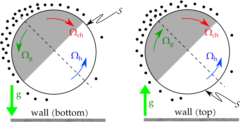
Figure 1: Schematic illustration of a spherical, chemically active, gyrotactic (bottom heavy) Janus particle approaching (left panel) a bottom wall (“floor”) or (right panel) a top wall (“ceiling”). As depicted in the right panel, the configuration of approaching a “ceiling” is similar to that of approaching a “floor”, except for a reversal of the direction of gravity (and thus of the gyrotactic response, i.e., the green arrows). The use of this equivalence is advantageous because the definition of the configuration of the particle (i.e., the height above the wall and the orientation with respect to the wall) involves in both cases the same variables $h$ and $\theta$ (see the main text). The chemical activity is modeled as the release, at the catalyst side (dark gray area) of the surface $\mathcal{S}$ of the particle, of solute molecules (black dots) into the surrounding solution. (As depicted in the figure, the distributions of solute at a given configuration ($h$, $\theta$) are the same for a particle below the ceiling or above the wall.) The rotations due to hydrodynamic (blue arrow) and chemical (red arrow) effective interactions with the wall (i.e, the coupling of the wall-induced distortions of the chemical and the flow fields to the motion of the particle), respectively, are shown for the case in which they oppose each other, and thus could eventually balance in the absence of gravity (as in the case, e.g., of a sliding state along a vertical wall).

For particles that sediment to the floor, there is ample experimental evidence for sliding states ^{15, 19, 18, 9}. Theoretical studies, which employ simple models of self-phoretic, gyrotactic Janus particles, capture this phenomenology ^{15, 19}. For example, it has been shown that, for parameters corresponding to a typical Pt/$\mathrm{SiO_{2}}$ particle, (i) the model self-phoretic particle employed in Ref. 23 – augmented with terms accounting for sedimentation and bottom heaviness – predicts the emergence of sliding states; and (ii) for the sliding state, the rotation of the axis due to the gravitational torque, and the rotations due to the chemical and hydrodynamic interactions of the particle with the wall, are all comparable in magnitude.

The correlation of the latter observation with the changes of sign within the effects of gravity at the ceiling and at the floor (e.g., compare the gyrotactic response, indicated by green arrows, in the panels of Fig. 1), leads to an important conclusion: the question concerning the emergence of sliding states cannot be answered based solely on the behavior at the floor, even if the latter is completely understood. Accordingly, an additional study is required in order to understand if the models employed in the theoretical analysis are also compatible with the experimental observations of sliding states occurring at upper planar boundaries (ceiling)^{11, 12, 28, 25}.

Additional motivation for such a study arises from the question of how active particles, which are both heavy (i.e., they sediment to the floor in the absence of chemical “fuel”) and bottom-heavy (i.e., there is a gravitational torque due to the catalytic cap), may reach a state of sliding at the ceiling. One scenario, applicable for active particles moving with the active cap at the back, is the following. At sufficiently strong chemical activity, and thus at high velocity of self-propulsion, the particles lift off from the floor and, owing to the bottom-heavy gyrotactic response aligning their caps down, exhibit a persistent three-dimensional motion against gravity (see, e.g., the experimental reports in Refs. 11, 10, 19, 25). This leads to collisions with the ceiling, which is a prerequisite for the emergence of a sliding state^{23, 15, 42}; obviously, in this regime of chemical activity the sliding states at the floor cease to exist. The issue is whether the above lift-off scenario is actually a necessary condition for the occurrence of a sliding state at the ceiling. For example, one can think of an alternative scenario in which active particles sediment in the bulk, i.e., far from confining boundaries gravity dominates self-propulsion, but a state of sliding at the ceiling exists. In this scenario, an active particle, which is initially located within the basin of attraction of that state, will end up sliding along the ceiling, even though the chemical activity is not strong enough to ensure a lift-off from the floor. This scenario, that for given material properties – e.g., Pt/PS particles of a given radius and a given chemical activity, i.e., a fixed concentration of H₂O₂ – sliding states at the floor coexist with sliding states at the ceiling, so far has not been explored theoretically. Yet, it would rationalize the observation, in the context of a single experiment, of motile Janus particles both at the top and at the bottom walls. Such a situation can be inferred from the studies in Refs. 11 and 28.

The discussion above illustrates a complex interplay between the chemical activity of the Janus particle, the effects due to gravity (sedimentation and gyrotactic alignment), and the vertical location of the bounding wall with respect to the particle, i.e., whether it is above or below the particle. This can affect both qualitatively and quantitatively the emergent dynamical behavior. It is therefore important to understand and quantify the influence of these gravity-induced effects on the behavior of model chemically active particles moving in the vicinity of walls. Here, we study both theoretically and experimentally, for model bottom heavy, self-phoretic Janus particles, the issue of the occurrence of sliding states at planar, horizontal floor and ceiling walls. We use a simple model of self-phoretic motion ⁴³, which has been previously shown to capture qualitatively the behavior exhibited in experimental studies of Janus particles near walls ^{15, 18, 19}. For two choices of the chemical activity of the particle, which are typically invoked in theoretical studies ^{43, 44, 45, 46}, we construct “state diagrams”. They summarize the behavior of the model gyrotactic, self-phoretic Janus particles near walls as functions of the relevant parameters of the dynamics. These parameters are the ratios between activity- and gravity-induced translational and rotational velocities, and the ratio of the phoretic mobilities of the active and inert parts of the Janus particle. The theoretical predictions are critically compared with the results of the present experiments conducted with Pt/PS and Pt/SiO₂ Janus particles immersed in aqueous H₂O₂ solutions, as well as with previously published experimental studies in which sliding states at the ceiling have been reported ^{11, 28, 25}.

2 Experimental section

Polystyrene latex particles of two sizes, radii $R=1.2~{}\mathrm{\mu m}$ and $2.5~{}\mathrm{\mu m}$, respectively, as well as silica particles of $R=0.5~{}\mathrm{\mu m}$ and $2~{}\mathrm{\mu m}$, respectively, are employed in the study. Janus particles are fabricated by using the physical vapor deposition (PVD) technique to coat the spherical polystyrene (or silica) particles with platinum. In brief, for each type and size of particle, a monolayer of them is assembled onto a pre-cleaned glass slide using the convective assembly method ⁴⁷. Subsequently, these monolayers of particles are exposed to platinum vapor in a PVD machine (Ted Pella), and a quantity of Pt – equivalent to a planar layer of thickness $\delta_{rep}\simeq 9~{}\mathrm{nm}$ (as reported by the device) – is deposited onto such a monolayer of particles. After the Pt deposition, the Janus particles formed this way are dispersed in deionized water by sonicating the glass slides for one minute.

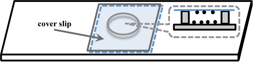
Figure 2: Sketch of the experimental cell (height of $\approx 500~{}\mathrm{\mu m}$, volume of $\approx 40~{}\mathrm{\mu l}$). The inset illustrates the vertical cross section of the cell, with the black dots depicting active particles at the top (blue) and bottom (gray) glass slides.

The experimental cell used to study the motion of the particles, while they are suspended in an aqueous $\mathrm{H_{2}O_{2}}$ solution, is composed of a glass slide and a silicone isolator ring (Invitrogen Corp.). The silicone ring is attached onto a pre-cleaned glass slide with the help of an adhesive added onto its bottom surface, creating a cylindrical well of approximately 9 mm diameter and 0.5 mm depth (see Fig. 2). The large height of the cell (at least 100 particle diameters, for the particles employed in our study) ensures that the dynamics of an active particle in the vicinity of one of the walls (top or bottom) is, to a very good approximation, unaffected by the presence of the other, distant wall.

The concentration of the aqueous dispersion of Janus particles is adjusted to $\lesssim 1\%$ volume fraction; the use of a very dilute particle suspension ensures that the experiments are exploring the regime of “single particle motion”, and it also reduces the probability of forming bubbles (which would give rise to spurious motions of nearby particles). Subsequently, the particle suspension is mixed with an adequate volume of aqueous hydrogen peroxide solution, in order to obtain the desired $\mathrm{H_{2}O_{2}}$ concentration, as follows. First, an aqueous solution of 6% (v/v) concentration $\mathrm{H_{2}O_{2}}$ is prepared from an aqueous stock solution of 30% $\mathrm{H_{2}O_{2}}$ (Fisher Scientific). A volume of the dispersion of Janus particles is then gently mixed with an equal volume of the aqueous 6% (v/v) $\mathrm{H_{2}O_{2}}$ solution, resulting in a 3% (v/v) $\mathrm{H_{2}O_{2}}$ suspension of Janus particles. Subsequently, the well-mixed solution is transferred to the well by means of a pipette, and the well is carefully covered with a cover slip in order to avoid disturbances due to air currents and to reduce water evaporation. Moreover, the top cover slip provides the “ceiling” wall for studying the eventual emergence of sliding states at the top.

Since the self-propelled motion of the particles starts immediately upon mixing of the particle suspension with the aqueous $\mathrm{H_{2}O_{2}}$ solution, the particles are already motile when the mixed solution is placed into the experimental well. Consequently, this setup provides optimal conditions for the eventual occurrence of sliding states at the upper cover slip, because the distribution of motile particles within the volume is relatively uniform at the beginning of the experiment.

The motion of the Janus particles is observed using an Olympus BX-51 microscope with a $\times 20$ objective and it is recorded with an u-eye 2240c camera at a rate of 10 frames per second (fps). In order to capture only the motion near the bottom wall or the top wall, respectively, the focal plane of the microscope is adjusted correspondingly and only the motion of those particles that remain in focus is used to determine the self-propulsion velocity. The latter is obtained by following Ref. 8: from the tracked two-dimensional trajectories of the particles along the wall, as shown in, c.f., Figs. 11 and 12, the mean square displacement as a function of time is determined. The velocity $U$ is obtained by fitting the time dependence with the active Brownian motion model introduced in Ref. 8. In these calculations, we have employed between 40 to 60 tracked trajectories, for each particle type, size, and location (at the floor or, if occurring, at the ceiling) of the sliding state. For Pt/PS particles, we obtain $U_{PS}\approx 1.5\pm 0.4~{}\mathrm{\mu m/s}$, for particles of both sizes and for sliding states at both the floor and the ceiling walls (see, c.f., the section on results and discussion); for Pt/SiO₂ particles sliding at the floor (no sliding along the ceiling has been observed), the values obtained depend on the size of the particle: $U_{Si}\approx 2.1\pm 0.6~{}\mathrm{\mu m/s}$ for the small ($R=0.5~{}\mathrm{\mu m}$) particles, and $\approx 1.4\pm 0.4~{}\mathrm{\mu m/s}$ for the large ($R=2~{}\mathrm{\mu m}$) ones. These velocities compare well with simple estimates of the average velocity along the quasi-straight parts of the trajectories (see also the videos SI.V1 - SI.V7 in the Supporting Information (SI)).

3 Model and theory

As noted in the Introduction, an important question addressed in the present study is whether the phenomenology of the emergence of sliding states at the ceiling for chemically active, gyrotactic particles can be captured by the same simple models, which have been employed in the previous investigations of the behavior at the floor ^{23, 40, 16, 19, 46}. Accordingly, here we use the framework of self-phoresis and, concerning the model chemical activity, we study both the “constant flux” model, employed in previous studies ^{43, 23, 40}, as well as a model with spatially “variable flux” across the active cap. The latter model allows for a possible dependence of the catalytic activity on the local thickness of the catalytic layer. This layer is assumed to vary from being thick at the pole to being (vanishingly) thin at the equator, as proposed in Refs. 10 and 25 (for more details see below and, c.f., Fig. 4).

In brief, the chemical activity of the Janus colloid is modeled as the release, at the catalytic cap, of a molecular species into the surrounding solution. (Here it is $\mathrm{O_{2}}$ resulting from the Pt-catalyzed decomposition of $\mathrm{H_{2}O_{2}}$; the other product of the reaction is the solvent $\mathrm{H_{2}O}$.) The reaction is assumed to be within the regime of reaction-limited kinetics, and $\mathrm{H_{2}O_{2}}$ is taken to be present in abundance. This case is likely to apply for typical experiments, with very dilute particle suspensions, large volumes of solution with few percent v/v concentration of $\mathrm{H_{2}O_{2}}$, and typical duration of experiments of the order of less then 30 min.

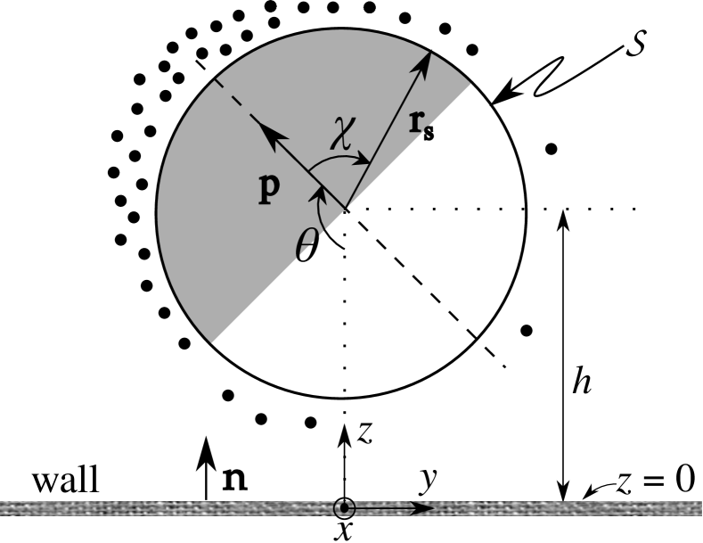
Figure 3: A spherical, chemically active Janus particle of radius $R$, with its center at (dimensionless) height $h={\tilde{h}}/R$ above a planar wall located at $z=0$ and with orientation $\theta$ defined by $\cos\theta=-\mathbf{p}\cdot\mathbf{e}_{z}$; the pair $(h,\theta)$ is referred to as “configuration”. The active (inert) part is indicated by dark gray (white) color. The location $\mathbf{r}_{s}$ on the surface $\mathcal{S}$ of the particle is parameterized by the angle $\chi$ between $\mathbf{r}_{s}$ and $\mathbf{p}$. The inner normal of the wall is shown by the unit vector $\mathbf{n}$. All lengths without tilde are measured in units of $R$, and thus they are dimensionless.

The solute molecules diffuse in the surrounding solution with diffusion coefficient $D$; the diffusion of the solute is assumed to be a very fast process compared to both the motion of the particle and the advection of the solute by the flow of the solution; i.e., for the solute transport Péclet number one has $\mathrm{Pe}:=U_{0}R/D\ll 1$, where $R$ is the radius of the particle, and $U_{0}$ is a characteristic particle velocity. Under these latter assumptions, the solute number density field relaxes quickly to a quasi-steady distribution $c(\mathbf{r})$. Assuming that $c(\mathbf{r})$ is sufficiently small, such that the chemical potential of the solute can be approximated by that of an ideal gas, the distribution $c(\mathbf{r})$ is the solution of the Laplace equation,

$$\nabla^{2}c(\mathbf{r})=0\,,~{}\mathbf{r}\in~{}\mathrm{fluid}\,,$$ (1)

subject to boundary conditions at the surface $\mathcal{S}$ of the particle, at the planar wall located at $z=0$, see Fig. 3, and at infinity (far from the particle, i.e., in the “bulk” solution). These are given by

$$[\mathbf{n}\cdot(-D\nabla c)]|_{\mathbf{r}_{s}}=\mathcal{Q}q(\mathbf{r}_{s})\,,~{}\mathbf{r}_{s}\in~{}\mathcal{S}\,,$$ (2a)

$$[\mathbf{n}\cdot(-D\nabla c)]|_{z=0}=0\,,$$ (2b)

and

$$c(|\mathbf{r}|\to\infty)=0\,,~{}\mathbf{r}\in~{}\mathrm{fluid}\,.$$ (2c)

Here, the unit vector $\mathbf{n}$ denotes the inner (i.e., oriented into the fluid) normal of the corresponding boundary (the particle surface or the wall). The dimensionless function $q(\mathbf{r}_{s})$ accounts for the geometrical distribution of the chemical activity across the surface. Accordingly, one has $q(\mathbf{r}_{s})=0$ at the locations $\mathbf{r}_{s}$ (position vector from the center of the particle, see Fig. 3) within the inert part of the surface. In addition, $q(\mathbf{r}_{s})$ takes into account possible variations of the reaction rate across the catalyst-covered, active area (see the discussion below). The factor $\mathcal{Q}>0$ (with units of $\mathrm{m^{-2}\times s^{-1}}$) is fixed by noting that the total rate of solute production, which is experimentally measurable, equals $\mathcal{Q}\int_{\mathcal{S}}d^{2}\mathrm{r}_{s}q(\mathbf{r}_{s})$.

The two model chemical activities, which we consider in this study, correspond to the following choices for the function $q(\mathbf{r}_{s})$ at locations $\mathbf{r}_{s}$ on the surface of the active hemisphere (see Fig. 3).

In the “constant flux” model ⁴³ one has

$$q_{cf}(\mathbf{r}_{s})=1\,,\mathbf{r}_{s}\in~{}\mathrm{catalyst}\,,$$ (3a)

whereas in the “variable flux” model ³,

$$q_{vf}(\mathbf{r}_{s})=\cos(\chi)\,,~{}0\leq\chi\leq\pi/2\,,$$ (3b)

with (see Fig. 3) $$\chi \mathbf{r}_{s} \mathbf{p}$$ denoting the angle between and the director (which is the unit vector along the symmetry axis of the particle, oriented towards the active pole). Equation (3b) corresponds to an activity that decreases from a maximum at the catalytic pole to zero at the equator (i.e., the circle separating the active and inert hemispheres).

For a given configuration, i.e., a dimensionless height $h=\tilde{h}/R$ of the center of the particle above the wall and an orientation $\theta$, defined by the angle between $\mathbf{p}$ and the outer normal, $\mathbf{n}=-\mathbf{e}_{z}$, of the wall (see Fig. 3), Eqs. (1) and (2), with either of the choices for $q(\mathbf{r}_{s})$ in Eqs. (3), can be solved numerically by using the Boundary Element Method ⁴⁸ (BEM) for determining the distribution of the solute $c(\mathbf{r})$ (see Ref. 23).

The coupling of the chemical field to the motion of the particle and to the hydrodynamic flow of the solution is described by assuming the framework of self-diffusiophoresis with phoretic slip ^{49, 43}. Accordingly, the short-ranged interaction of solute molecules (which are non-uniformly distributed across the surface) with the particle drives a flow within a thin layer adjacent to the surface. This surface flow, encoding the actuation of the surrounding liquid by the active particle, is modeled as an effective slip velocity, usually called “phoretic slip”; i.e., the motion of the fluid relative to the surface of the particle is given by

$$\mathbf{v}_{s}(\mathbf{r}_{s})=-b(\mathbf{r}_{s})\nabla_{||}c(\mathbf{r}_{s})\,,~{}~{}\mathbf{r}_{s}\in~{}\mathcal{S}\,.$$ (4)

Here, $\nabla_{||}\equiv(\hat{\mathcal{I}}-\mathbf{n}\mathbf{n})\cdot\nabla$ is the surface gradient operator, with $\hat{\mathcal{I}}$ denoting the identity tensor. The so-called surface mobility $b(\mathbf{r}_{s})$ encodes the solute-particle interaction. We consider

$$b(\mathbf{r}_{s})=\begin{cases}~{}b_{c}=constant\,,~{}\mathbf{r}_{s}\in\mathrm{\textit{c}atalyst}\,,\\ ~{}b_{i}=constant\,,~{}\mathbf{r}_{s}\in\mathrm{\textit{i}nert}\,,\end{cases}$$ (5)

because these two regions consist of different materials (Pt and PS or $\mathrm{SiO_{2}}$). In general, a similar mechanism gives rise to osmotic flows along the wall, characterized by a corresponding surface mobility $b_{w}$; in this work, we restrict the discussion to the case of a no-slip wall (i.e., $b_{w}=0$).

The active phoretic slip at the surface of the particle drives the hydrodynamic flow of the solution and the motion of the particle, with rigid body translational and rotational velocities $\mathbf{U}$ and $\mathbf{\Omega}$, respectively. For micrometer-sized chemically active particles, moving with velocities of the order of micrometer/s through water-like liquids, the induced flows are characterized by a very small Reynolds number $\mathrm{Re}\equiv\rho U_{0}R/\mu\ll 1$, where $R$ is the radius of the particle, and $\mu$ and $\rho$ are the viscosity and mass density of the solution, respectively ^{49, 6, 50, 4, 43}. Accordingly, the flow field $\mathbf{v}(\mathbf{r})$ is governed by the incompressible Stokes equations

$$\nabla\cdot\hat{\bm{\sigma}}=0\,,~{}~{}\nabla\cdot\mathbf{v}(\mathbf{r})=0\,,$$ (6)

where the stress tensor $\hat{\bm{\sigma}}$ is taken to be that of a Newtonian fluid, i.e., $\hat{\bm{\sigma}}=-P\hat{\mathcal{I}}+\mu\left[\nabla\mathbf{v}+(\nabla\mathbf{v})^{\mathrm{T}}\right]$ and $P(\mathbf{r})$ is the fluid pressure enforcing the incompressibility. The solution is subject to the boundary conditions at the surface of the particle (phoretic slip)

$$\mathbf{v}(\mathbf{r}_{s})=\mathbf{U}+\mathbf{\Omega}\times\mathbf{r}_{s}+\mathbf{v}_{s}(\mathbf{r}_{s})\,,~{}\mathbf{r}_{s}\in~{}\mathcal{S}\,,$$ (7a)

at the wall (no slip)

$$\mathbf{v}(\mathbf{r})|_{z=0}=0\,,$$ (7b)

and at infinity (quiescent fluid)

$$\mathbf{v}(|\mathbf{r}|\to\infty)=0\,.$$ (7c)

The above equations, which depend on the yet unknown quantities $\mathbf{U}$ and $\mathbf{\Omega}$, are closed by the conditions of vanishing net force and net torque on the particle corresponding to an overdamped motion. These conditions render the relations

$$\int\limits_{\mathcal{S}}d^{2}\mathrm{r}_{s}~{}\,\hat{\bm{\sigma}}\cdot\mathbf{n}+\mathbf{F}_{g}=0$$ (8a)

and

$$\int\limits_{\mathcal{S}}d^{2}\mathrm{r}_{s}~{}\,\mathbf{r}_{s}\times(\hat{\bm{\sigma}}\cdot\mathbf{n})+\mathbf{T}_{g}=0\,,$$ (8b)

where the first terms on the left hand sides are the hydrodynamic force and torque acting on the particle, while the second terms are the force and the torque accounting for the effects of gravity (including buoyancy). The latter can be calculated separately, upon knowing the material specifications of the Janus particles (core material, catalyst material, and the geometry of the layer of catalyst).

With $c(\mathbf{r})$ known, the phoretic slip is determined, and Eqs. (7) - (8) can be solved numerically by using BEM to calculate, for each configuration $(h,\theta)$ of interest, the velocities $\mathbf{U}$ and $\mathbf{\Omega}$, as well as the flow field $\mathbf{v}(\mathbf{r})$ (see Refs. 23 and 15). The calculation can be simplified by exploiting the linearity of the Stokes equations as follows. First, the velocities can be written as the superposition of a phoretic (index “ph”) component and a gravity-induced one (index “g”),

$$\mathbf{U}=\mathbf{U}_{ph}+\mathbf{U}_{g}\,,~{}\mathbf{\Omega}=\mathbf{\Omega}_{ph}+\mathbf{\Omega}_{g}\,.$$ (9)

The phoretic component is obtained by solving Eqs. (7) - (8) without external forces and torques, i.e., with $\mathbf{F}_{g}=0$ and $\mathbf{T}_{g}=0$, while the gravity-induced component is obtained by solving Eqs. (7) - (8) without phoretic slip, i.e., with $\mathbf{v}_{s}(\mathbf{r}_{s})\equiv 0$ in Eq. (7a). Furthermore, the linearity of the Stokes equations also implies that the phoretic velocity of a Janus particle, with phoretic mobilities $(b_{c},b_{i})$ across the two parts of the surface, can be expressed in terms of the phoretic velocities corresponding to the pairs of phoretic mobilities $(1,0)$ and $(0,1)$ as ⁴¹

$$\mathbf{U}_{ph} = b_{c}\mathbf{U}_{ph}^{(1,0)}+b_{i}\mathbf{U}_{ph}^{(0,1)}\,,$$

$$\mathbf{\Omega}_{ph} = b_{c}\mathbf{\Omega}_{ph}^{(1,0)}+b_{i}\mathbf{\Omega}_{ph}^{(0,1)}\,.$$ (10)

The linearity of the Stokes equations also implies that the velocities induced by the force and torque due to gravity can be written as

$$\begin{pmatrix}\mathbf{U}_{g}\hfill\\ \mathbf{\Omega}_{g}\hfill\end{pmatrix}=\mathbb{M}\begin{pmatrix}\mathbf{F}_{g}\hfill\\ \mathbf{T}_{g}\hfill\end{pmatrix}\,,$$ (11)

where the $6\times 6$ mobility matrix $\mathbb{M}$ depends solely on the geometry of the system ⁵¹; i.e., in the present case, $\mathbb{M}$ depends only on the spherical shape of the particle and on the dimensionless distance $h$ of its center from the wall. In summary, from Eqs. (9)-(11) one concludes that for our model system it is sufficient to solve, for a given configuration, only the two phoretic problems $(b_{c},b_{i})=(1,0)$ and $(0,1)$ and the classical hydrodynamic mobility problem in order to determine $\mathbb{M}$. (For a sphere near a wall, the sparse structure of $\mathbb{M}$, with several vanishing entries, is a well known result in the low Reynolds number literature ⁵¹). Knowledge of the three quantities mentioned above allows one to determine the translational and rotational velocities of the Janus particle for any phoretic mobility $(b_{c},b_{i})$, subject to any constant external forces $\mathbf{F}_{g}$ and torques $\mathbf{T}_{g}$. This provides a huge reduction of the computational costs of the study.

We now turn to the issue of the motion of the Janus particle. This motion is calculated as follows. With a focus on understanding the deterministic dynamics of the particle, in particular the steady states of the deterministic dynamics, here we disregard the influence of thermal fluctuations on the motion of the particle. As discussed in Ref. 23, and studied in detail in Ref. 40, the sliding steady states of the deterministic dynamics turn out to be, in general, quite robust with respect to thermal fluctuations. Accordingly, in the fixed laboratory frame of reference the overdamped motion of the particle (i.e., translation of the center of mass $\mathbf{r}_{O}$ and rotation of $\mathbf{p}$) follows from the velocities $\mathbf{U}$ and $\mathbf{\Omega}$ introduced above:

$$\frac{d\mathbf{r}_{O}}{dt}=\mathbf{U}(h,\theta)$$ (12a)

and

$$\frac{d\mathbf{p}}{dt}=\mathbf{\Omega}(h,\theta)\times\mathbf{p}\,,$$ (12b)

where $t$ denotes time. (The dependences of the velocities on position and orientation have been explicitly indicated here.) The axial symmetry of the Janus particle implies that the phoretic motion problem, i.e., the motion in the absence of external forces and torques, possesses reflection symmetry with respect to the plane that is normal to the wall and contains the director $\mathbf{p}$. Moreover, the forces due to gravity, i.e., weight and buoyancy, lie also in this plane, while the torque due to gravity points into the direction normal to this plane. Consequently, one infers that the deterministic motion of the particle is two-dimensional, i.e., it is confined to that plane normal to the wall, which contains the initial orientation (at $t=0$) of the particle. Accordingly, we can choose the system of coordinates (see Fig. 3) such that the trajectory of the particle lies within the $z-y$ plane.

The equations of motion are rendered dimensionless as follows. From the phoretic motion problem, one can infer a characteristic translational velocity $U_{0}:=|b_{c}|\mathcal{Q}/D$ and, accordingly, a characteristic rotational velocity $\Omega_{0}:=U_{0}/R$ as well as a characteristic time $t_{0}:=1/\Omega_{0}$. In terms of the characteristic velocity $U_{0}$, the Stokes formula for the drag on a sphere in unbounded space gives a characteristic force $F_{0}:=6\pi\mu RU_{0}$, which provides the characteristic torque $T_{0}:=F_{0}R=6\pi\mu R^{2}U_{0}$. Defining

$$\beta:=b_{i}/b_{c}\,,$$ (13)

we note that the phoretic velocity $\mathbf{U}_{ph}^{(fs)}$, which such Janus particles would exhibit in an unbounded solution (“free space”), is related to $U_{0}$ via

$$\mathbf{U}_{ph}^{(fs)}=\frac{b_{c}}{|b_{c}|}\,\mathcal{U}(\beta)\,U_{0}\,\mathbf{p}\,,$$ (14)

where the prefactor $\mathcal{U}(\beta)$, which depends on the model for the activity, can be calculated analytically ^{52, 45}. For our choices of the models for the chemical activity, it is given by

$$\mathcal{U}(\beta)=(1+\beta)/8\,,~{}\mathrm{constant~{}flux}\,,$$ (15a)

and

$$\mathcal{U}(\beta)\approx 0.129+0.038\,\beta\,,~{}\mathrm{variable~{}flux}\,.$$ (15b)

(There is no equivalent rotational velocity, because in the absence of boundaries the motion of the axisymmetric particle consists only of translation along the symmetry axis.) This will prove to be useful for obtaining estimates, in terms of experimentally measured quantities, for the relevant parameters of the dynamics of the active particle (see, c.f., the section on results and discussion).

The dimensionless velocities $\mathbf{u}$ and $\bm{\omega}$, the matrix-elements $m_{i,j}$ of the hydrodynamic mobility $\mathbb{M}$, and the gravity-induced forces and torques (including buoyancy) are introduced by the following definitions:

$$\mathbf{U}^{(1,0)}_{ph}=:U_{0}\mathbf{u}^{(1,0)}\,,~{}\mathbf{U}^{(0,1)}_{ph}=:U_{0}\mathbf{u}^{(0,1)}\,$$ (16a)

$$\mathbf{\Omega}^{(1,0)}_{ph}=:\Omega_{0}\bm{\omega}^{(1,0)}\,,~{}\mathbf{\Omega}^{(0,1)}_{ph}=:\Omega_{0}\bm{\omega}^{(0,1)}\,,$$ (16b)

$$\mathbb{M}_{3,3} =: \frac{m_{3,3}}{6\pi\mu R}\,,~{}\mathbb{M}_{4,4}=:\frac{m_{4,4}}{6\pi\mu R^{3}}\,,~{}$$

$$\mathbb{M}_{2,4} =: \frac{m_{2,4}}{6\pi\mu R^{2}}\,,$$ (16c)

$$\mathbf{F}_{g}=:\pm\,F_{0}\,|\mathcal{U}(\beta)|\,\mathcal{F}\,\mathbf{e}_{z}\,,$$ (16d)

and

$$\mathbf{T}_{g}=:\mp\,T_{0}\,|\mathcal{U}(\beta)|\,\mathcal{T}\sin\theta\,\mathbf{e}_{x}\,,$$ (16e)

where $$\mathcal{F}>0 \mathcal{T}>0 + - \mathbf{g}=g\mathbf{e_{z}} \mathbf{g}=-g\mathbf{e_{z}}$$ and . The and signs correspond to the situations at the ceiling (, see Figs. 1(left) and 3) and to the situation at the floor (, see Figs. 1(right) and 3), respectively.

In terms of these dimensionless variables, and by introducing the dimensionless lateral position $y:=\tilde{y}/R$ (similarly to $h:=\tilde{h}/R$, see Fig. 3 and below Eq. (3b)), the equations of motion for the active particle take the form

$$\frac{dh}{d\tau} = \frac{b_{c}}{|b_{c}|}\left[u_{z}^{(1,0)}(h,\theta)+\beta u_{z}^{(0,1)}(h,\theta)\right]$$

$$\pm m_{3,3}(h,\theta)|\mathcal{U}(\beta)|\mathcal{F}\,,$$

$$\frac{d\theta}{d\tau} = -\frac{b_{c}}{|b_{c}|}\left[\omega_{x}^{(1,0)}(h,\theta)+\beta\omega_{x}^{(0,1)}(h,\theta)\right]$$ (17)

$$\pm m_{4,4}(h,\theta)|\mathcal{U}(\beta)|\mathcal{T}\sin\theta\,,$$

$$\frac{dy}{d\tau} = \frac{b_{c}}{|b_{c}|}\left[u_{y}^{(1,0)}(h,\theta)+\beta u_{y}^{(0,1)}(h,\theta)\right]$$

$$\mp m_{2,4}(h,\theta)|\mathcal{U}(\beta)|\mathcal{T}\sin\theta\,,$$

where $\tau$ is a dimensionless time, i.e., it is expressed in units of $t_{0}$ (see above Eq. (13)).

As anticipated, in light of previous studies ^{23, 15, 19}, the first two equations are decoupled from the third, and thus one can focus on studying the reduced dynamics in the $(h,\theta)$ plane. The form of the equations above is also very transparent in what concerns the meaning of the dimensionless parameters $\mathcal{F}$ and $\mathcal{T}$: they characterize the importance of the gravity-induced effects, relative to those due to the active motility. Consequently, if $\mathcal{F}$ and $\mathcal{T}$ are very small, the dynamics is dominated by the active motility and one expects to recover the results of the corresponding previous studies ²³, while for very large values of $\mathcal{F}$ and $\mathcal{T}$ the ensuing dynamics should resemble that of sedimentation of a heavy, gyrotactic, chemically inert sphere (see, e.g., Ref. 53).

The dynamics of the particle (Eq. (3)) depends on four particle-dependent material parameters: $\beta$, $\mathcal{F}$, $\mathcal{T}$, and the sign of $b_{c}$. The description of the model is completed by providing the geometry of the catalyst, i.e., the active layer, which allows one to determine the gravity-induced quantities $\mathcal{F}$ and $\mathcal{T}$. Here, for the Janus particle we use the model of an “egg-shell”, i.e., a slightly-deformed spherical shape, as proposed in Ref. 10. According to this model, the catalyst layer is taken to occupy the volume between a sphere of radius $R$ and half of a concentric prolate spheroid of minor semi-axis $R$ and major semi-axis $R+\delta$, with $\delta/R\ll 1$ (see Fig. 4).

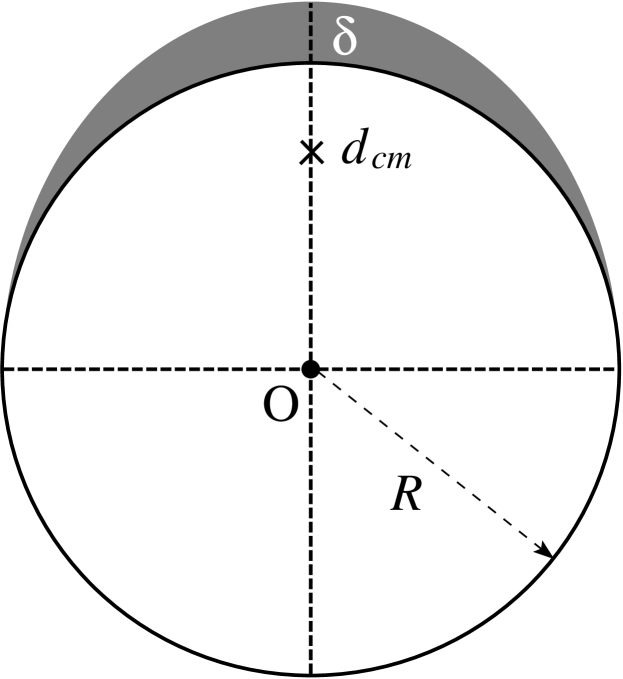
Figure 4: Schematic cross-section (not to scale) of the “egg-shell” model for a Janus particle. The white disk of radius $R$ depicts the spherical core of catalytically inactive material, while the lens-like region (dark gray area) depicts the catalyst; $\delta$ is the maximum thickness of the catalyst layer and $d_{cm}$ is its center of mass.

Accordingly, the mass of the catalyst, i.e., of the active material, within the lens-shaped layer is given by

$$m_{a}=\frac{2\pi}{3}\delta R^{2}\rho_{a}\,,$$ (18)

where $\rho_{a}$ is the mass density of the catalyst. The center of mass of the layer is located on the symmetry axis at a distance $d_{cm}=\frac{3}{4}\left(R+\frac{1}{2}\,\delta\right)\approx\frac{3}{4}R$ from the center O of the sphere ¹⁰. Disregarding the very small deviation from the spherical shape (which concerns the occurrence of a torque due to buoyancy) as well as the very small displacement of the center of mass of the particle, i.e., core plus shell, from the center O of the sphere, the gravity-induced rotation of the sphere relative to its center O is approximated by that due to the weight of the catalyst layer applied at $d_{cm}$. Therefore, the dimensionless force $\mathcal{F}$ and torque $\mathcal{T}$ (Eqs. (16d) and (16e)) are given by

$$\mathcal{F}=\frac{1}{9}\,\frac{2R^{2}(\rho_{s}-\rho)g}{\mu\,|\mathbf{U}_{ph}^{(fs)}|}\left[1+\frac{\delta}{2R}\frac{\rho_{a}-\rho}{\rho_{s}-\rho}\right]=:\frac{1}{9}F\,,$$ (19a)

and

$$\mathcal{T}=\frac{1}{12}\frac{\rho_{a}g}{\mu\,|\mathbf{U}_{ph}^{(fs)}|}R\delta=:\frac{1}{12}T\,,$$ (19b)

where $\rho_{s}$ denotes the mass density of the spherical core material. We emphasize that $T$ depends on geometrical parameters and on the density of the active material (catalyst), but not on the density of the spherical core. Accordingly, as noted in the Introduction, the torque due to gravity, i.e., the gyrotactic response of the particle, is generically relevant for Janus particles, irrespective of the kind of material the core is made of.

With these quantities, the model for chemically active, gyrotactic (bottom heavy) Janus particles near a planar, no-slip wall is complete, and we can proceed to study the dynamics.

4 Results and discussion

The trajectory of a particle, starting from an initial configuration $h(\tau=0)=h_{0}$ and $\theta(\tau=0)=\theta_{0}$, is calculated by integrating the equations of motion in Eq. (3), using a procedure which follows closely the methodology used in Refs. 23, 15, and 41. The functions $\mathbf{u}^{(1,0)}(h,\theta)$, $\mathbf{u}^{(0,1)}(h,\theta)$, $\bm{\omega}^{(1,0)}(h,\theta)$, $\bm{\omega}^{(0,1)}(h,\theta)$, and $\mathbb{M}(h)$ are evaluated on a grid of values $h_{i}$ spanning the range $1.02\leq h\leq 10$ and (at each $h_{i}$) a grid of values $\theta_{j}$ spanning the range $0\leq\theta\leq\pi$. The results are stored as five tables of values. (As noted in the section on the model and theory, this calculation has to be done only once.) The grid $\{h_{i}\}$ is nonuniform: a dense grid (small step $\Delta h=0.01$) is used for $1.02\lesssim h\lesssim 1.2$, and then the density of evaluation points is gradually decreased towards $\Delta h=0.1$ for $h>5$. The lower cut-off is due to (i) the assumptions underlying the model, e.g., that of a boundary layer (mapped onto the phoretic slip) being much thinner than the other length-scales in the problem, cease to hold; and (ii) for very small values of $h$, the computational cost of an accurate calculation of the translational and rotational velocities by the BEM becomes prohibitive. Accordingly, trajectories which reach points with $h\leq 1.02$ are classified as “crashing-into-the-wall” events. For a set of parameters $(F,T,\beta)$ and for a choice of the model activity (i.e., the expression $\mathcal{U}(\beta)$), the corresponding linear combination of the stored five tables (see Eq. (3)) is constructed; the right hand side (rhs) of Eq. (3) can then be evaluated for any pair $(h,\theta)$ by interpolation, and for any initial condition $1.02<h_{0}<10$ and $0\leq\theta_{0}\leq\pi$ the trajectory $\{h(\tau),\theta(\tau)\}$ follows upon numerical integration by using the Euler scheme with suitably small (near the wall) or large (far from the wall) time steps. In the space $(h,\theta)$ the dynamics is most conveniently visualized in the form of phase portraits, i.e., generalized flow fields, of the trajectories, starting from various initial conditions $(h_{0},\theta_{0})$.

4.1 Phase portraits of dynamics

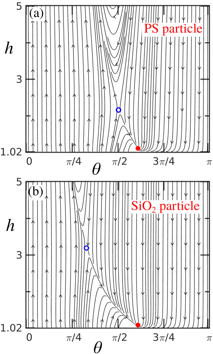
Figure 5: Phase portraits illustrating the dynamics of a chemically active Janus particle in the vicinity of the floor. The results correspond to the model activity “constant flux”, $b_{c}<0$, with the parameters $(F,T,\beta)$ given by (a) (1.2,0.62,0.5) and (b) (7.6,0.31,0.5); the red dots indicate the location of the corresponding “sliding state” attractor, while the open blue symbols indicate the location of an unstable, stationary saddle point. The first triplet could correspond to, e.g., a spherical Janus particle of radius $R=1.5~{}\mathrm{\mu m}$, made out of a PS core and a Pt film of $\delta=7~{}\mathrm{nm}$, moving with $|\mathbf{U}_{ph}^{(fs)}|=4~{}\mathrm{\mu m/s}$ (see Eqs. (19) and the discussion below); the second may be the case of, e.g., a spherical Janus particle of radius $R=1.5~{}\mathrm{\mu m}$, made out of a SiO₂ core and a Pt film of $\delta=7~{}\mathrm{nm}$, moving with $|\mathbf{U}_{ph}^{(fs)}|=8~{}\mathrm{\mu m/s}$. Note that only the region $h\leq 5$ is shown, both for reasons of clarity and because for $h>5$ the dynamics is basically that of a particle in the bulk.

An example of such phase portraits is shown in Fig. 5 for Janus particles with the model chemical activity “constant flux”, $b_{c}<0$, and distinct triplets $(F,T,\beta)$ near the “floor” (i.e., for $\mathbf{g}\cdot\mathbf{e}_{z}<0$). In both cases, for the dynamics one finds an attractor fixed point $(h^{*},\theta^{*})$, marked by the red dots in Figs. 5(a) and (b). The trajectories converge towards the attractor fixed points of the dynamics, i.e., $dh/d\tau=0$ and $d\theta/d\tau=0$ at $(h^{*},\theta^{*})$. The simultaneous vanishing of those derivatives tells that the height of the particle and its orientation with respect to the wall become constant in time; accordingly, the rhs of the third part of Eq. (3) becomes constant, too, i.e., the $y$-component of the velocity turns time-independent. Therefore, these are identified as steady states of sliding along the wall. The phase portraits also illustrate all the other generic types of trajectories observed in the study of the dynamics of a Janus particle: “crashing-into-the-wall” (see, e.g., the trajectories approaching the wall in the region $\theta>3\pi/4$), “reflection” from the wall (see, e.g., the trajectories at the center top of Fig. 5(a)), as well as “escape” from the wall (e.g., the trajectories in the region $\theta<\pi/4$).

We recall that for small magnitudes of $F$ and $T$ (Eq. 19) the dynamics is expected to be similar to that exhibited by the model particle in a gravitationless environment. However, in the case $(F,T)=(0,0)$ the distinction between floor and ceiling disappears. Thus, if sliding states occur at one wall, they should occur also at the other one. If this happens, the sliding states should also occur, simultaneously, for $(F,T)$ being close to $(0,0)$, although the topologies of the corresponding phase portraits will start to differ as the location $(F,T)$ moves further away from $(0,0)$. The expectation of the simultaneous occurrence of sliding states at the floor and at the ceiling for small values of $F$ and $T$ can be directly tested in the context of the same model with “constant flux” chemical activity and $b_{c}<0$. For this case it is known that sliding states, solely due to phoresis, may occur ²³.

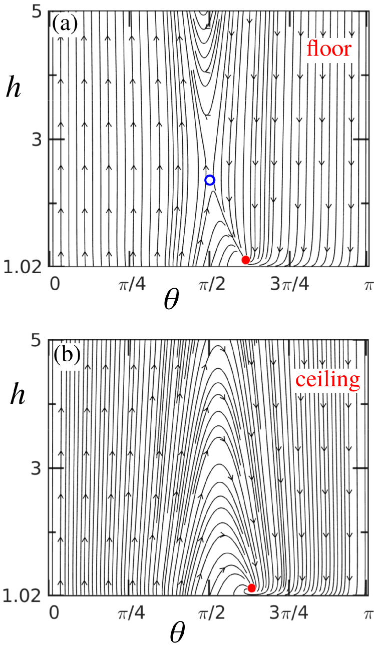
Figure 6: Phase portraits for a model Janus particle with “constant flux” chemical activity, $b_{c}<0$, and the parameters $(F,T,\beta)=(0.86,0.49,0.5)$ in the vicinity of (a) the floor and (b) the ceiling; the red dots indicate the location of the corresponding “sliding state” attractor, while the open blue symbol in panel (a) indicates the location of a saddle point. Note that only the region $h\leq 5$ is shown, both for reasons of clarity and because for $h>5$ the dynamics is basically that of a particle in the bulk.

As shown in Fig. 6, this is indeed the case: for small, but non-zero, $F=0.86$ and $T=0.49$, sliding states are possible at both walls for the same value of $\beta$, i.e., the exact same particle and with the same activity, i.e., the same value of $U_{ph}^{(fs)}$. Although the corresponding configurations (height $h^{*}$ and orientation $\theta^{*}$) of the sliding states at the floor and at the ceiling are very similar, the topologies of the phase portraits are clearly distinct. Moreover, their corresponding basins of attractions, i.e., the set of initial conditions for which the trajectories converge to the fixed point, have different extents.

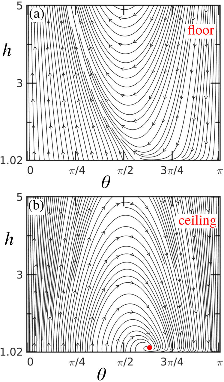
Figure 7: Phase portraits for a model Janus particle with “constant flux” chemical activity, $b_{c}<0$, and the parameters $(F,T,\beta)=(0.1,4,0.9)$ in the vicinity of (a) the floor and (b) the ceiling; the red dot indicates the location of the corresponding “sliding state” attractor. Note that only the region $h\leq 5$ is shown, both for reasons of clarity and because for $h>5$ the dynamics is basically that of a particle in the bulk.

As noted in the Introduction, another scenario reported in experimental studies is that Janus particles, which – owing to a sufficiently large chemical activity – move upwards (against gravity, eventually after a lift-off from the floor), upon collision with the ceiling attain a sliding state along it ^{10, 25, 11, 12}. As shown in Fig. 7, this scenario can be captured also by the model Janus particle with a “constant flux” chemical activity and $b_{c}<0$.

4.2 Theoretical state-diagrams

The results discussed above highlight the rich behavior exhibited by the dynamics of the model Janus particle, as well as the fact that the model captures (qualitatively) the types of sliding states and the set-up (floor or ceiling) encountered in experimental studies.Additionally, for suitable choices of $(F,T,\beta)$, for both models the dynamics exhibits also the previously reported “hovering” states, both at the floor and the ceiling. These states have proven to be difficult to detect experimentally, with only one report of observation seemingly compatible with such a state ¹⁹. We only succinctly discuss them in the SI Sec. B, and focus the discussion here on the sliding states. Moreover, the feature of co-existing sliding states at the floor and the ceiling ^{11, 28} is also predicted to occur for certain values of the parameters, too (see Fig. 6). (We note that, as discussed below, similar results can be obtained by using the “variable flux” model with $b_{c}<0$, but, obviously, for other values of the triplet $(F,T,\beta)$.) It is therefore important to understand how the occurrence of the (experimentally observable) sliding states at the ceiling or at the floor (or both, or none) depends on the parameters of the model, i.e., the sign of $b_{c}$ and the values of $(F,T,\beta)$. This understanding would provide the means for a comparison with the corresponding experimental results. Accordingly, we proceed by constructing “state-diagrams”, which illustrate various domains in the parameter space (constrained by the range of experimental relevance, as discussed below). They correspond to each of the possible scenarios for the occurrence of sliding states.

In spite of the significant reduction in complexity provided by the representation as a linear superposition of solutions corresponding to three basic problems, it remains a challenge to study in detail a dependence on four parameters. Thus it is desirable to reduce the number of parameters, as well as the ranges within which the remaining ones are allowed to vary. For our system this reduction is feasible, based on the results of previously published studies, as well as based on the fact that some of the quantities involved in the definition of $F$ and $T$ are known material parameters.

The available studies of Pt/PS or Pt/SiO₂ Janus colloids immersed in aqueous H₂O₂ solutions report the motion to be the one with the catalyst at the back (see, e.g., Refs. 8, 10, 25, 15, 16, 9, 13). The majority of these reports deal with particles presumably sliding along a horizontal wall, for which the velocity parallel to the wall is solely due to the chemical activity component (the sedimentation cannot contribute along that direction); Refs. 10, 25, 11 report also lift-off and upward motion, which can be due only to the chemical activity component. Accordingly, in the context of our phoretic motion models one infers that (see also Fig. 3) $\mathbf{U}_{ph}^{(fs)}\cdot\mathbf{p}<0$. Based on the expression of $\mathbf{U}_{ph}^{(fs)}$ (Eq. (14)) the most plausible case^{23, 15, 16} is that the phoretic mobility of the active (catalyst-covered) area is negative, i.e., $b_{c}<0$ (which corresponds to a repulsive effective interaction between the solute molecules and the particle) and $\mathcal{U}(\beta)>0$. Therefore, in Eqs. (16d) and (16e) and (3)

$$b_{c}/|b_{c}|=-1\,,~{}\mathrm{and}~{}|\mathcal{U}(\beta)|=\mathcal{U}(\beta)\,,$$ (20)

while from Eq. (15) it follows that the parameter $\beta$ is restricted by the lower bound

$$-1<\beta\,,~{}\textrm{constant flux,}$$

$$-3.4\lesssim\beta\,,~{}\textrm{variable flux.}$$ (21)

As far as an upper bound for the range of $\beta$ is concerned, for both models we shall explore values of $\beta$ as large as $\beta\simeq 1$, i.e., the same value of the phoretic mobility across the whole surface. For this value of $\beta$, the Janus particle does not exhibit phoretic rotations in response to distortions of the chemical field ^{23, 22}. Accordingly, this choice of the upper bound limits the study to the case that the rotation solely due to the distortion of the chemical field is such as to turn the active cap of the particle away from the wall ²³. With reference to the left panel in Fig. 1, for a bottom heavy particle this situation promotes the emergence of sliding states – upon approach to the wall – with an orientation of the cap somewhat tilted away from the wall. This seems to be the situation in the experiments with Pt/PS and Pt/SiO₂ particles ^{15, 9, 25}.

Turning to the parameters $F$ and $T$, the mass densities of the core materials, of the catalyst, and of the solution, as well as the viscosity of the solution, are known. For the system of interest here, the particle parameters are $\rho_{s}\approx 1050$ kg/m³ (PS) or 2196 kg/m³ (amorphous SiO₂), and $\rho_{a}\approx 21450$ kg/m³ (Pt catalyst), while for the aqueous solution $\rho\approx 1000$ kg/m³ and $\mu\approx 9\times 10^{-4}$ Pa$\cdot$s (at 25 ^∘C). The radius of the particles is usually in the range $0.5~{}\mathrm{\mu m}\leq R\leq 3~{}\mathrm{\mu m}$. The parameter $\delta$ (i.e., the thickness of the catalyst layer at the pole of the Janus particle) is taken to be equal to the thickness reported by the thin-film deposition procedure, i.e., $\delta=\delta_{rep}$. Guided by the typical values reported in the literature ^{13, 9, 15, 10, 8}, here we take $\delta$ in the range $7~{}\textrm{nm}\leq\delta\leq 30~{}\textrm{nm}$.

On the other hand, the dependence of $F$ and $T$ on the phoretic velocity $|\mathbf{U}_{ph}^{(fs)}|$ in unbounded solution is a point of concern, because this velocity is difficult to determine experimentally. Here, we simply assume, as done previously^{15, 16, 19}, that $|\mathbf{U}_{ph}^{(fs)}|$ is of the same order as the velocity observed in experiments for particles sliding along the wall. This interpretation is also supported by the results (reported in Ref. 10) for the upward migration of Pt/PS particles (slightly density mismatched with the solution), which is similar to the values of the velocity along the wall. Furthermore, the theoretical predictions for the velocity $U_{y}$ along the wall (see Fig. 3 and Eq. (3)) for the sliding states shown in Figs. 5 - 7, as well as for a few other tested cases, have shown that it deviates by a factor $0.8-1.1$ from the corresponding $|\mathbf{U}_{ph}^{(fs)}|$. Based on these arguments, we assume that the value of the phoretic velocity in unbounded solution lies in the range $1~{}\mathrm{\mu m/s}\leq|\mathbf{U}_{ph}^{(fs)}|\leq 10~{}\mathrm{\mu m/s}$, as usually reported by experimental studies. Here we note that much larger velocities, of the order of tens (up to a hundred) of $\mathrm{\mu m/s}$, have been reported in Ref. 26 for Pt/PS spherical Janus particles in aqueous peroxide solutions of moderate concentrations. These values are very different from all the other reports in the literature (for seemingly similar systems)^{9, 8, 28, 11, 10, 25}. Accordingly, we leave aside this exceptional, rather than typical case.

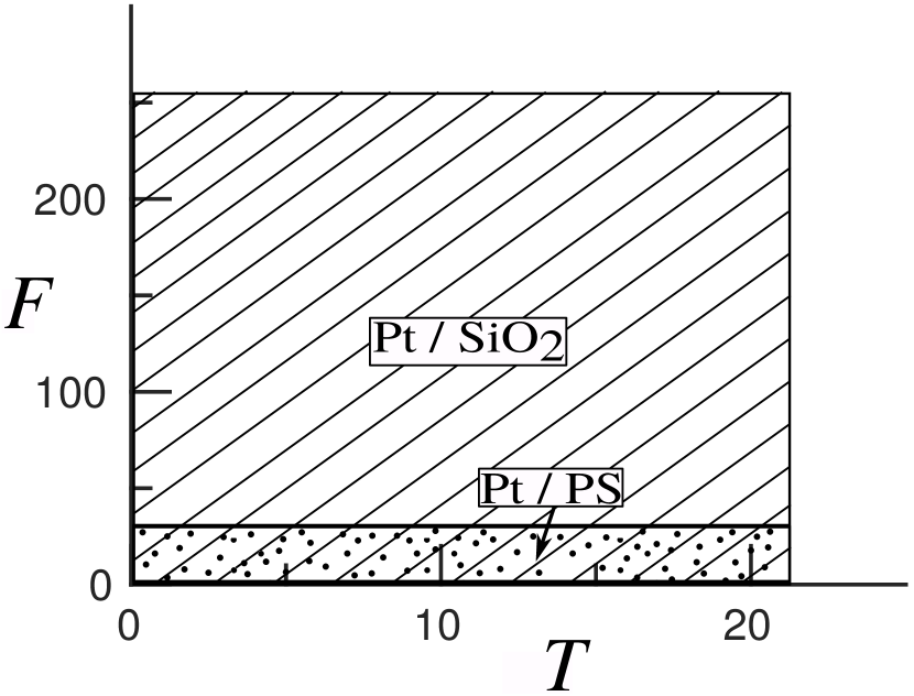
Figure 8: The subspace of the parameter space $(F,T)$ (see Eq. (19)) which is relevant for experiments with Pt/PS and Pt/SiO₂ chemically active Janus particles immersed in aqueous H₂O₂ solutions (see the main text).

Collecting all pieces, one arrives at the experimentally relevant ranges for the parameters $F$ and $T$ as

$$0.11\lesssim F\lesssim 254$$ (22)

$$\mathrm{and}$$

$$0.09\lesssim T\lesssim 21\,.$$ (23)

This parameter subspace is shown in Fig. 8, where the relatively small subset corresponding to the particles with PS core (for which there are more experimental reports available) is also indicated.

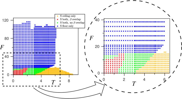
Figure 9: State-diagram of sliding states (S) for the constant flux model and $b_{c}<0$. The white region corresponds to the absence of sliding states at either wall, within the range of values of $\beta$ analyzed here (see the main text). The label “$\beta$ overlap” and “no $\beta$ overlap” refers to scenario (v) and (iv), respectively, described in the main text.

The study of the dynamics as a function of the parameters $F$, $T$, and $\beta$, constrained to the ranges outlined above, has been carried out for each of the two model chemical activities as follows. A grid of pairs $(F,T)$, spanning the whole relevant domain (Eqs. (22) and (23)), is selected; for each pair $(F,T)$, phase portraits as the ones above are generated – for both the ceiling and the floor cases – at a number of values of $\beta$, in steps of 0.1 starting from the minimum within the corresponding range (Eq. (4.2)). These phase portraits are analyzed with regard to the occurrence of sliding states; the outcome is used to classify the behavior at $(F,T)$ as follows (see also SI Sec. A): (i) no sliding states occur, irrespective of $\beta$ and the kind of wall (i.e., floor or ceiling); (ii) sliding states occur for a subset of values of $\beta$, but only at the floor; (iii) sliding states occur, for a subset of values of $\beta$, but only at the ceiling; (iv) sliding states occur both at the floor and at the ceiling, but the subsets of values of $\beta$ for the floor and for the ceiling do not overlap; (v) sliding states occur both at the floor and at the ceiling, and the intersection of the subsets of values of $\beta$ for the floor and for the ceiling is non-void. (This listing includes all scenarios encountered in the theoretical analysis.)

The resulting classes, i.e., $(F,T)$ and one of the five cases above, provide a “state-diagram” of the sliding steady-states of the dynamics. The state-diagrams for the constant-flux (“cf”) and the variable-flux (“vf”) models, which are the main results of the present study, are shown in Figs. 9 and 10, respectively.

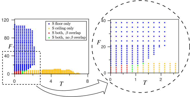
Figure 10: State-diagram of sliding states (S) for the variable flux model and $b_{c}<0$. The white region corresponds to the absence of sliding states at either wall, within the range of values of $\beta$ analyzed here (see the main text). The label “$\beta$ overlap” and “no $\beta$ overlap” refers to scenario (v) and (iv), respectively, described in the main text.

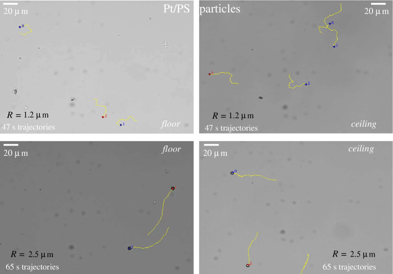
Figure 11: Tracked trajectories of Pt/PS Janus particles in sliding states at the floor (left column) and at the ceiling (right column), for particles of size $R=1.2~{}\mathrm{\mu m}$ (top row) and $2.5~{}\mathrm{\mu m}$ (bottom row), respectively. The progression of the trajectory is from its free end towards the end with the particle attached. Note the difference in duration of the trajectory between the top and bottom rows. The labels near the particles are added by the tracking software; their sole purpose is that of indexing the various tracked trajectories.

At the quasi-quantitative level, these state-diagrams reveal significant differences between the behaviors emerging from the two models. Although qualitatively they cannot be discriminated, because both capture all possible outcomes (i)-(v), the domains corresponding to these states differ significantly; in particular, compared with model “cf”, model “vf” predicts a significantly narrowed range of values of $T$ for which sliding states at the floor may occur (the blue region), as well as a significant shrinking of the domain where coexisting sliding states may occur (the red region).

4.3 Comparison with experimental results

By comparing Figs. 9 and 10 with Fig. 8, one infers that Pt/PS Janus particles are the best candidates for the experimental validation of coexisting sliding states because their parameter $F$ is typically within the range where such state are expected to occur. This is a somewhat fortunate situation, in view of the fact that a number of experimental studies employing Pt/PS Janus particles are available ^{9, 11, 28, 25} and, as noted above, in some of them the presence of motile particles at the top walls was noted ^{11, 28}. On the other hand, for Pt/SiO₂ Janus particles the mass density mismatch between the core material and the solution is large, and thus $F$ attains larger values. Accordingly, such particles may be used to explore the region of coexisting sliding states only if they are small and if their self-propulsion is sufficiently strong. In practice, the latter condition might be difficult to achieve because it requires a relatively large rate of solute (O₂) production and the formation of O₂ bubbles in the solution becomes significant. Guided by these observations, our experiments have been focused on the case of Pt/PS Janus particles; but, as discussed in the experimental section, Pt/SiO₂ Janus particles of two different sizes have been studied, too. Further motivation for carrying out these experiments follows from the fact that the number of independent studies of such particles is quite small yet, and that there are large discrepancies in the values of the velocity reported for presumably similar experiments performed by different groups. For example, for Pt/PS particles of radius 1 $\mathrm{\mu m}$ in 10% H₂O₂ aqueous solution, Ref. 11 reports a velocity of 15 - 20 $\mathrm{\mu m/s}$, and Ref. 28 quotes a velocity slightly less than 4 $\mathrm{\mu m/s}$, while the only differences between these particles consists of the thickness of the Pt layer (5 nm vs 10 nm) and of the method of depositing Pt. This difference by a factor of 4-5, which directly transfers into the magnitudes of $F$ and $T$, can cause significant differences concerning the region in the state diagram which the point should be attributed to (see also, c.f., Fig. 13).

Both the smaller ($R=1.2~{}\mathrm{\mu m}$) and the larger ($R=2.5~{}\mathrm{\mu m}$) Pt/PS Janus particles, which self-propel within the $3\%$ H₂O₂ aqueous solution, exhibit sliding states at both the ceiling and the floor (see the videos SI.V1 to SI.V4), so that these states coexist. This finding provides a welcome reassurance that the phenomenon is indeed experimentally observable and robust with respect to variations of the parameters. As illustrated by the tracked trajectories shown in Fig. 11 (see also the videos SI.V1 to SI.V4), the sliding motions at the ceiling and at the floor are very similar. (We note that the recordings cover different time intervals. Accordingly, the duration of the trajectories in the top panels in Fig. 11 is different from that of the trajectories in the bottom panels in Fig. 11). Therefore, as noted in the experimental section, the velocities of the particles for the sliding states are de facto independent of the location (ceiling or floor) and of the size of the particles. Furthermore, in the videos SI.V4 and SI.V5 (see the SI) one clearly observes that particles arrive from the bulk and start to slide along the ceiling (see the particles labeled as “2” in each of these videos, and the description of the videos in the SI Sec. D). This observation confirms that the presence of the particles in sliding states at the ceiling is the result of the dynamics and not some artifact such as the attachment of the particles when the ceiling (i.e., a glass slide) is placed at the top of the experimental cell. Both the observed phenomenon and the value of the velocity (comparable at the floor and at the ceiling) of the particles are commensurate with those noted in Ref. 28 for a similar concentration of the aqueous H₂O₂ solution.

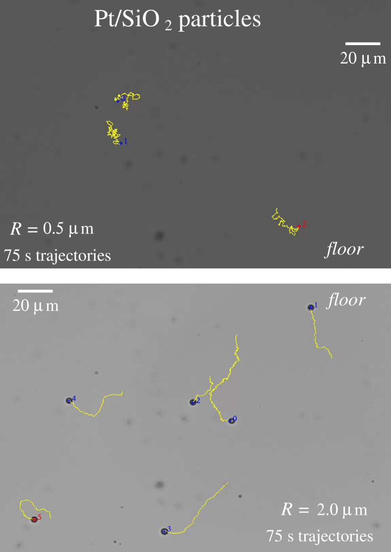
Figure 12: Tracked trajectories of Pt/SiO₂ in sliding states at the floor, for particles of sizes $R=0.5~{}\mathrm{\mu m}$ (top panel) and $2.0~{}\mathrm{\mu m}$ (bottom panel), respectively. The progression of the trajectory is from its free end towards the end with the particle attached. There is a significant winding of the trajectories of the smaller particles compared to the ones of the larger particles. The labels near the particles are added by the tracking software; their sole purpose is that of indexing the various tracked trajectories.

source	particle type	$R$ ($\mu m$)	$\delta$ ($nm$)	sliding location	$U_{ph}^{(fs)}$ ($\mu m/s$)	$F$	$T$	symbol	location check
									model $cf$	model $vf$
this work	$\rm{Pt/PS}$	1.2	9	$(f,c)$	1.6	2.5	1.6		$\checkmark$	$\times$
this work	$\rm{Pt/PS}$	2.5	9	$(f,c)$	1.6	7.4	3.3		$\times$	$\times$
this work	$\rm{Pt/SiO_{2}}$	0.5	9	$(f)$	2.1	3.6	0.5		$\times$	$\times$
this work	$\rm{Pt/SiO_{2}}$	2	9	$(f)$	1.4	77.3	3		$\checkmark$	$\times$
Ref. 15	$\rm{Pt/SiO_{2}}$	1	7	$(f)$	6	4.6	0.27	$\bf{\medtriangleleft}$	$\times$	$\times$
Ref. 15	$\rm{Pt/SiO_{2}}$	2.5	7	$(f)$	6	27.8	0.7	$\medtriangleleft$	$\checkmark$	$\checkmark$
Ref. 11	$\rm{Pt/PS}$	1	5	$(f,c)$	17	0.13	0.07	$\medcircle$	$\checkmark$	$\checkmark$
Ref. 9	$\rm{Pt/PS}$	2.5	7	$(f)$	2.5	4.3	1.6	$\medtriangleright$	$\checkmark$	$\times$
Ref. 9	$\rm{Pt/PS}$	2.5	7	$(f)$	9	1.2	0.45	$\medtriangleright$	$\times$	$\times$
Ref. 28	$\rm{Pt/PS}$	1	7	$(f,c)$	1	2.6	1.6	$\meddiamond$	$\checkmark$	$\times$
Ref. 28	$\rm{Pt/PS}$	1	7	$(f,c)$	3.75	0.7	0.4	$\meddiamond$	$\checkmark$	$\checkmark$
Ref. 28	$\rm{Pt/PS}$	1.5	7	$(f,c)$	1	4.8	2.5	$\meddiamond$	$\times$	$\times$
Ref. 28	$\rm{Pt/PS}$	1.5	7	$(f,c)$	2.5	1.9	1.0	$\meddiamond$	$\checkmark$	$\checkmark$
Ref. 28	$\rm{Pt/PS}$	2.5	7	$(f,c)$	1	10.7	4.1	$\meddiamond$	$\times$	$\times$
Ref. 25	$\rm{Pt/PS}$	3.5	10	$(c)$	5.4	3.9	1.5	$\medsquare$	$\checkmark$	$\checkmark$

Table 1: The values of the parameters corresponding to the experimentally studied particles indicated by symbols in Fig. 13. The letters f and c in the fifth column refer to sliding states located near the floor or the ceiling, respectively. The tick “$\checkmark$” indicates that the corresponding point belongs to a compatible domain of the theoretically predicted state-diagram for the corresponding model (i.e., $cf$ (constant flux) or $vf$ (variable flux), respectively), whereas the symbol “$\times$” indicates that it does not belong to them.

In contrast, at the same concentration of the H₂O₂ aqueous solution, in the case of the Pt/SiO₂ Janus particles we have observed sliding states only at the floor, even when using smaller particles ($R=0.5~{}\mathrm{\mu m}$). The typical motion in a sliding state at the floor is illustrated, in the form of tracked trajectories, in Fig. 12 (see also the videos SI.V6 and SI.V7 in the SI). The difference in speed between the particles of different sizes (see the experimental section), with the smaller particles moving faster (see also Ref. 56), is not easily noticeable via visual inspection.

Finally, we note that while, as discussed above, the models capture all the relevant, experimentally observable phenomenology, it is interesting to analyze whether these considerations hold even on a more quantitative level. For example, a simple check is provided by locating the points $(T,F)$ corresponding to the experiments (the present ones and from, e.g., Refs. 9, 11, 28, 25) within the state-diagrams and by checking the compatibility between the observed state(s) and the model-predicted state. This is illustrated in Fig. 13, where we show the points, corresponding to our estimates $(T,F)$ for the various experimental realizations, on top of the region of the state-diagram to which they belong to (see Table 1).

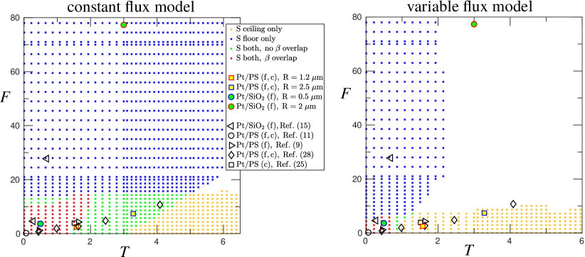
Figure 13: Comparison of the experimental results (symbols, see the legend valid for both panels) with the corresponding theoretical predictions of their state (in terms of sliding state occurrence). The indices $c$ and $f$ refer to the location (ceiling or floor) where the experimental observation was made. The theoretical predictions shown in the two panels are the corresponding sub-regions indicated in Figs. 9 and 10. The label “$\beta$ overlap” and “no $\beta$ overlap” refers to scenario (v) and (iv), respectively, described in the main text.

It is apparent that, at the quantitative level, neither of the two models captures the complete set of experimental data points as a whole. However – recalling the simplicity of the models employed in the study – the agreement is actually reasonably good. For example, concerning the constant flux model the predictions are in agreement with the experimental observations in nine out of the fifteen cases studied here (see Table 1). (It has to be noticed that in three of these cases observations have been reported either only at the floor or only at the ceiling. Accordingly, only a somewhat weak agreement can be claimed because, in the absence of observations at both locations, it cannot be inferred whether the experimental point belongs to one of the regions without coexistence (blue, yellow, or green), or to the one with coexistence (red).) Furthermore, from the point of view of these state-diagrams, it may eventually be inferred that the “cf” model seems to provide a closer match of the experimental observations than the “vf” model does. However, before drawing conclusions such as that one or the other (or both) activity models are too simple (i.e., they miss essential physical ingredients), one should recall that very crude models and approximations have been made concerning the estimates of the parameters $\delta$ and $|\mathbf{U}_{ph}^{(fs)}|$. (In addition, the latter is further affected by conflicting values reported from various experiments.) Taking the case of Pt/PS particles and the coexisting sliding states as an example, one observes that increasing the estimates of $\delta$ by a factor of, e.g., 1.5 is sufficient to shift one of the points corresponding to the current experiments (filled squares) and some of those in Ref. 28 (open diamonds) out of the red colored region of the state-diagram corresponding to the constant flux model. This sensitivity concerning the precise value of $\delta$ is heightened further by noting that its interpretation is connected with a very simple geometrical model for the catalyst film, the reliability of which has only recently been been investigated experimentally ⁵⁷. Accordingly, while the results of the present analysis are encouraging, we think that they are insufficient for drawing strong conclusions, such as claims of quantitative agreement or discriminating resolution between distinct models of chemical activity.

5 Conclusions

We have theoretically investigated the dynamics of chemically active, gyrotactic Janus particles near walls. The particles are located either above the floor or below the ceiling of the sample. We have focused on the emergence of wall-bound steady sliding states. For this analysis, we have used two distinct models corresponding to a constant (cf) or a variable (vf) flux of the chemical emission of the particle. The theoretical analysis has been complemented by experiments conducted with Pt/PS and Pt/SiO₂ Janus particles immersed in aqueous H₂O₂ solutions, which have been set up such as to optimize the eventual occurrence of sliding states simultaneously at the floor and the ceiling. We have shown that, for both choices of the chemical activity, the models capture all the phenomenology of sliding states observed in the experiments, including that of coexistence of ceiling- and floor-sliding states as noted in previous experimental studies and confirmed by the present Pt/PS experiments.

For each of the two models, the various scenarios of sliding states at the ceiling and the floor have been studied as functions of the parameters $(F,T,\beta)$ that determine the dynamics (see Eq. (3)). The results concerning the sliding state occurrence have been summarized in terms of “state-diagrams” in the $(T,F)$ plane. In particular, the occurrence of sliding state coexistence at the ceiling and the floor, or the occurrence of only one of the two states, at points $(T,F)$ where both states are allowed but for different values of $\beta$, sets very strong bounds on the otherwise hard to measure (or estimate) ratio $\beta$ of the phoretic mobilities for self-phoretic Janus particles (Eq. (13)).

The structure of these “state-diagrams” seems to be sufficiently different to allow one, eventually, to discriminate between models with different choices of the chemical activity (or ruling out both of them), provided quantitative comparisons can be made with the experiments. A first attempt of such a comparison with the results of present experiments, as well as with those of previously published experimental studies, shows a reasonable quasi-quantitative agreement with the theoretical predictions. However, we caution that this finding could be a spurious feature emerging from the inherent uncertainties in estimating the phoretic velocity in unbounded solutions and in modeling the distribution of catalyst at the surface of the particles. In particular for Pt/PS particles, the relevant parameters characterizing them depend very sensitively on these two quantities. This uncertainty, together with the significant differences between the velocities reported in the available experimental investigations for seemingly similar particles and solutions, highlights the necessity of additional, systematic, and thorough experimental studies. The state-diagrams derived here, and the underlying analysis of the role of the various parameters and of the assumptions concerning the geometry of the problem, should prove to be useful in guiding such investigations. The results of such studies may then eventually validate and discriminate between the various models of the self-motility mechanism.

Video recordings, showing the motion, within a 3% (v/v) aqueous H₂O₂ solution, of Pt/PS particles at the floor and at the ceiling, and of Pt/SiO₂ particles at the floor, are provided as Supplementary Information (SI). Additionally, the SI contains details concerning the procedure to classify the “state scenario” at a point $(F,T)$ (SI Sec. A), a discussion of the observation of “hovering” steady-states at the floor and at the ceiling (SI Sec. B), a glossary and list of symbols (SI Sec. C), and a brief description of the video files (SI Sec. D).

Notes
The authors declare that there is no competing financial interest.

I.K. and Z.J. acknowledge support by the National Science Foundation under the award number CBET-1705565.

Supplementary Information

Appendix A Classifying the “state scenario” at a point $(F,T)$

As explained in the main text, at a given point $(F,T)$ in the parameter space, $\beta$ is varied within the corresponding range of values, and the phase portraits are analyzed with respect to the occurrence of sliding states. These results are algorithmically summarized and interpreted in order to determine the corresponding scenario, in terms of sliding states, as schematically depicted in Fig. A.1. (Note that here, for reasons of clarity, we show only a smaller subset of values of $\beta$.)

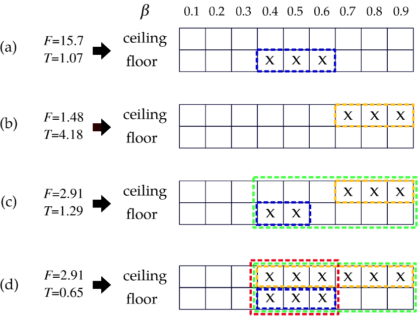
Figure A.1: Schematic illustration of the interpretation of the “states” in terms of sliding states at the floor and the ceiling for various values of $\beta$ (here, for reasons of clarity, only the range $0.1\leq\beta\leq 0.9$ is shown). The various panels correspond to the specific points $(F,T)=$ (15.7,1.07) (a); (1.48,4.18) (b); (2.91,1.29) (c); and (2.91,0.65) (d), which are located in the four distinct regions in Fig. 9.

In brief: each value $\beta$ gets allocated an entry in the ceiling and floor rows. If the corresponding phase portrait reveals a sliding state, the entry is “checked” (illustrated in the figure by “x”), otherwise it is left unchecked. In the next step, if there are checked entries in the floor (ceiling) row, the corresponding row is marked for a sliding state as “blue” (floor) or “gold” (ceiling). If only one of the colors is present, as in the panels (a) and (b) in Fig. A.1, or if no color is present, the procedure ends and the point $(F,T)$ is classified as belonging to the scenarios “sliding states only at the ceiling (floor)” or “no sliding state”, respectively. If both colors are present, the color is set to “green” (see panels (c) and (d) in Fig. A.1); if there is overlap between the checked entries in the top and in the bottom rows (panel (d)), the color is further changed to “red”, otherwise it is kept unchanged. The state is then classified as belonging to the scenarios “sliding states at both walls, but for non-overlapping subsets of $\beta$” (green) or “coexisting sliding states” (red), respectively.

Appendix B Steady states of “hovering”

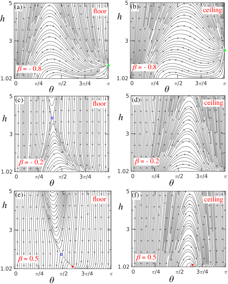
Figure B.1: Phase portraits for a model heavy, gyrotactic Janus particle with constant flux chemical activity, $b_{c}<0$, and the parameters $F=4,\;T=1$, near the floor (left column)] and near the ceiling (right column) for values $\beta=-0.8\;[(a),(b)],\;-0.2\;[(c),(d)]\;\text{and}\;0.5\;[(e),(f)]$. The green markers denote hovering states, while the red markers denote sliding states; also the locations of saddle points are indicated by the open blue symbols in (c) and (e). Note that only the region $h\leq 5$ is shown, both for reasons of clarity and because for $h>5$ the dynamics is basically that of a particle in the bulk.

As noted in the main text, it is known that the dynamics of a self-phoretic Janus particle near a wall exhibits an additional type of steady-state, the so called “hovering” state²³: the particle is at rest at a height $h^{*}$ above the wall and with an orientation $\theta^{*}=\pi$, while still pumping the fluid. Although there is only indirect experimental evidence for such states ¹⁹, it is nevertheless interesting to understand if these states, which for, e.g., heavy, gyrotactic particles, are favored at one wall (e.g., the ceiling), but disfavored at the other (the floor), can occur for the model particles studied here.

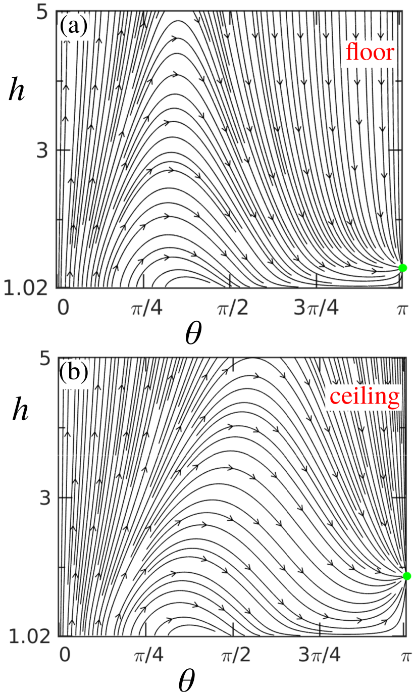
Figure B.2: Phase portraits for a model heavy, gyrotactic Janus particle with variable flux chemical activity, $b_{c}<0$, and the parameters $(F=4,\;T=1,\;\beta=-2.5)$ near the floor (a) and near the ceiling (b). In both cases, the green markers denote hovering states. Note that only the region $h\leq 5$ is shown, both for reasons of clarity and because for $h>5$ the dynamics is basically that of a particle in the bulk.

As shown in Fig. B.1, this is indeed the case here: similar to the case of the sliding states discussed in the main text, hovering states can also occur, both at the floor and at the ceiling, and coexistence of floor- and ceiling-hovering is possible. As illustrated in that figure, a model heavy, gyrotactic Janus particle with constant flux chemical activity, $b_{c}<0$, and parameters $(F=4,\;T=1)$ exhibits sliding states for sufficiently large, positive values of $\beta$ (see Figs. B.1 (e) and (f)). However, at sufficiently large, negative values of $\beta$ one observes hovering states (see Figs. B.1 (a) and (b)). In both the floor and the ceiling case, the transition from hovering to sliding attractors is not continuous, at least within the limits of the numerical accuracy and of the constraint $h>1.02$ imposed on the model. However, this transition involves a range of values for the parameter $\beta$ (see Figs. B.1 (c) and (d)) within which steady motion of the particle is possible only in the bulk (far from the wall). Concerning the location of the hovering state, one notices that, in the case of coexistence of such states, the hovering occurs further away from the wall at the ceiling as compared to the floor. This follows from the fact that the particle is, due to the choice of the parameters, heavy (i.e., it tends to sediment near the floor). Accordingly, at the ceiling the gravity-induced velocity opposes the approach to the wall due to the phoretic velocity.

Hovering steady-states — as well as the co-existence of such states — occur also in the case of the variable flux chemical activity. This situation is illustrated by Fig. B.2 which corresponds to the same parameters $(F,T)$ as above and to $b_{c}<0$, but $\beta=-2.5$. As noted in the discussion in the main text, the two models are qualitatively equivalent concerning the type of steady-state scenarios.

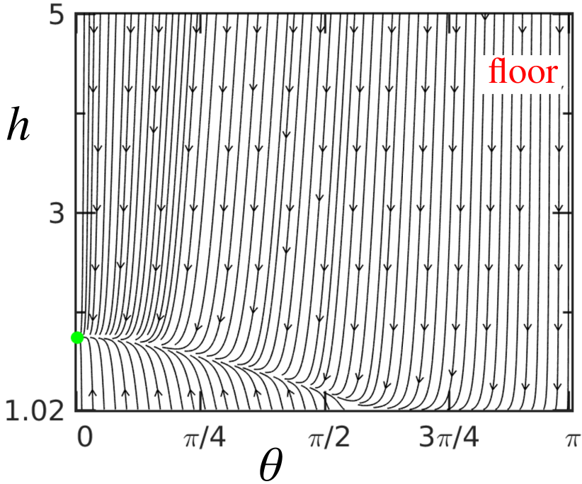
Figure B.3: Phase portrait for a model heavy, gyrotactic Janus particle with constant flux chemical activity, $b_{c}<0$, and the parameters $(F=25,\;T=2,\;\beta=0.9)$ near the floor. The green marker indicates the cap-down ($\theta=0$) hovering state. Note that only the region $h\leq 5$ is shown, both for reasons of clarity and because for $h>5$ the dynamics is basically that of a particle in the bulk.

Figure B.4: Five possible phase portraits for a model heavy, gyrotactic Janus particle with constant flux chemical activity, $b_{c}<0$, and the parameters $(F=20,\;T=1)$, when moving near the floor. Upon varying the ratio $\beta$ of the phoretic mobilities, the following scenarios emerge (illustrated in the panels within the dashed circles). For $0.68\lesssim\beta<1$ (cyan region), a cap-down ($\theta=0$, stable (s) hovering (H) state (filled green symbol) emerges. Decreasing $\beta$ further, in the range $0.37\lesssim\beta\lesssim 0.68$ (orange region) one observes coexistence between the cap-down stable hovering state (filled green symbol) with a stable sliding (S) state (filled red symbol), separated by an (unstable, stationary) saddle point (sp, open blue symbol). The sliding state disappears once $\beta\simeq 0.37$, and for $0.25\lesssim\beta\lesssim 0.37$ (magenta region) the cap-down stable hovering state (filled green symbol) coexists with the saddle point (open blue symbol), the location of which is shifting towards $\theta=0$ as $\beta$ decreases. At $\beta\simeq 0.25$ the hovering point and the saddle point collide, and for $-0.7\lesssim\beta\lesssim 0.27$ (green region) the phase portraits exhibit only an unstable (u) cap-down hovering state (open green symbol). Finally, at $\beta\simeq-0.7$ an additional, stable, cap-up ($\theta=\pi$) hovering state emerges (filled green symbol), and for $-1\lesssim\beta\lesssim-0.7$ (blue region) coexistence of this state with the unstable cap-down state (open green symbol) is observed.

The hovering states discussed above are configurations with the active cap oriented away from the wall (i.e., $\theta^{*}=\pi$), similar to those discussed in Ref. 23 in the absence of gravity. However, for the gyrotactic, bottom heavy, sedimenting active Janus spheres discussed here a new type of hovering state exists at the floor, with the active cap oriented towards the wall (i.e., $\theta^{*}=0$), as shown in Fig. B.3. This state is easy to grasp intuitively, in that it occurs if at a certain height $h^{*}$ above the wall the sedimentation velocity is exactly balanced by the self-propulsion (both of them depending on $h$ and, for $\theta=0$, having opposite signs).

Finally, we note that for a sedimenting, gyrotactic, chemically active Janus particle the dynamic behavior at the floor is significantly enriched compared to the case, studied theoretically in Refs. 23 and 41, in which the effects of gravity (sedimentation and gyrotaxis) are disregarded. This enrichment occurs not only in terms of the appearance of a new type of steady state, i.e., the “cap down” hovering noted above, but, as shown in Fig. B.4, also in terms of coexisting steady states of sliding and hovering at the floor corresponding to bi-stability. For example, for a Janus particle with parameters $(F,\;T)=(20,1)$ and $b_{c}<0$, for $\beta<-0.7$ one observes coexistence of a stable cap-up ($\theta^{*}=\pi$) hovering state with an unstable cap-down ($\theta^{*}=0$) one. Upon increasing $\beta$ above the value $\beta\simeq-0.7$, the stable hovering point disappears; once $\beta>0.25$, the unstable cap-down hovering state splits into a stable cap-down hovering one and a saddle-point. From $\beta>0.37$, a sliding state also occurs, and for $0.37\lesssim\beta\lesssim 0.68$ one observes coexistence of a sliding state (cap slightly tilted away from the wall, $\theta^{*}>\pi/2$) with a stable cap-up hovering state ($\theta^{*}=0$), separated by a saddle point. Finally, for $\beta>0.68$ only the stable cap-up hovering state is present in the dynamics.

An exhaustive investigation of this very rich dynamics is beyond the scope of this study and is left for future analysis.

Appendix C Glossary and list of symbols

In order to facilitate the reading of the paper, here we summarize the mathematical symbols and abbreviations used throughout the main text of this study.

symbols	details
R	particle radius (m) (before Eq. (1))
$U_{0}$	characteristic particle velocity (m/s) (Eq. (14))
$t_{0}$	characteristic time (s) (Eq. (12))
$F_{0}$	characteristic force (N) (Eq. (16d))
$T_{0}$	characteristic torque (N $\times$ m) (Eq. (16e))
$\mathbf{U}$	particle translational velocity (m/s) (Eq. (7a))
$t$	time elapsed (s) (Eq. 12)
${\mathbf{F}}_{\textit{g}}$	gravitational force (N) (Eq. (16d))
${\mathbf{T}}_{\textit{g}}$	gravitational torque (N $\times$ m) (Eq. (16e))
$h$	dimensionless height of the particle centroid from the wall (Fig. 3)
$D$	diffusion coefficient of the solute molecules (m2/s) (Eq. (2a))
$Pe$	dimensionless Péclet number (page 6, before Eq. (1))
$\mathbf{r}$	position vector of any point in the solution (m) (Eq. (1))
${\mathbf{r}}_{s}$	position vector at a point on the particle surface (m) (Eq. (2a))
$c(\mathbf{r})$	solute number density at a point in the solution (m-3) (Eq. (1))
$\mathcal{Q}$	total rate of solute production (m${}^{-2}\times$ s-1) (Eq. (1))
$\mathcal{S}$	particle surface (Fig. 1)
$\mathbf{p}$	unit vector along the particle symmetry axis, towards the active pole (Fig. 3)
$q({\mathbf{r}}_{s})$	chemical activity function (Eq. (3))
$\mathbf{e}_{x,y,z}$	unit vector along $x,y,z$ direction (Fig. 3)
$\mathbf{n}$	unit vector denoting the outer normal of the wall (Fig. 3)
${\mathbf{v}}_{s}$	phoretic slip velocity (m/s) (Eq. (4))
$b({\mathbf{r}}_{s})$	surface mobility of the particle (m5/s) (Eq. (4))
Re	dimensionless Reynolds number (between Eqs. (5) and (6))
${\mathbf{v}}({\mathbf{r}})$	velocity field (m/s) (Eq. (6))
$P(\mathbf{r})$	fluid pressure field (Pa) (after Eq. (6))
$\mathbb{M}$	mobility matrix (Eq. (11))
$m_{i,j}$	elements of the mobility matrix (Eq. (16))
$\mathcal{U}(\beta)$	a prefactor depending on the activity-based-model (Eq. (14))
$\mathbf{u}$	dimensionless particle translational velocity (Eq. (16a))
$F$	dimensionless apparent weight of the particle (Eq. (19a))
$T$	dimensionless gravitactic torque on the particle (Eq. (19b))
$\mathcal{F}$	$F/9$ (Eq. (16d))
$\mathcal{T}$	$T/12$ (Eq. (16e))
$m_{a}$	mass of the deposited catalyst layer (kg) (Eq. (18))
g	acceleration due to gravity (m2/s) (Fig. 1)
$\hat{\mathcal{I}}$	identity tensor (after Eq. (4))

Greek	details
$\mu$	dynamic viscosity of the suspending fluid (Pa $\times$ sec) (before Eq. (6))
$\Omega_{0}$	characteristic particle rotational velocity (s-1) (before Eq. (13))
$\mathbf{\Omega}$	particle rotational velocity (s-1) (Eq. (7a))
$\theta$	orientation angle of the particle (Fig. 3)
$\delta$	maximum thickness of the catalyst layer (m) (Fig. 4)
$\chi$	angle between ${\mathbf{r}}_{s}$ and director $\mathbf{p}$ (Fig. 3)
$\nabla$	gradient operator (Eq. (2a))
$\nabla_{||}$	surface gradient operator (Eq. (4))
$\bm{\hat{\sigma}}$	stress tensor (N/m2) (Eq. (6))
$\beta$	ratio of inert and active phoretic mobilities (Eq. (13))
$\bm{\omega}$	dimensionless particle rotational velocity (Eq. (16b))
$\tau$	dimensionless time (Eq. (3))
$\rho_{a}$	mass density of the catalyst (kg/m3) (Eq. (19a))
$\rho_{s}$	mass density of the inert core of the particle (kg/m3) (Eq. (19a))
$\rho$	mass density of the hydrogen peroxide solution (kg/m3) (Eq. (19a))
subscripts	details
$rep$	reported value
$cf$	constant flux
$vf$	variable flux
$c$	active cap
$i$	inert portion of the particle surface
$x,y,z$	x,y,z Cartesian coordinates
$w$	wall (floor or ceiling)
$g$	gravitational contribution
$ph$	phoretic contribution
$O$	position of the hcenter of mass of the particle
superscripts	details
(1,0)	$(b_{c},b_{i})=(1,0)$
(0,1)	$(b_{c},b_{i})=(0,1)$
($fs$)	free space

Appendix D Description of the video files of Pt/PS and Pt/SiO₂ active Janus particles

Videos of Pt/PS and Pt/SiO₂ active Janus particles:

• The video files SI.V1 to SI.V5 illustrate the motion of platinum-capped (Pt thickness $\delta=8.5$ nm) polystyrene (Pt/PS) Janus particles of diameters 2.4 and 5 $\mu$m, respectively, in 3% (v/v) aqueous H₂O₂ solution both at the ceiling and at the floor.

• The video files SI.V6 and SI.V7 illustrate the motion of platinum-capped (Pt thickness $\delta=8.5$ nm) silica (Pt/SiO₂) Janus particles of diameters 1 and 4 $\mu$m, respectively, in 3% (v/v) aqueous H₂O₂ solution at the floor. The video recording was carried out with a u-eye 2240c camera at a rate of 10 frames per second (fps). The yellow curves show tracked trajectories of particles (tracking has been performed using the ImageJ software and an in-house Matlab script).

Video-file details:

VideoSI.V1: Motion of three Pt/PS Janus particles of 2.4 $\mu$m diameter, at the floor (file name: VideoSI.V1_2.4um_ptps_3H2O2_bottom_20x.m4v).

VideoSI.V2: Motion of four Pt/PS Janus particles of 2.4 $\mu$m diameter, at the ceiling (file name: VideoSI.V2_2.4um_ptps_3H2O2_top_20x.webm).

VideoSI.V3: Motion of two Pt/PS Janus particles of 5 $\mu$m diameter, at the floor (file name: VideoSI.V3_5um_ptps_3H2O2_bottom_20x.webm).

VideoSI.V4: Motion of three Pt/PS Janus particles of 5 $\mu$m diameter, at the ceiling. The third particle arrives at the ceiling at time t = 14 s (file name: VideoSI.V4_5um_ptps_3H2O2_top_20x.webm).

VideoSI.V5: Motion of two Pt/PS Janus particles of 2.4 $\mu$m diameter, at the ceiling. The third particle arrives at the ceiling at time t = 30 s (file name: VideoSI.V5_2.4um_ptps_3H2O2_top_20x.webm).

VideoSI.V6: Motion of three Pt/SiO₂ Janus particles of diameter 1 $\mu$m, at the floor (file name: VideoSI.V6_1um_ptSiO2_3H2O2_bottom_20x.m4v).

VideoSI.V7: Motion of six Pt/SiO₂ Janus particles of diameter 1 $\mu$m, at the floor (file name: VideoSI.V7_4um_ptSiO2_3H2O2_bottom_20x.webm).

References

- Paxton et al. 2004 Paxton, W. F.; Kistler, K. C.; Olmeda, C. C.; Sen, A.; St. Angelo, S. K.; Cao, Y. Y.; Mallouk, T. E.; Lammert, P. E.; Crespi, V. H. Catalytic nanomotors: autonomous movement of striped nanorods. J. Am. Chem. Soc. 2004, 126, 13424
- Fournier-Bidoz et al. 2005 Fournier-Bidoz, S.; Arsenault, A. C.; Manners, I.; Ozin, G. A. Synthetic self-propelled nanorotors. Chem. Commun. 2005, 0, 441
- Ebbens and Howse 2010 Ebbens, S. J.; Howse, J. R. In pursuit of propulsion at the nanoscale. Soft Matter 2010, 6, 726
- Moran and Posner 2016 Moran, J. L.; Posner, J. D. Phoretic self-propulsion. Ann. Rev. Fluid Mech. 2016, 49, 511
- Sánchez et al. 2015 Sánchez, S.; Soler, L.; Katuri, J. Chemically Powered Micro- and Nanomotors. Angew. Chem. Int. Ed. 2015, 54, 1414
- Hong et al. 2010 Hong, Y.; Velegol, D.; Chaturvedi, N.; Sen, A. Biomimetic behavior of synthetic particles: from microscopic randomness to macroscopic control. Phys. Chem. Chem. Phys. 2010, 12, 1423
- 7 The deposition of the main, catalytic material is sometimes preceded by that of an ultrathin layer of a material, which facilitates the adhesion of the catalyst, such as Ti on polystyrene before depositing Pt (see, e.g., Ref. 9).
- Howse et al. 2007 Howse, J. R.; Jones, R. A. L.; Ryan, A. J.; Gough, T.; Vafabakhsh, R.; Golestanian, R. Self-motile colloidal particles: from directed propulsion to random walk. Phys. Rev. Lett. 2007, 99, 048102
- Baraban et al. 2012 Baraban, L.; Tasinkevych, M.; Popescu, M. N.; Sánchez, S.; Dietrich, S.; Schmidt, O. G. Transport of cargo by catalytic Janus micro-motors. Soft Matter 2012, 8, 48
- Campbell and Ebbens 2013 Campbell, A. I.; Ebbens, S. J. Gravitaxis in spherical Janus swimming devices. Langmuir 2013, 29, 14066
- Brown and Poon 2014 Brown, A.; Poon, W. Ionic effects in self-propelled Pt-coated Janus swimmers. Soft Matter 2014, 10, 4016
- Takatori et al. 2016 Takatori, S.; De Dier, R.; Vermant, J.; Brady, J. Acoustic trapping of active matter. Nature Commun. 2016, 7, 10694
- Jalilvand et al. 2018 Jalilvand, Z.; Pawar, A.; Kretzschmar, I. Experimental study of the motion of patchy particle swimmers near a wall. Langmuir 2018, 34, 15593
- Wang et al. 2015 Wang, X.; In, M.; Blanc, C.; Nobili, M.; Stocco, A. Enhanced active motion of Janus colloids at the water surface. Soft Matter 2015, 11, 7376
- Simmchen et al. 2016 Simmchen, J.; Katuri, J.; Uspal, W. E.; Popescu, M. N.; Tasinkevych, M.; Sánchez, S. Topographical pathways guide chemical microswimmers. Nature Commun. 2016, 7, 10598
- Katuri et al. 2018 Katuri, J.; Uspal, W. E.; Simmchen, J.; Miguel López, A.; Sánchez, S. Cross-stream migration of active particles. Sci. Adv. 2018, 4, eaao1755
- Maggi et al. 2016 Maggi, C.; Simmchen, J.; Saglimbeni, F.; Katuri, J.; Dipalo, M.; De Angelis, F.; Sanchez, S.; Di Leonardo, R. Self-Assembly of Micromachining Systems Powered by Janus Micromotors. Small 2016, 12, 446
- Katuri et al. 2018 Katuri, J.; Caballero, D.; Voituriez, R.; Samitier, J.; Sanchez, S. Directed Flow of Micromotors through Alignment Interactions with Micropatterned Ratchets. ACS Nano 2018, 12, 7282
- Singh et al. 2018 Singh, D.; Uspal, W.; Popescu, M.; Wilson, L.; Fischer, P. Photo-gravitactic microswimmers. Adv. Func. Mat. 2018, 28, 1706660
- Singh et al. 2017 Singh, D. P.; Choudhury, U.; Fischer, P.; Mark, A. G. Non-Equilibrium Assembly of Light-Activated Colloidal Mixtures. Adv. Mater. 2017, 29, 1701328
- Aubret et al. 2017 Aubret, A.; Ramananarivo, S.; Palacci, J. Eppur si muove, and yet it moves: Patchy (phoretic) swimmers. Curr. Op. Colloid Interf. Sci. 2017, 30, 81
- Popescu et al. 2018 Popescu, M. N.; Uspal, W. E.; Domínguez, A.; Dietrich, S. Effective interactions between chemically active colloids and interfaces. Acc. Chem. Res. 2018, 51, 2991
- Uspal et al. 2015 Uspal, W. E.; Popescu, M. N.; Dietrich, S.; Tasinkevych, M. Self-propulsion of a catalytically active particle near a planar wall: from reflection to sliding and hovering. Soft Matter 2015, 11, 434
- Volpe et al. 2011 Volpe, G.; Buttinoni, I.; Vogt, D.; Kümmerer, H. J.; Bechinger, C. Microswimmers in patterned environments. Soft Matter 2011, 7, 8810
- Campbell et al. 2019 Campbell, A.; Ebbens, S. J.; Illien, P.; Golestanian, R. Experimental observation of flow fields around active Janus spheres. Nature Commun. 2019, 10, 1
- Dietrich et al. 2017 Dietrich, K.; Renggli, D.; Zanini, M.; Volpe, G.; Buttinoni, I.; Isa, L. Two-dimensional nature of the active Brownian motion of catalytic microswimmers at solid and liquid interfaces. New J. Phys. 2017, 19, 065008
- Palacios et al. 2019 Palacios, L. S.; Katuri, J.; Pagonabarraga, I.; Sánchez, S. Guidance of active particles at liquid - liquid interfaces near surfaces. Soft Matter 2019, 15, 6581
- Das et al. 2015 Das, S.; Garg, A.; Campbell, A. I.; Howse, J. R.; Sen, A.; Velegol, D.; Golestanian, R.; Ebbens, S. J. Boundaries can steer active Janus spheres. Nature Commun. 2015, 6, 8999
- Uspal et al. 2015 Uspal, W. E.; Popescu, M. N.; Dietrich, S.; Tasinkevych, M. Rheotaxis of spherical active particles near a planar wall. Soft Matter 2015, 11, 6613
- Uspal et al. 2018 Uspal, W. E.; Popescu, M. N.; Tasinkevych, M.; Dietrich, S. Shape-dependent guidance of active Janus particles by chemically patterned surfaces. New J. Phys. 2018, 20, 015013
- Domínguez et al. 2016 Domínguez, A.; Malgaretti, P.; Popescu, M. N.; Dietrich, S. Effective interaction between active colloids and fluid interfaces induced by Marangoni flows. Phys. Rev. Lett. 2016, 116, 078301
- Enculescu and Stark 2011 Enculescu, M.; Stark, H. Active colloidal suspensions exhibit polar order under gravity. Phys. Rev. Lett. 2011, 107, 058301
- Ginot et al. 2018 Ginot, F.; Solon, A.; Kafri, Y.; Ybert, C.; Tailleur, J.; Cottin-Bizonne, C. Sedimentation of self-propelled Janus colloids: polarization and pressure. New J. Phys. 2018, 20, 115001
- ten Hagen et al. 2014 ten Hagen, B.; Kümmel, F.; Wittkowski, R.; Takagi, D.; Löwen, H.; Bechinger, C. Gravitaxis of asymmetric self-propelled colloidal particles. Nature Commun. 2014, 5, 4829
- Drescher et al. 2009 Drescher, K.; Leptos, K. C.; Tuval, I.; Ishikawa, T.; Pedley, T. J.; Goldstein, R. E. Dancing Volvox: hydrodynamic bound states of swimming algae. Phys. Rev. Lett. 2009, 102, 168101
- Shen and Lintuvuori 2019 Shen, Z.; Lintuvuori, J. S. Gravity induced formation of spinners and polar order of spherical microswimmers on a surface. Phys. Rev. Fluids 2019, 4, 123101
- Brumley and Pedley 2019 Brumley, D. R.; Pedley, T. J. Stability of arrays of bottom-heavy spherical squirmers. Phys. Rev. Fluids 2019, 4, 053102
- Kuhr et al. 2017 Kuhr, J.-T.; Blaschke, J.; Rühle, F.; Stark, H. Collective sedimentation of squirmers under gravity. Soft Matter 2017, 13, 7548
- Rühle et al. 2018 Rühle, F.; Blaschke, J.; Kuhr, J.-T.; Stark, H. Gravity-induced dynamics of a squirmer microswimmer in wall proximity. New J. Phys. 2018, 20, 025003
- Mozaffari et al. 2016 Mozaffari, A.; Sharifi-Mood, N.; Koplik, J.; Maldarelli, C. Self-diffusiophoretic colloidal propulsion near a solid boundary. Phys. Fluids 2016, 28, 053107
- Bayati et al. 2019 Bayati, P.; Popescu, M. N.; Uspal, W. E.; Dietrich, S.; Najafi, A. Dynamics near planar walls for various model self-phoretic particles. Soft Matter 2019, 15, 5644
- Popescu et al. 2016 Popescu, M. N.; Uspal, W. E.; Dietrich, S. Self-diffusiophoresis of chemically active colloids. Eur. Phys. J. Special Topics 2016, 225, 2189
- Golestanian et al. 2007 Golestanian, R.; Liverpool, T.; Ajdari, A. Designing phoretic micro- and nano-swimmers. New J. Phys. 2007, 9, 126
- Ebbens et al. 2014 Ebbens, S.; Gregory, D. A.; Dunderdale, G.; Howse, J. R.; Ibrahim, Y.; Liverpool, T. B.; Golestanian, R. Electrokinetic Effects in Catalytic Pt-Insulator Janus Swimmers. EPL 2014, 106, 58003
- Popescu et al. 2018 Popescu, M. N.; Uspal, W. E.; Eskandari, Z.; Tasinkevych, M.; Dietrich, S. Effective squirmer models for self-phoretic chemically active spherical colloids. Eur. Phys. J. E 2018, 41, 145
- Ibrahim et al. 2017 Ibrahim, Y.; Golestanian, R.; Liverpool, T. B. Multiple phoretic mechanisms in the self-propulsion of a Pt-insulator Janus swimmer. J. Fluid Mech. 2017, 828, 318
- Prevo and Velev 2004 Prevo, B. G.; Velev, O. D. Controlled, Rapid Deposition of Structured Coatings from Micro- and Nanoparticle Suspensions. Langmuir 2004, 20, 2099
- Pozrikidis 2002 Pozrikidis, C. A Practical Guide to Boundary Element Methods with the Software Library BEMLIB; CRC Press: Boca Raton, 2002
- Anderson 1989 Anderson, J. L. Colloid transport by interfacial forces. Ann. Rev. Fluid Mech. 1989, 21, 61
- Bechinger et al. 2016 Bechinger, C.; Di Leonardo, R.; Löwen, H.; Reichhardt, C.; Volpe, G.; Volpe, G. Active particles in complex and crowded environments. Rev. Mod. Phys. 2016, 88, 045006
- Happel and Brenner 1973 Happel, J.; Brenner, H. Low Reynolds number hydrodynamics; Noordhoff Int. Pub.: Leyden, The Netherlands, 1973
- Michelin and Lauga 2014 Michelin, S.; Lauga, E. Phoretic self-propulsion at finite Péclet numbers. J. Fluid Mech. 2014, 747, 572
- Rashidi et al. arXiv:1903.09127 (2019 Rashidi, A.; Razavi, S.; Wirth, C. Influence of cap weight on the motion of a Janus particle very near a wall. arXiv:1903.09127 (2019)
- 54 Additionally, for suitable choices of , for both models the dynamics exhibits also the previously reported “hovering” states, both at the floor and the ceiling. These states have proven to be difficult to detect experimentally, with only one report of observation seemingly compatible with such a state 19. We only succinctly discuss them in the SI Sec. B, and focus the discussion here on the sliding states.
- 55 Here we note that much larger velocities, of the order of tens (up to a hundred) of , have been reported in Ref. 26 for Pt/PS spherical Janus particles in aqueous peroxide solutions of moderate concentrations. These values are very different from all the other reports in the literature (for seemingly similar systems)9, 8, 28, 11, 10, 25. Accordingly, we leave aside this exceptional, rather than typical case.
- Ebbens et al. 2012 Ebbens, S.; Tu, M. H.; Howse, J. R.; Golestanian, R. Size dependence of the propulsion velocity for catalytic Janus-sphere swimmers. Phys. Rev. E 2012, 85, 020401(R)
- Rashidi et al. 2018 Rashidi, A.; Issa, M. W.; Martin, I. T.; Avishai, A.; Razavi, S.; Wirth, C. L. Local measurement of Janus particle cap thickness. ACS App. Mater. & Interf. 2018, 10, 30925