$e^{T}$ 1.0: an open source electronic structure program with emphasis on coupled cluster and multilevel methods

Abstract

The $e^{T}$ program is an open source electronic structure package with emphasis on coupled cluster and multilevel methods. It includes efficient spin adapted implementations of ground and excited singlet states, as well as equation of motion oscillator strengths, for CCS, CC2, CCSD, and CC3. Furthermore, $e^{T}$ provides unique capabilities such as multilevel Hartree-Fock and multilevel CC2, real-time propagation for CCS and CCSD, and efficient CC3 oscillator strengths. With a coupled cluster code based on an efficient Cholesky decomposition algorithm for the electronic repulsion integrals, $e^{T}$ has similar advantages as codes using density fitting, but with strict error control. Here we present the main features of the program and demonstrate its performance through example calculations. Because of its availability, performance, and unique capabilities, we expect $e^{T}$ to become a valuable resource to the electronic structure community.

I Introduction

During the last five decades, a wide variety of models and algorithms have been developed within the field of electronic structure theory and many program packages are now available to the community.(Helgaker, Jørgensen, and Olsen, 2014) Programs with extensive coupled cluster functionality include CFOUR,(Stanton et al., 2010) Dalton,(Aidas et al., 2014) GAMESS,(Gordon and Schmidt, 2005) Molcas,(Aquilante et al., 2016) Molpro,(Werner et al., 2012) NWChem,(Valiev et al., 2010) ORCA,(Neese, 2012) Psi4,(Parrish et al., 2017) QChem,(Shao et al., 2015) and TURBOMOLE.(Furche et al., 2014) Although these are all general purpose quantum chemistry programs, each code is particularly feature rich or efficient in specific areas. For instance, a large variety of response properties(Helgaker et al., 2012) have been implemented in Dalton, CFOUR is particularly suited for gradients(Koch et al., 1990; Stanton, 1993) and geometry optimization, and QChem is leading in equation of motion(Stanton and Bartlett, 1993; Krylov, 2008) (EOM) features. However, due to the long history of many of these programs, it can be challenging to modify and optimize existing features or to integrate new methods and algorithms.

In 2016, we began developing a coupled cluster code based on Cholesky decomposed electron repulsion integrals.(Beebe and Linderberg, 1977; Koch, Sánchez de Merás, and Pedersen, 2003) While starting anew, we have drawn inspiration from Dalton(Aidas et al., 2014) and used it extensively for testing purposes. Our goal is to create an efficient, flexible, and easily extendable foundation upon which coupled cluster methods and features—both established and new—can be developed. That code has now evolved beyond a coupled cluster code into an electronic structure program. It is named $e^{T}$ after the expression for the coupled cluster ground state wave function,(Coester and Kümmel, 1960)

$$|\Psi\rangle=e^{T}|\mathrm{R}\rangle,$$ (1)

and released as an open source program licensed under the GNU General Public License 3 (GPL 3.0).

The first version of $e^{T}$ offers an optimized Hartree-Fock (HF) code and a wide range of standard coupled cluster methods. It includes the most efficient published implementations of Cholesky decomposition of the electron repulsion integrals(Folkestad, Kjønstad, and Koch, 2019) and of coupled cluster singles, doubles and perturbative triples(Koch et al., 1997; Myhre and Koch, 2016) (CC3). Furthermore, $e^{T}$ features the first released implementations of multilevel HF(Sæther et al., 2017) (MLHF), multilevel coupled cluster singles and perturbative doubles(Myhre, Sánchez de Merás, and Koch, 2014; Folkestad and Koch, 2019) (MLCC2), and explicitly time-dependent coupled cluster singles (TD-CCS) and singles and doubles (TD-CCSD) theory. All coupled cluster models can be used in quantum mechanics/molecular mechanicsWarshel and Karplus (1972); Levitt and Warshel (1975) (QM/MM) calculations, or be combined with the polarizable continuum model(Tomasi, Mennucci, and Cammi, 2005; Mennucci, 2012) (PCM).

$e^{T}$ is primarily written in modern Fortran, using the Fortran 2008 standard. The current version of the code is interfaced to two external libraries: Libint 2Valeev (2017) for the atomic orbital integrals and PCMSolver 1.2Di Remigio et al. (2019a) for PCM embedding. In addition, $e^{T}$ applies the runtest library(Bast, 2018) for testing and a CMake module from autocmake(Bast, Di Remigio, and Juselius, 2020) to locate and configure BLAS and LAPACK.

With the introduction of the 2003 and 2008 standards, Fortran has become an object oriented programming language. We have exploited this to make $e^{T}$ modular, readable, and easy to extend. Throughout the program, we use OpenMP(OMP, ) to parallelize computationally intensive loops. In order to preserve code quality, extensive code review and enforcement of a consistent standard has been prioritized from the outset. While this requires extra effort from both developers and maintainers, it pays dividends in code readability and flexibility.

II Program features

II.1 Coupled cluster methods

The $e^{T}$ program features all standard coupled cluster methods up to perturbative triples: singles (CCS), singles with perturbative doubles(Christiansen, Koch, and Jørgensen, 1995) (CC2), singles and doubles(Purvis and Bartlett, 1982) (CCSD), singles and doubles with non-iterative perturbative triples(Raghavachari et al., 1989) (CCSD(T)), and singles and doubles with perturbative triples(Koch et al., 1997) (CC3). At the CCSD(T) level of theory, only ground state energies can be computed. For all other methods, efficient spin adapted implementations of ground and excited singlet states are available. Moreover, dipole and quadrupole moments, as well as EOM oscillator strengths, can be calculated. Equation of motion polarizabilities are available at the CCS, CC2, and CCSD levels of theory.

A number of algorithms are implemented to solve the coupled cluster equations. For linear and eigenvalue equations, we have implemented the Davidson method.Davidson (1975) This algorithm is used to solve the ground state multiplier equations, response equations, and excited state equations. To handle nonlinear coupled cluster equations, we have implemented algorithms that use direct inversion of the iterative subspace(Pulay, 1982, 1980) (DIIS) to accelerate convergence. The ground state amplitude equations can be solved using DIIS combined with the standard(Helgaker, Jørgensen, and Olsen, 2014; Scuseria, Lee, and Schaefer, 1986) quasi-Newton algorithm or exact Newton-Raphson. We also use a DIIS-accelerated algorithm(Hättig and Weigend, 2000) for the nonlinear excited state equations in CC2 and CC3. Our implementation of DIIS incorporates the option to use the related conjugate residual with optimal trial vectors(Ziółkowski et al., 2008; Ettenhuber and Jørgensen, 2015) (CROP) method for acceleration. For the nonperturbative coupled cluster methods, the asymmetric Lanczos algorithm is also available.(Lanczos, 1950; Coriani et al., 2012)

The time-dependent coupled cluster equations can be explicitly solved for CCS and CCSD(Koch and Jørgensen, 1990; Pedersen and Kvaal, 2019) using Euler, Runge-Kutta 4 (RK4), or Gauss-Legendre (GL2, GL4, GL6) integrators. This requires implementations of the amplitude and multiplier equations with complex variables. Any number of classical electromagnetic pulses can be specified in the length gauge, assuming that the dipole approximation is valid. A modified version of the fast Fourier transform library FFTPACK 5.1(Swarztrauber, 1984) is used to extract frequency domain information.

II.2 Cholesky decomposition for the electronic repulsion integrals

Cholesky decomposition is an efficient method to obtain a compact factorization of the rank deficient electron repulsion integral matrix.(Beebe and Linderberg, 1977; Koch, Sánchez de Merás, and Pedersen, 2003; Aquilante et al., 2011) All post HF methods in $e^{T}$rely on the Cholesky vectors to construct the electron repulsion integrals. One advantage of factorization is the reduced storage requirements; the size of the Cholesky vectors scales as $\mathcal{O}(n_{\mathrm{AO}}^{3})$ while the full integral matrix scales as $\mathcal{O}(n_{\mathrm{AO}}^{4})$. The Cholesky vectors are kept in memory when possible, but are otherwise stored on disk. Another advantage is that they allow for efficient construction and transformation of subsets of the integrals. The Cholesky decomposition in $e^{T}$ is highly efficient, consisting of a two step procedure that reduces both storage requirements and computational cost compared to earlier algorithms.(Folkestad, Kjønstad, and Koch, 2019)

II.3 Hartree-Fock

The restricted (RHF) and unrestricted HF (UHF) models are implemented in $e^{T}$. The implementations are integral direct and exploit Coloumb and exchange screening and permutation symmetry. We use a superposition of atomic densities(Van Lenthe et al., 2006) (SAD) initial guess constructed from spherically averaged UHF calculations on the constituent atoms. The Hartree-Fock equations are solved using a Roothan-Hall self-consistent field (SCF) algorithm accelerated either by DIIS or CROP. To improve the screening and reduce the number of integrals that must be evaluated, density differences are used to construct the Fock matrix.

II.4 Multilevel and multiscale methods

In MLHF, a region of the molecular system is defined as active. A set of active occupied orbitals are obtained through a restricted, partial Cholesky decomposition of an initial idempotent AO density matrix.Sánchez de Merás et al. (2010) Active virtual orbitals are obtained by constructing projected atomic orbitalsPulay (1983); Saebo and Pulay (1993) (PAOs) centered on the active atoms. The PAOs are orthonormalized through the canonical orthonormalization procedure.(Löwdin, 1970) The MLHF equations are solved using a DIIS accelerated, MO based, Roothan-Hall SCF algorithm. Only the active MOs are optimized.(Høyvik, 2019)

The most expensive step of an MLHF calculation is the construction of the inactive two electron contribution to the Fock matrix. As the inactive orbitals are frozen, it is only necessary to calculate this term once. The iterative cost in MLHF is dominated by the construction of the active two electron contribution to the Fock matrix. An additional Coulomb and exchange screening, which targets accuracy of the matrix in the active MO basis, reduces the cost. The active orbitals are localized and, consequently, elements of the AO Fock matrix which correspond to AOs distant from the active atoms will not significantly contribute to the active MO Fock matrix. This is similar to the screening used in MLHF specific Cholesky decomposition of the electron repulsion integrals.(Folkestad, Kjønstad, and Koch, 2019)

In MLCC2,(Myhre, Sánchez de Merás, and Koch, 2013, 2014; Myhre and Koch, 2016; Folkestad and Koch, 2019) an active orbital space is treated at the CC2 level of theory, while the remaining inactive orbitals are treated at the CCS level of theory. MLCC2 excitation energies are implemented in $e^{T}$. The active space is constructed using either approximated correlated natural transition orbitals,(Høyvik, Myhre, and Koch, 2017; Baudin and Kristensen, 2017) Cholesky orbitals, or Cholesky occupied orbitals and PAOs spanning the virtual space.

Frozen orbitals are implemented for all coupled cluster methods in $e^{T}$. In addition to the standard frozen core (FC) approximation, reduced space coupled cluster calculations can be performed using semi-localized orbitals. This type of calculation is suited to describe localized properties. In reduced space calculations, the occupied space is constructed from Cholesky orbitals and PAOs are used to generate the virtual space.

Two QM/MM approaches are available in $e^{T}$: electrostatic QM/MM embeddingSenn and Thiel (2009) and the polarizable QM/Fluctuating ChargeCappelli (2016) (QM/FQ) model. In the former, the QM density interacts with a set of fixed charges placed in the MM part of the system.Senn and Thiel (2009) In QM/FQ, the QM and MM parts mutually polarize. Each atom in the MM part has a charge that varies as a response to differences in atomic electronegativities and the QM potential.Cappelli (2016) These charges enter the QM Hamiltonian through a term that is nonlinear in the QM density.Lipparini, Cappelli, and Barone (2012)

PCM embedding can be used in $e^{T}$ for an implicit description of the external environment. A solute is described at the QM level and is placed in a molecule shaped cavity. The environment is described in terms of an infinite, homogeneous, continuum dielectric that mutually polarize with the QM part, as in QM/FQ.Di Remigio et al. (2019b)

In the QM/PCM and QM/FQ implementations, additional terms are only added to the Fock matrix. Additional terms, at the coupled cluster level, can also be considered.Caricato (2019); Cammi (2009); Caricato (2012); Caricato et al. (2013); Ren et al. (2019)

II.5 Spectroscopic properties and response methods

Coupled cluster is one of the most accurate methods for modelling spectroscopic properties, and both UV/Vis and X-ray absorption spectra can be modelled in $e^{T}$. Core excitations are obtained through the core valence separation (CVS) approximation.(Cederbaum, Domcke, and Schirmer, 1980) CVS is implemented as a projection(Coriani and Koch, 2015, 2016) for CCS, CC2, MLCC2, and CCSD. For CC3, amplitudes and excitation vector elements that do not contribute are not calculated. This reduces the scaling of the iterative computational cost from $\mathcal{O}(n_{\mathrm{MO}}^{7})$ to $\mathcal{O}(n_{\mathrm{MO}}^{6})$.

Intensities are obtained from EOM oscillator strengths,(Stanton and Bartlett, 1993; Krylov, 2008) which are available for CCS, CC2, CCSD, and CC3. In addition, linear response(Koch and Jørgensen, 1990) (LR) oscillator strengths can be calculated at the CCS level of theory. The asymmetric Lanczos algorithm(Lanczos, 1950; Coriani et al., 2012) can be used to directly obtain both energies and EOM oscillator strengths for CCS, CC2 and CCSD. It can also be combined with the CVS approximation.

Real-time propagation offers a nonperturbative approach to model absorption spectra. Following an initial pulse that excites the system, the dipole moment from the subsequent time evolution can be Fourier transformed to extract the excitation energies and intensities.

Valence ionization potentials are implemented for CCS, CC2, and CCSD. A bath orbital that does not interact with the system is added to the calculation. Excitation vector components not involving this orbital are projected out in an approach similar to the projection in CVS.(Coriani and Koch, 2015, 2016)

III Illustrative applications and performance tests

In this section, we will demonstrate some of the capabilities of $e^{T}$ with example calculations. Thresholds are defined as follows. Energy thresholds refer to the change in energy from the previous iteration. The maximum norm of the gradient vector is used in Hartree-Fock calculations. For coupled cluster calculations in $e^{T}$ and Dalton, residual thresholds refer to the $L^{2}$ norm of the residual vectors. Finally, the Cholesky decomposition threshold refers to the largest absolute error on the diagonal of the electron repulsion integral matrix. This threshold gives an upper bound to the error of all matrix elements. Coupled cluster calculations were performed with either Cholesky vectors or electron repulsion integrals in memory. All geometries are available from Ref. 72.

III.1 Coupled cluster methods

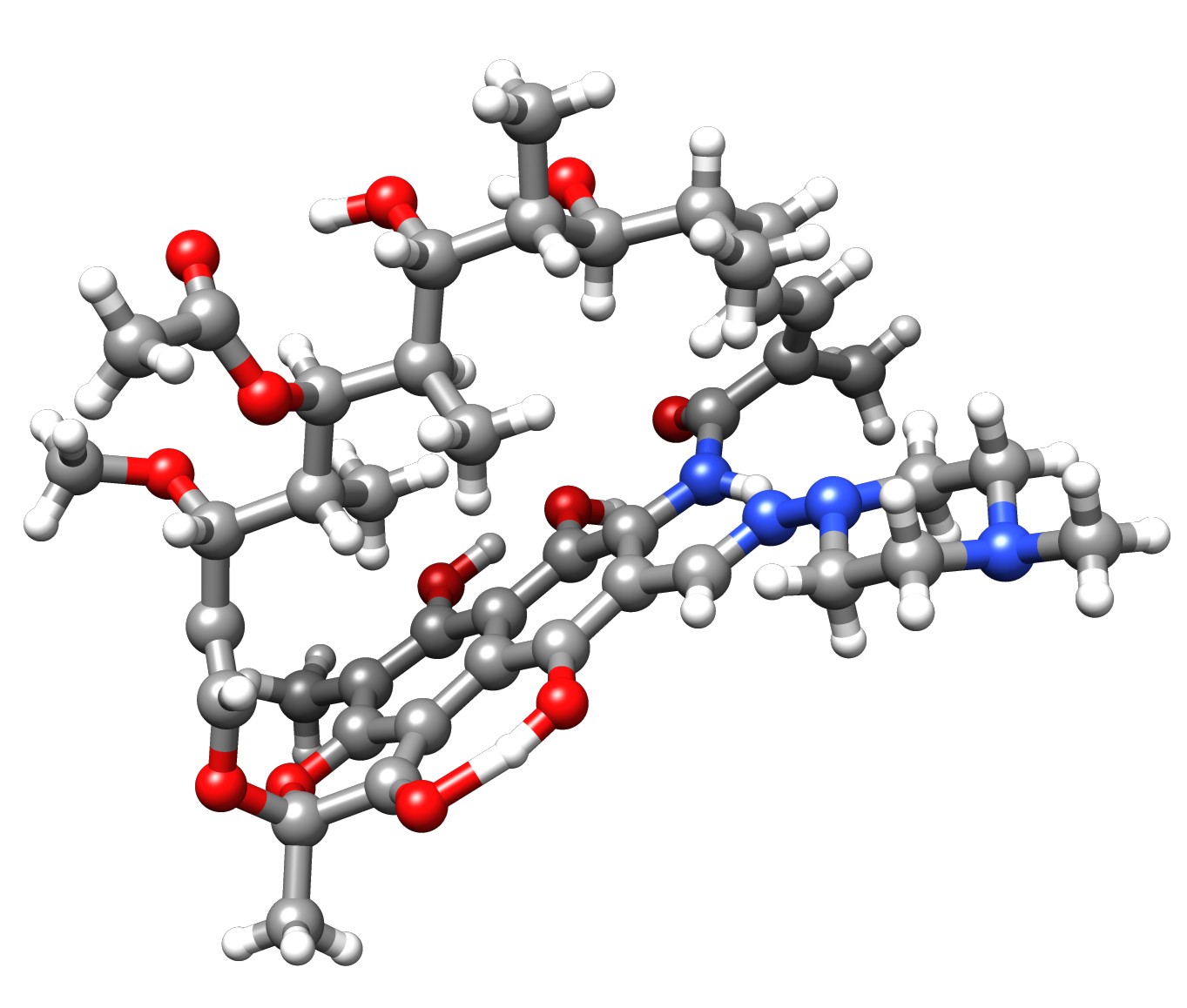
Figure 1: Rifampicin

Table 1: The lowest FC-CC2/aug-cc-pVDZ excitation energy $(\omega)$ of rifampicin. $n_{\mathrm{frozen}}$ is the number of frozen core orbitals.

$n_{\mathrm{AO}}$	$n_{\mathrm{MO}}$	$n_{\mathrm{frozen}}$	$\omega$
1879	1865	59	$2.5789\text{\,}\mathrm{eV}$

The CC2 method is known to yield excitation energies with an error of approximately $0.1\text{\,}\mathrm{eV}$ for states with single excitation character.(Christiansen et al., 1996; Kánnár and Szalay, 2014; Kánnár, Tajti, and Szalay, 2016) The iterative cost of CC2 scales as $\mathcal{O}(n_{\mathrm{MO}}^{5})$ and it may be implemented with an $\mathcal{O}(n_{\mathrm{MO}}^{2})$ memory requirement. In Table 1, we report the lowest FC-CC2/aug-cc-pVDZ excitation energy of the antibiotic rifampicin(rif, 2020) (chemical formula C₄₃H₅₈N₄O₁₂, see Figure 1). The calculated excitation energy is $2.58\text{\,}\mathrm{eV}$, which is consistent with the orange color of the compound and the experimental value of $2.61\text{\,}\mathrm{eV}$.(Benetton et al., 1998) The ground state was converged to a residual threshold of $10^{-6}$, and the excited state was converged to residual and energy thresholds of $10^{-3}$ and $10^{-6}$, respectively. We used a Cholesky decomposition threshold of $10^{-2}$, which is sufficient to ensure accuracy of excitation energies in CC2 and CCSD (see Table 4). The calculation was performed on two Intel Xeon Gold 6138 processors, using 40 threads and ${360}$ GB shared memory. The average iteration time for the ground state equations was $73\text{\,}\mathrm{min}$, and the average iteration time for the excited state equations was $9\text{\,}\mathrm{h}$.

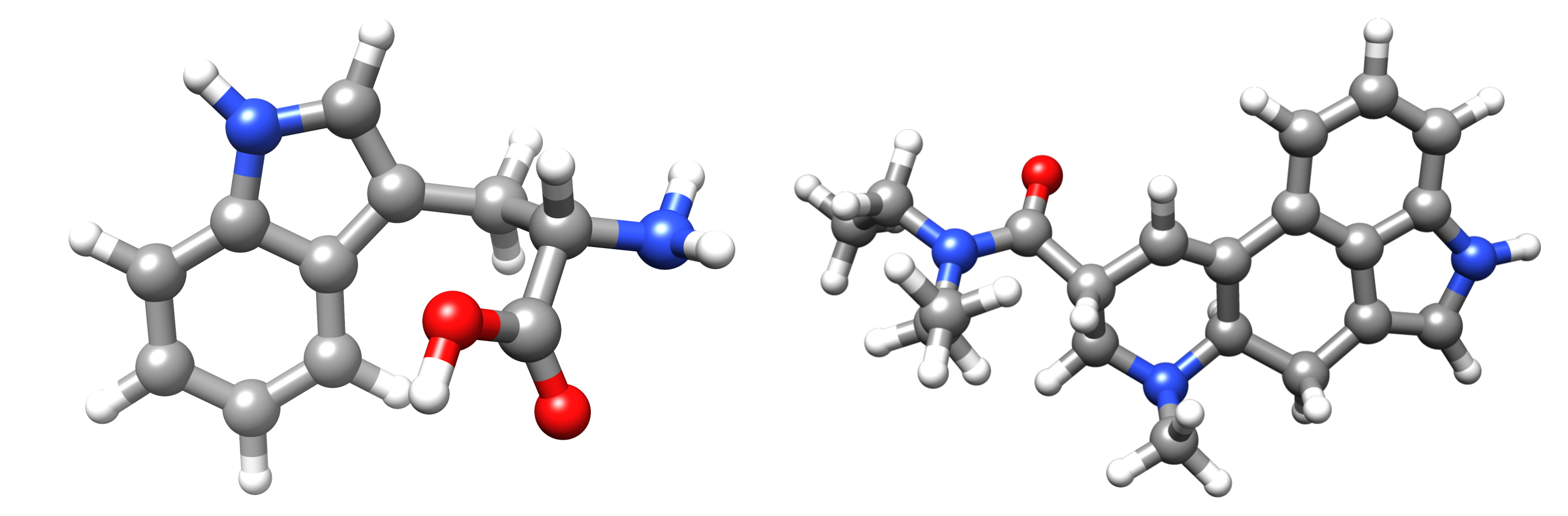
Figure 2: Tryptophan (left) and LSD (right)

Table 2: CCSD/aug-cc-pVDZ excitation energies $(\omega)$ and oscillator strengths $(f_{\omega})$ for tryptophan.

	$\omega~{}[$\mathrm{eV}$]$	$f_{\omega}$
$S_{1}$	4.806	0.032
$S_{2}$	4.821	0.001
$S_{3}$	4.972	0.088
$S_{4}$	5.364	0.001

Table 3: Total calculation times for CCSD/aug-cc-pVDZ ground state ($t_{\mathrm{gs}}$), excitation energy ($t_{\omega}$), and oscillator strength calculations ($t_{f_{\omega}}$) for tryptophan. $n_{\mathrm{calls}}^{\mathrm{gs}}$ is the number of calculations of the residual vector for the ground state. $n_{\mathrm{calls}}^{\mathrm{R}}$ and $n_{\mathrm{calls}}^{\mathrm{L}}$ are the number of calls to the Jacobian and Jacobian transpose transformations, respectively. The calculations were performed on an Intel Xeon E5-2699 v4 using 44 threads and 1.5 TB shared memory.

	$t_{\mathrm{gs}}~{}[$\mathrm{min}$]$	$t_{\omega}~{}[$\mathrm{h}$]$	$t_{f_{\omega}}~{}[$\mathrm{h}$]$	$n_{\mathrm{calls}}^{\mathrm{gs}}$	$n_{\mathrm{calls}}^{\mathrm{R}}$	$n_{\mathrm{calls}}^{\mathrm{L}}$
Dalton 2018	1409	84	–	18	88	–
$e^{T}$ 1.0	201	24	53	16	79	81
QChem 5.0	196	15	20	18	90	27

Table 4: The FC-CCSD/aug-cc-pVDZ correlation energy $(E_{\text{corr}})$ and lowest excitation energy $(\omega)$ of LSD. A set of decomposition thresholds $(\tau)$ for the Cholesky decomposition of the electron repulsion integral matrix were used. Both the ground and excited state equations are converged to within a residual threshold of $10^{-6}$. Deviations in the correlation and excitation energies ($\Delta E_{\text{corr}}$ and $\Delta\omega$), are relative to $\tau=10^{-8}$

$\tau$	$E_{\text{corr}}~{}[$\mathrm{\text{ $E_{\textup{ h }}$ }}$]$	$\Delta E_{\text{corr}}~{}[$\mathrm{\text{ $E_{\textup{ h }}$ }}$]$	$\omega~{}[$\mathrm{\text{ $E_{\textup{ h }}$ }}$]$	$\Delta\omega~{}[$\mathrm{\text{ $E_{\textup{ h }}$ }}$]$
$10^{-2}$	-3.6496733	$2.3\cdot 10^{-2}$	0.1657343	$7.1\cdot 10^{-4}$
$10^{-3}$	-3.6720218	$2.3\cdot 10^{-4}$	0.1650370	$7.7\cdot 10^{-6}$
$10^{-4}$	-3.6723421	$-9.2\cdot 10^{-5}$	0.1650279	$-1.4\cdot 10^{-6}$
$10^{-6}$	-3.6722542	$-3.6\cdot 10^{-6}$	0.1650294	$1.1\cdot 10^{-7}$
$10^{-8}$	-3.6722506	–	0.1650293	–

At the CCSD level of theory, we report calculations for the amino acid tryptophan(try, 2020) (chemical formula C₁₁H₁₂N₂O₂) and excitation energies for the psychoactive agent lysergic acid diethylamide (LSD)(lsd, 2020) (chemical formula C₂₀H₂₅N₃O₁). Tryptophan and LSD are depicted in Figure 2.

For tryptophan, we have determined the four lowest excitation energies and the corresponding oscillator strengths at the CCSD/aug-cc-pVDZ level of theory ($n_{\mathrm{MO}}=453$). Energies and oscillator strengths are reported in Table 2. Timings for $e^{T}$ 1.0, Dalton 2018, and QChem 5.0 are given in Table 3. Thresholds in $e^{T}$ were set to target an energy convergence of $10^{-6}$: the residuals were converged to $10^{-6}$ for the ground state and $10^{-3}$ for the excited states (assuming quadratic errors for the energy). In QChem, thresholds for ground and excited states were set to $10^{-6}$. We report the total wall time for each calculation. The excited state timing includes the time to converge ground state and excited state equations. The oscillator strength timing also includes the time to solve the multiplier and the left excited state equations. $e^{T}$ and QChem are equally efficient for the CCSD ground state, while Dalton is considerably slower. For the CCSD excited state calculation, QChem reduced the wall time by a factor of 1.6 compared to $e^{T}$ and a factor of 5.6 compared to Dalton. For the oscillator strength calculations, QChem reduced the wall time by a factor of 2.7 compared to $e^{T}$. The superior performance of QChem for oscillator strengths is primarily due to an efficient starting guess for the left excitation vectors: only 27 linear transformations are needed to converge all four roots.

We have performed FC-CCSD/aug-cc-pVDZ calculations on LSD ($n_{\mathrm{MO}}=777$, $n_{\mathrm{frozen}}=24$). To demonstrate the effect of integral approximation through Cholesky decomposition, we consider a range of decomposition thresholds. The correlation energy and the lowest excitation energy are given in Table 4. Both ground and excited state residual thresholds are $10^{-6}$. With a decomposition threshold of $10^{-2}$, the error in the excitation energy ($\Delta\omega$) is less than $10^{-3}$\mathrm{\text{ $E_{\textup{ h }}$ }}$$, well within the expected accuracy of FC-CCSD.(Christiansen et al., 1996; Kánnár and Szalay, 2014; Kánnár, Tajti, and Szalay, 2016)

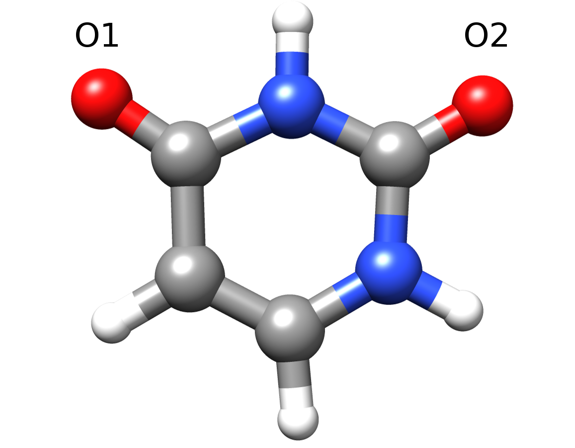
Figure 3: Uracil with labels on the oxygens

Table 5: Timing comparisons of $e^{T}$ 1.0 and Dalton 2018 for the lowest CC3/aug-cc-pVDZ excitation energy ($\omega$) of glycine. The calculations were performed on a node with two Intel Xeon Gold 6138 processors, using 40 threads and 320 GB shared memory.

$\omega$	$e^{T}$	Dalton (new)	Dalton (old)
$5.879\text{\,}\mathrm{eV}$	$33\text{\,}\mathrm{min}$	$73\text{\,}\mathrm{min}$	$1279\text{\,}\mathrm{min}$

Table 6: CC3 valence and core (oxygen edge) excitation energies $(\omega)$, and EOM oscillator strengths $(f_{\omega})$ for uracil. Valence excitations were calculated with the aug-cc-pVTZ basis on all atoms and the frozen core approximation. Core excitations were calculated using the CVS approximation with the aug-cc-pCVTZ basis on the oxygen atom being excited and the aug-cc-pVDZ basis on the remaining atoms.

	CCSD		CC3
	$\omega~{}[$\mathrm{eV}$]$	$f_{\omega}$	$\omega~{}[$\mathrm{eV}$]$	$f_{\omega}$
Valence	$5.08$	$2.24\cdot 10^{-8}$	$4.81$	$2.23\cdot 10^{-6}$
core O1	$536.04$	$3.35\cdot 10^{-2}$	$533.64$	$1.95\cdot 10^{-2}$
	$539.60$	$3.23\cdot 10^{-4}$	$535.66$	$2.24\cdot 10^{-4}$
core O2	$536.98$	$3.13\cdot 10^{-2}$	$534.64$	$1.32\cdot 10^{-2}$
	$539.44$	$1.47\cdot 10^{-4}$	$535.75$	$1.34\cdot 10^{-4}$

Table 7: Total wall times for CC3 on uracil. The valence calculation was performed on a node with two Intel Xeon Gold 6138 processors, using 40 threads and 320 GB shared memory. The CVS calculations were performed on a node with two Intel Xeon Gold 6138 processors, using 40 threads and 150 GB shared memory. n_o and n_v are the number of occupied and virtual orbitals, respectively.

Calculation	basis set	$t~{}[$\mathrm{h}$]$	no	nv
Valence excitation	aug-cc-pVTZ	147	21	431
CVS O1	aug-cc-pV(CT)Z	36	29	227
CVS O2	aug-cc-pV(CT)Z	38	29	227

Table 8: Average wall time per function call for both CC3 core excitation calculations on uracil. $n_{\mathrm{calls}}$ is the total number of routine calls in the two calculations.

Contributions	$t~{}[$\mathrm{min}$]$	$n_{\mathrm{calls}}$
Ground state amplitudes	14	28
Ground state multipliers	23	30
Right excited states	4	195
Left excited states	7	244

The CC3 model can be used to obtain highly accurate excitation energies. However, an iterative cost that scales as $\mathcal{O}(n_{\mathrm{v}}^{4}n_{\mathrm{o}}^{3})$ severely limits system size. To the best of our knowledge, $e^{T}$ includes the fastest available implementation of CC3. In Table 5, we compare $e^{T}$ timings to the new(Myhre and Koch, 2016) and efficient CC3 implementation, as well as the old(Hald et al., 2002) implementation, in Dalton 2018.(Aidas et al., 2014) The example system is glycine (chemical formula C₂H₅NO₂) with a geometry optimized at the CCSD(T)/aug-cc-pVDZ level using CFOUR.(Stanton et al., 2010) We have calculated ground and excited state energies and $e^{T}$ is twice as fast as the new implementation in Dalton.

We have calculated valence and core excitation energies and EOM oscillator strengths for the nucleobase uracil (chemical formula C₄H₄N₂O₂, see Figure 3). The geometry was optimized at the CCSD(T)/aug-cc-pVDZ level using CFOUR.(Stanton et al., 2010) One valence excitation energy was calculated at the FC-CCSD/aug-cc-pVTZ and FC-CC3/aug-cc-pVTZ levels of theory ($n_{\mathrm{MO}}=452$). Two core excited states were calculated for each of the oxygen atoms (O1 and O2, see Figure 3) at the CCSD and CC3 levels. The aug-cc-pCVTZ basis was used on the oxygen being excited and aug-cc-pVDZ on the remaining atoms ($n_{\mathrm{MO}}=256$). The results are given in Table 6. Total timings for the uracil calculations are presented in Table 7. In Table 8, we present averaged timings from the CVS calculations. They clearly demonstrate the reduced computational cost of the CVS implementation for CC3. The ground state calculation was about four times more expensive per iteration than the right excited state. Without the CVS approximation, the computational cost of the excited states scale as $4n_{\mathrm{v}}^{4}n_{\mathrm{o}}^{3}$ per iteration while the ground state scales as $2n_{\mathrm{v}}^{4}n_{\mathrm{o}}^{3}$. Using CVS, the excited state scaling is reduced to $4n_{\mathrm{v}}^{4}n_{\mathrm{o}}^{2}$.

III.2 Cholesky decomposition

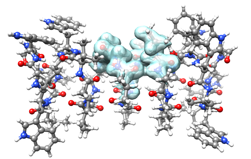
Figure 4: Gramicidin A. The active MLHF/cc-pVDZ density is shown.

Table 9: Cholesky decomposition wall times ($t$) for gramicidin. $\tau$ is the decomposition threshold and $n_{J}$ the number of Cholesky vectors. For reference, we include the time $(t^{\mathrm{HF}}_{\mathrm{it}})$ for one full Hartree-Fock iteration. All calculations were performed on an Intel Xeon E5-2699 v4 using 44 threads and 1.5 TB shared memory.

Basis	$n_{\mathrm{AO}}$	$\tau$	$n_{J}$	$t~{}[$\mathrm{min}$]$	$t^{\mathrm{HF}}_{\mathrm{it}}~{}[$\mathrm{min}$]$
cc-pVDZ	5188	$10^{-2}$	11574	3	35
		$10^{-3}$	16368	6
		$10^{-4}$	24652	12
		$10^{-8}$	75446	125
aug-cc-pVDZ	8740	$10^{-2}$	12813	8	1191
		$10^{-3}$	18587	27
		$10^{-4}$	29818	61
		$10^{-8}$	90656	645

We have determined the Cholesky basis for the transmembrane ion channel gramicidin A (chemical formula C₁₉₈H₂₇₆N₄₀O₃₄, see Figure 4). The geometry is taken from the supporting information of Ref. 81. Decomposition times are given in Table 9 for the cc-pVDZ and aug-cc-pVDZ basis sets and a range of decomposition thresholds. These are compared to the time of one HF iteration. Except when using cc-pVDZ with the tightest threshold, the decomposition time is small or negligible compared to one Fock matrix construction.

III.3 Hartree-Fock

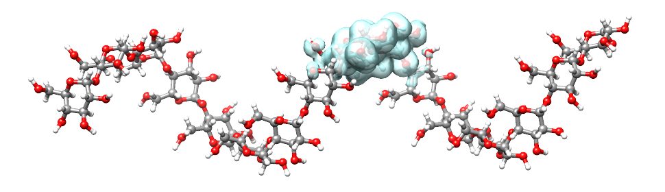
Figure 5: Amylose chain of 16 glucose units. The active MLHF/cc-pVDZ density is shown.

Table 10: Hartree-Fock/cc-pVDZ calculations on amylose and gramicidin. The total wall time is denoted by $t$ and $\tau_{\mathrm{SCF}}$ is the Hartree-Fock convergence threshold. We present timings for $e^{T}$ and QChem, along with the computed Hartree-Fock energies $(E)$ and absolute energy differences $(|\Delta E|)$ with respect to the calculation with the tightest threshold. Calculations were performed on two Intel Xeon E5-2699 v4 processors, using 44 threads and 1.5 TB shared memory.

	$e^{T}$					QChem
	$\tau_{\mathrm{SCF}}$	$E~{}[$\mathrm{\text{ $E_{\textup{ h }}$ }}$]$	$|\Delta E|~{}[$\mathrm{\text{ $E_{\textup{ h }}$ }}$]$	$t~{}[$\mathrm{min}$]$		$\tau_{\mathrm{SCF}}$	$E~{}[$\mathrm{\text{ $E_{\textup{ h }}$ }}$]$	$|\Delta E|~{}[$\mathrm{\text{ $E_{\textup{ h }}$ }}$]$	$t~{}[$\mathrm{min}$]$
amylose	$10^{-3}$	$-9792.08512990$	$4\cdot 10^{-5}$	21		$10^{-5}$	$-9792.08535039$	$2\cdot 10^{-4}$	9
	$10^{-4}$	$-9792.08517833$	$5\cdot 10^{-6}$	31		$10^{-6}$	$-9792.08518084$	$7\cdot 10^{-6}$	14
	$10^{-5}$	$-9792.08517442$	$7\cdot 10^{-7}$	42		$10^{-7}$	$-9792.08517119$	$2\cdot 10^{-6}$	19
	$10^{-6}$	$-9792.08517377$	$1\cdot 10^{-8}$	60		$10^{-8}$	$-9792.08517323$	$4\cdot 10^{-7}$	26
	$10^{-7}$	$-9792.08517376$	$<1\cdot 10^{-8}$	78		$10^{-9}$	$-9792.08517361$	$3\cdot 10^{-8}$	33
	$10^{-10}$	$-9792.08517376$	–	153		$10^{-10}$	$-9792.08517358$	–	46
gramicidin	$10^{-4}$	$-12383.45883254$	$4\cdot 10^{-6}$	130		$10^{-6}$	$-12383.45882513$	$1\cdot 10^{-5}$	50
	$10^{-5}$	$-12383.45883634$	$7\cdot 10^{-8}$	198		$10^{-7}$	$-12383.45882710$	$1\cdot 10^{-5}$	77
	$10^{-6}$	$-12383.45883627$	–	280		$10^{-8}$	$-12383.45883677$	–	111

Systems with several hundred atoms are easily modelled in $e^{T}$ using Hartree-Fock. In Table 10, we present wall times for calculations on gramicidin A (see Figure 4) and an amylose chain with 16 glucose units (chemical formula C₉₆H₁₆₂O₈₁, see Figure 5). The amylose geometry is taken from Sæther et al.(Sæther et al., 2017) We compare results and timings from $e^{T}$ 1.0 and QChem 5.0.(Shao et al., 2015) This comparison is complicated because the accuracy depends on several thresholds apart from the gradient and energy thresholds, e.g., screening thresholds and integral accuracy. We therefore list energies and absolute energy differences along with the timings in Table 10. QChem 5.0 outperforms $e^{T}$ by about factor of two. The energies converge to slightly different results in the two programs. In the case of amylose, we find a $2\cdot{10^{-7}}~{}$\mathrm{\text{ $E_{\textup{ h }}$ }}$$ energy difference using the tightest thresholds ($\tau_{\mathrm{SCF}}=10^{-10}$). We are able to reproduce the $e^{T}$ results using tight thresholds in LSDalton 2018.(Aidas et al., 2014)

III.4 Multilevel and multiscale methods

Table 11: The two lowest excitation energies ($\omega_{1}$ and $\omega_{2}$) of $\text{SO}_{2}$ with 21 water molecules, calculated with full, and reduced space FC-CC2 and FC-MLCC2, using HF and MLHF reference wave functions. Deviation from full FC-CC2 ($\Delta\omega_{i}=\omega_{i}-\omega_{i}^{\text{FC-CC2}}$) are given. We also list the number of occupied ($n_{\mathrm{o}}$) and virtual ($n_{\mathrm{v}}$) orbitals treated at the different levels of theory. There are a total of $121$ occupied orbitals and $813$ virtual orbitals in the system.

Calculation	HF		CCS		CC2		$\omega_{1}~{}[$\mathrm{eV}$]$	$\Delta\omega_{1}~{}[$\mathrm{eV}$]$	$\omega_{2}~{}[$\mathrm{eV}$]$	$\Delta\omega_{1}~{}[$\mathrm{eV}$]$
	$n_{\mathrm{o}}$	$n_{\mathrm{v}}$	$n_{\mathrm{o}}$	$n_{\mathrm{v}}$	$n_{\mathrm{o}}$	$n_{\mathrm{v}}$
FC-CC2	121	813	–	–	93	813	3.11	–	3.39	–
FC-CC2-in-HF	121	813	–	–	40	266	3.14	0.03	3.43	0.04
FC-CC2-in-MLHF	75	426	–	–	40	266	3.16	0.05	3.44	0.05
FC-MLCC2	121	813	93	813	14	67	3.18	0.07	3.45	0.06
FC-MLCC2-in-HF	121	813	40	266	14	66	3.18	0.07	3.45	0.06
FC-MLCC2-in-MLHF	75	426	40	266	15	66	3.20	0.09	3.47	0.08

To demonstrate the efficacy of multilevel methods for excitation energies, we consider a system of sulfur dioxide with 21 water molecules, (see Figure 6). In Table 11, we present different flavours of multilevel calculations to approximate the two lowest FC-CC2 excitation energies for this system. Three sets of active atoms are defined. The first set contains the sulfur dioxide and nine water molecules; these atoms determine the active orbitals of the MLHF calculation. The second set contains the sulfur dioxide and five water molecules; these atoms determine the reduced space coupled cluster calculations. The third set contains only sulfur dioxide and determines the CC2 active space in the MLCC2 calculations. The reduced space FC-CC2 calculations are denoted FC-CC2-in-HF and FC-CC2-in-MLHF and similarly for the reduced space FC-MLCC2 calculations. Orbital spaces are partitioned using Cholesky occupied orbitals and PAOs for the virtual orbitals. In all calculations, the deviation with respect to full FC-CC2 is within the expected error of CC2, which is about $0.1\text{\,}\mathrm{eV}$.Kánnár and Szalay (2014); Kánnár, Tajti, and Szalay (2016)

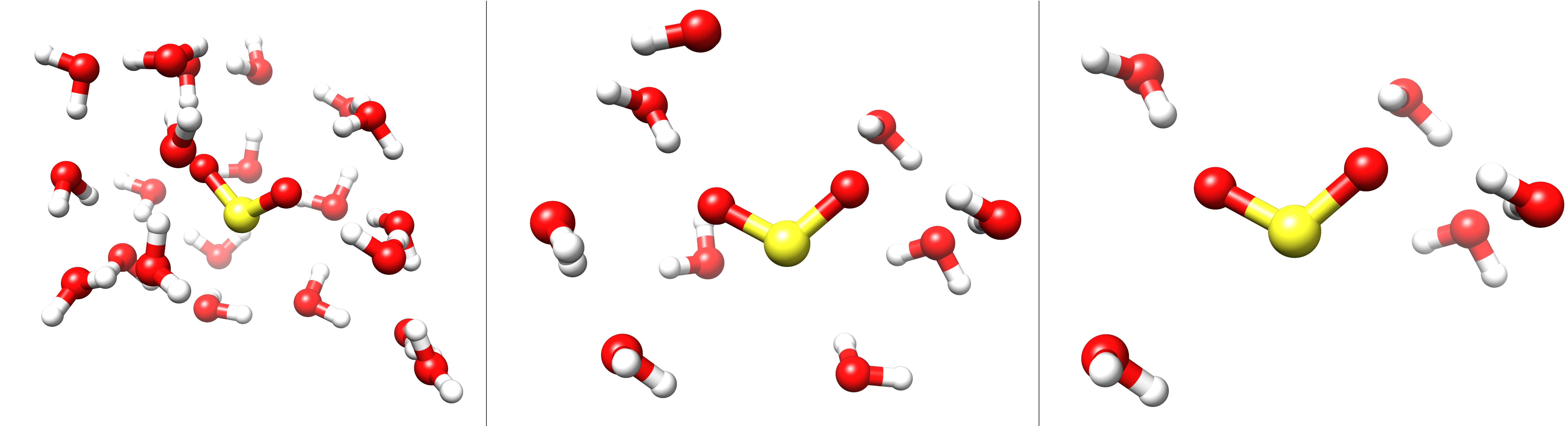
Figure 6: $\text{SO}_{2}$ and water. On the left, $\text{SO}_{2}$ and 21 water molecules. In the middle, $\text{SO}_{2}$ and nine water molecules; these are the HF active atoms in the MLHF calculations. On the right, $\text{SO}_{2}$ and five water molecules; these are the CC active atoms. In the MLCC2 calculations only $\text{SO}_{2}$ is treated at the CC2 level of theory.

Table 12: Multilevel Hartree-Fock wall times for amylose and gramicidin. $t_{\mathrm{it}}$ is the wall time to construct the Fock matrix. For the calculations with (aug)-cc-pVDZ, aug-cc-pVDZ is used on the active atoms and cc-pVDZ for the rest. The total number of AOs and the active MOs are labelled $n_{\mathrm{AO}}$ and $n_{\mathrm{MO}}^{\mathrm{active}}$. Thresholds for Coulomb and exchange are set to $10^{-12}$ and $10^{-10}$, respectively, and the integral cutoff to $10^{-12}$. Calculations were performed on two Intel Xeon E5-2699 v4 processors, using 44 threads and 1.5 TB shared memory.

		HF		MLHF
	Basis	$n_{\mathrm{AO}}$	$t_{\mathrm{it}}~{}[$\mathrm{min}$]$	$n_{\mathrm{MO}}^{\mathrm{active}}$	$t_{\mathrm{it}}~{}[$\mathrm{min}$]$
amylose	cc-pVDZ	3288	8	335	1
	(aug)-cc-pVDZ	3480	11	552	4
gramicidin	cc-pVDZ	5188	35	546	11
	(aug)-cc-pVDZ	5506	69	942	50

In order to assess the performance of the MLHF implementation, we compare full HF and MLHF for gramicidin A and amylose. Active electron densities from the MLHF calculations are shown in Figures 4 and 5. The plots were generated using UCSF Chimera.(Pettersen et al., 2004) Cholesky orbitals were used to partition the occupied space and PAOs were used for the virtual space. We present timings in Table 12. For amylose, the iteration times are reduced significantly with MLHF: by a factor of eight when cc-pVDZ is used on all atoms and a factor of three when aug-cc-pVDZ is used on the active atoms. In contrast, only a factor of three was reported by Sæther et al.(Sæther et al., 2017) in the cc-pVDZ case. The iteration time is also reduced by a factor of eight for amylose/cc-pVDZ ($t_{\mathrm{iteration}}=1$ m, $n_{\mathrm{MO}}^{\mathrm{active}}=318$) when using Cholesky virtuals (as in Ref.23) instead of PAOs. The savings for amylose reflect the small active region as well as the linear structure of the chain. Savings are less significant for the gramicidin system, where the MLHF iteration time is a third of the HF iteration time for cc-pVDZ, but only about two thirds when the active atoms are described using aug-cc-pVDZ. The smaller savings reflect the relatively large active region and the more compact shape of the gramicidin system.

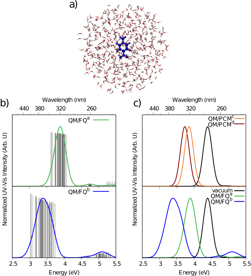
Figure 7: a) Schematic representation of a random snapshot of PNA in aqueous solution. b) and c) UV/Vis spectra of PNA calculated at the CC2/aug-cc-pVDZ level of theory with an aqueous solution described at the PCM or FQ level of theory. b) QM/FQ raw data (sticks) together with their Gaussian convolution (FWHM = 0.3 eV). c) QM/PCM (top) and QM/FQ (bottom) spectra in aqueous solution. A gas phase CC2/aug-cc-pVDZ reference spectrum is also reported (black). For QM/FQ${}^{\text{a}}$, the FQ parametrization is from Ref. 83 and for QM/FQ${}^{\text{b}}$, the parametrization is from Ref. 84. In QM/FQ${}^{\text{c}}$, the PCM cavity is constructed using the UFF radii,Rappe et al. (1992) and in QM/FQ${}^{\text{d}}$ it is constructed using the Bondi radii.Bondi (1964)

Table 13: The first vertical excitation energy of PNA in vacuum ($\omega_{\mathrm{v}}$) and in aqueous solution ($\omega_{\mathrm{s}}$), as well as water-to-vacuum solvatochromatic shifts $(\Delta\omega)$. PNA is treated at the CC2/aug-cc-pVDZ level of theory, and the solution is described with PCM or FQ. 68% confidence intervals for excitation energies are also reported for QM/FQ, calculated as $\sigma/\sqrt{N}$, where $\sigma$ is the standard deviation and $N$ is the number of the snapshots used to obtain the average property. Experimental data are taken from Ref. 87.

	$\omega_{\mathrm{v}}$ $[$\mathrm{eV}$]$	$\omega_{\mathrm{s}}$ $[$\mathrm{eV}$]$	$\Delta\omega$ $[$\mathrm{eV}$]$
CC2	4.38	–	–
CC2/FQa	–	3.88$\pm$0.01	0.50$\pm$0.01
CC2/FQb	–	3.38$\pm$0.01	1.00$\pm$0.01
CC2/PCMc	–	3.86	0.52
CC2/PCMd	–	3.76	0.62
Experimente	4.25	3.26	0.99

• FQ parametrization taken from Ref. 83

• FQ parametrization taken from Ref. 84

• PCM cavity constructed by exploiting UFF radii.Rappe et al. (1992)

• PCM cavity constructed by exploiting Bondi radii.Bondi (1964)

• Ref. 87

For systems in solution, electronic spectra can be calculated using QM/MM or QM/PCM. Paranitroaniline (PNA) has an experimental vacuum-to-water solvatochromism of about $1\text{\,}\mathrm{eV}$.Kovalenko et al. (2000) For QM/PCM, we use two different atomic radii, UFF(Rappe et al., 1992) (QM/PCM${}^{\text{c}}$) and Bondi(Bondi, 1964) (QM/PCM${}^{\text{d}}$), and the dielectric permittivity of water was set to $\varepsilon=78.39$. For QM/MM, 64 snapshots were extracted from a classical molecular dynamics simulation.(Giovannini et al., 2019b) See Figure 7a for an example structure. The UV/Vis spectra were then computed by treating PNA at the CC2/aug-cc-pVDZ level and modelling the water using an FQ force field. Here, we present results using two different FQ parametrizations: QM/FQ${}^{\text{a}}$ from Ref. 83 and QM/FQ${}^{\text{b}}$ from Ref. 84. See the supplemental material for additional computational details.

The spectra calculated using QM/FQ are presented in Figure 7b. Results for individual snapshots are presented as sticks together with their Gaussian convolution. As can be seen from Figure 7, QM/FQ^b results in a greater spread in the excitation energies. This is probably due to the larger molecular dipole moments of the water molecules in this parametrization.Giovannini et al. (2019b, c)

In Figure 7c, convoluted spectra calculated using QM/PCM${}^{\text{c}}$ and QM/PCM${}^{\text{d}}$ (top), and QM/FQ${}^{\text{a}}$ and QM/FQ${}^{\text{b}}$ (bottom), are presented with their vacuum counterparts. The excitation energies are also given in Table 13 together with experimental data from Ref. 87. For QM/FQ, we also report 68% confidence intervals for the calculated excitation energies. QM/FQ^b reproduces the experimental solvatochromism, while the other approaches give errors of 40-50%.

III.5 Modelling spectroscopies

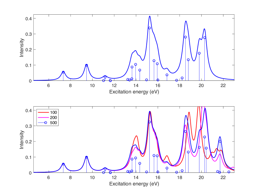
Figure 8: Water CCSD/aug-cc-pCVDZ UV/Vis absorption spectrum. Lorentzian broadening ($0.02\text{\,}\mathrm{\text{ $E_{\textup{ h }}$ }}$ FWHM) has been applied to the stick spectra. The top plot shows the spectrum obtained using Davidson. The spectrum in the bottom plot is from Lanczos calculations with chain lengths $100$ (red), $200$ (magenta), and $500$ (blue).

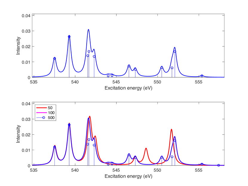
Figure 9: Water CCSD/CVS/aug-cc-pCVDZ X-ray absorption spectrum. Lorentzian broadening ($0.02\text{\,}\mathrm{\text{ $E_{\textup{ h }}$ }}$ FWHM) has been applied to the stick spectra. The top plot shows the spectrum obtained using Davidson. The spectrum in the bottom plot is from Lanczos calculations with chain lengths $50$ (red), $100$ (magenta), and $500$ (blue).

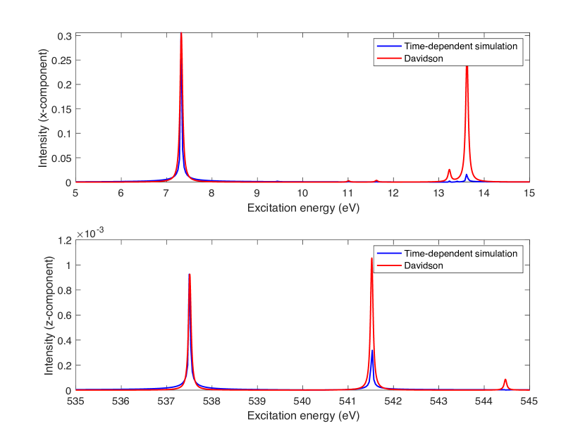
Figure 10: Water UV and X-ray CCSD absorption spectra obtained using Davidson (CVS/aug-cc-pCVDZ for X-ray, aug-cc-pVDZ for UV) and real-time propagation (aug-cc-pCVDZ for X-ray, aug-cc-pVDZ for UV). The top and bottom plots show simulated UV and X-ray spectra, respectively. The Davidson spectra were produced by applying Lorentzian broadening to the stick spectra ($0.0025\text{\,}\mathrm{\text{ $E_{\textup{ h }}$ }}$ FWHM). Intensities from the time-dependent simulation have been scaled so that the intensity of the first peak matches the EOM oscillator strength.

Spectroscopic properties can also be modelled with the Lanczos method or with real-time propagation of the coupled cluster wave function. In Figure 8, we show CCSD/aug-cc-pCVDZ UV/Vis absorption spectra of H₂O,(Olsen et al., 1996) calculated using the Davidson (top) and asymmetric Lanczos (bottom) algorithms. Note that we have artificially extended the spectra beyond the ionization potential ($12.3\text{\,}\mathrm{eV}$ IP-CCSD/aug-cc-pCVDZ) to illustrate convergence behavior. With the Lanczos algorithm, the low energy part of the spectrum converges with a smaller reduced space than the high energy part.(Coriani et al., 2012)

We have also generated oxygen edge X-ray absorption spectra using the Davidson and Lanczos algorithms with CVS projection; see Figure 9. We see the same overall behavior as in Figure 8.

Absorption spectra can also be obtained from real-time propagation of the coupled cluster wavefunction. See Figure 10 for UV/Vis and oxygen edge X-ray absorption spectra. See the supplemental material for computational details. The first peak in both plots has been scaled to match the intensity obtained using Davidson. The position of the peaks are the same with both approaches, but the intensities differ because we specified pulses with frequency distributions centered on the first excitation energy.

IV Concluding remarks

$e^{T}$ 1.0  is an optimized open source electronic structure program. Several features are worth emphasizing. To the best of our knowledge, our CC3 implementation is the fastest for calculating ground and excited state energies and EOM oscillator strengths. The low memory CC2 code has memory and disk requirements of order $\mathcal{O}(n_{\mathrm{MO}}^{2})$ and $\mathcal{O}(n_{\mathrm{MO}}^{3})$, respectively, allowing us to treat systems with thousands of basis functions. At the core of our program is the Cholesky decomposition of the electron repulsion integral matrix; our implementation is faster and less storage intensive than that of any other program. Exciting new developments are also part of $e^{T}$. It features the only spin adapted closed shell implementation of time-dependent coupled cluster theory. Furthermore, the MLHF and MLCC2 methods extend the treatable system size without sacrificing accuracy for intensive properties such as excitation energies.

The $e^{T}$ source code is written in modern object oriented Fortran, making it easy to expand and contribute to the program. It is freely available on GitLab(Folkestad et al., 2020) and the manual can be found at www.etprogram.org. We will continue to expand the capabilities of $e^{T}$, focusing on molecular properties and multilevel methods. We believe the program will be useful for the quantum chemistry community, both as a development platform and for production calculations.

V Acknowledgements

We thank Sander Roet for useful discussions regarding Python and Git functionality. We thank Franco Egidi, Laura Grazioli, Gioia Marrazzini, Rosario Roberto Riso, and Anna Kristina Schnack-Petersen, who attended the $e^{T}$ workshop in Pisa, October/November 2019. We also thank Edward Valeev for assistance with Libint and Roberto Di Remigio for help with a patch of PCMSolver. We acknowledge computing resources through UNINETT Sigma2 - the National Infrastructure for High Performance Computing and Data Storage in Norway, through project number NN2962k and NN9409k, and the SMART@SNS Laboratory. We acknowledge funding from the Marie Skłodowska-Curie European Training Network “COSINE - COmputational Spectroscopy In Natural sciences and Engineering”, Grant Agreement No. 765739, the Research Council of Norway through FRINATEK projects 263110 and 275506. S.C. acknowledges support from the Independent Research Fund Denmark – DFF-RP2 grant no. 7014-00258B

References

- Helgaker, Jørgensen, and Olsen (2014) T. Helgaker, P. Jørgensen, and J. Olsen, Molecular electronic-structure theory (John Wiley & Sons, 2014).
- Stanton et al. (2010) J. Stanton, J. Gauss, M. Harding, P. Szalay, A. Auer, R. Bartlett, U. Benedikt, C. Berger, D. Bernholdt, Y. Bomble, et al., “CFOUR, coupled-cluster techniques for computational chemistry, a quantum-chemical program package,” Current version available at http://www. cfour. de (2010).
- Aidas et al. (2014) K. Aidas, C. Angeli, K. L. Bak, V. Bakken, R. Bast, L. Boman, O. Christiansen, R. Cimiraglia, S. Coriani, P. Dahle, E. K. Dalskov, U. Ekström, T. Enevoldsen, J. J. Eriksen, P. Ettenhuber, B. Fernández, L. Ferrighi, H. Fliegl, L. Frediani, K. Hald, A. Halkier, C. Hättig, H. Heiberg, T. Helgaker, A. C. Hennum, H. Hettema, E. Hjertenæs, S. Høst, I.-M. Høyvik, M. F. Iozzi, B. Jansík, H. J. A. Jensen, D. Jonsson, P. Jørgensen, J. Kauczor, S. Kirpekar, T. Kjærgaard, W. Klopper, S. Knecht, R. Kobayashi, H. Koch, J. Kongsted, A. Krapp, K. Kristensen, A. Ligabue, O. B. Lutnæs, J. I. Melo, K. V. Mikkelsen, R. H. Myhre, C. Neiss, C. B. Nielsen, P. Norman, J. Olsen, J. M. H. Olsen, A. Osted, M. J. Packer, F. Pawlowski, T. B. Pedersen, P. F. Provasi, S. Reine, Z. Rinkevicius, T. A. Ruden, K. Ruud, V. V. Rybkin, P. Sałek, C. C. M. Samson, A. S. de Merás, T. Saue, S. P. A. Sauer, B. Schimmelpfennig, K. Sneskov, A. H. Steindal, K. O. Sylvester-Hvid, P. R. Taylor, A. M. Teale, E. I. Tellgren, D. P. Tew, A. J. Thorvaldsen, L. Thøgersen, O. Vahtras, M. A. Watson, D. J. D. Wilson, M. Ziolkowski, and H. Ågren, “The Dalton quantum chemistry program system,” WIREs Comput. Mol. Sci. 4, 269–284 (2014), https://onlinelibrary.wiley.com/doi/pdf/10.1002/wcms.1172 .
- Gordon and Schmidt (2005) M. S. Gordon and M. W. Schmidt, “Chapter 41 - advances in electronic structure theory: GAMESS a decade later,” in Theory and Applications of Computational Chemistry, edited by C. E. Dykstra, G. Frenking, K. S. Kim, and G. E. Scuseria (Elsevier, Amsterdam, 2005) pp. 1167 – 1189.
- Aquilante et al. (2016) F. Aquilante, J. Autschbach, R. K. Carlson, L. F. Chibotaru, M. G. Delcey, L. De Vico, I. Fdez. Galván, N. Ferré, L. M. Frutos, L. Gagliardi, M. Garavelli, A. Giussani, C. E. Hoyer, G. Li Manni, H. Lischka, D. Ma, P. Å. Malmqvist, T. Müller, A. Nenov, M. Olivucci, T. B. Pedersen, D. Peng, F. Plasser, B. Pritchard, M. Reiher, I. Rivalta, I. Schapiro, J. Segarra-Martí, M. Stenrup, D. G. Truhlar, L. Ungur, A. Valentini, S. Vancoillie, V. Veryazov, V. P. Vysotskiy, O. Weingart, F. Zapata, and R. Lindh, “Molcas 8: New capabilities for multiconfigurational quantum chemical calculations across the periodic table,” J. Comput. Chem. 37, 506–541 (2016), https://onlinelibrary.wiley.com/doi/pdf/10.1002/jcc.24221 .
- Werner et al. (2012) H.-J. Werner, P. J. Knowles, G. Knizia, F. R. Manby, and M. Schütz, “Molpro: a general-purpose quantum chemistry program package,” WIREs Comput. Mol. Sci. 2, 242–253 (2012).
- Valiev et al. (2010) M. Valiev, E. Bylaska, N. Govind, K. Kowalski, T. Straatsma, H. V. Dam, D. Wang, J. Nieplocha, E. Apra, T. Windus, and W. de Jong, “NWChem: A comprehensive and scalable open-source solution for large scale molecular simulations,” Comput. Phys. Commun. 181, 1477 – 1489 (2010).
- Neese (2012) F. Neese, “The orca program system,” WIREs Comput. Mol. Sci. 2, 73–78 (2012).
- Parrish et al. (2017) R. M. Parrish, L. A. Burns, D. G. A. Smith, A. C. Simmonett, A. E. DePrince, E. G. Hohenstein, U. Bozkaya, A. Y. Sokolov, R. Di Remigio, R. M. Richard, J. F. Gonthier, A. M. James, H. R. McAlexander, A. Kumar, M. Saitow, X. Wang, B. P. Pritchard, P. Verma, H. F. Schaefer, K. Patkowski, R. A. King, E. F. Valeev, F. A. Evangelista, J. M. Turney, T. D. Crawford, and C. D. Sherrill, “Psi4 1.1: An open-source electronic structure program emphasizing automation, advanced libraries, and interoperability,” J. Chem. Theor. Comput. 13, 3185–3197 (2017), https://doi.org/10.1021/acs.jctc.7b00174 .
- Shao et al. (2015) Y. Shao, Z. Gan, E. Epifanovsky, A. T. Gilbert, M. Wormit, J. Kussmann, A. W. Lange, A. Behn, J. Deng, X. Feng, D. Ghosh, M. Goldey, P. R. Horn, L. D. Jacobson, I. Kaliman, R. Z. Khaliullin, T. Kuś, A. Landau, J. Liu, E. I. Proynov, Y. M. Rhee, R. M. Richard, M. A. Rohrdanz, R. P. Steele, E. J. Sundstrom, H. L. W. III, P. M. Zimmerman, D. Zuev, B. Albrecht, E. Alguire, B. Austin, G. J. O. Beran, Y. A. Bernard, E. Berquist, K. Brandhorst, K. B. Bravaya, S. T. Brown, D. Casanova, C.-M. Chang, Y. Chen, S. H. Chien, K. D. Closser, D. L. Crittenden, M. Diedenhofen, R. A. D. Jr., H. Do, A. D. Dutoi, R. G. Edgar, S. Fatehi, L. Fusti-Molnar, A. Ghysels, A. Golubeva-Zadorozhnaya, J. Gomes, M. W. Hanson-Heine, P. H. Harbach, A. W. Hauser, E. G. Hohenstein, Z. C. Holden, T.-C. Jagau, H. Ji, B. Kaduk, K. Khistyaev, J. Kim, J. Kim, R. A. King, P. Klunzinger, D. Kosenkov, T. Kowalczyk, C. M. Krauter, K. U. Lao, A. D. Laurent, K. V. Lawler, S. V. Levchenko, C. Y. Lin, F. Liu, E. Livshits, R. C. Lochan, A. Luenser, P. Manohar, S. F. Manzer, S.-P. Mao, N. Mardirossian, A. V. Marenich, S. A. Maurer, N. J. Mayhall, E. Neuscamman, C. M. Oana, R. Olivares-Amaya, D. P. O’Neill, J. A. Parkhill, T. M. Perrine, R. Peverati, A. Prociuk, D. R. Rehn, E. Rosta, N. J. Russ, S. M. Sharada, S. Sharma, D. W. Small, A. Sodt, T. Stein, D. Stück, Y.-C. Su, A. J. Thom, T. Tsuchimochi, V. Vanovschi, L. Vogt, O. Vydrov, T. Wang, M. A. Watson, J. Wenzel, A. White, C. F. Williams, J. Yang, S. Yeganeh, S. R. Yost, Z.-Q. You, I. Y. Zhang, X. Zhang, Y. Zhao, B. R. Brooks, G. K. Chan, D. M. Chipman, C. J. Cramer, W. A. G. III, M. S. Gordon, W. J. Hehre, A. Klamt, H. F. S. III, M. W. Schmidt, C. D. Sherrill, D. G. Truhlar, A. Warshel, X. Xu, A. Aspuru-Guzik, R. Baer, A. T. Bell, N. A. Besley, J.-D. Chai, A. Dreuw, B. D. Dunietz, T. R. Furlani, S. R. Gwaltney, C.-P. Hsu, Y. Jung, J. Kong, D. S. Lambrecht, W. Liang, C. Ochsenfeld, V. A. Rassolov, L. V. Slipchenko, J. E. Subotnik, T. V. Voorhis, J. M. Herbert, A. I. Krylov, P. M. Gill, and M. Head-Gordon, “Advances in molecular quantum chemistry contained in the Q-Chem 4 program package,” Mol. Phys. 113, 184–215 (2015), https://doi.org/10.1080/00268976.2014.952696 .
- Furche et al. (2014) F. Furche, R. Ahlrichs, C. Hättig, W. Klopper, M. Sierka, and F. Weigend, “Turbomole,” WIREs Comput. Mol. Sci. 4, 91–100 (2014).
- Helgaker et al. (2012) T. Helgaker, S. Coriani, P. Jørgensen, K. Kristensen, J. Olsen, and K. Ruud, “Recent advances in wave function-based methods of molecular-property calculations,” Chem. Rev. 112, 543–631 (2012), https://doi.org/10.1021/cr2002239 .
- Koch et al. (1990) H. Koch, H. J. A. Jensen, P. Jørgensen, T. Helgaker, G. E. Scuseria, and H. F. Schaefer, “Coupled cluster energy derivatives. analytic hessian for the closed-shell coupled cluster singles and doubles wave function: Theory and applications,” J. Chem. Phys. 92, 4924–4940 (1990), https://doi.org/10.1063/1.457710 .
- Stanton (1993) J. F. Stanton, “Many-body methods for excited state potential energy surfaces. i. general theory of energy gradients for the equation-of-motion coupled-cluster method,” J. Chem. Phys. 99, 8840–8847 (1993), https://doi.org/10.1063/1.465552 .
- Stanton and Bartlett (1993) J. F. Stanton and R. J. Bartlett, “The equation of motion coupled-cluster method. a systematic biorthogonal approach to molecular excitation energies, transition probabilities, and excited state properties,” J. Chem. Phys. 98, 7029–7039 (1993), https://doi.org/10.1063/1.464746 .
- Krylov (2008) A. I. Krylov, “Equation-of-motion coupled-cluster methods for open-shell and electronically excited species: The hitchhiker’s guide to fock space,” Ann. Rev. Phys. Chem. 59, 433–462 (2008), https://doi.org/10.1146/annurev.physchem.59.032607.093602 .
- Beebe and Linderberg (1977) N. H. F. Beebe and J. Linderberg, “Simplifications in the generation and transformation of two-electron integrals in molecular calculations,” Int. J. Quantum Chem. 12, 683–705 (1977), https://onlinelibrary.wiley.com/doi/pdf/10.1002/qua.560120408 .
- Koch, Sánchez de Merás, and Pedersen (2003) H. Koch, A. Sánchez de Merás, and T. B. Pedersen, “Reduced scaling in electronic structure calculations using Cholesky decompositions,” J. Chem. Phys. 118, 9481–9484 (2003), https://doi.org/10.1063/1.1578621 .
- Coester and Kümmel (1960) F. Coester and H. Kümmel, “Short-range correlations in nuclear wave functions,” Nuclear Physics 17, 477 – 485 (1960).
- Folkestad, Kjønstad, and Koch (2019) S. D. Folkestad, E. F. Kjønstad, and H. Koch, “An efficient algorithm for Cholesky decomposition of electron repulsion integrals,” J. Chem. Phys. 150, 194112 (2019), https://doi.org/10.1063/1.5083802 .
- Koch et al. (1997) H. Koch, O. Christiansen, P. Jørgensen, A. M. Sanchez de Merás, and T. Helgaker, “The CC3 model: An iterative coupled cluster approach including connected triples,” J. Chem. Phys. 106, 1808–1818 (1997), https://doi.org/10.1063/1.473322 .
- Myhre and Koch (2016) R. H. Myhre and H. Koch, “The multilevel CC3 coupled cluster model,” J. Chem. Phys. 145, 44111 (2016).
- Sæther et al. (2017) S. Sæther, T. Kjærgaard, H. Koch, and I.-M. Høyvik, “Density-based multilevel hartree–fock model,” J. Chem. Theor. Comput. 13, 5282–5290 (2017).
- Myhre, Sánchez de Merás, and Koch (2014) R. H. Myhre, A. M. J. Sánchez de Merás, and H. Koch, “Multi-level coupled cluster theory,” J. Chem. Phys. 141, 224105 (2014).
- Folkestad and Koch (2019) S. D. Folkestad and H. Koch, “The multilevel CC2 and CCSD methods with correlated natural transition orbitals,” J. Chem. Theor. Comput. (2019).
- Warshel and Karplus (1972) A. Warshel and M. Karplus, “Calculation of ground and excited state potential surfaces of conjugated molecules. i. formulation and parametrization,” J. Am. Chem. Soc. 94, 5612–5625 (1972).
- Levitt and Warshel (1975) M. Levitt and A. Warshel, “Computer simulation of protein folding,” Nature 253, 694 (1975).
- Tomasi, Mennucci, and Cammi (2005) J. Tomasi, B. Mennucci, and R. Cammi, “Quantum mechanical continuum solvation models,” Chem. Rev. 105, 2999–3094 (2005).
- Mennucci (2012) B. Mennucci, “Polarizable continuum model,” WIREs Comput. Mol. Sci. 2, 386–404 (2012).
- Valeev (2017) E. Valeev, “Libint: A library for the evaluation of molecular integrals of many-body operators over gaussian functions,” (2017).
- Di Remigio et al. (2019a) R. Di Remigio, A. H. Steindal, K. Mozgawa, V. Weijo, H. Cao, and L. Frediani, “Pcmsolver: An open-source library for solvation modeling,” Int. J. Quantum Chem. 119, e25685 (2019a).
- Bast (2018) R. Bast, “Runtest,” (2018), https://doi.org/10.5281/zenodo.1434751.
- Bast, Di Remigio, and Juselius (2020) R. Bast, R. Di Remigio, and J. Juselius, “Autocmake,” (2020), https://doi.org/10.5281/zenodo.3634941.
- (34) Https://www.openmp.org/spec-html/5.0/openmp.html.
- Christiansen, Koch, and Jørgensen (1995) O. Christiansen, H. Koch, and P. Jørgensen, “The second-order approximate coupled cluster singles and doubles model CC2,” Chem. Phys. Lett. 243, 409 – 418 (1995).
- Purvis and Bartlett (1982) G. D. Purvis and R. J. Bartlett, “A full coupled-cluster singles and doubles model: The inclusion of disconnected triples,” J. Chem. Phys. 76, 1910–1918 (1982), https://doi.org/10.1063/1.443164 .
- Raghavachari et al. (1989) K. Raghavachari, G. W. Trucks, J. A. Pople, and M. Head-Gordon, “A fifth-order perturbation comparison of electron correlation theories,” Chem. Phys. Lett. 157, 479 – 483 (1989).
- Davidson (1975) E. R. Davidson, “The iterative calculation of a few of the lowest eigenvalues and corresponding eigenvectors of large real-symmetric matrices,” J. Comput. Phys. 17, 87 – 94 (1975).
- Pulay (1982) P. Pulay, “Improved SCF convergence acceleration,” J. Comput. Chem. 3, 556–560 (1982), https://onlinelibrary.wiley.com/doi/pdf/10.1002/jcc.540030413 .
- Pulay (1980) P. Pulay, “Convergence acceleration of iterative sequences. the case of SCF iteration,” Chem. Phys. Lett. 73, 393 – 398 (1980).
- Scuseria, Lee, and Schaefer (1986) G. E. Scuseria, T. J. Lee, and H. F. Schaefer, “Accelerating the convergence of the coupled-cluster approach: The use of the DIIS method,” Chem. Phys. Lett. 130, 236 – 239 (1986).
- Hättig and Weigend (2000) C. Hättig and F. Weigend, “CC2 excitation energy calculations on large molecules using the resolution of the identity approximation,” J. Chem. Phys. 113, 5154–5161 (2000), https://aip.scitation.org/doi/pdf/10.1063/1.1290013 .
- Ziółkowski et al. (2008) M. Ziółkowski, V. Weijo, P. Jørgensen, and J. Olsen, “An efficient algorithm for solving nonlinear equations with a minimal number of trial vectors: Applications to atomic-orbital based coupled-cluster theory,” J. Chem. Phys. 128, 204105 (2008), https://doi.org/10.1063/1.2928803 .
- Ettenhuber and Jørgensen (2015) P. Ettenhuber and P. Jørgensen, “Discarding information from previous iterations in an optimal way to solve the coupled cluster amplitude equations,” J. Chem. Theor. Comput. 11, 1518–1524 (2015), https://doi.org/10.1021/ct501114q .
- Lanczos (1950) C. Lanczos, An iteration method for the solution of the eigenvalue problem of linear differential and integral operators (United States Governm. Press Office Los Angeles, CA, 1950).
- Coriani et al. (2012) S. Coriani, T. Fransson, O. Christiansen, and P. Norman, “Asymmetric-Lanczos-chain-driven implementation of electronic resonance convergent coupled-cluster linear response theory,” J. Chem. Theor. Comput. 8, 1616–1628 (2012), https://doi.org/10.1021/ct200919e .
- Koch and Jørgensen (1990) H. Koch and P. Jørgensen, “Coupled cluster response functions,” J. Chem. Phys. 93, 3333–3344 (1990), https://doi.org/10.1063/1.458814 .
- Pedersen and Kvaal (2019) T. B. Pedersen and S. Kvaal, “Symplectic integration and physical interpretation of time-dependent coupled-cluster theory,” J. Chem. Phys. 150, 144106 (2019), https://doi.org/10.1063/1.5085390 .
- Swarztrauber (1984) P. N. Swarztrauber, “Fft algorithms for vector computers,” Parallel Computing 1, 45 – 63 (1984).
- Aquilante et al. (2011) F. Aquilante, L. Boman, J. Boström, H. Koch, R. Lindh, A. S. de Merás, and T. B. Pedersen, “Cholesky decomposition techniques in electronic structure theory,” in Linear-Scaling Techniques in Computational Chemistry and Physics (Springer, 2011) pp. 301–343.
- Van Lenthe et al. (2006) J. H. Van Lenthe, R. Zwaans, H. J. J. Van Dam, and M. F. Guest, “Starting SCF calculations by superposition of atomic densities,” J. Comput. Chem. 27, 926–932 (2006), https://onlinelibrary.wiley.com/doi/pdf/10.1002/jcc.20393 .
- Sánchez de Merás et al. (2010) A. M. Sánchez de Merás, H. Koch, I. G. Cuesta, and L. Boman, “Cholesky decomposition-based definition of atomic subsystems in electronic structure calculations,” J. Chem. Phys. 132, 204105 (2010).
- Pulay (1983) P. Pulay, “Localizability of dynamic electron correlation,” Chem. Phys. Lett. 100, 151–154 (1983).
- Saebo and Pulay (1993) S. Saebo and P. Pulay, “Local treatment of electron correlation,” Ann. Rev. Phys. Chem. 44, 213–236 (1993).
- Löwdin (1970) P.-O. Löwdin, “On the nonorthogonality problem,” in Advances in quantum chemistry, Vol. 5 (Elsevier, 1970) pp. 185–199.
- Høyvik (2019) I.-M. Høyvik, “Convergence acceleration for the multilevel hartree–fock model,” Mol. Phys. , 1–12 (2019).
- Myhre, Sánchez de Merás, and Koch (2013) R. H. Myhre, A. M. J. Sánchez de Merás, and H. Koch, “The extended CC2 model ECC2,” Mol. Phys. 111, 1109–1118 (2013).
- Høyvik, Myhre, and Koch (2017) I.-M. Høyvik, R. H. Myhre, and H. Koch, “Correlated natural transition orbitals for core excitation energies in multilevel coupled cluster models,” J. Chem. Phys. 146, 144109 (2017).
- Baudin and Kristensen (2017) P. Baudin and K. Kristensen, “Correlated natural transition orbital framework for low-scaling excitation energy calculations (cornflex),” J. Chem. Phys. 146, 214114 (2017).
- Senn and Thiel (2009) H. M. Senn and W. Thiel, “QM/MM methods for biomolecular systems,” Angew. Chem. Int. Ed. 48, 1198–1229 (2009).
- Cappelli (2016) C. Cappelli, “Integrated QM/polarizable MM/continuum approaches to model chiroptical properties of strongly interacting solute-solvent systems,” Int. J. Quantum Chem. 116, 1532–1542 (2016).
- Lipparini, Cappelli, and Barone (2012) F. Lipparini, C. Cappelli, and V. Barone, “Linear response theory and electronic transition energies for a fully polarizable QM/classical hamiltonian,” J. Chem. Theory Comput. 8, 4153–4165 (2012).
- Di Remigio et al. (2019b) R. Di Remigio, T. Giovannini, M. Ambrosetti, C. Cappelli, and L. Frediani, “Fully polarizable QM/fluctuating charge approach to two-photon absorption of aqueous solutions,” J. Chem. Theory Comput. 15, 4056–4068 (2019b), https://doi.org/10.1021/acs.jctc.9b00305 .
- Caricato (2019) M. Caricato, “Coupled cluster theory with the polarizable continuum model of solvation,” Int. J. Quantum Chem. 119, e25710 (2019).
- Cammi (2009) R. Cammi, “Quantum cluster theory for the polarizable continuum model. I. the CCSD level with analytical first and second derivatives,” J. Chem. Phys. 131, 164104 (2009).
- Caricato (2012) M. Caricato, “Absorption and emission spectra of solvated molecules with the EOM–CCSD–PCM method,” J. Chem. Theory Comput. 8, 4494–4502 (2012).
- Caricato et al. (2013) M. Caricato, F. Lipparini, G. Scalmani, C. Cappelli, and V. Barone, “Vertical electronic excitations in solution with the EOM–CCSD method combined with a polarizable explicit/implicit solvent model,” J. Chem. Theory Comput. 9, 3035–3042 (2013).
- Ren et al. (2019) S. Ren, F. Lipparini, B. Mennucci, and M. Caricato, “Coupled cluster theory with induced dipole polarizable embedding for ground and excited states,” J. Chem. Theory Comput. 15, 4485–4496 (2019).
- Cederbaum, Domcke, and Schirmer (1980) L. S. Cederbaum, W. Domcke, and J. Schirmer, “Many-body theory of core holes,” Phys. Rev. A 22, 206–222 (1980).
- Coriani and Koch (2015) S. Coriani and H. Koch, “Communication: X-ray absorption spectra and core-ionization potentials within a core-valence separated coupled cluster framework,” J. Chem. Phys. 143, 181103 (2015), https://doi.org/10.1063/1.4935712 .
- Coriani and Koch (2016) S. Coriani and H. Koch, “Erratum: “communication: X-ray absorption spectra and core-ionization potentials within a core-valence separated coupled cluster framework” [J. Chem. Phys. 143, 181103 (2015)],” J. Chem. Phys. 145, 149901 (2016), https://doi.org/10.1063/1.4964714 .
- Andersen et al. (2020) J. H. Andersen, A. Balbi, S. Coriani, S. D. Folkestad, T. Giovannini, L. Goletto, T. S. Haugland, A. Hutcheson, I.-M. Høyvik, E. F. Kjønstad, T. Moitra, R. H. Myhre, A. C. Paul, M. Scavino, A. S. Skeidsvoll, Å. H. Tveten, and H. Koch, “Geometries eT 1.0 paper,” (2020), https://doi.org/10.5281/zenodo.3666109.
- Christiansen et al. (1996) O. Christiansen, H. Koch, P. Jørgensen, and J. Olsen, “Excitation energies of H2O, N2 and C2 in full configuration interaction and coupled cluster theory,” Chem. Phys. Lett. 256, 185 – 194 (1996).
- Kánnár and Szalay (2014) D. Kánnár and P. G. Szalay, “Benchmarking coupled cluster methods on valence singlet excited states,” J. Chem. Theor. Comput. 10, 3757–3765 (2014).
- Kánnár, Tajti, and Szalay (2016) D. Kánnár, A. Tajti, and P. G. Szalay, “Accuracy of coupled cluster excitation energies in diffuse basis sets,” J. Chem. Theor. Comput. 13, 202–209 (2016).
- rif (2020) “Rifampicin,” (2020), https://pubchem.ncbi.nlm.nih.gov/compound/Rifampicin.
- Benetton et al. (1998) S. Benetton, E. Kedor-Hackmann, M. Santoro, and V. Borges, “Visible spectrophotometric and first-derivative uv spectrophotometric determination of rifampicin and isoniazid in pharmaceutical preparations,” Talanta 47, 639 – 643 (1998).
- try (2020) “Tryptophan,” (2020), https://pubchem.ncbi.nlm.nih.gov/compound/Tryptophan.
- lsd (2020) “Lysergide,” (2020), https://pubchem.ncbi.nlm.nih.gov/compound/Lysergide.
- Hald et al. (2002) K. Hald, P. Jørgensen, O. Christiansen, and H. Koch, “Implementation of electronic ground states and singlet and triplet excitation energies in coupled cluster theory with approximate triples corrections,” J. Chem. Phys. 116, 5963–5970 (2002).
- Li, Li, and Fang (2005) S. Li, W. Li, and T. Fang, “An efficient fragment-based approach for predicting the ground-state energies and structures of large molecules,” J. Am. Chem. Soc. 127, 7215–7226 (2005).
- Pettersen et al. (2004) E. F. Pettersen, T. D. Goddard, C. C. Huang, G. S. Couch, D. M. Greenblatt, E. C. Meng, and T. E. Ferrin, “UCSF Chimera–A visualization system for exploratory research and analysis,” J. Comput. Chem. 25, 1605–1612 (2004), https://onlinelibrary.wiley.com/doi/pdf/10.1002/jcc.20084 .
- Rick, Stuart, and Berne (1994) S. W. Rick, S. J. Stuart, and B. J. Berne, “Dynamical fluctuating charge force fields: Application to liquid water,” J. Chem. Phys. 101, 6141–6156 (1994).
- Giovannini et al. (2019a) T. Giovannini, P. Lafiosca, B. Chandramouli, V. Barone, and C. Cappelli, “Effective yet reliable computation of hyperfine coupling constants in solution by a QM/MM approach: Interplay between electrostatics and non-electrostatic effects,” J. Chem. Phys. 150, 124102 (2019a).
- Rappe et al. (1992) A. K. Rappe, C. J. Casewit, K. S. Colwell, W. A. Goddard, and W. M. Skiff, “UFF, a full periodic table force field for molecular mechanics and molecular dynamics simulations,” J. Am. Chem. Soc. 114, 10024–10035 (1992), https://doi.org/10.1021/ja00051a040 .
- Bondi (1964) A. Bondi, “van der Waals volumes and radii,” J. Phys. Chem. 68, 441–451 (1964), https://doi.org/10.1021/j100785a001 .
- Kovalenko et al. (2000) S. Kovalenko, R. Schanz, V. Farztdinov, H. Hennig, and N. Ernsting, “Femtosecond relaxation of photoexcited para-nitroaniline: solvation, charge transfer, internal conversion and cooling,” Chem. Phys. Lett. 323, 312–322 (2000).
- Giovannini et al. (2019b) T. Giovannini, R. R. Riso, M. Ambrosetti, A. Puglisi, and C. Cappelli, “Electronic transitions for a fully QM/MM approach based on fluctuating charges and fluctuating dipoles: Linear and corrected linear response regimes,” J. Chem. Phys. 151, 174104 (2019b).
- Giovannini et al. (2019c) T. Giovannini, A. Puglisi, M. Ambrosetti, and C. Cappelli, “Polarizable QM/MM approach with fluctuating charges and fluctuating dipoles: The QM/FQF model,” J. Chem. Theory Comput. 15, 2233–2245 (2019c).
- Olsen et al. (1996) J. Olsen, P. Jørgensen, H. Koch, A. Balkova, and R. J. Bartlett, “Full configuration–interaction and state of the art correlation calculations on water in a valence double-zeta basis with polarization functions,” J. Chem. Phys. 104, 8007–8015 (1996).
- Folkestad et al. (2020) S. D. Folkestad, E. F. Kjønstad, R. H. Myhre, J. H. Andersen, A. Balbi, S. Coriani, T. Giovannini, L. Goletto, T. S. Haugland, A. Hutcheson, I.-M. Høyvik, T. Moitra, A. C. Paul, M. Scavino, A. S. Skeidsvoll, Åsmund H Tveten, and H. Koch, “Gitlab,” (2020), https://gitlab.com/eT-program/eT.