Learning Halfspaces with Massart Noise
Under Structured Distributions

Abstract

We study the problem of learning halfspaces with Massart noise in the distribution-specific PAC model. We give the first computationally efficient algorithm for this problem with respect to a broad family of distributions, including log-concave distributions. This resolves an open question posed in a number of prior works. Our approach is extremely simple: We identify a smooth non-convex surrogate loss with the property that any approximate stationary point of this loss defines a halfspace that is close to the target halfspace. Given this structural result, we can use SGD to solve the underlying learning problem.

1 Introduction

1.1 Background and Motivation

Halfspaces, or Linear Threshold Functions, are Boolean functions $h_{\mathbf{w}}:\mathbb{R}^{d}\to\{\pm 1\}$ of the form $h_{\mathbf{w}}(\mathbf{x})=\mathrm{sign}\left(\langle\mathbf{w},\mathbf{x}\rangle\right)$, where $\mathbf{w}\in\mathbb{R}^{d}$ is the associated weight vector. (The univariate function $\mathrm{sign}(t)$ is defined as $\mathrm{sign}(t)=1$, for $t\geq 0$, and $\mathrm{sign}(t)=-1$ otherwise.) Halfspaces have been a central object of study in various fields, including complexity theory, optimization, and machine learning [MP68, Yao90, GHR92, STC00, O’D14]. Despite being studied over several decades, a number of basic structural and algorithmic questions involving halfspaces remain open.

The algorithmic problem of learning an unknown halfspace from random labeled examples has been extensively investigated since the 1950s — starting with Rosenblatt’s Perceptron algorithm [Ros58] — and has arguably been one of the most influential problems in the field of machine learning. In the realizable case, i.e., when all the labels are consistent with the target halfspace, this learning problem amounts to linear programming, hence can be solved in polynomial time (see, e.g., [MT94, STC00]). The problem turns out to be much more challenging algorithmically in the presence of noisy labels, and its computational complexity crucially depends on the noise model.

In this work, we study the problem of distribution-specific PAC learning of halfspaces in the presence of Massart noise [MN06]. In the Massart noise model, an adversary can flip each label independently with probability at most $\eta<1/2$, and the goal of the learner is to reconstruct the target halfspace to arbitrarily high accuracy. More formally, we have:

Definition 1.1 (Distribution-specific PAC Learning with Massart Noise).

Let $\mathcal{C}$ be a concept class of Boolean functions over $X=\mathbb{R}^{d}$, $\mathcal{F}$ be a known family of structured distributions on $X$, $0\leq\eta<1/2$, and $0<\epsilon<1$. Let $f$ be an unknown target function in $\mathcal{C}$. A noisy example oracle, $\mathrm{EX}^{\mathrm{Mas}}(f,\mathcal{F},\eta)$, works as follows: Each time $\mathrm{EX}^{\mathrm{Mas}}(f,\mathcal{F},\eta)$ is invoked, it returns a labeled example $(\mathbf{x},y)$, such that: (a) $\mathbf{x}\sim\mathcal{D}_{\mathbf{x}}$, where $\mathcal{D}_{\mathbf{x}}$ is a fixed distribution in $\mathcal{F}$, and (b) $y=f(\mathbf{x})$ with probability $1-\eta(\mathbf{x})$ and $y=-f(\mathbf{x})$ with probability $\eta(\mathbf{x})$, for an unknown parameter $\eta(\mathbf{x})\leq\eta$. Let $\mathcal{D}$ denote the joint distribution on $(\mathbf{x},y)$ generated by the above oracle. A learning algorithm is given i.i.d. samples from $\mathcal{D}$ and its goal is to output a hypothesis $h$ such that with high probability $h$ is $\epsilon$-close to $f$, i.e., it holds $\mathbf{Pr}_{\mathbf{x}\sim\mathcal{D}_{\mathbf{x}}}[h(\mathbf{x})\neq f(\mathbf{x})]\leq\epsilon$.

Massart noise is a realistic model of random noise that has attracted significant attention in recent years (see Section 1.4 for a summary of prior work). This noise model goes back to the 80s, when it was studied by Rivest and Sloan [Slo88, RS94] under the name “malicious misclassification noise”, and a very similar asymmetric noise model was considered even earlier by Vapnik [Vap82]. The Massart noise condition lies in between the Random Classification Noise (RCN) [AL88] – where each label is flipped independently with probability exactly $\eta<1/2$ – and the agnostic model [Hau92, KSS94] – where an adversary can flip any small constant fraction of the labels.

The sample complexity of PAC learning with Massart noise is well-understood. Specifically, if $\mathcal{C}$ is the class of $d$-dimensional halfspaces, it is well-known [MN06] that $O(d/(\epsilon\cdot(1-2\eta)^{2}))$ samples information-theoretically suffice to determine a hypothesis $h$ that is $\epsilon$-close to the target halfspace $f$ with high probability (and this sample upper bound is best possible). The question is whether a computationally efficient algorithm exists.

The algorithmic question of efficiently computing an accurate hypothesis in the distribution-specific PAC setting with Massart noise was initiated in [ABHU15], and subsequently studied in a sequence of works [ABHZ16, ZLC17, YZ17, MV19]. This line of work has given polynomial-time algorithms for learning halfspaces with Massart noise, when the underlying marginal distribution $\mathcal{D}_{\mathbf{x}}$ is the uniform distribution on the unit sphere (i.e., the family $\mathcal{F}$ in Definition 1.1 is a singleton).

The question of designing a computationally efficient learning algorithm for this problem that succeeds under more general distributional assumptions remained open, and has been posed as an open problem in a number of places [ABHZ16, Awa18, BH20]. Specifically, [ABHZ16] asked whether there exists a polynomial-time algorithm for all log-concave distributions, and the same question was more recently highlighted in [BH20]. In more detail, [ABHZ16] gave an algorithm that succeeds under any log-concave distribution, but has sample complexity and running time $d^{2^{\mathrm{poly}(1/(1-2\eta))}}/\mathrm{poly}(\epsilon)$, i.e., doubly exponential in $1/(1-2\eta)$. [BH20] asked whether a $\mathrm{poly}(d,1/\epsilon,1/(1-2\eta))$ time algorithm exists for log-concave marginals. As a corollary of our main algorithmic result (Theorem 1.3), we answer this question in the affirmative. Perhaps surprisingly, our algorithm is extremely simple (performing SGD on a natural non-convex surrogate) and succeeds for a broader family of structured distributions, satisfying certain (anti)-anti-concentration and tail bound properties. In the following subsection, we describe our main contributions in detail.

1.2 Our Results

The main result of this paper is the first polynomial-time algorithm for learning halfspaces with Massart noise with respect to a broad class of well-behaved distributions. Before we formally state our algorithmic result, we define the family of distributions $\mathcal{F}$ for which our algorithm succeeds:

Definition 1.2 (Bounded distributions).

Fix $U,R>0$ and $t:(0,1)\rightarrow\mathbb{R}_{+}$. An isotropic (i.e., zero mean and identity covariance) distribution $\mathcal{D}_{\mathbf{x}}$ on $\mathbb{R}^{d}$ is called $(U,R,t)$-bounded if for any projection $(\mathcal{D}_{\mathbf{x}})_{V}$ of $\mathcal{D}_{\mathbf{x}}$ onto a $2$-dimensional subspace $V$ the corresponding pdf $\gamma_{V}$ on $\mathbb{R}^{2}$ satisfies the following properties:

1. $\gamma_{V}(\mathbf{x})\geq 1/U$, for all $\mathbf{x}\in V$ such that $\left\|\mathbf{x}\right\|_{2}\leq R$ (anti-anti-concentration).

2. $\gamma_{V}(\mathbf{x})\leq U$ for all $x\in V$ (anti-concentration).

3. For any $\epsilon\in(0,1)$, $\mathbf{Pr}_{\mathbf{x}\sim\gamma_{V}}[\left\|\mathbf{x}\right\|_{2}\geq t(\epsilon)]\leq\epsilon$ (concentration).

We say that $\mathcal{D}_{\mathbf{x}}$ is $(U,R)$-bounded if concentration is not required to hold.

The main result of this paper is the following:

Theorem 1.3 (Learning Halfspaces with Massart Noise).

There is a computationally efficient algorithm that learns halfspaces in the presence of Massart noise with respect to the class of $(U,R,t)$-bounded distributions on $\mathbb{R}^{d}$. Specifically, the algorithm draws $m=\mathrm{poly}\left(U/R,t(\epsilon/2),1/(1-2\eta)\right)\cdot O(d/\epsilon^{4})$ samples from a noisy example oracle at rate $\eta<1/2$, runs in sample-polynomial time, and outputs a hypothesis halfspace $h$ that is $\epsilon$-close to the target with probability at least $9/10$.

See Theorem 4.1 for a more detailed statement. Theorem 1.3 provides the first polynomial-time algorithm for learning halfspaces with Massart noise under a fairly broad family of well-behaved distributions. Specifically, our algorithm runs in $\mathrm{poly}(d,1/\epsilon,1/(1-2\eta))$ time, as long as the parameters $R,U$ are bounded above by some $\mathrm{poly}(d)$, and the function $t(\epsilon)$ is bounded above by some $\mathrm{poly}(d/\epsilon)$. These conditions do not require a specific parametric or nonparametric form for the underlying density and are satisfied for several reasonable continuous distribution families. We view this as a conceptual contribution of this work.

It is not hard to show that the class of isotropic log-concave distributions is $(U,R,t)$-bounded, for $U,R=O(1)$ and $t(\epsilon)=O(\log(1/\epsilon))$ (see Fact A.4). Similar implications hold for a broader class of distributions, known as $s$-concave distributions. (See Appendix A.4.) Using Fact A.4, we immediately obtain the following corollary:

Corollary 1.4 (Learning Halfspaces with Massart Noise Under Log-concave Distributions).

There exists a polynomial-time algorithm that learns halfspaces with Massart noise under any isotropic log-concave distribution. The algorithm has sample complexity $m=\widetilde{O}(d/\epsilon^{4})\cdot\mathrm{poly}(1/(1-2\eta))$ and runs in sample-polynomial time.

Corollary 1.4 gives the first polynomial-time algorithm for this problem, answering an open question of [ABHZ16, Awa18, BH20]. We obtain similar implications for $s$-concave distributions. (See Appendix A.4 for more details.)

While the preceding discussion focused on polynomial learnability, our algorithm establishing Theorem 1.3 is extremely simple and can potentially be practical. Specifically, our algorithm simply performs SGD (with projection on the unit ball) on a natural non-convex surrogate loss, namely an appropriately smoothed version of the misclassification error function, $\mathrm{err}_{0-1}^{\mathcal{D}}(\mathbf{w})=\mathbf{Pr}_{(\mathbf{x},y)\sim\mathcal{D}}[\mathrm{sign}(\langle\mathbf{x},\mathbf{w}\rangle)\neq y]$. We also note that the sample complexity of our algorithm for log-concave marginals is optimal as a function of the dimension $d$, within constant factors.

Our approach for establishing Theorem 1.3 is fairly robust and immediately extends to a slightly stronger noise model, considered in [ZLC17], which we term strong Massart noise. In this model, the flipping probability can be arbitrarily close to $1/2$ for points that are very close to the true separating hyperplane. These implications are stated and proved in Section 5.

1.3 Technical Overview

Our approach is extremely simple: We take an optimization view and leverage the structure of the learning problem to identify a simple non-convex surrogate loss $\mathcal{L}_{\sigma}(\mathbf{w})$ with the following property: Any approximate stationary point $\widehat{\mathbf{w}}$ of $\mathcal{L}_{\sigma}$ defines a halfspace $h_{\widehat{\mathbf{w}}}$, which is close to the target halfspace $f(\mathbf{x})=\mathrm{sign}(\langle\mathbf{w}^{\ast},\mathbf{x}\rangle)$. Our non-convex surrogate is smooth, by design. Therefore, we can use any first-order method to efficiently find an approximate stationary point.

We now proceed with a high-level intuitive explanation. For simplicity of this discussion, we consider the population versions of the relevant loss functions. The most obvious way to solve the learning problem is by attempting to directly optimize the population risk with respect to the $0-1$ loss, i.e., the misclassification error $\mathbf{Pr}_{(\mathbf{x},y)\sim\mathcal{D}}[h_{\mathbf{w}}(\mathbf{x})\neq y]$ as a function of the weight vector $\mathbf{w}$. Equivalently, we seek to minimize the function $F(\mathbf{w})=\operatorname*{\mathbf{E}}_{(\mathbf{x},y)\sim\mathcal{D}}[\mathds{1}\{-y\left\langle\mathbf{w},\mathbf{x}\right\rangle\geq 0\}]$, where $\mathds{1}\{t\geq 0\}$ is the zero-one step function. This is of course a non-convex problem and it is unclear how to efficiently solve directly.

A standard recipe in machine learning to address non-convexity is to replace the $0-1$ loss $F(\mathbf{w})$ by an appropriate convex surrogate. This method seems to inherently fail in our setting. However, we are able to find a non-convex surrogate that works. Even though finding a global optimum of a non-convex function is hard in general, we show that a much weaker requirement suffices for our learning problem. In particular, it suffices to find a point where our non-convex surrogate has small gradient. Our main structural result is that any such point is close to the target weight vector $\mathbf{w}^{\ast}$.

To obtain our non-convex surrogate loss $\mathcal{L}_{\sigma}$, we replace the step function $\mathds{1}\{t\geq 0\}$ in $F(\mathbf{w})$ by a well-behaved approximation. That is, our surrogate is of the form $\mathcal{L}_{\sigma}(\mathbf{w})=\operatorname*{\mathbf{E}}_{(\mathbf{x},y)\sim\mathcal{D}}[r(-y\left\langle\mathbf{w},\mathbf{x}\right\rangle)]$, where $r(t)$ is an approximation (in some sense) of $\mathds{1}\{t\geq 0\}$. A natural first idea is to approximate the step function by a piecewise linear (ramp) function. We show (Section 3.1) that this leads to a non-convex surrogate that indeed satisfies the desired structural property. The proof of this statement turns out to be quite clean, capturing the key intuition of our approach. Unfortunately, the non-convex surrogate obtained this way (i.e., using the ramp function as an approximation to the step function) is non-smooth and it is unclear how to efficiently find an approximate stationary point. A simple way to overcome this obstacle is to instead use an appropriately smooth approximation to the step function. Specifically, we use the logistic loss (Section 3.2), but several other choices would work. See Figure 1 for an illustration.

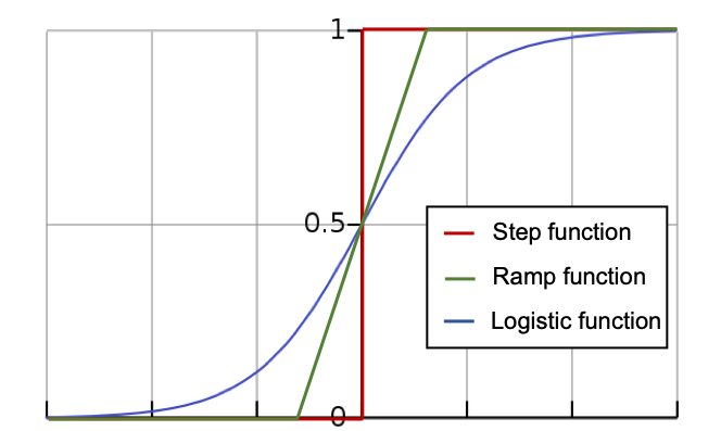
Figure 1: The step function and its surrogates.

We note that our structural lemma (showing that any stationary point of a non-convex surrogate suffices) crucially leverages the underlying distributional assumptions (i.e., the fact that $\mathcal{D}_{\mathbf{x}}$ is $(U,R)$ bounded). It follows from a lower bound construction in [DGT19] that the approach of the current paper does not extend to the distribution-independent setting. In particular, for any loss function $\mathcal{L}$, [DGT19] constructs examples where there exist stationary points of $\mathcal{L}$ defining hypotheses that are far from the target halfspace.

1.4 Related and Prior Work

Prior Work on Learning with Massart Noise

We start with a summary of prior work on distribution-specific PAC learning of halfspaces with Massart noise. The study of this learning problem was initiated in [ABHU15]. That work gave the first polynomial-time algorithm for the problem that succeeds under the uniform distribution on the unit sphere, assuming the upper bound on the noise rate $\eta$ is smaller than a sufficiently small constant ($\approx 10^{-6}$). Subsequently, [ABHZ16] gave a learning algorithm with sample and computational complexity $d^{2^{\mathrm{poly}(1/(1-2\eta))}}/\mathrm{poly}(\epsilon)$ that succeeds for any noise rate $\eta<1/2$ under any log-concave distribution.

The approach in [ABHU15, ABHZ16] uses an iterative localization-based method. These algorithms operate in a sequence of phases and it is shown that they make progress in each phase. To achieve this, [ABHU15, ABHZ16] leverage a distribution-specific agnostic learner for halfspaces [KKMS08] and develop sophisticated tools to control the trajectory of their algorithm.

Inspired by the localization approach, [YZ17] gave a perceptron-like algorithm (with sample complexity linear in $d$) for learning halfspaces with Massart noise under the uniform distribution on the sphere. Their algorithm again proceeds in phases and crucially exploits the symmetry of the uniform distribution to show that the angle between the current hypothesis $\widehat{\mathbf{w}}^{(i)}$ and the target halfspace $\mathbf{w}^{\ast}$ decreases in every phase. [ZLC17] also gave a polynomial-time algorithm for learning halfspaces with Massart noise under the uniform distribution on the unit sphere. Their algorithm works in the strong Massart noise model and is based on the Stochastic Gradient Langevin Dynamics (SGLD) algorithm applied to a smoothed version of the empirical $0-1$ loss. Their method leads to sample complexity $\Omega_{\eta}(d^{4}/\epsilon^{4})$ and its running time involves $\Omega_{\eta}(d^{13.5}/\epsilon^{16})$ inner product evaluations. More recently, [MV19] improved these bounds to $\Omega_{\eta}(d^{8.2}/\epsilon^{11.4})$ inner product evaluations via a similar approach. Our method is much simpler in comparison, running SGD directly on the population loss and using one sample per iteration with a significantly improved sample complexity and running time.

Furthermore, in contrast to the aforementioned approaches, we study a more general setting (in the sense that our method works for a broad family of distributions), and our approach is not tied to the iterations of any particular algorithm. Our structural lemma (Lemma 3.3) shows that any approximate stationary point of our non-convex surrogate loss suffices. As a consequence, one can apply any first-order method that converges to stationarity (and in particular vanilla SGD with projection on the unit sphere works). The upshot is that we do not need to establish guarantees for the trajectory of the method used to reach such a stationary point. The only thing that matters is the endpoint of the algorithm. Intriguingly, for a generic distribution in the class we consider, it is unclear if it is possible to establish a monotonicity property for a first-order method reaching a stationary point.

We note that the $d$-dependence in the sample complexity of our algorithm is information-theoretically optimal, even under Gaussian marginals. The $\epsilon$-dependence seems tight for our approach, given recent lower bounds for the convergence of SGD [DS19], or any stochastic first-order method [ACD⁺19], to stationary points of smooth non-convex functions.

Finally, we comment on the relation to a recent work on distribution-independent PAC learning of halfspaces with Massart noise [DGT19]. [DGT19] gave a distribution-independent PAC learner for halfspaces with Massart noise that approximates the target halfspace within misclassification error $\approx\eta$, i.e., it does not yield an arbitrarily close approximation to the true function. In contrast, the aforementioned distribution-specific algorithms achieve information-theoretically optimal misclassification error, which implies that the output hypothesis can be arbitrarily close to the true target halfspace. As a result, the results of this paper are not subsumed by [DGT19].

Comparison to RCN and Agnostic Settings

It is instructive to compare the complexity of learning halfspaces in the Massart model with two related noise models. In the RCN model, a polynomial-time algorithm is known in the distribution-independent PAC model [BFKV96, BFKV97]. In sharp contrast, even weak agnostic learning is hard in the distribution-independent setting [GR06, FGKP06, Dan16]. Moreover, obtaining information-theoretically optimal error guarantees remains computationally hard in the agnostic model, even when the marginal distribution is the standard Gaussian [KK14] (assuming the hardness of noisy parity). On the other hand, recent work [ABL17, DKS18] has given efficient algorithms (for Gaussian and log-concave marginals) with error $O(\mathrm{OPT})+\epsilon$, where $\mathrm{OPT}$ is the misclassification error of the optimal halfspace.

2 Preliminaries

For $n\in\mathbb{Z}_{+}$, let $[n]\stackrel{{\scriptstyle{\mathrm{\footnotesize def}}}}{{=}}\{1,\ldots,n\}$. We will use small boldface characters for vectors. For $\mathbf{x}\in\mathbb{R}^{d}$ and $i\in[d]$, $\mathbf{x}_{i}$ denotes the $i$-th coordinate of $\mathbf{x}$, and $\|\mathbf{x}\|_{2}\stackrel{{\scriptstyle{\mathrm{\footnotesize def}}}}{{=}}(\mathop{\textstyle\sum}_{i=1}^{d}\mathbf{x}_{i}^{2})^{1/2}$ denotes the $\ell_{2}$-norm of $\mathbf{x}$. We will use $\langle\mathbf{x},\mathbf{y}\rangle$ for the inner product of $\mathbf{x},\mathbf{y}\in\mathbb{R}^{d}$ and $\theta(\mathbf{x},\mathbf{y})$ for the angle between $\mathbf{x},\mathbf{y}$.

Let $\mathbf{e}_{i}$ be the $i$-th standard basis vector in $\mathbb{R}^{d}$. For $d\in\mathbb{N}$, let $\mathbb{S}^{d-1}\stackrel{{\scriptstyle{\mathrm{\footnotesize def}}}}{{=}}\{\mathbf{x}\in\mathbb{R}^{d}:\|\mathbf{x}\|_{2}=1\}$. Let $\mathrm{proj}_{U}(\mathbf{x})$ be the projection of $\mathbf{x}$ to subspace $U\subset\mathbb{R}^{d}$ and $U^{\perp}$ be its orthogonal complement.

Let $\operatorname*{\mathbf{E}}[X]$ denote the expectation of random variable $X$ and $\mathbf{Pr}[\mathcal{E}]$ the probability of event $\mathcal{E}$.

An (origin-centered) halfspace is any Boolean-valued function $h_{\mathbf{w}}:\mathbb{R}^{d}\to\{\pm 1\}$ of the form $h_{\mathbf{w}}(\mathbf{x})=\mathrm{sign}\left(\langle\mathbf{w},\mathbf{x}\rangle\right)$, where $\mathbf{w}\in\mathbb{R}^{d}$. (Note that we may assume w.l.o.g. that $\|\mathbf{w}\|_{2}=1$.)

We consider the binary classification setting where labeled examples $(\mathbf{x},y)$ are drawn i.i.d. from a distribution $\mathcal{D}$ on $\mathbb{R}^{d}\times\{\pm 1\}$. We denote by $\mathcal{D}_{\mathbf{x}}$ the marginal of $\mathcal{D}$ on $\mathbf{x}$. The misclassification error of a hypothesis $h:\mathbb{R}^{d}\to\{\pm 1\}$ (with respect to $\mathcal{D}$) is $\mathrm{err}_{0-1}^{\mathcal{D}}(h)\stackrel{{\scriptstyle{\mathrm{\footnotesize def}}}}{{=}}\mathbf{Pr}_{(\mathbf{x},y)\sim\mathcal{D}}[h(\mathbf{x})\neq y]$. The zero-one error between two functions $f,h$ (with respect to $\mathcal{D}_{\mathbf{x}}$) is $\mathrm{err}_{0-1}^{\mathcal{D}_{\mathbf{x}}}(f,h)\stackrel{{\scriptstyle{\mathrm{\footnotesize def}}}}{{=}}\mathbf{Pr}_{\mathbf{x}\sim\mathcal{D}_{\mathbf{x}}}[f(\mathbf{x})\neq h(\mathbf{x})]$.

We will use the following simple claim relating the zero-one loss between two halfspaces (with respect to a bounded distribution) and the angle between their normal vectors (see Appendix A.2 for the proof).

Claim 2.1.

Let $\mathcal{D}_{\mathbf{x}}$ be a $(U,R)$-bounded distribution on $\mathbb{R}^{d}$. For any $\mathbf{u},\mathbf{v}\in\mathbb{R}^{d}$ we have that $R^{2}/U\cdot\theta(\mathbf{u},\mathbf{v})\leq\mathrm{err}_{0-1}^{\mathcal{D}_{\mathbf{x}}}(h_{\mathbf{u}},h_{\mathbf{v}})$. Moreover, if $\mathcal{D}_{\mathbf{x}}$ is $(U,R,t(\cdot))$-bounded, for any $0<\epsilon\leq 1$, we have that $\mathrm{err}_{0-1}^{\mathcal{D}_{\mathbf{x}}}(h_{\mathbf{u}},h_{\mathbf{v}})\leq Ut(\epsilon)^{2}\cdot\theta(\mathbf{v},\mathbf{u})+\epsilon\;.$

3 Main Structural Result: Stationary Points Suffice

In this section, we prove our main structural result. In Section 3.1, we define a simple non-convex surrogate by replacing the step function by the (piecewise linear) ramp function and show that any approximate stationary point of this surrogate loss suffices. In Section 3.2, we prove our actual structural result for a smooth (sigmoid-based) approximation to the step function.

3.1 Warm-up: Non-convex surrogate based on ramp function

The main point of this subsection is to illustrate the key properties of a non-convex surrogate loss that allows us to argue that the stationary points of this loss are close to the true halfspace $\mathbf{w}^{\ast}$. To this end, we consider the ramp function $r_{\sigma}(t)$ with parameter $\sigma>0$ – a piecewise linear approximation to the step function. The ramp function and its derivative are defined as follows:

$$r_{\sigma}(t)=\begin{cases}0,&\text{for }t<-\sigma/2\\ \frac{t}{\sigma}+\frac{1}{2},&|t|\leq\sigma/2\\ 1,&t>\sigma/2\\ \end{cases}\qquad\text{and}\qquad r_{\sigma}^{\prime}(t)=\frac{1}{\sigma}\mathds{1}\{|t|\leq\sigma/2\}\;.$$ (1)

Observe that as $\sigma$ approaches $0$, $r_{\sigma}$ approaches the step function. Using the ramp function, we define the following non-convex surrogate loss function

$$\mathcal{L}_{\sigma}^{\text{ramp}}(\mathbf{w})=\operatorname*{\mathbf{E}}_{(\mathbf{x},y)\sim\mathcal{D}}\left[r_{\sigma}\left(-y\frac{\left\langle\mathbf{w},\mathbf{x}\right\rangle}{\left\|\mathbf{w}\right\|_{2}}\right)\right]\;.$$ (2)

Figure 2: The sign of the two-dimensional gradient projection.

Figure 3: The “good” (blue) and “bad” (red) regions inside a band of size $\sigma$.

To simplify notation, we will denote the inner product of $\mathbf{x}$ and the normalized $\mathbf{w}$ as $\ell(\mathbf{w},\mathbf{x})=\frac{\left\langle\mathbf{w},\mathbf{x}\right\rangle}{\left\|\mathbf{w}\right\|_{2}}$. By a straightforward calculation (see Appendix A.1), we get that the gradient of the objective $\mathcal{L}_{\sigma}^{\text{ramp}}(\mathbf{w})$ is

$$\nabla_{\mathbf{w}}\mathcal{L}_{\sigma}^{\text{ramp}}(\mathbf{w}) =\operatorname*{\mathbf{E}}_{\mathbf{x}\sim\mathcal{D}_{\mathbf{x}}}\left[-r_{\sigma}^{\prime}\left(\ell(\mathbf{w},\mathbf{x})\right)\ \nabla_{\mathbf{w}}\ell(\mathbf{w},\mathbf{x})\ (1-2\eta(\mathbf{x}))\ \mathrm{sign}(\left\langle\mathbf{w}^{\ast},\mathbf{x}\right\rangle)\right]\;.$$ (3)

Our goal is to establish a claim along the following lines.

Claim 3.1 (Informal).

For every $\epsilon>0$ there exists $\sigma>0$ such that for any vector $\widehat{\mathbf{w}}$ with $\theta(\mathbf{w}^{\ast},\widehat{\mathbf{w}})>\epsilon$, it holds $\left\|\nabla_{w}\mathcal{L}_{\sigma}^{\text{ramp}}(\widehat{\mathbf{w}})\right\|_{2}\geq\epsilon$.

The contrapositive of this claim implies that for every $\epsilon$ we can tune the parameter $\sigma$ so that all points with sufficiently small gradient have angle at most $\epsilon$ with the optimal halfspace $\mathbf{w}^{\ast}$. This is a parameter distance guarantee that is easy to translate to missclafication error (using Claim 2.1).

Since it suffices to prove that the norm of the gradient of any “bad” hypothesis (i.e., one whose angle with the optimal is greater than $\epsilon$) is large, we can restrict our attention to any subspace and bound from below the norm of the gradient in that subspace. Let $V=\mathrm{span}(\mathbf{w}^{\ast},\mathbf{w})$ and note that the inner products $\left\langle\mathbf{w}^{\ast},\mathbf{x}\right\rangle$, $\left\langle\mathbf{w},\mathbf{x}\right\rangle$ do not change after the projection to this subspace. Write any point $\mathbf{x}\in\mathbb{R}^{d}$ as $\mathbf{v}+\mathbf{u}$, where $\mathbf{v}\in V$ is the projection of $\mathbf{x}$ onto $V$ and $\mathbf{u}\in V^{\perp}$. Now, for each $\mathbf{v}$, we pick the worst-case $\mathbf{u}$ (the one that minimizes the norm of the gradient). We set $\eta_{V}(\mathbf{v})=\eta_{V}(\mathbf{v}+\mathbf{u}(\mathbf{v}))$. Since $\eta(\mathbf{x})\leq\eta$ for all $\mathbf{x}$, we also have that $\eta_{V}(\mathbf{v})\leq\eta$, for all $\mathbf{v}\in V$. Therefore, we have

$$\left\|\nabla_{\mathbf{w}}\mathcal{L}_{\sigma}^{\text{ramp}}(\mathbf{w})\right\|_{2}\geq\left\|\mathrm{proj}_{V}\nabla_{\mathbf{w}}\mathcal{L}_{\sigma}^{\text{ramp}}(\mathbf{w})\right\|_{2}=\left\|\operatorname*{\mathbf{E}}_{(\mathbf{x},y)\sim\mathcal{D}_{V}}[\nabla_{\mathbf{w}}\mathcal{L}_{\sigma}^{\text{ramp}}(\mathbf{w})]\right\|_{2}\;.$$

Without loss of generality, assume that $\widehat{\mathbf{w}}=\mathbf{e}_{2}$ and $\mathbf{w}^{\ast}=-\sin\theta\cdot\mathbf{e}_{1}+\cos\theta\cdot\mathbf{e}_{2}$, see Figure 3. To simplify notation, in what follows we denote by $\eta(\mathbf{x})$ the function $\eta_{V}(\mathbf{x})$ after the projection. Observe that the gradient is always perpendicular to $\widehat{\mathbf{w}}=\mathbf{e}_{2}$ (this is also clear from the fact that $\mathcal{L}_{\sigma}^{\text{ramp}}(\mathbf{w})$ does not depend on the length of $\mathbf{w}$). Therefore,

$$\left\|\operatorname*{\mathbf{E}}_{(\mathbf{x},y)\sim\mathcal{D}_{V}}[\nabla_{\mathbf{w}}\mathcal{L}_{\sigma}^{\text{ramp}}(\widehat{\mathbf{w}})]\right\|_{2}=|\left\langle\nabla_{\mathbf{w}}\mathcal{L}_{\sigma}^{\text{ramp}}(\widehat{\mathbf{w}}),\mathbf{e}_{1}\right\rangle|=\left|\operatorname*{\mathbf{E}}_{\mathbf{x}\sim(\mathcal{D}_{\mathbf{x}})_{V}}[-r_{\sigma}^{\prime}(\mathbf{x}_{2})(1-2\eta(\mathbf{x}))\mathrm{sign}(\left\langle\mathbf{w}^{\ast},\mathbf{x}\right\rangle)\mathbf{x}_{1}]\right|\;.$$ (4)

We partition $\mathbb{R}^{2}$ in two regions according to the sign of the pointwise gradient

$$g(\mathbf{x})=-r_{\sigma}^{\prime}(\mathbf{x}_{2})(1-2\eta(\mathbf{x}))\mathrm{sign}(\left\langle\mathbf{w}^{\ast},\mathbf{x}\right\rangle)\mathbf{x}_{1}\;.$$

Let

$$G=\{\mathbf{x}\in\mathbb{R}^{2}:g(\mathbf{x})\geq 0\}=\{\mathbf{x}\in\mathbb{R}^{2}:\mathbf{x}_{1}\mathrm{sign}(\left\langle\mathbf{w}^{\ast},\mathbf{x}\right\rangle)\leq 0\}\;,$$

and let $G^{c}$ be its complement. See Figure 3 for an illustration. To give some intuition behind this definition, imagine we were using SGD in this $2$-dimensional setting, and at some step $t$ we have $\mathbf{w}^{(t)}=\widehat{\mathbf{w}}=\mathbf{e}_{2}$. We draw a sample $(\mathbf{x},y)$ from the distribution $\mathcal{D}$ and update the hypothesis. Then the expected update (with respect to the label $y$) is

$$\mathbf{w}^{(t+1)}=\mathbf{e}_{2}-\left\langle g(\mathbf{x}),\mathbf{e}_{1}\right\rangle\mathbf{e}_{1}\;.$$

Therefore, assuming that $\theta(\mathbf{w}^{\ast},\mathbf{e}_{2})\in(0,\pi/2)$, the “good” points (region $G$) are those that decrease the $\mathbf{e}_{1}$ component (i.e., rotate the hypothesis counter-clockwise) and the “bad” points (region $G^{c}$) are those that try to increase the $\mathbf{e}_{1}$ component (rotate the hypothesis clockwise); see Figure 3.

We are now ready to explain the main idea behind the choice of the ramp function $r_{\sigma}(t)$. Recall that the derivative of the ramp function is the (scaled) indicator of a band of size $\sigma/2$ around $0$, $r^{\prime}_{\sigma}(t)=(1/\sigma)\mathds{1}\{|t|\leq\sigma/2\}$. Therefore, the gradient of this loss function amplifies the contribution of points close to the current guess $\mathbf{w}$, that is, points inside the band $\mathds{1}\{|\mathbf{x}_{2}|\leq\sigma/2\}$ in our $2$-dimensional example of Figure 3. Assume for simplicity that the marginal distribution $\mathcal{D}_{\mathbf{x}}$ is the uniform distribution on the $2$-dimensional unit ball. Then, no matter how small the angle of the true halfspace and our guess $\theta(\mathbf{w}^{\ast},\widehat{\mathbf{w}})$ is, we can always pick $\sigma$ sufficiently small so that the contribution of the “good” points (blue region in Figure 3) is much larger than the contribution of the “bad” points (red region).

Crucial in this argument is the fact that the distribution is “well-behaved” in the sense that the probability of every region is related to its area. This is where Definition 1.2 comes into play. To bound from below the contribution of “good” points, we require the anti-anti-concentration property of the distribution, namely a lower bound on the density function (in some bounded radius). To bound from above the contribution of “bad” points, we need the anti-concentration property of Definition 1.2, namely that the density is bounded from above (recall that we wanted the probability of a region to be related to its area).

We are now ready to show that our ramp-based non-convex loss works for all distributions satisfying Definition 1.2. In the following lemma, we prove that we can tune the parameter $\sigma$ so that the stationary points of our non-convex loss are close to $\mathbf{w}^{\ast}$. The following lemma is a precise version of our initial informal goal, Claim 3.1.

Lemma 3.2 (Stationary points of $\mathcal{L}_{\sigma}^{\text{ramp}}$ suffice).

Let $\mathcal{D}_{\mathbf{x}}$ be a $(U,R)$-bounded distribution on $\mathbb{R}^{d}$, and $\eta<1/2$ be an upper bound on the Massart noise rate. Fix any $\theta\in(0,\pi/2)$. Let $\mathbf{w}^{\ast}\in\mathbb{S}^{d-1}$ be the normal vector to the optimal halfspace and $\widehat{\mathbf{w}}\in\mathbb{S}^{d-1}$ be such that $\theta(\widehat{\mathbf{w}},\mathbf{w}^{\ast})\in(\theta,\pi-\theta)$. For $\sigma\leq\frac{R}{2U}\sqrt{1-2\eta}\sin\theta$, we have that $\left\|\nabla_{\mathbf{w}}\mathcal{L}_{\sigma}^{\text{ramp}}(\widehat{\mathbf{w}})\right\|_{2}\geq(1/8)R^{2}(1-2\eta)/U$.

Proof.

We will continue using the notation introduced in the above discussion. We let $V$ be the $2$-dimensional subspace spanned by $\mathbf{w}^{\ast}$ and $\widehat{\mathbf{w}}$. To simplify notation, we again assume without loss of generality that $\mathbf{w}^{\ast}=-\sin\theta\ \mathbf{e}_{1}+\cos\theta\ \mathbf{e}_{2}$ and $\widehat{\mathbf{w}}=\mathbf{e}_{2}$, see Figure 3. Using the triangle inequality and Equation (4), we obtain

$$\left\|\operatorname*{\mathbf{E}}_{(\mathbf{x},y)\sim\mathcal{D}_{V}}[\nabla_{\mathbf{w}}\mathcal{L}_{\sigma}^{\text{ramp}}(\widehat{\mathbf{w}})]\right\|_{2} \geq\operatorname*{\mathbf{E}}_{\mathbf{x}\sim(\mathcal{D}_{\mathbf{x}})_{V}}\left[r_{\sigma}^{\prime}(\mathbf{x}_{2})(1-2\eta(\mathbf{x}))|\mathbf{x}_{1}|\mathds{1}_{G}(\mathbf{x})\right]-\operatorname*{\mathbf{E}}_{\mathbf{x}\sim(\mathcal{D}_{\mathbf{x}})_{V}}\left[r_{\sigma}^{\prime}(\mathbf{x}_{2})(1-2\eta(\mathbf{x}))|\mathbf{x}_{1}|\mathds{1}_{\mathbf{x}\in G^{c}}\right]$$

$$=\operatorname*{\mathbf{E}}_{\mathbf{x}\sim(\mathcal{D}_{\mathbf{x}})_{V}}\left[r_{\sigma}^{\prime}(\mathbf{x}_{2})(1-2\eta(\mathbf{x}))|\mathbf{x}_{1}|\right]-2\operatorname*{\mathbf{E}}_{\mathbf{x}\sim(\mathcal{D}_{\mathbf{x}})_{V}}\left[r_{\sigma}^{\prime}(\mathbf{x}_{2})(1-2\eta(\mathbf{x}))|\mathbf{x}_{1}|\mathds{1}_{\mathbf{x}\in G^{c}}\right]\;.$$ (5)

We now bound from below the first term, as follows

$$\operatorname*{\mathbf{E}}_{\mathbf{x}\sim(\mathcal{D}_{\mathbf{x}})_{V}}\left[r_{\sigma}^{\prime}(\mathbf{x}_{2})(1-2\eta(\mathbf{x}))|\mathbf{x}_{1}|\right] \geq(1-2\eta)\operatorname*{\mathbf{E}}_{\mathbf{x}\sim(\mathcal{D}_{\mathbf{x}})_{V}}\left[\frac{\mathds{1}\{|\mathbf{x}_{2}|\leq\sigma/2\}}{\sigma}|\mathbf{x}_{1}|\right]$$

$$\geq\frac{(1-2\eta)R}{2\sqrt{2}\sigma}\operatorname*{\mathbf{E}}_{\mathbf{x}\sim(\mathcal{D}_{\mathbf{x}})_{V}}\left[\mathds{1}\left\{|\mathbf{x}_{2}|\leq\frac{\sigma}{2},\ \frac{R}{2\sqrt{2}}\leq|\mathbf{x}_{1}|\leq\frac{R}{\sqrt{2}}\right\}\right]$$

$$\geq\frac{(1-2\eta)R}{2\sqrt{2}\sigma}\cdot\frac{R\sigma}{\sqrt{2}U}=\frac{R^{2}}{4U}(1-2\eta),$$ (6)

where the first inequality follows from the upper bound on the noise $\eta(\mathbf{x})\leq\eta$, and the third one from the lower bound on the $2$-dimensional density function $1/U$ inside the ball $\left\|\mathbf{x}\right\|_{2}\leq R$ (see Definition 1.2).

We next bound from above the second term of Equation (5), that is the contribution of “bad” points. We have that

$$\operatorname*{\mathbf{E}}_{\mathbf{x}\sim(\mathcal{D}_{\mathbf{x}})_{V}}\left[r_{\sigma}^{\prime}(\mathbf{x}_{2})(1-2\eta(\mathbf{x}))|\mathbf{x}_{1}|\mathds{1}_{\mathbf{x}\in G^{c}}\right] \leq\operatorname*{\mathbf{E}}_{\mathbf{x}\sim(\mathcal{D}_{\mathbf{x}})_{V}}\left[\frac{\mathds{1}\{|\mathbf{x}_{2}|\leq\sigma/2\}}{\sigma}|\mathbf{x}_{1}|\mathds{1}\{\mathbf{x}\in G^{c}\}\right]$$

$$\leq\frac{1}{\sigma}\operatorname*{\mathbf{E}}_{\mathbf{x}\sim(\mathcal{D}_{\mathbf{x}})_{V}}\left[|\mathbf{x}_{1}|\mathds{1}\{\mathbf{x}\in G^{c},|\mathbf{x}_{2}|\leq\sigma/2\}\right]\;.$$

We now observe that for $\theta\in(0,\pi/2]$ it holds

$$G^{c}=\{\mathbf{x}:\mathbf{x}_{1}\mathrm{sign}(\left\langle\mathbf{w}^{\ast},\mathbf{x}\right\rangle)>0\}=\{\mathbf{x}:\mathbf{x}_{1}\mathrm{sign}(-\mathbf{x}_{1}\sin\theta+\mathbf{x}_{2}\cos\theta)>0\}\subseteq\{\mathbf{x}:\mathbf{x}_{1}\mathbf{x}_{2}>0\}\;.$$

On the other hand, if $\theta\in(\pi/2,\pi]$ we have $G^{c}\subseteq\{\mathbf{x}:\mathbf{x}_{1}\mathbf{x}_{2}<0\}$. Assume first that $\theta\in(0,\pi/2]$ (the same argument works also for the other case). Then the intersection of the band $\{\mathbf{x}:|\mathbf{x}_{2}|\leq\sigma/2\}$ and $G^{c}$ is contained in the union of two rectangles ${\cal R}=\{\mathbf{x}:|\mathbf{x}_{1}|\leq\sigma/(2\tan\theta),\ |\mathbf{x}_{2}|\leq\sigma/2,\ \mathbf{x}_{1}\mathbf{x}_{2}>0\}$, see Figure 3. Therefore,

$$\operatorname*{\mathbf{E}}_{\mathbf{x}\sim(\mathcal{D}_{\mathbf{x}})_{V}}\left[r_{\sigma}^{\prime}(\mathbf{x}_{2})(1-2\eta(\mathbf{x}))|\mathbf{x}_{1}|\mathds{1}_{\mathbf{x}\in G^{c}}\right] \leq\frac{1}{\sigma}\frac{\sigma}{2\tan\theta}\operatorname*{\mathbf{E}}_{\mathbf{x}\sim(\mathcal{D}_{\mathbf{x}})_{V}}\left[\mathds{1}\{\mathbf{x}\in G^{c},|\mathbf{x}_{1}|\leq\frac{\sigma}{2\tan\theta},|\mathbf{x}_{2}|\leq\frac{\sigma}{2}\}\right]$$

$$\leq\frac{1}{\sigma}\frac{\sigma}{2\tan\theta}\operatorname*{\mathbf{E}}_{\mathbf{x}\sim(\mathcal{D}_{\mathbf{x}})_{V}}\left[\mathds{1}\{\mathbf{x}\in R\}\right]\leq\frac{1}{2\tan\theta}\cdot\frac{U\sigma^{2}}{2\tan\theta}$$

$$\leq\frac{R^{2}}{16U}(1-2\eta)\;,$$ (7)

where for the last inequality we used our assumption that $\sigma\leq\frac{R}{2U}\sqrt{1-2\eta}\sin\theta$. To finish the proof, we substitute the bounds (3.1), (7) in Equation (5). ∎

3.2 Main structural result: Non-convex surrogate via smooth approximation

In this subsection, we prove the structural result that is required for the correctness of our efficient gradient-descent algorithm in the following section. We consider the non-convex surrogate loss

$$\mathcal{L}_{\sigma}(\mathbf{w})=\operatorname*{\mathbf{E}}_{(\mathbf{x},y)\sim\mathcal{D}}\left[S_{\sigma}\left(-y\frac{\left\langle\mathbf{w},\mathbf{x}\right\rangle}{\left\|\mathbf{w}\right\|_{2}}\right)\right],$$ (8)

where $S_{\sigma}(t)=\frac{1}{1+e^{-t/\sigma}}$ is the logistic function with growth rate $1/\sigma$. That is, we have replaced the step function by the sigmoid. As $\sigma\to 0$, $S_{\sigma}(t)$ approaches the step function. Formally, we prove the following:

Lemma 3.3 (Stationary points of $\mathcal{L}_{\sigma}$ suffice).

Let $\mathcal{D}_{\mathbf{x}}$ be a $(U,R)$-bounded distribution on $\mathbb{R}^{d}$, and $\eta<1/2$ be an upper bound on the Massart noise rate. Fix any $\theta\in(0,\pi/2)$. Let $\mathbf{w}^{\ast}\in\mathbb{S}^{d-1}$ be the normal vector to the optimal halfspace and $\widehat{\mathbf{w}}\in\mathbb{S}^{d-1}$ be such that $\theta(\widehat{\mathbf{w}},\mathbf{w}^{\ast})\in(\theta,\pi-\theta)$. For $\sigma\leq\frac{R}{8U}\sqrt{1-2\eta}\sin\theta$, we have that $\left\|\nabla_{\mathbf{w}}\mathcal{L}_{\sigma}(\widehat{\mathbf{w}})\right\|_{2}\geq\frac{1}{32U}R^{2}(1-2\eta)$.

The proof of Lemma 3.3 is conceptually similar to the proof of Lemma 3.2 for the ramp function given in the previous subsection. The main difference is that, in the smoothed setting, it is harder to bound the contribution of each region of Figure 3 and the calculations end-up being more technical.

Proof of Lemma 3.3.

Figure 4: The “good” (blue) and “bad” (red) regions.

Without loss of generality, we will assume that $\widehat{\mathbf{w}}=\mathbf{e}_{2}$ and $\mathbf{w}^{\ast}=-\sin\theta\cdot\mathbf{e}_{1}+\cos\theta\cdot\mathbf{e}_{2}$. Using the same argument as in the proof of Section 3.1, we let $V=\mathrm{span}(\mathbf{w}^{\ast},\mathbf{w})$ and have

$$\left\|\operatorname*{\mathbf{E}}_{(\mathbf{x},y)\sim\mathcal{D}_{V}}[\nabla_{\mathbf{w}}\mathcal{L}_{\sigma}(\widehat{\mathbf{w}})]\right\|_{2}=\left|\operatorname*{\mathbf{E}}_{\mathbf{x}\sim(\mathcal{D}_{\mathbf{x}})_{V}}[-S^{\prime}_{\sigma}(|\mathbf{x}_{2}|)(1-2\eta(\mathbf{x}))\mathrm{sign}(\left\langle\mathbf{w}^{\ast},\mathbf{x}\right\rangle)\mathbf{x}_{1}]\right|\;.$$ (9)

We partition $\mathbb{R}^{2}$ in two regions according to the sign of the gradient. Let

$$G=\{(\mathbf{x}_{1},\mathbf{x}_{2})\in\mathbb{R}^{2}:\mathbf{x}_{1}\mathrm{sign}(\left\langle\mathbf{w}^{\ast},\mathbf{x}\right\rangle)>0\}\;,$$

and let $G^{c}$ be its complement. Using the triangle inequality and Equation (9), we obtain

$$\left\|\operatorname*{\mathbf{E}}_{(\mathbf{x},y)\sim\mathcal{D}_{V}}[\nabla_{\mathbf{w}}\mathcal{L}_{\sigma}(\widehat{\mathbf{w}})]\right\|_{2} \geq\operatorname*{\mathbf{E}}_{\mathbf{x}\sim(\mathcal{D}_{\mathbf{x}})_{V}}\left[S^{\prime}_{\sigma}(|\mathbf{x}_{2}|)(1-2\eta(\mathbf{x}))|\mathbf{x}_{1}|\mathds{1}_{G}(\mathbf{x})\right]-\operatorname*{\mathbf{E}}_{\mathbf{x}\sim(\mathcal{D}_{\mathbf{x}})_{V}}\left[S^{\prime}_{\sigma}(|\mathbf{x}_{2}|)(1-2\eta(\mathbf{x}))|\mathbf{x}_{1}|\mathds{1}_{G^{c}}(\mathbf{x})\right]$$

$$\geq\frac{(1-2\eta)}{4}\operatorname*{\mathbf{E}}_{\mathbf{x}\sim(\mathcal{D}_{\mathbf{x}})_{V}}\left[\frac{e^{-|\mathbf{x}_{2}|/\sigma}}{\sigma}\cdot|\mathbf{x}_{1}|\cdot\mathds{1}_{G}(\mathbf{x})\right]-\operatorname*{\mathbf{E}}_{\mathbf{x}\sim(\mathcal{D}_{\mathbf{x}})_{V}}\left[\frac{e^{-|\mathbf{x}_{2}|/\sigma}}{\sigma}\cdot|\mathbf{x}_{1}|\cdot\mathds{1}_{G^{c}}(\mathbf{x})\right]\;,$$ (10)

where we used the upper bound on the Massart noise rate $\eta(\mathbf{x})\leq\eta$ and the fact that the sigmoid $S_{\sigma}(|t|)^{2}$ is bounded from above by $1$ and bounded from below by $1/4$.

We can now bound each term separately using the fact that the distribution is $(U,R)$-bounded. Assume first that $\theta(\mathbf{w}^{\ast},\widehat{\mathbf{w}})=\theta\in(0,\pi/2)$. Then we can express the region in polar coordinates as $G=\{(r,\phi):\phi\in(0,\theta)\cup(\pi/2,\pi+\theta)\cup(3\pi/2,2\pi)\}$. See Figure 4 for an illustration.

We denote by $\gamma(x,y)$ the density of the $2$-dimensional projection on $V$ of the marginal distribution $\mathcal{D}_{\mathbf{x}}$. Since the integral is non-negative, we can bound from below the contribution of region $G$ on the gradient by integrating over $\phi\in(\pi/2,\pi)$. Specifically, we have:

$$\operatorname*{\mathbf{E}}_{\mathbf{x}\sim(\mathcal{D}_{\mathbf{x}})_{V}}\left[\frac{e^{-|\mathbf{x}_{2}|/\sigma}}{\sigma}\ |\mathbf{x}_{1}|\ \mathds{1}_{G}(\mathbf{x})\right] \geq\int_{0}^{\infty}\int_{\pi/2}^{\pi}\gamma(r\cos\phi,r\sin\phi)r^{2}|\cos\phi|\frac{e^{-\frac{r\sin{\phi}}{\sigma}}}{\sigma}\mathrm{d}\phi\mathrm{d}r$$

$$=\int_{0}^{\infty}\int_{0}^{\pi/2}\gamma(r\cos\phi,r\sin\phi)r^{2}\cos\phi\frac{e^{-\frac{r\sin{\phi}}{\sigma}}}{\sigma}\mathrm{d}\phi\mathrm{d}r$$

$$\geq\frac{1}{U}\int_{0}^{R}r^{2}\mathrm{d}r\int_{0}^{\pi/2}\cos\phi\frac{e^{-\frac{R\sin{\phi}}{\sigma}}}{\sigma}\mathrm{d}\phi$$

$$=\frac{1}{3U}R^{2}\left(1-e^{-\frac{R}{\sigma}}\right)\geq\frac{1}{3U}R^{2}\left(1-e^{-8}\right)\;,$$ (11)

where for the second inequality we used the lower bound $1/U$ on the density function $\gamma(x,y)$ (see Definition 1.2) and for the last inequality we used that $\sigma\leq\frac{R}{8}$.

We next bound from above the contribution of the gradient in region $G^{c}$. Note that $G^{c}=\{(r,\phi):\phi\in B_{\theta}=(\pi/2-\theta,\pi/2)\cup(3\pi/2-\theta,3\pi/2)\}$. Hence, we can write:

$$\operatorname*{\mathbf{E}}_{\mathbf{x}\sim(\mathcal{D}_{\mathbf{x}})_{V}}\left[\frac{e^{-|\mathbf{x}_{2}|/\sigma}}{\sigma}\ |\mathbf{x}_{1}|\ \mathds{1}_{G^{c}}(\mathbf{x})\right] =\int_{0}^{\infty}\int_{\phi\in B_{\theta}}\gamma(r\cos\phi,r\sin\phi)r^{2}\cos{\phi}e^{-\frac{r\sin{\phi}}{\sigma}}\mathrm{d}\phi\mathrm{d}r$$

$$\leq\frac{2U}{\sigma}\int_{0}^{\infty}\int_{\theta}^{\pi/2}r^{2}\cos{\phi}e^{-\frac{r\sin{\phi}}{\sigma}}\mathrm{d}\phi\mathrm{d}r$$

$$=\frac{2U\sigma^{2}\cos^{2}\theta}{\sin^{2}\theta}$$

$$=\frac{(1-2\eta)R^{2}}{32U}\cos^{2}\theta\;,$$ (12)

where the inequality follows from the upper bound $U$ on the density $\gamma(x,y)$ (see Definition 1.2) and the last inequality follows from our assumption that $\sigma\leq\frac{R}{8U}\sqrt{1-2\eta}\sin(\theta)$. Combining (11) and (12), we have

$$\operatorname*{\mathbf{E}}_{\mathbf{x}\sim(\mathcal{D}_{\mathbf{x}})_{V}}\left[\frac{e^{-|\mathbf{x}_{2}|/\sigma}}{\sigma}\ |\mathbf{x}_{1}|\ \mathds{1}_{G^{c}}(\mathbf{x})\right] \leq\frac{(1-2\eta)R^{2}}{32U}\cos^{2}\theta$$

$$\leq\frac{(1-2\eta)R^{2}\left(1-e^{-8}\right)}{24U}$$

$$\leq\frac{1}{2}\frac{(1-2\eta)}{4}\operatorname*{\mathbf{E}}_{\mathbf{x}\sim(\mathcal{D}_{\mathbf{x}})_{V}}\left[\frac{e^{-|\mathbf{x}_{2}|/\sigma}}{\sigma}\ |\mathbf{x}_{1}|\ \mathds{1}_{G}(\mathbf{x})\right]\;,$$ (13)

where the second inequality follows from $\cos^{2}\theta\leq 1$ and $\frac{1}{32}\leq\frac{\left(1-e^{-8}\right)}{24}$. Using (13) in (10), we obtain

$$\left\|\operatorname*{\mathbf{E}}_{(\mathbf{x},y)\sim\mathcal{D}_{V}}\left[\nabla_{\mathbf{w}}\mathcal{L}_{\sigma}(\widehat{\mathbf{w}})\right]\right\|_{2}\geq\frac{1}{2}\frac{(1-2\eta)}{4}\operatorname*{\mathbf{E}}_{\mathbf{x}\sim(\mathcal{D}_{\mathbf{x}})_{V}}\left[\frac{e^{-|\mathbf{x}_{2}|/\sigma}}{\sigma}\ |\mathbf{x}_{1}|\ \mathds{1}_{G}(\mathbf{x})\right]\geq\frac{1}{32U}(1-2\eta)\ R^{2}\;.$$

To conclude the proof, notice that the case where $\theta(\widehat{\mathbf{w}},\mathbf{w}^{\ast})\in(\pi/2,\pi-\theta)$ follows similarly. Finally, in the case where $\theta=\pi/2$, the region $G^{c}$ is empty, and we again get the same lower bound on the gradient. This completes the proof of Lemma 3.3. ∎

4 Main Algorihtmic Result: Proof of Theorem 1.3

In this section, we prove our main algorithmic result, which we restate below:

Theorem 4.1.

Let $\mathcal{D}$ be a distribution on $\mathbb{R}^{d}\times\{-1,+1\}$ such that the marginal $\mathcal{D}_{\mathbf{x}}$ on $\mathbb{R}^{d}$ is $(U,R,t())$-bounded. Let $\eta<1/2$ be an upper bound on the Massart noise rate. Algorithm 2 has the following performance guarantee: It draws $m=O\left((U/R)^{12}\cdot t^{8}(\epsilon/2)/(1-2\eta)^{10}\right)\cdot O(d/\epsilon^{4})$ labeled examples from $\mathcal{D}$, uses $O(m)$ gradient evaluations, and outputs a hypothesis vector $\bar{\mathbf{w}}$ that satisfies $\mathrm{err}_{0-1}^{\mathcal{D}_{\mathbf{x}}}(h_{\bar{\mathbf{w}}},f)\leq\epsilon$ with probability at least $1-\delta$, where $f$ is the target halfspace.

Our algorithm proceeds by Projected Stochastic Gradient Descent (PSGD), with projection on the $\ell_{2}$-unit sphere, to find an approximate stationary point of our non-convex surrogate loss. Since $\mathcal{L}_{\sigma}(\mathbf{w})$ is non-smooth for vectors $\mathbf{w}$ close to $\mathbf{0}$, at each step, we project the update on the unit sphere to avoid the region where the smoothness parameter is high.

Recall that a function $f:\mathbb{R}^{d}\mapsto\mathbb{R}$ is called $L$-Lipschitz if there is a parameter $L>0$ such that $\left\|f(\mathbf{x})-f(\mathbf{y})\right\|_{2}\leq L\left\|\mathbf{x}-\mathbf{y}\right\|_{2}$ for all $\mathbf{x},\mathbf{y}\in\mathbb{R}^{d}$. We will make use of the following folklore result on the convergence of projected SGD (for completeness, we provide a proof in Appendix B.1).

Algorithm 1 PSGD for $f(\mathbf{w})=\operatorname*{\mathbf{E}}_{\mathbf{z}\sim\mathcal{D}}[g(\mathbf{z},\mathbf{w})]$

1:procedure psgd($f,T,\beta$) $\triangleright$ $f(\mathbf{w})=\operatorname*{\mathbf{E}}_{\mathbf{z}\sim\mathcal{D}}[g(\mathbf{z},\mathbf{w})]$: loss, $T$: number of steps, $\beta$: step size.

2:     ${\mathbf{w}}^{(0)}\leftarrow\mathbf{e}_{1}$

3:     for $i=1,\dots,T$ do

4:       Sample $\mathbf{z}^{(i)}$ from $\mathcal{D}$.

5:       ${\mathbf{v}}^{(i)}\leftarrow{\mathbf{w}}^{(i-1)}-\beta\nabla_{\mathbf{w}}g({\mathbf{z}}^{(i)},{\mathbf{w}}^{(i-1)})$

6:       ${\mathbf{w}}^{(i)}\leftarrow{\mathbf{v}}^{(i)}/\left\|{\mathbf{v}}^{(i)}\right\|_{2}$

7:     return $({\mathbf{w}}^{(1)},\ldots,{\mathbf{w}}^{(T)})$.

lem:PSGD[PSGD] Let $f:\mathbb{R}^{d}\mapsto\mathbb{R}$ with $f(\mathbf{w})=\operatorname*{\mathbf{E}}_{\mathbf{z}\sim\mathcal{D}}[g(\mathbf{z},\mathbf{w})]$ for some function $g:\mathbb{R}^{d}\times\mathbb{R}^{d}\mapsto\mathbb{R}$. Assume that for any vector $\mathbf{w}$, $g(\cdot,\mathbf{w})$ is positive homogeneous of degree-$0$ on $\mathbf{w}$. Let $\mathcal{W}=\{\mathbf{w}\in\mathbb{R}^{d}:\left\|\mathbf{w}\right\|_{2}\geq 1\}$ and assume that $f,g$ are continuously differentiable functions on $\mathcal{W}$. Moreover, assume that $|f(\mathbf{w})|\leq R$, $\nabla_{\mathbf{w}}f(\mathbf{w})$ is $L$-Lipschitz on $\mathcal{W}$, $\operatorname*{\mathbf{E}}_{\mathbf{z}\sim\mathcal{D}}\left[\left\|\nabla_{\mathbf{w}}g(\mathbf{z},\mathbf{w})\right\|_{2}^{2}\right]\leq B$ for all $\mathbf{w}\in\mathcal{W}$. After $T$ iterations the output $({\mathbf{w}}^{(1)},\ldots,{\mathbf{w}}^{(T)})$ of Algorithm 1 satisfies

$$\operatorname*{\mathbf{E}}_{{\mathbf{z}}^{(1)},\ldots,{\mathbf{z}}^{(T)}\sim\mathcal{D}}\left[\frac{1}{T}\sum_{i=1}^{T}\left\|\nabla_{\mathbf{w}}f({\mathbf{w}}^{(i)})\right\|_{2}^{2}\right]\leq\sqrt{\frac{LBR}{2T}}\;.$$

If, additionally, $\left\|\operatorname*{\mathbf{E}}_{\mathbf{z}\sim\mathcal{D}}[\nabla_{\mathbf{w}}g(\mathbf{z},\mathbf{w})]\right\|_{2}^{2}\leq C$ for all $\mathbf{w}\in\mathcal{W}$, we have that with $T=(2LBR+8C^{2}\log(1/\delta))/\epsilon^{4}$ it holds $\min_{i=1,\ldots,T}\left\|\nabla_{\mathbf{w}}f(\mathbf{w}^{(i)})\right\|_{2}\leq\epsilon,$ with probability at least $1-\delta$.

We will require the following lemma establishing the smoothness properties of our loss (based on $S_{\sigma}$). See Appendix B.2 for the proof.

lem:sigmoid_smoothness[Sigmoid Smoothness] Let $S_{\sigma}(t)=1/(1+e^{-t/\sigma})$ and $\mathcal{L}_{\sigma}(\mathbf{w})=\operatorname*{\mathbf{E}}_{(\mathbf{x},y)\sim\mathcal{D}}\left[S_{\sigma}\left(-y\frac{\left\langle\mathbf{w},\mathbf{x}\right\rangle}{\left\|\mathbf{w}\right\|_{2}}\right)\right]$, for $\mathbf{w}\in{\cal W}$, where ${\cal W}=\{\mathbf{w}\in\mathbb{R}^{d}:\left\|\mathbf{w}\right\|_{2}\geq 1\}$. We have that $\mathcal{L}_{\sigma}(\mathbf{w})$ is continuously differentiable in ${\cal W}$, $|\mathcal{L}_{\sigma}(\mathbf{w})|\leq 1$, $\operatorname*{\mathbf{E}}_{(\mathbf{x},y)\sim\mathcal{D}}[\left\|\nabla_{{\mathbf{w}}}S_{\sigma}({\mathbf{w}},\mathbf{x},y)\right\|_{2}^{2}]\leq 4d/\sigma^{2}$, $\left\|\nabla_{\mathbf{w}}\mathcal{L}_{\sigma}(\mathbf{w})\right\|_{2}^{2}\leq 4/\sigma^{2}$, and $\nabla_{\mathbf{w}}\mathcal{L}_{\sigma}(\mathbf{w})$ is $(6/\sigma+12/\sigma^{2})$-Lipschitz.

Putting everything together gives Theorem 4.1.

Algorithm 2 Learning Halfspaces with Massart Noise

1:procedure Alg($\epsilon$, $U$, $R$, $t(\cdot)$)

2:     $C_{1}\leftarrow\Theta(U^{12}/R^{12})$.

3:     $C_{2}\leftarrow\Theta(R/U^{2})$.

4:     $T\leftarrow C_{1}\ d\ t(\epsilon/2)^{8}/(\epsilon^{4}(1-2\eta)^{10})\log(1/\delta)$. $\triangleright$ number of steps

5:     $\beta\leftarrow C_{2}^{2}\ d(1-2\eta)^{3}\epsilon^{2}/(t(\epsilon/2)^{4}T^{1/2})$. $\triangleright$ step size

6:     $\sigma\leftarrow C_{2}\ \sqrt{1-2\eta}\ \epsilon/t^{2}(\epsilon/2)$.

7:     $({\mathbf{w}}^{(0)},{\mathbf{w}}^{(1)},\ldots,{\mathbf{w}}^{(T)})\leftarrow\mathrm{PSGD}(f,T,\beta)$. $\triangleright$ $f(\mathbf{w})=\operatorname*{\mathbf{E}}_{(\mathbf{x},y)\sim\mathcal{D}}\left[S_{\sigma}\Big{(}-y\frac{\left\langle\mathbf{w},\mathbf{x}\right\rangle}{\left\|\mathbf{w}\right\|_{2}}\Big{)}\right]$, (1)

8:     $L\leftarrow\{\pm{\mathbf{w}}^{(i)}\}_{i\in[T]}$. $\triangleright$ $L$: List of candidate vectors

9:     Draw $N=O(\log(T/\delta)/(\epsilon^{2}(1-2\eta)^{2}))$ samples from $\mathcal{D}$.

10:     $\bar{\mathbf{w}}\leftarrow\operatorname*{argmin}_{\mathbf{w}\in L}\sum_{j=1}^{N}\mathds{1}\{\mathrm{sign}(\left\langle\mathbf{w},\mathbf{x}^{(j)}\right\rangle)\neq y^{(j)}\}$.

11:     return $\bar{\mathbf{w}}$.

Proof of Theorem 4.1.

By Claim 2.1, to guarantee $\mathrm{err}_{0-1}^{\mathcal{D}_{\mathbf{x}}}(h_{\bar{\mathbf{w}}},f)\leq\epsilon$ it suffices to show that the angle $\theta(\bar{\mathbf{w}},\mathbf{\mathbf{w}^{\ast}})\leq O(\epsilon(1-2\eta)/(Ut^{2}(\epsilon/2)))=:\theta_{0}$. Using (the contrapositive of) Lemma 3.3, we get that with $\sigma=\Theta((R/U)\sqrt{1-2\eta}\theta_{0})$, if the norm squared of the gradient of some vector $\mathbf{w}\in\mathbb{S}^{d-1}$ is smaller than $\rho=O((R^{2}/U)(1-2\eta))$, then $\mathbf{w}$ is close to either $\mathbf{\mathbf{w}^{\ast}}$ or $-\mathbf{\mathbf{w}^{\ast}}$ – that is, $\theta(\mathbf{w},\mathbf{\mathbf{w}^{\ast}})\leq\theta_{0}$ – or $\theta(\mathbf{w},-\mathbf{\mathbf{w}^{\ast}})\leq\theta_{0}$. Therefore, it suffices to find a point $\mathbf{w}$ with gradient $\left\|\nabla_{\mathbf{w}}\mathcal{L}_{\sigma}(\mathbf{w})\right\|_{2}\leq\rho$.

From Lemma LABEL:lem:sigmoid_smoothness, we have that our PSGD objective function is bounded above by $1$,

$$\operatorname*{\mathbf{E}}\left[\left\|\nabla_{\mathbf{w}}S_{\sigma}\Big{(}-y\frac{\left\langle\mathbf{w},\mathbf{x}\right\rangle}{\left\|\mathbf{w}\right\|_{2}}\Big{)}\right\|_{2}^{2}\right]\leq O(d/\sigma^{2})\;,$$

$\left\|\operatorname*{\mathbf{E}}\left[\nabla_{\mathbf{w}}S_{\sigma}\Big{(}-y\frac{\left\langle\mathbf{w},\mathbf{x}\right\rangle}{\left\|\mathbf{w}\right\|_{2}}\Big{)}\right]\right\|_{2}^{2}\leq O(1/\sigma^{2})$, and that the gradient is Lipschitz with Lipschitz constant $O(1/\sigma^{2})$. Using these bounds for the parameters of Lemma LABEL:lem:PSGD, we get that with $T=O(\frac{d}{\sigma^{4}\rho^{4}}\log(1/\delta))$ steps, the norm of the gradient of some vector in the list $({\mathbf{w}}^{(0)},\ldots,{\mathbf{w}}^{(T)})$ will be at most $\rho$ with probability $1-\delta$. Therefore, the required number of iterations is

$$T=O\left(d\frac{U^{12}}{R^{12}}\frac{t^{8}(\epsilon/2)\log(1/\delta)}{\epsilon^{4}(1-2\eta)^{10}}\right)\;.$$

We know that one of the hypotheses in the list $L$ (line 8 of Algorithm 2) is $\epsilon$-close to the true $\mathbf{\mathbf{w}^{\ast}}$. We can evaluate all of them on a small number of samples from the distribution $\mathcal{D}$ to obtain the best among them. From Hoeffding’s inequality, it follows that $N=O(\log(T/\delta)/(\epsilon^{2}(1-2\eta)^{2}))$ samples are sufficient to guarantee that the excess error of the chosen hypothesis is at most $\epsilon(1-2\eta)$. Using Fact A.1, for any hypotheses $h$, and the target concept $f$, it holds $\mathrm{err}_{0-1}^{\mathcal{D}_{\mathbf{x}}}(h,f)\leq\frac{1}{(1-2\eta)}(\mathrm{err}_{0-1}^{\mathcal{D}}(h)-\mathrm{OPT}),$ and therefore the chosen hypothesis achieves error at most $2\epsilon$. This completes the proof of Theorem 4.1. ∎

5 Strong Massart Noise Model

We start by defining the strong Massart noise model, which was considered in [ZLC17] for the special case of the uniform distribution on the sphere. The main difference with the standard Massart noise model is that, in the strong model, the noise rate is allowed to approach arbitrarily close to $1/2$ for points that lie very close to the separating hyperplane.

Definition 5.1 (Distribution-specific PAC Learning with Strong Massart Noise).

Let $\mathcal{C}$ be the concept class of halfspaces over $X=\mathbb{R}^{d}$, $\mathcal{F}$ be a known family of structured distributions on $X$, $0<c\leq 1$ and $0<\epsilon<1$. Let $f(\mathbf{x})=\mathrm{sign}(\left\langle\mathbf{\mathbf{w}^{\ast}},\mathbf{x}\right\rangle)$ be an unknown target function in $\mathcal{C}$. A noisy example oracle, $\mathrm{EX}^{\mathrm{SMas}}(f,\mathcal{F},\eta)$, works as follows: Each time $\mathrm{EX}^{\mathrm{SMas}}(f,\mathcal{F},\eta)$ is invoked, it returns a labeled example $(\mathbf{x},y)$, such that: (a) $\mathbf{x}\sim\mathcal{D}_{\mathbf{x}}$, where $\mathcal{D}_{\mathbf{x}}$ is a fixed distribution in $\mathcal{F}$, and (b) $y=f(\mathbf{x})$ with probability $1-\eta(\mathbf{x})$ and $y=-f(\mathbf{x})$ with probability $\eta(\mathbf{x})$, for an unknown parameter $\eta(\mathbf{x})\leq\max\{1/2-c|\left\langle\mathbf{\mathbf{w}^{\ast}},\mathbf{x}\right\rangle|,0\}$. Let $\mathcal{D}$ denote the joint distribution on $(\mathbf{x},y)$ generated by the above oracle. A learning algorithm is given i.i.d. samples from $\mathcal{D}$ and its goal is to output a hypothesis $h$ such that with high probability the misclassification error of $h$ is $\epsilon$-close to the misclassfication error of $f$, i.e., it holds $\mathrm{err}_{0-1}^{\mathcal{D}}(h)\leq\mathrm{err}_{0-1}^{\mathcal{D}}(f)+\epsilon$.

The main result of this section is the following theorem:

Theorem 5.2 (Learning Halfspaces with Strong Massart Noise).

Let $\mathcal{D}$ be a distribution on $\mathbb{R}^{d}\times\{\pm 1\}$ such that the marginal $\mathcal{D}_{\mathbf{x}}$ on $\mathbb{R}^{d}$ is $(U,R,t())$-bounded. Let $0<c<1$ be the parameter of the strong Massart noise model. Algorithm 3 has the following performance guarantee: It draws $m=O\left((U^{12}/R^{18})(t^{8}(\epsilon/2)/c^{6})\right)O(d/\epsilon^{4})$ labeled examples from $\mathcal{D}$, uses $O(m)$ gradient evaluations, and outputs a hypothesis vector $\bar{\mathbf{w}}$ that satisfies $\mathrm{err}_{0-1}^{\mathcal{D}}(h_{\bar{\mathbf{w}}})\leq\mathrm{err}_{0-1}^{\mathcal{D}}(f)+\epsilon$ with probability at least $1-\delta$.

The proof of Theorem 5.2 follows along the same lines as in the previous sections. We show that any stationary point of our non-convex surrogate suffices and then use projected SGD.

The main structural result of this section generalizes Lemma 3.3:

Lemma 5.3 (Stationary points of $\mathcal{L}_{\sigma}$ suffice with strong Massart noise).

Let $\mathcal{D}_{\mathbf{x}}$ be a $(U,R)$-bounded distribution on $\mathbb{R}^{d}$, and let $c\in(0,1)$ be the parameter of strong Massart noise model. Let $\theta\in(0,\pi/2)$. Let $\mathbf{\mathbf{w}^{\ast}}\in\mathbb{S}^{d-1}$ be the normal vector to an optimal halfspace and $\widehat{\mathbf{w}}\in\mathbb{S}^{d-1}$ be such that $\theta(\widehat{\mathbf{w}},\mathbf{\mathbf{w}^{\ast}})\in(\theta,\pi-\theta)$. For $\sigma\leq\frac{R}{24U}\sqrt{cR}\sin(\theta)$, we have $\left\|\nabla_{\mathbf{w}}\mathcal{L}_{\sigma}(\widehat{\mathbf{w}})\right\|_{2}\geq\frac{1}{288U}c\ R^{3}.$

Proof.

Without loss of generality, we can assume that $\widehat{\mathbf{w}}=\mathbf{e}_{2}$ and $\mathbf{w}^{\ast}=-\sin\theta\cdot\mathbf{e}_{1}+\cos\theta\cdot\mathbf{e}_{2}$. Using the same argument as in the Section 3, for $V=\mathrm{span}(\mathbf{w}^{\ast},\mathbf{w})$, we have

$$\left\|\operatorname*{\mathbf{E}}_{(\mathbf{x},y)\sim\mathcal{D}_{V}}[\nabla_{\mathbf{w}}\mathcal{L}_{\sigma}(\widehat{\mathbf{w}})]\right\|_{2}=|\left\langle\nabla_{\mathbf{w}}\mathcal{L}_{\sigma}(\widehat{\mathbf{w}}),\mathbf{e}_{1}\right\rangle|=\left|\operatorname*{\mathbf{E}}_{\mathbf{x}\sim\mathcal{D}_{\mathbf{x}}}[-S^{\prime}_{\sigma}(|\mathbf{x}_{2}|)(1-2\eta(\mathbf{x}))\mathrm{sign}(\left\langle\mathbf{w}^{*},\mathbf{x}\right\rangle)\mathbf{x}_{1}]\right|$$ (14)

We partition $\mathbb{R}^{2}$ in two regions according to the sign of the gradient. Let $G=\{(\mathbf{x}_{1},\mathbf{x}_{2})\in\mathbb{R}^{2}:\mathbf{x}_{1}\mathrm{sign}(\left\langle\mathbf{w}^{*},\mathbf{x}\right\rangle)>0\}$, and let $G^{c}$ be its complement. Using the triangle inequality and Equation (14) we obtain

$$\left\|\operatorname*{\mathbf{E}}_{(\mathbf{x},y)\sim\mathcal{D}_{V}}[\nabla_{\mathbf{w}}\mathcal{L}_{\sigma}(\widehat{\mathbf{w}})]\right\|_{2} \geq\operatorname*{\mathbf{E}}_{\mathbf{x}\sim\mathcal{D}_{\mathbf{x}}}[S^{\prime}_{\sigma}(|\mathbf{x}_{2}|)(1-2\eta(\mathbf{x}))|\mathbf{x}_{1}|\mathds{1}_{G}(\mathbf{x})]-\operatorname*{\mathbf{E}}_{\mathbf{x}\sim\mathcal{D}_{\mathbf{x}}}[S^{\prime}_{\sigma}(|\mathbf{x}_{2}|)(1-2\eta(\mathbf{x}))|\mathbf{x}_{1}|\mathds{1}_{G^{c}}(\mathbf{x})]$$

$$\geq\frac{1}{4}\operatorname*{\mathbf{E}}_{\mathbf{x}\sim\mathcal{D}_{\mathbf{x}}}\left[(1-2\eta(\mathbf{x}))\frac{e^{-|\mathbf{x}_{2}|/\sigma}}{\sigma}\ |\mathbf{x}_{1}|\ \mathds{1}_{G}(\mathbf{x})\right]-\operatorname*{\mathbf{E}}_{\mathbf{x}\sim\mathcal{D}_{\mathbf{x}}}\left[\frac{e^{-|\mathbf{x}_{2}|/\sigma}}{\sigma}\ |\mathbf{x}_{1}|\ \mathds{1}_{G^{c}}(\mathbf{x})\right]\;,$$ (15)

where we used the fact that the sigmoid $S_{\sigma}(|t|)^{2}$ is upper bounded by $1$ and lower bounded by $1/4$.

We can now bound each term using the fact that the distribution is $(U,R)$-bounded. Assume first that $\theta(\mathbf{w}^{*},\mathbf{w})=\theta\in(0,\pi/2)$. Then, (see Figure 3) we can express region $G$ in polar coordinates as $G=\{(r,\phi):\phi\in(0,\theta)\cup(\pi/2,\pi+\theta)\cup(3\pi/2,2\pi)\}$. We denote by $\gamma(x,y)$ the density of the $2$-dimensional projection on $V$ of the marginal distribution $\mathcal{D}_{\mathbf{x}}$. Since the integrand is non-negative we may bound from below the contribution of region $G$ on the gradient by integrating over $\phi\in(\pi/2,\pi)$.

$$\operatorname*{\mathbf{E}}_{\mathbf{x}\sim\mathcal{D}_{\mathbf{x}}}\left[(1-2\eta(\mathbf{x}))\frac{e^{-|\mathbf{x}_{2}|/\sigma}}{\sigma}\ |\mathbf{x}_{1}|\ \mathds{1}_{G}(\mathbf{x})\right] \geq\int_{0}^{\infty}\int_{\pi/2}^{\pi}(1-2\eta(\mathbf{x}))\gamma(r\cos\phi,r\sin\phi)r^{2}|\cos\phi|\frac{e^{-\frac{r\sin{\phi}}{\sigma}}}{\sigma}\mathrm{d}\phi\mathrm{d}r$$ (16)

$$=\int_{0}^{\infty}\int_{0}^{\pi/2}(1-2\eta(\mathbf{x}))\gamma(r\cos\phi,r\sin\phi)r^{2}\cos\phi\frac{e^{-\frac{r\sin{\phi}}{\sigma}}}{\sigma}\mathrm{d}\phi\mathrm{d}r$$

$$\geq\int_{R/2}^{R}\int_{0}^{\pi/2}c|\left\langle\mathbf{w}^{\ast},\mathbf{x}\right\rangle|\gamma(r\cos\phi,r\sin\phi)r^{2}\cos\phi\frac{e^{-\frac{r\sin{\phi}}{\sigma}}}{\sigma}\mathrm{d}\phi\mathrm{d}r$$

$$\geq c\frac{R}{6}\int_{R/2}^{R}\int_{0}^{\pi/2}\gamma(r\cos\phi,r\sin\phi)r^{2}\cos\phi\frac{e^{-\frac{r\sin{\phi}}{\sigma}}}{\sigma}\mathrm{d}\phi\mathrm{d}r$$

$$\geq c\frac{R}{6U}\int_{R/2}^{R}r^{2}\mathrm{d}r\int_{0}^{\pi/2}\cos\phi\frac{e^{-\frac{R\sin{\phi}}{\sigma}}}{\sigma}\mathrm{d}\phi$$

$$=c\frac{7}{144U}R^{3}\left(1-e^{-\frac{R}{\sigma}}\right)\geq c\frac{7}{144U}R^{3}\left(1-e^{-8}\right)\;,$$ (17)

where for the third inequality we used that for $\left\|\mathbf{x}\right\|_{2}\geq R/2$, we have that $\left\langle\mathbf{w}^{\ast},\mathbf{x}\right\rangle=\frac{R}{2}(\cos(\theta)+\sin(\theta))\geq R/6$, for the fourth inequality we used the lower bound $1/U$ on the density function $\gamma(r\cos\phi,r\sin\phi)$ (see Definition 1.2), and for the last inequality we used that $\sigma\leq R/8$.

We next bound from above the contribution of the gradient of region $G^{c}$. We have $G^{c}=\{(r,\phi):\phi\in B_{\theta}=(\pi/2-\theta,\pi/2)\cup(3\pi/2-\theta,3\pi/2)\}$

$$\operatorname*{\mathbf{E}}_{\mathbf{x}\sim\mathcal{D}_{\mathbf{x}}}\left[\frac{e^{-|\mathbf{x}_{2}|/\sigma}}{\sigma}\ |\mathbf{x}_{1}|\ \mathds{1}_{G^{c}}(\mathbf{x})\right] =\int_{0}^{\infty}\int_{\phi\in B_{\theta}}\gamma(r\cos\phi,r\sin\phi)r^{2}\cos\phi e^{-\frac{r\sin{\phi}}{\sigma}}\mathrm{d}\phi\mathrm{d}r\$$

$$\leq\frac{2U}{\sigma}\int_{0}^{\infty}\int_{\theta}^{\pi/2}r^{2}\cos\phi e^{-\frac{r\sin{\phi}}{\sigma}}\mathrm{d}\phi\mathrm{d}r$$

$$=\frac{2U\sigma^{2}\cos^{2}\theta}{\sin^{2}\theta}=\frac{2R^{3}c\cos^{2}\theta}{24^{2}U}\;,$$ (18)

where the inequality follows from the upper bound $U$ on the density $\gamma(r\cos\phi,r\sin\phi)$ (see Definition 1.2), and the last equality follows from the value of $\sigma$. Combining (17) and (18), we have

$$\operatorname*{\mathbf{E}}_{\mathbf{x}\sim(\mathcal{D}_{\mathbf{x}})_{V}}\left[\frac{e^{-|\mathbf{x}_{2}|/\sigma}}{\sigma}\ |\mathbf{x}_{1}|\ \mathds{1}_{G^{c}}(\mathbf{x})\right] \leq\frac{2R^{3}c\cos^{2}\theta}{24^{2}U}$$

$$\leq\frac{1}{8}\frac{7cR^{3}\left(1-e^{-8}\right)}{144U}$$

$$\leq\frac{1}{2}\frac{1}{4}\operatorname*{\mathbf{E}}_{\mathbf{x}\sim(\mathcal{D}_{\mathbf{x}})_{V}}\left[\frac{e^{-|\mathbf{x}_{2}|/\sigma}}{\sigma}\ |\mathbf{x}_{1}|\ \mathds{1}_{G}(\mathbf{x})\right]\;,$$ (19)

where the second inequality follows from the identity $\cos^{2}\theta\leq 1$ and $\frac{2}{24^{2}}\leq\frac{1}{8}\frac{7\left(1-e^{-8}\right)}{144}$. Using (19) in (15), we obtain

$$\left\|\operatorname*{\mathbf{E}}_{(\mathbf{x},y)\sim\mathcal{D}_{V}}[\nabla_{\mathbf{w}}\mathcal{L}_{\sigma}(\widehat{\mathbf{w}})]\right\|_{2}\geq\frac{1}{8}\operatorname*{\mathbf{E}}_{\mathbf{x}\sim(\mathcal{D}_{\mathbf{x}})_{V}}\left[\frac{e^{-|\mathbf{x}_{2}|/\sigma}}{\sigma}\ |\mathbf{x}_{1}|\ \mathds{1}_{G}(\mathbf{x})\right]\geq\frac{cR^{3}}{288U}\;.$$

To conclude the proof, notice that the case where $\theta(\mathbf{w},\mathbf{\mathbf{w}^{\ast}})\in(\pi/2,\pi-\theta)$ follows by an analogous argument. Finally, in the case where $\theta=\pi/2$, the region $G^{c}$ is empty and we can again get the same lower bound on the gradient norm.

∎

Algorithm 3 Learning Halfspaces with Strong Massart Noise

1:procedure Alg($\epsilon$, $U$, $R$, $t(\cdot)$)

2:     $C_{1}\leftarrow\Theta(U^{12}/R^{18})$.

3:     $C_{2}\leftarrow\Theta(R^{3/2}/U^{2})$.

4:     $T\leftarrow C_{1}\ d\ t(\epsilon/2)^{8}/(\epsilon^{4}c^{6})\log(1/\delta)$. $\triangleright$ number of steps

5:     $\beta\leftarrow C_{2}^{2}\ d\ c^{3}\epsilon^{2}/(t(\epsilon/2)^{4}T^{1/2})$.

6:     $\sigma\leftarrow C_{2}\ c^{1/2}\ \epsilon/t^{2}(\epsilon/2)$.

7:     $({\mathbf{w}}^{(0)},{\mathbf{w}}^{(1)},\ldots,{\mathbf{w}}^{(T)})\leftarrow\mathrm{PSGD}(f,T,\beta)$. $\triangleright$ $f(\mathbf{w})=\operatorname*{\mathbf{E}}_{(\mathbf{x},y)\sim\mathcal{D}}\left[S_{\sigma}\Big{(}-y\frac{\left\langle\mathbf{w},\mathbf{x}\right\rangle}{\left\|\mathbf{w}\right\|_{2}}\Big{)}\right]$, (1)

8:     $L\leftarrow\{\pm{\mathbf{w}}^{(i)}\}_{i\in[T]}$. $\triangleright$ $L$: List of candinate vectors

9:     Draw $N=O(\log(T/\delta)/\epsilon^{2})$ samples from $\mathcal{D}$.

10:     $\bar{\mathbf{w}}\leftarrow\operatorname*{argmin}_{\mathbf{w}\in L}\sum_{j=1}^{N}\mathds{1}\{\mathrm{sign}(\left\langle\mathbf{w},\mathbf{x}^{(j)}\right\rangle)\neq y^{(j)}\}$.

11:     return $\bar{\mathbf{w}}$.

Proof of Theorem 5.2.

From Claim 2.1, we have that to make the $\mathrm{err}_{0-1}^{\mathcal{D}_{\mathbf{x}}}(h_{\bar{\mathbf{w}}},f)\leq\epsilon$ it suffices to prove that the angle $\theta(\bar{\mathbf{w}},\mathbf{\mathbf{w}^{\ast}})\leq O(\epsilon/(Ut^{2}(\epsilon/2)))=:\theta$. Using (the contrapositive of) Lemma 5.3 we get that with $\sigma\leq\Theta(R/U\sqrt{cR}\theta)$, if the norm squared of the gradient of some vector $\mathbf{w}\in\mathbb{S}^{d-1}$ is smaller than $\rho=O(R^{3}c/U)$, then $\mathbf{w}$ is close to either $\mathbf{\mathbf{w}^{\ast}}$ or $-\mathbf{\mathbf{w}^{\ast}}$, that is $\theta(\mathbf{w},\mathbf{\mathbf{w}^{\ast}})\leq\theta$ or $\theta(\mathbf{w},-\mathbf{\mathbf{w}^{\ast}})\leq\theta$. Therefore, it suffices to find a point $\mathbf{w}$ with gradient $\left\|\nabla_{\mathbf{w}}\mathcal{L}_{\sigma}(\mathbf{w})\right\|_{2}\leq\rho\;.$

From Lemma LABEL:lem:sigmoid_smoothness, we have that our PSGD objective function $\mathcal{L}_{\sigma}(\mathbf{w})$, is bounded by $1$,

$$\operatorname*{\mathbf{E}}\left[\left\|\nabla_{\mathbf{w}}S_{\sigma}\Big{(}-y\frac{\left\langle\mathbf{w},\mathbf{x}\right\rangle}{\left\|\mathbf{w}\right\|_{2}}\Big{)}\right\|_{2}^{2}\right]\leq O(d/\sigma^{2})\;,$$

$\left\|\operatorname*{\mathbf{E}}\left[\nabla_{\mathbf{w}}S_{\sigma}\Big{(}-y\frac{\left\langle\mathbf{w},\mathbf{x}\right\rangle}{\left\|\mathbf{w}\right\|_{2}}\Big{)}\right]\right\|_{2}^{2}\leq O(1/\sigma^{2})$, and that the gradient of $\mathcal{L}_{\sigma}(\mathbf{w})$ is Lipschitz with Lipschitz constant $O(1/\sigma^{2})$. Using these bounds for the parameters of Lemma LABEL:lem:PSGD, we get that with $T=O(\frac{d}{\sigma^{4}\rho^{4}}\log(1/\delta))$ rounds, the norm of the gradient of some vector of the list $({\mathbf{w}}^{(0)},\ldots,{\mathbf{w}}^{(T)})$ will be at most $\rho$ with $1-\delta$ probability. Therefore, the required number of rounds is

$$T=O\left(\frac{U^{12}}{R^{18}}\frac{dt^{8}(\epsilon/2)\log(1/\delta)}{\epsilon^{4}c^{6}}\right)\;.$$

Now that we know that one of the hypotheses in the list $L$ (line 8 of Algorithm 3) is $\epsilon$-close to the true $\mathbf{\mathbf{w}^{\ast}}$, we can evaluate all of them on a small number of samples from the distribution $\mathcal{D}$ to obtain the best among them. The fact that $N=O(\log(T/\delta)/(\epsilon^{2}))$ samples are sufficient to guarantee that the excess error of the chosen hypothesis is at most $\epsilon$ with probability $1-\delta$ follows directly from Hoeffding’s inequality. This completes the proof. ∎

Appendix A Omitted Technical Lemmas

A.1 Formula for the Gradient

Recall that to simplify notation, we will write $\ell(\mathbf{w},\mathbf{x})=\frac{\left\langle\mathbf{w},\mathbf{x}\right\rangle}{\left\|\mathbf{w}\right\|_{2}}$. Note that $\nabla_{\mathbf{w}}\ell(\mathbf{w},\mathbf{x})=\frac{\mathbf{x}}{\left\|\mathbf{w}\right\|_{2}}-\left\langle\mathbf{w},\mathbf{x}\right\rangle\frac{\mathbf{w}}{\left\|\mathbf{w}\right\|_{2}^{3}}$. The gradient of the objective $\mathcal{L}_{\sigma}^{\text{ramp}}(\mathbf{w})$ is then

$$\nabla_{\mathbf{w}}\mathcal{L}_{\sigma}^{\text{ramp}}(\mathbf{w}) =\operatorname*{\mathbf{E}}_{(\mathbf{x},y)\sim\mathcal{D}}\left[-r_{\sigma}^{\prime}\left(-y\ \ell(\mathbf{w},\mathbf{x})\right)\nabla_{\mathbf{w}}\ell(\mathbf{w},\mathbf{x})\ y\right]$$

$$=\operatorname*{\mathbf{E}}_{(\mathbf{x},y)\sim\mathcal{D}}\left[-r_{\sigma}^{\prime}\left(\ell(\mathbf{w},\mathbf{x})\right)\ \nabla_{\mathbf{w}}\ell(\mathbf{w},\mathbf{x})\ y\right]$$

$$=\operatorname*{\mathbf{E}}_{\mathbf{x}\sim\mathcal{D}_{\mathbf{x}}}\left[-r_{\sigma}^{\prime}\left(\ell(\mathbf{w},\mathbf{x})\right)\ \nabla_{\mathbf{w}}\ell(\mathbf{w},\mathbf{x})\ (\mathrm{sign}(\left\langle\mathbf{w}^{\ast},\mathbf{x}\right\rangle)(1-\eta(\mathbf{x}))-\mathrm{sign}(\left\langle\mathbf{w}^{\ast},\mathbf{x}\right\rangle)\eta(\mathbf{x}))\right]$$

$$=\operatorname*{\mathbf{E}}_{\mathbf{x}\sim\mathcal{D}_{\mathbf{x}}}\left[-r_{\sigma}^{\prime}\left(\ell(\mathbf{w},\mathbf{x})\right)\ \nabla_{\mathbf{w}}\ell(\mathbf{w},\mathbf{x})\ (1-2\eta(\mathbf{x}))\ \mathrm{sign}(\left\langle\mathbf{w}^{\ast},\mathbf{x}\right\rangle)\right]\;,$$ (20)

where in the second equality we used that the $r_{\sigma}^{\prime}(t)$ is an even function.

A.2 Proof of Claim 2.1

The following claim relates the angle between two vectors and the zero-one loss between the corresponding halfspaces under bounded distributions.

Claim 2.1.

Let $\mathcal{D}_{\mathbf{x}}$ be a $(U,R)$-bounded distribution on $\mathbb{R}^{d}$. Then for any $\mathbf{u},\mathbf{v}\in\mathbb{R}^{d}$ we have

$$(R^{2}/U)\theta(\mathbf{u},\mathbf{v})\leq\mathrm{err}_{0-1}^{\mathcal{D}_{\mathbf{x}}}(h_{\mathbf{u}},h_{\mathbf{v}})\;.$$ (21)

Moreover, if $\mathcal{D}$ is $(U,R,t(\cdot))$-bounded, we have that for any $\epsilon\in(0,1]$

$$\mathrm{err}_{0-1}^{\mathcal{D}_{\mathbf{x}}}(h_{\mathbf{u}},h_{\mathbf{v}})\leq Ut(\epsilon)^{2}\theta(\mathbf{v},\mathbf{u})+\epsilon\;.$$ (22)

Proof.

Let $V$ be the subspace spanned by $\mathbf{v},\mathbf{u}$, and let $(\mathcal{D}_{\mathbf{x}})_{V}$ be the projection of $\mathcal{D}_{\mathbf{x}}$ onto $V$. Since $\left\langle\mathbf{v},\mathbf{x}\right\rangle=\left\langle\mathbf{v},\mathrm{proj}_{V}(\mathbf{x})\right\rangle$ and $\left\langle\mathbf{u},\mathbf{x}\right\rangle=\left\langle\mathbf{u},\mathrm{proj}_{V}(\mathbf{x})\right\rangle$ we have

$$\mathrm{err}_{0-1}^{\mathcal{D}_{\mathbf{x}}}(h_{\mathbf{u}},h_{\mathbf{v}}) =\mathrm{err}_{0-1}^{(\mathcal{D}_{\mathbf{x}})_{V}}(h_{\mathbf{u}},h_{\mathbf{v}})\;.$$

Without loss of generality, we can assume that $V=\mathrm{span}(\mathbf{e}_{1},\mathbf{e}_{2})$, where $\mathbf{e}_{1},\mathbf{e}_{2}$ are orthogonal vectors of $\mathbb{R}^{2}$. Then from Definition 1.2, using the fact that $1/U\leq f_{V}(\mathbf{x})$ for all $\mathbf{x}$ such that $\left\|\mathbf{x}\right\|_{\infty}\leq R$, which is also true for all $\mathbf{x}$ with $\left\|\mathbf{x}\right\|_{2}\leq R$, the above probability is bounded below by $\frac{R^{2}}{U}\theta(\mathbf{u},\mathbf{v})$, which proves (21). To prove (22), we observe that

$$\mathrm{err}_{0-1}^{(\mathcal{D}_{\mathbf{x}})_{V}}(h_{\mathbf{u}},h_{\mathbf{v}}) \leq\mathbf{Pr}_{\mathbf{x}\sim(\mathcal{D}_{\mathbf{x}})_{V}}[\mathrm{sign}(\left\langle\mathbf{u},\mathbf{x}\right\rangle)\neq\mathrm{sign}(\left\langle\mathbf{v},\mathbf{x}\right\rangle)\text{ and }\left\|\mathbf{x}\right\|_{2}\leq t(\epsilon)]+\mathbf{Pr}_{\mathbf{x}\sim(\mathcal{D}_{\mathbf{x}})_{V}}[\left\|\mathbf{x}\right\|_{2}\geq t(\epsilon)]$$

$$\leq Ut(\epsilon)^{2}\theta+\epsilon.$$

∎

A.3 Relation Between Misclassification Error and Error to Target Halfspace

The following well-known fact relates the misspecification error with respect to $\mathcal{D}$ and the zero-one loss with respect to the optimal halfspace. We include a proof for the sake of completeness.

Fact A.1.

Let $\mathcal{D}$ be a distribution on $\mathbb{R}^{d}\times\{\pm 1\}$, $\eta<1/2$ be an upper bound on the Massart noise rate. Then if $f(\mathbf{x})=\mathrm{sign}(\left\langle\mathbf{\mathbf{w}^{\ast}},\mathbf{x}\right\rangle)$ and $h(\mathbf{x})=\mathrm{sign}(\left\langle\mathbf{u},\mathbf{x}\right\rangle)$ we have

$$\mathrm{err}_{0-1}^{\mathcal{D}_{\mathbf{x}}}(h,f)\leq\frac{1}{1-2\eta}\left(\mathrm{err}_{0-1}^{\mathcal{D}}(h)-\mathrm{OPT}\right)\;.$$

Proof.

We have that

$$\mathrm{err}_{0-1}^{\mathcal{D}}(h)=\operatorname*{\mathbf{E}}_{(\mathbf{x},y)\sim\mathcal{D}}[\mathds{1}\{h(\mathbf{x})\neq f(\mathbf{x})\} =\operatorname*{\mathbf{E}}_{\mathbf{x}\sim\mathcal{D}_{\mathbf{x}}}[(1-\eta(\mathbf{x}))\mathds{1}\{h(\mathbf{x})\neq f(\mathbf{x})\}]+\operatorname*{\mathbf{E}}_{\mathbf{x}\sim\mathcal{D}_{\mathbf{x}}}[\eta(\mathbf{x})\mathds{1}\{h(\mathbf{x})=f(\mathbf{x})\}]$$

$$=\operatorname*{\mathbf{E}}_{\mathbf{x}\sim\mathcal{D}_{\mathbf{x}}}[(1-2\eta(\mathbf{x}))\mathds{1}\{h(\mathbf{x})\neq f(\mathbf{x})\}]+\operatorname*{\mathbf{E}}_{\mathbf{x}\sim\mathcal{D}_{\mathbf{x}}}[\eta(\mathbf{x})]$$

$$\geq\operatorname*{\mathbf{E}}_{\mathbf{x}\sim\mathcal{D}_{\mathbf{x}}}[(1-2\eta)\mathds{1}\{h(\mathbf{x})\neq f(\mathbf{x})\}]+\mathrm{OPT}$$

$$=(1-2\eta)\ \mathrm{err}_{0-1}^{\mathcal{D}_{\mathbf{x}}}(h,f)+\mathrm{OPT}\;,$$

where in the second inequality we used that $\eta(\mathbf{x})\leq\eta$ and $\operatorname*{\mathbf{E}}_{\mathbf{x}\sim\mathcal{D}_{\mathbf{x}}}[\eta(\mathbf{x})]=\mathrm{OPT}$. ∎

A.4 Log-concave and $s$-concave distributions are bounded

Lemma A.2 (Isotropic log-concave density bounds [LV07]).

Let $\gamma$ be the density of any isotropic log-concave distribution on $\mathbb{R}^{d}$. Then $\gamma(\mathbf{x})\geq 2^{-6d}$ for all $\mathbf{x}$ such that $0\leq\left\|\mathbf{x}\right\|_{2}\leq 1/9$. Furthermore, $\gamma(\mathbf{x})\leq\mathrm{e}\ 2^{8d}d^{d/2}$ for all $\mathbf{x}$.

We are also going to use the following concentration inequality providing sharp bounds on the tail probability of isotropic log-concave distributions.

Lemma A.3 (Paouris’ Inequality [Pao06]).

There exists an absolute constant $c>0$ such that if $\mathcal{D}_{\mathbf{x}}$ is any isotropic log-concave distribution on $\mathbb{R}^{d}$, then for all $t>1$ it holds

$$\operatorname*{\mathbf{Pr}}_{\mathbf{x}\sim\mathcal{D}_{\mathbf{x}}}[\left\|\mathbf{x}\right\|_{2}\geq ct\sqrt{d}]\leq\exp(-t\sqrt{d})\;.$$

Fact A.4.

An isotropic log-concave distribution on $\mathbb{R}^{d}$ is $(e2^{17},1/9,c\log(1/\epsilon)+2c)$-bounded, where $c>0$ is the absolute constant of Lemma A.3.

Proof.

Follows immediately from Lemma A.2, Lemma A.3, and the fact that the marginals of isotropic log-concave distributions are also isotropic log-concave. ∎

Now we are going to prove that $s$-concave are also $(U,R,t)$ bounded for all $s\geq-\frac{1}{2d+3}$. We will require the following lemma:

Lemma A.5 (Theorem 3 [BZ17]).

Let $\gamma(\mathbf{x})$ be an isotropic $s$-concave distribution density on $\mathbb{R}^{d}$, then the marginal on a subspace of $\mathbb{R}^{2}$ is $\frac{s}{1+(d-2)s}$-concave.

Lemma A.6 (Theorem 5 [BZ17]).

Let $\mathbf{x}$ come from an isotropic distribution over $\mathbb{R}^{d}$, with $s$-concave density. Then for every $t\geq 16$, we have

$$\mathbf{Pr}[\left\|\mathbf{x}\right\|_{2}>\sqrt{d}t]\leq\left(1-\frac{cst}{1+ds}\right)^{(1+ds)/s}\;,$$

where $c$ is an absolute constant.

Lemma A.7 (Theorem 9 [BZ17]).

Let $\gamma:\mathbb{R}^{d}\rightarrow\mathbb{R}_{+}$ be an isotropic $s$-concave density. Then

(a) Let $D(s,d)=(1+\alpha)^{-1/\alpha}\frac{1+3\beta}{3+3\beta}$, where $\beta=\frac{s}{1+(d-1)s}$, $\alpha=\frac{\beta}{1+\beta}$ and $\zeta=(1+\alpha)^{-\frac{1}{\alpha}}\frac{1+3\beta}{3+3\beta}$. For any $\mathbf{x}\in\mathbb{R}^{d}$ such that $\|\mathbf{x}\|\leq D(s,d)$, we have $\gamma(\mathbf{x})\geq\left(\frac{\|\mathbf{x}\|}{\zeta}((2-2^{-(d+1)s})^{-1}-1)+1\right)^{1/s}\gamma(0)$.

(b) $\gamma(\mathbf{x})\leq\gamma(0)\left[\left(\frac{1+\beta}{1+3\beta}\sqrt{3(1+\alpha)^{3/\alpha}}2^{d-1+1/s}\right)^{s}-1\right]^{1/s}$ for every $\mathbf{x}$.

(c) $(4e\pi)^{-d/2}\left[\left(\frac{1+\beta}{1+3\beta}\sqrt{3(1+\alpha)^{3/\alpha}}2^{d-1+\frac{1}{s}}\right)^{s}-1\right]^{-\frac{1}{s}}<\gamma(0)\leq(2-2^{-(d+1)s})^{1/s}\frac{d\Gamma(d/2)}{2\pi^{d/2}\zeta^{d}}$.

(d) $\gamma(\mathbf{x})\leq(2-2^{-(d+1)s})^{1/s}\frac{d\Gamma(d/2)}{2\pi^{d/2}\zeta^{d}}\left[\left(\frac{1+\beta}{1+3\beta}\sqrt{3(1+\alpha)^{3/\alpha}}2^{d-1+1/s}\right)^{s}-1\right]^{1/s}$ for every $\mathbf{x}$.

Lemma A.8.

Any isotropic $s$-concave distribution on $\mathbb{R}^{d}$ with $s\geq-\frac{1}{2d+3}$, is $\big{(}\Theta(1),\Theta(1),c/\epsilon^{1/6}\big{)}$-bounded where $c$ is an absolute constant.

Proof.

Set $\Gamma=\big{(}(\frac{1+2s}{1+4s}\sqrt{3(1+s/(1+2s))^{(3+6s)/s}}2^{1+1/s})^{s}-1\big{)}^{1/s}$. From Lemma A.7, we have

1. For any $\mathbf{x}\in\mathbb{R}^{2}$ such that $\left\|\mathbf{x}\right\|_{2}\leq(1+\frac{s}{1+2s})^{-\frac{1+2s}{s}}(\frac{1+4s}{3+6s})$, we have $\gamma(\mathbf{x})\geq\frac{1}{4e\pi\Gamma}$.

2. For any $\mathbf{x}\in\mathbb{R}^{2}$, we have: $\gamma(\mathbf{x})\leq\frac{(2^{3s+1}-1)^{1/s}(3+6s)^{2}\Gamma}{4\pi(1+4s)^{2}(\frac{1+3s}{1+2s})^{-\frac{1+2s}{s}}}$.

From Lemma A.5, we have that the marginals of an isotropic $s$-concave distribution on $\mathbb{R}^{d}$, on a $2$-dimensional subspace, are $s^{\prime}$-concave where $s^{\prime}=\frac{s}{1+(d-2)s}$. Using $s\geq-\frac{1}{2d+3}$, for $d\geq 3$, we have $s^{\prime}>-\frac{1}{8}$ and when $d=2$, we have $s^{\prime}=s\geq-1/7$. Thus, the value of $s^{\prime}$ is lower bounded by $-1/7$. To find the values $(U,R)$, we need to find a lower bound and an upper bound on density. From the expression of $\Gamma$, we observe that for $s^{\prime}\geq-1/7$ it holds $\Gamma<34\cdot 10^{3}$. Therefore, we obtain the following bounds

$$\gamma(\mathbf{x}) \geq\frac{1}{4e\pi\Gamma}>\frac{1}{10^{7}}\;,$$

$$R =\left(1+\frac{s^{\prime}}{1+2s^{\prime}}\right)^{-\frac{1+2s}{s^{\prime}}}\frac{1+4s^{\prime}}{3+6s^{\prime}}\geq 0.065\;,$$

$$\gamma(\mathbf{x}) \leq\frac{(2^{3s^{\prime}+1}-1)^{1/s^{\prime}}(3+6s^{\prime})^{2}\Gamma}{4\pi(1+4s^{\prime})^{2}(\frac{1+3s^{\prime}}{1+2s^{\prime}})^{-\frac{1+2s^{\prime}}{s^{\prime}}}}<3.3\cdot 10^{7}\;,$$

where we simplified each expression using the bounds of $s^{\prime}$. From Lemma A.6 we get tail bounds, by taking the appropriate $s^{\prime}$ that maximizes the error in the tail bound (which is $s^{\prime}=-1/7$). This completes the proof. ∎

Appendix B Omitted Proofs from Section 4

In Section B.1, we establish the convergence properties of projected SGD that we require. Even though this lemma should be folklore, we did not find an explicit reference. In Section B.2, we establish the smoothness of our non-convex surrogate function.

B.1 Proof of Lemma LABEL:lem:PSGD

For convenience, we restate the lemma here.

Lemma LABEL:lem:PSGD (PSGD).

Let $f:\mathbb{R}^{d}\mapsto\mathbb{R}$ with $f(\mathbf{w})=\operatorname*{\mathbf{E}}_{\mathbf{z}\sim\mathcal{D}}[g(\mathbf{z},\mathbf{w})]$ for some function $g:\mathbb{R}^{d}\times\mathbb{R}^{d}\mapsto\mathbb{R}$. Assume that for any vector $\mathbf{w}$, $g(\cdot,\mathbf{w})$ is positive homogeneous of degree-$0$ on $\mathbf{w}$. Let $\mathcal{W}=\{\mathbf{w}\in\mathbb{R}^{d}:\left\|\mathbf{w}\right\|_{2}\geq 1\}$ and assume that $f,g$ are continuously differentiable functions on $\mathcal{W}$. Moreover, assume that $|f(\mathbf{w})|\leq R$, $\nabla_{\mathbf{w}}f(\mathbf{w})$ is $L$-Lipschitz on $\mathcal{W}$, $\operatorname*{\mathbf{E}}_{\mathbf{z}\sim\mathcal{D}}\left[\left\|\nabla_{\mathbf{w}}g(\mathbf{z},\mathbf{w})\right\|_{2}^{2}\right]\leq B$ for all $\mathbf{w}\in\mathcal{W}$. After $T$ iterations the output $({\mathbf{w}}^{(1)},\ldots,{\mathbf{w}}^{(T)})$ of Algorithm 1 satisfies

$$\operatorname*{\mathbf{E}}_{{\mathbf{z}}^{(1)},\ldots,{\mathbf{z}}^{(T)}\sim\mathcal{D}}\left[\frac{1}{T}\sum_{i=1}^{T}\left\|\nabla_{\mathbf{w}}f({\mathbf{w}}^{(i)})\right\|_{2}^{2}\right]\leq\sqrt{\frac{LBR}{2T}}\;.$$

If, additionally, $\left\|\operatorname*{\mathbf{E}}_{\mathbf{z}\sim\mathcal{D}}[\nabla_{\mathbf{w}}g(\mathbf{z},\mathbf{w})]\right\|_{2}^{2}\leq C$ for all $\mathbf{w}\in\mathcal{W}$, we have that with $T=(2LBR+8C^{2}\log(1/\delta))/\epsilon^{4}$ it holds $\min_{i=1,\ldots,T}\left\|\nabla_{\mathbf{w}}f(\mathbf{w}^{(i)})\right\|_{2}\leq\epsilon,$ with probability at least $1-\delta$.

Proof.

Consider the update ${\mathbf{v}}^{(i)}={\mathbf{w}}^{(i-1)}-\beta\nabla g(\mathbf{z}^{(i)},\mathbf{w}^{(i-1)})$ at iteration $i$ of Algorithm 1. The projection step on the unit sphere (line 6 of Algorithm 1) ensures that $\left\|{\mathbf{w}}^{(i-1)}\right\|_{2}=1$. Observe that, since $g(\mathbf{z},{\mathbf{w}})$ is constant in the direction of ${\mathbf{w}}$, we have that $\nabla_{{\mathbf{w}}}g(\mathbf{z},\mathbf{w}^{(i-1)})$ is perpendicular to ${\mathbf{w}}^{(i-1)}$. Therefore, by the Pythagorean theorem, $\left\|{\mathbf{v}}^{(i)}\right\|_{2}^{2}=\left\|{\mathbf{w}}^{(i-1)}\right\|_{2}^{2}+\beta^{2}\left\|\nabla g(\mathbf{z}^{(i)},\mathbf{w}^{(i-1)})\right\|_{2}^{2}>1$ which implies that ${\mathbf{v}}^{(i)}\in{\cal W}$. Observe that the line that connects ${\mathbf{v}}^{(i)}$ and ${\mathbf{w}}^{(i-1)}$ is also contained in ${\cal W}$. Therefore, we have

$$f({\mathbf{v}}^{(i)})-f({\mathbf{w}}^{(i-1)}) =\left\langle\nabla_{{\mathbf{w}}}f({\mathbf{w}}^{(i-1)}),{\mathbf{v}}^{(i)}-{\mathbf{w}}^{(i-1)}\right\rangle$$

$$+\int_{0}^{1}\left\langle\nabla_{{\mathbf{w}}}f({\mathbf{w}}^{(i-1)}+t({\mathbf{v}}^{(i)}-{\mathbf{w}}^{(i-1)}))-\nabla_{{\mathbf{w}}}f({\mathbf{w}}^{(i-1)}),({\mathbf{v}}^{(i)}-{\mathbf{w}}^{(i-1)})\right\rangle\mathrm{d}t$$

$$\leq-\beta\left\langle\nabla f({\mathbf{w}}^{(i-1)}),\nabla_{{\mathbf{w}}}g(\mathbf{z}^{(i)},{\mathbf{w}}^{(i-1)})\right\rangle+\frac{\beta^{2}L}{2}\left\|\nabla_{{\mathbf{w}}}g(\mathbf{z}^{(i)},{\mathbf{w}}^{(i-1)})\right\|_{2}^{2}.$$

Observe now that, since $f$ does not depend on the length of its argument, we have $f({\mathbf{v}}^{(i)})=f({\mathbf{w}}^{(i)})$ and therefore

$$f({\mathbf{w}}^{(i)})-f({\mathbf{w}}^{(i-1)})\leq-\beta\left\langle\nabla f({\mathbf{w}}^{(i-1)}),\nabla_{{\mathbf{w}}}g(\mathbf{z}^{(i)},{\mathbf{w}}^{(i-1)})\right\rangle+\frac{\beta^{2}L}{2}\left\|\nabla_{{\mathbf{w}}}g(\mathbf{z}^{(i)},{\mathbf{w}}^{(i-1)})\right\|_{2}^{2}.$$

Conditioning on the previous samples $\mathbf{z}^{(1)},\ldots,\mathbf{z}^{(i-1)}$ we have

$$\operatorname*{\mathbf{E}}_{\mathbf{z}^{(i)}}[f({\mathbf{w}}^{(i)})-f({\mathbf{w}}^{(i-1)})|\mathbf{z}^{(1)},\ldots,\mathbf{z}^{(i-1)}] \leq\beta\left\|\nabla_{{\mathbf{w}}}f({\mathbf{w}}^{(i-1)})\right\|_{2}^{2}+\frac{\beta^{2}L}{2}\operatorname*{\mathbf{E}}_{\mathbf{z}^{(i)}}\left[\left\|\nabla_{{\mathbf{w}}}g(\mathbf{z}^{(i)},{\mathbf{w}}^{(i-1)})\right\|_{2}^{2}\right]$$

$$\leq-\beta\left\|\nabla_{{\mathbf{w}}}f({\mathbf{w}}^{(i-1)})\right\|_{2}^{2}+\frac{\beta^{2}LB}{2}.$$

Rearranging the above inequality, taking the average over $T$ iterations and using the law of total expectation, we obtain that by setting $\beta=\sqrt{2R/(LBT)}$. To get the high-probability version, we set

$$S_{T}(\mathbf{w}^{(1)},\ldots,\mathbf{w}^{(T)})=(1/T)\sum_{i=1}^{T}\left\|\nabla f(\mathbf{w}^{(i)})\right\|_{2}^{2}.$$

Notice that with $T=2LBR/\epsilon^{4}$ from the previous argument we obtain that $\operatorname*{\mathbf{E}}[S_{T}(\mathbf{w}^{(1)},\ldots,\mathbf{w}^{(T)})]\leq\epsilon^{2}/2$. Observe that

$$\left|S_{T}(\mathbf{w}^{(1)},\ldots,\mathbf{w}^{(i)},\ldots,\mathbf{w}^{(T)})-S_{T}(\mathbf{w}^{(1)},\ldots,{\mathbf{w}^{(i)}}^{\prime},\ldots,\mathbf{w}^{(T)})\right| \leq\frac{\left|\left\|\nabla f(\mathbf{w}^{(i)})\right\|_{2}^{2}-\left\|\nabla f({\mathbf{w}^{(i)}}^{\prime})\right\|_{2}^{2}\right|}{T}$$

$$\leq\frac{2C}{T}\;.$$

Lemma B.1 (Theorem 2.2 of [DL01]).

Suppose that $X_{1},\ldots X_{d}\in\cal X$ are independent random variables, and let $f:{\cal X}^{d}\mapsto\mathbb{R}$. Let $c_{1},\ldots,c_{n}$ satisfy

$$\sup_{x_{1},\ldots,x_{d},x_{i}^{\prime}}|f(x_{1},\ldots x_{i},\ldots x_{d})-f(x_{1},\ldots x_{i}^{\prime},\ldots x_{d})|\leq c_{i}$$

for $i\in[d]$. Then

$$\mathbf{Pr}[f(X)-\operatorname*{\mathbf{E}}[f(X)]\geq t]\leq\exp\bigg{(}-2t^{2}/\sum_{i=1}^{d}c_{i}^{2}\bigg{)}.$$

Now using Lemma B.1, we obtain that

$$\mathbf{Pr}[S_{T}(\mathbf{w}^{(1)},\ldots,\mathbf{w}^{(T)})-\operatorname*{\mathbf{E}}[S_{T}(\mathbf{w}^{(1)},\ldots,\mathbf{w}^{(T)})]>t]\leq\exp(-t^{2}T/(2C^{2})).$$

Choosing $T\geq 2LBR/\epsilon^{4}+8C^{2}\log(1/\delta)/\epsilon^{4}$ and combining the above bounds, gives us that with probability at least $1-\delta$, it holds $S_{T}(\mathbf{w}^{(1)},\ldots,\mathbf{w}^{(T)})\leq\epsilon^{2}$. Since the minimum element is at most the average, we obtain that with probability at least $1-\delta$ it holds

$$\min_{i\in[T]}\left\|\nabla f(\mathbf{w}^{(i)})\right\|_{2}\leq\epsilon\;.$$

This completes the proof. ∎

B.2 Proof of Lemma LABEL:lem:sigmoid_smoothness

We start with the following more general lemma from which we can deduce Lemma LABEL:lem:sigmoid_smoothness.

Lemma B.2 (Objective Properties).

Let $\mathcal{D}$ be a distribution on $\mathbb{R}^{d}\times\{-1,+1\}$ such that the marginal $\mathcal{D}_{\mathbf{x}}$ on $\mathbb{R}^{d}$ is in isotropic position. Let $g(\mathbf{x},y,\mathbf{w})=f(-y\left\langle{\mathbf{w}},\mathbf{x}\right\rangle)$ and

$$\mathcal{L}_{\sigma}({\mathbf{w}})=\operatorname*{\mathbf{E}}_{(\mathbf{x},y)\sim\mathcal{D}}\left[g(\mathbf{x},y,\mathbf{w})\right]\;.$$

Assume that $f$ is a twice differentiable function on $\mathbb{R}$ such that $|f(t)|\leq R$, $|f^{\prime}(t)|\leq B$, and $f^{\prime\prime}(t)\leq K$ for all $t\in\mathbb{R}$. Then $\mathcal{L}_{\sigma}({\mathbf{w}})$ is continuously differentiable, $|\mathcal{L}_{\sigma}({\mathbf{w}})|\leq R$ for all ${\mathbf{w}}$ in ${\cal W}=\{{\mathbf{w}}:\left\|{\mathbf{w}}\right\|_{2}\geq 1\}$, $\operatorname*{\mathbf{E}}_{(\mathbf{x},y)\sim\mathcal{D}}[\left\|\nabla_{{\mathbf{w}}}g(\mathbf{x},y,\mathbf{w})\right\|_{2}^{2}]\leq 4B^{2}d$, $\left\|\operatorname*{\mathbf{E}}_{(\mathbf{x},y)\sim\mathcal{D}}[\nabla_{{\mathbf{w}}}g(\mathbf{x},y,\mathbf{w})]\right\|_{2}^{2}\leq 3B^{2}$, and $\nabla_{{\mathbf{w}}}\mathcal{L}_{\sigma}({\mathbf{w}})$ is $(6B+4K)$-Lipschitz.

Proof.

Write $g(\mathbf{x},y,\mathbf{w})=f(\ell({\mathbf{w}},\mathbf{x})y)$, where $\ell({\mathbf{w}},\mathbf{x})=\left\langle{\mathbf{w}},\mathbf{x}\right\rangle/\left\|{\mathbf{w}}\right\|_{2}$. Note that $|g(\mathbf{x},y,\mathbf{w})|\leq R$. Therefore, $|\mathcal{L}_{\sigma}({\mathbf{w}})|\leq R$.

We now deal with the function $\ell({\mathbf{w}},\mathbf{x})=\left\langle{\mathbf{w}},\mathbf{x}\right\rangle/\left\|\mathbf{w}\right\|_{2}$. We have that $\nabla_{{\mathbf{w}}}\ell({\mathbf{w}},\mathbf{x})=\frac{\mathbf{x}}{\left\|{\mathbf{w}}\right\|_{2}}-\left\langle{\mathbf{w}},\mathbf{x}\right\rangle\frac{{\mathbf{w}}}{\left\|{\mathbf{w}}\right\|_{2}^{3}}$. Observe that $\left\|\nabla_{{\mathbf{w}}}\ell({\mathbf{w}},\mathbf{x})\right\|_{2}\leq 2\left\|\mathbf{x}\right\|_{2}/\left\|\mathbf{w}\right\|_{2}\leq 2\left\|\mathbf{x}\right\|_{2}$. Therefore, since $\mathcal{D}_{\mathbf{x}}$ is isotropic, we get that $\operatorname*{\mathbf{E}}_{(\mathbf{x},y)\sim\mathcal{D}}[\left\|\nabla_{{\mathbf{w}}}g(\mathbf{x},y,\mathbf{w})\right\|_{2}^{2}]\leq 4B^{2}\operatorname*{\mathbf{E}}_{(\mathbf{x},y)\sim\mathcal{D}}[\left\|\mathbf{x}\right\|_{2}^{2}]=4B^{2}d$. Moreover, we have

$$\left\|\operatorname*{\mathbf{E}}_{(\mathbf{x},y)\sim\mathcal{D}}[\nabla_{{\mathbf{w}}}g(\mathbf{x},y,\mathbf{w})]\right\|_{2}^{2} =\left(\sup_{\left\|\mathbf{v}\right\|_{2}=1}\operatorname*{\mathbf{E}}_{(\mathbf{x},y)\sim\mathcal{D}}[\left\langle\nabla_{{\mathbf{w}}}g(\mathbf{x},y,\mathbf{w}),\mathbf{v}\right\rangle]\right)^{2}$$

$$\leq B^{2}\left(\sup_{\left\|\mathbf{v}\right\|_{2}=1}\operatorname*{\mathbf{E}}_{\mathbf{x}\sim\mathcal{D}_{\mathbf{x}}}[\left\langle\nabla_{{\mathbf{w}}}\ell({\mathbf{w}},\mathbf{x}),\mathbf{v}\right\rangle]\right)^{2}$$

$$\leq B^{2}\left(\sup_{\left\|\mathbf{v}\right\|_{2}=1}\operatorname*{\mathbf{E}}_{\mathbf{x}\sim\mathcal{D}_{\mathbf{x}}}\left[\frac{|\left\langle\mathbf{x},\mathbf{v}\right\rangle|}{\left\|{\mathbf{w}}\right\|_{2}}+|\left\langle{\mathbf{w}},\mathbf{x}\right\rangle|\frac{|\left\langle\mathbf{w},\mathbf{v}\right\rangle|}{\left\|{\mathbf{w}}\right\|_{2}^{3}}\right]\right)^{2}$$

$$\leq B^{2}\left(2\sup_{\left\|\mathbf{v}\right\|_{2}=1}\sqrt{\operatorname*{\mathbf{E}}_{\mathbf{x}\sim\mathcal{D}_{\mathbf{x}}}\left[|\left\langle\mathbf{x},\mathbf{v}\right\rangle|^{2}\right]}\right)^{2}\leq 4B^{2}\;,$$

where in the first inequality we used $f^{\prime}(t)\leq B$ and in the third we used the Cauchy-Swartz inequality and that $\left\|\mathbf{w}\right\|_{2}\geq 1$.

We finally prove that the gradient of $\mathcal{L}_{\sigma}$ is Lipschitz. We have that

$$\nabla^{2}_{{\mathbf{w}}}\ell({\mathbf{w}},\mathbf{x})=-\frac{\mathbf{x}{\mathbf{w}}^{T}}{\left\|{\mathbf{w}}\right\|_{2}^{3}}-\frac{{\mathbf{w}}\mathbf{x}^{T}}{\left\|{\mathbf{w}}\right\|_{2}^{3}}-\frac{\left\langle\mathbf{x},{\mathbf{w}}\right\rangle}{\left\|{\mathbf{w}}\right\|_{2}^{3}}\mathbf{I}+3\left\langle\mathbf{x},{\mathbf{w}}\right\rangle\frac{{\mathbf{w}}{\mathbf{w}}^{T}}{\left\|{\mathbf{w}}\right\|_{2}^{5}}\;.$$

Therefore,

$$\nabla_{{\mathbf{w}}}^{2}g(\mathbf{x},y,{\mathbf{w}}) =f^{\prime\prime}(y\ell({\mathbf{w}},\mathbf{x}))\nabla_{{\mathbf{w}}}\ell({\mathbf{w}},\mathbf{x})\nabla_{{\mathbf{w}}}\ell({\mathbf{w}},\mathbf{x})^{T}+f^{\prime}(\ell({\mathbf{w}},\mathbf{x}))\nabla_{{\mathbf{w}}}^{2}\ell({\mathbf{w}},\mathbf{x})$$

$$=f^{\prime\prime}(y\ell({\mathbf{w}},\mathbf{x}))\left(\frac{\mathbf{x}\mathbf{x}^{T}}{\left\|{\mathbf{w}}\right\|_{2}^{2}}-\frac{\left\langle{\mathbf{w}},\mathbf{x}\right\rangle}{\left\|{\mathbf{w}}\right\|_{2}^{4}}{\mathbf{w}}\mathbf{x}^{T}-\frac{\left\langle{\mathbf{w}},\mathbf{x}\right\rangle}{\left\|{\mathbf{w}}\right\|_{2}^{4}}\mathbf{x}{\mathbf{w}}^{T}+\frac{\left\langle{\mathbf{w}},\mathbf{x}\right\rangle^{2}}{\left\|{\mathbf{w}}\right\|_{2}^{6}}{\mathbf{w}}{\mathbf{w}}^{T}\right)$$

$$+f^{\prime}(y\ell({\mathbf{w}},x))y\ \nabla^{2}_{{\mathbf{w}}}\ell({\mathbf{w}},\mathbf{x}).$$

To prove that $\mathcal{L}_{\sigma}({\mathbf{w}})$ has Lipschitz gradient, we will bound $\left\|\nabla_{{\mathbf{w}}}^{2}\mathcal{L}_{\sigma}(\mathbf{w})\right\|_{2}$. Let ${\mathbf{v}}\in\mathbb{S}^{d-1}$. We have

$$\left|\left\langle{\mathbf{v}},\operatorname*{\mathbf{E}}_{(\mathbf{x},y)\sim\mathcal{D}}\left[\frac{f^{\prime\prime}(y\ell({\mathbf{w}},\mathbf{x}))}{\left\|{\mathbf{w}}\right\|_{2}^{2}}\mathbf{x}\mathbf{x}^{T}\right]{\mathbf{v}}\right\rangle\right|\leq\operatorname*{\mathbf{E}}_{(\mathbf{x},y)\sim\mathcal{D}}\left[\frac{|f^{\prime\prime}(y\ell({\mathbf{w}},\mathbf{x}))|}{\left\|{\mathbf{w}}\right\|_{2}^{2}}\left\langle\mathbf{x},{\mathbf{v}}\right\rangle^{2}\right]$$

$$\leq\frac{K}{\left\|{\mathbf{w}}\right\|_{2}^{2}}\operatorname*{\mathbf{E}}_{(\mathbf{x},y)\sim\mathcal{D}}\left[\left\langle\mathbf{x},{\mathbf{v}}\right\rangle^{2}\right]\leq\frac{K}{\left\|{\mathbf{w}}\right\|_{2}^{2}}\;,$$

where we used the fact that $|f^{\prime\prime}(t)|\leq K$ for all $t$. To get the last equality, we used the fact that the marginal distribution on $\mathbf{x}$ is isotropic. Similarly, we have

$$\left|\left\langle{\mathbf{v}},\operatorname*{\mathbf{E}}_{(\mathbf{x},y)\sim\mathcal{D}}\left[\frac{f^{\prime\prime}(y\ell({\mathbf{w}},\mathbf{x}))}{\left\|{\mathbf{w}}\right\|_{2}^{4}}\left\langle{\mathbf{w}},\mathbf{x}\right\rangle{\mathbf{w}}\mathbf{x}^{T}\right\rangle\right]{\mathbf{v}}\right|\leq\operatorname*{\mathbf{E}}_{(\mathbf{x},y)\sim\mathcal{D}}\left[\frac{|f^{\prime\prime}(y\ell({\mathbf{w}},\mathbf{x}))|}{\left\|{\mathbf{w}}\right\|_{2}^{4}}|\left\langle{\mathbf{w}},\mathbf{x}\right\rangle||\left\langle{\mathbf{v}},{\mathbf{w}}\right\rangle||\left\langle\mathbf{x},{\mathbf{v}}\right\rangle|\right]$$

$$\leq\frac{K}{\left\|{\mathbf{w}}\right\|_{2}^{3}}\operatorname*{\mathbf{E}}_{(\mathbf{x},y)\sim\mathcal{D}}\left[|\left\langle{\mathbf{w}},\mathbf{x}\right\rangle||\left\langle\mathbf{x},\mathbf{v}\right\rangle|\right]\leq\frac{K}{\left\|{\mathbf{w}}\right\|_{2}^{3}}\sqrt{\operatorname*{\mathbf{E}}_{(\mathbf{x},y)\sim\mathcal{D}}\left[\left\langle\mathbf{w},\mathbf{x}\right\rangle^{2}\right]}\sqrt{\operatorname*{\mathbf{E}}_{(\mathbf{x},y)\sim\mathcal{D}}\left[\left\langle\mathbf{x},\mathbf{v}\right\rangle^{2}\right]}\leq\frac{K}{\left\|{\mathbf{w}}\right\|_{2}^{3}}\;,$$

where the last step follows because the distribution $\mathcal{D}_{\mathbf{x}}$ is isotropic. Similarly, we can bound the rest of the terms of $|{\mathbf{v}}^{T}\nabla_{{\mathbf{w}}}^{2}\mathcal{L}_{\sigma}({\mathbf{w}}){\mathbf{v}}|$ to obtain

$$|{\mathbf{v}}^{T}\nabla_{{\mathbf{w}}}^{2}\mathcal{L}_{\sigma}({\mathbf{w}}){\mathbf{v}}|\leq B\left(\frac{2}{\left\|{\mathbf{w}}\right\|_{2}^{2}}+\frac{4}{\left\|{\mathbf{w}}\right\|_{2}^{3}}\right)+K\left(\frac{1}{\left\|{\mathbf{w}}\right\|_{2}^{2}}+\frac{2}{\left\|{\mathbf{w}}\right\|_{2}^{3}}+\frac{1}{\left\|{\mathbf{w}}\right\|_{2}^{4}}\right)\leq 6B+4K\;,$$

where we used the fact that $\left\|{\mathbf{w}}\right\|_{2}\geq 1$. ∎

Our desired lemma now follows as a corollary.

Lemma LABEL:lem:sigmoid_smoothness (Sigmoid Smoothness).

Let $S_{\sigma}(t)=1/(1+e^{-t/\sigma})$ and $\mathcal{L}_{\sigma}(\mathbf{w})=\operatorname*{\mathbf{E}}_{(\mathbf{x},y)\sim\mathcal{D}}\left[S_{\sigma}\left(-y\frac{\left\langle\mathbf{w},\mathbf{x}\right\rangle}{\left\|\mathbf{w}\right\|_{2}}\right)\right]$, for $\mathbf{w}\in{\cal W}$, where ${\cal W}=\{\mathbf{w}\in\mathbb{R}^{d}:\left\|\mathbf{w}\right\|_{2}\geq 1\}$. We have that $\mathcal{L}_{\sigma}(\mathbf{w})$ is continuously differentiable in ${\cal W}$, $|\mathcal{L}_{\sigma}(\mathbf{w})|\leq 1$, $\operatorname*{\mathbf{E}}_{(\mathbf{x},y)\sim\mathcal{D}}[\left\|\nabla_{{\mathbf{w}}}S_{\sigma}({\mathbf{w}},\mathbf{x},y)\right\|_{2}^{2}]\leq 4d/\sigma^{2}$, $\left\|\nabla_{\mathbf{w}}\mathcal{L}_{\sigma}(\mathbf{w})\right\|_{2}^{2}\leq 4/\sigma^{2}$, and $\nabla_{\mathbf{w}}\mathcal{L}_{\sigma}(\mathbf{w})$ is $(6/\sigma+12/\sigma^{2})$-Lipschitz.

Proof.

We first observe that $|S_{\sigma}(t)|\leq 1$ for all $t$ in $\mathbb{R}$. Moreover, $S_{\sigma}$ is continuously differentiable. The first and the second derivative of $S_{\sigma}$ with respect to $t$ is

$$S^{\prime}_{\sigma}(t)=S_{\sigma}^{2}(t)\frac{e^{-t/\sigma}}{\sigma}\quad\text{and}\quad S^{\prime\prime}_{\sigma}(t)=S_{\sigma}^{3}(t)\frac{2e^{-2t/\sigma}}{\sigma^{2}}-S_{\sigma}^{2}(t)\frac{e^{-t/\sigma}}{\sigma^{2}}\;.$$

We have that $S^{\prime}_{\sigma}(t)\leq S^{\prime}_{\sigma}(0)=1/\sigma$ and $S^{\prime\prime}_{\sigma}(t)\leq 3/\sigma^{2}$. The result follows by applying Lemma B.2. ∎

References

- [ABHU15] P. Awasthi, M. F. Balcan, N. Haghtalab, and R. Urner. Efficient learning of linear separators under bounded noise. In Proceedings of The 28th Conference on Learning Theory, COLT 2015, pages 167–190, 2015.
- [ABHZ16] P. Awasthi, M. F. Balcan, N. Haghtalab, and H. Zhang. Learning and 1-bit compressed sensing under asymmetric noise. In Proceedings of the 29th Conference on Learning Theory, COLT 2016, pages 152–192, 2016.
- [ABL17] P. Awasthi, M. F. Balcan, and P. M. Long. The power of localization for efficiently learning linear separators with noise. J. ACM, 63(6):50:1–50:27, 2017.
- [ACD+19] Y. Arjevani, Y. Carmon, J. C. Duchi, D. J. Foster, N. Srebro, and B. Woodworth. Lower bounds for non-convex stochastic optimization, 2019.
- [AL88] D. Angluin and P. Laird. Learning from noisy examples. Mach. Learn., 2(4):343–370, 1988.
- [Awa18] P. Awasthi. Noisy pac learning of halfspaces. TTI Chicago, Summer Workshop on Robust Statistics, available at http://www.iliasdiakonikolas.org/tti-robust/Awasthi.pdf, 2018.
- [BFKV96] A. Blum, A. M. Frieze, R. Kannan, and S. Vempala. A polynomial-time algorithm for learning noisy linear threshold functions. In 37th Annual Symposium on Foundations of Computer Science, FOCS ’96, pages 330–338, 1996.
- [BFKV97] A. Blum, A. Frieze, R. Kannan, and S. Vempala. A polynomial time algorithm for learning noisy linear threshold functions. Algorithmica, 22(1/2):35–52, 1997.
- [BH20] M. F. Balcan and N. Haghtalab. Noise in classification. In T. Roughgarden, editor, Beyond the Worst-Case Analysis of Algorithms. Cambridge University Press, 2020.
- [BZ17] M.-F. Balcan and H. Zhang. Sample and computationally efficient learning algorithms under s-concave distributions. In Advances in Neural Information Processing Systems, pages 4796–4805, 2017.
- [Dan16] A. Daniely. Complexity theoretic limitations on learning halfspaces. In Proceedings of the 48th Annual Symposium on Theory of Computing, STOC 2016, pages 105–117, 2016.
- [DGT19] I. Diakonikolas, T. Gouleakis, and C. Tzamos. Distribution-independent pac learning of halfspaces with massart noise. In H. Wallach, H. Larochelle, A. Beygelzimer, F. d’Alché Buc, E. Fox, and R. Garnett, editors, Advances in Neural Information Processing Systems 32, pages 4751–4762. Curran Associates, Inc., 2019.
- [DKS18] I. Diakonikolas, D. M. Kane, and A. Stewart. Learning geometric concepts with nasty noise. In Proceedings of the 50th Annual ACM SIGACT Symposium on Theory of Computing, STOC 2018, pages 1061–1073, 2018.
- [DL01] L. Devroye and G. Lugosi. Combinatorial methods in density estimation. Springer Series in Statistics, Springer, 2001.
- [DS19] Y. Drori and O. Shamir. The complexity of finding stationary points with stochastic gradient descent, 2019.
- [FGKP06] V. Feldman, P. Gopalan, S. Khot, and A. Ponnuswami. New results for learning noisy parities and halfspaces. In Proc. FOCS, pages 563–576, 2006.
- [GHR92] M. Goldmann, J. Håstad, and A. Razborov. Majority gates vs. general weighted threshold gates. Computational Complexity, 2:277–300, 1992.
- [GR06] V. Guruswami and P. Raghavendra. Hardness of learning halfspaces with noise. In Proc. 47th IEEE Symposium on Foundations of Computer Science (FOCS), pages 543–552. IEEE Computer Society, 2006.
- [Hau92] D. Haussler. Decision theoretic generalizations of the PAC model for neural net and other learning applications. Information and Computation, 100:78–150, 1992.
- [KK14] A. R. Klivans and P. Kothari. Embedding hard learning problems into gaussian space. In Approximation, Randomization, and Combinatorial Optimization. Algorithms and Techniques, APPROX/RANDOM 2014, pages 793–809, 2014.
- [KKMS08] A. Kalai, A. Klivans, Y. Mansour, and R. Servedio. Agnostically learning halfspaces. SIAM Journal on Computing, 37(6):1777–1805, 2008.
- [KSS94] M. Kearns, R. Schapire, and L. Sellie. Toward Efficient Agnostic Learning. Machine Learning, 17(2/3):115–141, 1994.
- [LV07] L. Lovász and S. Vempala. The geometry of logconcave functions and sampling algorithms. Random Structures & Algorithms, 30(3):307–358, 2007.
- [MN06] P. Massart and E. Nedelec. Risk bounds for statistical learning. Ann. Statist., 34(5):2326–2366, 10 2006.
- [MP68] M. Minsky and S. Papert. Perceptrons: an introduction to computational geometry. MIT Press, Cambridge, MA, 1968.
- [MT94] W. Maass and G. Turan. How fast can a threshold gate learn? In S. Hanson, G. Drastal, and R. Rivest, editors, Computational Learning Theory and Natural Learning Systems, pages 381–414. MIT Press, 1994.
- [MV19] O. Mangoubi and N. K. Vishnoi. Nonconvex sampling with the metropolis-adjusted langevin algorithm. In Conference on Learning Theory, COLT 2019, pages 2259–2293, 2019.
- [O’D14] R. O’Donnell. Analysis of Boolean Functions. Cambridge University Press, 2014.
- [Pao06] G. Paouris. Concentration of mass on convex bodies. Geometric & Functional Analysis GAFA, 16(5):1021–1049, Dec 2006.
- [Ros58] F. Rosenblatt. The Perceptron: a probabilistic model for information storage and organization in the brain. Psychological Review, 65:386–407, 1958.
- [RS94] R. Rivest and R. Sloan. A formal model of hierarchical concept learning. Information and Computation, 114(1):88–114, 1994.
- [Slo88] R. H. Sloan. Types of noise in data for concept learning. In Proceedings of the First Annual Workshop on Computational Learning Theory, COLT ’88, pages 91–96, San Francisco, CA, USA, 1988. Morgan Kaufmann Publishers Inc.
- [STC00] J. Shawe-Taylor and N. Cristianini. An introduction to support vector machines. Cambridge University Press, 2000.
- [Vap82] V. Vapnik. Estimation of Dependences Based on Empirical Data: Springer Series in Statistics. Springer-Verlag, Berlin, Heidelberg, 1982.
- [Yao90] A. Yao. On ACC and threshold circuits. In Proceedings of the Thirty-First Annual Symposium on Foundations of Computer Science, pages 619–627, 1990.
- [YZ17] S. Yan and C. Zhang. Revisiting perceptron: Efficient and label-optimal learning of halfspaces. In Advances in Neural Information Processing Systems 30: Annual Conference on Neural Information Processing Systems 2017, pages 1056–1066, 2017.
- [ZLC17] Y. Zhang, P. Liang, and M. Charikar. A hitting time analysis of stochastic gradient langevin dynamics. In Proceedings of the 30th Conference on Learning Theory, COLT 2017, pages 1980–2022, 2017.