Compactifications of moduli of elliptic
K3 surfaces: stable pair and toroidal

Abstract.

We describe two geometrically meaningful compactifications of the moduli space of elliptic K3 surfaces via stable slc pairs, for two different choices of a polarizing divisor, and show that their normalizations are two different toroidal compactifications of the moduli space, one for the ramification divisor and another for the rational curve divisor.

In the course of the proof, we further develop the theory of integral affine spheres with 24 singularities. We also construct moduli of rational (generalized) elliptic stable slc surfaces of types ${\bf A_{n}}$ ($n\geq 1$), ${\bf C_{n}}$ ($n\geq 0$) and ${\bf E_{n}}$ ($n\geq 0$).

1. Introduction

It is well known [Mum72, Nam76, AN99, Ale02] that there exists a functorial, geometrically meaningful compactification of the moduli space of principally polarized abelian varieties $A_{g}$ via stable pairs whose normalization is a distinguished toroidal compactification ${\overline{A}}_{g}^{\rm vor}$ for the 2nd Voronoi fan. Finding analogous compactifications for moduli spaces of K3 surfaces is a major problem that guided and motivated a lot of research in the last twenty years. Here, we solve this problem in the case of elliptic K3 surfaces, and in two different ways.

The moduli space of stable pairs provides a geometrically meaningful compactification ${\overline{P}}_{2d,n}$ for the moduli space $P_{2d,n}$ of pairs $(X,\epsilon R)$, where $X$ is a K3 surface with $ADE$ singularities, $L$ a primitive ample polarization of degree $L^{2}=2d$, and $R\in|nL|$ an effective divisor. We recall this construction in Section 2B.

Let $F$ be a moduli space of K3 surfaces with lattice polarization ${\mathbb{M}}\subset\operatorname{Pic}X$. The most common example is the moduli space $F_{2d}$ of primitively polarized K3 surfaces $(X,L)$ of degree $L^{2}=2d$; here ${\mathbb{M}}={\mathbb{Z}}h$ with $h^{2}=2d$. The main subject of this paper is $F=F_{\operatorname{ell}}$, the moduli space of K3 surfaces polarized by the standard rank 2 even unimodular lattice $H=\textup{II}_{1,1}$, with a choice of vectors $s,f$ such that $s^{2}=-2$, $f^{2}=0$, $s\cdot f=1$. Choosing the marking appropriately, these are elliptic surfaces $X\to{\mathbb{P}}^{1}$ with a section $s$ and fiber $f$.

Pick a vector $h\in{\mathbb{M}}$ with $h^{2}=2d>0$ representing an ample line bundle $L$ on a generic surface in $F$. Next, if possible, make a canonical choice of an effective divisor $R\in|nL|$ for all the surfaces in $F$. This gives an embedding $F\hookrightarrow P_{2d,n}$. Let ${\overline{F}}^{\rm slc}$ be the closure of $F$ in ${\overline{P}}_{2d,n}$, taken with the reduced scheme structure. This is a projective variety. We are interested in whether this compactification can be described explicitly, and which stable pairs $(X,\epsilon R)$ appear over the boundary.

Since $F=\mathbb{D}/G$ is an arithmetic quotient of a Hermitian symmetric domain of type IV, it is natural to ask if ${\overline{F}}^{\rm slc}$ is related to a toroidal compactification $\overline{\mathbb{D}/G}^{\rm tor}$ of [AMRT75] for some choices of admissible fans at the 0-cusps of the Baily-Borel compactification. For $F=F_{\operatorname{ell}}$ there is only one 0-cusp. So the combinatorial data is a $\Gamma$-invariant fan: a rational polyhedral decomposition of the rational closure ${\overline{C}}_{\mathbb{Q}}$ of the positive cone in $\textup{II}_{1,17}\otimes\mathbb{R}$ which is invariant under the group $\Gamma=O^{+}(\textup{II}_{1,17})$ of isometries of the even unimodular lattice of signature $(1,17)$. There is a very natural choice of fan because $\Gamma$ contains an index $2$ subgroup generated by reflections and we may take the fan to be the $\Gamma$-orbit of the Coxeter chamber.

There are many natural choices of a polarizing divisor for $F$. One comes from the embedding of $F$ into $F_{2}$ as the unigonal divisor. Every K3 surface of degree 2 comes with a canonical involution. For a generic surface the quotient $X/{\mathbb{Z}}_{2}$ is ${\mathbb{P}}^{2}$. The surfaces $X$ in the unigonal divisor have an $A_{1}$ singularity, which upon being resolved becomes the section $s$ of an elliptic fibration, and the double cover $X\to{\mathbb{P}}(1,1,4)$ is the elliptic involution. Thus the ramification divisor $R$ is the trisection of nontrivial $2$-torsion points on the fiber. It is absolutely canonical and one checks that $R\in|3(s+2f)|$. We denote the corresponding stable pair compactification by ${\overline{F}}^{{\rm ram}}$. In Section 6 we derive the description of ${\overline{F}}^{{\rm ram}}$ and the surfaces appearing on the boundary from [AET19], where we solved the analogous problem for the larger space ${\overline{F}}_{2}^{\rm slc}$.

Theorem 1.1.

The normalization of ${\overline{F}}^{{\rm ram}}$ is the toroidal compactification associated to the $\Gamma$-orbit of one chamber, formed from the union of $4$ Coxeter chambers.

Another natural choice of polarizing divisor is $R=s+m\sum_{i=1}^{24}f_{i}$, where $s$ is the section and $f_{i}$ are the 24 singular fibers of the elliptic fibration, counted with multiplicities. Here, any $m\geq 1$ gives the same result. We denote the stable pair compactification for this choice by ${\overline{F}}^{{\rm rc}}$ where “rc” stands for “rational curves”.

The reason for this notation is the following. It was observed by Sean Keel about 15 years ago that for a generic K3 surface $(X,L)$ with a primitive polarization the sum $R=\sum C_{i}$ of the singular rational curves $C_{i}\in|L_{i}|$, counted with appropriate multiplicities, is a canonical polarizing divisor. Their number $n_{d}$ is given by the Yau-Zaslow formula. Our space $F$ embeds into each $F_{2d}$ with the class of $L$ equal to $s+(d+1)f$. On such an elliptic K3 surface, each curve $C_{i}$ specializes to a sum of the section $s$ and $d+1$ singular fibers $f_{i}$, cf. [BL00]. It follows that

$$R\equiv n_{d}\ \big{(}s+\frac{d+1}{24}\sum_{i=1}^{24}f_{i}\big{)},\text{ which is proportional to }s+m\sum_{i=1}^{24}f_{i}.$$

Stable surfaces appearing on the boundary of ${\overline{F}}^{{\rm rc}}$ were described in [Bru15], its normalization was conjectured to be toroidal, and the hypothetical fan was described. We prove this conjecture:

Theorem 1.2.

The normalization of ${\overline{F}}^{{\rm rc}}$ is the toroidal compactification associated to the $\Gamma$-orbit of a subdivision of the Coxeter chamber into $9$ sub-chambers.

Modular compactifications of elliptic surfaces have attracted a lot of attention recently. The papers of Ascher-Bejleri [AB17, AB19b, ABI17], using twisted stable maps, construct compactifications for the moduli spaces of elliptic fibration pairs $(X\to C,s+\sum a_{i}g_{i})$, where $g_{i}$ are some fibers, both singular and nonsingular, and $0\leq a_{i}\leq 1$. The paper [AB19a] considers the case when $X$ is an elliptic K3 and shows that the moduli space for $(X,s+\sum_{i=1}^{24}\epsilon f_{i})$, where $f_{i}$ are the singular fibers, is isomorphic to the normalization of our ${\overline{F}}^{\rm rc}$, although the stable pairs are different, as we consider the divisor $\epsilon s+m\epsilon\sum_{i=1}^{24}f_{i}$. Inchiostro [Inc20] considers pairs with arbitrary coefficients $(X,a_{0}s+\sum a_{i}g_{i})$, where $g_{i}$ are some fibers, and it includes the case of small $a_{0},a_{i}$. We not that when $a_{0}$ is not small, the underlying surface $X$ may be only quasi-elliptic, with the contracted section. The connection to toroidal compactifications was not considered in the above papers.

We also note an interesting recent preprint [Oda20] that appeared after our paper, where our classification of degenerations of elliptic surfaces into unions of ${\bf ACE}$ surfaces is explored from a differential geometric viewpoint.

The general approach of this paper continues the program developed in [Eng18, EF21, AET19] to understand degenerations of (log) Calabi-Yau surfaces via integral-affine structures on the two-sphere. It complements the works of Kontsevich-Soibelman [KS06] and Gross, Siebert, Hacking, Keel [GS03, GHK15a, GHKS16] which discovered the relevance of integral-affine structures to understanding mirror symmetry for Calabi-Yau degenerations.

The main new technical tool is explained in Section 3, where we give a general criterion for when the normalization of a stable pair compactification of K3 moduli is toroidal.

The fans of Theorems 1.1 and 1.2 are described in Section 4. Background on integral-affine structures and degenerations of K3 surfaces is given in Section 5. The main theorems are proved in Sections 6 and 7. Throughout, we work over ${\mathbb{C}}$.

Acknowledgements.

The first author was partially supported by NSF under DMS-1902157 and the second author under DMS-1503062.

2. Basic notions

We use [AET19] as a general reference for many of the basic definitions and results, including the definition of semi log canonical (slc) singularities, and define here the most important notions.

2A. Models for degenerations of K3 surfaces

We review several models for degenerations of K3 surfaces and name them. For a family $\pi\colon X\to S$ and two line bundles $L_{1},L_{2}$ on $X$, we write $L_{1}\simeq_{S}L_{2}$ if $L_{1}\otimes L_{2}^{-1}=\pi^{*}F$ for some line bundle on $S$. Below, $C$ is a smooth curve with a point $0$, and $C^{*}=C\setminus 0$.

Definition 2.1.

Let $X^{*}\to C^{*}$ be a flat family in which every fiber is a smooth K3 surface. A Kulikov model is a proper analytic completion $X\to C$ such that $X$ is smooth, the central fiber $X_{0}$ is a reduced normal crossing divisor, and $K_{X}\sim_{C}0$. We say that the Kulikov model is Type I, II, or III depending on whether $X_{0}$ is smooth, has double curves but no triple points, or has triple points, respectively.

Definition 2.2.

In addition, assume that we have a relatively nef and big line bundle $L^{*}$ on $X^{*}$. A nef model is a Kulikov model $X\to C$ with a relatively nef line bundle $L$ extending $L^{*}$.

Definition 2.3.

Assume that we additionally have an effective divisor $R^{*}\in|L^{*}|$ not containing any fibers. A divisor model is a nef model with an effective divisor $R\in|L|$ extending $R^{*}$, such that $R$ does not contain any strata of $X_{0}$.

Given $X^{*}\to C^{*}$, a Kulikov model exists by Kulikov [Kul77] and Persson-Pinkham [PP81], possibly after a finite ramified base change $(C^{\prime},0)\to(C,0)$. Given $L^{*}$, a nef model exists by Shepherd-Barron [SB83]. Given $R^{*}$, a divisor model exists by [Laz16, Thm.2.11, Rem.2.12] and [AET19, Claim 3.13].

Shepherd-Barron also proved that for any $n\geq 4$ the sheaf $L^{n}$ is globally generated. Thus, the linear system $|L^{n}|$ for $n\gg 0$ defines a contraction $f\colon X\to{\overline{X}}$ to a normal variety over $C$ such that $L=f^{*}({\overline{L}})$ for a relatively ample line bundle ${\overline{L}}$ on ${\overline{X}}$. Denote ${\overline{R}}=f(R)$. This is a Cartier divisor, and $R=f^{*}({\overline{R}})$. We call the pair $({\overline{X}},{\overline{R}})$ the stable model of the divisor model $(X,R)$. This gives the following:

Theorem 2.4.

Let $({\overline{X}}^{*},{\overline{R}}^{*})\to C^{*}$ be a family of K3 surfaces with ADE singularities together with an ample Cartier divisor. Then possibly after a finite ramified base change there exists a completion $f\colon({\overline{X}},{\overline{R}})\to C$ such that

1. The morphism $f$ is Gorenstein and $\omega_{\overline{X}}\simeq_{C}{\mathcal{O}}_{\overline{X}}$.

2. ${\overline{R}}$ is an effective relative Cartier divisor.

3. For the central fiber $({\overline{X}}_{0},{\overline{R}}_{0})$, the surface ${\overline{X}}_{0}$ is a reduced Gorenstein surface with $\omega_{{\overline{X}}_{0}}\simeq{\mathcal{O}}_{{\overline{X}}_{0}}$ which has slc singularities.

4. The divisor ${\overline{R}}_{0}$ does not contain the log centers of ${\overline{X}}_{0}$, and the pair $({\overline{X}}_{s},\epsilon{\overline{R}}_{s})$ is slc for any $0<\epsilon\ll 1$ and all $s\in C$.

This completion is unique. On each fiber one has $H^{i}({\overline{X}}_{s},{\overline{L}}_{s})=0$ for $i>0$.

Proof.

After a finite base change $(C^{\prime},0)\to(C,0)$, there is a simultaneous resolution of singularities $X^{*}\to{\overline{X}}^{*}$, so that $X^{*}\to C^{*}$ is a family of smooth K3s (denoting the new curve $C^{\prime}$ again by $C$ to simplify the notation). By [AET19, 3.13] possibly after a further finite change there exists a divisor model. As above, we take $({\overline{X}},{\overline{R}})$ to be its stable model. It satisfies conditions (1-4) and outside the central fiber recovers the original family.

Uniqueness is a general well known property of families of stable slc pairs since it is the relative log canonical model for any completion. The proof of $H^{i}({\overline{X}}_{s},{\overline{L}}_{s})=0$ for $i>0$ can be found in [SB83, p.155] in the proof of Theorem 2W. ∎

We use the terms “stable pair” or “stable slc pair” interchangeably to refer to a pair $({\overline{X}}_{s},\epsilon{\overline{R}}_{s})$ with slc singularities and $K_{{\overline{X}}_{s}}+\epsilon{\overline{R}}_{s}$ ample. Some literature uses the term “KSBA pair.”

We also note the following lemma for more general families of divisor models:

Lemma 2.5.

Let $\pi\colon(X,R)\to S$ be a flat family of divisor models over a locally Noetherian scheme, $L={\mathcal{O}}_{X}(R)$. Then $L^{n}$ for $n\geq 4$ is relatively globally generated over $S$ and $L^{n}$ for $n\gg 0$ defines a contraction $f\colon X\to{\overline{X}}\to S$ to a flat family of stable models $({\overline{X}},\epsilon{\overline{R}})$ over $S$, $L=f^{*}{\overline{L}}$ and $R=f^{*}{\overline{R}}$.

Proof.

By [SB83, Lemma 2.17] for every fiber $X_{s}$ one has $H^{i}(X_{s},L_{s}^{n})=0$ for $n\geq 0$ and $i>0$. Thus by Cohomology and Base Change [Har77, III.12.11] for any $s\in S$ the morphism $\pi_{*}L^{n}\otimes k(s)\to H^{0}(X_{s},L^{n})$ is an isomorphism. Hence, for $n\gg 0$ the sheaf $L^{n}$ defines a contraction whose restriction to each fiber $X_{s}$ is the contraction given by $|L_{s}^{n}|$, to the stable model. ∎

2B. Complete moduli via stable slc pairs

[AET19] constructed the stable pair compactification of the moduli space of K3 surfaces $({\overline{X}},\epsilon{\overline{R}})$ with ADE singularities together with an effective ample divisor. For reader’s convenience, we provide more details of this construction in Theorem 2.8. They are well known to experts but scattered throughout the literature. Also, our case is significantly easier than the case of general stable pairs, see Remark 2.10.

Definition 2.6.

For a positive integer $e$, a stable $K$-trivial pair of degree $e$ over an algebraically closed field of characteristic $0$ is a pair $(Y,\epsilon B)$ such that

1. $Y$ is a reduced connected projective Gorenstein surface with $\omega_{Y}\simeq{\mathcal{O}}_{Y}$,

2. $B$ is an effective ample Cartier divisor on $Y$ with $B^{2}=e$.

3. Denoting $L={\mathcal{O}}_{Y}(B)$, the Hilbert polynomial $h(n)$ is $\chi(L^{\otimes n})=\frac{1}{2}en^{2}+2$.

4. $Y$ has slc singularities and $B$ does not contain any log centers of $Y$. Equivalently, the pair $(Y,\epsilon B)$ is slc for any $0<\epsilon\ll 1$.

Definition 2.7.

Let $S$ be a locally Noetherian scheme over ${\mathbb{C}}$. A family of stable $K$-trivial pairs of degree $e$ over $S$ is a proper flat Gorenstein morphism $f\colon(Y,B)\to S$ such that $\omega_{Y/S}\simeq{\mathcal{O}}_{Y}$ locally on $S$, the divisor $B$ is an effective relative Cartier divisor and such that every geometric fiber is a stable $K$-trivial pair of degree $e$.

The moduli functor ${\underline{M}}_{e}$ is the contravariant functor from the category of locally Noetherian schemes over ${\mathbb{C}}$ to the category of sets associating to a scheme $S$ the set ${\underline{M}}_{e}(S)$ of such families modulo isomorphisms over $S$.

The moduli stack ${\mathcal{M}}_{e}$ associates to a scheme $S$ the groupoid of sets ${\mathcal{M}}_{e}(S)$ of such families, in which arrows are isomorphisms of families over $S$.

Theorem 2.8.

The stack ${\mathcal{M}}_{e}$ is a Deligne-Mumford stack with finite stabilizer which has a coarse moduli space $M_{e}$, an algebraic space of finite type over ${\mathbb{C}}$. Each proper subspace of $M_{e}$ is projective.

Proof.

Following a standard procedure, one has to check that the functor ${\underline{M}}_{e}$ is bounded, locally closed or at least constructible, separated, and has finite automorphisms. Then the first half of the theorem is proved by showing that the stack ${\mathcal{M}}_{e}$ is the quotient stack of an appropriate subscheme of a Hilbert scheme by a group action and applying [KM97]. The projectivity of proper subspaces is the result of [KP17, Fuj18] following the earlier work [Kol90].

(1) Boundedness. By [Kol85, Thm. 2.1.2] the family of polarized surfaces with a fixed Hilbert polynomial is bounded. Thus, there exists an $m$ such that for any polarized surface $(Y,L)$ with the Hilbert polynomial $h(n)=\frac{1}{2}en^{2}+2$ and any $k\geq m$ one has that $L^{k}$ is very ample, $H^{i}(Y,L^{k})=0$ for $i>0$, and $H^{0}(Y,L^{k})$ generates the graded algebra $R(Y,L^{k})=\oplus_{d\geq 0}H^{0}(X,L^{dk})$.

(2) Local closedness. Let $f\colon(Y,L)\to S$ be a proper flat morphism with a relatively ample line bundle and a closed subscheme $B$ given by a compatible collection of sections $s_{i}$ of $L$ on $Y\times_{S}U_{i}$ for an open cover $S=\cup U_{i}$. We claim that there exists a locally closed subscheme $T\hookrightarrow S$ such that for any $S^{\prime}\to S$ the base changed family $f^{\prime}\colon(Y,B)\times_{S}S^{\prime}\to S^{\prime}$ is a family of stable $K$-trivial pairs of degree $e$ iff the morphism $S^{\prime}\to S$ factors through $T$.

First of all, the locus in $S$ where the geometric fibers are reduced, equidimensional, and Cohen-Macaulay is open in $S$ by [Gro66, IV₃, 12.2]. Since the function $h^{0}({\mathcal{O}}_{X})$ is upper semi continuous, the subset of $S$ where fibers are connected is also open. We shrink $S$ to this open subset. Since the fibers are reduced and Cohen-Macaulay, the condition that $B$ is a relative Cartier divisor is equivalent to the condition that the fibers of $B\to S$ are equidimensional. Again, this is an open condition by ibid.

Because formation of the relative dualizing sheaf commutes with base changes, the Gorenstein property is also open on $S$. Further, the property that the two invertible sheaves $\omega_{Y/S}$ and ${\mathcal{O}}_{Y}$ differ by a line bundle from the base is represented by a locally closed subscheme by [Vie95, Lem. 1.19]. The property of having at worst nodal singularities in codimension $1$ is open as well.

For families satisfying the above conditions, the property of fibers $Y$ to have slc singularities is open, cf. [Kar00, 2.6] and [KSB88, 5.5]. One checks it on $1$-parameter deformations, i.e. on base changes $C\to S$ with $(C,0)$ a regular pointed curve. First, assume that the general fiber of $Z=Y\times_{S}C\to C$ is normal. By Serre’s criterion of normality, $Z$ is normal in an open neighborhood of $Z_{0}$. By shrinking $C$ we can assume that $Z$ is normal. Assume that $Z_{0}$ is slc. By Inversion of Adjunction [Kaw07] the pair $(Z,Z_{0})$ is log canonical. Let $\pi\colon{\widetilde{Z}}\to Z$ be a log resolution of singularities with exceptional divisors $E_{i}$. One has $K_{{\widetilde{Z}}}=\pi^{*}K_{Z}+\sum a_{i}E_{i}$ with $a_{i}\geq-1$. By shrinking $C$ we can assume that the the images of each $E_{i}$ are either $C$ or $0$ and that for $t\neq 0$ the map ${\widetilde{Z}}_{s}\to Z_{s}$ is a log resolution of singularities. Then for $t\neq 0$ one has $K_{{\widetilde{Z}}_{s}}=\pi^{*}K_{Z_{s}}+\sum a_{i}E_{i}|_{{\widetilde{Z}}_{s}},$ so $Z_{s}$ has log canonical singularities. When the general fiber of $Z$ is not normal, one considers the normalization $({Z}^{\nu},D)$ together with the preimage $D$ of the double locus. Repeating the same argument, the fibers $({Z}^{\nu}_{s},D_{s})$ are log canonical. One concludes that $Z_{s}$ are slc by gluing back $({Z}^{\nu}_{s},D_{s})$ and applying [Kol13, 5.38].

The same argument shows that the union of the log centers of the fibers is a closed subset of $Y$. Then the property that the divisor $B_{s}$ does not contain a log center of $Y$ is open on the base. This concludes the proof of local closedness.

(3) Separatedness. Each family of $K$-trivial stable pairs over a punctured curve $C\setminus 0$ has at most one completion to a family over $C$. In a very standard way, this follows from the uniqueness of the relative canonical model over $C$.

(4) Finite automorphisms. Again, it is very well known that stable slc pairs have finite automorphisms.

We now give the actual construction. Let $m$ be as in (1). Let $H$ be the Hilbert scheme and

$$Y_{H}\subset H\times{\mathbb{P}}^{h(m)-1}\times{\mathbb{P}}^{h(m+1)-1}$$

be the universal family parameterizing closed subschemes of ${\mathbb{P}}^{h(m)-1}\times{\mathbb{P}}^{h(m+1)-1}$ embedded by Segre into ${\mathbb{P}}^{h(m)h(m+1)-1}$ using ${\mathcal{O}}(1,1)$, with the Hilbert polynomial our surfaces would have under such embedding. There is an open subset $U\subset H$ parameterizing subschemes that map isomorphically under both projections $p_{1},p_{2}$ to ${\mathbb{P}}^{h(m)-1}$ and ${\mathbb{P}}^{h(m+1)-1}$ and such that the projections have Hilbert polynomials $h(mn)$, resp. $h((m+1)n)$. Over $U$, we have two line bundles $L_{m}=p_{1}^{*}{\mathcal{O}}(1)$ and $L_{m+1}=p_{2}^{*}{\mathcal{O}}(1)$. Let $U^{\prime}\hookrightarrow U$ be the locally closed subscheme representing the property $L_{m}^{m+1}\simeq L_{m+1}^{m}$ locally over the base, it exists by [Vie95, Lem. 1.19]. Let $L=L_{m+1}\otimes L_{m}^{-1}$. Then $L_{m}\simeq L^{m}$ and $L_{m+1}\simeq L^{m+1}$. Thus, $L$ is a relatively ample line bundle with Hilbert polynomial $h(n)$.

Let $V\subset U^{\prime}$ be the open subset over which the fibers satisfy $H^{i}(Y,L)=0$ for $i>0$, using the upper semi continuity of $H^{i}(Y,L)$ in flat families. Let $\pi\colon Y_{V}\to V$ be the restricted family. By Cohomology and Base Change $\pi_{*}L$ is a locally free sheaf on $V$ of rank $h(n)$. Over $W={\mathbb{P}}_{V}(\pi_{*}L)$ we have a family $(Y_{W},B_{W})\to W$ of pairs as in (2). By local closedness there exists a locally closed subscheme $T\hookrightarrow W$ whose fibers are $K$-trivial stable pairs of degree $e$ and all such pairs occur.

The family $(Y_{T},B_{T})\to T$ is the fine moduli space for the families $f\colon(Y,B)\to S$, $L={\mathcal{O}}_{Y}(B)$ of $K$-trivial stable pairs of degree $e$ with two additional pieces of data: nondegenerate embeddings $i_{m}\colon Y\subset S\times{\mathbb{P}}^{h(m)-1}$ and $i_{m+1}\colon Y\subset S\times{\mathbb{P}}^{h(m+1)-1}$ with $i_{m}^{*}{\mathcal{O}}(1)\simeq_{T}L^{m}$, resp. $i_{m+1}^{*}{\mathcal{O}}(1)\simeq_{T}L^{m+1}$. Vice versa, any family of $K$-trivial stable pairs admits such extra data isomorphisms locally in Zariski topology over $S$. It follows that the stack ${\mathcal{M}}_{e}$ is the quotient stack $[T:(\operatorname{PGL}_{h(m)}\times\operatorname{PGL}_{m+1})]$. We complete the proof by applying [KM97, 1.1, 1.3]. ∎

Corollary 2.9.

Fix $e>0$. Then there exists $\epsilon_{0}>0$ such that for any $\epsilon\in{\mathbb{Q}}_{>0}$ with $\epsilon\leq\epsilon_{0}$ and any family $f\colon(Y,B)\to S$ of $K$-trivial stable pairs of degree $e$ the geometric fibers $(Y,\epsilon B)$ have slc singularities and ample ${\mathbb{Q}}$-divisor $K_{Y}+\epsilon B$. Thus the family $f\colon(Y,\epsilon B)\to S$ is a family of stable slc pairs.

Proof.

This follows from boundedness of the moduli functor by Noetherian induction. Indeed, the scheme $T$ above is of finite type over ${\mathbb{C}}$. ∎

Remark 2.10.

Ours is a fortunate situation where the morphisms $Y\to S$ are Gorenstein and the divisors $B$ are relative Cartier divisors. In the case of more general stable pairs, where $K_{Y}+B$ is only ${\mathbb{Q}}$-Cartier, there are significant complications that we are able to avoid completely:

(1) Boundedness is a highly nontrivial result. For surfaces, it was done in [Ale94] and for higher dimensional pairs in [HMX18].

(2) Even in the case of varieties $Y$ with $B=0$, for general families formation of the sheaves $\omega_{Y}^{[n]}=(\omega_{Y}^{\otimes n})^{**}$ does not commute with base change. As a consequence, the definition of the moduli functor becomes highly nontrivial, and there are several choices for it. To prove that a chosen moduli functor is constructible, one applies the theory of [Kol08].

(3) For a completed $1$-parameter degeneration $(Y,B)\to(C,0)$ the Minimal Model Program only guarantees that the divisor $K_{Y}+B$ is ${\mathbb{Q}}$-Cartier. If $B$ is not ${\mathbb{Q}}$-Cartier then the closed subscheme $B_{0}\subset Y_{0}$ may have embedded components. One then needs to have an appropriate theory in order to be able to work with families $(Y,B)$ with divisors $B$ rather than closed subschemes $B$.

Discussing this more general case is beyond the scope of this paper.

Remark 2.11.

Since below we are only interested in the closure, with reduced scheme structure, of the locus of ADE K3 surfaces, an alternative way is to work over reduced bases $S$ only and to use the moduli functor of pairs defined in [KP17].

We chose to work with families over not necessarily reduced bases but the resulting coarse moduli space $M_{e}$ is perhaps not proper. If one proved an analogue of Theorem 2.4 for log Calabi-Yau pairs $({\overline{X}},\Delta+\epsilon{\overline{R}})$, crucially with a Cartier divisor ${\overline{R}}$, that would imply that the entire connected component containing a point corresponding to a normal K3 surface is proper.

Now let $F$ be the moduli space of ADE elliptic K3 surfaces $\pi\colon{\overline{X}}\to{\mathbb{P}}^{1}$ such that every fiber of $\pi$ is irreducible, with a section $s$ and a fiber class $f$. Such fibrations have a unique Weierstrass model. $F$ is an 18-dimensional quasiprojective variety. Suppose that for each such K3 surface we have chosen in some canonical way an ample divisor ${\overline{R}}\in|{\overline{L}}|$ for ${\overline{L}}$ a polarization in $\mathbb{Z}s\oplus\mathbb{Z}f$. We will call ${\overline{R}}$ the polarizing divisor. Then the pairs $({\overline{X}},\epsilon{\overline{R}})$ are automatically $K$-trivial stable slc pairs. There exists $\epsilon_{0}$ such that for any $0<\epsilon\ll 1$ the pairs $({\overline{X}},\epsilon{\overline{R}})$ are stable slc pairs.

Suppose that ${\overline{L}}=n(s+(d+1)f)$ for some positive integers $n,d$, as is always the case in this paper. Let $P_{2d,n}\subset M_{e}$ be the projective bundle over $F_{2d}$ of sections of $n$ times the primitive polarization; here $e=2dn^{2}$. We claim that the morphism

$$F\to P_{2d,n}\qquad({\overline{X}},\pi,s,f)\mapsto({\overline{X}},\epsilon{\overline{R}})$$

is a closed immersion: First, note that the morphism $F\to F_{2d}$ is set-theoretically injective because $s$ can be reconstructed as the base locus of $|s+(d+1)f|$, and thus so can $f$ and $\pi=|f|$. Since $F\to F_{2d}$ is a Heegner divisor, locally cut out in period coordinates by a hyperplane, the set-theoretic injectivity implies that $F\to F_{2d}$ is an immersion. Then, the choice of ${\overline{R}}$ is a section of the projective bundle $P_{2d,n}\big{|}_{F}\to F$ and hence defines an immersion $F\hookrightarrow P_{2d,n}\big{|}_{F}\hookrightarrow P_{2d,n}$.

Definition 2.12.

For a choice of polarizing divisor ${\overline{R}}$, denote by ${\overline{F}}^{\rm slc}$ the closure of $F$ in the moduli $M_{e}$ of stable slc pairs, taken with the reduced scheme structure.

${\overline{F}}^{\rm slc}$ is projective because $F$ embeds in $P_{2d,n}$ and $\overline{P}_{2d,n}\subset M_{e}$ is projective by Theorems 2.4 and 2.8.

Definition 2.13.

The compactification for the polarizing divisor ${\overline{R}}=s+m\sum_{i=1}^{24}f_{i}$ for a fixed $m\geq 1$, where $s$ is the section and $f_{i}$ are the singular fibers, which may coincide, is denoted by ${\overline{F}}^{{\rm rc}}$. Any $m\geq 1$ gives the same result.

Another natural choice is given by the ramification divisor of the elliptic involution. If ${\widetilde{X}}\to{\mathbb{P}}^{1}$ is a Weierstrass fibration with section $s$, the ramification divisor of the elliptic involution is a disjoint union of $s$ and the trisection ${\widetilde{R}}$ of $2$-torsion points. One has $s^{2}=-2$, so the ramification divisor is not nef. But after contracting the section, one obtains a nodal surface ${\overline{X}}$ that is a double cover of $Y={\mathbb{P}}(1,1,4)$, and the image ${\overline{R}}$ of ${\widetilde{R}}$ is ample. On the resolutions the class of $R$ is $3(s+2f)$ and the morphism to $Y$ is given by the linear system $|s+2f|$.

Since $(s+2f)^{2}=2$ these contracted, pseudoelliptic surfaces are K3 surfaces with degree 2 polarization and $ADE$ singularities. They are distinguished among generic degree 2 K3 surfaces because $s$ is contracted. Their moduli $F$ forms the unigonal divisor in the moduli space $F_{2}$. The K3 surfaces outside of this divisor maintain an involution, but are instead double covers $X\to{\mathbb{P}}^{2}$ ramified in a sextic. The description of the compactification for the pairs $({\overline{X}},\epsilon{\overline{R}})$ in this case follows from that of the compactification ${\overline{F}}_{2}^{\rm slc}$ considered in [AET19].

Definition 2.14.

Let ${\overline{F}}^{{\rm ram}}$ denote the compactification of the moduli space of pseudoelliptic pairs $({\overline{X}},\epsilon{\overline{R}})$ for the choice of polarizing divisor $R$ equal to the ramification divisor of the double cover ${\overline{X}}\to{\mathbb{P}}(1,1,4)$.

2C. Toroidal compactifications of $F$

Let $\textup{II}_{2,18}=H^{2}\oplus(-E_{8})^{2}$ be the unique even unimodular lattice of signature $(2,18)$. Let $O(\textup{II}_{2,18})$ be its isometry group. Define the period domain

$$\mathbb{D}=\{x\in{\mathbb{P}}(\textup{II}_{2,18}\otimes{\mathbb{C}})\mid x^{2}=0,\,x\cdot\overline{x}>0\}.$$

It consists of two isomorphic connected components, each a bounded Hermitian symmetric domain of Type IV, naturally interchanged by complex conjugation. By the Torelli theorem [PSS71], the quotient ${\mathbb{D}}/O(\textup{II}_{2,18})$ is $F$. It is connected and so we may as well replace $\mathbb{D}$ with one of its connected components, and instead quotient by the subgroup $O^{+}(\textup{II}_{2,18})$ preserving this component.

The space $F$ has the Baily-Borel [BB66] compactification ${\overline{F}}^{\rm BB}$ in which the boundary consists of a unique $0$-cusp, a point, and two $1$-cusps, which are curves. The $0$- and $1$-cusps are in bijection with $O^{+}(\textup{II}_{2,18})$-orbits of primitive isotropic lattices of ranks $1$ and $2$ respectively. Let $\delta\in\textup{II}_{2,18}$ be a primitive vector with $\delta^{2}=0$. Then $\delta^{\perp}/\delta\simeq\textup{II}_{1,17}=H\oplus E_{8}^{2}$ is the unique even unimodular lattice of signature $(1,17)$.

Let $C$ denote a connected component of the positive norm vectors of $\delta^{\perp}/\delta\otimes{\mathbb{R}}$ and let ${\overline{C}}_{{\mathbb{Q}}}$ be its rational closure, obtained by adding the rational isotropic rays on the boundary of $C$. Let $\Gamma={\rm Stab}_{\delta}/U_{\delta}\cong O^{+}(\textup{II}_{1,17})$ be the quotient of the stabilizer ${\rm Stab}_{\delta}\subset O^{+}(\textup{II}_{2,18})$ by its unipotent subgroup $U_{\delta}$. It follows from the general theory [AMRT75] that a toroidal compactification ${\overline{F}}^{\mathcal{F}}$ is defined by a $\Gamma$-invariant fan $\mathcal{F}$ with support equal to ${\overline{C}}_{\mathbb{Q}}$ and finitely many orbits of cones.

The toroidal compactification is described in a neighborhood of the $0$-cusp by the quotient $X(\mathcal{F})/\Gamma$. By the nilpotent orbit theorem [Sch73, FS86], one-parameter arcs approaching the $0$-cusp are approximated by translates of co-characters of the algebraic torus $\delta^{\perp}/\delta\otimes\mathbb{C}^{*}\cong\operatorname{Hom}(\delta^{\perp}/\delta,\,\mathbb{C}^{*})$ modulo $\Gamma$. These co-characters are of the form $\lambda\otimes\mathbb{C}^{*}$ for some $\lambda\in C\cap\delta^{\perp}/\delta\textrm{ mod }\Gamma$, with $\lambda^{2}>0$. Similarly, one-parameter arcs approaching a $1$-cusp are approximated by a co-character associated to a vector $\lambda\in{\overline{C}}_{\mathbb{Q}}\cap\delta^{\perp}/\delta$ satisfying $\lambda^{2}=0$.

Definition 2.15.

We say $\lambda$ is the monodromy invariant of an elliptic K3 degeneration $X^{*}\to C^{*}$ if a translate of the co-character $\lambda\otimes\mathbb{C}^{*}$ approximates the degeneration of the period map $C^{*}\to\delta^{\perp}/\delta\otimes\mathbb{C}^{*}$.

3. Proof method for Theorem 1.2

We describe a general method for proving the existence of a morphism

$${\overline{F}}_{\mathbb{M}}^{\mathcal{F}}\to{\overline{F}}_{\mathbb{M}}^{\rm slc}$$

from a toroidal compactification to an slc compactification of the moduli space of ${\mathbb{M}}$-lattice polarized K3 surfaces for some choice of fan $\mathcal{F}$ and polarizing divisor $R$. Under suitable circumstances this map is the normalization. The method was developed in [AET19] in the case of moduli of degree 2 K3 surfaces $F_{2}$, but was not phrased as a general theorem.

Consider a moduli space of ${\mathbb{M}}$-lattice polarized K3 surfaces. See [AE21, Def. 2.33] for a precise definition. There is an isomorphism of coarse spaces $F_{{\mathbb{M}}}={\mathbb{D}}_{\mathbb{M}}/G_{\mathbb{M}}$ [AE21, Thm. 2.34] with a Type IV arithmetic quotient. Suppose that on a generic K3 surface in this moduli we have chosen, in some canonical way, an effective divisor $R$ in some ample class $h\in{\mathbb{M}}$. The space ${\overline{F}}_{\mathbb{M}}^{\rm slc}$ is defined the same way as in Def. 2.12, by taking a closure of $F_{\mathbb{M}}\subset M_{e}$ for $e=R^{2}$.

For example, for ordinary primitively polarized K3 surfaces $(X,L)$, $L^{2}=2d$, this means a choice $R\in|nL|$ in some fixed multiple $h=nL$ of the generator.

Theorem 3.1.

Let $F_{\mathbb{M}}=\mathbb{D}_{\mathbb{M}}/G_{\mathbb{M}}$ be a moduli space of $\mathbb{M}$-lattice polarized K3 surfaces, and let $R$ be a canonical choice of polarizing divisor. Suppose we are given the following inputs:

1. Some divisor model $(X(\lambda),R)$ with possibly imprimitive monodromy invariant $\lambda$, for all projective classes $[\lambda]$ of rational lines in ${\overline{C}}_{\mathbb{Q}}\cap\delta^{\perp}/\delta$, and all $G$-orbits of primitive isotropic vectors $\delta$.

2. A theorem proving that all $d$-semistable (cf. Definition 7.16) deformations of $X_{0}(\lambda)$ which keep the classes in $\mathbb{M}$ Cartier also admit a deformation of the divisor $R$, so that the deformed pair is also a divisor model.

3. A fan $\mathcal{F}$ such that the combinatorial type of the stable model $({\overline{X}}_{0}(\lambda),\epsilon{\overline{R}})$ is constant for all $\lambda$ in the interiors of the cones of $\mathcal{F}$.

4. A proof that the Type III strata of ${\overline{F}}_{\mathbb{M}}^{\rm slc}$ are quasiaffine.

Then there is a morphism ${\overline{F}}_{\mathbb{M}}^{{\mathcal{F}}}\rightarrow{\overline{F}}_{\mathbb{M}}^{{\rm slc}}$ from the toroidal compactification to the stable pair compactification for the divisor $R$, mapping strata to strata.

Proof.

Since the interiors are isomorphic, we have a birational map $\varphi\colon{\overline{F}}_{\mathbb{M}}^{{\mathcal{F}}}\dashrightarrow{\overline{F}}_{\mathbb{M}}^{{\rm slc}}$ between the two moduli spaces. Eliminate indeterminacy by

$${\overline{F}}_{\mathbb{M}}^{{\mathcal{F}}}\leftarrow Z\to{\overline{F}}_{\mathbb{M}}^{{\rm slc}}.$$

Let $Z_{p}$ be the fiber of the left-hand map over $p\in{\overline{F}}_{\mathbb{M}}^{{\mathcal{F}}}$. Since ${\overline{F}}_{\mathbb{M}}^{\mathcal{F}}$ is normal, if $\varphi$ is not regular then there exists a $p$ such that the map $Z_{p}\to{\overline{F}}_{\mathbb{M}}^{\rm slc}$ is non-constant.

Let $(C,0)\to Z$ be an arbitrary one-parameter family such that $0\mapsto Z_{p}$. The curve $(C,0)$ defines some monodromy invariant $\lambda\in{\overline{C}}_{\mathbb{Q}}(\delta)/\Gamma$ depending on how it approaches the boundary. Here $\Gamma={\rm Stab_{\delta}}/U_{\delta}$ where ${\rm Stab}_{\delta}\subset G$ is the stabilizer of $\delta$. Either $\lambda^{2}>0$ and $\mathbb{Z}\delta$ corresponds to the $0$-cusp that $(C,0)$ approaches or $\lambda^{2}=0$ and $\mathbb{Z}\lambda\oplus\mathbb{Z}\delta$ corresponds to the $1$-cusp that $(C,0)$ approaches. Such arcs are respectively given by Type III or Type II degenerations.

Let ${\overline{F}}_{\mathbb{M}}^{\lambda}$ be the toroidal extension of the moduli space whose only cones are rays in the directions of $\Gamma\lambda$. Then ${\overline{F}}_{\mathbb{M}}^{\lambda}$ is the union $\mathcal{M}$ with a single divisor $\Delta$ on the boundary. When $\lambda^{2}>0$, the boundary divisor $\Delta$ is isomorphic to the ${\rm Stab}_{\lambda}$-quotient of a torus of dimension $19-\operatorname{rk}\mathbb{M}$. When $\lambda^{2}=0$ it is a finite quotient of a family of abelian varieties isogenous to $\mathcal{E}^{18-\operatorname{rk}{\mathbb{M}}}$, the self-fiber product of the universal family over some modular curve. Let $V_{\lambda}$ be an analytic neighborhood of the boundary divisor $\Delta\subset{\overline{F}}_{\mathbb{M}}^{\lambda}$ and let $U_{\lambda}\to V_{\lambda}$ be a cover branched along $\Delta$ of order the imprimitivity of $\lambda$.

Input (div) implies that there is some possibly imprimitive $\lambda$ representing $[\lambda]$ which is the monodromy invariant of some divisor model $(X(\lambda),R)$. When $\operatorname{rk}\mathbb{M}=1$, an important result of Friedman-Scattone [FS86, 5.5, 5.6] implies that there is a family $\mathfrak{X}_{\lambda}\to\widetilde{U}_{\lambda}$ extending the universal family over the $d$-semistable deformation space of $X_{0}(\lambda)$ which keep the classes in $\mathbb{M}$ Cartier—here $\widetilde{U}_{\lambda}$ is a some etale cover of $U_{\lambda}$. The same proof applies to higher rank polarization.

Input (d-ss) implies that not just the line bundles in $\mathbb{M}$, but also the divisor models, extend to produce a family $(\mathfrak{X}_{\lambda},\mathfrak{R})\to\widetilde{U}_{\lambda}$.

Since $C^{*}\to F_{\mathbb{M}}$ is approximated by the cocharacter $\lambda$, it follows that the period map extends to a morphism $(C,0)\to{\overline{F}}_{\mathbb{M}}^{\lambda}$. Lifting this arc to the cover $\widetilde{U}_{\lambda}$ and restricting $(\mathfrak{X}_{\lambda},\mathfrak{R})$ we get a divisor model $(X,R)\to(C,0)$. By Lemma 2.5 the stable model of $(X,\epsilon R)$ is $({\overline{X}},\epsilon{\overline{R}})$. Note the choice of lift of the arc doesn’t ultimately affect the resulting stable model.

Following [AET19, Thm. 10.5], consider an arc in $F_{\mathbb{M}}$ limiting a point in $Z_{p}$. While $p$ does not determine the monodromy invariant $\lambda$ of this arc, we necessarily have that $\lambda$ lies in the interior of the cone corresponding to the boundary stratum of ${\overline{F}}_{\mathbb{M}}^{\mathcal{F}}$ containing $p$.

Input (fan) allows us to conclude: For all arcs $(C,0)$ approaching a point in $Z_{p}$ the stable model $({\overline{X}},\epsilon{\overline{R}})\to(C,0)$ has a fixed combinatorial type.

Thus, the image of the morphism $Z_{p}\to{\overline{F}}_{\mathbb{M}}^{{\rm slc}}$ lies in a fixed boundary stratum of the stable pair compactification. By (qaff), for Type III degenerations, these strata are quasiaffine. Since $Z_{p}$ is proper, we conclude that this morphism is constant if $p$ lies in the Type III locus. This is a contradiction, so $\varphi$ is regular at $p$.

Finally, it remains to show that there is no indeterminacy in the Type II locus. Any fan $\mathcal{F}$ contains the Type II isotropic rays as one-dimensional cones, and ${\overline{F}}_{\mathbb{M}}^{\lambda}\subset{\overline{F}}_{\mathbb{M}}^{\mathcal{F}}$ is an open subset. Consider again the family $(\mathfrak{X}_{\lambda},\mathfrak{R})\to\widetilde{U}_{\lambda}$. Taking the relative proj of $n\mathfrak{R}$ gives a family of stable models $(\overline{\mathfrak{X}}_{\lambda},\epsilon\overline{\mathfrak{R}})\to\widetilde{U}_{\lambda}$ and the classifying morphism $\widetilde{U}_{\lambda}\to{\overline{F}}_{\mathbb{M}}^{\rm slc}$ must factor through $V_{\lambda}$ because the fibers of $\widetilde{U}_{\lambda}\to V_{\lambda}$ lying the smooth locus give the smooth K3 surface with divisor. The theorem follows. ∎

Corollary 3.2.

Suppose that in addition,

1. Any stratum in ${\overline{F}}_{\mathbb{M}}^{{\mathcal{F}}}$ and its image in ${\overline{F}}_{\mathbb{M}}^{{\rm slc}}$ have the same dimension.

Then ${\overline{F}}_{\mathbb{M}}^{{\mathcal{F}}}$ is the normalization of ${\overline{F}}_{\mathbb{M}}^{{\rm slc}}$.

Proof.

The condition implies that the morphism from Theorem 3.1 is finite. Since ${\overline{F}}_{\mathbb{M}}^{{\mathcal{F}}}$ is normal, we conclude by Zariski’s main theorem that the morphism is the normalization. ∎

4. Three toroidal compactifications

We now define three fans ${\mathcal{F}}_{\rm ram}$, ${\mathcal{F}}_{\rm cox}$, ${\mathcal{F}}_{\rm rc}$. Each successively refines the previous. They are named the ramification fan, Coxeter fan, and rational curve fan respectively. These fans give three toroidal compactifications of $F$ and our main theorem is that the outer two are the normalizations of the compactifications ${\overline{F}}^{{\rm ram}}$ and ${\overline{F}}^{{\rm rc}}$ via stable slc pairs for the ramification divisor and the rational curve (i.e. $s+m\sum_{i=1}^{24}f_{i}$) divisor, respectively. The Coxeter fan is auxiliary.

4A. The Coxeter fan

The group $\Gamma=O^{+}(\textup{II}_{1,17})$ contains the Weyl group $W$ generated by reflections in the roots, the $(-2)$-vectors $\alpha\in\textup{II}_{1,17}$. The Coxeter diagram $G_{\rm cox}$ of $W$ is well known and given in Fig. 1. The nodes correspond to a choice of simple roots $\alpha_{1},\dotsc,\alpha_{19}$, so that a fundamental domain for $W$-action is the positive chamber $P=\{\lambda\in{\overline{C}}_{\mathbb{Q}}\mid\lambda\cdot\alpha_{i}\geq 0\}$ with 19 facets.

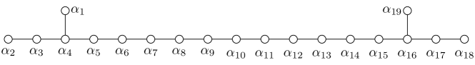
Figure 1. Coxeter diagram $G_{\rm cox}$ of $\textup{II}_{1,17}$

One has $\alpha_{i}^{2}=-2$, $\alpha_{i}\cdot\alpha_{j}=1$ if the corresponding nodes of the Coxeter diagram are connected by an edge and $0$ otherwise. Since $\textup{II}_{1,17}$ has rank $18$ there is a unique linear relation amongst the $19$ roots $\alpha_{i}$:

(4.1) $$3\alpha_{1}+2\alpha_{2}+4\alpha_{3}+\sum_{k=4}^{16}(10-k)\alpha_{k}-4\alpha_{17}-2\alpha_{18}-3\alpha_{19}=0$$

Definition 4.1.

The Coxeter fan ${\mathcal{F}}_{\rm cox}$ is defined by cutting the cone ${\overline{C}}_{\mathbb{Q}}$ by the mirrors $\alpha^{\perp}$ to the roots.

Since $W$ is a reflection group, the (orbits of) cones ${\mathcal{F}}_{\rm cox}/W$ are in a bijection with faces of $P$. The group $\Gamma$ is an extension of $W$ by $\operatorname{Aut}G_{\rm cox}={\mathbb{Z}}_{2}$. Thus, the cones in ${\mathcal{F}}_{\rm cox}/\Gamma$ are in a bijection with faces of $P$ modulo the left-right symmetry.

By [Vin75, Thm.3.3], the nonzero faces of $P$ are of two types. Type II rays corresponding to maximal parabolic subdiagrams of $G_{\rm cox}$: maximal disjoint unions of the affine Dynkin diagrams. Type III cones of dimension $18-r$ correspond to elliptic subdiagrams of $G_{\rm cox}$: disjoint unions of Dynkin diagrams with $0\leq r\leq 17$ vertices. A subset $I\subset G_{\rm cox}$ of vertices corresponds to the face $\cap_{i\in I}\alpha_{i}^{\perp}\cap P$.

The two type II rays correspond to the maximal parabolic subdiagrams ${\widetilde{E}}_{8}{\widetilde{E}}_{8}$ and ${\widetilde{D}}_{16}$. Similarly, one can count the 80 type III rays and count the higher-dimensional faces. In our special case, however, there is an easier way.

Lemma 4.2.

Suppose that an $18$-dimensional cone $P$ is defined by 19 inequalities $a_{i}\geq 0$ and that the linear forms $a_{i}$ satisfy a unique linear relation $\sum_{i=1}^{9}n_{i}a_{i}=\sum_{i=11}^{19}m_{i}a_{i}$, with $n_{i}>0$, $m_{i}>0$. Then the faces of $P$ are in a bijection with arbitrary subsets $I\subset\{1,\dotsc,19\}$ satisfying a single condition: $\{1,\dotsc,9\}\subset I$ $\iff$ $\{11,\dotsc,19\}\subset I$. A subset $I$ corresponds to the face $\cap_{i\in I}\{a_{i}=0\}\cap P$. For $I$ not containing $\{1,\dotsc,9\}$ $\operatorname{codim}F=|I|$, for those that do $\operatorname{codim}F=|I|-1$.

Proof.

A face of $P$ is obtained by intersecting $P$ with some hyperplanes $a_{i}=0$. Each point of $P$ gives a decomposition $I\sqcup I^{c}=\{1,\dotsc,19\}$ with $a_{i}=0$ for $i\in I$ and $a_{j}>0$ for $j\in I^{c}$. Obviously, $I$ must satisfy the above condition and, vice versa, for any such $I$ there exists a solution $(a_{1},\dotsc,a_{19})$. ∎

Corollary 4.3.

In ${\mathcal{F}}_{\rm cox}/W$ there are $2\cdot 9+1=19$ facets and $9^{2}+1=82$ rays. In ${\mathcal{F}}_{\rm cox}/\Gamma$ there are $9+1=10$ facets and $\frac{9\cdot 10}{2}+1=46$ rays. The total number of cones in ${\mathcal{F}}_{\rm cox}/W$ is $2N^{2}+2$ and in ${\mathcal{F}}^{\rm cox}/\Gamma$ it is $N^{2}+N+2$, where $N=2^{9}-1$.

Proof.

For ${\mathcal{F}}_{\rm cox}/W$, this follows from counting subsets $I$ satisfying the condition of Lemma 4.2. The cones in ${\mathcal{F}}_{\rm cox}/\Gamma$ biject with involution orbits of such subsets. ∎

4B. The ramification fan

Definition 4.4.

The ramification fan ${\mathcal{F}}_{\rm ram}$ is defined as a coarsening of ${\mathcal{F}}_{\rm cox}$. The unique $18$-dimensional cone is a union of four chambers $P_{\rm ram}=\cup_{g\in W_{J}}g(P)$ of ${\mathcal{F}}_{\rm cox}$, where $W_{J}={\mathbb{Z}}_{2}\oplus{\mathbb{Z}}_{2}$ is the subgroup of $W$ generated by reflections in the roots $\alpha_{1},\alpha_{19}$. The other maximal cones of ${\mathcal{F}}_{\rm ram}$ are the images $g(P_{\rm ram})$ for $g\in W$.

The corresponding toroidal compactification of $F$ is denoted ${\overline{F}}^{{\mathcal{F}}_{\rm ram}}$.

This is a special case of a generalized Coxeter semifan defined in [AET19, Sec. 10C], where its main properties are described. The data for a generalized Coxeter semifan is a subdivision $I\sqcup J$ of the nodes of $G_{\rm cox}$ into relevant and irrelevant roots. The maximal cones are the unions of the chambers $g(P)$ with $g\in W_{J}$, the subgroup generated by the reflections in the irrelevant roots, in this case $\alpha_{1},\alpha_{19}$. In general, the subgroup $W_{J}$ may be infinite and the resulting cones may not be finitely generated. In the present case the group $W_{J}$ is finite, and so ${\mathcal{F}}_{\rm ram}$ is an ordinary fan.

The cones of ${\mathcal{F}}_{\rm ram}/W$ are in a bijection with the subdiagrams of $G_{\rm cox}$ which do not have connected components consisting of the irrelevant nodes $\alpha_{1}$ and $\alpha_{19}$. The cones in ${\mathcal{F}}_{\rm ram}/\Gamma$ are in a bijection with orbits of these under $\operatorname{Aut}G_{\rm cox}={\mathbb{Z}}_{2}$. In ${\mathcal{F}}_{\rm ram}/W$ there are 17 facets and 63 rays, and in ${\mathcal{F}}_{\rm ram}/\Gamma$ 9 facets and 35 rays.

4C. The rational curve fan

Define the vectors

$$\beta_{L}=\alpha_{3}+2\alpha_{2}-\alpha_{1},\ \gamma_{L}=\alpha_{3}-\alpha_{1},\qquad\beta_{R}=\alpha_{17}+2\alpha_{18}-\alpha_{19},\ \gamma_{R}=\alpha_{17}-\alpha_{19}.$$

The fan ${\mathcal{F}}_{\rm rc}$ is a refinement of the Coxeter fan, obtained by subdividing the chamber $P$ by the hyperplanes $\beta_{L}^{\perp}$, $\gamma_{L}^{\perp}$, $\beta_{R}^{\perp}$, $\gamma_{R}^{\perp}$ into $3\cdot 3=9$ maximal-dimensional subcones $\sigma_{LR}$ with left and right ends $L,R\in\{1,2,3\}$. The other maximal-dimensional cones of ${\mathcal{F}}_{\rm rc}$ are the $W$-reflections of these cones. The involution in $\operatorname{Aut}G_{\rm cox}$ acts by exchanging $L$ and $R$. Thus, modulo $\Gamma$ there are 6 maximal cones $\sigma_{11}$, $\sigma_{12}$, $\sigma_{13}$, $\sigma_{22}$, $\sigma_{23}$, $\sigma_{33}$.

The subdivisions on the left and right sides work the same way and independently of each other. So we only explain the left side, writing simply $\beta,\gamma$ for $\beta_{L},\gamma_{L}$. Since $\gamma=\beta-2\alpha_{2}$ and $\alpha_{2}\geq 0$ on $P$, $\beta\leq 0$ implies $\gamma\leq 0$, and $\gamma\geq 0$ implies $\beta\geq 0$. Thus, the hyperplanes $\beta^{\perp}$ and $\gamma^{\perp}$ divide $P$ into three maximal cones. Fig. 2 gives a pictorial description of the subdivision and the vectors involved. One has $\beta^{2}=-8$ and $\gamma^{2}=-4$. The number of edges indicate the intersection numbers, and negative numbers are shown by dashed lines. In addition, not shown is $\beta\cdot\alpha_{1}=2$.

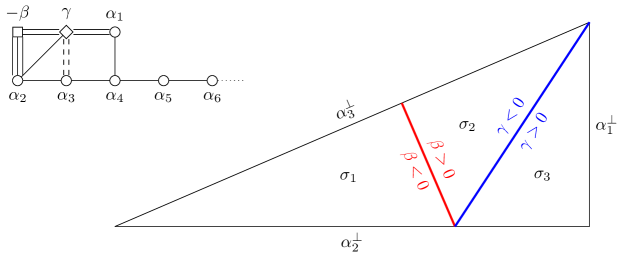
Figure 2. Subdivision of Coxeter chamber for the fan ${\mathcal{F}}_{\rm rc}$

These three maximal cones have 19 facets and the vectors defining the facets satisfy a unique linear relation:

(4.2)

$$L=1:$$

,

Here, the rest of each relation is $6\alpha_{4}+5\alpha_{5}+\dotsb$, the same as in equation (4.1) for the Coxeter chamber. Similarly, we have a subdivision into 3 cones using the hyperplanes $\beta_{R}^{\perp}$ and $\gamma^{\perp}_{R}$. Each of the resulting 9 cones $\sigma_{LR}$ has $19$ facets, with the supporting linear functions satisfying a unique linear relation. For every cone the relation has the same pattern of signs. One concludes that each of the 9 cones is ${\mathbb{Q}}$-linearly equivalent to the Coxeter chamber, and Lemma 4.2 gives a description of its faces.

For convenience define $\sigma_{L}=\cup_{R\in\{1,2,3\}}\sigma_{LR}$, which specifies only the left-end behavior. The cones $\sigma_{2}$ and $\sigma_{3}$ are related by a reflection $w$ in the $(-4)$-vector $\gamma$. Indeed, $w(\beta)=2\alpha_{2}$, $w(\alpha_{3})=\alpha_{1}$, and $w(\alpha_{i})=\alpha_{i}$ for $i\geq 4$. However, this reflection does not preserve the lattice $\textup{II}_{1,17}$. For example, $\beta$ is primitive and $2\alpha_{2}$ is 2-divisible.

There are $1+5+7+3=16$ cones of dimension $0\leq d\leq 3$ in Fig. 2. Therefore, in ${\mathcal{F}}_{\rm rc}/W$ there are $3^{2}=9$ maximal cones, $2(7+6)+1=27$ facets, $(5+6)^{2}+1=122$ rays, and a total of $2N^{2}+2$ cones, $N=16\cdot 2^{6}-1$. In ${\mathcal{F}}_{\rm rc}/\Gamma$ there are $\frac{3\cdot 4}{2}=6$ maximal cones, $7+6+1=14$ facets, $\frac{11\cdot 12}{2}+1=67$ rays, and $N^{2}+N+2$ cones.

Definition 4.5.

The toroidal compactification corresponding to the fan ${\mathcal{F}}_{\rm rc}$ is denoted ${\overline{F}}^{{\mathcal{F}}_{\rm rc}}$.

Since the fan ${\mathcal{F}}_{\rm rc}$ is very important for this paper, we describe it in more detail and give each cone a unique $ADE$ label. First, to each maximal cone $\sigma_{L}$ we associate a Coxeter diagram whose vertices correspond to the facets $v^{\perp}$ with $v\geq 0$ on $\sigma_{L}$. Then a face $F$ of $\sigma_{L}$ is described by a subdiagram of black vertices for the vectors $v$ such that $F\subset v^{\perp}$. In Table 1 we list several cones of codimension $0,1,2,3$. For a cone lying in more than one of the maximal cones $\sigma_{1},\sigma_{2},\sigma_{3}$, we can choose either of them to describe $F$, and we indicate our choice in bold in the first column.

For each cone, we also indicate which other linear functions $\alpha_{i},\beta,\gamma$ vanish on it. Namely, on the cone $\sigma_{2}\cap\sigma_{3}=\gamma^{\perp}$ one has $\alpha_{1}=\alpha_{3}$ and $\beta/2=\alpha_{2}$, so once one of them vanishes then so does the other.

Cone	Symbol	Diagram
${\bm{\sigma}_{1}}$	$E_{0}$
${\bm{\sigma}_{2}}$	$D^{\prime}_{0}$
${\bm{\sigma}_{3}}$	$D_{0}$
${\bm{\sigma}_{2}}\cap\sigma_{1}$	$E_{1}$
${\bm{\sigma}_{3}}\cap\alpha_{2}^{\perp}$	$E^{\prime}_{1}$
${\bm{\sigma}_{2}\bm{\cap}\bm{\sigma}_{3}}$	$D_{1}$
${\bm{\sigma}_{2}\bm{\cap}\bm{\sigma}_{3}}\cap\sigma_{1}$	$E_{2}$
${\bm{\sigma}_{2}\bm{\cap}\bm{\sigma}_{3}}\cap\alpha_{1}^{\perp}$	$D_{2}$
${\bm{\sigma}_{2}\bm{\cap}\bm{\sigma}_{3}}\cap\sigma_{1}\cap\alpha_{1}^{\perp}$	$E_{3}$

Table 1. Basic type III cones in ${\mathcal{F}}_{\rm rc}$

The lower-dimensional cones are obtained from these cones by intersecting with some $\alpha_{i}^{\perp}$ for $i\geq 4$. The diagram is then obtained by marking these nodes black. Adding to the $D_{2}$ and $E_{3}$ diagrams adjacent vertices makes it into larger $D_{n}$, $E_{n}$ diagrams. Marking some of the vertices that are not adjacent to the end $D$ and $E$ diagrams adds some $A_{n}$ inside the chain $\alpha_{4},\dotsc,\alpha_{16}$.

Remark 4.6.

The reason for the $ADE$ notation is as follows: Starting with $D_{2}$ and $E_{3}$, the cone is already a cone of the Coxeter fan ${\mathcal{F}}_{\rm cox}$, so we use a subdiagram of the Coxeter diagram of Fig. 1 to label it. Note that for an $E_{n}$ diagram one gets a nonzero cone only if $n\leq 9$. For $n\leq 8$ this is an elliptic subdiagram of Fig. 1, i.e. a type III cone; for $n=9$ the cone $\cap\alpha_{i}^{\perp}\cap{\overline{C}}_{\mathbb{Q}}$ is the Type II ${\widetilde{E}}_{8}{\widetilde{E}}_{8}$ ray.

We chose the labels $E_{0}$, $E_{1}$, $E^{\prime}_{1}$, $E_{2}$, $D_{0}$, $D^{\prime}_{0}$, $D_{1}$ by analogy with the larger $E$ and $D$ diagrams. This will be further explained in Section 7.

Notation 4.7.

To make the resulting $ADE$ label unique, we add the symbol $A_{0}$ to denote adjacent unmarked vertices. By a convention, explained further Section 7, we assign each label a charge: $Q(A_{n})=n+1$, $Q(D_{n})=n+4$, $Q(E_{n})=n+3$, and we require the sum of charges to be $24$. With these notations, a string of four white vertices is denoted by $A_{0}^{3}$ and adding black vertices to the interior two vertices produces diagrams $A_{1}A_{0}$, $A_{0}A_{1}$, $A_{2}$.

We summarize this discussion as follows:

Lemma 4.8.

In the fan ${\mathcal{F}}_{\rm rc}$ there are 9 maximal cones $\sigma_{ij}$, $1\leq i,j\leq 3$ modulo $W(\textup{II}_{1,17})$ with the Dynkin labels, where $(D_{0}|D_{0}^{\prime})$ denotes either $D_{0}$ or $D_{0}^{\prime}$:

$$E_{0}A_{0}^{18}E_{0},\ E_{0}A_{0}^{17}(D_{0}|D_{0}^{\prime}),\ (D_{0}|D_{0}^{\prime})A_{0}^{17}E_{0},\ (D_{0}|D_{0}^{\prime})A_{0}^{16}(D_{0}|D_{0}^{\prime}),$$

All type III cones are in a bijection with the labels

$$(E_{n_{0}}|E^{\prime}_{1}|D_{n_{0}}|D_{0}^{\prime})A_{n_{1}}\dotsc A_{n_{k}}(E_{n_{k+1}}|E^{\prime}_{1}|D_{n_{k+1}}|D_{0}^{\prime})$$

with some $n_{i}\geq 0$, and with $n_{i}\leq 8$ for the $E_{n}$ diagrams, of total charge $24$.

Next, we list the type II rays of ${\mathcal{F}}_{\rm rc}$. They are the rays of the rational closure ${\overline{C}}_{{\mathbb{Q}}}$ of the cone $\{v^{2}>0\}$, so they are the same as for the Coxeter fan. In the fan ${\mathcal{F}}_{\rm rc}$, the ${\widetilde{E}}_{8}{\widetilde{E}}_{8}$ ray is contained in each of the 9 cones $\sigma_{ij}$, and the ${\widetilde{D}}_{16}$ ray is contained in $\sigma_{ij}$ for $i=2,3$, $j=2,3$.

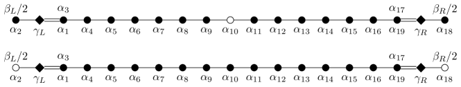
Figure 3. Type II cones in ${\mathcal{F}}_{\rm rc}$: ${\widetilde{E}}_{8}{\widetilde{E}}_{8}$ and ${\widetilde{D}}_{16}$, shown in $\sigma_{33}$

We conclude this section with a result which goes a long way towards explaining some peculiar features of the fan ${\mathcal{F}}_{\rm rc}$ which otherwise may seem quite mysterious.

Recall: Let ${\mathcal{F}}$ be a fan in a lattice $N$ defining a toric variety $X({\mathcal{F}})$. A cone $\tau\in{\mathcal{F}}$ defines a torus orbit $O(\tau)$ whose closure is $X(\tau)\subset X({\mathcal{F}})$. Denote $N_{\tau}=N\cap{\mathbb{R}}\tau$. Then $X(\tau)$ is a toric variety for the fan $\operatorname{Star}(\tau)$ in the lattice $N/N_{\tau}$.

Also recall that the root lattices $C_{n}$ and $D_{n}$ are the same but their Weyl groups are different: $W(D_{n})\subset W(C_{n})$ is a subgroup of index 2.

Lemma 4.9.

Let $\Delta=\{\alpha_{1},\alpha_{3},\alpha_{4},\alpha_{5}\dots\}$ be a $D_{n}$ subdiagram in the Coxeter graph of Fig. 1 and $\tau\in{\mathcal{F}}_{\rm cox}$ be the corresponding cone. Then $\operatorname{Star}(\tau)$ in ${\mathcal{F}}_{\rm cox}$ is the Coxeter fan for $W(D_{n})$ but $\operatorname{Star}(\tau)$ in ${\mathcal{F}}_{\rm rc}$ is the Coxeter fan for $W(C_{n})$.

Proof.

Note first that replacing either $\alpha_{1}$ or $\alpha_{3}$ by the $(-4)$-vector $\gamma=\alpha_{3}-\alpha_{1}$ transforms $\Delta$ into a $C_{n}$ Dynkin diagram. Also note that by (7.57) the $\Delta$ root sublattice of $\textup{II}_{1,17}$ is saturated.

The statement for $\operatorname{Star}(\tau)$ in ${\mathcal{F}}_{\rm cox}$ is standard. The hyperplane $\gamma^{\perp}$ divides the fundamental chamber for $W(D_{n})$ into two halves, each a fundamental chamber for $W(C_{n})$. The reflection in $\gamma$ is not defined on $N=\textup{II}_{1,17}$ but it is well defined on $N/N_{\tau}$ which is the dual of the root lattice $D_{n}$, the same as for $C_{n}$. ∎

Remark 4.10.

We will see in Section 7 that the moduli of the corresponding stable surfaces are described by $T(C_{n})/W(C_{n})$, where $T(C_{n})$ is the torus $\operatorname{Hom}(C_{n},{\mathbb{C}}^{*})$. The map $T(D_{n})/W(D_{n})\to T(C_{n})/W(C_{n})$ is $2:1$. This leads to an involution on a part of the fan ${\mathcal{F}}_{\rm rc}$ and to the two cones $D_{0}$, $D^{\prime}_{0}$ mapping to a unique stable surface of type $C_{0}$. This $D/C$ dichotomy appears to be the main reason for the refinement ${\mathcal{F}}_{\rm rc}$ of ${\mathcal{F}}_{\rm cox}$.

5. Degenerations of K3 surfaces and integral-affine spheres

To prove that ${\overline{F}}^{\rm slc}$ coincides with a toroidal compactification, we extend the method developed in [AET19]. Central to this method is the notion of an integral affine pair $(\operatorname{IAS}^{2},R_{\rm IA})$ consisting of a singular integral-affine sphere and an effective integral affine divisor on it. From a nef model of a type III one-parameter degeneration, we construct a pair $(\operatorname{IAS}^{2},R_{\rm IA})$. Vice versa, given a pair $(\operatorname{IAS}^{2},R_{\rm IA})$ we construct a combinatorial type of nef model.

Definition 5.1.

An integral-affine structure on an oriented real surface $B$ is a collection of charts to $\mathbb{R}^{2}$ whose transition functions lie in $\operatorname{SL}_{2}(\mathbb{Z})\ltimes\mathbb{R}^{2}$.

On the sphere, such structures must have singularities. We review some unpublished material from [EF18] on these singularities. Let $\widetilde{\operatorname{SL}}_{2}(\mathbb{R})\to\operatorname{SL}_{2}(\mathbb{R})$ be the universal cover. This restricts to an exact sequence

$$0\to\mathbb{Z}\to\widetilde{\operatorname{SL}}_{2}(\mathbb{Z})\to\operatorname{SL}_{2}(\mathbb{Z})\to 0.$$

Since $\operatorname{SL}_{2}(\mathbb{R})$ acts on $\mathbb{R}^{2}\setminus\{0\}$, its universal cover and the subgroup $\widetilde{\operatorname{SL}}_{2}(\mathbb{Z})$ act on $\widetilde{\mathbb{R}^{2}\setminus 0}$, which admits natural polar coordinates $(r,\theta)\in\mathbb{R}^{+}\times\mathbb{R}$. A generator of the kernel $\mathbb{Z}$ acts by the deck transformation $(r,\theta)\mapsto(r,\theta+2\pi)$.

Definition 5.2.

A naive singular integral-affine structure on $B$ is an integral-affine structure on the complement $B\backslash\{p_{1},\dots,p_{n}\}$ of a finite set such that each point $p_{i}$ has a punctured neighborhood $U_{i}\setminus\{p_{i}\}$ modeled by an integral-affine cone singularity: The result of gluing a circular sector

$$\{\theta_{1}\leq\theta\leq\theta_{2}\}\subset\widetilde{\mathbb{R}^{2}\setminus 0}$$

along its two edges $\theta=\theta_{1},\theta_{2}$ by an element of $\widetilde{\operatorname{SL}}_{2}(\mathbb{Z})$.

Definition 5.3.

Let $(B,p)$ be an integral-affine cone singularity. We may assume that $\theta_{1},\theta_{2}$ have rational slopes. Decompose $\theta_{1}\leq\theta\leq\theta_{2}$ into standard affine cones, i.e. regions $\operatorname{SL}_{2}(\mathbb{Z})$-equivalent to the positive quadrant. Let $\{\vec{e}_{1},\dots,\vec{e}_{n}\}$ denote the successive primitive integral vectors pointing along the one-dimensional rays of this decomposition. Define integers $d_{i}$ by the formula

$$\vec{e}_{i-1}+\vec{e}_{i+1}=d_{i}\vec{e}_{i}$$

using the gluing to define $d_{1}$. Then the charge is

$$Q(B,p):=12+\sum(d_{i}-3)$$

and does not depend on the choice of decomposition into standard affine cones.

By [EF18, KS06], a naive singular integral-affine structure on a compact oriented surface $B$ of genus $g$ satisfies $\sum Q(B,p_{i})=12(2-2g)$. As we are interested in the sphere, the sum of the charges of singularities is $24$. This formula was first proven by [FM83, Prop. 3.7] in the context of the dual complex of a Kulikov degeneration, see Thm. 5.16. For application to degenerations of K3 surfaces, we need a more refined notion of integral-affine singularity.

Definition 5.4.

An anticanonical pair $(Y,D)$ is a smooth rational surface $Y$ and an anticanonical cycle $D=D_{1}+\dots+D_{n}\in|-K_{Y}|$ of rational curves. Define $d_{i}:=-D_{i}^{2}$.

Definition 5.5.

The naive pseudo-fan $\mathfrak{F}(Y,D)$ of an anticanonical pair is a integral-affine cone singularity constructed as follows: For each node $D_{i}\cap D_{i+1}$ take a standard affine cone $\mathbb{R}_{\geq 0}\{\vec{e}_{i},\vec{e}_{i+1}\}$ and glue these cones by elements of $\operatorname{SL}_{2}(\mathbb{Z})$ so that $\vec{e}_{i-1}+\vec{e}_{i+1}=d_{i}\vec{e}_{i}$.

Remark 5.6.

Note that the cone singularity itself does not keep track of the rays. For instance, blowing up the node $D_{i}\cap D_{i+1}$ produces a new anticanonical pair $(Y^{\prime},D^{\prime})\to(Y,D)$ whose naive pseudo-fan $\mathfrak{F}(Y^{\prime},D^{\prime})$ is identified with $\mathfrak{F}(Y,D)$. The standard affine cone $\mathbb{R}_{\geq 0}\{\vec{e}_{i},\vec{e}_{i+1}\}$ is subdivided in two. The charge $Q(Y,D):=Q(\mathfrak{F}(Y,D))$ is invariant under such a corner blow-up.

Definition 5.7.

The c.b.e.c. (corner blow-up equivalence class) of $(Y,D)$ is the equivalence class of anticanonical pairs which can be reached from $(Y,D)$ by corner blow-ups and blow-downs.

Remark 5.6 implies that $\mathfrak{F}(Y,D)$ depends only on the c.b.e.c. of $(Y,D)$.

Definition 5.8.

A toric model of a c.b.e.c. is a choice of representative $(Y,D)$ and an exceptional collection: A sequence of $Q(Y,D)$ successively contractible $(-1)$-curves which are not components of $D$. The blowdown $(\overline{Y},\overline{D})$ is a toric pair, i.e. a toric surface with its toric boundary. We call these internal blow-ups.

Definition 5.9.

An integral-affine singularity is an integral-affine cone singularity isomorphic to $\mathfrak{F}(Y,D)$ for some anticanonical pair $(Y,D)$, with a multiset of rays $\{\vec{e}_{i}\}$ corresponding to the components $D_{i}\subset D$ meeting an exceptional collection. The pseudo-fan $\mathfrak{F}(Y,D)$ is the naive pseudo-fan, equipped with this data.

Note that the components $D_{i}\subset D$ meeting an exceptional collection uniquely determine the deformation type of the anticanonical pair $(Y,D)$.

Definition 5.10.

Let $\phi\colon\mathfrak{F}(Y,D)\rightarrow\mathfrak{F}(Y^{\prime},D^{\prime})$ be an isomorphism of integral-affine cone singularities. We say that $\phi$ is an isomorphism of integral-affine singularities if the two multisets of rays $\{\phi(\vec{e}_{i})\}$ and $\{\vec{e}_{i}^{\prime}\}$ determine the same deformation type.

Equivalently, after making corner blow-ups on $(Y^{\prime},D^{\prime})$ until the rays $\phi(\vec{e}_{i})$ all form edges of the decomposition of $\mathfrak{F}(Y^{\prime},D^{\prime})$ into standard affine cones, the pair $(Y^{\prime},D^{\prime})$ admits an exceptional collection meeting the components corresponding to $\phi(\vec{e}_{i})$. From the definitions, integral-affine singularities, up to isomorphism, are in bijection with c.b.e.c.s of deformation types of anticanonical pairs $(Y,D)$. We are now equipped to remove the word “naive” in Definition 5.2.

Definition 5.11.

An integral-affine sphere, or $\operatorname{IAS}^{2}$ for short, is an integral-affine structure on the sphere with integral-affine singularities as in Definition 5.9.

In particular, there is a forgetful map from $\operatorname{IAS}^{2}$ to naive $\operatorname{IAS}^{2}$ which forgets the data of the multisets of outgoing rays from each singularity.

Definition 5.12.

Let $(\vec{v}_{1},\dots,\vec{v}_{k})$ be a counterclockwise-ordered sequence of primitive integral vectors in $\mathbb{R}^{2}$ and let $n_{i}$ be positive integers. We define an integral-affine singularity $(B,p)=I(n_{1}\vec{v}_{1},\dots,n_{k}\vec{v}_{k})$ by declaring $(B,p)=\mathfrak{F}(Y,D)$ where $(Y,D)$ is a blow-up of a smooth toric surface $(\overline{Y},\overline{D})$ whose fan contains the rays $\mathbb{R}_{\geq 0}\vec{v}_{i}$ at $n_{i}$ points on the component $\overline{D}_{i}$ corresponding to $\vec{v}_{i}$.

Every c.b.e.c. admits some toric model and hence can be presented in the form $I(n_{1}\vec{v}_{1},\dots,n_{k}\vec{v}_{k})$. Since $Q(I(n_{1}\vec{v}_{1},\dots,n_{k}\vec{v}_{k}))=\sum n_{i}\geq 0$, an integral-affine surface with singularities, as defined, is either a non-singular $2$-torus, or the $2$-sphere.

Definition 5.13.

Define the $I_{k}$ singularity as $I(k\vec{e})$. It has charge $k$.

Remark 5.14.

If an $\operatorname{IAS}^{2}$ has all $I_{1}$ singularities there are $24$ such. There is only one integral-affine singularity which underlies the naive cone singularity of $I(\vec{e})$, corresponding to either marking the ray $\vec{e}$ or $-\vec{e}$. Hence in the case where all $24$ charges are distinct, there is no difference between a naive $\operatorname{IAS}^{2}$ and an $\operatorname{IAS}^{2}$.

Definition 5.15.

An $\operatorname{IAS}^{2}$ is generic if it has $24$ distinct $I_{1}$ singularities.

The relevance of these definitions lies in the following:

Theorem 5.16.

Let $X\rightarrow C$ be a Type III Kulikov model. The dual complex $\Gamma(X_{0})$ has the structure of an $\operatorname{IAS}^{2}$, triangulated into lattice triangles of lattice volume 1. Conversely, such a triangulated $\operatorname{IAS}^{2}$ with singularities at vertices determines a Type III central fiber $X_{0}$ uniquely up to topologically trivial deformations.

Proof.

See [Eng18] or [GHK15a, Rem1.11v1] for the forward direction. Roughly, one glues together unit volume lattice triangles by integral-affine maps, in such a way that the vertex $v_{i}$ corresponding to a component $V_{i}\subset X_{0}$ has integral-affine singularity $\mathfrak{F}(V_{i},D_{i})$. Here $D_{i}=\sum_{j}D_{ij}$ and $D_{ij}:=V_{i}\cap V_{j}$ are the double curves lying on $V_{i}$. For the reverse direction, one glues together the anticanonical pairs $(V_{i},D_{i})$ whose pseudo-fans model the vertices of the triangulated $\operatorname{IAS}^{2}$. The gluings are ambiguous, but all such gluings give homeomorphic surfaces $X_{0}$ which are related by topologically trivial deformations. ∎

Definition 5.17.

Let $B$ be an $\operatorname{IAS}^{2}$. An integral-affine divisor $R_{\rm IA}$ on $B$ consists of two pieces of data:

1. A weighted graph $R_{\rm IA}\subset B$ with vertices $v_{i}$, rational slope line segments as edges $v_{ij}$, and integer labels $n_{ij}$ on each edge.

2. Let $v_{i}\in R$ be a vertex and $(V_{i},D_{i})$ be an anticanonical pair such that $\mathfrak{F}(V_{i},D_{i})$ models $v_{i}$ and contains all edges of $v_{ij}$ coming into $v_{i}$. We require the data of a line bundle $L_{i}\in\textrm{Pic}(V_{i})$ such that $\deg{L_{i}}\big{|}_{D_{ij}}=n_{ij}$ for the components $D_{ij}$ of $D_{i}$ corresponding to edges $v_{ij}$ and $L_{i}$ has degree zero on all other components of $D_{i}$.

Definition 5.18.

A divisor $R_{{\rm IA}}\subset B$ is polarizing if each line bundle $L_{i}$ is nef and at least one $L_{i}$ is big. The self-intersection is $R_{\rm IA}^{2}:=\sum_{i}L_{i}^{2}\in\mathbb{Z}_{>0}.$

Definition 5.19.

Given an nef model $L\rightarrow X$, we get an integral-affine divisor $R_{\rm IA}\subset B=\Gamma(X_{0})$ by simply restricting $L$ to each component. Since $L$ is nef, the divisor $R_{\rm IA}$ is effective i.e. $n_{ij}\geq 0$.

Remark 5.20.

When $v_{i}\in R_{\rm IA}$ is non-singular, the pair $(V_{i},D_{i})$ is toric, and the labels $n_{ij}$ uniquely determine $L_{i}$. They must satisfy a balancing condition. If $\vec{e}_{ij}$ are the primitive integral vectors in the directions $v_{ij}$ then one must have $\sum n_{ij}\vec{e}_{ij}=0$ for such a line bundle $L_{i}$ to exist.

Similarly, if $I_{1}=\mathfrak{F}(V_{i},D_{i})=I(\vec{e})$ i.e. $(V_{i},D_{i})$ is a single internal blow-up of a toric pair, the $n_{ij}$ determine a unique line bundle $L_{i}$ so long as $\sum n_{ij}\vec{e}_{ij}\in\mathbb{Z}\vec{e}$. This condition is well-defined: the $\vec{e}_{ij}$ are well-defined up to shears in the $\vec{e}$ direction.

Let $B$ be a lattice triangulated $\operatorname{IAS}^{2}$ or equivalently, $B=\Gamma(X_{0})$ is the dual complex of a Type III degeneration. When $B$ is generic, an integral-affine divisor $R_{\rm IA}\subset B$ is uniquely specified by a weighted graph satisfying the balancing conditions of Remark 5.20, so the extra data (2) of Definition 5.17 is unnecessary.

Definition 5.21.

An integral-affine divisor $R_{\rm IA}\subset B$ is compatible with a triangulation if every edge of $R_{\rm IA}$ is formed from edges of the triangulation.

If $B$ comes with a triangulation, we assume that an integral-affine divisor is compatible with it.

6. Compactification for the ramification divisor

Theorem 6.1.

The normalization of the stable pair compactification ${\overline{F}}^{{\rm ram}}$ is the toroidal compactification ${\overline{F}}^{{\mathcal{F}}_{\rm ram}}$.

Proof.

Let $\textup{II}_{3,19}\ni h$ be the K3 lattice and a vector with $h^{2}=2$. Denote by $N_{2}$ the lattice $h^{\perp}=\textup{II}_{1,1}\oplus\textup{II}_{1,17}\oplus\langle-2\rangle$. of signature $(2,19)$ and by ${\mathbb{D}}_{2}$ be the corresponding Type IV domain. It is well known that the moduli space of polarized K3 surfaces $(X,L)$ of degree $2$ with $ADE$ singularities is the arithmetic quotient $F_{2}=O^{*}(N_{2})\backslash{\mathbb{D}}_{2}$ for a finite subgroup $O^{*}(N_{2})\subset O(N_{2})$.

There are two $O^{*}(N_{2})$-orbits of vectors $v\in N_{2}$ with $v^{2}=-2$, with representatives $v_{1}$ and $v_{2}$ of divisibility $1$, resp. $2$ in $N_{2}^{*}$. They define two hyperplanes $v_{k}^{\perp}$ in ${\mathbb{D}}_{2}$ and two Heegner divisors in $F_{2}$, for the nodal and unigonal K3 surfaces. The second hyperplane ${\mathbb{D}}=v_{2}^{\perp}$ is the Type IV domain for the lattice $N_{\operatorname{ell}}=\textup{II}_{2,18}\subset N_{2}$, and its arithmetic quotient is our space $F=F_{\operatorname{ell}}$.

There are single orbits of primitive square $0$ vectors in $N_{2}$ and in $N_{\operatorname{ell}}$. Let us a choose a representative $e\in N_{\operatorname{ell}}\subset N_{2}$. Baily-Borel compactifications ${\overline{F}}_{2}^{\rm BB}$ and ${\overline{F}}_{\operatorname{ell}}^{\rm BB}$ both have a single $0$-cusp. A toroidal compactification of $F_{2}$, resp. $F_{\operatorname{ell}}$, is described by a single fan supported on the light cone ${\overline{C}}_{\mathbb{Q}}$ for the lattice $e^{\perp}/e$, where $e^{\perp}$ is taken in $N_{2}$, resp. $N_{\operatorname{ell}}$. One has $e^{\perp}/e=\textup{II}_{1,17}\oplus\langle-2\rangle$, resp. $e^{\perp}/e=\textup{II}_{1,17}$. In particular, the Coxeter fans ${\mathcal{F}}^{2}_{\rm cox}$, resp. ${\mathcal{F}}_{\rm cox}={\mathcal{F}}^{\operatorname{ell}}_{\rm cox}$, is defined by intersecting ${\overline{C}}_{\mathbb{Q}}$ by the hyperplanes $\alpha^{\perp}$ orthogonal to the roots in $e^{\perp}/e$. It follows that the toroidal compactification ${\overline{F}}_{\operatorname{ell}}^{{\mathcal{F}}^{\operatorname{ell}}_{\rm cox}}$ is the closure of $F_{\operatorname{ell}}$ in the toroidal compactification ${\overline{F}}_{2}^{{\mathcal{F}}^{2}_{\rm cox}}$.

The fundamental domain in ${\mathcal{F}}^{2}_{\rm cox}$ is described by the Coxeter diagram with 24 vertices (fundamental roots) $\alpha_{i}$ pictured in [AET19, Fig. 4.1]. The roots of divisibility $2$ are $\alpha_{21},\alpha_{22},\alpha_{23}$. Let us take $v_{2}=\alpha_{23}$. Then the hyperplane $\alpha_{j}^{\perp}$ intersects $v_{2}^{\perp}$ iff $|\alpha_{23}\cdot\alpha_{i}|\leq 2$. Thus, the Coxeter diagram for $N_{\operatorname{ell}}$ is obtained from that for $N_{2}$ by removing the nodes $\alpha_{21},\alpha_{22},\alpha_{3}$, and the result is precisely the Coxeter diagram of Fig. 1 for lattice $\textup{II}_{1,17}$.

It is shown in [AET19] that the normalization of the stable pair compactification ${\overline{F}}_{2}^{\rm ram}$ for the ramification divisor is a semitoric compactification for the semifan ${\mathcal{F}}^{2}_{\rm ram}$ that is the coarsening of the Coxeter fan ${\mathcal{F}}^{2}_{\rm cox}$ obtained by reflecting the fundamental domain by the Weyl group $W_{2}$ generated by reflections in the six “irrelevant” roots $\alpha_{18},\dotsc,\alpha_{23}$. This group is infinite, and so ${\mathcal{F}}^{2}_{\rm ram}$ is a semifan and not a fan; the maximal-dimensional cones are not finitely generated.

It follows that ${\overline{F}}_{\operatorname{ell}}^{\rm ram}$ is the closure of $F_{\operatorname{ell}}$ in ${\overline{F}}_{2}^{\rm ram}$ and its normalization is the semitoric compactification for the fan ${\mathcal{F}}^{\operatorname{ell}}_{\rm ram}={\mathcal{F}}^{2}_{\rm ram}\cap v_{2}^{\perp}$. Thus, it is the semifan obtained by reflecting the fundamental domain of ${\mathcal{F}}^{\operatorname{ell}}_{\rm cox}$ by the Weyl group $W_{\operatorname{ell}}$ generated by reflections in “irrelevant” roots $\alpha_{18},\dotsc,\alpha_{23}$ that are not $\alpha_{21},\alpha_{22},\alpha_{3}$ and $\alpha_{23}=v_{2}$ itself. In Fig. 1 these are the two roots denoted $\alpha_{1}$ and $\alpha_{19}$. Since the two vertices 1 and 19 are disjoint, one has $W_{\operatorname{ell}}={\mathbb{Z}}_{2}\oplus{\mathbb{Z}}_{2}$, the semifan ${\mathcal{F}}^{\operatorname{ell}}_{\rm ram}$ is in fact a fan, and the semitoric compactification ${\overline{F}}_{\operatorname{ell}}^{{\mathcal{F}}_{\rm ram}}$ is toroidal. ∎

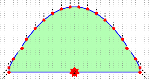
Figure 4. $(\operatorname{IAS}^{2},R_{\rm IA})$ for the ramification polarization divisor

Remark 6.2.

In [AET19] the degenerations of degree 2 K3 pairs $(X,\epsilon R)$ are described by the integral-affine pairs $(\operatorname{IAS}^{2},R_{\rm IA})$ of [AET19, Fig.9.1]. Following the proof of the above theorem, the pairs for ${\overline{F}}^{\rm ram}$ are obtained by setting $a_{23}=0$, i.e. closing the gap in the second presentation of loc. cit. We give the result in Fig. 4. The picture shows the upper hemisphere, and the entire sphere is glued from two copies like a taco or a pelmeni (a dumpling). The polarizing divisor is the equator; it is drawn in blue.

The divisor models and stable models can be read off from the pair $(\operatorname{IAS}^{2},R_{\rm IA})$: The divisor $R$ is the fixed locus of an involution on the Kulikov model which acts on the dual complex by switching the two hemispheres. Irreducible components of the stable model correspond to the vertices of $R_{\rm IA}$. Fig. 4 gives a stable model with the maximal possible number 18 of irreducible components.

7. Compactification for the rational curve divisor

7A. Kulikov models of type III degenerations

Let $L,R\in\{1,2,3\}$. Consider the following $19$ vectors in $(\frac{1}{2}\mathbb{Z})^{2}$

$$\vec{v}_{1} =\left\{\begin{array}[]{ll}(0,1)&\mbox{if }L=2,3\\ (1,\tfrac{9}{2})&\mbox{if }L=1\end{array}\right.$$

$$\vec{v}_{i} =(1,\tfrac{10-i}{2})\textrm{ if }i=2,\dots,18$$

$$\vec{v}_{19} =\left\{\begin{array}[]{ll}(0,-1)&\mbox{if }R=2,3\\ (1,-\tfrac{9}{2})&\mbox{if }R=1.\end{array}\right.$$

Let $\ell=(\ell_{1},\dots,\ell_{19})\in\mathbb{Z}_{\geq 0}^{19}$ be non-negative integers, satisfying the condition that $\sum\ell_{i}\vec{v}_{i}$ is a horizontal vector.

Form a polygon $P_{LR}(\ell)$ whose edges are the vectors $\ell_{i}\vec{v}_{i}$ put end-to-end in the plane, together with a segment on the $x$-axis. For instance $P_{1,2}(2,\dots,2,9)$ is shown in Fig. 5. Let $Q_{LR}(\ell)$ be the lattice polygon which results from taking the union of $P_{LR}(\ell)$ with its reflection across the $x$-axis.

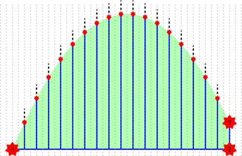
Figure 5. $(\operatorname{IAS}^{2},R_{\rm IA})$ for the rational curve polarization divisor. End behaviors: $L=1$, $R=2$ or $3$.

Definition 7.1.

Define $B_{LR}(\ell)$, a naive singular $\operatorname{IAS}^{2}$, as follows: Glue each edge $\ell_{i}\vec{v}_{i}$ of $Q_{LR}(\ell)$ to its reflected edge by an element of $\operatorname{SL}_{2}(\mathbb{Z})\ltimes\mathbb{R}^{2}$ which preserves vertical lines. This uniquely specifies the gluings, except when $\ell_{1},\ell_{19}>0$ and $L,R\in\{2,3\}$ respectively. For these edges, we must specify the gluing to be $-A^{4}$ where $A(x,y)=(x+y,y)$ is a unit vertical shear.

Remark 7.2.

As naive $\operatorname{IAS}^{2}$, we have that $B_{LR}(\ell)$ are isomorphic when we interchange the end behaviors $2\leftrightarrow 3$. It is only when we impose the extra data as in Definition 5.9 that we can distinguish them.

From Definition 7.1, we determine the $\operatorname{SL}_{2}(\mathbb{Z})$-monodromy of the naive $\operatorname{IAS}^{2}$. Assume for convenience that all $\ell_{i}>0$. Let $g_{i}\in\pi_{1}(B_{LR}(\ell)\setminus\{p_{i}\},\,*)$ for $i=1,\dots,20$ be simple counterclockwise loops based at a point $*$ in the interior of $Q_{LR}(\ell)$, which successively enclose the singularities of $B_{LR}(\ell)$ from left to right. Then the $\operatorname{SL}_{2}(\mathbb{Z})$-monodromies are:

$$\rho(g_{1}) =A^{9}\textrm{ if }L=1,\hskip 10.0pt\rho(g_{1})=\rho(g_{2})=-A^{4}\textrm{ if }L=2,3$$

$$\rho(g_{20}) =A^{9}\textrm{ if }R=1,\hskip 10.0pt\rho(g_{19})=\rho(g_{20})=-A^{4}\textrm{ if }R=2,3$$

$$\rho(g_{i}) =A^{-1}\textrm{ for all remaining }i.$$

When some $\ell_{i}=0$, the monodromy of the resulting cone singularity is the product.

Remark 7.3.

The image of the $\operatorname{SL}_{2}(\mathbb{Z})$-monodromy representation of $B_{LR}(\ell)$ lands in the abelian group $\pm A^{\mathbb{Z}}$. This is related to the existence of a broken elliptic fibration on the corresponding Kulikov models. When all $24$ singularities are distinct, the monodromy of an $\operatorname{IAS}^{2}$ is never abelian, because the sphere would then admit a non-vanishing vector field. Here, we always have some singularity of charge $\geq 2$.

Next, we enhance $B_{LR}(\ell)$ from a naive $\operatorname{IAS}^{2}$ to an $\operatorname{IAS}^{2}$:

Definition 7.4.

The multisets of rays (cf. Definition 5.9) giving toric models of the anticanonical pairs whose pseudo-fans model each singularity are listed in Table 3. The rays are chosen with respect to the open chart $Q_{LR}(\ell)$ on $B_{LR}(\ell)$. The marked rays for right end $R$ are analogous, but reflected across the $y$-axis.

Table 2. Pseudofans modeling each singularity, for the left end type $L$

$L$	Singularity	Marked rays	Notation
$1$	$\ell_{1}\neq 0$, end singularity	$(1,-3),(1,0),(1,3)$	$X_{3}$
$1,2$	$\ell_{1}=0$, $\ell_{2}\neq 0$	$(1,-2),(1,0),(1,1),(1,3)$	$X_{4}$
$3$	$\ell_{1}=0$, $\ell_{2}\neq 0$	$(1,-2),(1,0),(1,2),(1,4)$	$X^{\prime}_{4}$
$1,2,3$	$\ell_{i}=0$ for $i\leq k$, $k\geq 2$	All choices equivalent	$X_{k+3}$
$2,3$	$\ell_{1}\neq 0$, inner singularity	$(1,0),(1,2)$	$Y_{2}$
$2$	$\ell_{1},\ell_{2}\neq 0$, outer singularity	$(1,1),(1,3)$	$Y_{2}$
$3$	$\ell_{1},\ell_{2}\neq 0$, outer singularity	$(1,2),(1,4)$	$Y^{\prime}_{2}$
$2,3$	$\ell_{1}\neq 0,\,\ell_{i}=0$ for $2\leq i\leq k$	All choices equivalent	$Y_{k+1}$
	$\ell_{i+j}=0$, $1\leq j\leq k$ in interior	$(0,-1)$, multiplicity $k$	$I_{k}$

Table 3. All allowable combinatorial types of $\operatorname{IAS}^{2}$

	$L$ Symbol(s)	Intermediate Symbols	$R$ Symbol(s)
$L=1$	$X_{3}$	$I_{1+n_{1}}\cdots I_{1+n_{k}}$, $n_{i}\geq 0$	$X_{3}$	$R=1$
$L=2$	$Y_{2}Y_{2}$		$Y_{2}Y_{2}$	$R=2$
$L=3$	$Y_{2}Y_{2}^{\prime}$ or $X_{4}^{\prime}$		$Y_{2}^{\prime}Y_{2}$ or $X_{4}^{\prime}$	$R=3$
$L=1,2$	$X_{4}$		$X_{4}$	$R=1,2$
$L=2,3$	$Y_{2}Y_{2+n}$, $n\geq 1$		$Y_{2}Y_{2+n}$, $n\geq 1$	$R=2,3$
$L=1,2,3$	$X_{3+n}$, $n\geq 2$		$X_{3+n}$, $n\geq 2$	$R=1,2,3$

When an end is an isolated point, the symbol $X$ is used. When the left end is a vertical segment the symbols $Y$ are used for the so-called inner and outer singularities at the points $p_{1}$ and $p_{2}$, respectively. The same applies to $p_{20}$ and $p_{19}$ at the right end. For instance, in Fig. 5, there is one left-most singularity, labeled $X_{3}$. There are two right-most singularities. Both are labeled $Y_{2}$ and the upper right-most singularity in the figure is the “outer singularity.” The lower right-most singularity is the “inner singularity.” Intermediate singularities are labeled $I_{k}$ and in Fig. 5, specifically $I_{1}$.

The singularities notated $Y_{2}$ and $Y^{\prime}_{2}$ are abstractly isomorphic, but the prime is necessary to distinguish how the marked rays sit on the sphere $B_{LR}(\ell)$ at the outer singularity. This is distinguishes Ends $2$ and $3$, respectively.

Notation 7.5.

Table 3 allows for very succinct notation for the types of $\operatorname{IAS}^{2}$ that appear in our construction. For instance, if $(L,R)=(3,2)$ and $\ell_{i}\neq 0$ for exactly $i=2,5,6,16,19$ then we say that $B_{LR}(\ell)$ is of combinatorial type $X^{\prime}_{4}I_{3}I_{1}I_{10}Y_{4}Y_{2}$ indicating the sequence of singularities one sees traveling along the vectors $\ell_{i}\vec{v}_{i}$. The subscripts denote the charges, so they always add to $24$. As another example, Fig. 5 has an $\operatorname{IAS}^{2}$ of combinatorial type $X_{3}I_{1}^{17}Y_{2}Y_{2}$ assuming that $R=2$. If $R=3$, the combinatorial type is instead $X_{3}I_{1}^{17}Y_{2}^{\prime}Y_{2}$. Generally, all allowable combinatorial types can be formed by concatenating symbols as in Table 3 in an arbitrary manner, choosing one symbol out of each column, in such a way that the sum of all indices is $24$, and ensuring that no $X$-symbol has an index of $12$ or more.

Lemma 7.6.

The types of the $\operatorname{IAS}^{2}$ defined above are in a bijection with the types III cones in the fan ${\mathcal{F}}_{\rm rc}$ of Lemma 4.8 via the correspondence of symbols $E_{n}=X_{n+3}$, $E^{\prime}_{1}=X^{\prime}_{4}$, $D_{n}=Y_{2}Y_{2+n}$, $D^{\prime}_{0}=Y_{2}Y^{\prime}_{2}$, and $A_{n}=I_{n+1}$.

Proof.

We have defined 9 maximal dimensional cones in $\mathcal{F}_{\rm rc}$ modulo $W$ and 9 types of $\operatorname{IAS}^{2}$, with the Dynkin labels $(E_{0}|D_{0}|D^{\prime}_{0})A_{0}^{18|17|16}(E_{0}|D_{0}|D^{\prime}_{0})$ and with combinatorial types $(X_{3}|Y_{2}Y_{2}|Y_{2}Y_{2}^{\prime})I_{I}^{18|17|16}(X_{3}|Y_{2}Y_{2}|Y_{2}^{\prime}Y_{2})$, respectively. For each type, an $\operatorname{IAS}^{2}$ is defined by the collection of positive numbers $\ell_{i}$ satisfying a single linear relation, that the height difference from the left end to the right end is zero. This linear relation between the $\ell_{i}$ has 9 positive coefficients, 1 zero coefficient, and 9 negative coefficients.

On the other hand, a point $\lambda$ in a maximal cone is defined by a collection of 19 nonnegative numbers, the intersection numbers between $\lambda$ and the 19 vectors among $\alpha_{i}$, $\beta_{L}$, $\gamma_{L}$, $\beta_{R}$, $\gamma_{R}$ that give the facets of this cone. These intersection numbers satisfy the relations given in equation (4.2) with the same sign pattern. In fact, one checks that the formulas given in Cor. 7.33 give an explicit bijection between lattice points in the interiors of the 9 maximal cones of $\mathcal{F}_{\rm rc}$ and $\operatorname{IAS}^{2}$ of the corresponding combinatorial type with all $\ell_{i}>0$. This bijection extends to the faces the maximal cones, by allowing some $\ell_{i}=0$, and giving the symbol substitution rules described in the lemma. ∎

We now decompose $B_{LR}(\ell)$ into unit width vertical strips (in fact these are integral-affine cylinders). Cut these cylinders by the horizontal line along the base of $P_{LR}(\ell)$ joining the left to the right end, to form a collection of unit width trapezoids, and triangulate each trapezoid completely into unit lattice triangles.

Remark 7.7.

If $\ell_{i}$ is odd for some odd $i$, the singularities of $B_{LR}(\ell)$ may not lie at integral points. In these cases, we can adjust the location of the singularity by moving it vertically half a unit. This destroys the involution symmetry of $B_{LR}(\ell)$, but the singularities of $B_{LR}(\ell)$ will be vertices of the triangulation. Alternatively, we could just triangulate $B_{LR}(2\ell)$ in the same manner, but our current approach allows for a wider range of valid $\ell$ values.

Definition 7.8.

Define $X_{0,LR}(\ell)$ to be the unique deformation type of Type III Kulikov surface associated to the triangulated $B_{LR}(\ell)$ by Theorem 5.16.

Shifting singularities and replacing $\ell\mapsto 2\ell$ as in Remark 7.7 has the effect [EF21, Sec. 4] of birational modifications and an order $2$ base change to the Kulikov model in Definition 7.8, neither of which ultimately affect the stable model.

Example 7.9.

The deformation type of an anticanonical pair $(V,D)$ forming a component of $X_{0,LR}(\ell)$ can be quickly read off from Table 3. For instance, the singularity $X^{\prime}_{4}$ is the result of gluing the circular sector $\mathbb{R}_{\geq 0}\{(1,-4),(1,4)\}$ by $A^{8}(x,y)=(x,8x+y)$ and has the rays $(1,-2),(1,0),(1,2),(1,4)$ marked. To realize this singularity as a pseudo-fan we should further decompose the circular sector into standard affine cones so that the one-dimensional rays are $\vec{e}_{n}=(1,n)$ for $n=-4,\dots,4$. By the formula $\vec{e}_{i-1}+\vec{e}_{i+1}=-D_{i}^{2}\vec{e}_{i}$ we have that the anticanonical cycle of $(Y,D)$ consists of eight $(-2)$-curves—computing $-D_{4}^{2}$ requires taking indices mod $8$ and performing the gluing.

The marked rays indicate that four disjoint exceptional curves meet $D_{-2}$, $D_{0}$, $D_{2}$, $D_{4}$. Blowing these down gives the unique toric surface whose anticanonical cycle has self-intersections $(-1,-2,-1,-2,-1,-2,-1,-2)$, which is itself the blow-up of $\mathbb{P}^{1}\times\mathbb{P}^{1}$ at the four corners of an anticanonical square.

7B. Nef and divisor models of degenerations

We assume henceforth that our polarizing divisor is $R=s+\sum f_{i}$. The case $R=s+m\sum f_{i}$ is treated similarly, by simply adding factors of $m$ to anything vertical.

Define a polarizing divisor $R_{{\rm IA}}$ on every $\operatorname{IAS}^{2}$ of the form $B_{LR}(\ell)$ as follows: The underlying weighted graph of $R_{{\rm IA}}$ is the union of the following straight lines:

1. the horizontal line joining the two ends, with label $n_{ij}=1$, and

2. the vertical line through any singularity, with label $n_{ij}=Q$, where $Q$ is the total charge of the singularities on the vertical line.

See Figure 5, where the graph is shown in blue (note that a copy is reflected across the $x$-axis). In the example, the label of the right-hand vertical blue segment is $4$.

To give a complete definition of $R_{{\rm IA}}$ as in Definition 5.17 requires choosing various line bundles. It is simpler to directly specify the divisor model by giving a divisor $R_{i}$ on each component of $V_{i}\subset\mathcal{X}_{0,LR}(\ell)$ with appropriate intersection numbers with the double curves, i.e. $R_{i}\cdot D_{ij}=n_{ij}$. These are listed in Table 4 and require some explanation.

${X_{k+3}\,(k\geq 0)}$, ${X^{\prime}_{4}:}$ The end component $(V,D)$ is an anticanonical pair with $D$ a cycle of $(-2)$-curves of length $9-k$. Thus, $(V,D)$ is in the deformation type of an elliptic rational surface with $D$ a fiber of Kodaira type $I_{9-k}$. We assume that $(V,D)$ is in fact elliptic. The $f_{i}$ in Table 4 are the $Q(V,D)=k+3$ singular elliptic fibers not equal to $D$ and $s$ is a section. When $Q=4$, the two cases $X_{4}$ and $X^{\prime}_{4}$ are the two different deformation types of pairs $(V,D)$ with a cycle of eight $(-2)$-curves. In the $X^{\prime}_{4}$ case, $\oplus\mathbb{Z}D_{i}$ is an imprimitive sublattice of $H^{2}(Y,\mathbb{Z})$; in the $X_{4}$ case it is a primitive sublattice.

Inner ${Y_{2}}$: Taking $(1,0),(0,1)$ to be the rays of the pseudo-fan with polarization degrees $1$ and $Q$ respectively, we get a pair $(\mathbb{F}_{1},D_{1}+D_{2})$ with $D_{1}^{2}=0$ and $D_{2}^{2}=4$. Note $D_{2}$ is a bisection of the ruling on $\mathbb{F}_{1}$ with fiber class $D_{1}$. Then $s$ is the $(-1)$-section and $f_{1}$ and $f_{2}$ are the two fibers in the class of $D_{1}$ tangent to the bisection $D_{2}$. The fibers $f_{i}^{\prime}$ are $Q-4$ other fibers in the same class as, but not equal to $D_{1}$. Here $Q$ is the total charge at the end.

Outer ${Y_{2}}$ and ${Y^{\prime}_{2}}$: Taking $(0,-1),(1,4)$ to be the rays of the pseudo-fan with polarization degrees $4$ and $0$ respectively, we get $Y_{2}=\mathfrak{F}(\mathbb{F}_{1},D_{1}+D_{2})$ and $Y^{\prime}_{2}=\mathfrak{F}(\mathbb{F}_{0},D_{1}+D_{2})$ with $D_{1}^{2}=4$ and $D_{2}^{2}=0$ in both cases. Then $f_{1}$ and $f_{2}$ are the two fibers in the class of $D_{2}$ tangent to the bisection $D_{1}$. Our notation with the prime indicates that $Y_{2}$ represents the “primitive” case, and $Y^{\prime}_{2}$ the “imprimitive” case.

${Y_{k+2}\,(k\geq 0):}$ Take $(0,-1),(1,4-k)$ to be the rays of the pseudo-fan. This anticanonical pair $(V,D_{1}+D_{2})$ has self-intersections $D_{1}^{2}=4-k$ and $D_{2}^{2}=0$ respectively. It is the result of blowing up either of the previous two cases at $k$ points on $D_{1}$. These cases coincide once $k>0$. Then $f_{1}$ and $f_{2}$ are the pullbacks of the original two fibers tangent to the bisection, and the $f_{i}^{\prime}$ are pullbacks of fibers which go through the points blown up on $D_{1}$.

${I_{k}:}$ Take $(0,-1),(0,1)$ and two rays pointing left and right to be the rays of the pseudo-fan. Then $(V,D)$ is the blow-up of some Hirzebruch surface $\mathbb{F}$ at $k$ points on a section. The $f_{i}$ are the pullbacks of fibers going through blown up points.

Non-singular surfaces: All non-singular surfaces $V_{i}$ are toric and ruled over either of the double curves corresponding to the vertical direction. The $f_{i}$ are fibers of this ruling. The total count of fibers is $Q$ where $Q$ is the total charge on the vertical line through the vertex $v_{i}\in B_{LR}(\ell)$. At intersection points where the horizontal and vertical lines of $R_{IA}$ meet, we include a section of the vertical fibration. At an end of type $2$ or $3$, two of the fibers $f_{1}$ and $f_{2}$ are quadrupled.

Table 4. Divisors on each anticanonical pair

Singularity	$R_{i}\subset V_{i}\subset X_{0,LR}(\ell)$
$X_{k+3}$, $X^{\prime}_{4}$	$s+\sum_{i=1}^{k+3}f_{i}$
inner $Y_{2}$	$s+2f_{1}+2f_{2}+\sum_{i=1}^{Q-4}f_{i}^{\prime}$
outer $Y_{2}$, $Y^{\prime}_{2}$	$2f_{1}+2f_{2}$
$Y_{k+2}$, $k>0$	$2f_{1}+2f_{2}$+$\sum_{i=1}^{k}f_{i}^{\prime}$
$I_{k}$	$\sum_{i=1}^{k}f_{i}$
non-singular point at End $2,3$	$4f_{1}+4f_{2}+\sum_{i=1}^{Q-4}(f_{i}^{\prime}+f_{i}^{\prime\prime})$
non-singular intersection point of $R_{{\rm IA}}$	$s+\sum_{i=1}^{Q}f_{i}$
non-singular point on vertical line of $R_{{\rm IA}}$	$\sum_{i=1}^{Q}f_{i}$
non-singular point not on $R_{{\rm IA}}$	empty

Definition 7.10.

We say that $X_{0,LR}(\ell)$ is fibered if

1. The end surfaces (for $X$-type ends) are elliptically fibered, and

2. A connected chain of fibers of the vertical rulings glue to a closed cycle.

Then $X_{0,LR}(\ell)$ admits a fibration of arithmetic genus $1$ curves over a chain of rational curves. We say it is furthermore elliptically fibered if sections $s$ on the components connecting the left and right ends glue to a section of this fibration.

Remark 7.11.

We henceforth assume that $X_{0,LR}(\ell)$ is glued in such a way as to be elliptically fibered.

Remark 7.12.

When the left end $L\in\{2,3\}$ and $\ell_{1}>0$, the chain of fibers in Definition 7.10 consists of one fiber on the components corresponding to the inner and outer singularity, and a sum of two fibers on the intermediate surfaces. Thus, the genus $1$ curve loops through each intermediate component twice: On its way up, and on its way down.

The number of nodes of the chain over which $X_{0,LR}(\ell)$ is fibered is the $x$-component of $\ell_{1}\vec{v}_{1}+\cdots+\ell_{19}\vec{v}_{19}$ or alternatively the lattice length of the base of $P_{LR}(\ell)$. The induced map of dual complexes is the projection of $B_{LR}(\ell)$ onto the base of $P_{LR}(\ell)$, decomposed into unit intervals.

Definition 7.13.

To define the divisor model of $X_{0,LR}(\ell)$: Assume that $X_{0,LR}(\ell)$ is elliptically fibered. Choose divisors $R_{i}\subset V_{i}$ as prescribed by Table 4 which glue to a Cartier divisor $R$ on $X_{0,LR}(\ell)$ and so that the vertical components of $R$ are elliptic fibers.

Definition 7.14.

Let $X_{0,LR}(\ell)$ be elliptically fibered. We call the vertical components of $R$ the very singular fibers.

Example 7.15.

Consider $B_{21}(\ell)$ with $\ell_{1}=2$, $\ell_{8}=\ell_{16}=1$, and all other $\ell_{i}=~{}0$. In Notation 7.5, the combinatorial type is $Y_{2}Y_{8}I_{8}X_{6}$. The polygon $Q_{21}(\ell)$ is shown in Figure 6 and is decomposed into lattice triangles with black edges. The decomposition refines the vertical unit strips. The black circles indicate non-singular vertices and the red triangles are the four (once glued) singular vertices $Y_{2}$, $Y_{8}$, $I_{8}$, $X_{6}$.

The intersection complex of $X_{0,21}(\ell)$ is overlaid on the dual complex, with orange edges for double curves $D_{ij}$ and blue vertices for triple points. The self-intersections $D_{ij}\big{|}_{V_{i}}^{2}$ are written in dark green and satisfy the triple point formula $D_{ij}\big{|}_{V_{i}}^{2}+D_{ij}\big{|}_{V_{j}}^{2}=-2$ which is necessary for being a Kulikov model. The neon green indicates the section $s$ and the hot pink indicates the very singular fibers, with $\times N$ indicating that there are $N$ such vertical components of $R$ and $2(\times 2)$ indicating that there are two such vertical components, each doubled.

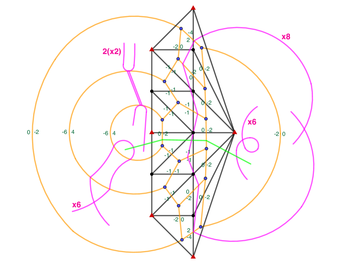
Figure 6. A divisor model of type $Y_{2}Y_{8}I_{8}X_{6}$.

7C. Moduli of $d$-semistable divisor models

In this section we understand the condition of $d$-semistability on our elliptically fibered surfaces $X_{0,LR}(\ell)$. Let $X_{0}$ denote a Kulikov surface, that is, a topologically trivial deformation of the central fiber of a Kulikov model $X\to(C,0)$. For example, $X_{0,LR}(\ell)$ is a Kulikov surface.

Definition 7.16.

We say $X_{0}$ is $d$-semistable if $\mathcal{E}xt^{1}(\Omega^{1}_{X_{0}},\mathcal{O}_{X_{0}})={\mathcal{O}}_{(X_{0})_{\rm sing}}.$

By [Fri83], $X_{0}$ is the central fiber of a Kulikov model if and only if it is $d$-semistable. We recall some basic statements about $d$-semistable Kulikov surfaces from [FS86, Laz08, GHK15b]. Let $X_{0}$ be a Type III Kulikov surface with irreducible components $V_{i}$ and double curves $D_{ij}=V_{i}\cap V_{j}$. One defines the lattice of “numerical Cartier divisors”

$$L=\ker\big{(}\oplus_{i}\operatorname{Pic}V_{i}\to\oplus_{i<j}\operatorname{Pic}D_{ij})$$

with the homomorphism given by restricting line bundles and applying $\pm 1$ signs. The map is surjective over ${\mathbb{Q}}$ by [FS86, Prop. 7.2]. The set of isomorphism classes of not necessarily $d$-semistable Type III Kulikov surfaces of the combinatorial type $X_{0}$ is isogenous to $\operatorname{Hom}(L,{\mathbb{C}}^{*})$.

The period point [FS86, Sec. 3] associated to $X_{0}$ is an element $\psi\in\operatorname{Hom}(L,{\mathbb{C}}^{*})$. It inputs a collection of line bundles $L_{i}\in\operatorname{Pic}V_{i}$ whose degrees agree on double curves $L_{i}\cdot D_{ij}=L_{j}\cdot D_{ji}$ and measures an obstruction in $\mathbb{C}^{*}$ to their gluing together to form a line bundle on $X_{0}$. In particular, the Picard group of the surface $X_{0}$ is $\ker(\psi)$. The surface is $d$-semistable iff the following divisors are Cartier: $\xi_{i}=\sum_{j}D_{ij}-D_{ji}\in L$. Note that $\sum_{i}\xi_{i}=0$. Thus, the $d$-semistable surfaces correspond to the points of multiplicative group $\operatorname{Hom}({\mathbb{L}},{\mathbb{C}}^{*})$, where

$$\Xi=\frac{\oplus_{i}{\mathbb{Z}}\xi_{i}}{(\sum_{i}\xi_{i})},\qquad{\mathbb{L}}=\operatorname{coker}(\Xi\to L).$$

There is a symmetric bilinear form on $L$ defined by $(R_{i})^{2}:=\sum R_{i}^{2}$ which descends to $\mathbb{L}$ because $\Xi$ is null (in fact it generates the null space over $\mathbb{Q}$). Define $\overline{\mathbb{L}}:=\mathbb{L}/(\rm tors)$.

Definition 7.17.

Call a surface $X_{0}$ with $\psi=1\in\operatorname{Hom}(L,\mathbb{C}^{*})$ a standard surface.

Proposition 7.18.

Let $X_{0,LR}(\ell)$ be an elliptically fibered divisor model as in Definition 7.13. The classes of the fibers of the fibration

$$X_{0,LR}(\ell)\to\mathbb{P}^{1}\cup\dots\cup\mathbb{P}^{1}$$

reduce to the same class in $\mathbb{L}$.

Proof.

Let $f_{i}$ be a fiber of the fibration over a non-nodal point on the $i$th $\mathbb{P}^{1}$. Define $\sigma_{i}:=\sum_{j\in S_{i}}\xi_{j}$ where $S_{i}$ denotes the set of components which fiber over a $\mathbb{P}^{1}$ with index less than $i$. Then $[f_{i}]-[f_{1}]=\sigma_{i}$. Hence $[f_{i}]$ and $[f_{1}]$ define the same class in $\mathbb{L}$ for all $i$, which we denote by $f$. ∎

Lemma 7.19.

A standard surface $X_{0,LR}(\ell)$ is elliptically fibered.

Proof.

Consider a vertical chain of rational curves as in Definition 7.10 on $X_{0,LR}(\ell)$, which is not, a priori, elliptically fibered. This vertical chain defines a class $f_{i}\in L$ and it is easy to check that $\psi(f_{i})$ is the element of $\mathbb{C}^{*}$ which makes the two ends of the chain match on the appropriate double curve. Since $\psi(f_{i})=1$, the chain $f_{i}$ closes into a cycle. Since the standard surface is $d$-semistable, Proposition 7.18 implies all vertical strips of $X_{0,LR}(\ell)$ are fibered.

Similarly, there is a unique way to successively glue the components of the section $s$ into a chain from left to right, except possibly that the section at the right end doesn’t match up. The mismatch is an element of $\mathbb{C}^{*}$ equal to $\psi(s)$. Hence $s$ glues to a section on the standard surface. ∎

Proposition 7.20.

The moduli space of $d$-semistable elliptically fibered surfaces $X_{0,LR}(\ell)$ is isogenous to the torus $\operatorname{Hom}(\overline{\mathbb{L}}/\mathbb{Z}f\oplus\mathbb{Z}s,\mathbb{C}^{*})\cong(\mathbb{C}^{*})^{17}$. In particular, all deformations which keep $f$ and $s$ Cartier are elliptically fibered.

Proof.

By Proposition 7.19, a $d$-semistable elliptically fibered surface exists. Given one, the $d$-semistable topologically trivial deformations are locally parameterized by the $19$-dimensional torus $\operatorname{Hom}(\overline{\mathbb{L}},\mathbb{C}^{*}).$ Those that keep $s$ and $f$ Cartier are thus identified with the $17$-dimensional subtorus for which $\psi(f)=\psi(s)=1$. Starting with the elliptically fibered standard surface $X_{0,LR}(\ell)$, the arguments in Lemma 7.19 imply that keeping $s$ and $f$ Cartier preserves the condition of being elliptically fibered. The converse is also true, so the proposition follows. ∎

The space of $d$-semistable deformations of $X_{0,LR}(\ell)$ which keep $f$ and $s$ Cartier is $18$-dimensional and smooth and the $17$-dimensional subspace of topologically trivial deformations is a smooth divisor.

Definition 7.21.

Let $X_{0}$ be any Kulikov model. Define for any component $V_{i}$ the lattice $\widetilde{\Lambda}_{i}:=\{D_{ij}\}^{\perp}\subset H^{2}(V_{i},\mathbb{Z})$. Then there is an inclusion $\iota_{i}\colon\widetilde{\Lambda}_{i}\hookrightarrow L$ sending $\lambda\in\widetilde{\Lambda}_{i}$ to the numerically Cartier divisor which is $\lambda$ on $V_{i}$ and $0$ on all other components. Now suppose that $X_{0}=X_{0,LR}(\ell)$ is elliptically fibered. Define $\Lambda_{i}$ to be the image of $\widetilde{\Lambda}_{i}$ in $\overline{\mathbb{L}}/\mathbb{Z}f\oplus\mathbb{Z}s$ and let $\Lambda:=\oplus\Lambda_{i}$.

Concretely, $\widetilde{\Lambda}_{i}$ is zero unless $Q(V_{i})>0$ and it maps isomorphically to $\Lambda_{i}$ unless $V_{i}$ is an $X$-type end surface, in which case the map to $\Lambda_{i}$ quotients by $\mathbb{Z}f$.

Remark 7.22.

By Proposition 7.20, it is possible to realize any homomorphism $\operatorname{Hom}(\Lambda,\mathbb{C}^{*})$ as the restriction of the period map $\psi$ of some $d$-semistable elliptically fibered surface. Following [GHK15b], [Fri15] the period point of the anticanonical pair $(V_{i},\sum_{j}D_{ij})$ is the restriction homomorphism

$$\psi_{i}\colon\widetilde{\Lambda}_{i}\to{\rm Pic}^{0}(\textstyle\sum_{j}D_{ij})\cong\mathbb{C}^{*}$$

and this period map is compatible with the inclusion of $\widetilde{\Lambda}_{i}$ into $L$ in the sense that $\psi\circ\iota_{i}=\psi_{i}$. Thus, any period point of any component $V_{i}$ can be realized by some $d$-semistable elliptically fibered surface, except for the case when $V_{i}$ is an $X$-type end, where the extra condition $\psi_{i}(f)=1$ ensures either of the equivalent conditions that (1) $\psi_{i}$ descends to $\Lambda_{i}$ or (2) $V_{i}$ is elliptically fibered in class $f$.

7D. Limits of elliptic fibrations

We prove in this section that $X_{0,LR}(\ell)$ is a limit of elliptically fibered K3 surfaces and that the very singular fibers (cf. Definition 7.14) are the limits of the correct number of singular fibers.

Proposition 7.23.

Let $X_{LR}(\ell)\rightarrow C$ be a smoothing of an elliptically fibered $X_{0,LR}(\ell)$ which keeps $f$ and $s$ Cartier. Then the general fiber is an elliptic K3 surface, the very singular fibers are the limits of the singular fibers, and the section $s$ is the limit of the section.

Proof.

Let $f$ be some fiber. Since we keep $s$ and $f$ Cartier, there are line bundles $L_{s}$ and $L_{f}$ on $X_{LR}(\ell)$ which when restricted to the central fiber are $\mathcal{O}(s)$ and $\mathcal{O}(f)$ respectively. By constancy of the Euler characteristic, $\chi(\mathcal{O}(s))=1$ and $\chi(\mathcal{O}(f))=2$. Since $h^{0}({\mathcal{O}}(s))=1$, $h^{0}({\mathcal{O}}(f))=2$ and $h^{0}({\mathcal{O}}(-s))=h^{0}({\mathcal{O}}(-f))=0$ on every fiber, it follows from Serre duality that $h^{1}(\mathcal{O}(s))=h^{1}(\mathcal{O}(f))=0$ on every fiber. By Cohomology and Base Change [Har77, III.12.11] we conclude that $H^{0}(L_{s})$ and $H^{0}(L_{f})$ surject onto the corresponding spaces of sections on the central fiber. Thus, we can ensure that $s$ and $f$ are flat limits of curves. Note that for any choice of $f$, the line bundle $L_{f}$ is the same on the general fiber, and so any $f$ is the limit of a section from the same linear system.

A local analytic model of the smoothing shows that any simple node of a fiber of $X_{0,LR}(\ell)\rightarrow\mathbb{P}^{1}\cup\cdots\cup\mathbb{P}^{1}$ lying on a double curve gets smoothed. So any representative of $f$ which is not very singular is the limit of a smooth genus $1$ curve: Each node lies on the double locus. Similarly, the nodes of $s$ are necessarily smoothed to give a smooth genus $0$ curve. So the general fiber of $X_{LR}(\ell)$ is an elliptic K3 surface with fiber and section classes $f$ and $s$.

Thus, the only fibers which can be limits of singular fibers of the elliptic fibration are the very singular fibers. If the ends are $L,R=1$, the generic choice of $X_{0,LR}(\ell)$ has $24$ distinct very singular fibers with only one node not lying on a double curve. Hence they must be limits of at worst $I_{1}$ Kodaira fibers on a smoothing. By counting, each very singular fiber is the flat limit of an $I_{1}$ fiber.

It remains to show that the when $\ell_{1}>0$ for end type $L$ or $R=2,3$ the two non-reduced vertical components of $R$ are each limits of two singular fibers. This again follows from counting, along with a monodromy argument which shows these two components of $R$ must be limits of an equal number of singular fibers.

Finally when $X_{0,LR}(\ell)$ is not generically chosen, is it a limit of such. This allows us to determine the multiplicities in all cases. ∎

Remark 7.24.

A consequence of Proposition 7.23 is that on any degeneration of elliptic K3 surfaces, the limit of any individual fiber or the section in the divisor or stable model is Cartier (though a priori, only the limit of $s+m\sum f_{i}$ need be Cartier).

7E. The monodromy theorem

We begin with a well-known result on the monodromy of Kulikov/nef models:

Theorem 7.25 ([FS86]).

Let $X\to C$ be a Type II or III degeneration of $\mathbb{M}$-lattice polarized K3 surfaces. Then the logarithm of monodromy on $H^{2}(X_{t})$ of a simple loop enclosing $0\in C$ has the form $\gamma\mapsto(\gamma\cdot\delta)\lambda-(\gamma\cdot\lambda)\delta$ for $\delta$ isotropic, $\delta\cdot\lambda=0$, and $\lambda^{2}=\#\{\textrm{triple points of }X_{0}\}.$ Furthermore $\lambda,\delta\in\mathbb{M}^{\perp}$. There is a homomorphism $\overline{\mathbb{L}}\rightarrow\{\delta,\lambda\}^{\perp}/\delta$ which is an isometry and respects $\mathbb{M}$.

To compute the monodromy invariant $\lambda$ of the degeneration $X_{LR}(\ell)$ requires constructing an explicit basis of the lattice $\delta^{\perp}/\delta$, to coordinatize the cohomology.

Definition 7.26.

Let $B$ be a generic $\operatorname{IAS}^{2}$. A visible surface is a $1$-cycle valued in the integral cotangent sheaf $T^{*}_{\mathbb{Z}}B$. Concretely, it is a collection of paths $\gamma_{i}$ with constant covector fields $\alpha_{i}$ along $\gamma_{i}$ such that at the boundaries of the paths, the vectors $\alpha_{i}$ add to zero in $T^{*}_{\mathbb{Z}}B$. When the paths $\gamma_{i}$ are incident to an $I_{1}$ singularity, the covectors $\alpha_{i}$ must sum to a covector vanishing on the monodromy-invariant direction. Such a visible surface is notated $\gamma=\{(\gamma_{i},\alpha_{i})\}$.

Example 7.27.

The simplest example of a visible surface is a path connecting two $I_{1}$ singularities with parallel monodromy-invariant lines (under parallel transport along the path). Another example is an integral-affine divisor $R_{{\rm IA}}$: It is the special case where the paths are straight lines $e_{ij}$ and the cotangent vector field is $n_{ij}$ times the primitive integral covector vanishing along the corresponding edge.

Following [Sym03], if $B$ is a generic $\operatorname{IAS}^{2}$, there is a symplectic four-manifold $(S,\omega)$ diffeomorphic to a K3 surface, together with $\mu\colon(S,\omega)\rightarrow B$ a Lagrangian torus fibration over $B$ that has $24$ singular fibers over the $I_{1}$ singularities. From a visible surface $\gamma$ one can build from cylinders a surface $\Sigma_{\gamma}\subset S$ fibering over $\gamma$. Its fundamental class is well-defined in $F^{\perp}/F$, where $F=[\mu^{-1}({\rm pt})]$ is the Lagrangian fiber class. Its symplectic area can be computed as

$$[\omega]\cdot[\Sigma_{\gamma}]=\sum_{i}\int_{\gamma_{i}}\alpha_{i}(\gamma_{i}^{\prime}(t))\,dt$$

and so in particular, for any integral-affine divisors $R_{{\rm IA}}$ we have $[\omega]\cdot[\Sigma_{R_{{\rm IA}}}]=0.$ Furthermore, the symmetric bilinear form

$$\gamma\cdot\nu=\{(\gamma_{i},\alpha_{i})\}\cdot\{(\nu_{j},\beta_{j})\}:=\sum_{p\in\gamma\,\cap\,\nu}(\gamma_{i}\cdot\nu_{j})_{p}\det(\alpha_{i},\beta_{j})_{p}$$

agrees with the intersection number $[\Sigma_{\gamma}]\cdot[\Sigma_{\nu}]$ in $F^{\perp}/F$. The relevance of the symplectic geometry lies in the following theorem:

Theorem 7.28 (Monodromy Theorem).

[EF21, Prop.3.14], [AET19, Thm.8.38] Suppose that $B=\Gamma(X_{0})$ is generic and the dual complex of a Type III Kulikov model. There is a symplectic K3 manifold $S$ with a Lagrangian torus fibration over $B$, and a diffeomorphism $\phi\,:S\rightarrow X_{t}$ to a nearby smooth fiber such that

1. $\phi_{*}[F]=\delta$

2. $\phi_{*}[\omega]=\lambda$

Furthermore, if $R$ is an integral-affine divisor, then $R$ determines both an element $[R]\in\mathbb{L}$ and a visible surface $\Sigma_{R}\subset S$. The image of $[R]$ under the map $\overline{\mathbb{L}}\rightarrow\{\delta,\lambda\}^{\perp}/\delta$ from Theorem 7.25 is the same as $\phi_{*}[\Sigma_{R}]$.

By choosing a collection of visible surfaces $\gamma$, we may produce coordinates on the lattice $\delta^{\perp}/\delta$ which allow us to determine how the classes $\lambda$ sit relative to various classes. But, to employ this technique for general $X_{0}$ we must first factor all singularities with charge $Q>1$ into $I_{1}$ singularities, and only then apply the Monodromy Theorem. We describe this process when all $\ell_{i}>0$ but the general case follows from a limit argument.

Consider $B_{LR}(\ell)$. Let $f_{{\rm IA}}$ and $s_{{\rm IA}}$ be the integral-affine divisors corresponding to the fiber $f$ and section $s$ of $X_{0,LR}(\ell)$, respectively. We have described in Table 3 toric models for the $Q=2$ and $Q=3$ singularities. We may flop all the exceptional $(-1)$-curves in these toric models in the smooth threefold $X_{LR}(\ell)$. This has the effect of blowing down these $(-1)$-curves and blowing up the intersection point with the double curve on the adjacent component. In particular, the left and right ends of the section $s$ are $(-1)$-curves which get flopped.

By first making a base change of $X_{LR}(\ell)\rightarrow C$ and resolving to a new Kulikov model, we may ensure that the $(-1)$-curves get flopped onto toric components. This gives a new Kulikov model $X_{0,LR}^{\prime}(\ell)$ with $24$ distinct $I_{1}$ singularities. The effect of these modifications on the dual complex is to first refine the triangulation (the base change), then factor each singularity into $I_{1}$ singularities, moving each one one unit of lattice length in its monodromy-invariant direction (the flops). These $I_{1}$-factorization directions are listed for the various end singularities in Table 3.

Definition 7.29.

We define $19$ visible surfaces $\gamma_{i}\in\{s_{{\rm IA}},f_{{\rm IA}}\}^{\perp}$ in the dual complex $\Gamma(X_{0,LR}^{\prime}(\ell))$ as follows: If $\ell_{i}\vec{v}_{i}$ connects two $I_{1}$ singularities, then $\gamma_{i}$ is the path along the vector $\ell_{i}\vec{v}_{i}$ connecting them as in Example 7.27. For $i=1,2,3$ and all end behaviors, the visible surfaces $\gamma_{i}$ are uniquely defined by the following properties:

1. $\gamma_{i}$ is supported on the edge $\ell_{i}\vec{v}_{i}$ and the segments along which the $I_{1}$-factorization occurs of the singularities at the two ends of $\ell_{i}\vec{v}_{i}$.

2. The support of $\gamma_{1}$ does not contain the $I_{1}$-factorization direction corresponding to the section $s$.

3. $\gamma_{i}$ is integral, primitive, and $[\omega]\cdot\Sigma_{\gamma_{i}}$ is a positive integer multiple of $\ell_{i}$.

Example 7.30.

The visible surface $\gamma_{1}$ has weights $-1,0,1$ along the $I_{1}$ factorization directions $(1,-3),(1,0),(1,3)$ respectively of $X_{3}$ and is balanced by a unique choice of covector along the edge $\ell_{1}\vec{v}_{1}$. Here the “weight” is the multiplicity of the primitive covector vanishing on the monodromy-invariant direction of the $I_{1}$ singularity at the end of the segment. The covector that $\ell_{1}\vec{v}_{1}$ carries ends up being three times the primitive covector vanishing on the monodromy-invariant direction at the endpoint of $\ell_{1}\vec{v}_{1}$.

As we are henceforth concerned only with intersection numbers, we lighten the notation by simply writing $\gamma$ for $\phi_{*}[\Sigma_{\gamma}]$.

Proposition 7.31.

The classes $\lambda=\phi_{*}[\omega]$ and $\gamma_{i}$ lie in $\{s,f\}^{\perp}$ and their intersection matrices for the three end behaviors are:

$L=1$	$\gamma_{1}$	$\gamma_{2}$	$\gamma_{3}$
$\lambda$	$3\ell_{1}$	$\ell_{2}$	$\ell_{3}$
$\gamma_{1}$	$-8$	$3$	$0$
$\gamma_{2}$	$3$	$-2$	$1$
$\gamma_{3}$	$0$	$1$	$-2$

$L=2$	$\gamma_{1}$	$\gamma_{2}$	$\gamma_{3}$
$\lambda$	$2\ell_{1}$	$2\ell_{2}$	$\ell_{3}$
$\gamma_{1}$	$-8$	$2$	$0$
$\gamma_{2}$	$2$	$-4$	$2$
$\gamma_{3}$	$0$	$2$	$-2$

$L=3$	$\gamma_{1}$	$\gamma_{2}$	$\gamma_{3}$
$\lambda$	$\ell_{1}$	$2\ell_{2}$	$\ell_{3}$
$\gamma_{1}$	$-2$	$1$	$0$
$\gamma_{2}$	$1$	$-4$	$2$
$\gamma_{3}$	$0$	$2$	$-2$

We also have $\gamma_{i}\cdot\gamma_{i-1}=1$, $\gamma_{i}^{2}=-2$, $\lambda\cdot\gamma_{i}=\ell_{i}$ for $i\geq 4$ until the right end.

Proof.

Because the weight of the visible surface $\gamma_{1}$ along the edge corresponding to $s_{{\rm IA}}$ is always zero, so we have $\Sigma_{\gamma_{1}}\cdot\Sigma_{s_{{\rm IA}}}=0$. The other $\gamma_{i}$ are also disjoint from $s_{{\rm IA}}$. Furthermore, all $\gamma_{i}$ are disjoint from some fiber $f_{{\rm IA}}$ and hence $\Sigma_{\gamma_{1}}\cdot\Sigma_{f_{{\rm IA}}}=0$. Because $s_{{\rm IA}}$ and $f_{{\rm IA}}$ are integral-affine divisors, we have $[\omega]\cdot\Sigma_{f_{{\rm IA}}}=[\omega]\cdot\Sigma_{s_{{\rm IA}}}=0$. More generally, the formula $\int_{\Sigma_{\gamma}}\omega=\sum\int\alpha_{i}(\gamma_{i}^{\prime}(t))\,dt$ allows us to compute $[\omega]\cdot\Sigma_{\gamma_{i}}$ for all $i$. The other intersection numbers $\Sigma_{\gamma}\cdot\Sigma_{\nu}$ can be computed via the defined intersection form $\gamma\cdot\nu$ on visible surfaces. Applying $\phi_{*}$ to the aforementioned classes preserves their intersection numbers, giving the tables above. ∎

Corollary 7.32.

After an isometry in $\Gamma$, the classes $\gamma_{i}\in\{s,f\}^{\perp}$ are:

$$L=1 \gamma_{1}=-\beta_{L}, \gamma_{i}=\alpha_{i}\textrm{ for }i\geq 2$$

$$L=2 \gamma_{1}=\beta_{L}, \gamma_{2}=-\gamma_{L}, \gamma_{i}=\alpha_{i}\textrm{ for }i\geq 3$$

$$L=3 \gamma_{1}=\alpha_{2}, \gamma_{2}=\gamma_{L}, \gamma_{3}=\alpha_{1}, \gamma_{i}=\alpha_{i}\textrm{ for }i\geq 4.$$

Proof.

This follows directly from Proposition 7.31. When $L=1,3$ the $\gamma_{i}$ span a lattice isomorphic to $I\!I_{1,17}$ and hence their intersection matrix determines them uniquely up to isometry in $\Gamma$. When $L=2$, the lattice spanned by $\gamma_{i}$ is imprimitive but after adding the integral visible surface $\frac{1}{2}(\gamma_{1}+\gamma_{2})$ it becomes all of $I\!I_{1,17}$ and the same logic applies. Note $\frac{1}{2}(\beta_{L}-\gamma_{L})$ is also integral.∎

Corollary 7.33.

The monodromy invariant of $X_{LR}(\ell)$ is the unique lattice point $\lambda\in\sigma_{LR}$ whose coordinates $a_{i}=\alpha_{i}\cdot\lambda$, $b_{L}=\beta_{L}\cdot\lambda$, $c_{L}=\gamma\cdot\lambda$, $b_{R}=\beta_{R}\cdot\lambda$, $c_{R}=\gamma_{R}\cdot\lambda$ (cf. Section 4C) take the values

$L$ End	$\ell_{1}$	$\ell_{2}$	$\ell_{3}$	$\cdots$	$\ell_{i}$	$\cdots$	$\ell_{17}$	$\ell_{18}$	$\ell_{19}$	$R$ End
$1$	$-b_{L}/3$	$a_{2}$	$a_{3}$				$a_{17}$	$a_{18}$	$-b_{R}/3$	$1$
$2$	$b_{L}/2$	$-c_{L}/2$	$a_{3}$	$\cdots$	$a_{i}$	$\cdots$	$a_{17}$	$-c_{R}/2$	$b_{R}/2$	$2$
$3$	$a_{2}$	$c_{L}/2$	$a_{1}$				$a_{19}$	$c_{R}/2$	$a_{18}$	$3$

Proof.

The monodromy invariant $\lambda=\phi_{*}[\omega]$ is uniquely determined by the tabulated values of $\lambda\cdot\gamma_{i}$ in Proposition 7.31. The result follows from Corollary 7.32. ∎

Definition 7.34.

Let $X(\lambda)\to(C,0)$ be a divisor model of a degeneration of elliptic K3 surfaces whose monodromy invariant is $\lambda\in\sigma_{LR}$. That is, $X(\lambda)=X_{LR}(\ell)$ for an appropriate choice of $\ell$ by Proposition 7.23. From Corollary 7.33 such a model exists whenever

$$b_{L}(\lambda) \equiv b_{R}(\lambda)\equiv 0\pmod{6},$$

$$c_{L}(\lambda) \equiv c_{R}(\lambda)\equiv 0\pmod{2}.$$

Let $X_{0}(\lambda)$ be the central fiber and $B(\lambda):=\Gamma(X_{0}(\lambda))$ be the dual complex.

Remark 7.35.

The divisor model $X(\lambda)$ is not combinatorially unique—various choices were made in its construction, such as how to triangulate $B(\lambda)$. But these choices play no role, since the function of $X(\lambda)$ in the paper is to apply Theorem 3.1. It verifies input (div) and serves an example on which input (d-ss) can be checked.

7F. Type II models

We now describe Type II divisor models. These correspond to when the $\operatorname{IAS}^{2}$ on the dual complex degenerates to a segment. It can do so in two ways.

If $\{L,R\}\in\{2,3\}$ and $\ell_{2}=\cdots=\ell_{18}=0$, the sphere degenerates to a vertical segment. Define a Type II Kulikov model, of combinatorial type ${\widetilde{Y}}_{4}{\widetilde{Y}}_{20}$, associated to the Type II ray ${\widetilde{D}}_{16}$ of ${\mathcal{F}}_{\rm rc}$ as follows:

It is a vertical chain of surfaces. The bottom (${\widetilde{Y}}_{4}$) of the chain is $\mathbb{F}_{2}$. It is glued to the next component up along a genus $1$ curve in the anticanonical class $2(s+2f)$ with $s$ the $(-2)$-section. Next, a sequence of elliptic ruled surfaces glued successively along elliptic sections of the ruling, of self-intersections $-8$ and $8$. At the top of the chain (${\widetilde{Y}}_{20}$) is the blow-up $Bl_{16}\mathbb{F}_{2}$ at $16$ points on a genus $1$ curve in the class $2(s+2f)$, glued along the strict transform of the curve.

We now give the structure of a divisor model. On the top of the chain, the divisor $R$ is the sum of the $16$ reducible fibers of the ruling and four doubled fibers tangential to the double curve. On the bottom it is four doubled fibers tangential to the double curve, plus $16$ fibers of the ruling, plus the $(-2)$-section. On the intermediate surfaces, it is the sum of $16$ fibers and $4$ double fibers. The union of fibers of the rulings on all components form the very singular fibers.

If $\{L,R\}\in\{1,2,3\}$ and $\ell_{1}=\cdots=\ell_{9}=\ell_{11}=\cdots\ell_{19}=0$, the sphere degenerates to a horizontal segment. Define a Type II Kulikov model, of combinatorial type ${\widetilde{X}}_{12}{\widetilde{X}}_{12}$, associated to the Type II ray ${\widetilde{E}}_{8}{\widetilde{E}}_{8}$ of ${\mathcal{F}}_{\rm rc}$ as follows:

The left end (${\widetilde{X}}_{12}$) is a rational elliptic surface. It is glued along a smooth elliptic fiber to a chain of surfaces isomorphic to $E\times\mathbb{P}^{1}$ until the right end (${\widetilde{X}}_{12}$) is reached, which also rational elliptic. The divisor model is defined as follows: The section is an exceptional curve at each end, and a section $\{e\}\times\mathbb{P}^{1}$ on the intermediate components. The very singular fibers are the singular fibers of the elliptic fibrations of the left and right ends.

7G. Stable models and their irreducible components

It remains to describe the stable model resulting from the divisor model $X(\lambda)$. We describe here the components which will appear in the stable model, and prove that in Type III their moduli spaces are affine.

Definition 7.36.

The stable type of a cone in ${\mathcal{F}}_{\rm rc}$ is gotten by the following transformations on ADE type: Bold the symbols $A_{n}$, $E_{n}$, $E^{\prime}_{1}$, replace $D_{n}$ by ${\bf C_{n}}$ and $D_{0},D^{\prime}_{0}$ by ${\bf C_{0}}$. Thus the stable type only fails to distinguish between $D_{0}$ and $D^{\prime}_{0}$; both of them have the stable type ${\bf C_{0}}$. The conversions between the three notations of the paper are summarized in Table 5.

Cones of ${\mathcal{F}}_{\rm rc}$	Singularities of $\operatorname{IAS}^{2}$	Stable types
$E_{k}\,(0\leq k\leq 8)$ and $E_{1}^{\prime}$	$X_{k+3}$ and $X_{4}^{\prime}$	${\bf E_{k}}$ and ${\bf E_{1}^{\prime}}$
$D_{k}\,(0\leq k\leq 17)$ and $D_{0}^{\prime}$	$Y_{2}Y_{2+k}$ and $Y_{2}Y_{2}^{\prime}$	${\bf C_{k}}$ and ${\bf C_{0}}$
$A_{k}\,(0\leq k\leq 17)$	$I_{k+1}$	${\bf A_{k}}$
${\widetilde{E}}_{8}{\widetilde{E}}_{8}$ and ${\widetilde{D}}_{16}$	${\widetilde{X}}_{12}{\widetilde{X}}_{12}$ and ${\widetilde{Y}}_{4}{\widetilde{Y}}_{20}$	${\bf{\widetilde{E}}_{8}{\widetilde{E}}_{8}}$ and ${\bf{\widetilde{C}}_{16}}$

Table 5. Conversions between the three notations

Definition 7.37.

For each possible symbol in the stable type, we define an irreducible stable pair $(X,\Delta+\epsilon R)$ as follows:

${\bf E_{n}}\,(n\geq 0)$, ${\bf E_{1}^{\prime}}$: $X$ is the contraction of an elliptically fibered rational surface with an $I_{9-n}$ fiber along all components of fibers not meeting a section $s$. In particular an $A_{8-n}$ is contracted in the $I_{9-n}$ fiber to give the nodal curve $\Delta$. The divisor $R$ is $s$ plus the images of the singular fibers not equal to $\Delta$. There is an induced lattice embedding $A_{8-n}\subset E_{8}$. For $k=1$, the inclusion $A_{7}\subset E_{8}$ can be either primitive (for the surface ${\bf E_{1}}$) or imprimitive (for the surface ${\bf E_{1}^{\prime}}$).

${\bf A_{n}}\,(n\geq 0)$: Let $(X^{\nu},\Delta^{\nu})$ be the toric anticanonical pair $(\mathbb{F}_{0},s_{1}+f_{1}+s_{2}+f_{2})$. Then $X$ is the result of gluing along the two sections $s_{1}$ and $s_{2}$ via the fibration $|f_{1}|$. The boundary $\Delta$ is the sum of two glued fibers $f_{1}$ and $f_{2}$ and $R$ is another section $s$ plus $n+1$ other nodal fibers.

Restricting to either $s_{1}$ or $s_{2}$ gives a weighted stable curve $({\mathbb{P}}^{1},q_{1}+q_{2}+\epsilon\sum p_{i})$ with two boundary points $q_{1},q_{2}$ and $n+1$ other points $p_{i}$. Stable degenerations of ${\bf A_{n}}$ surfaces are in a bijection with degenerations of such curve pairs and are describe by the well known Losev-Manin space ${\overline{L}}_{n+1}$ [LM00]. Thus, the moduli of ${\bf A_{n}}$ surfaces are reduced to the moduli of curves.

${\bf C_{n}}\,(n\geq 0)$: Let $X^{\nu}=(\mathbb{F}_{1},\Delta_{1}+\Delta_{2})$ be an anticanonical pair with $\Delta_{1}^{2}=0$ and $\Delta_{2}^{2}=4$. Then $X$ is the result of gluing $X^{\nu}$ along the bisection $\Delta_{2}$ by the involution switching the intersection points with the fibration of class $\Delta_{1}$. Here $\Delta$ is $\Delta_{1}$ plus the gluing of $\Delta_{2}$ and $R$ is the $(-1)$-section $s$, plus the sum of $k$ nodal glued fibers not equal to $\Delta$, plus twice the fibers tangent to $\Delta_{2}$. These fibers become cuspidal upon gluing.

Restricting to $\Delta_{2}$ gives a weighted stable curve $({\mathbb{P}}^{1},q^{+}+q^{-}+\epsilon\sum_{i=1}^{k}(p_{i}^{+}+p_{i}^{-}))$ together with an involution $\iota$ exchanging $q^{\pm}$ and $p_{i}^{\pm}$. The stable degenerations of such curve pairs are the $C_{n}$ curves of Batyrev-Blume [BB11], and they are in a bijection with stable degenerations of our surface pairs. Thus, as in the ${\bf A_{n}}$ case, the moduli of ${\bf C_{n}}$ surfaces are reduced to the moduli of curves. One should compare this to Lemma 4.9.

${\bf\widetilde{C}_{16}}$: The Hirzebruch surface $\mathbb{F}_{2}$ glued to itself along a smooth genus $1$ bisection of the ruling, in class $2(s+2f)$. The divisor is the section, plus double the fibers tangent to the bisection which get glued to cuspidal curves, plus $16$ nodal fibers. There is no boundary.

${\bf\widetilde{E}_{8}}$: A rational elliptic surface contracted along all components of fibers not meeting a section $s$. The boundary $\Delta$ is an $I_{0}$ fiber, i.e. a smooth elliptic curve and the divisor $R$ is $s$ plus the sum of the singular fibers.

Given a stable type ${\bf S_{1}}\cdots{\bf S_{N}}$ we define a stable surface as follows: For each symbol ${\bf S_{i}}$ take the corresponding irreducible stable pair listed above, and glue the ${\bf S_{i}}$ together along $\Delta$ such that the sections $s$ glue.

Remark 7.38.

The maximal number of irreducible components of a stable pair is $20$, achieved for the ${\mathcal{F}}_{\rm rc}$ cone $E_{0}A_{0}^{18}E_{0}$ or $\operatorname{IAS}^{2}$ combinatorial type $X_{3}I_{1}^{18}X_{3}$, whose stable type is ${\bf E_{0}A_{0}^{18}E_{0}}$.

Warning 7.39.

All of the above stable pairs are Weierstrass fibrations, normal or non-normal. Thus, they have an elliptic involution $\iota$, and their moduli can be analyzed from the perspective of their $\iota$ quotients, in a manner similar to [AT21]. But the ${\bf ACE}$ surfaces defined above for the rc polarizing divisor are different from the $ADE$ surfaces of [AT21]; the latter are adapted to the ramification polarizing divisor.

Recall the definitions of the root lattices $C_{n}$ ($n\geq 1$) and $E_{n}$ ($n=6,7,8$). The $C_{n}$ lattice is the same as the $D_{n}$ lattice: the sublattice of ${\mathbb{Z}}^{n}(-1)$ of vectors with even sum of coordinates. The Weyl group $W(C_{n})$ is the group ${\mathbb{Z}}_{2}^{n}\rtimes S_{n}$ of signed permutations, and $W(D_{n})$ is the index 2 subgroup ${\mathbb{Z}}_{2}^{n-1}\rtimes S_{n}$ of signed permutations with an even number of sign changes.

$E_{n}$ is the lattice $K_{V}^{\perp}\subset\operatorname{Pic}V$ for a smooth del Pezzo surface $V$ of Picard rank $\rho=n+1$. Their Weyl groups are defined to be generated by reflections in the $(-2)$-vectors. For some small $n$ these definitions give root lattices $E_{5}=D_{5}$, $E_{4}=A_{4}$, $E_{3}=A_{2}A_{1}$. For lower $n$ the definitions still make sense but may produce non-root lattices. In addition, for $\rho=2$ there are two del Pezzo surfaces surfaces ${\mathbb{F}}_{1}$ and ${\mathbb{F}}_{0}$, giving $E_{1}$ and $E^{\prime}_{1}$ respectively. We list the lattices and their Weyl groups for these special cases in Table 6.

Table 6. Lattices $E_{1},E^{\prime}_{1},E_{2}$ and their Weyl groups

Symbol	Lattice	Group			Symbol	Lattice	Group
$E_{1}$	$\langle-8\rangle$	$1$			$E_{2}$	$\begin{pmatrix}-2&1\\ 1&-4\end{pmatrix}$	$W(A_{1})$
$E^{\prime}_{1}$	$\langle-2\rangle$	$W(A_{1})$

Definition 7.40.

For a Dynkin type $A_{n},C_{n},E_{n},E^{\prime}_{1}$, we denote by $\Lambda$ the corresponding root lattice, $T=\operatorname{Hom}(\Lambda,{\mathbb{C}}^{*})$ the torus with this character group, and by $W$ the Weyl group.

Theorem 7.41.

The coarse moduli of stable pairs of type ${\bf A_{n}}$, ${\bf C_{n}}$, ${\bf E_{n}}$, ${\bf E_{1}^{\prime}}$ is $T/W$. The moduli space of stable pairs of a fixed stable type ${\bf S_{1}}\cdots{\bf S_{N}}$ is the product of the moduli spaces for the pairs of types ${\bf S_{i}}$, divided by the LR involution if the type is left-right symmetric.

Proof.

The easiest cases are ${\bf A_{n}}$ and ${\bf C_{n}}$ since they are reduced to the curve case. For ${\bf A_{n}}$ the moduli of such choices is simply a choice of $n+1$ fibers not equal to either component of $\Delta$, up to the $\mathbb{C}^{*}$-action on the base. This gives ${\mathbb{C}}^{*}\backslash({\mathbb{C}}^{*})^{n+1}/S_{n+1}=\operatorname{Hom}(A_{n},{\mathbb{C}}^{*})/W(A_{n})$.

For ${\bf C_{n}}$ surfaces the moduli is given by choosing $n$ fibers $y_{1},\dotsc,y_{n}\in{\mathbb{C}}$ not equal to the irreducible fiber $\Delta$ at $\infty$, modulo $S_{n}$ and the involution $(y_{i})\to(-y_{i})$. Using the maps $y_{i}=x_{i}+\frac{1}{x_{i}}$, this is the same as choosing $(x_{1},\dotsc,x_{n})\in\operatorname{Hom}({\mathbb{Z}}^{n},{\mathbb{C}}^{*})/(\pm)=\operatorname{Hom}(C_{n},{\mathbb{C}}^{*})$ modulo $S_{n}\ltimes{\mathbb{Z}}_{2}^{n}=W(C_{n})$.

The minimal resolution of an ${\bf E_{n}}$ or ${\bf E_{1}^{\prime}}$ surface is a rational elliptic surface $Y$ with a section $s$ and anticanonical $I_{9-n}$ fiber $D=D_{1}+\cdots+D_{9-n}$. One has

$$E_{n}=\{D_{1},\dots,D_{9-n}\}^{\perp}/f=\{s,D_{1},\dots,D_{9-n}\}^{\perp}.$$

Contracting $s$ then successively contracting all but one component of $D$, we see that $E_{n}\cong(K_{V})^{\perp}$ on a del Pezzo surface $V$, so this is the same definition of $E_{n}$ as above. The period torus for the anticanonical pairs preserving the elliptic fibration is $\operatorname{Hom}(E_{n},{\mathbb{C}}^{*})$. Deformations of such pairs always preserve the $(-1)$-section $s$.

The period point $\varphi_{Y}\in\operatorname{Hom}(E_{n},\,\mathbb{C}^{*})$ is given by the restriction map on line bundles $E_{n}\to\operatorname{Pic}^{0}(D)=\mathbb{C}^{*}$. In the current setting, the Torelli theorem for anticanonical pairs [GHK15b, Thm.1.8], [Fri15, Thm.8.7] implies that two such surfaces $Y$ with marked section $s$ and fiber $D$ are isomorphic if and only if there is an element of the finite reflection group $W(E_{n})$ relating their period points $\varphi_{Y}$. Thus the moduli space is $\operatorname{Hom}(E_{n},\mathbb{C}^{*})/W(E_{n})$.

For a stable surfaces of type ${\bf S_{1}\cdots S_{N}}$, the gluings of the components are unique up to an isomorphism, since the components form a chain. So the moduli space is the product of the moduli spaces for the irreducible components, modulo the LR involution if the type is symmetric. ∎

Corollary 7.42.

A type III stratum in ${\overline{F}}^{{\rm rc}}$ of a fixed stable type is affine.

Remark 7.43.

For an $\operatorname{IAS}^{2}$ with a $Y_{2}Y_{2+n}$ or $Y_{2}Y_{2+n}^{\prime}$ end as in Table 3 and Notation 7.5, there is an irreducible component $V$ of a divisor model defining singularity $Y_{n+2}$ or $Y^{\prime}_{2+n}$ of the integral-affine structure. For $Y_{n+2}$ (resp. $Y^{\prime}_{2+n}$), one begins with an anticanonical pair $({\mathbb{F}}_{1},\Delta_{1}+\Delta_{2})$ (resp. $({\mathbb{F}}_{0},\Delta_{1}+\Delta_{2})$), $\Delta_{1}^{2}=0$, $\Delta_{2}^{2}=4$ and blows up $n$ points on $\Delta_{2}$ plus some corner blowups. For $n=0$ these two deformation types are distinct; but once $n>0$ they coincide (which is why we do not require the notation $Y_{2+n}^{\prime}$ for $n>0$).

For $n>0$, the orthogonal complement $\{\Delta_{1},\Delta_{2}\}^{\perp}\subset\operatorname{Pic}V$ to the boundary is the $D_{n}$-lattice, and the group of admissible monodromies is $W(D_{n})$, so the moduli space of anticanonical pairs is $T(D_{n})/W(D_{n})$. Exchanging a pair of points $p_{1},p_{2}\in\Delta_{2}$ which are blown up to their involution partners $\iota p_{1},\iota p_{2}$ gives an anticanonical pair with the same period modulo $W(D_{n})$ but changing only one point $p$ to $\iota p$ changes the period and the isomorphism type of the surface.

However, on the stable model this information is lost: exchanging any point $p$ to $\iota p$ gives the same fiber. So the moduli space of stable pairs is $T(C_{n})/W(C_{n})$, the quotient of $T(D_{n})/W(D_{n})$ by an involution. For $n=0$ there are two types of anticanonical pairs but only one type of stable pairs, so the map to the stable moduli is again $2:1$.

Remark 7.44.

Since the stable degenerations of the ${\bf A_{n}}$ and ${\bf C_{n}}$ surfaces are compatible with the degenerations of the ${\bf A_{n}}$ and ${\bf C_{n}}$ curves, their the moduli spaces come with compactifications of the form $\overline{T}/W$, where $\overline{T}$ is a toric variety for the Coxeter fan of type $A$, resp. $C$. These are moduli spaces of Losev-Manin curves [LM00] and Batyrev-Blume curves [BB11].

For the moduli of ${\bf E_{n}}$ surfaces, taking the star of the corresponding cone in ${\mathcal{F}}_{\rm rc}$ and the closure of $T/W$ in ${\overline{F}}^{\rm rc}$ provides a stable slc pair compactification ${\overline{T}}/W$, where ${\overline{T}}$ is a toric variety for the fan obtained from the $E_{n}$ Coxeter fan by subdiving a Weyl chamber by the hyperplanes $\beta^{\perp}$, $\gamma^{\perp}$ as in Fig. 2. This is a very interesting fan indeed which we investigate further in a forthcoming paper.

Notation 7.45.

We now study the moduli stack of pairs of type ${\bf S}$. To do so, we introduce the following notations: Let $G$ be a discrete group acting properly discontinuously on an analytic space $X$. We notate the coarse space of the quotient by $X/G$ and we notate the stack (orbifold) quotient by $[X:G]$.

For our purposes, we require a more refined notion. Suppose we are given a reflection subgroup $W\subset G$ corresponding to a root system $R$ and for every root $\alpha\in R$ a divisor $\Delta(\alpha)\subset X$ contained in the fixed locus of the reflection $s_{\alpha}$. For any $x\in X$ consider the set of roots $R_{x}=\{\alpha\mid x\in\Delta(\alpha)\}$ and the subgroup $W(R_{x})\subset G_{x}$ in the stabilizer of $x$ generated by the reflections $s_{\alpha}$ with $\alpha\in R_{x}$. Assume that $W(R_{x})$ is a normal subgroup of $G_{x}$ for all $x$. Under these conditions, we define $[X:_{R}G]$ as follows.

For each point $x\in X$, there is an open $G_{x}$-invariant neighborhood $U_{x}\ni x$ where the $G_{x}$-action is approximated by the linear action of $G_{x}$ on the tangent space ${\mathbb{T}}_{x}$, and which satisfies following condition: for any $y\in U_{x}$ one has $G_{y}\subset G_{x}$, $R_{y}\subset R_{x}$, and $W(R_{x})\cap G_{y}=W(R_{y})$. This neighborhood is obtained by applying Luna’s slice theorem and by successfully removing the closed subsets where the above conditions fail. Now define

$$[U_{x}:_{R}G]=[U_{x}/W(R_{x}):G_{x}/W(R_{x})].$$

In words: we take the coarse quotient by $W(R_{x})$ first, and then the stack quotient by the remaining group $G_{x}/W(R_{x})$.

At this point, we recall the theorem of Chevalley, Shephard and Todd [Che55, ST54]: if $G$ is a finite group acting linearly on a complex vector space then $V/G$ is smooth iff $G$ is generated by pseudoreflections, i.e. linear transformations fixing a hyperplane pointwise. For a Weyl group $W$ pseudoreflections are reflections $s_{\alpha}$. In particular, if $U_{x}$ is smooth then so is $U_{x}/W(R_{x})$.

For any $y\in U_{x}$ we can choose an open neighborhood $U_{y}\ni y$ in the same way as above. Since $W(R_{x})\cap G_{y}=W(R_{y})$, the map $U_{y}/W(R_{y})\to U_{x}/W(R_{x})$ is unramified. Thus, the map $[U_{y}:_{R}G]\to[U_{x}:_{R}G]$ is an open embedding, and the stacks $[U_{x}:_{R}G]$ patch together to define the stack $[X:_{R}G]$.

The coarse moduli space of $[X:_{R}G]$ is $X/G$, same as for $[X:G]$, but the stack structure is different: the local reflection groups $W(R_{x})$ are not part of the inertia.

The reason for introducing this notation is that it concisely describes the types of moduli stacks which occur in the presence of a Torelli type theorem, for a more detailed discussion, see [AE21, Rem. 2.36, Thm. 8.12]. For instance, the moduli stack of lattice-polarized ADE K3 surfaces is $[{D}:_{R}G]$ where ${D}$ is the period domain, $G$ is the appropriate arithmetic subgroup of $O(2,19)$, and the root system $R$ consists of the vectors $\alpha$ with $\alpha^{2}=-2$.

We also prove the following Lemma. Using the notations of [Bou02], let $R$ be a root system with a root lattice $Q$, weight lattice $P$ and Weyl group $W$. Denote by $\mu_{R}$ the finite abelian group $\operatorname{Hom}(P/Q,{\mathbb{C}}^{*})$. Then one has the following commutative diagram

(7.1)

It is a basic result of the invariant theory of multiplicative type that one has $\operatorname{Hom}(P,{\mathbb{C}}^{*})/W={\mathbb{A}}^{n}$, with the coordinates on ${\mathbb{A}}^{n}$ equal to the characters of the fundamental weights, see e.g. [Bou05, Ch.8, §7, Thm.2].

For each root $\alpha\in Q$, let $\Delta_{Q}(\alpha)$ be the kernel of the homomorphism $\operatorname{Hom}(Q,{\mathbb{C}}^{*})\to\operatorname{Hom}({\mathbb{Z}}\alpha,{\mathbb{C}}^{*})={\mathbb{C}}^{*}$. Let $\Delta_{P}(\alpha)$ be its preimage in $\operatorname{Hom}(P,{\mathbb{C}}^{*})$. We use these divisors $\Delta_{Q}(\alpha)$, $\Delta_{P}(\alpha)$ to define the $:_{R}$ quotients as in Notation 7.45.

Lemma 7.46.

One has $[\operatorname{Hom}(Q,{\mathbb{C}}^{*}):_{R}W]=[\operatorname{Hom}(P,{\mathbb{C}}^{*})/W:\mu_{R}]=[{\mathbb{A}}^{n}:\mu_{R}]$.

Proof.

The ramification divisor of $\operatorname{Hom}(P,{\mathbb{C}}^{*})\to{\mathbb{A}}^{n}$ is $\cup_{\alpha\in R}\Delta_{P}(\alpha)$, see e.g. [Ste65, 6.4, 6.8]. An easy direct computation shows that the fixed locus of the reflection $s_{\alpha}$ on the weight lattice torus $\operatorname{Hom}(P,{\mathbb{C}}^{*})$ is $\Delta_{P}(\alpha)$.

For $x\in\operatorname{Hom}(P,{\mathbb{C}}^{*})$, let ${\mathbb{T}}_{x}$ be the tangent space at $x$. Since the quotient $\operatorname{Hom}(P,{\mathbb{C}}^{*})/W={\mathbb{A}}^{n}$ is smooth, the quotient ${\mathbb{T}}_{x}/W_{x}$ is smooth as well (this follows from a baby version of Luna’s slice theorem). By the theorem of Chevalley, Shephard and Todd, ${\mathbb{T}}_{x}/W_{x}$ is smooth if and only if $W_{x}$ is generated by pseudo-reflections. Alternatively, we can cite [Bou02], Exercise 7 to Ch.V §5. Pseudoreflections in $W$ are reflections. So $W_{x}$ is generated by the reflections that it contains. (We thank Michel Brion for this argument.)

Now it follows that $[\operatorname{Hom}(P,{\mathbb{C}}^{*}):_{R}W]=\operatorname{Hom}(P,{\mathbb{C}}^{*})/W={\mathbb{A}}^{n}$ and that

$$[\operatorname{Hom}(Q,{\mathbb{C}}^{*}):_{R}W]=[\operatorname{Hom}(P,{\mathbb{C}}^{*}):_{R}(W\times\mu_{R})]=[{\mathbb{A}}^{n}:\mu_{R}].$$

∎

Remark 7.47.

For the action of $W$ on the root lattice torus $\operatorname{Hom}(Q,{\mathbb{C}}^{*})$ it is in general not true that the stabilizer $W_{x}$ coincides with $W(R_{x})$ for all $x$. For example, for $R=A_{2}$ and $W=S_{3}$ there are two points with stabilizer $W_{x}={\mathbb{Z}}_{3}$ and trivial $W(R_{x})$. Also, an explicit computation shows that the fixed locus of a reflection $s_{\alpha}$ on $\operatorname{Hom}(Q,{\mathbb{C}}^{*})$ is $\Delta_{Q}(\alpha)$ if and only if $\alpha$ is primitive in the weight lattice $P$. This holds for all irreducible root $ADE$ lattices except for $A_{1}$, in which case $\Delta_{Q}(\alpha)$ is a single point $\{1\}$ while the fixed locus of the involution $z\to z^{-1}$ is $\{\pm 1\}$.

For a simply laced $ADE$ root system one has $Q=\operatorname{Hom}(P,{\mathbb{Z}})$. For the $C_{n}$ root system one has $P(C_{n})={\mathbb{Z}}^{n}$ and $Q(C_{n})$ the sublattice of vectors with even sums, so that $P/Q={\mathbb{Z}}_{2}$. To simplify notation, we frequently denote the root lattice by the same symbol as the root system, and write $A_{n}$ etc. instead of $Q(A_{n})$ etc.

Theorem 7.48.

The moduli stack of irreducible pairs of type ${\bf S}$ is a $\mu_{2}$-gerbe over:

${\bf S}$	Stack	Group action
${\bf A_{n}}$, $n\geq 0$	$[{\mathbb{A}}^{n}:\mu_{n+1}]$	acting as $\mu_{R}$: $(c_{i})\to(\xi^{i}c_{i})$, $\xi^{n+1}=1$
${\bf C_{n}}$, $n\geq 0$	$[{\mathbb{A}}^{n}:\mu_{2}]$	$(c_{i})\to(-c_{i})$
${\bf E_{n}}$, $n\geq 3$	$[{\mathbb{A}}^{n}:\mu_{9-n}]$	acting as $\mu_{R}=\operatorname{Hom}(P/Q,{\mathbb{G}}_{m})$
${\bf E_{2}}$	${\mathbb{G}}_{m}\times{\mathbb{A}}^{1}$
${\bf E_{1}}$	${\mathbb{G}}_{m}$
${\bf E^{\prime}_{1}}$	$[{\mathbb{A}}^{1}:\mu_{4}]$	for $\mu_{4}=\langle g\rangle$, $g(c)=-c$
${\bf E_{0}}$	$[{\rm pt}:\mu_{3}]$

Here, for the ${\bf A_{n}}$ pairs we fix the left-right orientation.

Proof.

For ${\bf A_{n}},{\bf C_{n}}$ and for ${\bf E_{n}}$ with $n\geq 3$ the result is the direct application of Lemma 7.46. For smaller ${\bf E_{n}}$ we use the explicit normal forms of the surfaces.

For ${\bf A_{n}}$, $\operatorname{Hom}(P,{\mathbb{C}}^{*})$ is the same as the choice of $n+1$ points $p_{i}\in{\mathbb{C}}^{*}$ with $\prod p_{i}=1$, with a choice of the origin, and $\operatorname{Hom}(P,{\mathbb{C}}^{*})/W={\mathbb{A}}^{n}$ is the set of coefficients $(c_{i})$ in the equation $\prod(x+p_{i})=1+c_{1}x+\dotsc+c_{n}x^{n}+x^{n+1}$ which are well defined up to rescaling to $(c_{i})\to(\xi^{i}c_{i})$.

The data for the surface ${\bf C_{n}}$, $\operatorname{Hom}(P,{\mathbb{C}}^{*})=({\mathbb{C}}^{*})^{n}$ is the data for the $n$ points $p_{i}^{+}$ on the bisection $B_{2}\setminus\{0,\infty\}$. These points are well defined up to switching $p_{i}^{+}\to p_{i}^{-}=\iota p_{i}^{+}$ and switching $p_{i}^{+}\to p_{j}^{\pm}$ for $i\neq j$. The quotient is ${\mathbb{A}}^{n}$ with the coefficients $(c_{i})$ giving the equation $x^{n}+c_{1}x^{n-1}+\dotsb+c_{n}$ of the fibers on ${\mathbb{P}}^{1}\setminus\{0,\infty\}/\iota={\mathbb{P}}^{1}\setminus\infty$.

Alternatively, $\operatorname{Hom}(Q,{\mathbb{C}}^{*})$ is the choice of $n$ points $p_{i}^{+}\in{\mathbb{C}}^{*}$ defined up to $p\mapsto-p$, and the moduli stack is $[\operatorname{Hom}(Q,{\mathbb{C}}^{*}):_{R}W]$, giving the same result by Lemma 7.46.

The normal forms for ${\bf E_{6}}$, ${\bf E_{7}}$, ${\bf E_{8}}$ were given in [AT21]. Here, we extend them to ${\bf E_{n}}$ with $0\leq k\leq 5$ and ${\bf E^{\prime}_{1}}$. The quotient by the elliptic involution is $X/\mu_{2}={\mathbb{F}}_{2}$, the double cover is branched in the $(-2)$-section and a trisection. After contracting the $(-2)$-section we get ${\mathbb{P}}(1,1,2)$ and the equation of the trisection is a polynomial $f(x,y)$ of degree 6, where $\deg x=1$ and $\deg y=2$ so that $f(x,y)$ is a cubic in $y$. In affine coordinates $X$ has the equation $z^{2}+f(x,y)=0$.

For a Weierstrass surface $V\to{\mathbb{P}}^{1}$, its minimal resolution ${\widetilde{V}}$ has an $I_{n}$ Kodaira fiber with $n\geq 1$ over $x_{0}\in{\mathbb{P}}^{1}$ iff the equation $f(x_{0},y)$ has a double and a single roots in $y$, see e.g. [Mir89, IV.2.2]. Putting the double root at $y=0$ and the single root at $y=\frac{1}{4}$, we can assume that $f(x_{0},y)=y^{3}-y^{2}/4$. If the nodal fiber is at $x_{0}=\infty$, this means that the degree 6 part of $f(x,y)$ is $y^{3}-(xy)^{2}/4$. By making substitutions $x\to x+a$ and $y\to y+bx+c$ and completing the square, $f(x,y)$ can be put in the following form, unique up to rescaling $x,y$ (cf. [AT21, Sec. 5]):

$$f=y^{3}+c^{\prime}_{2}y^{2}+c^{\prime}_{1}y-\tfrac{1}{4}(xy-c^{\prime\prime})^{2}+c_{0}+c_{1}x+c_{2}x^{2}+c_{3}x^{3}+c_{4}x^{4}+c_{5}x^{5}.$$

This surface has an $I_{n}$ fiber iff its discriminant satisfies $\operatorname{mult}_{x_{0}}\Delta(x)=n$. For $x_{0}=\infty$ this means that $\deg\Delta(x)=12-n$. Putting $f(x,y)$ in the Weierstrass form and computing the normalized discriminant $\Delta_{n}(x)=-2^{4}(4A^{3}+27B^{2})$, we find the following. One has $\deg\Delta_{n}(x)\leq 11$ and the coefficient of $x^{11}$ in $\Delta_{n}$ is $c_{5}$. Thus, the surface $V$ is of type ${\bf E_{8}}$, (i.e. with $I_{1}$ fiber at $x_{0}=\infty$) iff $c_{5}\neq 0$, in which case we can set $c_{5}=1$. If $c_{5}=0$ then $\operatorname{coeff}(x^{10},\Delta_{n})=c_{4}$. Thus $V$ has type ${\bf E_{7}}$ (i.e. with $I_{2}$ fiber at $x_{0}=\infty$) iff $c_{5}=0$ and $c_{4}\neq 0$, and we can set $c_{4}=1$. This argument continues for ${\bf E_{6}},\dotsc,{\bf E_{3}}$.

For ${\bf E_{2}}$, one must have $c_{5}=\dotsb=c_{0}=0$ and then $\operatorname{coeff}({x^{5}},\Delta_{n})=c_{1}^{\prime}c^{\prime\prime}$. We can normalize by setting $c^{\prime\prime}=1$ and take any $c_{1}^{\prime}\neq 0$.

For $k=1$ one must have $c_{1}^{\prime}c^{\prime\prime}=0$. Choosing $c^{\prime}_{1}=0$ gives $\operatorname{coeff}(x^{4},\Delta_{n})=c_{2}^{\prime}(c^{\prime\prime})^{2}$. We normalize by setting $c^{\prime\prime}=1$ and $c^{\prime}_{1}\neq 0$ and call this ${\bf E_{1}}$. Choosing $c^{\prime\prime}=0$ gives $\operatorname{coeff}(x^{4},\Delta_{n})=(c_{1}^{\prime})^{2}$. Normalizing $c^{\prime}_{1}=1$ gives ${\bf E^{\prime}_{1}}$.

Finally, for $k=0$ one must have $c_{1}^{\prime}=c_{2}^{\prime}=0$, and then we normalize $c^{\prime\prime}=1$. We call this case ${\bf E_{0}}$. When $c_{1}^{\prime}=c^{\prime\prime}=0$, one has $\Delta_{n}(x)\equiv 0$, so all fibers are singular. This is a nonnormal surface of type ${\bf C_{0}}$; one may call the fiber at infinity $I_{\infty}$.

Table 7. Normal forms of rational elliptic surfaces with $I_{n}$ fiber

${\bf S}$	$I_{n}$	$c^{\prime}_{2}$	$c^{\prime}_{1}$	$c^{\prime\prime}$	$c_{0}$	$c_{1}$	$c_{2}$	$c_{3}$	$c_{4}$	$c_{5}$	$x^{n}y^{m}$	$G$
${\bf E_{8}}$	$I_{1}$	$\star$	$\star$	$\star$	$\star$	$\star$	$\star$	$\star$	$\star$	$1$	$x^{5}$	$\mu_{1}$
${\bf E_{7}}$	$I_{2}$	$\star$	$\star$	$\star$	$\star$	$\star$	$\star$	$\star$	$1$		$x^{4}$	$\mu_{2}$
${\bf E_{6}}$	$I_{3}$	$\star$	$\star$	$\star$	$\star$	$\star$	$\star$	$1$			$x^{3}$	$\mu_{3}$
${\bf E_{5}}$	$I_{4}$	$\star$	$\star$	$\star$	$\star$	$\star$	$1$				$x^{2}$	$\mu_{4}$
${\bf E_{4}}$	$I_{5}$	$\star$	$\star$	$\star$	$\star$	$1$					$x$	$\mu_{5}$
${\bf E_{3}}$	$I_{6}$	$\star$	$\star$	$\star$	$1$						$1$	$\mu_{6}$
${\bf E_{2}}$	$I_{7}$	$\star$	$\neq 0$	$1$							$xy$	$\mu_{3}$
${\bf E_{1}}$	$I_{8}$	$\neq 0$		$1$							$xy$	$\mu_{3}$
${\bf E^{\prime}_{1}}$	$I_{8}$	$\star$	$1$								$y$	$\mu_{4}$
${\bf E_{0}}$	$I_{9}$			$1$							$xy$	$\mu_{3}$
${\bf C_{0}}$	$I_{\infty}$	$1$									$y^{2}$	$\mu_{2}$

We summarize the results in Table 7 and Fig. 7. The star means the coefficient is arbitrary and we don’t write zeros. The normal forms of this table are unique up to the subgroup $G$ of $({\mathbb{C}}^{*})^{2}$ acting on $x,y$ for which $y^{3}+x^{2}y^{2}+x^{n}y^{m}$ is semi-invariant. The monomial $x^{n}y^{m}$ and the group $G$ are given the last two columns. Taking the quotient of ${\mathbb{A}}^{n}$, resp. of ${\mathbb{G}}_{m}\times{\mathbb{A}}^{k-1}$ by $G$ gives the stacks in the statement of the theorem. For ${\bf E_{2}}$ and ${\bf E_{1}}$, when a ${\mathbb{G}}_{m}$ summand is present, the $\mu_{3}$-action is free.

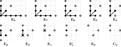
Figure 7. Normal forms of rational elliptic surfaces with $I_{n}$ fiber

∎

For the Type II strata in ${\overline{F}}^{{\rm rc}}$ we have the following:

Theorem 7.49.

For the irreducible pairs the moduli stack of ${\mathbb{Z}}_{2}$-quotients of the stable pairs by the elliptic involution are

$${\bf{\widetilde{E}}_{8}}:\ [\operatorname{Hom}(E_{8},{\mathcal{E}}):_{R}W(E_{8})],\qquad{\bf{\widetilde{C}}_{16}}:\ [\operatorname{Hom}(C_{16},{\mathcal{E}}):_{R}W(C_{16})],$$

where ${\mathcal{E}}$ is the universal family of elliptic curves over their moduli $j$-stack. For the stable pairs of these types the moduli stack is a ${\mathbb{Z}}_{2}$-gerbe over these.

For the surfaces of type ${\bf{\widetilde{E}}_{8}{\widetilde{E}}_{8}}$ the moduli stack is $[\operatorname{Hom}(E_{8}^{2},{\mathcal{E}}):_{R}W(E_{8}^{2})\rtimes{\mathbb{Z}}_{2}]$.

Proof.

By Torelli theorem for anticanonical pairs [GHK15b, Fri15], for a fixed elliptic curve $E$, the moduli of ${\bf{\widetilde{E}}_{8}}$ surfaces is the $:_{R}$-quotient of $\operatorname{Hom}(D^{\perp}/f,E)$ by the group of admissible monodromies, where $D\sim f$ is the boundary, a smooth elliptic curve. We have an identification $D^{\perp}/f=\{D,s\}^{\perp}=E_{8}$, and the group is $W(E_{8})$. A surface of type ${\bf{\widetilde{E}}_{8}{\widetilde{E}}_{8}}$ is glued from two such surfaces along the boundary $D\simeq E$, so we get the product above. The additional ${\mathbb{Z}}_{2}$ is the left-right symmetry. Varying the elliptic curve, for the stack we get the same formulas with $E$ replaced by the universal elliptic curve over the moduli stack of elliptic curves.

A pair $(X,\epsilon R)$ of type ${\bf{\widetilde{C}}_{16}}$ is ${\mathbb{F}}_{2}$ with a smooth bisection $D\sim 2s+4f$, an elliptic curve $E$, plus 16 fibers. The data of the 16 fibers gives a point $(x_{1},\dotsc,x_{16})\in E^{16}$ but defined only up to a 2-torsion (an element of $E[2]$), permuting the points, and dividing by the elliptic involution. One has the exact sequences

$$0\to C_{16}\to{\mathbb{Z}}^{16}\to{\mathbb{Z}}_{2}\to 0\qquad 0\to E[2]\to E^{16}\to\operatorname{Hom}(C_{16},E)\to 0.$$

Therefore a point $(x_{i})$ mod $E[2]$ is an element of $\operatorname{Hom}(C_{16},E)$, and we take the $:_{R}$-quotient of this space by ${\mathbb{Z}}_{2}^{16}\rtimes S_{16}=W(C_{16})$. Varying the elliptic curve $E$ gives the same formulas with $E$ replaced by the universal family ${\mathcal{E}}$. ∎

Remark 7.50.

The commutative diagram (7.1) holds with ${\mathbb{C}}^{*}$ replaced by an elliptic curve $E$. However, it is no longer true in general that $W_{x}=W(R_{x})$, see e.g. the example in [Loo76, 3.6]. The Chevalley-Shephard-Todd’s theorem implies that one has $W_{x}=W(R_{x})$ for all $x$ iff the quotient $\operatorname{Hom}(P,E)/W$ is smooth. By Looijenga [Loo76], $\operatorname{Hom}(P,E)/W$ is a weighted projective space with the weights equal to the coefficients of highest root, and 1. It is frequently singular, e.g. for $R=D_{n}$ ($n\geq 4$) and $E_{n}$ ($n=6,7,8$). Then the coarse quotient $\operatorname{Hom}(P,E)/W$ is singular but the stack $[\operatorname{Hom}(P,E):_{R}W]$ is smooth since it has an étale cover by the local quotients $U_{x}/W(R_{x})$ as in (7.45), which are smooth. Thus, in this case the weighted projective spaces may be considered as smooth orbifolds instead of as singular varieties.

For $E_{8}$, $\operatorname{Hom}(P,E)/W={\mathbb{P}}(1,2^{2},3^{2},4^{2},5,6)$ and for $C_{n}$ it is ${\mathbb{P}}(1^{2},2^{n-1})$. Thus, the alternative description of the boundary divisors is as a family of stacky weighted projective spaces over the $j$-stack of elliptic curves.

7H. Proof of main theorem

In this section we assemble the inputs necessary to apply Theorem 3.1. First, we must show:

Proposition 7.51.

Let $X(\lambda)\rightarrow(C,0)$ be a divisor model with monodromy invariant $\lambda$. The stable model ${\overline{X}}(\lambda)$ (cf. Definition 7.36) has stable type gotten from the combinatorial type (cf. Notation 7.5) of the cone containing $\lambda$.

Furthermore, it is possible to vary $X(\lambda)\rightarrow(C,0)$ so that any stable surface of the given combinatorial type is realized as the stable model ${\overline{X}}(\lambda)$.

Proof.

The first statement follows from seeing which curves are contracted by the linear system of $L_{n}:=n(s+m\sum f_{i})$ for $n\geq 4$ on $X_{0}(\lambda)$. A curve $Z\subset X_{0}(\lambda)$ is contracted iff $L_{n}\cdot Z=0$. Thus the stable model ${\overline{X}}_{0}(\lambda)$ is the result of: (1) contracting the vertical ruling on all components $V_{i}$ not containing the section, then (2) contracting the components $V_{i}$ containing the section but no marked fibers along the horizontal ruling. The resulting surface ${\overline{X}}_{0}(\lambda)$ has the stable type ${\bf S_{1}\cdots S_{N}}$ associated to the cone containing $\lambda$.

We now prove the second statement. First observe that the lattice $\Lambda$ of Definition 7.21 is exactly given by the direct sum

$$\Lambda=\oplus_{i}\,(A\textrm{ or }D\textrm{ or }E)_{n_{i}}$$

corresponding to the components along the top edge of $P_{LR}(\ell)$, i.e. the summands $\Lambda_{i}$ of $\Lambda$ are in fact the character lattices associated to the corresponding symbol ${\bf S_{i}}$ of the stable type, except for switching ${\bf C}$ with $D$, see Remark 7.43.

By Remark 7.22, there is an elliptically fibered $d$-semistable surface $X_{0}(\lambda)$ with period map $\psi\,:\,\overline{\mathbb{L}}/\mathbb{Z}f\oplus\mathbb{Z}s\to\mathbb{C}^{*}$ realizing any element $\psi\big{|}_{\Lambda}\in\operatorname{Hom}(\Lambda,\mathbb{C}^{*})$ and hence any period point of the corresponding anticanonical pair $(V_{i},\sum_{j}D_{ij})$, subject to the condition that if $V_{i}$ is an $X$-type end, it is elliptically fibered.

The element $\psi\big{|}_{\Lambda}$ determines uniquely the locations of the very singular fibers of $X_{0}(\lambda)$ in exactly the same manner that a point in the torus $\operatorname{Hom}(\Lambda_{i},\mathbb{C}^{*})$ determines the modulus of a stable surface: For the singularity $v_{i}=I_{n+1}$ the relative location of two very singular fibers of $X_{0}(\lambda)$ containing the exceptional curves $E_{1}$ and $E_{2}$ on the component $V_{i}$ is $\psi(E_{1}-E_{2})\in\mathbb{C}^{*}$ and hence $\psi\big{|}_{\Lambda_{i}}\in\operatorname{Hom}(A_{n},\mathbb{C}^{*})$ determines the relative locations of the very singular fibers intersecting $V_{i}$. A similar computation holds for type $Y_{2}Y_{2+k}$ and $Y_{2}Y_{2}^{\prime}$ and $\operatorname{Hom}(D_{n},\mathbb{C}^{*})$. By definition, the period point of an elliptically fibered anticanonical pair of type $X_{k+3}$ lies in $\operatorname{Hom}(E_{n},\mathbb{C}^{*})$. It (inexplicitly) determines the location of the singular fibers.

Finally, by Proposition 7.23, the very singular fibers on $X_{0}(\lambda)$ are the limits of singular fibers of the elliptic fibration on the general fiber. These curves contract to the limits of the singular fibers on the stable model. So the restricted period point $\psi\big{|}_{\Lambda}\in\operatorname{Hom}(\Lambda,\mathbb{C}^{*})$ is compatible with the computation of stable moduli made in Theorem 7.41.∎

Lemma 7.52.

The dimensions of a stratum of ${\overline{F}}^{{\mathcal{F}}_{\rm rc}}$ and the dimension of the corresponding moduli space of stable surfaces of fixed type are equal. For Type III strata, the former is equal to $20-\text{(length of its combinatorial type)}$, and the latter to the sum of its Dynkin indices.

Proof.

The dimension of a stratum of the toroidal compactification is the codimension of the corresponding cone. The dimensions of strata in ${\overline{F}}^{{\rm rc}}$ are computed in Theorem 7.41. For type III cones the codimension of the cone and the dimension of the corresponding stable stratum both equal to the sum of the indices $n_{i}$ in the label $(E_{n_{0}}|E^{\prime}_{1}|D_{n_{0}}|D_{0}^{\prime})A_{n_{1}}\dotsc A_{n_{k}}(E_{n_{k+1}}|E^{\prime}_{1}|D_{n_{k+1}}|D_{0}^{\prime})$, resp. with $D$ replaced by ${\bf C}$ and all letters bolded.

For the Type II cones ${\widetilde{E}}_{8}{\widetilde{E}}_{8}$ and ${\widetilde{D}}_{16}$ the strata in ${\overline{F}}^{{\mathcal{F}}_{\rm rc}}$ are divisors, and the dimensions of their image strata ${\bf{\widetilde{E}}_{8}{\widetilde{E}}_{8}}$, ${\bf{\widetilde{C}}_{16}}$ in ${\overline{F}}^{{\rm rc}}$ are $8+8+1=16+1=17$. ∎

Theorem 7.53.

The normalization of the stable pair compactification ${\overline{F}}^{{\rm rc}}$ is the toroidal compactification ${\overline{F}}^{{\mathcal{F}}_{\rm rc}}$.

Proof.

We apply Theorem 3.1 to the case at hand. Taking the divisor model $X(\lambda)$ of Definition 7.34 gives input (div) for the integer $n=6$. Proposition 7.20 implies input (d-ss). Next, the first part of Proposition 7.51 gives input (fan). By (div) and (d-ss), all strata of stable surfaces are been enumerated. Thus, input (qaff) reduces to Corollary 7.42. We conclude that there is a morphism ${\overline{F}}^{{\mathcal{F}}_{\rm rc}}\to{\overline{F}}^{{\rm rc}}$.

Furthermore, this morphism sends toroidal strata to the strata of the corresponding stable types. Thus, the additional condition (dim) follows from Lemma 7.52 if we can prove that the morphisms on strata surject onto the moduli spaces of stable pairs. This follows from the second part of Proposition 7.51, as the restricted period $\psi\big{|}_{\Lambda}$ encodes the image of $0$ under the period map $(C,0)\to{\overline{F}}^{{\mathcal{F}}_{\rm rc}}$. Corollary 3.2 implies the theorem. ∎

Question 7.54.

Having described the normalization of the stable pair compactifications for $R^{\rm ram}$ and $R^{\rm rc}$ it is natural to ask: Is the normalization of the compactification for $tR^{\rm ram}+(1-t)R^{\rm rc}$ toroidal for all $t\in[0,1]$? At what values of $t$ does the compactification change, and how?

7I. The normalization map

Let ${\bf S_{1}\cdots S_{N}}$ be a Type III stable type. By Thm. 7.41 the stratum in ${\overline{F}}^{{\rm rc}}$ of stable pairs $(X,\epsilon R)$ of this type is

$$(T/W^{ACE})/G_{{\rm LR}}$$

where $\Lambda^{ACE}=\oplus_{i=1}^{n}\Lambda_{i}$ is the sum of the $ACE$ lattices of ${\bf S_{i}}$-type, $T=\operatorname{Hom}(\Lambda,{\mathbb{C}}^{*})$ is the corresponding torus, $W^{ACE}=\oplus W(\Lambda_{i})$ is the Weyl group, and $G_{\rm LR}={\mathbb{Z}}_{2}$ if the type is left-right symmetric and trivial otherwise.

Recall once again that the $C_{n}=D_{n}$ as lattices but $W(C_{n})/W(D_{n})={\mathbb{Z}}_{2}$.

Definition 7.55.

For a stable type ${\bf S_{1}\dots S_{N}}$ we have an embedding of the corresponding $ADE$ lattice $\Lambda\subset\textup{II}_{1,17}$: the lattices $\Lambda_{i}$ are generated by the explicit elements of $\textup{II}_{1,17}$, the roots $\alpha_{i}$ and the vectors $\beta_{L}$, $\beta_{R}$, $\gamma_{L}$, $\gamma_{R}$. The generators of the $E_{1}$ and $D_{1}$ lattices are $\beta$ and $\gamma$ respectively. We denote by $\Lambda^{\rm sat}$ the saturation of $\Lambda$ in $\textup{II}_{1,17}$, and by $T^{\rm sat}=\operatorname{Hom}(\Lambda^{\rm sat},{\mathbb{C}}^{*})$ the corresponding torus.

Theorem 7.56.

For the type III strata in ${\overline{F}}^{{\mathcal{F}}_{\rm rc}}$ and ${\overline{F}}^{{\rm rc}}$ the following holds:

1. The only strata of ${\overline{F}}^{{\mathcal{F}}_{\rm rc}}$ glued by the normalization morphism ${\overline{F}}^{{\mathcal{F}}_{\rm rc}}\to{\overline{F}}^{{\rm rc}}$ are the strata $D_{0}\cdots$, $D^{\prime}_{0}\cdots$ (on either left and right ends) both mapping to the ${\bf C_{0}}\cdots$ stratum of ${\overline{F}}^{{\rm rc}}$.

2. For a cone $\sigma$ of the fan ${\mathcal{F}}_{\rm rc}$ with stable type ${\bf S_{1}\cdots S_{N}}$, the corresponding stratum in ${\overline{F}}^{{\mathcal{F}}_{\rm rc}}$ is $(T^{\rm sat}/W^{ADE})/G^{\mathcal{F}}_{{\rm LR}},$ where $G^{\mathcal{F}}_{\rm LR}={\mathbb{Z}}_{2}$ or $1$ depending on whether the cone $\sigma$ is left-right symmetric or not, i.e. $\sigma$ and $\iota\sigma$ are in the same $W(\textup{II}_{1,17})$-orbit for the involution $\iota$, $O^{+}(\textup{II}_{1,17})/W(\textup{II}_{1,17})=\langle\iota\rangle$.

3. The map of strata

   $$(T^{\rm sat}/W^{ADE})/G^{\mathcal{F}}_{{\rm LR}}\longrightarrow(T/W^{ACE})/G_{{\rm LR}}$$

   is defined by the homomorphism of tori $T^{\rm sat}\to T$, dual to the lattice embedding $\Lambda\to\Lambda^{\rm sat}$ and by the $2:1$ map for each $D_{n}\to{\bf C_{n}}$ type with $n>0$.

Proof.

(1) follows from Def. 7.36.

(2) The stratum in ${\overline{F}}^{{\mathcal{F}}_{\rm rc}}$ is the the torus orbit corresponding to $\sigma$, which is $T^{\rm sat}$ as defined, modulo the stabilizer of $\sigma$ in $O^{+}(\textup{II}_{1,17})$, equal to the stabilizer of $\sigma$ in $W(\textup{II}_{1,17})$ plus the involution $\iota$ if the cone $\sigma$ is symmetric. $\operatorname{Stab}_{W(\textup{II}_{1,17})}(\sigma)$ is the stabilizer of the minimal Coxeter cone containing it.

We observe that for each of the cones with the end behavior $E_{1}$, $E^{\prime}_{1}$, $E_{2}$ the stabilizer is the same as the Weyl group of the lattice for its stable type ${\bf E_{1}}$, ${\bf E_{1}^{\prime}}$, ${\bf E_{2}}$, as given in Table 6. For the cones $E_{0}$, $D_{0}$, $D^{\prime}_{0}$ with stable types ${\bf E_{0}}$, ${\bf C_{0}}$ the stabilizers are trivial. The other cones of ${\mathcal{F}}_{\rm rc}$ are already Coxeter cones and for them the stabilizer is obviously the corresponding Weyl group.

(3) As in the proof of Theorem 3.1, we pick a monodromy invariant $\lambda\in\sigma^{0}$ in the interior of the cone and consider a family of divisor models over the partial toroidal compactification ${\overline{F}}^{\lambda}$ with a boundary divisor $\Delta$. The space ${\overline{F}}^{\lambda}$ is an open subset of the blowup of ${\overline{F}}^{{\mathcal{F}}_{\rm rc}}$ at the stratum corresponding to $\lambda$. In terms of the character groups this gives embeddings $\sigma^{\perp}\to\lambda^{\perp}\to\textup{II}_{1,17}.$

On the other hand, as in Section 7C there is a period map $\Delta\to\operatorname{Hom}({\mathbb{L}},{\mathbb{C}}^{*})$, where $L=\ker\big{(}\oplus_{i}\operatorname{Pic}V_{i}\to\oplus_{i<j}\operatorname{Pic}D_{ij})$ and ${\mathbb{L}}=\operatorname{coker}(\Xi\to L)$. In terms of the character lattices it corresponds to the homomorphism ${\mathbb{L}}\to\lambda^{\perp}.$

As in the proof of Prop. 7.51, the composition of this period map and the projection to the periods of the irreducible components of $(X_{0},R_{0})$ is given by the embedding of the character lattices $\Lambda=\oplus\Lambda_{i}\to{\mathbb{L}}.$ Putting this together, we have homomorphisms

$$\sigma^{\perp}\to\lambda^{\perp}\to\textup{II}_{1,17}\quad\text{and}\quad\Lambda\to{\mathbb{L}}\to\lambda^{\perp}.$$

For a one-parameter degeneration $(X,R)\to(S,0)$ of K3 surfaces the period point of the central fiber $X_{0}$ over $\Delta\subset{\overline{F}}^{\lambda}$ is determined by the limit mixed Hodge structure. By [FS86, Prop. 3.4] the map $\Delta\to\operatorname{Hom}({\mathbb{L}},{\mathbb{C}}^{*})$ is defined by the mixed Hodge structure of $X_{0}$. It follows that the map of strata is given by the map of tori with the character groups $\Lambda\to\sigma^{\perp}\cap\textup{II}_{1,17}$.

By comparing the dimensions of the spaces, it follows that the image of $\Lambda\otimes{\mathbb{R}}$ in $\lambda^{\perp}\subset\textup{II}_{1,17}\otimes{\mathbb{R}}$ is $\sigma^{\perp}$ and so $(\operatorname{im}\Lambda)^{\rm sat}=\sigma^{\perp}\cap\textup{II}_{1,17}=\Lambda^{\rm sat}$. ∎

It remains to find the saturation $\Lambda^{\rm sat}$. This is enough to do for the cones with end behavior 1 and 3, since the strata for the end behaviors 2 and 3 are identified by the map ${\overline{F}}^{{\mathcal{F}}_{\rm rc}}\to{\overline{F}}^{{\rm rc}}$. For these cones, the description is given by the next lemma (with a trivial proof), which we apply to the vectors $-\beta_{L},\alpha_{2},\alpha_{3}\dotsc$, resp. $\alpha_{2},\gamma_{L},\alpha_{1},\dotsc$ that satisfy the linear relations (4.2).

Lemma 7.57.

Suppose that vectors $v_{1},\dotsc,v_{19}$ generate $\textup{II}_{1,17}$ with a single linear relation $\sum_{i=1}^{19}n_{i}v_{i}=0$, $n_{i}\in{\mathbb{Z}}$, $\gcd(n_{1},\dotsc,n_{19})=1$. For a subset $I\subset\{1,\dotsc,19\}$ let $\Lambda=\langle v_{i},\ i\in I\rangle$. Then $\Lambda^{\rm sat}/\Lambda={\mathbb{Z}}/d{\mathbb{Z}}$, where $d=\gcd(n_{j},\ j\not\in I)$. We use the convention that $\gcd(0,\dotsc,0)=1$.

Finally, we give a description of the normalization map for the Type II strata.

Theorem 7.58.

The ${\widetilde{E}}_{8}{\widetilde{E}}_{8}$ stratum of ${\overline{F}}^{{\mathcal{F}}_{\rm rc}}$ maps to the ${\bf{\widetilde{E}}_{8}{\widetilde{E}}_{8}}$ stratum of ${\overline{F}}^{{\rm rc}}$ isomorphically. For ${\widetilde{D}}_{16}\to{\bf{\widetilde{C}}_{16}}$, the map of the strata has degree 8 and it is

$$[\operatorname{Hom}(D_{16}^{+},{\mathcal{E}}):_{R}W(D_{16})]\to[\operatorname{Hom}(C_{16},{\mathcal{E}}):_{R}W(C_{16})]$$

where ${\mathcal{E}}$ is the universal elliptic curve over the $j$-stack and $D_{16}^{+}=\textup{II}_{0,16}$.

Proof.

The $1$-cusps of the Baily-Borel compactification ${\overline{F}}^{\rm BB}$ correspond to the primitive isotropic planes $J\subset\textup{II}_{2,18}$. One has $\textup{II}_{2,18}\simeq J\oplus\Lambda\oplus{\widehat{J}}$ for the unimodular lattice $\Lambda=J^{\perp}/J$, and the respective stratum in ${\overline{F}}^{{\mathcal{F}}_{\rm rc}}$ is (the coarse moduli space of) $[\operatorname{Hom}(\Lambda,{\mathcal{E}}):O(\Lambda)]$, cf. [AMRT75, CD07].

For ${\widetilde{E}}_{8}^{2}$ one has $\Lambda=E_{8}^{2}$ and $O(E_{8}^{2})=W(E_{8}^{2})\rtimes{\mathbb{Z}}_{2}$, so we get the same strata in ${\overline{F}}^{{\mathcal{F}}_{\rm rc}}$ and ${\overline{F}}^{{\rm rc}}$ by Theorem 7.49. For ${\widetilde{D}}_{16}$ one has $\Lambda=D_{16}^{+}=\textup{II}_{0,16}$, a $2:1$ extension of $D_{16}$, and $O(D^{+}_{16})=W(D_{16})$, an index 2 subgroup of $W(C_{16})$. So the map of strata is a composition of quotients by ${\mathcal{E}}[2]$ and ${\mathbb{Z}}_{2}$ and it has degree $4\cdot 2=8$. ∎

References

- [AB17] Kenneth Ascher and Dori Bejleri, Log canonical models of elliptic surfaces, Adv. Math. 320 (2017), 210–243.
- [AB19a] by same author, Compact moduli of elliptic K3 surfaces, Preprint (2019), arXiv:1902.10686.
- [AB19b] by same author, Moduli of fibered surface pairs from twisted stable maps, Math. Ann. 374 (2019), no. 1-2, 1007–1032.
- [ABI17] Kenneth Ascher, Dori Bejleri, and Giovanni Inchiostro, Moduli of weighted stable elliptic surfaces and invariance of log plurigenera, Preprint (2017), arXiv:1702.06107.
- [AE21] Valery Alexeev and Philip Engel, Compact moduli of K3 surfaces, arXiv preprint arXiv:2101.12186 (2021).
- [AET19] Valery Alexeev, Philip Engel, and Alan Thompson, Stable pair compactification of moduli of K3 surfaces of degree 2, arXiv:1903.09742.
- [Ale94] Valery Alexeev, Boundedness and for log surfaces, Internat. J. Math. 5 (1994), no. 6, 779–810.
- [Ale02] by same author, Complete moduli in the presence of semiabelian group action, Ann. of Math. (2) 155 (2002), no. 3, 611–708.
- [AMRT75] A. Ash, D. Mumford, M. Rapoport, and Y. Tai, Smooth compactification of locally symmetric varieties, Math. Sci. Press, Brookline, Mass., 1975, Lie Groups: History, Frontiers and Applications, Vol. IV.
- [AN99] Valery Alexeev and Iku Nakamura, On Mumford’s construction of degenerating abelian varieties, Tohoku Math. J. (2) 51 (1999), no. 3, 399–420.
- [AT21] Valery Alexeev and Alan Thompson, ADE surfaces and their moduli, J. Algebraic Geometry 30 (2021), 331–405, arXiv:1712.07932.
- [BB66] W. L. Baily, Jr. and A. Borel, Compactification of arithmetic quotients of bounded symmetric domains, Ann. of Math. (2) 84 (1966), 442–528.
- [BB11] Victor Batyrev and Mark Blume, On generalisations of Losev-Manin moduli spaces for classical root systems, Pure Appl. Math. Q. 7 (2011), no. 4, Special Issue: In memory of Eckart Viehweg, 1053–1084.
- [BL00] Jim Bryan and Naichung Conan Leung, The enumerative geometry of surfaces and modular forms, J. Amer. Math. Soc. 13 (2000), no. 2, 371–410.
- [Bou02] Nicolas Bourbaki, Lie groups and Lie algebras. Chapters 4–6, Elements of Mathematics (Berlin), Springer-Verlag, Berlin, 2002, Translated from the 1968 French original by Andrew Pressley.
- [Bou05] by same author, Lie groups and Lie algebras. Chapters 7–9, Elements of Mathematics (Berlin), Springer-Verlag, Berlin, 2005, Translated from the 1975 and 1982 French originals by Andrew Pressley.
- [Bru15] Adrian Brunyate, A modular compactification of the space of elliptic K3 surfaces, Ph.D. thesis, University of Georgia, 2015, Available at https://getd.libs.uga.edu/pdfs/brunyate_adrian_201508_phd.pdf.
- [CD07] Adrian Clingher and Charles F. Doran, On surfaces with large complex structure, Adv. Math. 215 (2007), no. 2, 504–539.
- [Che55] Claude Chevalley, Invariants of finite groups generated by reflections, Amer. J. Math. 77 (1955), 778–782.
- [EF18] Philip Engel and Simion Filip, Moduli space of integral-affine structures on the sphere, Unpublished (2018).
- [EF21] Philip Engel and Robert Friedman, Smoothings and rational double point adjacencies for cusp singularities, J. Differential Geom. 118 (2021), no. 1.
- [Eng18] Philip Engel, Looijenga’s conjecture via integral-affine geometry, J. Differential Geom. 109 (2018), no. 3, 467–495.
- [FM83] Robert Friedman and Rick Miranda, Smoothing cusp singularities of small length, Math. Ann. 263 (1983), no. 2, 185–212.
- [Fri83] Robert Friedman, Global smoothings of varieties with normal crossings, Ann. of Math. (2) 118 (1983), no. 1, 75–114.
- [Fri15] by same author, On the geometry of anticanonical pairs, Preprint (2015), arXiv:1502.02560.
- [FS86] Robert Friedman and Francesco Scattone, Type degenerations of surfaces, Invent. Math. 83 (1986), no. 1, 1–39.
- [Fuj18] Osamu Fujino, Semipositivity theorems for moduli problems, Ann. of Math. (2) 187 (2018), no. 3, 639–665.
- [GHK15a] Mark Gross, Paul Hacking, and Sean Keel, Mirror symmetry for log Calabi-Yau surfaces I, Publ. Math. Inst. Hautes Études Sci. 122 (2015), 65–168.
- [GHK15b] by same author, Moduli of surfaces with an anti-canonical cycle, Compos. Math. 151 (2015), no. 2, 265–291.
- [GHKS16] Mark Gross, Paul Hacking, Sean Keel, and Bernd Siebert, Theta functions for K3 surfaces, Preprint (2016).
- [Gro66] A. Grothendieck, Éléments de géométrie algébrique. IV. Étude locale des schémas et des morphismes de schémas. (troisième partie), Inst. Hautes Études Sci. Publ. Math. (1966), no. 28, 256.
- [GS03] Mark Gross and Bernd Siebert, Affine manifolds, log structures, and mirror symmetry, Turkish J. Math. 27 (2003), no. 1, 33–60.
- [Har77] Robin Hartshorne, Algebraic geometry, Springer-Verlag, New York, 1977, Graduate Texts in Mathematics, No. 52.
- [HMX18] Christopher D. Hacon, James McKernan, and Chenyang Xu, Boundedness of moduli of varieties of general type, J. Eur. Math. Soc. (JEMS) 20 (2018), no. 4, 865–901.
- [Inc20] Giovanni Inchiostro, Moduli of Weierstrass fibrations with marked section, Adv. Math. 375 (2020), 107374, 57.
- [Kar00] K. Karu, Minimal models and boundedness of stable varieties, J. Algebraic Geom. 9 (2000), no. 1, 93–109.
- [Kaw07] Masayuki Kawakita, Inversion of adjunction on log canonicity, Invent. Math. 167 (2007), no. 1, 129–133.
- [KM97] S. Keel and S. Mori, Quotients by groupoids, Ann. of Math. (2) 145 (1997), no. 1, 193–213.
- [Kol85] János Kollár, Toward moduli of singular varieties, Compositio Math. 56 (1985), no. 3, 369–398.
- [Kol90] János Kollár, Projectivity of complete moduli, J. Differential Geom. 32 (1990), no. 1, 235–268.
- [Kol08] J. Kollár, Hulls and Husks, arXiv: 0805.0576 (2008).
- [Kol13] János Kollár, Singularities of the minimal model program, Cambridge Tracts in Mathematics, vol. 200, Cambridge University Press, Cambridge, 2013, With a collaboration of Sándor Kovács.
- [KP17] Sándor J. Kovács and Zsolt Patakfalvi, Projectivity of the moduli space of stable log-varieties and subadditivity of log-Kodaira dimension, J. Amer. Math. Soc. 30 (2017), no. 4, 959–1021.
- [KS06] Maxim Kontsevich and Yan Soibelman, Affine structures and non-Archimedean analytic spaces, The unity of mathematics, Progr. Math., vol. 244, Birkhäuser Boston, Boston, MA, 2006, arXiv: math.AG/0406564, pp. 321–385.
- [KSB88] J. Kollár and N. I. Shepherd-Barron, Threefolds and deformations of surface singularities, Invent. Math. 91 (1988), no. 2, 299–338.
- [Kul77] Vik. S. Kulikov, Degenerations of surfaces and Enriques surfaces, Izv. Akad. Nauk SSSR Ser. Mat. 41 (1977), no. 5, 1008–1042, 1199.
- [Laz08] Radu Laza, Triangulations of the sphere and degenerations of K3 surfaces, Preprint (2008), arXiv:0809.0937.
- [Laz16] by same author, The KSBA compactification for the moduli space of degree two pairs, J. Eur. Math. Soc. (JEMS) 18 (2016), no. 2, 225–279.
- [LM00] A. Losev and Y. Manin, New moduli spaces of pointed curves and pencils of flat connections, Michigan Math. J. 48 (2000), 443–472.
- [Loo76] Eduard Looijenga, Root systems and elliptic curves, Inventiones mathematicae 38 (1976), no. 1, 17–32.
- [Mir89] Rick Miranda, The basic theory of elliptic surfaces, Dottorato di Ricerca in Matematica. [Doctorate in Mathematical Research], ETS Editrice, Pisa, 1989.
- [Mum72] David Mumford, An analytic construction of degenerating abelian varieties over complete rings, Compositio Math. 24 (1972), 239–272.
- [Nam76] Yukihiko Namikawa, A new compactification of the Siegel space and degeneration of Abelian varieties. I, Math. Ann. 221 (1976), no. 2, 97–141.
- [Oda20] Yuji Odaka, PL density invariant for type II degenerating K3 surfaces, moduli compactification and hyperkahler metrics, Preprint (2020), arXiv:2010.00416.
- [PP81] Ulf Persson and Henry Pinkham, Degeneration of surfaces with trivial canonical bundle, Ann. of Math. (2) 113 (1981), no. 1, 45–66.
- [PSS71] I. I. Pjateckiĭ-Shapiro and I. R. Shafarevič, Torelli’s theorem for algebraic surfaces of type , Izv. Akad. Nauk SSSR Ser. Mat. 35 (1971), 530–572.
- [SB83] N. I. Shepherd-Barron, Extending polarizations on families of surfaces, The birational geometry of degenerations (Cambridge, Mass., 1981), Progr. Math., vol. 29, Birkhäuser, Boston, Mass., 1983, pp. 135–171.
- [Sch73] Wilfried Schmid, Variation of Hodge structure: the singularities of the period mapping, Invent. Math. 22 (1973), 211–319.
- [ST54] G. C. Shephard and J. A. Todd, Finite unitary reflection groups, Canad. J. Math. 6 (1954), 274–304.
- [Ste65] Robert Steinberg, Regular elements of semisimple algebraic groups, Inst. Hautes Études Sci. Publ. Math. (1965), no. 25, 49–80.
- [Sym03] Margaret Symington, Four dimensions from two in symplectic topology, Topology and geometry of manifolds (Athens, GA, 2001), Proc. Sympos. Pure Math., vol. 71, Amer. Math. Soc., Providence, RI, 2003, pp. 153–208.
- [Vie95] Eckart Viehweg, Quasi-projective moduli for polarized manifolds, Ergebnisse der Mathematik und ihrer Grenzgebiete (3) [Results in Mathematics and Related Areas (3)], vol. 30, Springer-Verlag, Berlin, 1995.
- [Vin75] È. B. Vinberg, Some arithmetical discrete groups in Lobačevskiĭ spaces, Discrete subgroups of Lie groups and applications to moduli (Internat. Colloq., Bombay, 1973), Oxford Univ. Press, Bombay, 1975, pp. 323–348.